Data Dieting in GAN Training

Abstract

We investigate training Generative Adversarial Networks, GANs, with less data. Subsets of the training dataset can express empirical sample diversity while reducing training resource requirements, e.g. time and memory. We ask how much data reduction impacts generator performance and gauge the additive value of generator ensembles. In addition to considering stand-alone GAN training and ensembles of generator models, we also consider reduced data training on an evolutionary GAN training framework named Redux-Lipizzaner. Redux-Lipizzaner makes GAN training more robust and accurate by exploiting overlapping neighborhood based training on a spatial 2D grid. We conduct empirical experiments on Redux-Lipizzaner using the MNIST and CelebA data sets.

1 Introduction

In Generative Adversarial Network(GAN) training pathologies such as mode and discriminator collapse can be overcome by using an evolutionary approach wang2018evolutionary ; toutouh2019 . In particular, an evolutionary GAN training method called Lipizzaner has been used for creating robust and accurate generative models toutouh2019 . We work with Redux-Lipizzaner, a descendant of Lipizzaner. Per Lipizzaner, Redux-Lipizzaner operates on spatially distributed populations of generators and discriminators. It executes an asynchronous competitive coevolutionary algorithm on an abstract 2D spatial grid of cells organized into overlapping Moore neighborhoods. On each cell there is a subpopulation of generators and the other of discriminators, aggregated from the cell and its adjacent neighbors. The neural network models’ parameters are updated with stochastic gradient descent following conventional machine learning. Between training epochs, the sub-populations are reinitialized by requesting copies of best neural network models from the cell’s neighborhood. This implicit asynchronous information exchange relies upon overlapping neighborhoods. In contrast to Lipizzaner, only after the final epoch, in Redux-Lipizzaner, the probability weights for each generator ensemble, consisting of a cell and its neighbors, are optimized using an evolutionary strategy. One model in the ensemble is selected probabilistically, on the basis of the weights, to generate the sample.

While it has been shown that mixtures of GANs perform well arora2017gans , one drawback of relying upon multiple generators is that it can be resource intensive to train them. A simple approach to reduce resource use during training is to use less data. For example, different GANs can be trained on different subsamples of the training data set. The use of less training data reduces the storage requirements, both disk and RAM while depending on the ensemble of generators to limit possible loss in performance from the reduction of training data. In the case of Redux-Lipizzaner there is also the potential benefit of the implicit communication that comes from the training on overlapping neighborhoods and updating the cell with the best generator after a training epoch. This leads to the following research questions:

1. How does the accuracy of generators change in spatially distributed grids when the dataset size is decreased?

2. How do ensembles support training with less data in cases where models are trained independently or on a grid with implicit communication?

The contributions of this chapter are:

• Redux-Lipizzaner, a resource efficient method for evolutionary GAN training,

• a method for optimizing GAN generator ensemble mixture weights via evolutionary strategies

• analysis of the impact of data size on GAN training on the MNIST and CelebA data sets

• analysis of the value of ensembling after GAN training on subsets of the data.

We proceed as follows. Notation for this chapter is in Section 2. In Section 3 we describe related work. The Redux-Lipizzaner is described in Section 4. Empirical experiments are reported in Section 5. Finally conclusions and future work are in Section 6.

2 General GAN training

In this study, we adopt the notation similar to arora2017generalization ; li2017towards . Let $\mathcal{G}=\{G_{g},g\in\mathcal{U}\}$ and $\mathcal{D}=\{D_{d},d\in\mathcal{V}\}$ denote the class of generators and discriminators, where $G_{g}$ and $D_{d}$ are functions parameterized by $g$ and $d$. $\mathcal{U},\mathcal{V}\subseteq\mathbb{R}^{p}$ represent the respective parameters space of the generators and discriminators. Finally, let $G_{*}$ be the target unknown distribution to which we would like to fit our generative model.

Formally, the goal of GAN training is to find parameters $g$ and $d$ in order to optimize the objective function

$$\min_{g\in\mathcal{U}}\max_{d\in\mathcal{V}}\mathcal{L}(g,d)\;,\;\text{where}$$

$$\mathcal{L}(g,d)=\mathrm{e}_{x\sim G_{*}}[\phi(D_{d}(x))]+\mathrm{e}_{x\sim G_{g}}[\phi(1-D_{d}(x))]\;,$$ (1)

and $\phi:[0,1]\to\mathbb{R}$, is a concave measuring function. In practice, we have access to a finite number of training samples $x_{1},\ldots,x_{m}\sim G_{*}$. Therefore, an empirical version $\frac{1}{m}\sum_{i=1}^{m}\phi(D_{d}(x_{i}))$ is used to estimate $\mathrm{e}_{x\sim G_{*}}[\phi(D_{d}(x))]$. The same also holds for $G_{g}$.

3 Related Work

Evolutionary Computing and GANs. Competitive coevolutionary algorithms have adversarial populations (usually two) that simultaneously evolve Hillis1990Coev population solutions against each other. Unlike classic evolutionary algorithms, they employ fitness functions that rate solutions relative to their opponent population. Formally, these algorithms can be described with a minimax formulation Herrmann1999Genetic ; Ash2018Reckless which makes them similar to GANs.

Spatial Coevolutionary Algorithms. Spatial (toroidal) coevolution is an effective means of controlling the mixing of adversarial populations in coevolutionary algorithms. Five cells per neighborhood (one center and four adjacent cells) are common Husbands1994Distributed . With this notion of distributed evolution, each neighborhood can evolve in a different direction and more diverse points in the search space are explored. Additional investigation into the value of spatial coevolution has been conducted by Mitchell2006Coevolutionary ; Williams2005Investigating .

Scaling Evolutionary Computing for Machine Learning. A team from OpenAI salimans2017evolution applied a simplified version of Natural Evolution Strategies (NES) wierstra2008natural with a novel communication strategy to a collection of reinforcement learning (RL) benchmark problems. Due to better parallelization over thousand cores, they achieved much faster training times (wall-clock time) than popular RL techniques. Likewise, a team from Uber AI clune2017uber showed that deep convolutional networks with over $4$ million parameters trained with genetic algorithms can also reach results competitive to those trained with OpenAI’s NES and other RL algorithms. OpenAI ran their experiments on a computing cluster of $80$ machines and $1440$ CPU cores salimans2017evolution , whereas Uber AI employed a range of hundreds to thousands of CPU cores (depending on availability). EC-Star hodjat2014maintenance is another example of a large scale evolutionary computation system. By evaluating population individuals only on a small number of training examples per generation, Morse et al. morse2016simple showed that a simple evolutionary algorithm can optimize neural networks of over $1000$ dimensions as effectively as gradient descent algorithms. FCUBE, see https://flexgp.github.io/FCUBE/ is a cloud-based modeling system that uses genetic programming arnaldo2015bring .

Ensembles - Evolutionary Computation and GANs Evolutionary model ensembling has been explored with the aforementioned FCUBE system. FCUBE factors different data splits to cloud instances that model with symbolic regression. These instances draw subsets of variables and fitness functions and learn weakly. After learning the best models are filtered to eliminate the weakest ones and ensemble fusion is used to unify the prediction.

Bagging applies a weighted average to the outputs of a model set for prediction and assumes that all models use the same input variables. Random forests combine bagging with decision trees that use randomized subsets of the input variables. The ensemble technique of Redux-Lipizzaner has weights that bias probabilistic selection of one model in the ensemble to generate a sample in contrast to these techniques which consider all model outputs and average them. There are alternative methods of combining GANs into ensembles. For example, “self-ensembles” of GANs were introduced by Wang2016EnsemblesOG and are constructed with models based on the same network initialization while training for different numbers of iterations. The same authors introduced also cascade GANs where the part of the training data which is badly modeled by one GAN is redirected to a follow-up GAN. Other examples include boosting such as Grover2017BoostedGM and Tolstikhin2017AdaGANBG who present AdaGAN, which adds a new component into a mixture model at each step by running a GAN algorithm on a reweighted sample. MD-GAN Hardy2018MDGANMG distributes GANs so that they can be trained over datasets that are spread on multiple workers. It proposes a novel learning procedure to fit this distributed setup whereas Lipizzaner uses conventional gradient-based training and a probabilistic mixture model. In K-GANS Ambrogioni2019kGANsEO an ensemble of GANs is trained using semi-discrete optimal transport theory. Quoting the authors, “each generative network models the transportation map between a point mass (Dirac measure) and the restriction of the data distribution on a tile of a Voronoi tessellation that is defined by the location of the point masses. We iteratively train the generative networks and the point masses until convergence.” MGAN Hoang2018MGANTG trains with multiple generators given the specific goal of overcoming mode collapse. They add a classifier to the architecture and use it to specify which generator a sample comes from. Essentially, internal samples are created from multiple generators and then one of them is randomly drawn to provide the sample. With the specific aim to provide complete guaranteed mode coverage, Zhong2019RethinkingGC constructing the generator mixture with a connection to the multiplicative weights update rule.

The next section presents Redux-Lipizzaner: a scalable, distributed framework for coevolutionary GAN training with reduced training data use.

4 Data Reduction in Evolutionary GAN Training

This section describes Redux-Lipizzaner which is a spatially distributed coevolutionary GANs training method in which GANs at each cell are trained by using subsets of the whole training data set. The key output of Redux-Lipizzaner is the best performing ensemble (mixture) of generators. First we describe the spatial topology used to evolutionary train GANs in Section 4.1. Next we present how we subsample the training data in Section 4.2. Then in Section 4.3 we describe how the final generator mixture weights are determined. Finally, we formalize the Redux-Lipizzaner algorithm in Section 4.4.

4.1 Overview of Redux-Lipizzaner

Redux-Lipizzaner is an extension of Lipizzaner and addresses the robust training of GANs by employing an adversarial arms races between two populations, one of generators and one of discriminators. Going forward, we use the term adversarial populations to denote these two populations. Thus, we define a population of generators $\mathbf{g}=\{g_{1},\dots,g_{Z}\}$ and a population of discriminators $\mathbf{d}=\{d_{1},\dots,d_{Z}\}$, where $Z$ is the size of the population. These two populations are trained one against the other. The use of populations are one source of diversity, that has shown to be adequate to deal with some of the GAN’s training pathologies schmiedlechner2018towards .

Redux-Lipizzaner defines a toroidal grid. In each cell, it places a GAN (a pair generator-discriminator), which is named center. Each cell has a neighborhood that forms a subpopulations of models: $\mathbf{g}$ (generators) and $\mathbf{d}$ (discriminators). The size of these subpopulations is denoted by $s$. In this study, Redux-Lipizzaner uses five-cell Moore neighborhood ($s=5$), i.e., the neighborhoods include the cell itself (center) and the cells in the west, north, east, and south.

For the $k$-th neighborhood in the grid, we refer to the generator in its center cell by $\mathbf{g}^{k,1}\subset\mathbf{g}$ and the set of generators in the rest of the neighborhood cells by Redux-Lipizzaner $\mathbf{g}^{k,2},\ldots,\mathbf{g}^{k,s}$, respectively. Furthermore, we denote the union of these sets by $\mathbf{g}^{k}=\cup^{s}_{i=1}\mathbf{g}^{k,i}\subseteq\mathbf{g}$, which represents the $k$th generator neighborhood. Note that given a grid size $m\times m$, there are $m^{2}$ neighborhoods. Fig. 1 illustrates some examples of the overlapping neighborhoods on a $4\times 4$ toroidal grid and how the sub-populations of each cell are built ($G_{1,1}$ and $D_{1,1}$). The use of this grid for training the models addresses the quadratic computational complexity of the basic adversarial competitions based algorithms. Without loss of generality, we consider square grids of $m\times m$ size in this study.

Figure 1: Illustration of overlapping neighborhoods on a toroidal grid. Note how a cell update at N_1,2 can be communicated to N_1,1 and N_1,3 when they gather their neighbors. If N_1,1 is then updated with the updated value from N_1,2 the value has propagated. If the propagation continues one more cell to the left to N_1,0, the value will come into the range of both N_0,0 and N_2,0. Propagation runs laterally and vertically. We also show an example of a cell’s generator and discriminator sub-populations (based on its neighborhood) for N_1,1.

The overlapping neighborhoods define the possible exchange of information among the different cells during the training process due to the selection and replacement operators applied in coevolutionary algorithms.

Redux-Lipizzaner is built on the following basis: selection and replacement, fitness evaluation, and reproduction based on GAN training.

Selection and Replacement Selection promotes high performing solutions when updating a subpopulation. Redux-Lipizzaner applies tournament selection of size $\tau$ to update the center of the cell. First, the subpopulations with the updated copies of the neighbors evaluate all GAN generator-discriminator pairs, then $\tau$ generators and $\tau$ discriminators are randomly picked, and the center of the cell is set as the fittest generator and discriminator from the $\tau$ selected ones (lines from 1 to 6 of Algorithm 2). After all GAN training is completed all models are evaluated again, and the tournament selection is applied to replace the least fit generator and discriminator in the subpopulations with the fittest ones and sets them as the center of the cell (lines from 20 to 27 of Algorithm 2).

Fitness Evaluation The search and optimization in evolutionary algorithms are guided by the evaluation of the fitness, a measure that evaluates how good a solution is at solving the problem. In Redux-Lipizzaner, an adversarial method, the performance of the model depends on the adversary. The performance of a given generator (discriminator) is evaluated in terms of some loss function $M$. Redux-Lipizzaner uses Binary cross entropy (BCE) loss (see Equation 2), where the model’s objective is to minimize the Jensen-Shannon divergence (JSD) between the real ($p$) and fake ($q$) data distributions, i.e., $JSD(p\parallel q)$. In Redux-Lipizzaner, fitness $\mathcal{L}$ of a model ($g_{i}\in\mathbf{g}$ or $d_{j}\in\mathbf{d}$) is its average performance against all its adversaries.

$$M^{BCE} =\frac{1}{2}\mathrm{e}_{x\sim G_{g}}[log(1-D_{d}(x))]$$ (2)

Variation - GAN training Model variation is done via GAN training, which is applied in order to update the parameters of the models. Stochastic Gradient Descent training performs gradient-based updates on the parameters (network weights) the models. Moreover, Gaussian-based updates create new learning rate values $n_{\delta}$.

The center generator (discriminator) is trained against a randomly chosen adversary from the subpopulation of discriminators (generators) (lines 9 and 14 of Algorithm 2, respectively).

4.2 Dataset Sampling in Redux-Lipizzaner

Instead of training each sub-population with the whole training dataset, per Lipizzaner, Redux-Lipizzaner applies random sampling with replacement over the training data to define $m^{2}$ different subsets (partitions) of data that will be used as training dataset for each cell (see Figure 2). Thus, each cell has its own training subset of data.

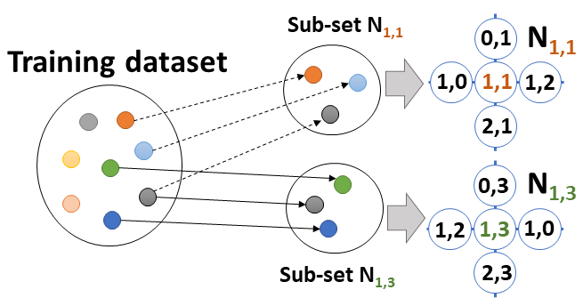
Figure 2: Illustration of how the training dataset is sampled to generate training data subsets to train the different neighborhoods on the grid (N_1,1 and N_1,3).

4.3 Evolving Generator Mixture Weights

Redux-Lipizzaner searches for and returns a mixture of generators composed from a neighborhood. The mixture of generators is the fusion of the different generators in the neighborhood trained by subsets of the training data set. The selection of the best weights that define mixture ensemble is difficult. Redux-Lipizzaner applies an ES-(1+1) algorithm (loshchilov2013surrogate, , Algorithm 2.1) to evolve a mixture weight vector $\mathbf{w}$ for each neighborhood in order to optimize the performance of the fused generative model, see Algorithm 3.

When using Redux-Lipizzaner for images Fréchet Inception Distance (FID) score Martin2017GANs is used to asses the accuracy of the generative models. Note, nothing prevents the use of different metrics, e.g., inception score.

The $s$-dimensional mixture weight vector $\mathbf{w}$ is defined as follows

$$\footnotesize\mathbf{g}^{*},\mathbf{w}^{*}=\operatorname*{argmin}_{\mathbf{g}^{k},\mathbf{w}^{k}:1\leq k\leq m^{2}}\sum_{{g_{i}\in\mathbf{g}^{k}\\ w_{i}\in\mathbf{w}^{k}}}w_{i}FID_{g_{i}},$$ (3)

where $w_{i}$ represents the probability that a data point comes from the $i$th generator in the neighborhood, with $\sum_{w_{i}\in\mathbf{w}^{k}}w_{i}=1$.

4.4 Algorithms of Redux-Lipizzaner

Algorithm 1 formalizes the main steps of Redux-Lipizzaner. First, it starts the parallel execution of the training on each cell by initializing their own learning hyper-parameters (i.e., the learning rate and the mixture weights) and by assigning them their own training subsets (Lines 2 and 3). Then, the training process, see Algorithm 2, consists of a loop with two main steps: first, gather the GANs (neighbors) to build the subpopulations (neighborhood) and, second, update the center by applying the coevolutionary GANs training method for all mini-batches in the training subset. These steps are repeated $T$ (generations or training epochs) times. After that, each cell optimizes its mixture weights by applying an Evolutionary Strategy in order to optimize the performance of the ensemble defined by the neighborhood, see Algorithm 3. Finally, the best performing ensemble is selected across the entire grid and returned, including its probabilistic weights, as the final solution.

Algorithm 1 Redux-Lipizzaner: In parallel, for each cell, initialize settings then iterate over each generation. Each generation, retrieve neighbor cells to build generator and discriminator sub-populations, evolve generators and discriminators trained with SGD, replace worst with best and update self with best, and finally evolve weights for a neighborhood mixture model.
Input:  T : Total generations,  $E$ : Grid cells,  $k$ : Neighborhood size,  $\theta_{D}$ : Training dataset,  $\theta_{p}$ : Sampling size in terms of dataset portion,  $\theta_{COEV}$ : Parameters for CoevolveAndTrainModels,  $\theta_{EA}$: Parameters for MixtureEA
Return:  $n$ : neighborhood,  $\omega$ : mixture weights

1:parfor $c\in E$ do $\triangleright$ Asynchronous parallel execution of all cells in grid

2:    $ds\leftarrow$ getDataSubset($\theta_{D},\theta_{p}$) $\triangleright$ Creates a sub-set of the dataset

3:    $n,\omega\leftarrow$ initializeCells($c,k,ds$) $\triangleright$ Initialization of cells

4:    for generation do $\in[0,\dots,\text{T}]$ $\triangleright$ Iterate over generations

5:         $n\leftarrow$ copyNeighbours($c,k$) $\triangleright$ Collect neighbor cells for the subpopulations

6:         $n\leftarrow$ LipizzanerTraining ($n,\theta_{COEV}$) $\triangleright$ Coevolve GANs using Algorithm 2

7:    end for

8:    $\omega\leftarrow$ MixtureEA($\omega,n,\theta_{EA}$)$\triangleright$ Evolve mixture weights, Algorithm 3

9:end parfor

10:return $(n,\omega)^{*}$ $\triangleright$ Cell with best generator mixture

Algorithm 2 LipizzanerTraining: Select a new neighborhood from the current one. Each mini-batch train discriminators against a randomly drawn generator and generators against a randomly drawn discriminator, using SGD. Evaluate all against each other, using minimum loss as value to choose best to replace worst and update center. Return this new neighborhood.
Input:  $\tau$ : Tournament size,  $X$ : Input training dataset,  $\beta$ : Mutation probability,  $n$ : Cell neighborhood subpopulation,  $ds$ : Sub-set of the training dataset
Return:  $n$ : Cell neighborhood subpopulations

1:$\mathbf{B}\leftarrow$ getMiniBatches($ds$) $\triangleright$ Load mini-batches

2:$B\leftarrow$ getRandomMiniBatch($\mathbf{B}$) $\triangleright$ Get a random mini-batch to evaluate GAN pairs

3:for $g,d\in\mathbf{g}\times\mathbf{d}$ do $\triangleright$ Evaluate all GAN pairs

4:    $\mathcal{L}_{g,d}\leftarrow$ evaluate($g,d,B$) $\triangleright$ Evaluate GAN

5:end for

6:$\mathbf{g},\mathbf{d}\leftarrow$ select($n,\tau$) $\triangleright$ Tournament selection with minimum loss($\mathcal{L}$) as fitness

7:for $B\in\mathbf{B}$ do $\triangleright$ Loop over batches

8:    $n_{\delta}\leftarrow$ mutateLearningRate($n_{\delta},\beta$) $\triangleright$ Update neighborhood learning rate

9:    $d\leftarrow$ getRandomOpponent($\mathbf{d}$) $\triangleright$ Get uniform random discriminator

10:    for $g\in\mathbf{g}$ do $\triangleright$ Evaluate generators and train with SGD

11:         $\nabla_{g}\leftarrow$ computeGradient($g,d$) $\triangleright$ Compute gradient for neighborhood center

12:         $g\leftarrow$ updateNN($g,\nabla_{g},B$) $\triangleright$ Update with gradient

13:    end for

14:    $g\leftarrow$ getRandomOpponent($\mathbf{g}$) $\triangleright$ Get uniform random generator

15:    for $d\in\mathbf{d}$ do $\triangleright$ Evaluate discriminator and train with SGD

16:         $\nabla_{d}\leftarrow$ computeGradient($d,g$) $\triangleright$ Compute gradient for neighborhood center

17:         $d\leftarrow$ updateNN($d,\nabla_{d},B$) $\triangleright$ Update with gradient

18:    end for

19:end for

20:for $g,d\in\mathbf{g}\times\mathbf{d}$ do $\triangleright$ Evaluate all updated GAN pairs

21:    $\mathcal{L}_{g,d}\leftarrow$ evaluate($g,d,B$) $\triangleright$ Evaluate GAN

22:end for

23:$\mathcal{L}_{g}\leftarrow\min(\mathcal{L}_{\cdot,d})$ $\triangleright$ Fitness for generator is the average loss value ($\mathcal{L}$)

24:$\mathcal{L}_{d}\leftarrow\min(\mathcal{L}_{g,\cdot})$ $\triangleright$ Fitness for discriminator is the average loss value ($\mathcal{L}$)

25:$n\leftarrow$ replace($n,\mathbf{g}$) $\triangleright$ Replace the generator with worst loss

26:$n\leftarrow$ replace($n,\mathbf{d}$) $\triangleright$ Replace the discriminator worst loss

27:$n\leftarrow$ setCenterIndividuals($n$) $\triangleright$ Best generator and discriminator are placed in the center

28:return $n$

Algorithm 3 MixtureEA: Evolve mixture weights $\omega$ with a ES-(1+1).
Input:  $GT$ : Total generations to evolve the weights,  $\mu$ : Mutation rate ,  $n$ : Cell neighborhood subpopulation, $\omega$ : Mixture weights
Return:  $\omega$ : mixture weights

1:for generation do $\in[0,\dots,\text{GT}]$ $\triangleright$ Loop over generations

2:    $\omega^{\prime}\leftarrow$ mutate$(\omega,\mu)$ $\triangleright$ Gaussian mutation of mixture weights

3:    $\omega_{f}^{\prime}\leftarrow$ evaluateMixture($\omega^{\prime},n$) $\triangleright$ Evaluate generator mixture score, e.g. FID for images

4:    if $\omega_{f}^{\prime}<\omega_{f}$ then $\triangleright$ Replace if new mixture weights are better

5:         $\omega\leftarrow\omega^{\prime}$ $\triangleright$ Update mixture weights

6:    end if

7:end for

8:return $\omega$

Section 5 next presents results regarding the question of how Redux-Lipizzaner performs given data reduction with the support of ensembles.

5 Experimental Analysis

In this section we proceed experimentally. We use Section 5.1 to present our experimental setup. We then investigate the following research questions:

RQ1:

How robust are spatially distributed grids when training with less of the dataset?

RQ2:

Given the use of ensembles, if we reduce the data quantity at each cell, at what point will the ensemble fail to fuse the resulting models towards achieving sufficient accuracy?

5.1 Experimental Setup

We use two common image datasets from the GAN literature: MNIST lecun1998mnist and CelebA liu2015faceattributes . MNIST has been widely used and it consist of low dimensional handwritten digits images. The larger CelebA dataset contains more than 200,000 images of faces. To obtain an absolute measure of model accuracy, we draw fake image samples from the generative models computed and score them with Frechet inception distance (FID) heusel2017gans . FID score is a black box, discriminator-independent, metric and expresses image similarity to the samples used in training.

The process of sampling the data is independent for each cell of the grid and it consist on randomly selecting different mini-batches of the training dataset. In the context of a grid, given grid size, there is an expectation that every sample will be drawn at least once. This can be considered 100% coverage, over the grid, though not at any cell. When the subset size is lower and/or the grid is smaller, this expected coverage of the complete dataset is nonetheless higher than that of a subset drawn for a single GAN trained independently of others.

For a fixed budget of training samples, when a GAN is trained with a larger dataset and the batch size of a smaller dataset is maintained, the gradient is estimated more often because there are more mini-batches per generation. (Given the standard terminology that an epoch is one forward pass and one backward pass of all the training examples, one epoch is one generation.) In contrast, in the same circumstances, if the number of mini-batches is held constant, and the mini-batch size increased, we incur a cost increase in RAM to store the mini-batch and the gradient is estimated on better information but less frequently. To date, there is no clear well-founded procedure or even a heuristic for setting mini-batch size.

We place all experiments on equal footing by training them with the same budget of mini-batches while keeping mini-batch size, i.e. the number of examples per mini-batch, constant. We experimentally vary the training set size per cell or GAN and adjust the number of generations to arrive at the mini-batch budget. See Equation 4.

$$batches\_to\_train=\frac{training\_dataset\_size}{mini-batch\_size}\times data\_portion\times generations$$ (4)

For example, given a budget of $1.2\times 10^{5}$ mini-batches and a mini-batch size of 100, when the training set size per cell is 60000, there will be 600 mini-batches per generation. We therefore train for 200 generations to reach the $1.2\times 10^{5}$ mini-batches budget. When we reduce the training set size to 30000 ($50\%$), there will be only 300 mini-batches per generation so we train for 400 generations to reach the training budget of $1.2\times 10^{5}$ mini-batches.

Considering the dataset sizes in terms of images (60,000 in MNIST and 202,599 in CelebA), a constant batch size of 100 (Table 2), and the relative training data subset size, we provide the number of generations executed in Table 1. The total number of batches used to train MNIST is 1.20$\times 10^{5}$ and CelebA is 31.66$\times 10^{3}$ when training with the 100% of the data.

Table 1: Batches and generations used in experimental comparisons under equalization to the same computational budget (expressed as batches).

Portion of data	100%	75%	50%	25%
MNIST (Computation budget = 1.20$\times 10^{5}$)
Number of mini-batches	600	450	300	150
Number of generations	200	267	400	800
CelebA (Computation budget = 31.66$\times 10^{3}$)
Number of mini-batches	1583	1187	792	396
Number of generations	20	27	40	80

In this analysis, we compare Redux-Lipizzaner by using different grid sizes (4$\times$4 and 5$\times$5 for MNIST and 3$\times$3 for CelebA) with a Single GAN training method. These different grid sizes allow us to explore the performance of Redux-Lipizzaner according to different degrees of cell overlap. The datasets selected, MNIST and CelebA, represent different challenges for GANs training due to: first, the size of each sample of MNIST (vector of 784 real numbers) is smaller than the same of CelebA (vector of 12,288 real numbers); second, MNIST dataset has fewer number of samples than CelebA, and third, the size of the models (generator-discriminator) are much larger for CelebA generation than for MNIST. This makes the computational resources required to address CelebA higher than for MNIST. Thus, we have defined our experimental analysis taking into account different overlapping patterns and datasets, but also the computational resources available.

All these methods are configured according to the parameterization shown in Table 2. In order to extend our analysis, we apply a bootstrapping procedure to compare the Single GANs with Redux-Lipizzaner. Therefore, we randomly generated 30 populations (grids) of 16 and 25 generators from the 30 generators computed by using Single GAN method. Then, we compute their FIDs and create mixtures to compare these results against Redux-Lipizzaner 4$\times$4 and Redux-Lipizzaner 5$\times$5, respectively. We name these variants Bootstrap 4$\times$4 and Bootstrap 5$\times$5.

Table 2: Setup for experiments conducted with Redux-Lipizzaner on MNIST and CelebA

Parameter	MNIST	CelebA
Coevolutionary settings
Generations	See Table 1
Population size per cell	1	1
Tournament size	2	2
Grid size	1$\times$1, 4$\times$4, and 5$\times$5	3$\times$3
Mixture evolution
Mixture mutation scale	0.01	0.01
Generations	5000	5000
Hyper-parameter mutation
Optimizer	Adam	Adam
Initial learning rate	0.0002	0.00005
Mutation rate	0.0001	0.0001
Mutation probability	0.5	0.5
Network topology
Network type	MLP	DCGAN
Input neurons	64	100
Number of hidden layers	2	4
Neurons per hidden layer	256	$16,384-131,072$
Output neurons	784	$64\times 64\times 3$
Activation function	$tanh$	$tanh$
Training settings
Mini-batch size	100	128

All methods have been implemented in Python3 and pytorch. The experiments are performed on a cloud that provides 16 Intel Cascade Lake cores up to 3.8 GHz with 64 GB RAM and a GPU which are either NVIDIA Tesla P4 GPU with 8 GB RAM or NVIDIA Tesla P100 GPU with 16 GB RAM. All implementations use the same Python libraries and versions to minimize computational differences that could arise from using the cloud.

5.2 Research Question 1: How does the accuracy of generators change in spatially distributed grids when the dataset size is decreased?

We first establish a non-grid baseline by training a single GAN with decreasing amounts of data and examining the resulting FID scores, see Table 3, and Fig. 3 for pairwise statistical significance with a Wilcoxon Rank Sum test with $\alpha=0.01$. What we see is obvious, FID score increases (performance worsens) as the GAN is trained on less data. In 30 runs of single GAN training on $25\%$ of the data, the mean FID score is very high: 574.6 while the standard deviation of FID score is $51.3\%$ including the best FID score of $35.1$. When the data subset is doubled to $50\%$, the mean FID score drops to $71.2$ but the observed standard deviation is higher ($104.6\%$). The best FID score falls to $30.1$. Mean FID score improves with $75\%$ of the data significantly (from $71.2$ to $39.8$) but minimally in terms of the best FID score (30.1 vs 30.2), see Table 4. A marked decrease in standard deviation (104.6% to 12.4%) occurs. In all cases, the smaller training subsets do not match the performance when training with 100% of the data where the best FID score is $27.4$ and the mean FID score is $38.8$, see Table 3 and Table 4. These results are straight forwardly explained by smaller quantities of data failing to sufficiently cover the latent distribution.

Table 3: Mean($\pm$std) of the best FID in the grid for 30 independent runs

Dataset	Variant	25%	50%	75%	100%
MNIST	Single GAN	574.6$\pm$51.3%	71.2$\pm$104.6%	39.8$\pm$12.4%	38.8$\pm$17.0%
MNIST	Single GAN Ensemble	44.2$\pm$9.5%	35.4$\pm$8.0%	34.4$\pm$10.0%	38.6$\pm$12.3%
MNIST	Bootstrap 4$\times$4	578.0$\pm$12.3%	73.5$\pm$25.3%	39.7$\pm$3.0%	38.9$\pm$4.0%
MNIST	Bootstrap 4$\times$4 Ensemble	44.2$\pm$9.0%	35.4$\pm$5.1%	34.5$\pm$6.6%	35.9$\pm$7.4%
MNIST	Redux-Lipizzaner 4$\times$4	47.0$\pm$19.2%	42.0$\pm$16.5%	36.5$\pm$19.2%	37.3$\pm$15.1%
MNIST	Redux-Lipizzaner 4$\times$4 Ensemble	44.1$\pm$21.9%	40.5$\pm$15.4%	33.6$\pm$16.7%	30.7$\pm$17.3%
MNIST	Bootstrap 5$\times$5	573.2$\pm$9.5%	74.8$\pm$22.6%	39.7$\pm$2.3%	38.7$\pm$3.3%
MNIST	Bootstrap 5$\times$5 Ensemble	43.3$\pm$8.3%	33.3$\pm$6.3%	33.0$\pm$5.4%	34.6$\pm$6.7%
MNIST	Redux-Lipizzaner 5$\times$5	39.9$\pm$15.6%	34.4$\pm$9.1%	32.9$\pm$14.2%	34.3$\pm$19.9%
MNIST	Redux-Lipizzaner 5$\times$5 Ensemble	36.2$\pm$16.9%	31.8$\pm$12.6%	30.1$\pm$15.9%	26.3$\pm$16.7%
CelebA	Redux-Lipizzaner 3$\times$3	51.9$\pm$29.8%	50.3$\pm$25.7%	51.3$\pm$26.6%	46.5$\pm$7.3%
CelebA	Redux-Lipizzaner 3$\times$3 Ensemble	49.1$\pm$1.4%	44.7$\pm$6.8%	40.3$\pm$3.9%	43.2$\pm$0.9%

We can now consider competitive coevolutionary grid-trained GANs where there is one GAN per cell, the best of that cell’s training, at the end of execution (see Table 3). This data allows us to isolate the value of the evolutionary training’s communication in contrast to a) the independently trained GANs we previously evaluated and (below) b) the performance impact of ensemble. Recall that the overlapping neighborhoods facilitate signal propagation. GANs which perform well in one neighborhood migrate to their adjacent and overlapping neighborhoods in a form of communication. The grid-trained GANs achieve better FID scores, given the same training budget, than independently trained GANs toutouh2019 . In the case of a 4$\times$4 grid, the experimental mean FID score is 37.3 with a standard deviation of 15.1% and the best generator has a FID score of 26.4. The improvement over independently trained GANs is present with the 5$\times$5 grid, where the experimental mean FID score is 34.3 with a standard deviation of 19.9% and the best generator has a FID score of 20.8. One possible explanation is that the communication indirectly leads to a mixing of the data subsamples (that are drawn independently and with replacement) that effectively improves the coverage of the data.

(a) MNIST 25%

(b) MNIST 50%

(c) MNIST 75%

(d) MNIST 100%

Figure 3: Statistical analysis comparing the same amount of data applying different methods. Black indicates no significance with $\alpha=0.01$

Fig. 3 illustrates the statistical analysis of different methods evaluated here when using the same amount of data. When using the smallest training datasets (MNIST 25%), the use of Redux-Lipizzaner with larger grids and allow significant improvements of the results. The results provided by Redux-Lipizzaner are also improved when the optimization of the mixture weights is applied. With larger datasets (MNIST 75%), Redux-Lipizzaner 4$\times$4 provides results as competitive as the same with 5$\times$5. Something similar is observed when the whole data is used to rain the GANs.

(a) Single GAN

(b) 4$\times$4

(c) 5$\times$5

(d) Single GAN Ensemble

(e) 4$\times$4 Ensemble

(f) 5$\times$5 Ensemble

Figure 4: Statistical analysis comparing the same method with different size of data for MNIST experiments. Black indicates no significance with $\alpha=0.01$. Figures (b), (c), (e), and (f) illustrate the results of Redux-Lipizzaner and their mixtures. Figures (a) and (d) shows the results of bootstrapping and its mixture

Fig. 4 shows illustrates the statistical analysis of the impact on the performance of the methods analyzed here when using different size of training data. Redux-Lipizzaner 4$\times$4 provides similar results when reducing the training data in 25% (i.e., for MNIST 100% and MNIST 75%). When the grid size increases, i.e., Redux-Lipizzaner 5$\times$5, the use o f the training datasets with the half of the data or larger does not show statistical differences in the results. However, the application of the mixtures drives the results with the 100% of the data to be the most competitive ones.

Table 4: Min(best) of the best FID in the grid for 30 independent runs for different data diets

		Data diet
Dataset	Variant	25%	50%	75%	100%
MNIST	Single GAN	35.1	30.1	30.2	27.4
MNIST	Single GAN Ensemble	33.7	30.0	26.9	27.1
MNIST	Bootstrap 4$\times$4	395.5	47.0	37.0	36.1
MNIST	Bootstrap 4$\times$4 Ensemble	33.6	32.7	30.7	28.0
MNIST	Redux-Lipizzaner 4$\times$4	31.8	28.8	27.1	26.4
MNIST	Redux-Lipizzaner 4$\times$4 Ensemble	26.5	28.1	24.6	21.1
MNIST	Bootstrap 5$\times$5	440.8	48.0	37.6	34.9
MNIST	Bootstrap 5$\times$5 Ensemble	34.8	28.1	28.0	29.8
MNIST	Redux-Lipizzaner 5$\times$5	30.5	26.8	27.3	26.3
MNIST	Redux-Lipizzaner 5$\times$5 Ensemble	26.3	21.9	21.2	20.8
CelebA	Redux-Lipizzaner 3$\times$3	39.3	39.0	39.4	42.0
CelebA	Redux-Lipizzaner 3$\times$3 Ensemble	48.3	42.4	38.9	42.7

Scrutinizing Table 3, Fig. 3 and Fig. 4 indicate that Redux-Lipizzaner on a large grid, 5$\times$5, performs among the best for all training data sizes. Furthermore, the Redux-Lipizzaner 4$\times$4 can perform well with reduced training data size. The CelebA results indicate that Redux-Lipizzaner has similar response to data dieting on another data set. Future work on applying Redux-Lipizzaner to address CelebA with larger grid sizes will allow us to confirm this statement. These results lend support to the hypothesis that communication during training can accelerate the impact of small training datasets. We can answer affirmatively, for the datasets we examined, for Redux-Lipizzaner.

5.3 Research Question 2: Given we use ensembles, if we reduce the data quantity at each cell, at what point will the ensemble fail to unify the resulting models towards achieving high accuracy?

We can now consider two directions of inquiry, their order not being important, in the context of the evolutionary GAN training that occurs on a grid. As well, each cell’s neighborhood on the grid defines a sub-population of generators and a sub-population of discriminators which are trained against each other. This naturally suggests the neighborhood to be the set of GANs in each ensemble of the grid, that is, the fusing of each center cell’s generator with its North, South, West and East cell neighbors. We therefore can compare the impact of a neighborhood-based ensemble to each cell’s FID score.

We thus isolate communication from grid-based ensembles and we also isolate co-trained ensembles from ensembles arising from independently trained GANs. For tabular results see Table 3. To measure the impact of ensembles in this context, i.e. independently trained GANs, we sample sets of 5 GANS from the 30 different training runs and train an mixture. We formulate experiments with different portions of the training dataset (i.e., 25%, 50%, 75%, and 100%. of the samples). We train GANs individually (non-population based) with the same training algorithm as when we train the GANs within Lipizzaner.

We first measure the improvement of a given method $m$ ($\Delta(m)$) attributable to using mixtures ($m_{ensemble}$). This metric is evaluated as a percentage in terms of the difference between the average FID of $m$, $\overline{FID(m)}$ and the average FID of the same method when applying the mixtures $\overline{FID(m_{ensemble})}$, see Equation 5.

$$\vspace{0.5cm}\Delta(m)=\frac{\overline{FID(m)}-\overline{FID(m_{ensemble})}}{\overline{FID(m)}}\ \%\vspace{0.5cm}$$ (5)

We expect these results to be consistent with arora2017gans who observed an advantage with mixtures of generators. We start with the sets of generators obtained from the 30 runs of independent training for each data subset. For each data subset’s set, we optimize the weights of 5 generators randomly drawn from it via ES-(1+1) for 5,000 generations, and report the mean, min and std of FID scores for 30 independent draws. We see statistically significant improvements for some subsets of data (25% and 75%), see Table 5. The mean ensemble FID score with 25% subsets is 44.2 versus the single generator’s mean FID score of 574.6, an improvement of 92.3%. The improvement is diminishes at 50% to 50.2% and again at 75% to 13.7% and finally only 0.7% for 100%. When all the data is used for training, the least improvement but still an improvement is observed.

Table 5: Mean FID improvement $\Delta(m)$ by weighted ensembles for 30 independent runs (Eq. 5) for different data diets

		Data diet
Data set	Variant	25%	50%	75%	100%
MNIST	Single GAN	92.3%	50.2%	13.7%	0.7%
MNIST	Bootstrap 4$\times$4	92.4%	51.8%	13.1%	7.6%
MNIST	Redux-Lipizzaner 4$\times$4	6.2%	3.6%	8.0%	17.5%
MNIST	Bootstrap 5$\times$5	92.4%	55.5%	16.9%	10.6%
MNIST	Redux-Lipizzaner 5$\times$5	9.3%	7.4%	8.5%	23.5%
CelebA	Redux-Lipizzaner 3$\times$3	5.3%	11.1%	21.5%	7.1%

These results can be anticipated because different subsets were used in training and the fusion of the generators. An interesting note is that Redux-Lipizzaner almost has an inverse progression of mixture effect, see Table 5, with the mixture improving the performance of Redux-Lipizzaner more the more training data is available.

Moreover, we study the capacity of the generative models created by using the fusion method presented in Section 4.3 (see Algorithm 3) from GANs individually trained. In Table 6 and Table 7 the best and the mean FIDs of each generator is shown. The FIDs improves as the training data size increases. This again highlights the improvement of the accuracy on the generated samples for the separate generator with more training data.

Table 6: Min(best) of the mean FID in the grid for 30 independent runs for different data diets

		Data diet
Dataset	Variant	25%	50%	75%	100%
MNIST	Boostrap 4$\times$4	395.5	47.0	37.0	36.1
MNIST	Redux-Lipizzaner 4$\times$4	38.3	33.9	32.9	28.6
MNIST	Bootstrap 5$\times$5	440.8	48.0	37.6	34.9
MNIST	Redux-Lipizzaner 5$\times$5	34.0	29.3	30.3	27.2
CelebA	Redux-Lipizzaner 3$\times$3	58.2	58.6	59.4	49.0

Table 7: Mean($\pm$std) of the mean FID in the grid for 30 independent runs for different data diets

		Data diet
Dataset	Variant	25%	50%	75%	100%
MNIST	Bootstrap4$\times$4	578.0$\pm$12.3%	73.5$\pm$25.3%	39.7$\pm$3.0%	38.9$\pm$4.0%
MNIST	Redux-Lipizzaner 4$\times$4	55.3$\pm$21.4%	49.7$\pm$16.9%	43.4$\pm$14.8%	40.4$\pm$20.0%
MNIST	Bootstrap 5$\times$5	573.2$\pm$9.5%	74.8$\pm$22.6%	39.7$\pm$2.3%	38.7$\pm$3.3%
MNIST	Redux-Lipizzaner 5$\times$5	46.3$\pm$16.7%	37.0$\pm$15.2%	38.7$\pm$12.0%	34.2$\pm$14.1%
CelebA	Redux-Lipizzaner 3$\times$3	64.4$\pm$9.8%	60.9$\pm$3.8%	64.5$\pm$7.3 %	51.6$\pm$4.6%

Finally, the results in Table  6 and Table 7 are less competitive (higher FIDs) than the ones presented in Table 4 and Table 3, respectively. This delves on the idea of the improvements on the results when mixtures are used. Fig. 5 illustrates the FID scores distribution at the end of an independent run of MNIST-4$\times$4. Note that we cannot compare the results among the different data sizes since we have selected a random independent run, and therefore, the these results do not follow the general observation discussed above. The impact of the mixture optimization is shown in this figure. Here, we can observe how the ES(1+1) optimizes the mixture FID values for each cell and manages to improve most of them (the best cell of the grid is always improved).

(a) 25% - Uniform

(b) 50% - Uniform

(c) 75% - Uniform

(d) 100% - Uniform

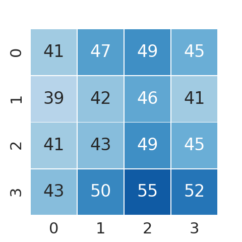
(e) 25% - ES-(1+1)

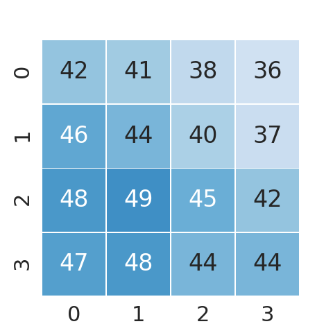
(f) 50% - ES-(1+1)

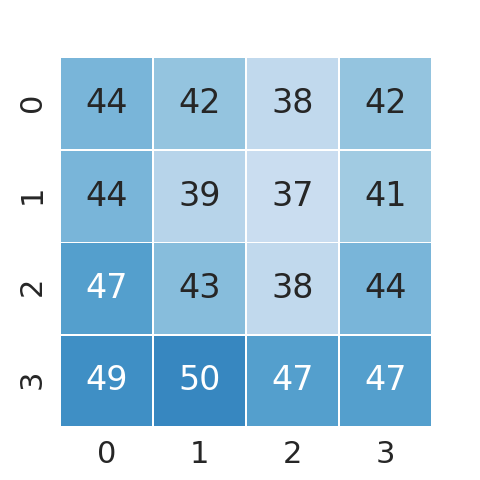
(g) 75% - ES-(1+1)

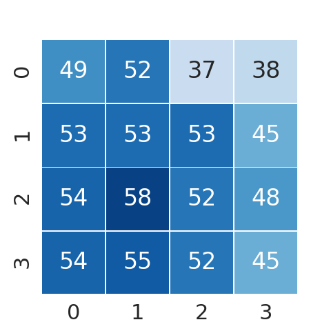
(h) 100% - ES-(1+1)

Figure 5: FID score distribution through a given grid at the end of an independent run for MNIST-4$\times$4. Lighter blues represent lower (better) FID scores. The first row (a, b, c, and d) illustrates the FIDs of each ensemble by using uniform mixture weights. The third row (e, f, g, and h) shows the FIDs of each ensemble by using the weights computed by the ES-(1+1).

6 Conclusions and Future Work

The use of less training data reduces the storage requirements, both disk and RAM while depending on the ensemble of generators to limit possible loss in performance from the reduction of training data. In the case of Redux-Lipizzaner there is also the potential benefit of the implicit communication that comes from the training on overlapping neighborhoods and updating the cell with the best generator after a training epoch. Our method, Redux-Lipizzaner, for spatially distributed evolutionary GAN training makes use of information exchange between neighborhoods to generate high performing generator mixtures. The spatially distributed grids allow training with less of the dataset because of signal propagation leading to exchange of information and improved performance when training data is reduced compared to ordinary parallel GAN training. In addition, the ensembles lose performance when the training data is reduced, but they are surprisingly robust with 75% of the data.

Future work will investigate the impact of distributing different modes(e.g. classes) of the data to different cells. In addition, more data sets will be evaluated, as well as more fine grained reductions in amount of training data.

References

- (1) Morse et al., G.: Simple evolutionary optimization can rival stochastic gradient descent in neural networks. In: GECCO, pp. 477–484. ACM (2016)
- (2) Al-Dujaili, A., Schmiedlechner, T., Hemberg, E., O’Reilly, U.M.: Towards distributed coevolutionary GANs. In: AAAI 2018 Fall Symposium (2018)
- (3) Al-Dujaili, A., Srikant, S., Hemberg, E., O’Reilly, U.M.: On the application of Danskin’s theorem to derivative-free minimax optimization. Int. Workshop on Global Optimization (2018)
- (4) Ambrogioni, L., Güçlü, U., van Gerven, M.: k-gans: Ensemble of generative models with semi-discrete optimal transport. ArXiv abs/1907.04050 (2019)
- (5) Arnaldo, I., Veeramachaneni, K., Song, A., O’Reilly, U.M.: Bring your own learner: A cloud-based, data-parallel commons for machine learning. IEEE Computational Intelligence Magazine 10(1), 20–32 (2015)
- (6) Arora, S., Ge, R., Liang, Y., Ma, T., Zhang, Y.: Generalization and equilibrium in generative adversarial nets (gans). arXiv preprint arXiv:1703.00573 (2017)
- (7) Arora, S., Risteski, A., Zhang, Y.: Do GANs learn the distribution? some theory and empirics. In: International Conference on Learning Representations (2018). URL https://openreview.net/forum?id=BJehNfW0-
- (8) Grover, A., Ermon, S.: Boosted generative models. ArXiv abs/1702.08484 (2017)
- (9) Hardy, C., Merrer, E.L., Sericola, B.: Md-gan: Multi-discriminator generative adversarial networks for distributed datasets. 2019 IEEE International Parallel and Distributed Processing Symposium (IPDPS) pp. 866–877 (2018)
- (10) Herrmann, J.W.: A genetic algorithm for minimax optimization problems. In: CEC, vol. 2, pp. 1099–1103. IEEE (1999)
- (11) Heusel, M., Ramsauer, H., Unterthiner, T., Nessler, B.: Gans trained by a two time-scale update rule converge to a local nash equilibrium. arXiv preprint arXiv:1706.08500 (2017)
- (12) Heusel, M., Ramsauer, H., Unterthiner, T., Nessler, B., Klambauer, G., Hochreiter, S.: GANs trained by a two time-scale update rule converge to a nash equilibrium. arXiv preprint arXiv:1706.08500 12(1) (2017)
- (13) Hillis, W.D.: Co-evolving parasites improve simulated evolution as an optimization procedure. Physica D: Nonlinear Phenomena 42(1), 228 – 234 (1990). DOI https://doi.org/10.1016/0167-2789(90)90076-2
- (14) Hodjat, B., Hemberg, E., Shahrzad, H., O’Reilly, U.M.: Maintenance of a long running distributed genetic programming system for solving problems requiring big data. In: Genetic Programming Theory and Practice XI, pp. 65–83. Springer (2014)
- (15) Husbands, P.: Distributed coevolutionary genetic algorithms for multi-criteria and multi-constraint optimisation. In: AISB Workshop on Evolutionary Computing, pp. 150–165. Springer (1994)
- (16) LeCun, Y.: The mnist database of handwritten digits. http://yann. lecun. com/exdb/mnist/ (1998)
- (17) Li, J., Madry, A., Peebles, J., Schmidt, L.: Towards understanding the dynamics of generative adversarial networks. arXiv preprint arXiv:1706.09884 (2017)
- (18) Liu, Z., Luo, P., Wang, X., Tang, X.: Deep learning face attributes in the wild. In: Proceedings of International Conference on Computer Vision (ICCV) (2015)
- (19) Loshchilov, I.: Surrogate-assisted evolutionary algorithms. Ph.D. thesis, University Paris South Paris XI; National Institute for Research in Computer Science and Automatic-INRIA (2013)
- (20) Mitchell, M.: Coevolutionary learning with spatially distributed populations. Computational Intelligence: Principles and Practice (2006)
- (21) Salimans, T., Ho, J., Chen, X., Sutskever, I.: Evolution strategies as a scalable alternative to reinforcement learning. arXiv:1703.03864 (2017)
- (22) Stanley, K.O., Clune, J.: Welcoming the era of deep neuroevolution - uber engineering blog. https://eng.uber.com/deep-neuroevolution/ (2017)
- (23) Tolstikhin, I.O., Gelly, S., Bousquet, O., Simon-Gabriel, C.J., Schölkopf, B.: Adagan: Boosting generative models. In: NIPS (2017)
- (24) Toutouh, J., Hemberg, E., O’Reilly, U.M.: Spatial evolutionary generative adversarial networks. In: GECCO (2019)
- (25) Wang, C., Xu, C., Yao, X., Tao, D.: Evolutionary generative adversarial networks. arXiv preprint arXiv:1803.00657 (2018)
- (26) Wang, Y., Zhang, L., van de Weijer, J.: Ensembles of generative adversarial networks. ArXiv abs/1612.00991 (2016)
- (27) Wierstra, D., Schaul, T., Peters, J., Schmidhuber, J.: Natural evolution strategies. In: Evolutionary Computation, 2008. CEC 2008.(IEEE World Congress on Computational Intelligence). IEEE Congress on, pp. 3381–3387. IEEE (2008)
- (28) Williams, N., Mitchell, M.: Investigating the success of spatial coevolution. In: Proceedings of the 7th annual conference on Genetic and evolutionary computation, pp. 523–530. ACM (2005)
- (29) Zhong, P., Mo, Y., Xiao, C., Chen, P., Zheng, C.: Rethinking generative coverage: A pointwise guaranteed approach. ArXiv abs/1902.04697 (2019)