Noisy three-player dilemma game: Robustness of the quantum advantage

Abstract

Games involving quantum strategies often yield higher payoff. Here, we study a practical realization of the three-player dilemma game using the superconductivity-based quantum processors provided by IBM Q Experience. We analyze the persistence of the quantum advantage under corruption of the input states and how this depends on parameters of the payoff table. Specifically, experimental fidelity and error are observed not to be properly anti-correlated, i.e., there are instances where a class of experiments with higher fidelity yields a greater error in the payoff. Further, we find that the classical strategy will always outperform the quantum strategy if corruption is higher than half.

1 Introduction

Game theory provides a way to learn about decisive communication between rational and self-seeking agents. Therefore, it plays an important role in the fields of computer science, economics, biology, psychology, etc. (see [1, 2] for review). Computationally, game theory can be used to model algorithms [3, 4] as well as check the robustness of networks and corresponding attack strategies [5]. In cryptography, the communication task can be visualized as a game between the parties trying to communicate securely and an eavesdropper ([6] and references therein). With the advent of quantum computing, it is observed that resources used in quantum computing, such as quantum coherence and entanglement, provide alternative solutions to classical games.

We may mention, for example, the emergence of cooperation in the prisoner’s dilemma game [7] and the resolution of the coordination in battle of sexes game [8] using entanglement. Specifically, as all the players wish to maximize their gain or payoff in games, for which the umpire has laid down the rule(s), players using quantum mechanical tactics are found to attain a higher payoff compared to the classical one [9]. Further, the dilemma disappears in prisoner’s dilemma with the use of quantum resources under unitary operations [10, 11]. Along the same line, optimal cloning of quantum states is also studied as game [12]. Quantum games based on monogamy of entanglement are shown to be useful in device independent quantum cryptography [13]. Our understanding of several other foundational aspects of quantum mechanics is improved by considering games, such as nonlocality [14], the uncertainty bound on nonlocality [15], contextuality [16], PR-boxes [17], as well as applications in quantum reinforcement learning [18] and quantum machine learning [19].

Over the course of time, multiplayer quantum games were also introduced that exploit quantum correlation to prevent betrayal by individual players [20]. It has been suggested that these quantum games may shed light on the interactions in many-particle systems [21]. One such multiplayer game is the three-party counterpart of the prisoner’s dilemma. In the classical version, all three players prefer to choose analogous to the corresponding two-party case. The dilemma exists because the Nash equilibrium does not coincide with the Pareto optimal [20]. Specifically, a Nash equilibrium is the situation in which no participant can gain by a unilateral change of strategy, while Pareto optimal corresponds to the situation that any change in strategy would make at least one individual worse off [20]. Still in quantum case, use of tripartite entanglement shows certain advantage. Moreover, computing the Nash equilibrium in the three- and four- player games is shown to be a hard problem [22, 23]. An experimental verification of three-player dilemma game using NMR was reported in Ref. [24]. In the recent past, other games have been realized on photonic quantum computer [25, 26, 27, 28] and ion trap platform [29].

In general, the dilemma games are relevant in several studies of biology, economics, psychology, international relations, sports to name a few. For instance, King Solomon’s dilemma [30] based on the Old Testament can model prize allocation, research grant distribution, etc. Another multiparty version of prisoner’s dilemma is diner’s dilemma in which each player has to choose whether to order an expensive or an inexpensive dish if they have to equally share the bill [31]. This iterated diner’s dilemma is useful in the social dynamics of networks and situational awareness. Such iterated multiparty prisoner’s dilemma in the context of social dynamics is discussed in the past, too [32]. Along the same line, dilemma of the players in other games is used to introduce the conditional probability [33].

Decoherence is the Achilles’ heel of quantum computing and information processing in particular, and technology in general. Similar results are shown for the quantum games [34]. Independently, the effect of errors in the initial state preparation (as corruption by a demon) on the outcome of three-player dilemma game is studied assuming that the players are unaware of corruption and that there is no decoherence [21]. Interestingly, beyond a pivotal value of corruption it can be observed that players fare off better with the classical strategies, but since players have no knowledge of the level of corruption they have to stick to their original strategies. Furthermore, a quantum game reduces to classical game if one of the parties allows his qubit to decohere under Markovian noise channels [35], while Nash equilibria are unchanged by decoherence for prisoner’s dilemma [36].

Here, we wish to implement the three-player dilemma game [20] on IBM quantum computer [37] and study how the change in the utility function affects the point of quantum advantage. Interestingly, this is the first realization of a game with corrupt source on a superconducting qubits based quantum computer. Despite high error rate and the limited qubit connectivity, it has been shown to run a wide array of algorithms ([38, 39] and references therein). Thus, we realize the game on IBM Q Experience and compare the experimental payoffs with previous experiments on NMR [24]. On generalizing the payoff table in the noisy game, the point where quantum advantage disappears also changes which leads to some interesting observations. In specific, they show how robust the quantum strategy is. An application of these results is that given a known corruption level, the payoff table (the relative stakes) may, in a range, be chosen to give an advantage to the quantum strategy. Finally, we show that classical strategies dominate when corruption is higher than 50% in the proposed game.

The rest of the paper is organized as follows. We introduce three-player quantum dilemma in Section 2. The noisy counterpart of the game and its experimental implementation is discussed in Section 3. We further discuss all the results in detail in the penultimate section before concluding the paper in Section 5.

2 Three-person quantum dilemma

A multiparty dilemma game was introduced as a multiparty counterpart of the prisoner’s dilemma game, where each person has two choices: either to cooperate (0) or defect (1). The three-player dilemma resembles el-Farol bar problem that players have to decide independently whether to go or not to a bar with seating capacity for only two ([24] and references therein).

In the three-player quantum dilemma game, each player is provided one qubit by the umpire, who performs an entangling operation on state $\left|000\right\rangle$ before that which increases the nonclassical correlation among the players. The entangling gate $J$ can be defined as in Ref. [20]:

$$J=\cos\frac{\gamma}{2}I^{\varotimes 3}+i\sin\frac{\gamma}{2}X^{\varotimes 3},$$ (1)

where $I$ and $X$ are identity and Pauli NOT gates, respectively. Without loss of generality, we choose the case when the correlation is maximum, i.e., $\gamma=\pi/2$. Further, it can be checked that for minimum correlation, i.e., $\gamma=0$, the game reduces to its classical counterpart [11].

In quantum game, each person is allowed to choose an operation from a strategy set $S$, consisting of 3 elements $S=(S_{1},S_{2},S_{3})$, where $S_{1}=X$ means the player wants to attend the party; $S_{2}=H$ corresponds to the player’s choice to go with half a probability; and $S_{3}=I$ represents the player wants to stay at home. Note that the choice of $S_{2}$ does not have a counterpart in classical games. This is a restricted strategy set (as there can be an infinitely many possible quantum strategies each corresponding to a different unitary operation), but it encompasses all the nonclassical characteristics we want to demonstrate through this game. Subsequently, a disentangling operation $J^{\dagger}=\frac{I^{\varotimes 3}-iX^{\varotimes 3}}{\sqrt{2}}$ is performed before measuring in the computational basis. The circuit diagram of the game is shown in Fig. 1.

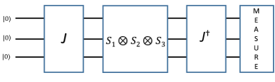
Figure 1: (Color online) Circuit diagram that can be used for the realization of the three-player quantum dilemma game.

Thus, when none of the players decide to go, i.e., the measurement outcome is $\left|000\right\rangle$ (represented by corresponding bit values 000 in Table 1), nobody is happy since they could not attend the party but are not sad since none of the friends betrayed, and thus everybody gets $0$ payoff. However, if one person decides to go then the other two will be unhappy (with payoff $-n$), and the one attending the party does not enjoy being alone (with payoff $p$). When two of the friends decide to go they both fare off with $n$ payoff each since they get to go to the party with company, while the friend left behind is not too dejected since his presence would have overcrowded the party so he gets $p$. If all of them decide to go, they get payoff of $q$ each since their presence has overcrowded the party. Accordingly, we impose $n>q>p>0$. This problem is also relevant in the recent pandemic coronavirus situation that may allow a restaurant to open but to avoid infection it restricts people who can sit at a table to two, say because the table is 1 m wide and only two persons can sit in the same table opposite to each other without violating the social distancing norms.

Yet another example for the three-player dilemma closer to most of us would be the dilemma of three academic collaborators in applying for a research grant. If two of them apply, they are likely to receive the grant, whereas they probably would receive insufficient or no funding if all three apply for it. Also, they would not be happy if none of them apply or their collaborator gets it but not them. The dilemma shown previously was by considering $n=9,\,p=1,$ and $q=2$ [20]. Here, we study a general description of such payoff tables and show how the payoff depends on these parameters in the noisy game (subjected to constraint $0<p<q<n$). One motivation for this is to understand whether and how the game’s stakes can be fixed based on knowledge of the preparation noise in the system. In [20], it is shown that in a special case considering a different set of values of the payoffs, quantum players do not have any advantage over the classical strategy which is no longer a Nash equilibrium. Therefore, we have restricted ourselves to the aforementioned constraint which ensures that classical Nash equilibrium exists. To the best of our knowledge, this is the first attempt to generalize the payoff table for the three-player dilemma game in analogy of prisoner’s dilemma [40].

Bit values corresponding to possible measurement outcome	Payoffs $\left(\$\right)$
000	$0,0,0$
001	$-n,-n,p$
010	$-n,p,-n$
011	$p,n,n$
100	$p,-n,-n$
101	$n,p,n$
110	$n,n,p$
111	$q,q,q$

Table 1: Generalized payoff table for three-player dilemma game depending upon the possible measurement outcomes. In previous adaptations of the game [20], $n=9,\,p=1,$ and $q=2$ were used.

3 IBM implementation and noisy state preparation

For the given strategy space $S$, there are 3 choices per player which gives us $3^{3}=27$ arrangements which can be clustered into 10 different classes [21]. Experimental design for the implementation of all these classes is shown in Fig. 2. Classes I, IV, and V have  ${3\choose 3}=1$  configuration, while Classes II, III, VI, VII, IX and X each have ${3\choose 1}=3$ possible configurations, and there are $3!=6$ configurations in Class VIII. When each player decides to play a unique tactic, independent of the other players, we obtain class VIII as mixed strategy Nash Equilibrium. Class VII provides best response for each player but is not considered as it is biased. Suppose the umpire has provided tainted qubits from the black box, i.e., instead of $\left|000\right\rangle$ he introduces error (mixedness) of the form $(1-x)\left|000\right\rangle\left\langle 000\right|+x\left|111\right\rangle\left\langle 111\right|$. The expected payoff would change quite exorbitantly as we increase the amount of preparation noise or corruption (as shown in Fig. 6), where $\text{\textquoteleft}x$’ is the noise parameter, $x\in[0,1]$.

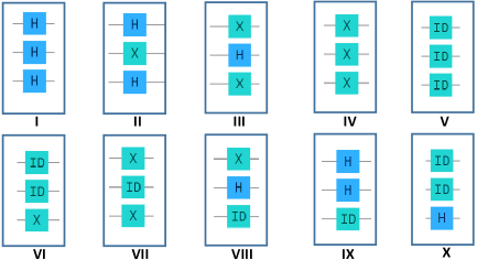
Figure 2: (Color online) Ten classes with different operations used by each player in $S_{1}\otimes S_{2}\otimes S_{3}$. Here, $H$, $X$, and ${\rm ID}$ are Hadamard, NOT, and identity gates, respectively.

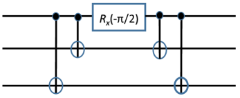
Figure 3: (Color online) Decomposition of three qubit operation $J$.

In IBM implementation [41] of the gate [42], we performed the entangling gate $J$ using a $R_{x}(-\frac{\pi}{2})$ and 4 CNOT gates as

$$J=\left(I_{0}\otimes CNOT_{1\rightarrow 2}\right)\,\left(CNOT_{1\rightarrow 0}\otimes I_{2}\right)\,\left(I_{0}\otimes R_{x}\left(-\frac{\pi}{2}\right)_{1}\otimes I_{2}\right)\,\left(I_{0}\otimes CNOT_{1\rightarrow 2}\right)\,\left(CNOT_{1\rightarrow 0}\otimes I_{2}\right)$$

on qubits 0, 1, and 2, respectively (also shown in the Fig. 3). The single qubit operation can be defined as $R_{x}(-\frac{\pi}{2})\left|0\right\rangle\rightarrow\left(\left|0\right\rangle+i\left|1\right\rangle\right)/\sqrt{2}$. In fact, many simulations of this game have modeled the entangling gate $J$ incorrectly in the past [42] as those matrix decomposition were not the same as $J$. As already discussed this is followed by the players applying their operations on their respective qubits from the strategy space $S$. Finally, we apply a disentagling gate $J^{\dagger}$ which can be modeled by the same gates as $J$ since $(ABCDE)^{\dagger}=E^{\dagger}D^{\dagger}C^{\dagger}B^{\dagger}A^{\dagger}$.

To introduce the corruption in the input qubits (shown in Fig. 4), the umpire uses an ancilla in state $\left|\psi\right\rangle=U(\theta,\phi,\lambda)\left|0\right\rangle=\cos\frac{\theta}{2}\left|0\right\rangle+\sin\frac{\theta}{2}\left|1\right\rangle$ prepared using single qubit unitary operation $U(\theta,\phi=0,\lambda=0)$ defined as

$$U(\theta,\phi,\lambda)=\left(\begin{array}[]{cc}\cos\frac{\theta}{2}&-e^{i\lambda}\sin\frac{\theta}{2}\\ e^{i\phi}\sin\frac{\theta}{2}&e^{i\lambda+i\phi}\cos\frac{\theta}{2}\end{array}\right).$$ (2)

Subsequently, he uses this ancilla as control and applies CNOT gates to the rest of the qubits which he sends to three players. The amount of corruption, $x$ is related by $x=\sin^{2}\frac{\theta}{2}$. Therefore, in what follows, we trace out the fourth qubit to obtain the payoffs of noisy game.

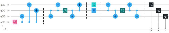
Figure 4: (Color online) Circuits for the simulation of noisy three-player quantum dilemma game for Class VIII as implemented on IBM Quantum Experience.

4 Results and discussion

We have performed the experiments for all classes and computed payoff from the measurement outcomes in computational basis. We have also obtained the output density matrices to obtain the fidelity between theoretically desired and experimentally reconstructed states.

4.1 Fidelity and quantum state tomography

In quantum computation, fidelity is used to describe closeness between two states as it is one of the distance based measures. Ideally, fidelity between the experimental ($\rho^{E}$) and theoretical ($\sigma$) density matrices, defined as $F(\rho^{E},\sigma)=Tr\sqrt{(\sqrt{\sigma}\rho^{E}\sqrt{\sigma)}}$ [39], is desired to be 1, but due to unavoidable errors it is usually less than unity in most cases.

In our case, we have calculated fidelities of all the classes and shown them in Table 2. To obtain the experimental density matrices and fidelities we performed quantum state tomography of the outputs of all the circuits (see [43, 44] for detail). The crux of the matter, is that we can reconstruct the three qubit density matrix of the output of the circuit using

$$\rho^{E}=\frac{1}{2^{3}}\stackrel{{\scriptstyle[}}{{i}}_{1},i_{2},i_{3}=0]{3}{\sum}T_{i_{1}i_{2}i_{3}}(\sigma_{i_{1}}\varotimes\sigma_{i_{2}}\varotimes\sigma_{i_{3}}),$$ (3)

where $\sigma_{j}$ are respective Pauli matrices. The values of elements of the $T$ matrix are obtained from the expectation values of these Pauli operators. For instance, in the case of Class VII, $U_{7}=\sigma_{x}\varotimes I\varotimes\sigma_{x}$ is the strategy unitary, the experimentally reconstructed density matrix is shown with corresponding theoretical density matrix $\sigma=\left|101\right\rangle\left\langle 101\right|$ in Fig. 5. The fidelity of the output density matrices for all the classes are summarized in Table 2. Surprisingly, fidelity and error are not properly anti-correlated, i.e., there are instances where a class of higher fidelity than another, still yields a greater error in the payoff. Here it may be noted that the experiments are performed on different processors provided by IBM depending upon their availability.

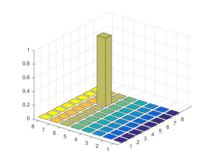
(a)

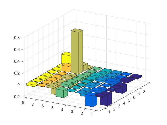
(b)

Figure 5: (Color online) Graphical representation of (a) the theoretical and (b) the real part of the experimentally reconstructed density matrices for Class VII.

Action	Theoretical	Experimental (IBM)	Experimental (NMR)	Fidelity	Error in Payoff(%)	Processor
Class I	-3.75	-2.7689	-3.65	0.6753	26	vigo
Class II	-3.75	-2.751	-3.44	0.7813	26.64	ourense
Class III	-1.833	-0.7384	-1.59	0.844	59.71	ourense
Class IV	2	2.3275	1.26	0.9236	16.3	ourense
Class V	0	-0.0676	0.4	0.9346	6.76	essex
Class VI	-5.67	-4.608	-5.39	0.9317	18.73	ourense
Class VII	6.33	4.459	5.92	0.843	29.5	ibmqx2
Class VIII	6.33	4.03	6.34	0.8416	36.3	ibm_16_melbourne
Class IX	4.75	3.2	4.83	0.6753	32.6	ibmqx2
Class X	-1.833	-0.8098	-1.87	0.6314	55.8	vigo

Table 2: Results of the experiments performed using different quantum processors in IBM Q Experience for the payoff table parameters $p=1,n=9,q=2$ considering state $x=0$. Surprisingly, fidelity and error are not properly anti-correlated, i.e., there are instances where a class of higher fidelity than another, still yields a greater error in the payoff. An example here for different processors would be Class III and Class I. Another example, for the same processor, would be, Classes IV and VI. A possible explanation could be noise during readout of payoffs.

4.2 Payoff table

Payoff of single player $\$$ is obtained by multiplying their respective payoffs from Table 1 with the probabilities obtained from the output of the experiment (as in [24]). The mean payoff per player $\left\langle\$\right\rangle$ is defined as the numerical mean of the payoffs of each player $\left\langle\$\right\rangle=\frac{\$1+\$2+\$3}{3}$.

It is also shown in the past that the payoffs for quantum Nash equilibrium deteriorate with noise [21]. However, in our case, assuming arbitrary values of parameters we obtained that quantum Nash equilibrium is $3\$_{{\rm qu}}=-4nx+2n+p$, and classical Nash equilibrium for ($q$,$q$,$q$) is $\$_{{\rm cl}}=q\left(1-x\right)$. As both quantum and classical Nash equilibrium values decrease with corruption level $x$, the quantum advantage disappears after the point of intersection of these two curves. That intersection can be obtained as the critical value of corruption

$$x_{c}=\frac{2n+p-3q}{4n-3q}.$$ (4)

From Fig. 6, we obtained that experimentally $x_{c}=0.363$ whereas the theoretical value is $0.428$ [21], giving us an error of $15.18\%$. Note that the results obtained in [21] neglect decoherence after the initial state is prepared by the demon. However, here on top of that, gate errors in the implementation of the presently available SQUID based quantum computing facilities also play an important role in sabotaging the quantum advantage achievable in quantum games. Of course, a reduction in noise with improvement in technology will improve the outcome. Notice that for very high values of corruption, when classical strategy is a preferred choice, the experimental results show higher payoffs than theoretically expected in quantum Nash equilibrium. The experimental values of payoff can be improved using mitigated error method provided by IBM.

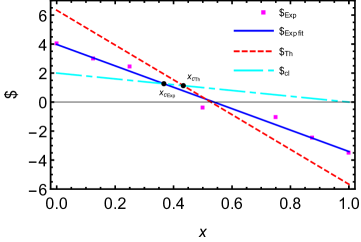
Figure 6: (Color online) Variation of payoffs in classical and quantum Nash equilibrium with corruption $x$. We have also shown the experimentally obtained payoff values. We assumed $p=1,\,n=9,$ and $q=2$. Here, $x_{c_{{\rm Th}}}$ and $x_{c_{{\rm Exp}}}$ represent critical values of corruption from theoretical and experimental results. Noise degrades quantum information, and thus not surprisingly, $x_{c_{{\rm Th}}}>x_{c_{{\rm Exp}}}$.

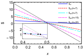
(a)

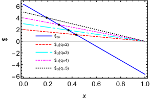
(b)

Figure 7: (Color online) Variation of payoffs in classical and quantum strategies with corruption $x$ and payoff parameters (a) $n$ ($q=2$) and (b) $q$ ($n=9$) with $p=1$ for Class VIII considering rest of the parameters in $\left\{p,n,q\right\}$ as constant. The critical value of corruption $x_{c}$ is marked by black dots in all cases.

4.3 Variation in $\boldsymbol{p,q,n}$

As we have discussed the general case of the game with arbitrary values of the individual payoff parameters, here we discuss the role of each of these parameters (assuming $0<p<q<n$) on $x_{c}$. This would allow us to choose suitable payoff parameters if the noise level $x$ is known, or if they cannot be varied, then to decide whether to employ the quantum or classical game for the problem in a practical situation.

We find that $x_{c}$ increases (shifts to the right of the original value) if $n$ is increased for a constant value of $p$ and $q$. It implies that when the stakes of a game are high (large $n$), such that reward for winnings and the amount of losses are very high, the quantum strategies are better in spite of corruption. Further increasing $n$ saturates $x_{c}$ to 0.5, which signifies that no matter what, if corruption is higher than 50% classical strategy will always outperform the quantum strategy. The results obtained are shown in Fig. 7 (a).

Note that the only quantum Nash equilibrium depends upon $n$, while classical Nash equilibrium is a function of $q.$ Thus, an increase in $q$ essentially leads to classical dominant strategy, i.e., classical strategy tends to be as efficient as the quantum strategy (cf. in Fig. 7 (b)). However, for large values of corruption there is no evident advantage as for maximum corruption classical Nash equilibrium is always zero.

These observation lead to conclusion that quantum systems are more prone to errors and deteriorate rapidly with an increase in the amount of corruption. Hence, errors in system may lead to loss of quantum advantage originally present as observed from the experimental value in Fig. 6 as well. Thus, in case of high errors, it is always better to stick to classical strategies from an outsider’s perspective.

5 Conclusion

We have discussed a multiparty quantum game by generalizing the payoff table. Our result may find interesting applications in diverse fields, such as finance, social networks. Suppose a group of companies want to invest in a particular stock and have limited knowledge of the market statistics, then the financial situation of the stock simulates a three-person dilemma. In this case, if the stakes of the investments are high such that returns are great, but so are the losses, companies perform better if they use quantum strategies, provided the amount of preparation noise is less than 50%. Otherwise the classical strategy should be preferred. Similarly, in the situation that the classical dominant strategy equilibrium $(q,q,q)$ has relatively higher payoff than previous cases, the present results may persuade companies to opt for classical strategies even for a small amount of source error.

We have performed an experiment for the noisy three-player quantum dilemma game and observed that the obtained results were less robust against noise than the corresponding results from NMR experiments. Further, it can be observed that due to additional errors (other than source error introduced in the noisy counterpart of the game) the advantage of quantum game over corresponding classical game disappears quickly. Similar studies for the generalizations of other games where quantum players perform better or the games where classical strategies are always preferable can be performed to study the role of various payoff parameters in those cases. The present experimental implementation of the noisy quantum game on a small noisy quantum computer establishes a practical quantum advantage in game theory. However, in view of noisy intermediate-scale quantum (NISQ) technology [45] around the corner, i.e., quantum computing infrastructure with 50-100 qubits, this advantage can be exploited for several applications, such as in quantum machine learning [46]. This can be further extended to the iterated version of the game where it is performed more than once, and rational players decide their strategies depending upon their opponents’ previous decision. The results from the experiment performed on NMR was more accurate, showing that the NMR-based quantum computer is less noisy. To obtain a quantitative perception of that we performed quantum state tomography here, which shows that higher fidelity of experimentally generated state does not necessarily mean smaller errors, i.e., fidelity and errors are not properly anti-correlated.

In the end, we would like to stress on the recent studies connecting Bell nonlocality [47, 48], a quantum secure direct communication scheme [49], and security of quantum key distribution schemes [50] with game theory. In view of these works, in principle, all quantum cryptographic schemes (see [51, 52] for a review) can be viewed from the perspective of game theory, as a game to perform cryptanalysis and obtain security proofs. For example, measurement-device-independent and device-independent as well as entangled state based quantum key distribution schemes, such as Ekert’s scheme [53], can be viewed as a three-party game involving Alice, Bob and Eve. A future work is planned to rigorously analyze the best strategy of Alice and Bob and that of Eve using a game theoretic approach. We hope the present results will be helpful in the application of quantum strategies in game theory, and in turn in their applications in quantum technologies in general, and quantum cryptography in particular.

Appendix: Reconstructed density matrix

The real and imaginary parts of the experimentally obtained density matrix by performing quantum state tomography are

$${\rm Re}(\rho^{E})=\left[\begin{array}[]{cccccccc}0.018&-0.188&-0.001&0.002&-0.126&0.036&-0.004&-0.031\\ -0.188&0.030&-0.100&0.002&0.044&-0.160&-0.019&-0.003\\ -0.001&-0.100&0.037&-0.003&0.033&-0.056&-0.049&-0.035\\ 0.002&0.002&-0.003&0.007&0.015&0.030&-0.042&-0.039\\ -0.126&0.044&0.033&0.015&0.022&-0.189&-0.006&-0.002\\ 0.036&-0.160&-0.056&0.030&-0.189&0.711&0.099&-0.030\\ -0.004&-0.019&-0.049&-0.042&-0.006&0.099&0.018&-0.022\\ -0.031&-0.003&-0.035&-0.039&-0.002&-0.030&-0.022&0.157\end{array}\right]$$

and

$${\rm Im}(\rho^{E})=\left[\begin{array}[]{cccccccc}0&0.229&0.002&0.009&0.142&-0.042&-0.028&-0.009\\ -0.229&0&0&-0.001&-0.001&0.148&-0.010&-0.034\\ -0.002&0&0&{0.002}&-0.011&0.014&0.053&0.010\\ -0.009&0.001&{-0.002}&0&0.014&0.017&0.004&0.030\\ -0.142&0.001&0.011&-0.014&0&{0.158}&0.004&-1.108\\ 0.042&-0.148&-0.014&-0.017&{-0.158}&0&-1.103&0.058\\ 0.028&0.010&-0.053&-0.004&-0.004&1.103&0&0.024\\ 0.009&0.034&-0.010&-0.030&1.108&-0.058&-0.024&0\end{array}\right],$$

respectively, while theoretical density matrix in the corresponding case is given by $\sigma=\left|\psi\right\rangle\left\langle\psi\right|=\left|101\right\rangle\left\langle 101\right|$, where $\left|\psi\right\rangle=J^{\dagger}\cdotp U_{7}\cdotp J\left|000\right\rangle$.

References

- [1] Flitney, A. P., Abbott, D.: An introduction to quantum game theory. Fluctuation and Noise Letters 2, R175–R187 (2002)
- [2] Piotrowski, E. W., Sładkowski, J.: An invitation to quantum game theory. International Journal of Theoretical Physics 42, 1089–1099 (2003)
- [3] Li, X., Gao, L., Li, W.: Application of game theory based hybrid algorithm for multi-objective integrated process planning and scheduling. Expert Systems with Applications 39, 288–297 (2012)
- [4] Elhenawy, M., Elbery, A. A., Hassan, A. A., Rakha, H. A.: An intersection game-theory-based traffic control algorithm in a connected vehicle environment. in: 2015 IEEE 18th international conference on intelligent transportation systems pp. 343–347 IEEE (2015)
- [5] Laszka, A., Szeszlér, D., Buttyán, L.: Game-theoretic robustness of many-to-one networks. in: International Conference on Game Theory for Networks pp. 88–98 Springer (2012)
- [6] Dodis, Y., Rabin, T., et al.: Cryptography and game theory. Algorithmic game theory pp. 181–207 (2007)
- [7] Li, A., Yong, X.: Entanglement guarantees emergence of cooperation in quantum prisoner’s dilemma games on networks. Scientific reports 4, 1–7 (2014)
- [8] Nawaz, A., Toor, A. H.: Dilemma and quantum battle of sexes. Journal of Physics A: Mathematical and General 37, 4437 (2004)
- [9] Meyer, D. A.: Quantum strategies. Physical Review Letters 82, 1052 (1999)
- [10] Eisert, J., Wilkens, M., Lewenstein, M.: Quantum games and quantum strategies. Physical Review Letters 83, 3077 (1999)
- [11] Du, J., Xu, X., Li, H., Zhou, X., Han, R.: Playing prisoner’s dilemma with quantum rules. Fluctuation and Noise Letters 2, R189–R203 (2002)
- [12] Werner, R. F.: Optimal cloning of pure states. Physical Review A 58, 1827 (1998)
- [13] Tomamichel, M., Fehr, S., Kaniewski, J., Wehner, S.: A monogamy-of-entanglement game with applications to device-independent quantum cryptography. New Journal of Physics 15, 103002 (2013)
- [14] Fritz, T., Sainz, A. B., Augusiak, R., et al.: Local orthogonality as a multipartite principle for quantum correlations. Nature communications 4, 1–7 (2013)
- [15] Oppenheim, J. and Wehner, S., 2010. The uncertainty principle determines the nonlocality of quantum mechanics. Science, 330(6007), pp.1072-1074.
- [16] Anshu, A., Høyer, P., Mhalla, M., Perdrix, S.: Contextuality in multipartite pseudo-telepathy graph games. Journal of Computer and System Sciences 107, 156–165 (2020)
- [17] Popescu, S.: Nonlocality beyond quantum mechanics. Nature Physics 10, 264–270 (2014)
- [18] Chen, C., Dong, D., Dong, Y., Shi, Q.: A quantum reinforcement learning method for repeated game theory. in: 2006 International Conference on Computational Intelligence and Security volume 1 pp. 68–72 IEEE (2006)
- [19] Clausen, J., Briegel, H. J.: Quantum machine learning with glow for episodic tasks and decision games. Physical Review A 97, 022303 (2018)
- [20] Benjamin, S. C., Hayden, P. M.: Multiplayer quantum games. Physical Review A 64, 030301 (2001)
- [21] Johnson, N. F.: Playing a quantum game with a corrupted source. Physical Review A 63, 020302 (2001)
- [22] Daskalakis, C., Papadimitriou, C. H.: Three-player games are hard. in: Electronic colloquium on computational complexity volume 139 pp. 81–87 (2005)
- [23] Daskalakis, C., Goldberg, P. W., Papadimitriou, C. H.: The complexity of computing a Nash equilibrium. SIAM Journal on Computing 39, 195–259 (2009)
- [24] Mitra, A., Sivapriya, K., Kumar, A.: Experimental implementation of a three qubit quantum game with corrupt source using nuclear magnetic resonance quantum information processor. Journal of Magnetic Resonance 187, 306–313 (2007)
- [25] Kolenderski, P., Sinha, U., Youning, L., et al.: Aharon-Vaidman quantum game with a Young-type photonic qutrit. Physical Review A 86, 012321 (2012)
- [26] Pinheiro, A., Souza, C., Caetano, D., et al.: Vector vortex implementation of a quantum game. JOSA B 30, 3210–3214 (2013)
- [27] Schmid, C., Flitney, A. P., Wieczorek, W., et al.: Experimental implementation of a four-player quantum game. New Journal of Physics 12, 063031 (2010)
- [28] Zhou, L., Kuang, L.-M.: Proposal for optically realizing a quantum game. Physics Letters A 315, 426–430 (2003)
- [29] Solmeyer, N., Linke, N. M., Figgatt, C., et al.: Demonstration of a Bayesian quantum game on an ion-trap quantum computer. Quantum Science and Technology 3, 045002 (2018)
- [30] Glazer, J., Ma, C.-t. A.: Efficient allocation of a “prize”-King Solomon’s dilemma. Games and Economic Behavior 1, 222–233 (1989)
- [31] Teng, Y., Jones, R., Marusich, L., et al.: Trust and situation awareness in a 3-player diner’s dilemma game. in: 2013 IEEE International Multi-Disciplinary Conference on Cognitive Methods in Situation Awareness and Decision Support (CogSIMA) pp. 9–15 IEEE (2013)
- [32] Bankes, S.: Exploring the foundations of artificial societies: Experiments in evolving solutions to iterated N-player prisoner’s dilemma. in: Artificial Life IV pp. 337–342 MIT Press Cambridge, MA (1994)
- [33] Morgan, J. P., Chaganty, N. R., Dahiya, R. C., Doviak, M. J.: Let’s make a deal: The player’s dilemma. The American Statistician 45, 284–287 (1991)
- [34] Özdemir, Ş. K., Shimamura, J., Imoto, N.: Quantum advantage does not survive in the presence of a corrupt source: optimal strategies in simultaneous move games. Physics Letters A 325, 104–111 (2004)
- [35] Chen, J.-L., Kwek, L. C., Oh, C. H.: Noisy quantum game. Physical Review A 65, 052320 (2002)
- [36] Chen, L., Ang, H., Kiang, D., Kwek, L., Lo, C.: Quantum prisoner dilemma under decoherence. Physics Letters A 316, 317–323 (2003)
- [37] IBM Q. https://www.research.ibm.com/ibm-q/. Accessed on September 2019
- [38] Sisodia, M., Shukla, A., Thapliyal, K., Pathak, A.: Design and experimental realization of an optimal scheme for teleportation of an n-qubit quantum state. Quantum Information Processing 16, 292 (2017)
- [39] Sisodia, M., Shukla, A., de Almeida, A. A., Dueck, G. W., Pathak, A.: Circuit optimization for IBM processors: A way to get higher fidelity and higher values of nonclassicality witnesses. arXiv preprint arXiv:1812.11602 (2018)
- [40] Tian, J., Uchida, N.: Monkeys in a prisoner’s dilemma. Cell 160, 1046–1048 (2015)
- [41] Shukla, A., Sisodia, M., Pathak, A.: Complete characterization of the directly implementable quantum gates used in the IBM quantum processors. arXiv preprint arXiv:1805.07185 (2018)
- [42] Sousa, P. B., Ramos, R. V.: Universal quantum circuit for n-qubit quantum gate: A programmable quantum gate. arXiv preprint quant-ph/0602174 (2006)
- [43] Sisodia, M., Shukla, A., Pathak, A.: Experimental realization of nondestructive discrimination of Bell states using a five-qubit quantum computer. Physics Letters A 381, 3860–3874 (2017)
- [44] Vishnu, P., Joy, D., Behera, B. K., Panigrahi, P. K.: Experimental demonstration of non-local controlled-unitary quantum gates using a five-qubit quantum computer. Quantum Information Processing 17, 274 (2018)
- [45] Preskill, J.: Quantum computing in the NISQ era and beyond. Quantum 2, 79 (2018)
- [46] Torlai, G., Melko, R.: Machine-learning quantum states in the NISQ era. Annual Review of Condensed Matter Physics 11 (2019)
- [47] Brunner, N., Linden, N.: Connection between Bell nonlocality and Bayesian game theory. Nature communications 4, 2057 (2013)
- [48] Iqbal, A., Chappell, J. M., Abbott, D.: The equivalence of Bell’s inequality and the Nash inequality in a quantum game-theoretic setting. Physics Letters A 382, 2908–2913 (2018)
- [49] Kaur, H., Kumar, A.: Game-theoretic perspective of ping-pong protocol. Physica A: Statistical Mechanics and its Applications 490, 1415–1422 (2018)
- [50] Krawec, W. O., Miao, F.: Game theoretic security framework for quantum key distribution. in: International Conference on Decision and Game Theory for Security pp. 38–58 Springer (2018)
- [51] Pathak, A.: Elements of quantum computation and quantum communication. Taylor & Francis, New York (2013)
- [52] Thapliyal, K., Pathak, A., Banerjee, S.: Quantum cryptography over non-Markovian channels. Quantum Information Processing 16, 115 (2017)
- [53] Ekert, A. K.: Quantum cryptography based on Bell’s theorem. Phys. Rev. Lett. 67, 661 (1991)