Rethinking the Mathematical Framework and Optimality of Set-Membership Filtering

Abstract

Set-Membership Filter (SMF) has been extensively studied for state estimation in the presence of bounded noises with unknown statistics. Since it was first introduced in the 1960s, the studies on SMF have used the set-based description as its mathematical framework. One important issue that has been overlooked is the optimality of SMF. In this work, we put forward a new mathematical framework for SMF using concepts of uncertain variables. We first establish two basic properties of uncertain variables, namely, the law of total range (a non-stochastic version of the law of total probability) and the equivalent Bayes’ rule. This enables us to put forward a general SMFing framework with established optimality. Furthermore, we obtain the optimal SMF under a non-stochastic Markov condition, which is shown to be fundamentally equivalent to the Bayes filter. Note that the classical SMF in the literature is only equivalent to the optimal SMF we obtained under the non-stochastic Markov condition. When this condition is violated, we show that the classical SMF is not optimal and it only gives an outer bound on the optimal estimation.

I Introduction

I-A Motivation and Related Work

The filtering problems in the state-space description are concerned with estimating the state information in the presence of noises, and thus are widely considered in control systems, telecommunications, navigation, and many other important fields [1, 2]. When the statistics of the noises are known, the corresponding solution method is called stochastic filter. A famous optimal filtering framework for Hidden Markov Models (HMMs) is the Bayes filter [1, 2, 3] which provides the complete solution to the filtering problem. As a special case, if the noises are white Gaussian in linear systems, the corresponding Bayes filter is known as the Kalman filter [4]. Note that in the Bayes filter, the white noise assumption plays an important role in supporting the optimality, since otherwise the HMM condition can hardly be guaranteed.

When the noises have unknown statistics but known ranges, the corresponding solution method is called non-stochastic filter. In the 1960s, Witsenhausen proposed a famous filtering framework for linear systems [5, 6], which is also suitable for nonlinear systems, known as the Set-Membership Filter (SMF). Similarly to the Bayes filter, the SMF also has the prediction step (using the set image under system function, which becomes the Minkowski sum for linear systems) and the update step (using the set intersection). Under this classical SMFing framework, the follow-up/existing studies focused on how to derive the exact or approximate solution for different scenarios. More specifically, there are mainly two types of SMFs in the literature:

• Ellipsoidal SMF. This type of SMFs approximates the Minkowski sum and set intersection using ellipsoidal outer bounds. In [10], a continuous-discrete ellipsoidal SMF was proposed to outer bound the estimate of the linear systems with two specific types of noises, which has a similar structure to the Kalman filter. With a similar system setting, both SMFing and smoothing problems were investigated in [11] by solving corresponding Riccati equations. In [12] and [13], algorithms were provided for minimizing the volume of the outer bounds on the Minkowski sum and intersection of ellipsoids. Nevertheless, minimizing the volume can result in a very narrow ellipsoid with an unacceptably large diameter. Thus, the semi-axes of ellipsoids were constrained, e.g., via the trace of the matrix in the quadratic form. In [14], a volume-minimizing and a trace-minimizing ellipsoidal outer bounds (each described by two ellipsoids) were derived for the linear discrete-time SMF, and the description of outer bounds were generalized to multiple ellipsoids in [15]. Note that the ellipsoidal SMF is computationally cheaper but usually less accurate than the polytopic SMF discussed below.

• Polytopic SMF. This type of SMFs describes or outer bounds the prediction and the update using convex polytopes. Different from the ellipsoidal SMF, the polytopic SMF can derive the exact solution for linear filtering problems, because polytopes are closed under Minkowski sum and set intersection. Nevertheless, the complexity is unacceptable for deriving exact solutions. Noticing this fact, researchers used different subclasses of convex polytopes to give the outer bounds. In [16], the recursive optimal bounding parallelotope algorithm was proposed to give an outer bound of the exact solution. In [17], a zonotopic SMF was designed for linear discrete-time systems by using singular-value-decomposition-based approximation. In [18], a zonotopic SMF was proposed for nonlinear discrete-time systems, where the zonotopic outer bound is derived by using convex optimization, which was improved in [19] by using the DC (Difference of two Convex functions) programming. In [20] and [21], the zonotopic SMFs were given for linear systems under P-radius-based and weighted-Frobenius-norm criteria, respectively, which efficiently balanced the complexity and the accuracy of the zonotopic outer bounds. In [22], the constrained zonotope was proposed and applied to the linear polytope-SMF, which can balance the complexity and the accuracy, and is closed under linear transformations, Minkowski sums, and set intersections. In [23], an SMF was proposed for nonlinear systems by combining the interval arithmetic and constrained zonotopes. In [24], a zonotopic SMF was studied for nonlinear systems which has advantages in handling high dimensionality.

All the above-mentioned studies on SMFs used the set-based description as its mathematical framework (see Remark 2 for a detailed discussion). We argue that this classical framework has the optimality issue: for stochastic filters, we know that even with the same marginal distributions, the white noises and correlated noises in linear systems lead to different Kalman filters [3]; for the SMFs, however, the noises with different non-stochastic correlations (which should result in different optimal estimations) were not distinguished; thus, the prior studies overlooked the condition (as shown later in Assumption 1) under which the SMFs are optimal, and the optimal SMFing framework has not been rigorously established. Departing from the classical/suboptimal set-based SMFing description, in this article, we aim to establish the optimal SMFing framework in a completely different way.

I-B Our Contributions

In this work, we put forward a new mathematical framework for SMFing, based on the concepts of uncertain variables proposed by Nair in the 2010s [25]. Similarly to the Bayesian filtering, our filtering framework recursively derives the non-stochastic prior and posterior. The main contributions are:

• We first establish two new and fundamental properties of uncertain variables: the first one is called the law of total range, which is a non-stochastic version of the law of total probability; the second one is the equivalent Bayes’ rule for uncertain variables. These properties enable us to define a new SMFing framework using the notion of uncertain variables.

• Most importantly, we establish an optimal SMFing framework that is more general than the well-known classical SMFing framework in the literature. With this new framework, we obtain the optimal SMF under an unrelatedness assumption (to guarantee a non-stochastic Markov condition), which is shown to be fundamentally equivalent to the Bayes filter. We also show that the classical SMFing framework in the literature is only optimal under this Markov condition, since it cannot capture the relatedness between the noises and the initial prior.

• Furthermore, we prove that when this Markoveness condition is violated, the classical SMFing gives an outer bound on the optimal estimation. We also use two examples to illustrate the performance gap between the classical SMFing framework in the literature and the optimal SMFing framework proposed in this work.

I-C Notation

Throughout this paper, $\mathbb{R}$, $\mathbb{N}_{0}$, and $\mathbb{Z}_{+}$ denote the sets of real numbers, non-negative integers, and positive integers, respectively. $\mathbb{R}^{n}$ stands for the $n$-dimensional Euclidean space.

II Uncertain Variables: Preliminaries and New Results

In this work, the uncertainties are with known ranges but unknown probability distributions. To model the uncertainties rigorously, we introduce the uncertain variable proposed in [25] and derive two important properties which will constitute the foundation of the optimal SMFing framework.

II-A Preliminaries of Uncertain Variables

Consider a sample space $\Omega$. A measurable function $\mathbf{x}\colon\Omega\to\mathcal{X}$ from the sample space $\Omega$ to a measurable set $\mathcal{X}$ is called an uncertain variable [25]. We define a realization of $\mathbf{x}$ as $\mathbf{x}(\omega)=:x$, and sometimes we write it as $\mathbf{x}=x$ for conciseness.

Different from random variables which can be described by probability distributions, an uncertain variable (say $\mathbf{x}$) does not have any information on the probability, but it can be described by its range $\llbracket\mathbf{x}\rrbracket$:

$$\llbracket\mathbf{x}\rrbracket:=\left\{\mathbf{x}(\omega)\colon\omega\in\Omega\right\}.$$ (1)

Similar to the probability distribution for multiple random variables, the range can also be defined w.r.t. multiple uncertain variables.

Definition 1 (Joint Range, Conditional Range, Marginal Range [25]).

Let $\mathbf{x}$ and $\mathbf{y}$ be two uncertain variables. The joint range of $\mathbf{x}$ and $\mathbf{y}$ is

$$\llbracket\mathbf{x},\mathbf{y}\rrbracket:=\left\{(\mathbf{x}(\omega),\mathbf{y}(\omega))\colon\omega\in\Omega\right\}.$$ (2)

The conditional range of $\mathbf{x}$ given $\mathbf{y}=y$ is

$$\llbracket\mathbf{x}|y\rrbracket:=\left\{\mathbf{x}(\omega)\colon\mathbf{y}(\omega)=y,\omega\in\Omega\right\}=\left\{\mathbf{x}(\omega)\colon\omega\in\Omega_{\mathbf{y}=y}\right\},$$ (3)

where $\Omega_{\mathbf{y}=y}:=\mathbf{y}^{-1}(\{y\})=\{\omega\colon\mathbf{y}(\omega)=y,\omega\in\Omega\}$ is the preimage of $\{\mathbf{y}(\omega)=y\colon\omega\in\Omega\}$, and $\llbracket\mathbf{y}|x\rrbracket$ is defined in a similar way. The marginal range of $\mathbf{x}$ is $\llbracket\mathbf{x}\rrbracket$ expressed by (1).

In analogy with the joint probability distribution, the joint range can be fully determined by the conditional and marginal ranges [25], i.e.,

$$\llbracket\mathbf{x},\mathbf{y}\rrbracket=\bigcup_{y\in\llbracket\mathbf{y}\rrbracket}\big{(}\llbracket\mathbf{x}|y\rrbracket\times\{y\}\big{)}=\bigcup_{x\in\llbracket\mathbf{x}\rrbracket}\big{(}\{x\}\times\llbracket\mathbf{y}|x\rrbracket\big{)},$$ (4)

where $\times$ is the Cartesian product.

Next, we introduce the definition of unrelatedness [25], which is a non-stochastic analogue of statistical independence.

Definition 2 (Unrelatedness and Conditional Unrelatedness [25]).

Uncertain variables $\mathbf{u}_{1},\ldots,\mathbf{u}_{r}$ are unrelated if

$$\llbracket\mathbf{u}_{1},\ldots,\mathbf{u}_{r}\rrbracket=\llbracket\mathbf{u}_{1}\rrbracket\times\cdots\times\llbracket\mathbf{u}_{r}\rrbracket.$$ (5)

They are conditionally unrelated given $\mathbf{v}$ if

$$\llbracket\mathbf{u}_{1},\ldots,\mathbf{u}_{r}|v\rrbracket=\llbracket\mathbf{u}_{1}|v\rrbracket\times\cdots\times\llbracket\mathbf{u}_{r}|v\rrbracket,\quad\forall v\in\llbracket\mathbf{v}\rrbracket.$$ (6)

If the uncertain variables are not unrelated, we say they are related. Based on Definition 2, we have the following properties for unrelatedness and conditional unrelatedness [25]:

• $\mathbf{u}_{1}$ and $\mathbf{u}_{2}$ are unrelated if and only if (iff)

  $$\llbracket\mathbf{u}_{1}|u_{2}\rrbracket=\llbracket\mathbf{u}_{1}\rrbracket,\quad\forall u_{2}\in\llbracket\mathbf{u}_{2}\rrbracket.$$ (7)

• $\mathbf{u}_{1}$ and $\mathbf{u}_{2}$ are conditionally unrelated given $v$ iff

  $$\llbracket\mathbf{u}_{1}|u_{2},v\rrbracket=\llbracket\mathbf{u}_{1}|v\rrbracket,\quad\forall(u_{2},v)\in\llbracket\mathbf{u}_{2},\mathbf{v}\rrbracket.$$ (8)

II-B Law of Total Range and New Bayes’ Rule

In this subsection, we establish two properties, namely, the law of total range and Bayes’ rule for uncertain variables, as the non-stochastic counterparts of the law of total probability and Bayes’ rule. They establish a mathematical foundation of the optimal SMF which will be introduced in Section III.

Lemma 1 (Law of Total Range).

$$\llbracket\mathbf{x}\rrbracket=\bigcup_{y\in\llbracket\mathbf{y}\rrbracket}\llbracket\mathbf{x}|y\rrbracket,\quad\llbracket\mathbf{y}\rrbracket=\bigcup_{x\in\llbracket\mathbf{x}\rrbracket}\llbracket\mathbf{y}|x\rrbracket.$$ (9)

Proof:

See Appendix A. ∎

The law of total range links the marginal range and the conditional range. An illustrative example is given in Fig. 1. With (9), we know that $\llbracket\mathbf{x}|y\rrbracket\subseteq\llbracket\mathbf{x}\rrbracket$ which implies observations can reduce uncertainty.

Lemma 2 (Bayes’ Rule for Uncertain Variables).

$$\llbracket\mathbf{x}|y\rrbracket=\left\{x\colon\llbracket\mathbf{y}|x\rrbracket\bigcap\{y\}\neq\emptyset,x\in\llbracket\mathbf{x}\rrbracket\right\}.$$ (10)

Proof:

See Appendix B. ∎

Bayes’ rule for uncertain variables reflects the fundamental relationship among the prior range $\llbracket\mathbf{x}\rrbracket$, the likelihood range $\llbracket\mathbf{y}|x\rrbracket$, and the posterior range $\llbracket\mathbf{x}|y\rrbracket$. An illustrative example is given in Fig. 1.

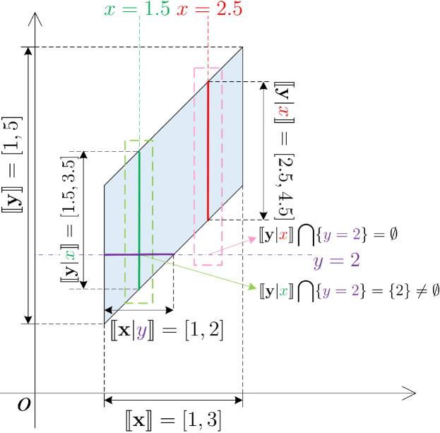
Figure 1: An illustrative example of the law of total range and Bayes’ rule for uncertain variables. The prior range is $\llbracket\mathbf{x}\rrbracket=[1,3]$, and the likelihood range is $\llbracket\mathbf{y}|x\rrbracket=\{x\}+[0,2]=[x,x+2]$. The law of total range (9) implies $\llbracket\mathbf{y}\rrbracket=\bigcup_{x\in\llbracket\mathbf{x}\rrbracket}\llbracket\mathbf{y}|x\rrbracket=[1,5]$ which can be verified easily in this figure. To illustrate how Bayes’ rule works, we take $\llbracket\mathbf{x}|y\rrbracket$ with $y=2$ (the purple dash-dotted line) for an example. When $x=1.5$ (the green dashed line), the likelihood range marked by the green solid line segment is $[1.5,3.5]$ which has a intersection with $y=2$, i.e., $\llbracket\mathbf{y}|x\rrbracket\bigcap\{y=2\}\neq\emptyset$. Thus, $x=1.5\in\llbracket\mathbf{x}|y\rrbracket$ for $y=2$. When $x=2.5$ (the red dashed line), the likelihood range marked by the red solid line segment is $[2.5,4.5]$ which has no intersections with $y=2$, i.e., $\llbracket\mathbf{y}|x\rrbracket\bigcap\{y=2\}=\emptyset$. Hence, $x=2.5\notin\llbracket\mathbf{x}|y\rrbracket$ for $y=2$. By applying Bayes’ rule to all $x\in\llbracket\mathbf{x}\rrbracket$, the posterior range $\llbracket\mathbf{x}|y\rrbracket=[1,2]$ marked by the purple solid line segment is obtained.

III The Optimal Filtering Framework

Now, we model the SMFing problem in the framework of uncertain variables. Consider the following nonlinear system:

$$\mathbf{x}_{k+1} =f_{k}(\mathbf{x}_{k},\mathbf{w}_{k}),$$ (11)

$$\mathbf{y}_{k} =g_{k}(\mathbf{x}_{k},\mathbf{v}_{k}),$$ (12)

for time $k\in\mathbb{N}_{0}$, where (11) and (12) are called the state equation and the measurement equation, respectively. The state equation describes how the system state $\mathbf{x}_{k}$ (with its realization $x_{k}\in\llbracket\mathbf{x}_{k}\rrbracket\subseteq\mathbb{R}^{n}$) changes over time, where $\mathbf{w}_{k}$ is the process/dynamical noise (with its realization $w_{k}\in\llbracket\mathbf{w}_{k}\rrbracket\subseteq\mathbb{R}^{p}$), and $f_{k}\colon\llbracket\mathbf{x}_{k}\rrbracket\times\llbracket\mathbf{w}_{k}\rrbracket\to\llbracket\mathbf{x}_{k+1}\rrbracket$ stands for the system transition function. The measurement equation gives how the system state is measured, where $\mathbf{y}_{k}$ represents the measurement (with its realization, called observed measurement, $y_{k}\in\llbracket\mathbf{y}_{k}\rrbracket\subseteq\mathbb{R}^{m}$) and $\mathbf{v}_{k}$ (with its realization $v_{k}\in\llbracket\mathbf{v}_{k}\rrbracket\subseteq\mathbb{R}^{q}$) stands for the measurement noise, and $g_{k}\colon\llbracket\mathbf{x}_{k}\rrbracket\times\llbracket\mathbf{v}_{k}\rrbracket\to\llbracket\mathbf{y}_{k}\rrbracket$ is the measurement function.

Now, we define the optimality criterion for SMF and then provide the optimal SMFing framework as follows.

Definition 3 (Optimal SMF).

An SMF is a process that $\forall k\in\mathbb{N}_{0}$, it gives an estimator $X_{k}(y_{0:k})$ that includes all possible $x_{k}$ given the measurements up to $k$, i.e., $y_{0:k}:=y_{0},\ldots,y_{k}$. An SMF is optimal if $X_{k}^{*}(y_{0:k})$ returns the smallest set such that $X_{k}^{*}(y_{0:k})\subseteq X^{\prime}_{k}(y_{0:k})$ holds for any $X^{\prime}_{k}$ and $y_{0:k}$.

Theorem 1 (Optimal Set-Membership Filtering Framework).

For the system described by (11) and (12), the optimal SMF is obtained by the following steps:

• Initialization. Set the initial prior range $\llbracket\mathbf{x}_{0}\rrbracket$.

• Prediction. For $k\in\mathbb{Z}_{+}$, given the posterior range $\llbracket\mathbf{x}_{k-1}|y_{0:k-1}\rrbracket$ in the previous time step, the prior range $\llbracket\mathbf{x}_{k}|y_{0:k-1}\rrbracket$ is predicted by the law of total range that

  $$\bigcup_{x_{k-1}\in\llbracket\mathbf{x}_{k-1}|y_{0:k-1}\rrbracket}\!\!\!\!\!\!\!\!\!\!\!f_{k-1}(x_{k-1},\llbracket\mathbf{w}_{k-1}|x_{k-1},y_{0:k-1}\rrbracket).$$ (13)

• Update. For $k\in\mathbb{N}_{0}$, given the observed measurement $y_{k}$ and the prior range $\llbracket\mathbf{x}_{k}|y_{0:k-1}\rrbracket$, the posterior range $\llbracket\mathbf{x}_{k}|y_{0:k}\rrbracket$ is updated by Bayes’ rule for uncertain variables that

  $$\!\!\left\{x_{k}\!\in\!\llbracket\mathbf{x}_{k}|y_{0:k-1}\rrbracket\colon g_{k}(x_{k},\llbracket\mathbf{v}_{k}|x_{k},y_{0:k-1}\rrbracket)\bigcap\{y_{k}\}\neq\emptyset\right\}$$ (14)

  where we define $\llbracket\mathbf{x}_{0}\rrbracket:=\llbracket\mathbf{x}_{0}|y_{0:-1}\rrbracket$ and $\llbracket\mathbf{v}_{0}|x_{0}\rrbracket=\llbracket\mathbf{v}_{0}|x_{0},y_{0:-1}\rrbracket$ for consistency.

Note that the posterior range obtained in (14) is the optimal estimator, i.e., $X_{k}^{*}(y_{0:k})=\llbracket\mathbf{x}_{k}|y_{0:k}\rrbracket$.

Proof:

See Appendix C. ∎

In general, it is not easy to obtain $\llbracket\mathbf{w}_{k-1}|x_{k-1},y_{0:k-1}\rrbracket$ and $\llbracket\mathbf{v}_{k}|x_{k},y_{0:k-1}\rrbracket$ in Theorem 1. They depend on how the process noises, the measurement noises, and the initial prior $\mathbf{w}_{0:k},\mathbf{v}_{0:k},\mathbf{x}_{0}$ are related. However, if the noises and the initial state are unrelated (see Assumption 1), the optimal filter is easy to derive (see Theorem 2).

Assumption 1 (Unrelated Noises and Initial State).

$\forall k\in\mathbb{N}_{0}$, $\mathbf{w}_{0:k},\mathbf{v}_{0:k},\mathbf{x}_{0}$ are unrelated.

Theorem 2 (Optimal SMFing Under Assumption 1).

For the system described by (11) and (12), the optimal SMF under Assumption 1 is given by the following steps:

• Initialization. Set the initial prior range $\llbracket\mathbf{x}_{0}\rrbracket$.

• Prediction. For $k\in\mathbb{Z}_{+}$, given $\llbracket\mathbf{x}_{k-1}|y_{0:k-1}\rrbracket$ derived in the previous time step $k-1$, the prior range is

  $$\llbracket\mathbf{x}_{k}|y_{0:k-1}\rrbracket=f_{k-1}(\llbracket\mathbf{x}_{k-1}|y_{0:k-1}\rrbracket,\llbracket\mathbf{w}_{k-1}\rrbracket).$$ (15)

• Update. For $k\in\mathbb{N}_{0}$, given the observed measurement $y_{k}$ and the prior range $\llbracket\mathbf{x}_{k}|y_{0:k-1}\rrbracket$, the posterior range is

  $$\llbracket\mathbf{x}_{k}|y_{0:k}\rrbracket=\!\!\left[\bigcup_{v_{k}\in\llbracket\mathbf{v}_{k}\rrbracket}g_{k,v_{k}}^{-1}(\{y_{k}\})\right]\bigcap\llbracket\mathbf{x}_{k}|y_{0:k-1}\rrbracket,$$ (16)

  where $g_{k,v_{k}}^{-1}(\cdot)$ is the inverse map of $g_{k}(\cdot,v_{k})$.

Proof:

See Appendix D. ∎

Remark 1 (Fundamental Equivalence Between SMF Under Assumption 1 and Bayes Filter).

The Bayes filter [1] is based on the stochastic Hidden Markov Model (HMM) with

$$p(x_{k}|x_{0:k-1},y_{0:k-1}) =p(x_{k}|x_{k-1}),$$ (17)

$$p(y_{k}|x_{0:k},y_{0:k-1}) =p(y_{k}|x_{k}),$$ (18)

where $p(a|b)$ is the conditional distribution of the random variable $\mathbf{a}$ given the realization $b=\mathbf{b}(\omega)$. For the optimal SMF, the system described by (11) and (12) under Assumption 1 satisfies the following non-stochastic HMM:

$$\llbracket\mathbf{x}_{k}|x_{0:k-1},y_{0:k-1}\rrbracket =\llbracket\mathbf{x}_{k}|x_{k-1}\rrbracket,$$ (19)

$$\llbracket\mathbf{y}_{k}|x_{0:k},y_{0:k-1}\rrbracket =\llbracket\mathbf{y}_{k}|x_{k}\rrbracket.$$ (20)

These two HMMs are equivalent, since $p(\cdot)$ and $\llbracket\cdot\rrbracket$ describe the uncertainties for random variables and uncertain variables, respectively. Furthermore, (17) reflects the conditional independence between $\mathbf{x}_{k}$ and $\mathbf{x}_{0:k-2},\mathbf{y}_{0:k-1}$ given $x_{k-1}$; while (19) indicates the conditional unrelatedness (8) between them. Similar observation can be obtained between (18) and (20).

In the Bayes filter, the prediction step is based on the Chapman-Kolmogorov equation, i.e., the law of total probability combined with the Markov property (17) that

$$p(x_{k}|y_{0:k-1})=\int p(x_{k}|x_{k-1})p(x_{k-1}|y_{0:k-1})\mathrm{d}x_{k-1}.$$ (21)

In the optimal SMF under Assumption 1, the prediction step is given by the law of total range (9) and the non-stochastic Markov property (19) that

$$\llbracket\mathbf{x}_{k}|y_{0:k-1}\rrbracket=\bigcup_{x_{k-1}\in\llbracket\mathbf{x}_{k-1}|y_{0:k-1}\rrbracket}\llbracket\mathbf{x}_{k}|x_{k-1}\rrbracket.$$ (22)

For the update steps, the Bayes filter derives the posterior distribution $p(x_{k}|y_{0:k})$ by Bayes’ rule, while the optimal SMF gets the posterior range $\llbracket\mathbf{x}_{k}|y_{0:k}\rrbracket$ by Bayes’ rule for uncertain variables (10).

Further, if the system is linear, the optimal SMFing under Assumption 1 is obtained in Corollary 1.

Corollary 1.

For the linear system described by

$$\mathbf{x}_{k+1} =A\mathbf{x}_{k}+B\mathbf{w}_{k},$$ (23)

$$\mathbf{y}_{k} =C\mathbf{x}_{k}+D\mathbf{v}_{k},$$ (24)

where $A\in\mathbb{R}^{n\times n}$, $B\in\mathbb{R}^{n\times p}$, $C\in\mathbb{R}^{m\times n}$, and $D\in\mathbb{R}^{m\times q}$, the optimal SMF under Assumption 1 has the following steps:

• Initialization. Set the initial prior range $\llbracket\mathbf{x}_{0}\rrbracket$.

• Prediction. For $k\in\mathbb{Z}_{+}$, the prior range is

  $$\llbracket\mathbf{x}_{k}|y_{0:k-1}\rrbracket=A\llbracket\mathbf{x}_{k-1}|y_{0:k-1}\rrbracket\oplus B\llbracket\mathbf{w}_{k-1}\rrbracket,$$ (25)

  where $\oplus$ stands for the Minkowski sum.

• Update. For $k\in\mathbb{N}_{0}$, given $y_{k}$, the posterior range is

  $$\llbracket\mathbf{x}_{k}|y_{0:k}\rrbracket=\mathcal{X}_{k}(C,y_{k},D\llbracket\mathbf{v}_{k}\rrbracket)\bigcap\llbracket\mathbf{x}_{k}|y_{0:k-1}\rrbracket,$$ (26)

  where we define $\llbracket\mathbf{x}_{0}\rrbracket:=\llbracket\mathbf{x}_{0}|y_{0:-1}\rrbracket$ for consistency, and $\mathcal{X}_{k}(C,y_{k},D\llbracket\mathbf{v}_{k}\rrbracket)=\{x_{k}\colon y_{k}=Cx_{k}+Dv_{k},v_{k}\in\llbracket\mathbf{v}_{k}\rrbracket\}$.

Remark 2 (The Existing SMFing Framework).

The classical SMFing framework in the literature is under the set-based description: e.g., [10, 16, 22] for linear filters and [26, 24] for nonlinear filters. Specifically:

• In [10], the classical SMFing framework was applied [see equations (9) and (11) therein] to linear systems, and an ellipsoidal outer bound was proposed.

• In [16], the classical SMFing framework was also considered [see equations (5) and (6) therein] for linear systems, and a paralleltopic outer bound was given.

• In [22], the classical SMFing framework was also employed [see equation (32) therein] for linear systems, and the exact solution or outer bounds can be given by the proposed constrained zonotopes.

• In [24], the classical SMFing framework was also used [see equations (2) and (3) therein] for nonlinear systems, and an efficient constrained zonotopic SMF was designed based on two new methods (i.e., the mean value and first-order Taylor extensions).

• In [26], the classical SMFing framework was also taken into account [see Lemma 1 therein] for nonlinear systems, and an approximate solution was derived by proposing a novel particle filter.

Note that all these prior works require Assumption 1 to hold. However, when Assumption 1 is violated, the property of non-stochastic HMM described by (19) and (20) can hardly be guaranteed. Without this property, the classical SMFing framework is not optimal any more, i.e., it cannot give the exact set of all possible states determined by the optimal SMFing framework in Theorem 1.

Although the classical SMFing framework does not give the optimal solution for state estimation when Assumption 1 is violated, the following theorem tells that it is still useful in giving a more conservative estimate.

Theorem 3 (Outer Bound).

Let $\llbracket\mathbf{x}_{k}^{*}|y_{0:k}\rrbracket$ and $\llbracket\mathbf{x}_{k}|y_{0:k}\rrbracket$ be the posterior ranges derived by Theorem 1 and Theorem 2, respectively. Then, $\llbracket\mathbf{x}_{k}^{*}|y_{0:k}\rrbracket\subseteq\llbracket\mathbf{x}_{k}|y_{0:k}\rrbracket$ holds.

Proof:

See Appendix E. ∎

Furthermore, a class of systems with state-and-process-noise relatedness can be converted to non-stochastic HMMs with the following model-modification method.

Remark 3 (Relatedness Cancellation).

For related states $\mathbf{x}_{0:k}$ and process noises $\mathbf{w}_{0:k}$, let $\mathbf{z}_{k}=[\mathbf{x}_{k}^{\mathrm{T}},\mathbf{w}_{k}^{\mathrm{T}}]^{\mathrm{T}}$ ($k\in\mathbb{N}_{0}$) be the new state, if the system described by (11) and (12) can be rewritten as

$$\begin{bmatrix}\mathbf{x}_{k+1}\\ \mathbf{w}_{k+1}\end{bmatrix}=\mathbf{z}_{k+1} =\bar{f}_{k}(\mathbf{z}_{k})=\begin{bmatrix}\bar{f}_{k}^{(x)}(\mathbf{z}_{k})\\ \bar{f}_{k}^{(w)}(\mathbf{z}_{k})\end{bmatrix},$$ (27)

$$\mathbf{y}_{k} =\bar{g}_{k}(\mathbf{z}_{k},\mathbf{v}_{k})=g_{k}(\mathbf{x}_{k},\mathbf{v}_{k}),$$ (28)

for $\forall k\in\mathbb{N}_{0}$, where $\bar{\mathbf{v}}_{0:k}$ and $\mathbf{z}_{0}$ are unrelated (i.e., Assumption 1 holds). Then, the optimal SMF can be obtained by directly applying Theorem 2 to the modified system described by (27) and (28).

Nevertheless, the relatedness cancellation method in Remark 3 cannot deal with all kinds of relatedness, such as inequality-type relatedness (e.g., $\mathbf{w}_{k}+\mathbf{w}_{k-1}\leq 1$) and the related noises in Section IV-A.

IV Numerical Examples

In this section, we illustrate the performance gap between the optimal SMFing framwork (in Theorem 1) and the classical framework (equivalent to Theorem 2) through two examples.

IV-A System with Related Process and Measurement Noises

Consider the nonlinear system described by

$$\mathbf{x}_{k+1} =\sin(\mathbf{x}_{k})+\mathbf{x}_{k}+\mathbf{w}_{k},$$ (29)

$$\mathbf{y}_{k} =\mathbf{v}_{k}\mathbf{x}_{k},$$ (30)

where $\llbracket\mathbf{x}_{0}\rrbracket=[0,1]$, $\llbracket\mathbf{w}_{k}\rrbracket=[0,1]$, and $\llbracket\mathbf{v}_{k}\rrbracket=[1,2]$. $\forall k\in\mathbb{N}_{0}$, $\mathbf{w}_{0:k},\mathbf{v}_{0:k},\mathbf{x}_{0}$ are unrelated, except that the process noise $\mathbf{w}_{k-1}$ and the multiplicative measurement noise $\mathbf{v}_{k}$ satisfy $\llbracket\mathbf{v}_{k}|w_{k-1}\rrbracket=\left[\max\{1,1.8-w_{k-1}\},~{}2-w_{k-1}\right]$ ($k\in\mathbb{Z}_{+}$).

If we ignore this relatedness, Algorithm 1 will give the exact solution for classical SMFing (in Theorem 2), where Line 4 gives the prediction step and Line 6 provides the update step.

Algorithm 1 Optimal Algorithm Under Classical Framework

1:  Initialization: $\llbracket\mathbf{x}_{0}\rrbracket=[a_{0}^{-},b_{0}^{-}]=[0,1]$; {Comments: $\llbracket\mathbf{x}_{k}|y_{0:k}\rrbracket=[a_{k},b_{k}]$ ($k\in\mathbb{Z}_{+}$), $\llbracket\mathbf{x}_{k}|y_{0:k-1}\rrbracket=[a_{k}^{-},b_{k}^{-}]$ ($k\in\mathbb{N}_{0}$).}

2:  loop

3:     if $k>0$ then

4:        $a_{k}^{-}=\sin(a_{k-1})+a_{k-1}$, $b_{k}^{-}=\sin(b_{k-1})+b_{k-1}+1$;

5:     end if

6:     $[a_{k},b_{k}]=[\min\{0.5y_{k},y_{k}\},\max\{0.5y_{k},y_{k}\}]\bigcap[a_{k}^{-},b_{k}^{-}]$;

7:     $k=k+1$;

8:  end loop

Algorithm 2 Approximation of the Optimal SMF

1:  Initialization: $\llbracket\mathbf{x}_{0}\rrbracket=[0,1]$, $N=10000$; {Comments: $N$ is the number of random samples for $\llbracket\mathbf{x}_{k}^{*}|y_{0:k}\rrbracket=[a_{k}^{*},b_{k}^{*}]$ ($k\in\mathbb{Z}_{+}$).}

2:  loop

3:     if $k=0$ then

4:        $[a_{0}^{*},b_{0}^{*}]=\llbracket\mathbf{x}_{0}^{*}|y_{0}\rrbracket\leftarrow\llbracket\mathbf{x}_{0}|y_{0}\rrbracket$ in Algorithm 1;

5:     else if $k>0$ then

6:        $i=1$;

7:        while $i\leq N$ do

8:           $x_{k-1}\leftarrow U(a_{k-1}^{*},b_{k-1}^{*})$ and $w_{k-1}\leftarrow U(0,1)$; {Comments: $x\leftarrow U(a,b)$ means $x$ is a realization of a random variable uniformly distributed in $[a,b]$.}

9:           $x_{k}=\sin(x_{k-1})+x_{k-1}+w_{k-1}$;

10:           if ($x_{k}\neq 0~{}\&\&~{}\frac{y_{k}}{x_{k}}\in\llbracket\mathbf{v}_{k}|w_{k-1}\rrbracket$) $||$ ($x_{k}=y_{k}=0$) then

11:              $x_{k}^{(i)}\leftarrow x_{k}$, $i=i+1$;

12:           end if

13:        end while

14:        $a_{k}^{*}=\min_{i}\{x_{k}^{(i)}\}$, $b_{k}^{*}=\max_{i}\{x_{k}^{(i)}\}$;

15:     end if

16:     $k=k+1$;

17:  end loop

Now, we design the optimal SMF from Theorem 1, and its state range is denoted by $\llbracket\mathbf{x}^{*}|\cdot\rrbracket$ to be distinguished from the ranges in Algorithm 1. For $k=0$, the posterior range $\llbracket\mathbf{x}_{0}^{*}|y_{0}\rrbracket$ is identical to that derived in Algorithm 1, as $\llbracket\mathbf{x}_{0}^{*}\rrbracket=\llbracket\mathbf{x}_{0}\rrbracket$. For $k>1$, assume $\llbracket\mathbf{x}_{k-1}^{*}|y_{0:k-1}\rrbracket:=[a_{k-1}^{*},b_{k-1}^{*}]$ has already been derived at $k-1$. Since $\mathbf{w}_{k-1}$ is only related to $\mathbf{v}_{k}$, we have $\llbracket\mathbf{w}_{k-1}|x_{k-1},y_{0:k}\rrbracket=\llbracket\mathbf{w}_{k-1}\rrbracket$ in (13) of the prediction step. Similarly, we have $\llbracket\mathbf{v}_{k}|x_{k},y_{0:k-1}\rrbracket=\llbracket\mathbf{v}_{k}|x_{k}\rrbracket$ in (14) of the update step. However, we would not use (13) to obtain $\llbracket\mathbf{x}_{k}^{*}|y_{0:k-1}\rrbracket$ directly, because in the update step, $\llbracket\mathbf{v}_{k}|x_{k}\rrbracket$ is not explicit which cannot help to derive $\llbracket\mathbf{x}_{k}^{*}|y_{0:k}\rrbracket$. Instead, we can rewrite (13) and (14) as

$$\Big{\{}x_{k}=f_{k-1}(x_{k-1},w_{k-1})\colon g_{k,x_{k}}^{-1}(\{y_{k}\})\in\llbracket\mathbf{v}_{k}|w_{k-1}\rrbracket,\\ x_{k-1}\in\llbracket\mathbf{x}_{k-1}^{*}|y_{0:k-1}\rrbracket,w_{k-1}\in\llbracket\mathbf{w}_{k-1}\rrbracket\Big{\}},$$ (31)

where $g_{k,x_{k}}^{-1}(\cdot)$ is the inverse map of $g_{k}(x_{k},\cdot)$. From (31), we can derive the posterior range by the following steps: for each $x_{k-1}\in\llbracket\mathbf{x}_{k-1}^{*}|y_{0:k-1}\rrbracket$ and $w_{k-1}\in\llbracket\mathbf{w}_{k-1}\rrbracket$, we calculate $x_{k}=\sin(x_{k-1})+x_{k-1}+w_{k-1}$ via (29); if $g_{k,x_{k}}^{-1}(\{y_{k}\})\in\llbracket\mathbf{v}_{k}|w_{k-1}\rrbracket$, then $x_{k}=f_{k-1}(x_{k-1},w_{k-1})$ is a possible state in $\llbracket\mathbf{x}_{k}^{*}|y_{0:k}\rrbracket$. With all such possible $x_{k}$, we get the posterior range $\llbracket\mathbf{x}_{k}^{*}|y_{0:k}\rrbracket$. The Monte Carlo technique can be employed to approximate the posterior range (see Algorithm 2).

Fig. 2 shows the average diameters of the estimates in Algorithm 1, Algorithm 2, and the algorithm in [18], respectively. We can see that the optimal SMF in Algorithm 2 performs the best, which corroborates our theoretical results.

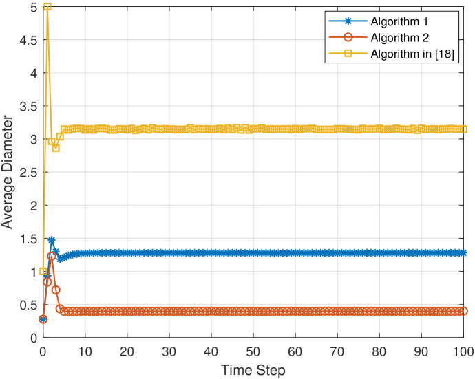
Figure 2: Comparison of Algorithm 1, Algorithm 2, and the algorithm in [18]. The diameter of each algorithm is averaged over $10000$ simulation runs. The averaged execution times in each time step for Algorithm 1, Algorithm 2, and the algorithm in [18] are $1.144\times 10^{-5}$s, $3.181\times 10^{-3}$s and $1.194\times 10^{-5}$s, respectively, where the simulation is conducted by using Matlab 2019b on a laptop with Intel Core i7-7700HQ@2.80GHz CPU.

IV-B Linear System with Identical Process Noise

Consider the linear system described by

$$\mathbf{x}_{k+1} =\begin{bmatrix}1&1\\ 0&1\end{bmatrix}\mathbf{x}_{k}+\begin{bmatrix}0.5\\ 1\end{bmatrix}\mathbf{w},$$ (32)

$$\mathbf{y}_{k} =\begin{bmatrix}1&0\end{bmatrix}\mathbf{x}_{k}+\mathbf{v}_{k},$$ (33)

where $\llbracket\mathbf{x}_{0}\rrbracket=[-10,10]\times[-10,10]$, $\llbracket\mathbf{w}\rrbracket=[-1,1]$, and $\llbracket\mathbf{v}_{k}\rrbracket=[-1,1]$. $\forall k\in\mathbb{N}_{0}$, $\mathbf{x}_{0},\mathbf{w},\mathbf{v}_{0:k}$ are unrelated.

If we replace $\mathbf{w}$ with $\mathbf{w}_{k}$ and assume Assumption 1 holds, the classical SMFing is Corollary 1 with

$$A=\begin{bmatrix}1&1\\ 0&1\end{bmatrix},\quad B=\begin{bmatrix}0.5\\ 1\end{bmatrix},\quad C=\begin{bmatrix}1&0\end{bmatrix},\quad D=1.$$ (34)

We employ the Projection-Based (PB) method in [27] to give the estimate $\llbracket\mathbf{x}_{k}|y_{0:k}\rrbracket$ exactly, labeled as PB-SMF 1.

Now we design the optimal SMF using Remark 3, and the modified system with $\mathbf{z}_{k}=[\mathbf{x}_{k}^{\mathrm{T}},\mathbf{w}_{k}]^{\mathrm{T}}=[\mathbf{x}_{k}^{(1)},\mathbf{x}_{k}^{(2)},\mathbf{w}_{k}]^{\mathrm{T}}$ is

$$\mathbf{z}_{k+1} =\begin{bmatrix}1&1&0.5\\ 0&1&1\\ 0&0&1\end{bmatrix}\mathbf{z}_{k},$$ (35)

$$\mathbf{y}_{k} =\begin{bmatrix}1&0&0\end{bmatrix}\mathbf{z}_{k}+\mathbf{v}_{k},$$ (36)

which gives the optimal filter, labeled as PB-SMF 2, when Corollary 1 is applied. Similarly to Section IV-A, we denote $\llbracket\mathbf{x}_{k}^{*}|y_{0:k}\rrbracket$ as the optimal posterior range, which can be derived by the projection of $\llbracket\mathbf{z}_{k}|y_{0:k}\rrbracket$ to the $x^{(1)}x^{(2)}$-plane.

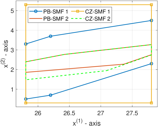
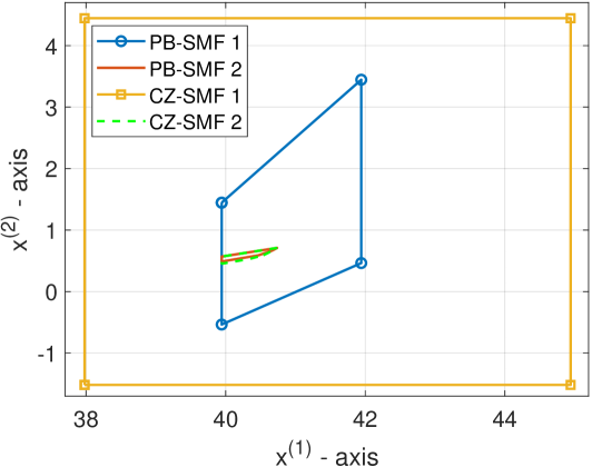
Figure 3: Comparisons of the PB-SMF and the CZ-SMF under the classical and the optimal SMFing frameworks at: (a) $k=10$, (b) $k=20$. CZ-SMF 1 (under the classical framework) and CZ-SMF 2 (under the optimal framework) are simulated with the help of CORA 2020 toolbox [28], where the degree-of-freedom order and the number of constraints are $0$ and $5$, respectively.

Fig. 3 shows the performance gap between the (optimal) PB-SMFs under the optimal and classical frameworks. We can see that $\llbracket\mathbf{x}_{10}^{*}|y_{0:10}\rrbracket$ (based on PB-SMF2) is smaller than $\llbracket\mathbf{x}_{10}|y_{0:10}\rrbracket$ (based on PB-SMF1) at $k=10$ in Fig. 3, and the area ratio is $27.1\%$; finally, $\llbracket\mathbf{x}_{10}^{*}|y_{0:20}\rrbracket$ becomes much smaller than $\llbracket\mathbf{x}_{20}|y_{0:20}\rrbracket$ at $k=20$ in Fig. 3, and the area ratio is $1.04\%$, which means approximately $99\%$ of the estimated range by the classical SMFing is excluded by the optimal SMFing. Besides, Fig. 3 also presents the gaps between the Constrained Zonotopic SMF (CZ-SMF) [22] under the optimal and classical frameworks. The area ratios are $19.0\%$ and $0.174\%$ for $k=10$ and $k=20$, respectively.

V Conclusion

In this work, we have studied the optimal SMFing problem for discrete-time systems. Based on the uncertain variables, we have put forward an optimal SMFing framework. Then, we have obtained the optimal SMF under non-stochastic Markov condition, and revealed the fundamental equivalence between the SMF and the Bayes filter. We have also shown that the classical SMF in the literature must rely on the non-stochastic Markov condition to guarantee optimality. When the Markovness is violated, the classical SMF is not optimal and can only provide an outer bound on the optimal estimation.

Appendix A Proof of Lemma 1

We only prove $\llbracket\mathbf{x}\rrbracket=\bigcup_{y\in\llbracket\mathbf{y}\rrbracket}\llbracket\mathbf{x}|y\rrbracket$, and the proof for $\llbracket\mathbf{y}\rrbracket=\bigcup_{x\in\llbracket\mathbf{x}\rrbracket}\llbracket\mathbf{y}|x\rrbracket$ is similar. From (3), we have $\bigcup_{y\in\llbracket\mathbf{y}\rrbracket}\llbracket\mathbf{x}|y\rrbracket=\bigcup_{y\in\llbracket\mathbf{y}\rrbracket}\left\{\mathbf{x}(\omega)\colon\omega\in\Omega_{\mathbf{y}=y}\right\}\stackrel{{\scriptstyle(a)}}{{=}}\left\{\mathbf{x}(\omega)\colon\omega\in\Omega\right\}=\llbracket\mathbf{x}\rrbracket$, where $(a)$ is from $\bigcup_{y\in\llbracket\mathbf{y}\rrbracket}\mathbf{x}(\Omega_{\mathbf{y}=y})=\mathbf{x}(\bigcup_{y\in\llbracket\mathbf{y}\rrbracket}\Omega_{\mathbf{y}=y})=\mathbf{x}(\Omega)$. Thus, (9) holds. $\blacksquare$

Appendix B Proof of Lemma 2

Firstly, we define $\llbracket\mathbf{x},y\rrbracket$ as $\{(\mathbf{x}(\omega),\mathbf{y}(\omega))\colon\mathbf{y}(\omega)=y,\omega\in\Omega\}=\{(\mathbf{x}(\omega),\mathbf{y}(\omega))\colon\omega\in\Omega_{\mathbf{y}=y}\}$. With (3), we have

$$\llbracket\mathbf{x},y\rrbracket=\llbracket\mathbf{x}|y\rrbracket\times\{y\},$$ (37)

and conversely we have

$$\llbracket\mathbf{x}|y\rrbracket=\operatorname*{Proj}_{(x,y)\mapsto x}\llbracket\mathbf{x},y\rrbracket,$$ (38)

where $\operatorname*{Proj}_{(x,y)\mapsto x}(\cdot)$ is a projection from the space w.r.t. $(x,y)$ to the subspace w.r.t. $x$ that $\operatorname*{Proj}_{(x,y)\mapsto x}(\mathcal{S}_{x},\mathcal{S}_{y})=\mathcal{S}_{x}$ for sets $\mathcal{S}_{x}$ and $\mathcal{S}_{y}$.

Secondly, we prove the following equation holds

$$\llbracket\mathbf{x},y\rrbracket=\llbracket\mathbf{x},\mathbf{y}\rrbracket\bigcap\left(\llbracket\mathbf{x}\rrbracket\times\{y\}\right).$$ (39)

With the RHS of the first equality in (4), the RHS of (39) can be rewritten as

$$\begin{split}&\Big{[}\bigcup_{y^{\prime}\in\llbracket\mathbf{y}\rrbracket}\big{(}\llbracket\mathbf{x}|y\rrbracket\times\{y^{\prime}\}\big{)}\Big{]}\bigcap\left(\llbracket\mathbf{x}\rrbracket\times\{y\}\right)\\ =&\bigcup_{y^{\prime}\in\llbracket\mathbf{y}\rrbracket}\left[\big{(}\llbracket\mathbf{x}|y^{\prime}\rrbracket\times\{y^{\prime}\}\big{)}\bigcap\left(\llbracket\mathbf{x}\rrbracket\times\{y\}\right)\right]\\ \stackrel{{\scriptstyle(a)}}{{=}}&\bigcup_{y\in\llbracket\mathbf{y}\rrbracket}\left[\big{(}\llbracket\mathbf{x}|y^{\prime}\rrbracket\bigcap\llbracket\mathbf{x}\rrbracket\big{)}\times\big{(}\{y^{\prime}\}\bigcap\{y\}\big{)}\right]\\ \stackrel{{\scriptstyle(b)}}{{=}}&\llbracket\mathbf{x}|y\rrbracket\times\{y\}\stackrel{{\scriptstyle(c)}}{{=}}\llbracket\mathbf{x},y\rrbracket,\end{split}$$ (40)

where $(a)$ follows $(\mathcal{S}_{1}\times\mathcal{S}_{2})\bigcap(\mathcal{S}_{3}\times\mathcal{S}_{4})=(\mathcal{S}_{1}\bigcap\mathcal{S}_{3})\times(\mathcal{S}_{2}\bigcap\mathcal{S}_{4})$ for sets $\mathcal{S}_{1},\ldots,\mathcal{S}_{4}$. Equality $(b)$ is established by (9) (which implies $\llbracket\mathbf{x}|y^{\prime}\rrbracket\subseteq\llbracket\mathbf{x}\rrbracket$) and $\mathcal{S}\times\emptyset=\emptyset$ for set $\mathcal{S}$. Then, $(c)$ follows from (37).

Thirdly, we prove a projection-based version of Bayes’ rule

$$\llbracket\mathbf{x}|y\rrbracket=\operatorname*{Proj}_{(x,y)\mapsto x}\Bigg{(}\bigcup_{x\in\llbracket\mathbf{x}\rrbracket}\bigg{[}\{x\}\times\left(\llbracket\mathbf{y}|x\rrbracket\bigcap\{y\}\right)\bigg{]}\Bigg{)}.$$ (41)

With (39) and the RHS of the second equality in (4), we get

$$\begin{split}\llbracket\mathbf{x},y\rrbracket&=\bigg{[}\bigcup_{x\in\llbracket\mathbf{x}\rrbracket}\big{(}\{x\}\times\llbracket\mathbf{y}|x\rrbracket\big{)}\bigg{]}\bigcap\left(\llbracket\mathbf{x}\rrbracket\times\{y\}\right)\\ &=\bigcup_{x\in\llbracket\mathbf{x}\rrbracket}\left[\big{(}\{x\}\times\llbracket\mathbf{y}|x\rrbracket\big{)}\bigcap\left(\llbracket\mathbf{x}\rrbracket\times\{y\}\right)\right]\\ &=\bigcup_{x\in\llbracket\mathbf{x}\rrbracket}\left[\big{(}\{x\}\bigcap\llbracket\mathbf{x}\rrbracket\big{)}\times\big{(}\llbracket\mathbf{y}|x\rrbracket\bigcap\{y\}\big{)}\right]\\ &=\bigcup_{x\in\llbracket\mathbf{x}\rrbracket}\left[\{x\}\times\big{(}\llbracket\mathbf{y}|x\rrbracket\bigcap\{y\}\big{)}\right].\end{split}$$ (42)

By (38) and (42), (41) is obtained.

Finally, we prove that (10) and (41) are equivalent. Let $\mathcal{T}_{1}$ and $\mathcal{T}_{2}$ denote the RHS of (41) and the RHS of (10), respectively. $\forall x^{\prime}\in\mathcal{T}_{1}$, we have $\llbracket\mathbf{y}|x^{\prime}\rrbracket\bigcap\{y\}\neq\emptyset$, since otherwise $\{x^{\prime}\}\times\big{(}\llbracket\mathbf{y}|x^{\prime}\rrbracket\bigcap\{y\}\big{)}=\emptyset$ which means $x^{\prime}\notin\mathcal{T}_{1}$. Observing that $x^{\prime}\in\llbracket\mathbf{x}\rrbracket$, we get $x^{\prime}\in\mathcal{T}_{2}$, and thus $\mathcal{T}_{1}\subseteq\mathcal{T}_{2}$. Conversely, $\forall x^{\prime\prime}\in\mathcal{T}_{2}$, we have $x^{\prime\prime}\in\llbracket\mathbf{x}\rrbracket$ and $\llbracket\mathbf{y}|x^{\prime\prime}\rrbracket\bigcap\{y\}\neq\emptyset$. Hence, $\{x^{\prime\prime}\}\times\big{(}\llbracket\mathbf{y}|x^{\prime\prime}\rrbracket\bigcap\{y\}\big{)}\neq\emptyset$ holds with $x^{\prime\prime}\in\llbracket\mathbf{x}\rrbracket$ which implies $x^{\prime\prime}\in\mathcal{T}_{1}$ and therefore $\mathcal{T}_{2}\subseteq\mathcal{T}_{1}$. Combining it with $\mathcal{T}_{1}\subseteq\mathcal{T}_{2}$, we get $\mathcal{T}_{1}=\mathcal{T}_{2}$. $\blacksquare$

Appendix C Proof of Theorem 1

We divide the proof of Theorem 1 into two parts, the prediction step and the update step.

For the prediction step, the law of total range in (9) gives

$$\llbracket\mathbf{x}_{k}|y_{0:k-1}\rrbracket=\bigcup_{x_{k-1}\in\llbracket\mathbf{x}_{k-1}|y_{0:k-1}\rrbracket}\llbracket\mathbf{x}_{k}|x_{k-1},y_{0:k-1}\rrbracket.$$ (43)

From (11), the following holds

$$\begin{split}\llbracket\mathbf{x}_{k}|x_{k-1},y_{0:k-1}\rrbracket&=\llbracket f(\mathbf{x}_{k-1},\mathbf{w}_{k-1})|x_{k-1},y_{0:k-1}\rrbracket\\ &=\llbracket f(x_{k-1},\mathbf{w}_{k-1})|x_{k-1},y_{0:k-1}\rrbracket\\ &\stackrel{{\scriptstyle(a)}}{{=}}f(x_{k-1},\llbracket\mathbf{w}_{k-1}|x_{k-1},y_{0:k-1}\rrbracket),\end{split}$$ (44)

where $(a)$ follows from (3) that

$$\begin{split}&\llbracket f(x_{k-1},\mathbf{w}_{k-1})|x_{k-1},y_{0:k-1}\rrbracket\\ =&\{f(x_{k-1},\mathbf{w}_{k-1}(\omega))\colon\omega\in\Omega_{\mathbf{x}_{k-1},\mathbf{y}_{0:k-1}=x_{k-1},y_{0:k-1}}\}\\ =&\{f(x_{k-1},w_{k-1})\colon w_{k-1}\in\llbracket\mathbf{w}_{k-1}|x_{k-1},y_{0:k-1}\rrbracket\}\\ =&f(x_{k-1},\llbracket\mathbf{w}_{k-1}|x_{k-1},y_{0:k-1}\rrbracket).\end{split}$$ (45)

Combining (43) with (44), we get (13).

For the update step, we prove it with Bayes’ rule for uncertain variables. From (10), we have

$$\llbracket\mathbf{x}_{k}|y_{0:k}\rrbracket\!=\!\Big{\{}x_{k}\!\in\llbracket\mathbf{x}_{k}|y_{0:k-1}\rrbracket\colon\llbracket\mathbf{y}_{k}|x_{k},y_{0:k-1}\rrbracket\bigcap\{y_{k}\}\neq\emptyset\Big{\}}.$$ (46)

Similarly to dealing with $\llbracket\mathbf{x}_{k}|x_{k-1},y_{0:k-1}\rrbracket$ in (44), we have $\llbracket\mathbf{y}_{k}|x_{k},y_{0:k-1}\rrbracket=g_{k}(x_{k},\llbracket\mathbf{v}_{k}|x_{k},y_{0:k-1}\rrbracket)$. Thus, the RHS of (46) can be rewritten as (14).

By Definition 1, the set of all possible $x_{k}$ given $y_{0:k}$ is exact the posterior range $\llbracket\mathbf{x}_{k}|y_{0:k}\rrbracket$. Therefore, $X_{k}^{*}(y_{0:k})=\llbracket\mathbf{x}_{k}|y_{0:k}\rrbracket$ which satisfies the condition $X_{k}^{*}(y_{0:k})\subseteq X^{\prime}_{k}(y_{0:k})$ holds for any $X^{\prime}_{k}$ and $y_{0:k}$ in Definition 3. $\blacksquare$

Appendix D Proof of Theorem 2

Before start, we need the following two lemmas.

Lemma 3 (Function of Conditional Range).

Given uncertain variables $\mathbf{u}_{1},\mathbf{u}_{2}$ and map $h$, $\llbracket h(\mathbf{u}_{1})|u_{2}\rrbracket=h(\llbracket\mathbf{u}_{1}|u_{2}\rrbracket)$ holds.

Proof:

$\llbracket h(\mathbf{u}_{1})|u_{2}\rrbracket=\{h(\mathbf{u}_{1}(\omega))\colon\omega\in\Omega_{\mathbf{u}_{2}=u_{2}}\}=h(\{\mathbf{u}_{1}(\omega)\colon\omega\in\Omega_{\mathbf{u}_{2}=u_{2}}\})=h(\llbracket\mathbf{u}_{1}|u_{2}\rrbracket)$. ∎

Lemma 4 (Invariance of Unrelatedness under Maps).

If $\mathbf{u}_{1}$ and $\mathbf{u}_{2}$ are unrelated, $h_{1}(\mathbf{u}_{1})$ and $h_{2}(\mathbf{u}_{2})$ are unrelated, i.e.,

$$\llbracket h_{1}(\mathbf{u}_{1})|h_{2}(u_{2})\rrbracket=\llbracket h_{1}(\mathbf{u}_{1})\rrbracket,\quad\forall u_{2}\in\llbracket\mathbf{u}_{2}\rrbracket.$$ (47)

Proof:

By Lemma 3, the LHS and RHS of equation (47) can be written as $h_{1}(\llbracket\mathbf{u}_{1}|h_{2}(u_{2})\rrbracket)$ and $h_{1}(\llbracket\mathbf{u}_{1}\rrbracket)$, respectively. Since a sufficient condition to $h_{1}(\llbracket\mathbf{u}_{1}|h_{2}(u_{2})\rrbracket)=h_{1}(\llbracket\mathbf{u}_{1}\rrbracket)$ is

$$\llbracket\mathbf{u}_{1}|h_{2}(u_{2})\rrbracket=\llbracket\mathbf{u}_{1}\rrbracket,$$ (48)

we need to prove that (48) holds for $u_{2}\in\llbracket\mathbf{u}_{2}\rrbracket$.

$\forall u_{2}\in\llbracket\mathbf{u}_{2}\rrbracket$, we have $\llbracket\mathbf{u}_{1}|u_{2}\rrbracket=\{\mathbf{u}_{1}(\omega)\colon\omega\in\Omega_{\mathbf{u}_{2}=u_{2}}\}$ and $\llbracket\mathbf{u}_{1}|h_{2}(u_{2})\rrbracket=\{\mathbf{u}_{1}(\omega)\colon\omega\in\Omega_{h_{2}(\mathbf{u}_{2})=h_{2}(u_{2})}\}$. As $\Omega_{h_{2}(\mathbf{u}_{2})=h_{2}(u_{2})}=\mathbf{u}_{2}^{-1}\circ h_{2}^{-1}(\{h_{2}(u_{2})\})$ and $h_{2}^{-1}(\{h_{2}(u_{2})\})\supseteq\{u_{2}\}$, we get $\Omega_{h_{2}(\mathbf{u}_{2})=h_{2}(u_{2})}\supseteq\Omega_{\mathbf{u}_{2}=u_{2}}$ which implies $\llbracket\mathbf{u}_{1}|h_{2}(u_{2})\rrbracket\supseteq\llbracket\mathbf{u}_{1}|u_{2}\rrbracket$. Thus (48) is established by

$$\llbracket\mathbf{u}_{1}\rrbracket\supseteq\llbracket\mathbf{u}_{1}|h_{2}(u_{2})\rrbracket\supseteq\llbracket\mathbf{u}_{1}|u_{2}\rrbracket\stackrel{{\scriptstyle(a)}}{{=}}\llbracket\mathbf{u}_{1}\rrbracket,$$ (49)

where $(a)$ follows from the fact that $\forall u_{2}\in\llbracket\mathbf{u}_{2}\rrbracket$, $\llbracket\mathbf{u}_{1}|u_{2}\rrbracket=\llbracket\mathbf{u}_{1}\rrbracket$ for unrelated $\mathbf{u}_{1}$ and $\mathbf{u}_{2}$ [see (7)]. Therefore, (47) holds, and combining it with (7), we know that $h_{1}(\mathbf{u}_{1})$ and $h_{2}(\mathbf{u}_{2})$ are also unrelated. ∎

Now we prove the prediction and update steps in Theorem 2, respectively. In the prediction step, for $\llbracket\mathbf{w}_{k-1}|x_{k-1},y_{0:k-1}\rrbracket$ in (13), we know that the collection of $\mathbf{x}_{k-1},\mathbf{y}_{0:k-1}$ is a function of $\mathbf{w}_{0:k-2},\mathbf{v}_{0:k-1},\mathbf{x}_{0}=:{\boldsymbol{\varpi}}_{k-1}$, i.e., $(\mathbf{x}_{k-1},\mathbf{y}_{0:k-1})=:\xi({\boldsymbol{\varpi}}_{k-1})$. By Assumption 1, $\mathbf{w}_{k-1}$ and ${\boldsymbol{\varpi}}_{k-1}$ are unrelated. Thus, applying Lemma 4, we get

$$\llbracket\mathbf{w}_{k-1}|x_{k-1},y_{0:k-1}\rrbracket=\llbracket\mathbf{w}_{k-1}|\xi(\varpi_{k-1})\rrbracket=\llbracket\mathbf{w}_{k-1}\rrbracket,$$ (50)

where $\varpi_{k-1}$ is the realization of ${\boldsymbol{\varpi}}_{k-1}$. With (50), (13) becomes (15).

In the update step, we can use a similar technique in (50) to obtain $\llbracket\mathbf{v}_{k}|x_{k},y_{0:k-1}\rrbracket=\llbracket\mathbf{v}_{k}\rrbracket$. Then, (14) becomes

$$\begin{split}&\!\!\!\!\left\{x_{k}\in\llbracket\mathbf{x}_{k}|y_{0:k-1}\rrbracket\colon g_{k}(x_{k},\llbracket\mathbf{v}_{k}\rrbracket)\bigcap\{y_{k}\}\neq\emptyset\right\}\\ &\!\!\!\!\stackrel{{\scriptstyle(a)}}{{=}}\!\!\bigcup_{v_{k}\in\llbracket\mathbf{v}_{k}\rrbracket}\left\{x_{k}\in\llbracket\mathbf{x}_{k}|y_{0:k-1}\rrbracket\colon\{x_{k}\}=g_{k,v_{k}}^{-1}(\{y_{k}\})\right\}\\ &\!\!\!\!=\!\!\bigcup_{v_{k}\in\llbracket\mathbf{v}_{k}\rrbracket}\left[g_{k,v_{k}}^{-1}(\{y_{k}\})\bigcap\llbracket\mathbf{x}_{k}|y_{0:k-1}\rrbracket\right]=\mathrm{RHS~{}of~{}\eqref{eqn:Update - Optimal Set-Membership Filter}}.\end{split}$$ (51)

where $(a)$ is from $g_{k}(x_{k},\llbracket\mathbf{v}_{k}\rrbracket)=\bigcup_{v_{k}\in\llbracket\mathbf{v}_{k}\rrbracket}\{g_{k}(x_{k},v_{k})\}$ and the fact that $\{g_{k}(x_{k},v_{k})\}\bigcap\{y_{k}\}\neq\emptyset$ iff $\{x_{k}\}=g_{k,v_{k}}^{-1}(\{y_{k}\})$, in which $g_{k,v_{k}}^{-1}(\{y_{k}\})=\{x_{k}\colon g_{k}(x_{k},v_{k})=y_{k}\}$. $\blacksquare$

Appendix E Proof of Theorem 3

In the initialization step, $\llbracket\mathbf{x}_{0}^{*}\rrbracket=\llbracket\mathbf{x}_{0}\rrbracket$ holds. In the update step at $k=0$, since (9) implies $\llbracket\mathbf{x}|y\rrbracket\subseteq\llbracket\mathbf{x}\rrbracket$, we have $\llbracket\mathbf{v}_{0}|x_{0}\rrbracket\subseteq\llbracket\mathbf{v}_{0}\rrbracket$ in (14). Thus,

$$\llbracket\mathbf{x}_{0}^{*}|y_{0}\rrbracket=\left\{x_{0}\!\in\!\llbracket\mathbf{x}_{0}^{*}\rrbracket\colon g_{0}(x_{0},\llbracket\mathbf{v}_{0}|x_{0}\rrbracket)\bigcap\{y_{0}\}\neq\emptyset\right\}\\ \subseteq\left\{x_{0}\!\in\!\llbracket\mathbf{x}_{0}^{*}\rrbracket\colon g_{0}(x_{0},\llbracket\mathbf{v}_{0}\rrbracket)\bigcap\{y_{0}\}\neq\emptyset\right\}\stackrel{{\scriptstyle(a)}}{{=}}\llbracket\mathbf{x}_{0}|y_{0}\rrbracket,$$ (52)

where $(a)$ follows from (16) and (51). Similarly, in the prediction step at $k=1$, we have $\llbracket\mathbf{w}_{1}|x_{0},y_{0}\rrbracket\subseteq\llbracket\mathbf{w}_{1}\rrbracket$, which implies $\llbracket\mathbf{x}_{1}^{*}|y_{0}\rrbracket\subseteq\llbracket\mathbf{x}_{1}|y_{0}\rrbracket$. Proceeding forward, we get $\llbracket\mathbf{x}_{k}^{*}|y_{0:k}\rrbracket\subseteq\llbracket\mathbf{x}_{k}|y_{0:k}\rrbracket$ for $k\in\mathbb{N}_{0}$. $\blacksquare$

References

• [1] S. Särkkä, Bayesian filtering and smoothing.   New York, NY, USA: Cambridge University Press, 2013.
• [2] Z. Chen, “Bayesian filtering: From kalman filters to particle filters, and beyond,” Statistics, vol. 182, no. 1, pp. 1–69, 2003.
• [3] A. H. Jazwinski, Stochastic Processes and Filtering Theory.   New York, NY, USA: New York, USA: Academic Press, 1970.
• [4] R. E. Kalman, “A new approach to linear filtering and prediction problems,” J. Basic Eng., vol. 82, no. 1, pp. 35–45, Mar. 1960.
• [5] H. S. Witsenhausen, “Minimax controls of uncertain systems,” M.I.T. Electron. Syst. Lab., Cambridge, Tech. Rep. Mass. Rept. ESL-R-269 (NASA Rept. N66-33441), May 1966.
• [6] H. Witsenhausen, “Sets of possible states of linear systems given perturbed observations,” IEEE Trans. Autom. Control, vol. 13, no. 5, pp. 556–558, Oct. 1968.
• [7] L. Jaulin, M. Kieffer, O. Didrit, and E. Walter, Applied Interval Analysis.   London, UK: Springer-Verlag, 2001.
• [8] D. Efimov, T. Raïssi, S. Chebotarev, and A. Zolghadri, “Interval state observer for nonlinear time varying systems,” Automatica, vol. 49, no. 1, pp. 200–205, Jan. 2013.
• [9] W. Tang, Z. Wang, Y. Wang, T. Raïssi, and Y. Shen, “Interval estimation methods for discrete-time linear time-invariant systems,” IEEE Trans. Autom. Control, vol. 64, no. 11, pp. 4717–4724, Nov. 2019.
• [10] F. Schweppe, “Recursive state estimation: Unknown but bounded errors and system inputs,” IEEE Trans. Autom. Control, vol. 13, no. 1, pp. 22–28, Feb. 1968.
• [11] D. Bertsekas and I. Rhodes, “Recursive state estimation for a set-membership description of uncertainty,” IEEE Trans. Autom. Control, vol. 16, no. 2, pp. 117–128, Apr. 1971.
• [12] F. L. Chernousko, “Optimal guaranteed estimates of indeterminacies with the aid of ellipsoids. parts I-III,” Eng. Cybern., vol. 18, pp. 1–9, 1980.
• [13] E. Fogel and Y. Huang, “On the value of information in system identification—bounded noise case,” Automatica, vol. 18, no. 2, pp. 229–238, Mar. 1982.
• [14] D. G. Maksarov and J. P. Norton, “State bounding with ellipsoidal set description of the uncertainty,” Int. J. Control, vol. 65, no. 5, pp. 847–866, Jan. 1996.
• [15] C. Durieu, É. Walter, and B. Polyak, “Multi-input multi-output ellipsoidal state bounding,” J. Optimization Theory and Appl., vol. 111, no. 2, pp. 273–303, Nov. 2001.
• [16] L. Chisci, A. Garulli, and G. Zappa, “Recursive state bounding by parallelotopes,” Automatica, vol. 32, no. 7, pp. 1049–1055, Jul. 1996.
• [17] C. Combastel, “A state bounding observer based on zonotopes,” in Proc. Eur. Control Conf. (ECC), Sep. 2003, pp. 2589–2594.
• [18] T. Alamo, J. Bravo, and E. Camacho, “Guaranteed state estimation by zonotopes,” Automatica, vol. 41, no. 6, pp. 1035–1043, Jun. 2005.
• [19] T. Alamo, J. Bravo, M. Redondo, and E. Camacho, “A set-membership state estimation algorithm based on dc programming,” Automatica, vol. 44, no. 1, pp. 216–224, Jan. 2008.
• [20] V. T. H. Le, C. Stoica, T. Alamo, E. F. Camacho, and D. Dumur, “Zonotopic guaranteed state estimation for uncertain systems,” Automatica, vol. 49, no. 11, pp. 3418–3424, Nov. 2013.
• [21] C. Combastel, “Zonotopes and kalman observers: Gain optimality under distinct uncertainty paradigms and robust convergence,” Automatica, vol. 55, pp. 265–273, May 2015.
• [22] J. K. Scott, D. M. Raimondo, G. R. Marseglia, and R. D. Braatz, “Constrained zonotopes: A new tool for set-based estimation and fault detection,” Automatica, vol. 69, pp. 126–136, Jul. 2016.
• [23] B. S. Rego, D. M. Raimondo, and G. V. Raffo, “Set-based state estimation of nonlinear systems using constrained zonotopes and interval arithmetic,” in Proc. Eur. Control Conf. (ECC), Jun. 2018, pp. 1584–1589.
• [24] B. S. Rego, G. V. Raffo, J. K. Scott, and D. M. Raimondo, “Guaranteed methods based on constrained zonotopes for set-valued state estimation of nonlinear discrete-time systems,” Automatica, vol. 111, p. 108614, Jan. 2020.
• [25] G. N. Nair, “A nonstochastic information theory for communication and state estimation,” IEEE Trans. Autom. Control, vol. 58, no. 6, pp. 1497–1510, Jun. 2013.
• [26] P. H. Leong and G. N. Nair, “Set-membership filtering using random samples,” in Proc. Int. Conf. Inform. Fusion (FUSION), July 2016, pp. 1087–1094.
• [27] J. S. Shamma and K.-Y. Tu, “Set-valued observers and optimal disturbance rejection,” IEEE Trans. Autom. Control, vol. 44, no. 2, pp. 253–264, Feb. 1999.
• [28] M. Althoff, N. Kochdumper, and M. Wetzlinger, “CORA 2020 manual,” 2020. [Online]. Available: https://tumcps.github.io/CORA/