A Mathematical Assessment of the Isolation Random
Forest Method for Anomaly Detection in Big Data

Abstract

We present the mathematical analysis of the Isolation Random Forest Method (IRF Method) for anomaly detection, introduced in [1] and [2]. We prove that the IRF space can be endowed with a probability induced by the Isolation Tree algorithm (iTree). In this setting, the convergence of the IRF method is proved, using the Law of Large Numbers. A couple of counterexamples are presented to show that the method is inconclusive and no certificate of quality can be given, when using it as a means to detect anomalies. Hence, an alternative version of the method is proposed whose mathematical foundation is fully justified. Furthermore, a criterion for choosing the number of sampled trees needed to guarantee confidence intervals of the numerical results is presented. Finally, numerical experiments are presented to compare the performance of the classic method with the proposed one.

1 Introduction

Anomaly detection in big data is an important field of research due to its applications, the presence of anomalies may indicate disease of individuals, fraudulent transactions and network security breaches, among others. There is a remarkable number of methods for anomaly detection following different paradigms, some of these are distance-based (see [3, 4, 5]), classification-based (see [6, 7]), cluster-based (see [8]), density-based (see [9], [10]) and isolation-based (see [1, 2, 11, 12]). In general, it is not possible to compare these methods from a unified point of view, because many of them were developed for particular types problems with data sets satisfying specific hypotheses, although some techniques are applicable to a broader class of problems, see [13] and [14] for comprehensive surveys on the field.

In the present work we focus on the mathematical analysis of the Isolation Random Forest Method, from now on, denoted by IRF. Despite the popularity of the IRF method, to the authors’ best knowledge, it has not been analyzed mathematically. For instance, there is no rigorous proof that the method converges, there is no analysis about the number of iterations needed to guarantee confidence intervals for the computed values. Some scenarios where the method performs poorly have been pointed out in [1] and [2], but there are no general recommendations/guidelines for a setting where the IRF Method runs successfully. In the present work, all these aspects are addressed with mathematical rigor.

Due to its popularity, the IRF method has been analyzed from the empirical point of view and some of its deficiencies, detected experimentally, have been addressed and an enhanced with good results, from the empirical point of view. Following the Machine Learning modern point of view, most of these attempts, consider that one or more samples must be taken from the available data as a training set. The ultimate goal of such training is to build a probabilistic distribution locating the outliers according to a probabilistic distribution on the $\bm{\mathbbm{R}}^{d}$ region the data containing the data; once the distribution is deduced the non-used data serve as testing instances. Some of the IRF method’s aforementioned weaknesses were that it failed to detect clustered outliers (see [15]) and that for certain particular data configurations some ghost sub-regions in the probability distribution show up (see [16]). In both works the authors coincide in modifying the data split criterion in which the isolation trees are constructed, as a way to amend the method’s flaws. To that end, in [15] the authors propose a separation hyperplane for data splitting, which is computed using an empirical optimization process executed on a set of random oblique hyperplanes generated in every iteration of the algorithm presented algorithm (SciForest: Isolation Forest with Split-selection Criterion), the idea is similar to that in [17]. This way, the randomness is preserved, while refined through a deterministic method of optimization. In the reference [16], the authors tackle the original IRF method’s limitations with two approaches. In both cases the aim is to use random oblique hyerplanes instead of exclusively using axis-parallel hypeplanes as in the original method; unlike [15], no optimization process is applied. Both works report that the novelty proposed methods outperform the original one. However, their results are established empirically in the same way that the flaws of the original IRF method were detected. Essentially, the mainstream is to keep enhancing the original method using experimental validation. We differ radically from this approach as we seek to understand the method through mathematical arguments of theoretical nature; later we use experiments to illustrate our results.

The paper is organized as follows, in the introductory section the notation and general setting are presented; the IRF Method is reviewed for the sake of completeness and a proof is given that the iTree algorithm is well-defined. Section 2 presents the analysis of the method in the general setting: the underlying probabilistic structure is stated, the convergence of the method is established, the cardinality of the isolation random forest (IRF) is presented and two examples are given to analytically prove the inconclusiveness of the IRF Method in its original form. In Section 3, IRF is analyzed for the 1D case and proved to be a suitable tool for anomaly detection in this particular setting. This is done recalling a closely related algorithm, next, estimates for the values of the expected height and variance are given; the section closes introducing an alternative version of method (the Direction Isolation Random Forest Method, DIRF) whose mathematical foundation is fully justified. Finally, Section 4 presents numerical examples examining the performance of both methods IRF and DIRF.

Remark 1 (A note about the paper’s organization).

The Authors realize that the organization of the paper may rise some questions and disagreements, as it first visits the multidimensional case $\bm{\mathbbm{R}}^{d}$ (Section 2) and then analyzes the 1D case (Section 3). At first sight it may seem natural to exchange the order of these sections due to the level of generality they expose. The Authors did this exercise (privately) and concluded that such exposition would enlighten new features, but obscure some aspects they consider as priority in this work. The actual choice was made pursuing a balance between brevity, clarity and avoiding redundancy in the exposition. However, for a reader more interested in the mathematical techniques, than the analysis of the algorithms, it may be more beneficial to read first section 3 and then section 2.

1.1 Preliminaries

In this section the general setting and preliminaries of the problem are presented. We start introducing the mathematical notation. For any natural number $N\in\bm{\mathbbm{N}}$, the symbol $[N]\overset{\mathbf{def}}{=}\{1,2,\ldots,N\}$ indicates the set/window of the first $N$ natural numbers. For any set $E$ we denote by $\#E$, $\wp(E)$ its cardinal and power set respectively. For any interval $I\subseteq\bm{\mathbbm{R}}$ we denote by $|I|$ its length. Random variables will be represented with upright capital letters, namely $\mathsf{X},\mathsf{Y},\mathsf{Z}$ and its respective expectations with $\bm{\mathbb{E}}(\mathsf{X}),\bm{\mathbb{E}}(\mathsf{Y}),\bm{\mathbb{E}}(\mathsf{Z})$. Vectors are indicated with bold letters, namely $\mathbf{p},\mathbf{q},\mathbf{r}...$, etc. The canonical basis in $\bm{\mathbbm{R}}^{d}$ is written $\{\widehat{\mathbf{e}}_{1},\ldots,\widehat{\mathbf{e}}_{d}\}$, the projections from $\bm{\mathbbm{R}}^{d}$ onto the $j$-th coordinate are denoted by $\pi_{j}(\mathbf{x})\overset{\mathbf{def}}{=}\mathbf{x}\cdot\widehat{\mathbf{e}}_{j}$ for all $j\in[d]$, where $\mathbf{x}\in\bm{\mathbbm{R}}^{d}$.

The isolation random tree algorithm (iTree) for a set of points in $\bm{\mathbbm{R}}^{d}$ is defined recursively as follows

Definition 1 (The iTree Algorithm, introduced in [1, 2]).

Let $S\overset{\mathbf{def}}{=}\{\mathbf{x}_{0},\mathbf{x}_{1},\ldots,\mathbf{x}_{N}\}$ be a set of points in $\bm{\mathbbm{R}}^{d}$.

1. An isolation random tree $T$ (iTree), associated to this set is defined recursively as follows:

   1. Define the tree root as $\operatorname*{rt}(T)\overset{\mathbf{def}}{=}S$.

   2. Define the sets

      $$\pi_{j}(S)\overset{\mathbf{def}}{=}\{\pi_{j}(\mathbf{x}):\mathbf{x}\in S\}, 1\leq j\leq d, \Omega_{C}\overset{\mathbf{def}}{=}\{j\in[d]:\#\pi_{j}(S)\geq 2\}.$$ (1)

   3. If the set $S$ has two or more points (equivalently, if $\Omega_{C}\neq\emptyset$), choose randomly $j$ in $\Omega_{C}$ and next choose randomly $p\in(\min\pi_{j}(S),\max\pi_{j}(S))$ (the split value).

   4. Perform an isolation random tree on the left set of data $S_{\mathop{}\!\mathrm{left}}\overset{\mathbf{def}}{=}\{\mathbf{x}\in S:\mathbf{x}\cdot\widehat{\mathbf{e}}_{j}<p\}$, denoted by $T_{\mathop{}\!\mathrm{left}}$. Next, include the arc $\big{(}\operatorname*{rt}(T),\operatorname*{rt}(T_{\mathop{}\!\mathrm{left}})\big{)}$ in the edges of the tree $E(T)$; where $\operatorname*{rt}(T_{\mathop{}\!\mathrm{left}})=S_{\mathop{}\!\mathrm{left}}$ indicates the root of $T_{\mathop{}\!\mathrm{left}}$.

   5. Perform an isolation random tree on the right set of data $S_{\mathop{}\!\mathrm{right}}\overset{\mathbf{def}}{=}\{\mathbf{x}\in S:\mathbf{x}\cdot\widehat{\mathbf{e}}_{j}\geq p\}$, denoted by $T_{\mathop{}\!\mathrm{right}}$. Next, define the arc $\big{(}\operatorname*{rt}(T),\operatorname*{rt}(T_{\mathop{}\!\mathrm{right}})\big{)}$ in the edges of the tree $E(T)$, where $\operatorname*{rt}(T_{\mathop{}\!\mathrm{right}})=S_{\mathop{}\!\mathrm{right}}$ indicates the root of $T_{\mathop{}\!\mathrm{right}}$.

2. We denote the set of all possible isolation random trees associated to the set $S$ by $\operatorname*{\Omega_{IRF}}(S)$, whenever the context is clear, we simply write $\operatorname*{\Omega_{IRF}}$ and we refer to it as the isolation random forest.

For the sake of completeness we present the iTree Algorithm’s pseudocode in 1.

Algorithm 1 Isolation Random Tree (introduced in [1, 2]), returns a rooted tree with $N$ vertices. The vertices are subsets of the input data set $S=\big{\{}\mathbf{x}_{n}:n\in[N]\big{\}}\subseteq\bm{\mathbbm{R}}^{d}$.

1:procedure Isolation Random Tree(Data Set $S=\big{\{}\mathbf{x}_{n}:n\in[N]\big{\}}$.)

2:     $\text{VBT}=\emptyset$ $\triangleright$ Initializing the Vertex set in the Binary Tree as empty

3:     $\text{ABT}=\emptyset$ $\triangleright$ Initializing the list of Arcs in the Binary Tree as empty

4:     $\operatorname*{rt}=S$ $\triangleright$ Initializing the root as empty

5:     $S\rightarrow\text{VBT}$ $\triangleright$ Push the set $S$ to VBT

6:     function Branch($S,\text{VBT},\text{ABT},\operatorname*{rt}$)

7:         if $\#\Omega_{C}=1$  then $\triangleright$ Checking when to stop

8:              return $\text{VBT},\text{ABT}$

9:         else

10:              choose $j\in\Omega_{C}$ randomly $\triangleright$ Choosing the split direction.

11:              define $\pi_{j}(S)\overset{\mathbf{def}}{=}\big{\{}\pi_{j}(\mathbf{x}):\mathbf{x}\in S\big{\}}$, $\triangleright$ Data set projected onto the $j$-th direction

12:              choose $p\in\big{(}\min\pi_{j}(S),\max\pi_{j}(S)\big{)}$ randomly $\triangleright$ Choosing the split value.

13:              define $S_{\mathop{}\!\mathrm{left}}\overset{\mathbf{def}}{=}\big{\{}\mathbf{x}\in S:\mathbf{x}\cdot\widehat{\mathbf{e}}_{j}<p\big{\}}$, $S_{\mathop{}\!\mathrm{right}}\overset{\mathbf{def}}{=}\big{\{}\mathbf{x}\in S:\mathbf{x}\cdot\widehat{\mathbf{e}}_{j}\geq p\big{\}}$ $\triangleright$ Left and Right subsets

14:              $S_{\mathop{}\!\mathrm{left}}\rightarrow\text{VBT}$, $(\operatorname*{rt},S_{\mathop{}\!\mathrm{left}})\rightarrow\text{ABT}$ $\triangleright$ Push the set $S_{\mathop{}\!\mathrm{left}}$ to VBT and arc $(\operatorname*{rt},S_{\mathop{}\!\mathrm{left}})$ to ABT

15:              Branch$\big{(}S_{\mathop{}\!\mathrm{left}},\text{VBT},\text{ABT},\operatorname*{rt}\big{)}$

16:              $S_{\mathop{}\!\mathrm{right}}\rightarrow\text{VBT}$, $(\operatorname*{rt},S_{\mathop{}\!\mathrm{right}})\rightarrow\text{ABT}$ $\triangleright$ Push the set $S_{\mathop{}\!\mathrm{right}}$ to VBT and arc $(\operatorname*{rt},S_{\mathop{}\!\mathrm{right}})$ to ABT

17:              Branch$\big{(}S_{\mathop{}\!\mathrm{right}},\text{VBT},\text{ABT},\operatorname*{rt}\big{)}$

18:         end if

19:     end function

20:end procedure

Proposition 1.

Given an arbitrary set $S\overset{\mathbf{def}}{=}\{\mathbf{x}_{0},\mathbf{x}_{1},\ldots,\mathbf{x}_{N}\}$ in $\bm{\mathbbm{R}}^{d}$, the iTree algorithm described in Definition 1 needs $N$ instances to isolate every point in $S$.

Proof.

We proceed by induction on the number of data $N$. For $N=1$ the result is trivial.

Assume now that the result holds true for $k\leq N-1$ and let $S\overset{\mathbf{def}}{=}\{\mathbf{x}_{0},\mathbf{x}_{1},\ldots,\mathbf{x}_{N}\}$ be arbitrary in $\bm{\mathbbm{R}}^{d}$. Since $\#S\geq 2$, the set $\Omega_{C}$ (defined in (1)) must be nonempty. Choose randomly an index $j$ in $\Omega_{C}$ and choose randomly $p\in(\min S_{j},\max S_{j})$. Thus, after one instance of the algorithm the left and right subsets are defined and they satisfy

$$\#S_{\mathop{}\!\mathrm{left}}<N, \#S_{\mathop{}\!\mathrm{right}}<N, \#S_{\mathop{}\!\mathrm{left}}+\#S_{\mathop{}\!\mathrm{right}}=N.$$

Then, applying the induction hypothesis on each, the left and right subsets, it follows that the total of needed instances is

$$1+(\#S_{\mathop{}\!\mathrm{left}}-1)+(\#S_{\mathop{}\!\mathrm{right}}-1)=\#S_{\mathop{}\!\mathrm{left}}+\#S_{\mathop{}\!\mathrm{right}}-1=N-1,$$

which completes the proof. ∎

Definition 2 (The IRF Method, introduced in [1, 2]).

Given an input data set $S\overset{\mathbf{def}}{=}\{\mathbf{x}_{1},\ldots,\mathbf{x}_{N}\}\subseteq\bm{\mathbbm{R}}^{d}$, a number of Bernoulli trials $K$ and an anomaly threshold criterion.

1. For each Bernoulli trial $k=1,\ldots,K$, perform iTree on $S$ (see Defintion 1 and/or Algorithm 1) and store the heights $\{h_{k}(\mathbf{x}):\mathbf{x}\in S\}$ in a Log.

2. For each $\mathbf{x}\in S$, define $\mathsf{H}_{\text{IRF}}(\mathbf{x})$ as the average height of the collection of heights $\{h_{k}(\mathbf{x}):k=1,\ldots,K\}$.

3. Declare as anomalies $A\overset{\mathbf{def}}{=}\{\mathbf{x}\in S:\mathsf{H}_{\text{IRF}}(\mathbf{x})\text{ satisfies the anomaly threshold criterion}\}$.

Observe that due to Proposition 1 the iTree Algorithm and consequently the IRF method are well-defined. For brevity, we postpone until Theorem 2 in Section 2, the proof showing that the isolation random forest can be endowed with a probability measure, defined by the iTree algorithm.

2 The General Setting

This section presents the features of the isolation random forest that can be proved in general, these are: its probability structure, its cardinality and the fact that the IRF method converges and is well-defined. For the analysis of the general setting first we need to introduce a hypothesis

Hypothesis 1.

Given a set of data $S=\{\mathbf{x}_{0},\ldots,\mathbf{x}_{N}\}\subseteq\bm{\mathbbm{R}}^{d}$, from now on it will be assumed that no coordinates are repeated i.e.

$$\#\pi_{j}(S)=N+1, \text{for all }j=1,\ldots,d.$$ (2)

Here $\pi_{j}(S)$ is the $j$-th projection of the set $S$ as defined in Equation (1).

Definition 3.

Let $S=\{\mathbf{x}_{0},\ldots,\mathbf{x}_{N}\}\subseteq\bm{\mathbbm{R}}^{d}$ be a data set satisfying Hypothesis 1.

1. For each $j\in[d]$ denote by $\mathcal{P}^{(j)}\overset{\mathbf{def}}{=}\big{\{}I^{(j)}_{n}:n\in[N]\big{\}}$, the family of intervals defined by sorting the points of the set $\pi_{j}(S)=\big{\{}\mathbf{x}_{n}\cdot\widehat{\mathbf{e}}_{j}:n=0,\ldots,N\big{\}}$.

2. Define the grid of the set by $G_{S}\overset{\mathbf{def}}{=}\prod\limits_{j\,=\,1}^{d}\pi_{j}(S)$.

(See Figure 1 (a) for an illustration when $S\subseteq\bm{\mathbbm{R}}^{2}$.)

(a) Grid $G_{S}$, $S\subseteq\bm{\mathbbm{R}}^{2}$ satisfies Hypothesis 2. A potential ancestor is delimited in thick line

(b) Two possible alternatives (marked with $\blacksquare$ and $\blacklozenge$) generating the potential ancestor drawn in the figure of the left.

Figure 1: The figure (a) depicts the grid $G_{S}=\big{\{}0,p_{1},\ldots,p_{N}\big{\}}\times\big{\{}0,q_{1},\ldots,q_{N}\big{\}}=\{\mathbf{x}\cdot\widehat{\mathbf{e}}_{1}:\mathbf{x}\in S\}\times\{\mathbf{x}\cdot\widehat{\mathbf{e}}_{2}:\mathbf{x}\in S\}$, of a particular set $S$ satisfying Hypothesis 2. The corner $p_{k}\widehat{\mathbf{e}}_{1}+q_{\ell}\widehat{\mathbf{e}}_{2}$ defines a potential ancestor, however it may or may not belong to $S$. The figure (b) displays two possible ways to generate the potential ancestor of figure (a). First, when the point $p_{k}\widehat{\mathbf{e}}_{1}+q_{\ell}\widehat{\mathbf{e}}_{2}$, marked with $\blacksquare$ belongs to $S$. A second option occurs when the couple of points $p_{2}\widehat{\mathbf{e}}_{1}+q_{\ell}\widehat{\mathbf{e}}_{2}$, $p_{k}\widehat{\mathbf{e}}_{1}+q_{1}\widehat{\mathbf{e}}_{2}$, marked with $\blacklozenge$ belong to $S$. It is direct to see that there are $(k-1)\times(\ell-1)+1$ possibilities to generate the potential ancestor at hand, but at most one of them is present in a given configuration/set.

Remark 2.

Observe that Hypothesis 1 is mild because, it will be satisfied with probability one for any sample of $N+1$ elements from $\bm{\mathbbm{R}}^{d}$.

Next we prove that given a data set, its isolation random forest is a probability space.

Theorem 2.

Let $S\overset{\mathbf{def}}{=}\{\mathbf{x}_{0},\mathbf{x}_{1},\ldots,\mathbf{x}_{N}\}\subseteq\bm{\mathbbm{R}}^{d}$ and let $\operatorname*{\Omega_{IRF}}$ be as in Definition 1. Then, the algorithm induces a probability measure in $\operatorname*{\Omega_{IRF}}$.

Proof.

We prove this theorem by induction on the cardinal of the set $\#S$. For $\#S=N=1$ the only possible tree is the trivial one.

Assume now that the result is true for any data set satisfying Hypothesis 1, with cardinal less or equal than $N$. Let $S=\{\mathbf{x}_{0},\ldots,\mathbf{x}_{N}\}$ be a set and let $T\in\operatorname*{\Omega_{IRF}}$ be arbitrary, such that $j\in[d]$ was the first direction of separation, with corresponding split value $p^{T}\in(\min\pi_{j}(S),\max\pi_{j}(S))$, $T_{\mathop{}\!\mathrm{left}},T_{\mathop{}\!\mathrm{right}}$ left, right subtrees and $S_{\mathop{}\!\mathrm{left}},S_{\mathop{}\!\mathrm{right}}$ left and right sets (as in Definition 1). Suppose that $p^{T}$ belongs to the interval $I^{(j)}_{n}$ then, the probability that $T$ occurs, equals the probability of choosing the direction $j\in[d]$, times the probability of choosing $I^{(j)}_{n}$ among $\mathcal{P}^{(j)}$, times the probability that $T_{\alpha}$ occurs in $S_{\alpha}$ when $\alpha\in\{\mathop{}\!\mathrm{left},\mathop{}\!\mathrm{right}\}$, i.e.

$$\bm{\mathbbm{P}}(T)=\frac{1}{d}\frac{|I_{n}^{(j)}|}{\sum\{|I|:I\in\mathcal{P}^{(j)}\}}\bm{\mathbbm{P}}_{\mathop{}\!\mathrm{left}}(T_{\mathop{}\!\mathrm{left}})\bm{\mathbbm{P}}_{\mathop{}\!\mathrm{right}}(T_{\mathop{}\!\mathrm{right}}).$$ (3)

Here $\bm{\mathbbm{P}}_{\!\alpha}(T_{\alpha})$ indicates the probability that $T_{\alpha}$ occurs in the space of isolation random trees defined on the sets $S_{\alpha}$, for $\alpha\in\{\mathop{}\!\mathrm{left},\mathop{}\!\mathrm{right}\}$; which is well-defined since $\#S_{\alpha}\leq N$. Denoting by $\operatorname*{\Omega_{IRF}}(\mathcal{P}_{\alpha})$ the space of isolation random trees defined on the set $S_{\alpha}$, by the induction hypothesis we know that $\bm{\mathbbm{P}}_{\alpha}:\operatorname*{\Omega_{IRF}}(S_{\alpha})\rightarrow[0,1]$ is a well-defined probability, then $\bm{\mathbbm{P}}_{\!\alpha}(T_{\alpha})$ for $\alpha\in\{\mathop{}\!\mathrm{left},\mathop{}\!\mathrm{right}\}$ are nonnegative and consequently $\bm{\mathbbm{P}}(T)$ is nonnegative. Next we show that $\sum\{\bm{\mathbbm{P}}(T):T\in\operatorname*{\Omega_{IRF}}\}=1$. Consider the following identities

$$\begin{split}\sum_{T\in\,\operatorname*{\Omega_{IRF}}}\bm{\mathbbm{P}}(T)&=\sum_{j\,=\,1}^{d}\sum_{\begin{subarray}{c}T\in\,\operatorname*{\Omega_{IRF}}\\ p^{T}\in\,(\min\pi_{j}(S),\max\pi_{j}(S))\end{subarray}}\bm{\mathbbm{P}}(T)=\sum_{j\,=\,1}^{d}\sum_{n\,=\,1}^{N}\sum_{\begin{subarray}{c}T\in\,\operatorname*{\Omega_{IRF}}\\ p^{T}\in\,I_{n}^{(j)}\end{subarray}}\bm{\mathbbm{P}}(T)\\ &=\sum_{j\,=\,1}^{d}\sum_{n\,=\,1}^{N}\sum_{\begin{subarray}{c}T\in\,\operatorname*{\Omega_{IRF}}\\ p^{T}\in\,I_{n}^{(j)}\end{subarray}}\frac{1}{d}\frac{|I_{n}^{(j)}|}{\sum\{|I|:I\in\mathcal{P}^{(j)}\}}\bm{\mathbbm{P}}_{\mathop{}\!\mathrm{left}}(T_{\mathop{}\!\mathrm{left}})\bm{\mathbbm{P}}_{\mathop{}\!\mathrm{right}}(T_{\mathop{}\!\mathrm{right}})\\ &=\sum_{j\,=\,1}^{d}\sum_{n\,=\,1}^{N}\frac{1}{d}\frac{|I_{n}^{(j)}|}{\sum\{|I|:I\in\mathcal{P}^{(j)}\}}\sum_{\begin{subarray}{c}T\in\,\operatorname*{\Omega_{IRF}}\\ p^{T}\in\,I_{n}^{(j)}\end{subarray}}\bm{\mathbbm{P}}_{\mathop{}\!\mathrm{left}}(T_{\mathop{}\!\mathrm{left}})\bm{\mathbbm{P}}_{\mathop{}\!\mathrm{right}}(T_{\mathop{}\!\mathrm{right}})\end{split}$$ (4)

The sum nested in the third level can be written in the following way

$$\begin{split}\sum_{\begin{subarray}{c}T\in\,\operatorname*{\Omega_{IRF}}\\ p^{T}\in I_{n}^{(j)}\end{subarray}}\bm{\mathbbm{P}}_{\mathop{}\!\mathrm{left}}(T_{\mathop{}\!\mathrm{left}})\bm{\mathbbm{P}}_{\mathop{}\!\mathrm{right}}(T_{\mathop{}\!\mathrm{right}})&=\sum_{\begin{subarray}{c}T_{\mathop{}\!\mathrm{left}}\in\,\operatorname*{\Omega_{IRF}}(S_{\mathop{}\!\mathrm{left}})\\ T_{\mathop{}\!\mathrm{right}}\in\,\operatorname*{\Omega_{IRF}}(S_{\mathop{}\!\mathrm{right}})\end{subarray}}\bm{\mathbbm{P}}_{\mathop{}\!\mathrm{left}}(T_{\mathop{}\!\mathrm{left}})\bm{\mathbbm{P}}_{\mathop{}\!\mathrm{right}}(T_{\mathop{}\!\mathrm{right}})\\ &=\sum_{T_{\mathop{}\!\mathrm{left}}\in\,\operatorname*{\Omega_{IRF}}(S_{\mathop{}\!\mathrm{left}})}\sum_{T_{\mathop{}\!\mathrm{right}}\in\,\operatorname*{\Omega_{IRF}}(S_{\mathop{}\!\mathrm{right}})}\bm{\mathbbm{P}}_{\mathop{}\!\mathrm{left}}(T_{\mathop{}\!\mathrm{left}})\bm{\mathbbm{P}}_{\mathop{}\!\mathrm{right}}(T_{\mathop{}\!\mathrm{right}})\\ &=\sum_{T_{\mathop{}\!\mathrm{left}}\in\,\operatorname*{\Omega_{IRF}}(S_{\mathop{}\!\mathrm{left}})}\bm{\mathbbm{P}}_{\mathop{}\!\mathrm{left}}(T_{\mathop{}\!\mathrm{left}})\sum_{T_{\mathop{}\!\mathrm{right}}\in\,\operatorname*{\Omega_{IRF}}(S_{\mathop{}\!\mathrm{right}})}\bm{\mathbbm{P}}_{\mathop{}\!\mathrm{right}}(T_{\mathop{}\!\mathrm{right}}).\end{split}$$

Due to the induction hypothesis, each factor in the last term equals to one. Replacing this fact in the expression (4) we get

$$\begin{split}\sum_{T\in\,\operatorname*{\Omega_{IRF}}}\bm{\mathbbm{P}}(T)&=\sum_{j\,=\,1}^{d}\sum_{n\,=\,1}^{N}\frac{1}{d}\frac{|I_{n}^{(j)}|}{\sum\{|I|:I\in\mathcal{P}^{(j)}\}}=\sum_{j\,=\,1}^{d}\frac{1}{d}\frac{1}{\sum\{|I|:I\in\mathcal{P}^{(j)}\}}\sum_{n\,=\,1}^{N}|I_{n}^{(j)}|=\sum_{j\,=\,1}^{d}\frac{1}{d}=1,\end{split}$$

which completes the proof. ∎

Corollary 3.

Let $S\overset{\mathbf{def}}{=}\{\mathbf{x}_{0},\mathbf{x}_{1},\ldots,\mathbf{x}_{N}\}\subseteq\bm{\mathbbm{R}}^{d}$ and let $\operatorname*{\Omega_{IRF}}$ be as in Definition 1. Given a sequence of random iTree algorithm experiments (or Bernoulli trials), denoted by $(T_{n})_{n\in\bm{\mathbbm{N}}}$ and let $\big{(}\mathsf{H}_{\mathbf{x}}(T_{n})\big{)}_{n\in\bm{\mathbbm{N}}}$ be the sequence of the corresponding depths for the point $\mathbf{x}\in S$. Then,

$$\frac{\mathsf{H}_{\mathbf{x}}(T_{1})+\mathsf{H}_{\mathbf{x}}(T_{2})+\ldots+\mathsf{H}_{\mathbf{x}}(T_{n})}{n}\xrightarrow[n\rightarrow\infty]{}\bm{\mathbb{E}}(\mathsf{H}_{\mathbf{x}}).$$ (5)

In particular, the IRF method converges and it is well-defined.

Proof.

It is a direct consequence of the Law of the Large Numbers, see [18]. ∎

Next we present the cardinal of the space $\operatorname*{\Omega_{IRF}}$.

Theorem 4 (Cardinal of the Isolation Random Forest).

Let $S\overset{\mathbf{def}}{=}\{\mathbf{x}_{0},\mathbf{x}_{1},\ldots,\mathbf{x}_{N}\}\subseteq\bm{\mathbbm{R}}^{d}$ and $\operatorname*{\Omega_{IRF}}$ be as in Hypothesis 1, then

$$\#\operatorname*{\Omega_{IRF}}(S)\equiv\frac{1}{N}{2(N-1)\choose N-1}d^{N-1}=C_{N-1}d^{N-1}, \forall N\geq 1.$$ (6)

Here $C_{N-1}$ denotes the $N-1$ Catalan number.

Proof.

Let $t_{i}$ be the number of all possible isolation trees on $i$ data, with the artificial convention $t_{0}=0$. It is direct to see that $t_{1}=1$. Then, repeating the reasoning used to derive the expression (4) the following recursion follows

$$\begin{split}t_{N+1}=\sum_{T\,\in\,\operatorname*{\Omega_{IRF}}(S)}1&=\sum_{j\,=\,1}^{d}\sum_{n\,=\,1}^{N}\sum_{\begin{subarray}{c}T\,\in\,\operatorname*{\Omega_{IRF}}\\ p^{T}\in\,I_{n}^{(j)}\end{subarray}}1.\end{split}$$

Notice that if $p^{T}\in I_{n}^{(j)}$ then $\#S_{\mathop{}\!\mathrm{left}}=n$ and $\#S_{\mathop{}\!\mathrm{right}}=N+1-n$. Therefore, the sum $\sum\{1:T\,\in\,\operatorname*{\Omega_{IRF}},\,p^{T}\in\,I_{n}^{(j)}\}$ counts all the possible trees on $S_{\mathop{}\!\mathrm{left}}$, times the number of trees on $S_{\mathop{}\!\mathrm{right}}$; whose cardinals are $t_{n}$ and $t_{N+1-n}$ respectively. Replacing the latter in the expression above, we have

$$t_{N+1}=\sum_{j\,=\,1}^{d}\sum_{n\,=\,1}^{N}t_{n}t_{N+1-n}=d\sum_{n\,=\,1}^{N}t_{n}t_{N+1-n}=d\sum_{n\,=\,0}^{N+1}t_{n}t_{N+1-n}, \forall N\in\bm{\mathbbm{N}}.$$ (7)

Let $g(x)\overset{\mathbf{def}}{=}\sum\limits_{i\,\geq\,1}t_{i}x^{i}$ be the generating function of the sequence $(t_{i})_{i\,\geq\,1}$, then the relation $dg^{2}(x)+x=g(x)$ holds which, solving for $g(x)$ and recalling that $g(0)=t_{0}=0$ gives

$$g(x)=\frac{1-\sqrt{1-4dx}}{2d}.$$

The generalized binomial theorem states

$$g(x)=\frac{1}{2d}\Big{(}1-\sum_{k\,\geq\,0}{1/2\choose k}(-4dx)^{k}\Big{)}=\frac{1}{d}\sum_{k\,\geq\,1}{1/2\choose k}(-1)^{k+1}2^{2k-1}d^{k}x^{k}.$$

Recalling that

$${1/2\choose k}=\frac{(-1)^{k-1}}{2^{k}}\frac{1\cdot 3\cdot\ldots\cdot(2k-3)}{1\cdot 2\cdot\ldots\cdot k},$$

we conclude that

$$t_{k}=\frac{1}{k}{2(k-1)\choose k-1}d^{k-1}.$$

The above concludes the proof. ∎

2.1 The Inconclusiveness of the Expected Height.

In the present section, it will be seen that the expectation of the depth, depending on the configuration of the points, can have different topological meanings when working in multiple dimensions. This is illustrated with two particular examples in 2D. Before presenting them some context needs to be introduced

Hypothesis 2 (Adopted in the section 2.1 only).

The data set $S\subseteq\bm{\mathbbm{R}}^{2}$ satisfies

1. All the data are contained in the first quadrant of the plane.

2. The set $S$ contains the origin $\mathbf{0}$.

3. The set $S$ verifies the hypothesis 1 of Section 2.

From now on we concentrate on analyzing the depth of the origin $\mathbf{0}$ in $\operatorname*{\Omega_{IRF}}$. Appealing to the regular terminology of rooted trees, a node $u$ is the ancestor of another node $v$, if $u$ lies in the unique path joining the root of the tree and $v$. In the case of isolation trees the nodes are subsets of $S$, ergo given an isolation tree $T$, the subsets of $S$ in the path joining $\mathbf{0}$ with the root are all ancestors within $T$. We say a subset $A$ of $S$ is a potential ancestor of $\mathbf{0}$ if there exists an iTree for which $A$ is ancestor of the origin. Notice that due to Hypothesis 2, the potential ancestors of $\mathbf{0}$ have the structure $A=S\cap R$, where $R\subseteq\bm{\mathbbm{R}}^{2}$ is a rectangle whose edges are parallel to the coordinate axes, see Figure 1 (a). Given that infinitely many rectangles satisfy this conditions we consider $R_{A}\overset{\mathbf{def}}{=}\bigcap\{R:A=R\cap S\text{ and }R\text{ is a rectangle}\}$. Now, $R_{A}$ can be identified with its upper right corner, moreover, given a set $S$ with associated grid $G_{S}=\big{\{}0,p_{1},\ldots,p_{N}\big{\}}\times\big{\{}0,q_{1},\ldots,q_{N}\big{\}}$, we denote a potential ancestor by $[p_{i},q_{j}]\overset{\mathbf{def}}{=}\{\mathbf{x}\in S:\mathbf{x}\cdot\widehat{\mathbf{e}}_{1}\leq p_{i},\mathbf{x}\cdot\widehat{\mathbf{e}}_{2}\leq q_{j}\}$, see Figure 1. Notice that, depending on the configuration of $S$, not every element of $G_{S}$ defines a potential ancestor, also observe that different configurations/sets may have an ancestor identified by the same pair, as it is the case of $[p_{k},q_{\ell}]$ in Figure 1 (a) and (b). Finally, we introduce the following indicator function

$$\mathsf{X}_{[p_{i},q_{j}]}\overset{\mathbf{def}}{=}\begin{cases}1,&[p_{i},q_{j}]\text{ is ancestor of }\mathbf{0},\\ 0,&\text{otherwise}.\end{cases}$$

It is direct to see that the depth of the origin satisfies $\mathsf{H}_{\mathbf{0}}=\sum\big{\{}\mathsf{X}_{[p_{i},q_{j}]}:[p_{i},q_{j}]\text{ is a potential ancestor of }\mathbf{0}\big{\}}$, as the sum counts the number of ancestors of $\mathbf{0}$ in a bijective fashion.

Lemma 5 (Inconclusiveness of IRF in 2D).

Given a set $S=\{\mathbf{x}_{0},\mathbf{x}_{1},\ldots,\mathbf{x}_{N}\}$ in $\subseteq\bm{\mathbbm{R}}^{2}$, the topological meaning of the expected height, found by the IRF method is inconclusive and no general quality certificate can be established for the method.

Proof.

Let $p_{0}=0<p_{1}<\ldots,p_{N}$ and $q_{0}=0<q_{1}<\ldots<q_{N}$ and consider the following two sets.

1. (A monotone configuration.) Let $S_{1}=\{\mathbf{x}_{0},\mathbf{x}_{1},\ldots,\mathbf{x}_{N}\}\subseteq\bm{\mathbbm{R}}^{2}$ satisfy Hypothesis 2. Let $G_{S_{1}}=\big{\{}0,p_{1},\ldots,p_{N}\big{\}}\times\big{\{}0,q_{1},\ldots,q_{N}\big{\}}$ be its associated grid, understanding that $p_{0}=q_{0}=0$ and suppose that $\mathbf{x}_{i}=p_{i}\widehat{\mathbf{e}}_{1}+q_{i}\widehat{\mathbf{e}}_{2}$ for $i=0,1,\ldots,N$. In this particular case, the ancestors are identified with the points $\mathbf{x}_{i}\in S$, moreover they are the upper right corners of the associated rectangles. Hence,

   $$\mathsf{H}_{\mathbf{0}}=\sum_{i\,\in\,[N]}\mathsf{X}_{[p_{i},q_{i}]}.$$

   Next, observe that

   $$\bm{\mathbb{E}}\big{(}\mathsf{X}_{[p_{i},q_{i}]}\big{)}=\begin{cases}\tfrac{1}{2}\tfrac{p_{i+1}-p_{i}}{p_{i+1}}+\tfrac{1}{2}\tfrac{q_{i+1}-q_{i}}{q_{i+1}},&1\leq i\leq N-1,\\ 1,&i=N.\end{cases}$$

   Thus, the expectation is given by

   $$\bm{\mathbb{E}}\big{(}\mathsf{H}_{\mathbf{0}}\big{)}=1+\sum_{i\,=\,1}^{N-1}\frac{1}{2}\frac{q_{i+1}-q_{i}}{q_{i+1}}+\frac{1}{2}\frac{p_{i+1}-p_{i}}{p_{i+1}},$$ (8a)

   and the distance from the origin to the rest of the set is given by

   $$\rho_{1}\overset{\mathbf{def}}{=}\operatorname*{dist}\big{(}\mathbf{x}_{0},S_{1}-\{\mathbf{x}_{0}\}\big{)}=\sqrt{p_{1}^{2}+q_{1}^{2}}.$$ (8b)

2. (A strategic transposition.) Let $S_{2}=\{\mathbf{y}_{0},\mathbf{y}_{1},\ldots,\mathbf{y}_{N}\}\subseteq\bm{\mathbbm{R}}^{2}$ satisfy Hypothesis 2. Let $G_{S_{2}}=\big{\{}0,p_{1},\ldots,p_{N}\big{\}}\times\big{\{}0,q_{1},\ldots,q_{N}\big{\}}$ be its associated grid, understanding that $p_{0}=q_{0}=0$ and suppose that

   $$\mathbf{y}_{0}=\begin{pmatrix}0\\ 0\end{pmatrix}, \mathbf{y}_{1}=\begin{pmatrix}p_{1}\\ q_{2}\end{pmatrix}, \mathbf{y}_{2}=\begin{pmatrix}p_{2}\\ q_{1}\end{pmatrix}, \mathbf{y}_{i}=\begin{pmatrix}p_{i}\\ q_{i}\end{pmatrix},\text{ for all }i=3,\ldots,N.$$

   In this particular case, all the points $\mathbf{y}_{i}\in S$ define each one a potential ancestor, but there is an additional one, the potential ancestor $[p_{2},q_{2}]$. Then

   $$\begin{split}\mathsf{H}_{\mathbf{0}}&=\mathsf{X}_{[p_{2},q_{2}]}+\mathsf{X}_{[p_{1},q_{2}]}+\mathsf{X}_{[p_{2},q_{1}]}+\sum_{i\,=\,3}^{N}\mathsf{X}_{[p_{i},q_{i}]}\\ &=\mathsf{X}_{[p_{1},q_{2}]}+\mathsf{X}_{[p_{2},q_{1}]}+\sum_{i\,=\,2}^{N}\mathsf{X}_{[p_{i},q_{i}]}.\end{split}$$

   Computing the expectations of each function we get

   $$\bm{\mathbb{E}}\big{(}\mathsf{X}_{[p_{i},q_{j}]}\big{)}=\begin{cases}\tfrac{1}{2}\tfrac{p_{2}-p_{1}}{p_{2}},&i=2,j=1,\\ \tfrac{1}{2}\tfrac{q_{2}-q_{1}}{q_{2}},&i=1,j=2,\\ \tfrac{1}{2}\tfrac{p_{i}-p_{i-1}}{p_{i}}+\tfrac{1}{2}\tfrac{q_{i}-q_{i-1}}{q_{i}},&2\leq i=j\leq N-1,\\ 1,&i=j=N.\end{cases}$$

   Therefore,

   $$\bm{\mathbb{E}}\big{(}\mathsf{H}_{\mathbf{0}}\big{)}=\frac{1}{2}\frac{q_{2}-q_{1}}{q_{2}}+\frac{1}{2}\frac{p_{2}-p_{1}}{p_{2}}+\sum_{i\,=\,2}^{N-1}\frac{1}{2}\frac{q_{i}-q_{i-1}}{q_{i}}+1+\frac{1}{2}\frac{p_{i}-p_{i-1}}{p_{i}}.$$

   Hence, the expected height is given by

   $$\bm{\mathbb{E}}\big{(}\mathsf{H}_{\mathbf{0}}\big{)}=1+\sum_{i\,=\,1}^{N-1}\frac{1}{2}\frac{q_{i}-q_{i-1}}{q_{i}}+\frac{1}{2}\frac{p_{i}-p_{i-1}}{p_{i}}$$ (9a)

   and the distance from the origin to the rest of the set is given by

   $$\rho_{2}\overset{\mathbf{def}}{=}\operatorname*{dist}\big{(}\mathbf{x}_{0},S_{2}-\{\mathbf{x}_{0}\}\big{)}=\min\Big{\{}\sqrt{p_{1}^{2}+q_{2}^{2}},\sqrt{p_{2}^{2}+q_{1}^{2}}\Big{\}}.$$ (9b)

Notice that for both sets $S_{1}$ and $S_{2}$ the expected height has identical value, as Equations (8a) and (9a) show. However, the topological distance from $\mathbf{0}$ to the sets $S_{1}-\{\mathbf{0}\},S_{2}-\{\mathbf{0}\}$ is different as Equations (8b) and (9b) show. Moreover, for simplicity assume that $p_{1}=q_{1}$, $p_{2}=q_{2}$ and let $p_{1}\rightarrow 0$. Then, the distances behave as follows

$$\rho_{1}\xrightarrow[p_{1}\,\rightarrow\,0]{}0, \rho_{2}\xrightarrow[p_{1}\,\rightarrow\,0]{}p_{2}.$$ (10)

Since $p_{2}$ can take any value in $\bm{\mathbbm{R}}$, the difference between distances can be arbitrarily large while their expected heights remain equal. In other words, in the first case the point is close to the set while in the second one $p_{2}\in\bm{\mathbbm{R}}$ can be chosen so that $\mathbf{0}$ becomes an anomaly.

From the discussion above, it follows that although the IRF method is well-defined and it converges to $\bm{\mathbb{E}}(\mathsf{H}_{\mathbf{x}})$ for every $\mathbf{x}\in S$ (see Corollary 3), the topological-metric meaning of such expected value may change according to the configuration of the data. More specifically, the value $\bm{\mathbb{E}}(\mathsf{H}_{\mathbf{x}})$ is inconclusive from the topological-metric point of view and therefore, its reliability to asses whether or not a point is an anomaly, is uncertain. Moreover, the analysis of limits in the expression (10) discussed above, shows that no general quality certificate about the method can be given. ∎

Remark 3.

A third example can be constructed similarly to the sets $S_{1},S_{2}$ in the proof of Lemma 5. Let $S=\{\mathbf{z}_{0},\mathbf{z}_{1},\ldots,\mathbf{z}_{N}\}\subseteq\bm{\mathbbm{R}}^{2}$ be given by

$$\mathbf{z}_{1}=\begin{pmatrix}p_{1}\\ q_{N}\end{pmatrix}, \mathbf{z}_{i}=\begin{pmatrix}p_{i}\\ q_{i-1}\end{pmatrix},\text{ for all }i=2,\ldots,N.$$

Then, in this configuration $\bm{\mathbb{E}}(\mathsf{H}_{0})$ satisfies the identity (9a), while the distance from the origin to the rest of the set is given by

$$\rho_{3}\overset{\mathbf{def}}{=}\operatorname*{dist}\big{(}\mathbf{x}_{0},S-\{\mathbf{x}_{0}\}\big{)}=\min\Big{\{}\sqrt{p_{1}^{2}+q_{N}^{2}},\sqrt{p_{2}^{2}+q_{1}^{2}}\Big{\}}.$$

This third example ads even more inconclusiveness to the IRF method in multiple dimensions, on top of that detected by the analysis presented in Lemma 5.

Theorem 6 (Inconclusiveness of the IRF Method).

Given a set $S=\{\mathbf{x}_{0},\mathbf{x}_{1},\ldots,\mathbf{x}_{N}\}$ in $\subseteq\bm{\mathbbm{R}}^{d}$, the topological meaning of the expected height, found by the IRF method is inconclusive and no general quality certificate can be established for the method.

Proof.

We proceed as in the proof of Lemma 5. In particular the result has been already shown for $d=2$ then, from now on we assume that $d\geq 3$.

Consider a sequence of numbers $0=r_{0}<r_{1}<\ldots<r_{n}$, consider the sets $\tilde{S}_{1}\overset{\mathbf{def}}{=}\{\tilde{\mathbf{x}}_{0},\tilde{\mathbf{x}}_{1},\ldots,\tilde{\mathbf{x}}_{N}\}$, $\tilde{S}_{2}\overset{\mathbf{def}}{=}\{\tilde{\mathbf{y}}_{0},\tilde{\mathbf{y}}_{1},\ldots,\tilde{\mathbf{y}}_{N}\}$, whose elements are given by

$$\tilde{\mathbf{x}}_{i}\overset{\mathbf{def}}{=}r_{i}\sum\limits_{j\,\in\,[N]}\widehat{\mathbf{e}}_{j}, \forall i\in[N],$$

$$\tilde{\mathbf{y}}_{1}=\frac{r_{1}}{2}\,\widehat{\mathbf{e}}_{1}+\frac{r_{1}}{4}\,\widehat{\mathbf{e}}_{2}+r_{1}\sum\limits_{j\,=\,3}^{N}\widehat{\mathbf{e}}_{j}, \tilde{\mathbf{y}}_{2}=\frac{r_{1}}{4}\,\widehat{\mathbf{e}}_{1}+\frac{r_{1}}{2}\,\widehat{\mathbf{e}}_{2}+r_{2}\sum\limits_{j\,=\,3}^{N}\widehat{\mathbf{e}}_{j}$$

$$\tilde{\mathbf{y}}_{i}\overset{\mathbf{def}}{=}r_{i}\sum\limits_{j\,\in\,[N]}\widehat{\mathbf{e}}_{j}, \forall i\in\{0,3,4,\ldots,N\},.$$

Consider the projection map $\pi:\bm{\mathbbm{R}}^{N}\rightarrow\bm{\mathbbm{R}}^{2}$ defined by $\pi(\mathbf{x})\overset{\mathbf{def}}{=}\pi(\mathbf{x})=(\mathbf{x}\cdot\widehat{\mathbf{e}}_{1})\,\widehat{\mathbf{e}}_{1}+(\mathbf{x}\cdot\widehat{\mathbf{e}}_{2})\,\widehat{\mathbf{e}}_{2}$. It is direct to see that $\pi(\tilde{S}_{1}),\pi(\tilde{S}_{2})$, have the same structure of the sets $S_{1},S_{2}$ introduced in the proof of Lemma 5, hence, they have their same properties. Consequently, the element $\mathbf{0}$ in the sets $\tilde{S}_{1},\tilde{S}_{2}$ has the same the number and description of potential ancestors as in $S_{1},S_{2}$ respectively. Therefore, the values of the expected height for the point $\mathbf{0}$ will agree, but the distances from it to the nearest point in $S_{1}-\{\mathbf{0}\},S_{2}-\{\mathbf{0}\}$ can arbitrarily disagree as already shown in Lemma 5. ∎

3 The 1D Setting

The present section has several objectives.

• Show that the IRF method is conclusive in the 1D setting (Section 3.1).

• Estimate de variance of $\operatorname*{\Omega_{IRF}}$ and use it to derive confidence intervals for the method in the general setting (Section 3.2).

• Introduce an alternative version of the IRF method, based on the mathematical robustness of the 1D case (Section 3.4).

In order to study the problem for sets $S=\{x_{0},x_{1},\ldots,x_{N}\}$ in $\bm{\mathbbm{R}}$, it is strategic to start analyzing another well-known related problem analyzed in [19]. We begin introducing some definitions.

Definition 4.

It will be said that the family $\mathcal{P}=\{I_{n}:n\in[N]\}$ is a monotone partition of an interval $[a,b]$, if there exists a monotone sequence $a=x_{0}<x_{1}<\ldots<x_{N}=b$, such that the extremes of $I_{n}$ are $x_{n-1}$ and $x_{n}$ for all $n\in[N]$. (See Figure 2 (a) for an example with $|\mathcal{P}|=5$.)

Definition 5.

Let $\mathcal{P}=\{I_{n}:n\in[N]\}$ be a monotone partition of the interval $I=[a,b]$, with endpoints set $x_{0}=a<x_{1}<\ldots<x_{N}=b$, from now denoted by $S(\mathcal{P})$.

1. A monotone random tree $T$, associated to this partition is defined recursively as follows (see Figures 2 (a) and (b) for an example.):

   1. If the partition is non-empty, choose $\operatorname*{rt}(T)=I_{k}\in\mathcal{P}$ randomly as the root of $T$, with probability $\dfrac{|I_{k}|}{|I|}=\dfrac{x_{k-1}-x_{k}}{b-a}$.

   2. Perform a monotone random tree on the left partition of intervals $\mathcal{P}_{\mathop{}\!\mathrm{left}}\overset{\mathbf{def}}{=}\{I_{n}:n\in[N],n<k\}$, denoted by $T_{\mathop{}\!\mathrm{left}}$. Next, include the arc $\big{(}\operatorname*{rt}(T),\operatorname*{rt}(T_{\mathop{}\!\mathrm{left}})\big{)}$ in the edges of the tree $E(T)$ and label it with $\{x_{j}:0\leq j<k\}$. Here, $\operatorname*{rt}(T_{\mathop{}\!\mathrm{left}})$ indicates the root of $T_{\mathop{}\!\mathrm{left}}$.

   3. Perform a monotone random tree on the right partition of intervals $\mathcal{P}_{\mathop{}\!\mathrm{right}}\overset{\mathbf{def}}{=}\{I_{n}:n\in[N],n>k\}$, denoted by $T_{\mathop{}\!\mathrm{right}}$. Next, include the arc $\big{(}\operatorname*{rt}(T),\operatorname*{rt}(T_{\mathop{}\!\mathrm{right}})\big{)}$ in the edges of the tree $E(T)$ and label it with $\{x_{j}:k\leq j\leq N\}$. Here, $\operatorname*{rt}(T_{\mathop{}\!\mathrm{right}})$ indicates the root of $T_{\mathop{}\!\mathrm{right}}$.

2. We denote the set of all possible monotone random trees associated to the partition $\mathcal{P}$ by $\operatorname*{\Omega_{MRF}}(\mathcal{P})$. Whenever the context is clear, we simply write $\operatorname*{\Omega_{MRF}}$ and we refer to it as the monotone random forest.

Remark 4.

Labeling the edges of the monotone random tree is done to ease, later on, the connection between the monotone trees and the iTrees for the 1D case.

(a) Monotone partition $\mathcal{P}=\{I_{n}:1\leq n\leq 5\}$.

(b) Structure $T$, possible monotone random tree on the monotone partition $\mathcal{P}$

Figure 2: Example of a generated monotone random tree. Figure (a) displays a partition of 5 intervals. The circled numbers represent the instance when each interval was chosen, understanding that $I_{1},I_{5}$ have both number 2 since they belonged to left and right sub-tree after the first choice $I_{4}$. Figure (b) depicts the monotone random tree $T$ that is formed after the choices made in the figure (a); observe the labeling of the edges.

Next we recall a classic definition, see [20]

Definition 6.

Let $T$ be a binary tree, the left (resp. right) subtree of a vertex $v$ is the binary subtree spanning the left (resp. right)-child of $v$ and all of its descendants.

Theorem 7.

Let $\mathcal{P}=\big{\{}I_{n}:n\in[N]\big{\}}$ and $\operatorname*{\Omega_{MRF}}$ be as in Definition 5 then, the algorithm induces a probability measure in $\operatorname*{\Omega_{MRF}}$.

Proof.

Analogous to the proof of Theorem 2. ∎

Definition 7.

Let $\mathcal{P}=\{I_{n}:n\in[N]\}$, $\operatorname*{\Omega_{MRF}}$ be as in Definition 5 and let $i\in[N]$ be fixed. Define

1. $\mathsf{H}_{i}:\operatorname*{\Omega_{MRF}}\rightarrow\bm{\mathbbm{N}}\cup\{0\}$, $\mathsf{H}_{i}(T)=$ the depth of the interval $I_{n}$ in the tree $T\in\operatorname*{\Omega_{MRF}}$.

2. Given $k\in[N]-\{i\}$, define $\mathsf{X}_{i,k}:\operatorname*{\Omega_{MRF}}\rightarrow\{0,1\}$ as $\mathsf{X}_{i,k}(T)=1$ if $I_{k}$ is ancestor of $i$ in $T$ and $\mathsf{X}_{i,k}(T)=0$ otherwise.

3. For $k\neq i$ define the quantity

   $$w_{i,k}\overset{\mathbf{def}}{=}\sum\limits_{\ell\,=\,\min\{i,k\}}^{\max\{i,k\}}|I_{\ell}|.$$ (11)

Notice that while $\mathsf{H}_{i}$, $\mathsf{X}_{i,k}$ are random variables depending on the tree, the quantities $w_{i,k}$ are not, moreover $w_{i,k}=w_{k,i}$.

Lemma 8.

Let $\mathcal{P}=\{I_{n}:n\in[N]\}$ and $\operatorname*{\Omega_{MRF}}$ be as in Definition 5. Then

1. The height of the interval $I_{i}$ satisfies $\mathsf{H}_{i}=\sum\limits_{k\neq i}\mathsf{X}_{i,k}$.

2. $\bm{\mathbb{E}}(\mathsf{X}_{i,k})=\dfrac{|I_{k}|}{w_{i,k}}$, with $w_{i,k}$ as defined in (11).

3. $$\bm{\mathbb{E}}(\mathsf{H}_{i})=\mathcal{O}\Big{(}\log\Big{(}\dfrac{\sum\{|I|:I\in\mathcal{P}\}}{|I_{i}|}\Big{)}\Big{)}.$$ (12)

Proof.

See [19]. ∎

3.1 The Quality of the Bound $b(\mathsf{H})$

In this section we discuss the quality of the bound (12). To that end, we introduce the quantities

$$b(\mathsf{H}_{i})\overset{\mathbf{def}}{=}\log\dfrac{\sum\{|I|:I\in\mathcal{P}\}}{|I_{i}|}, i=1,\ldots,N,$$ (13)

for a monotone partition $\mathcal{P}=\{I_{i}:1\leq i\leq N\}$.

Theorem 9.

Consider a monotone partition $\mathcal{P}=\{I_{n}:n\in[N]\}$ defined by the sequence of points

$$S\overset{\mathbf{def}}{=}\big{\{}0,\xi,x_{2},\ldots,x_{N-1},1\big{\}}, 0<\xi<x_{2}<\ldots<x_{N-1}<1.$$

Then,

$$\frac{\bm{\mathbb{E}}\big{(}\mathsf{H}_{1}\big{)}}{b\big{(}\mathsf{H}_{1}\big{)}}\xrightarrow[\xi\,\rightarrow\,0]{}0, \frac{\bm{\mathbb{E}}\big{(}\mathsf{H}_{1}\big{)}}{b\big{(}\mathsf{H}_{1}\big{)}}\xrightarrow[\xi\,\rightarrow\,1]{}1.$$ (14)

Consequently, the quality of the bound $b(\mathsf{H}_{i})$ improves as the point becomes more of an outlier and it deteriorates as the point gets closer to the cluster of points. Hence, $\bm{\mathbb{E}}(\mathsf{H}_{i})$ contains reliable topological information for outliers, though its quality of information is poor for cluster points. (Notice that there are no conditions for $x_{k}$ with $k=2,\ldots,N-1$, other than the monotonicity and the boundedness detailed above.)

Proof.

First observe that

$$b(\mathsf{H}_{1})=\log\dfrac{1}{d}=-\log d.$$ (15)

Recall that the height of the interval $I_{1}$ is given by $\mathsf{H}_{1}=\sum\limits_{k\,=\,2}^{N}\mathsf{X}_{1,k}$. From Lemma 8 we have $\bm{\mathbb{E}}(\mathsf{X}_{1,k})=\dfrac{x_{k}-x_{k-1}}{x_{k}}$ then, $\bm{\mathbb{E}}\big{(}\mathsf{H}_{1}\big{)}=\sum\limits_{k\,=\,2}^{N}\dfrac{x_{k}-x_{k-1}}{x_{k}}$. Now consider the following estimates

$$\bm{\mathbb{E}}\big{(}\mathsf{H}_{1}\big{)}=(N-1)-\sum\limits_{k\,=\,2}^{N}\dfrac{x_{k-1}}{x_{k}}\leq(N-1)-(N-1)\Big{(}\prod\limits_{k\,=\,2}^{N}\dfrac{x_{k-1}}{x_{k}}\Big{)}^{\frac{1}{N-1}}=(N-1)(1-\xi^{\frac{1}{N-1}}).$$ (16a)

Here, the arithmetic-geometric mean inequality was used, together with the telescopic properties of the product left. Next, observing that $$x_{k}\geq\xi k=2,\ldots,N$$ for all and using telescopic properties of the remaining terms we get

$$\bm{\mathbb{E}}\big{(}\mathsf{H}_{1}\big{)}=\sum\limits_{k\,=\,2}^{N}\Big{(}1-\dfrac{x_{k-1}}{x_{k}}\Big{)}\leq\sum\limits_{k\,=\,2}^{N}\dfrac{x_{k}-x_{k-1}}{\xi}=\frac{1-\xi}{\xi}.$$ (16b)

Again, using that $$x_{k}\leq 1 k=2,\ldots,N$$ for all combined with the telescopic properties of the remaining terms we get

$$\bm{\mathbb{E}}\big{(}\mathsf{H}_{1}\big{)}=\sum\limits_{k\,=\,2}^{N}\dfrac{x_{k}-x_{k-1}}{x_{k}}\geq\sum\limits_{k\,=\,2}^{N}\dfrac{x_{k}-x_{k-1}}{1}=1-\xi.$$ (16c)

Combining (15) with the upper bound (16a) we get

$$0\leq\frac{\bm{\mathbb{E}}\big{(}\mathsf{H}_{1}\big{)}}{b\big{(}\mathsf{H}_{1}\big{)}}\leq\frac{(N-1)(1-\xi^{\frac{1}{N-1}})}{-\log\xi}.$$

Letting $\xi\rightarrow 0$, the upper bound above delivers the first limit in (14). Combining (15) with the upper and lower bounds (16b), (16c) we get

$$\frac{\xi-1}{\log\xi}\leq\frac{\bm{\mathbb{E}}\big{(}\mathsf{H}_{1}\big{)}}{b\big{(}\mathsf{H}_{1}\big{)}}\leq\frac{\xi-1}{\xi\,\log\xi}.$$

Letting $\xi\rightarrow 1$, the second limit in (14) follows. ∎

3.2 Variance and Confidence Intervals of the Monotone Random Forest $\operatorname*{\Omega_{MRF}}$

In the present section we estimate the variance of the heights through the monotone random forest and use this information to give a number of Bernoulli trials (random sampling) in order to guarantee a confidence interval, endowed with a confidence level, for the computed value of the expected height.

Theorem 10.

Let $\mathcal{P}=\{I_{n}:n\in[N]\}$ and $\operatorname*{\Omega_{MRF}}$ be as in Definition 5. Then

$$\mathbb{V}\mathrm{ar}(\mathsf{H}_{i})=\sum\limits_{k\neq i}\bm{\mathbb{E}}(\mathsf{X}_{i,k})+\sum\limits_{k\neq i}\bm{\mathbb{E}}(\mathsf{X}_{i,k})\sum\limits_{\begin{subarray}{c}\ell\neq i\\ \ell\neq k\end{subarray}}\bm{\mathbb{E}}(\mathsf{X}_{i,\ell})-\bm{\mathbb{E}}^{2}(\mathsf{H}_{i}),$$ (17a)

$$\mathbb{V}\mathrm{ar}(\mathsf{H}_{i})\leq\bm{\mathbb{E}}(\mathsf{H}_{i}),$$ (17b)

for all $$i=0,\ldots,N$$.

Proof.

Recall that $\mathbb{V}\mathrm{ar}(\mathsf{H}_{i})=\bm{\mathbb{E}}(\mathsf{H}_{i}^{2})-\bm{\mathbb{E}}^{2}(\mathsf{H}_{i})$ and that $\mathsf{H}_{i}=\sum\limits_{k\neq i}\mathsf{X}_{i,k}$, then

$$\begin{split}\mathbb{V}\mathrm{ar}(\mathsf{H}_{i})&=\bm{\mathbb{E}}(\mathsf{H}_{i}^{2})-\bm{\mathbb{E}}^{2}(\mathsf{H}_{i})=\sum\limits_{k\neq i}\bm{\mathbb{E}}(\mathsf{X}_{i,k})+\sum\limits_{k\neq i}\sum\limits_{\begin{subarray}{c}\ell\neq i\\ \ell\neq k\end{subarray}}\bm{\mathbb{E}}(\mathsf{X}_{i,k}\mathsf{X}_{i,\ell})-\bm{\mathbb{E}}^{2}(\mathsf{H}_{i}).\end{split}$$ (18)

In order to analyze the independence of the random variables involved in the expression above we proceed by cases

$$k<i<\ell\text{ or }\ell<i<k:\\ \bm{\mathbbm{P}}(\mathsf{X}_{i,k}\mathsf{X}_{i,\ell}=1)=\bm{\mathbbm{P}}(\mathsf{X}_{\ell,k}=1)\bm{\mathbbm{P}}(\mathsf{X}_{i,\ell}=1),$$ (19)

$$k<\ell<i\text{ or }i<\ell<k:\\ \bm{\mathbb{E}}(\mathsf{X}_{i,k}\mathsf{X}_{i,\ell})=\bm{\mathbbm{P}}(\mathsf{X}_{i,k}\mathsf{X}_{i,\ell}=1)=\bm{\mathbbm{P}}(\mathsf{X}_{i,k}=1)\bm{\mathbbm{P}}(\mathsf{X}_{i,\ell}=1|\mathsf{X}_{i,k}=1)=\bm{\mathbb{E}}(\mathsf{X}_{i,k})\bm{\mathbb{E}}(\mathsf{X}_{i,\ell}),$$

$$\ell<k<i\text{ or }i<k<\ell:\\ \bm{\mathbb{E}}(\mathsf{X}_{i,k}X_{i,\ell})=\bm{\mathbbm{P}}(\mathsf{X}_{i,k}\mathsf{X}_{i,\ell}=1)=\bm{\mathbbm{P}}(\mathsf{X}_{i,\ell}=1)\bm{\mathbbm{P}}(\mathsf{X}_{i,k}=1|\mathsf{X}_{i,\ell}=1)=\bm{\mathbb{E}}(\mathsf{X}_{i,\ell})\bm{\mathbb{E}}(\mathsf{X}_{i,k}).$$

Using the latter to bound the second summand of the right hand side in the expression (18), we get

$$\begin{split}\sum\limits_{k\neq i}\sum\limits_{\begin{subarray}{c}\ell\neq i\\ \ell\neq k\end{subarray}}\bm{\mathbb{E}}(\mathsf{X}_{i,k}\mathsf{X}_{i,\ell})&=\sum\limits_{k\neq i}\sum\limits_{\begin{subarray}{c}\ell\neq i\\ \ell\neq k\end{subarray}}\bm{\mathbb{E}}(\mathsf{X}_{i,k})\bm{\mathbb{E}}(\mathsf{X}_{i,\ell})\\ &=\sum\limits_{k\neq i}\bm{\mathbb{E}}(\mathsf{X}_{i,k})\sum\limits_{\begin{subarray}{c}\ell\neq i\\ \ell\neq k\end{subarray}}\bm{\mathbb{E}}(\mathsf{X}_{i,\ell})\\ &\leq\sum\limits_{k\neq i}\bm{\mathbb{E}}(\mathsf{X}_{i,k})\sum\limits_{\ell\neq i}\bm{\mathbb{E}}(\mathsf{X}_{i,\ell})=\bm{\mathbb{E}}^{2}(\mathsf{H}_{i}).\end{split}$$

Combining the equality of the second line above with (18), Equation (17a) follows. Finally, combining the inequality of the third line in the expression above with (18), the estimate (17b) follows. ∎

Getting an estimate of the variance is useful to establish the number of Bernoulli trials (sampling) that have to be done in order to assure a confidence level for the numerical results. For instance, if the confidence interval is to furnish, respectively a 90% and 95% confidence, the number of trials is given by (see [21])

$$\widetilde{K}_{90\%}\overset{\mathbf{def}}{=}\big{(}\frac{1.645}{0.1}\big{)}^{2}\mathbb{V}\mathrm{ar}(\mathsf{H}_{i}), \widetilde{K}_{95\%}\overset{\mathbf{def}}{=}\big{(}\frac{1.96}{0.05}\big{)}^{2}\mathbb{V}\mathrm{ar}(\mathsf{H}_{i}).$$

Therefore, we would like the value of $\max\limits_{j\,=\,1}^{N}\mathbb{V}\mathrm{ar}(\mathsf{H}_{j})$. However, it is not possible to give a closed formula, hence we aim for an estimate. For a fixed number of $N$ points distributed inside a fixed interval, namely $(0,1)$, it is well-known that the variance of the heights will be maximum when the points are equidistant i.e., the chances for an interval to be chosen attain its maximum level of uncertainty. Consequently, we adopt the maximum possible variance of a monotone partition $\mathcal{P}$ whose endpoints are $x_{i}=\dfrac{i}{N}$, $i=0,1,\ldots,N$. We use the equality (18) to compute numerically such maxima, the table 1 displays certain important values.

Exponent	Intervals	Maximum
$j$	$3^{j}$	Variance
1	3	0.25
2	9	1.32
3	27	3.22
4	81	5.32
5	243	7.48
6	729	9.67
7	2187	11.86

Table 1: Maximum Variance Table

An elementary linear regression adjustment gives

$$\mathbb{V}\mathrm{ar}\big{(}3^{j}\text{ congruent intervals}\big{)}=1.99j-2.38, \kappa=0.9967, \sigma=0.076.$$

Here $\kappa$ is the correlation coefficient and $\sigma$ is the standard error. A quick change of variable gives

$$\mathbb{V}\mathrm{ar}\big{(}n\text{ congruent intervals}\big{)}=\frac{1.99}{\log 3}\log n-2.38, \kappa=0.9967, \sigma=0.076,$$ (20)

where $n$ is the number of congruent intervals in the monotone partition $\mathcal{P}$.

For a general problem, we compute the corresponding value $\tilde{\sigma}^{2}_{N}$ from the expression (18), adopt it from a table such as 1, or use a regression model such as Equation (20). In the following, we use the adopted value of $\tilde{\sigma}^{2}_{N}$ in (21), to compute the number of necessary Bernoulli trials $K$ according to the desired confidence level

$$K_{90\%}\overset{\mathbf{def}}{=}\big{(}\frac{1.645}{0.1}\big{)}^{2}\tilde{\sigma}^{2}_{N}, K_{95\%}\overset{\mathbf{def}}{=}\big{(}\frac{1.96}{0.05}\big{)}^{2}\tilde{\sigma}^{2}_{N}.$$ (21)

3.3 The Relationship Between Monotone Random Trees and iTrees

In the present section, we illustrate the link between the monotone random tree algorithm introduced in Definition 5 and the iTree introduced in Definition 1 for the 1D setting. To that end we first recall a definition and a proposition from basic graph theory (see [20])

Definition 8.

The line graph $L(G)$ of a graph $G$ has a vertex for each edge of $G$, and two vertices in $L(G)$ are adjacent if and only if the corresponding edges in $G$ have a vertex in common.

Proposition 11.

The line graph of a tree is also a tree. Moreover, $h\big{(}L(T)\big{)}=h(T)-1$, where $h(\cdot)$ denotes the height of the graph.

Proof.

See [20]. ∎

In order to illustrate the relationship between monotone random trees and iTrees consider the tree $T$ of Figure 2 and transform it into the one displayed in Figure 3 (a), denoted by $\mathcal{G}(T)$. The set of data $S$, is given by the extremes of the intervals in $\mathcal{P}$, each node hosting an interval has two children and the edges were labeled, using the corresponding left and right subsets generated when the interval is chosen. Abstract vertices were added whenever the label had a singleton. The root of $\mathcal{G}(T)$ is also an abstract vertex; additionally, we introduce an edge connecting $\operatorname*{rt}(\mathcal{G}(T))$ with $\operatorname*{rt}(T)$, labeled by the full set $S$. Once the $\mathcal{G}(T)$ tree is constructed, it is direct to see that its line graph $L\big{(}\mathcal{G}(T)\big{)}$ is an isolation tree (iTree) of the data $S$.

(a) Structure $\mathcal{G}(T)$, extension and relabeling of the monotone random tree $T$ of Figure 2.

(b) Structure $L\big{(}\mathcal{G}(T)\big{)}$, line graph of $\mathcal{G}(T)$.

Figure 3: Schematics of the bijection between $\operatorname*{\Omega_{MRF}}$ and $\operatorname*{\Omega_{IRF}}$. Starting with the monotone random tree $T$ of Figure 2, Figure (a) shows the first part of the transformation, while Figure (b) depicts the graph mapped in $\operatorname*{\Omega_{IRF}}$.

Remark 5.

It is possible to furnish a mathematically rigorous algorithm that would give a probability-preserving bijection between the spaces $\operatorname*{\Omega_{MRF}}$ and $\operatorname*{\Omega_{IRF}}$ in 1D. This would deliver relationships between expected heights and topological properties, as well as properties of the variance for the $\operatorname*{\Omega_{IRF}}$ in 1D setting. However, such construction is highly technical and contributes little to our topic of interest, therefore we omit it here. In contrast, we present Theorem 12 as a simple theoretical tool relating expected heights and topological properties.

Theorem 12.

Let $S\overset{\mathbf{def}}{=}\{x_{0},x_{1},\ldots,x_{N}\}$ be an arbitrary set of points on the line such that $x_{0}<x_{1}<\ldots<x_{N}$. Let $\mathsf{H}_{i}:\operatorname*{\Omega_{IRF}}\rightarrow\bm{\mathbbm{N}}$ be the random variable with $\mathsf{H}_{i}(T)$ defined as the depth of the data $x_{i}$ in the isolation random tree $T$. Then

$$\bm{\mathbb{E}}(\mathsf{H}_{i})=\mathcal{O}\Big{(}\log\Big{(}\frac{x_{N}-x_{0}}{\operatorname*{dist}(x_{i},S-\{x_{i}\})}\Big{)}\Big{)}.$$ (22)

Proof.

Define the intervals $I_{n}\overset{\mathbf{def}}{=}x_{n}-x_{n-1}$ for every $n\in[N]$ and the partition $\mathcal{P}\overset{\mathbf{def}}{=}\{I_{n}:n\in\bm{\mathbbm{N}}\}$. Denote by $\widetilde{\mathsf{H}}_{i}$ the random variable indicating the depth in $\operatorname*{\Omega_{MRF}}$ of the interval $I_{i}$, then the following relations are direct

$$\mathsf{H}_{i}=1+\max\{\widetilde{\mathsf{H}}_{i},\widetilde{\mathsf{H}}_{i-1}\}, i\in\{1,\ldots,N\},$$

$$\mathsf{H}_{0}=1+\widetilde{\mathsf{H}}_{0}, \mathsf{H}_{N}=1+\widetilde{\mathsf{H}}_{N}.$$

Since $\widetilde{\mathsf{H}}_{j}\geq 0$ for all $j\in[N]$, then $\mathsf{H}_{i}\leq 1+\widetilde{\mathsf{H}}_{i}+\widetilde{\mathsf{H}}_{i-1}$, for all $i\in[N]$; hence

$$\begin{split}\bm{\mathbb{E}}(\mathsf{H}_{i})&\leq 1+\bm{\mathbb{E}}(\widetilde{\mathsf{H}}_{i})+\bm{\mathbb{E}}(\widetilde{\mathsf{H}}_{i-1})\\ &\leq 1+\mathcal{O}\Big{(}\log\Big{(}\dfrac{\sum\{|I_{i}|:n\in[N]\}}{|I_{i}|}\Big{)}\Big{)}+\mathcal{O}\Big{(}\log\Big{(}\dfrac{\sum\{|I_{i}|:n\in[N]\}}{|I_{i-1}|}\Big{)}\Big{)}\\ &\leq\mathcal{O}\Big{(}\log\Big{(}\dfrac{\sum\{|I_{i}|:n\in[N]\}}{\min\{|I_{i-1}|,|I_{i}|\}}\Big{)}\Big{)}.\end{split}$$

Since $x_{N}-x_{0}=\sum\{|I_{n}|:n\in[N]\}$ and $\operatorname*{dist}(x_{i},S-\{x_{i}\})=\min\{|I_{i-1}|,|I_{i}|\}$, the proof is complete. ∎

3.4 A Modification of the IRF Method

In the current section we present an alternative version of the IRF Method motivated by the mathematical understanding we have on the 1D setting. The Directional Isolation Random Forest Method (DIRF Method) works as follows

Definition 9 (The DIRF Method).

Given an input data set $S\overset{\mathbf{def}}{=}\{\mathbf{x}_{0},\mathbf{x}_{1},\ldots,\mathbf{x}_{N}\}\subseteq\bm{\mathbbm{R}}^{d}$, a number of Bernoulli trials $K$ and an anomaly threshold criterion.

1. Find the principal directions of the set $S$.

2. Project the data on each direction, i.e., generate $\pi_{j}(S)\overset{\mathbf{def}}{=}\{\mathbf{x}\cdot\widehat{\mathbf{e}}_{j}:\mathbf{x}\in S\}$, for $j=1,\ldots,d$.

3. For each Bernoulli trial, select at random one direction, namely $j\in[d]$. Perform iTree (see Defintion 1 and/or Algorithm 1) on $S_{j}=\pi_{j}(S)$ and store the heights $\{h(\mathbf{x}):\mathbf{x}\in S\}$ in a Log.

4. For each $\mathbf{x}\in S$, define $\mathsf{H}_{\text{DIRF}}(\mathbf{x})$ as the average height of the collection of heights $\{h_{k}(\mathbf{x}):k=1,\ldots,K\}$.

5. Declare as anomalies $A\overset{\mathbf{def}}{=}\{\mathbf{x}\in S:\mathsf{H}_{\text{DIRF}}(\mathbf{x})\text{ satisfies the anomaly threshold criterion}\}$.

It is understood that the number of Bernoulli trials $K$ (see Section 3.2), is chosen to assure a confidence level for the computed value of the expected heights. Notice that

$$\mathsf{H}_{\text{DIRF}}(\mathbf{x})\xrightarrow[K\,\rightarrow\,\infty]{}\frac{1}{d}\sum\limits_{i\,=\,1}^{d}\bm{\mathbb{E}}\big{(}\mathsf{H}^{(i)}(\mathbf{x})\big{)}, \text{for all }\mathbf{x}\in S.$$ (23)

Here, $\bm{\mathbb{E}}\big{(}\mathsf{H}^{(i)}(\mathbf{x})\big{)}$ indicates the expected height of the data $\mathbf{x}\cdot\widehat{\mathbf{e}}_{i}$ within the IRF of the set $S_{i}=\pi_{i}(S)$, for all $i\in[d]$. The statement (23) can be easily seen as follows: define $A_{i}\overset{\mathbf{def}}{=}\{k\in[K]:\text{ trial }k\text{ choses directon }i\}$, then

$$\mathsf{H}_{\text{DIRF}}(\mathbf{x})=\frac{1}{K}\sum\limits_{k\,=\,1}^{K}h_{k}(\mathbf{x})=\sum\limits_{i\,=\,1}^{d}\frac{\#A_{i}}{K}\,\frac{1}{\#A_{i}}\sum\limits_{k\,\in\,A_{i}}h_{k}(\mathbf{x}).$$ (24)

Due to the Law of Large Numbers (see [18]) it is clear that for all $i\in[d]$, it holds that $\frac{\#A_{i}}{K}\xrightarrow[K\,\rightarrow\,\infty]{}\frac{1}{d}$ and due to Corollary 3 $\frac{1}{\#A_{i}}\sum\limits_{k\,\in\,A_{i}}h_{k}(\mathbf{x})\xrightarrow[K\,\rightarrow\,\infty]{}\bm{\mathbb{E}}\big{(}\mathsf{H}^{(i)}\big{(}\mathbf{x}\big{)}\big{)}$.

Theorem 13 (Computational Complexity of the Methods).

1. The computational cost of the DIRF method is $\mathcal{O}(N\log N)$.

2. Under the hypothesis that DIRF and IRF have variance of the same order, the IRF method’s computational cost is $\mathcal{O}(N\log N)$. (As suggested in [1, 2].)

Proof.

1. Combining (21) and (20) with Proposition 1 the result follows.

2. The hypothesis on the IRF variance implies that (21) and (20) are valid. Therefore, the previous reasoning applies and the proof is complete.

∎

In the table 2 below we present a qualitative comparison between the IRF method and the proposed DIRF method.

Feature	IRF	DIRF
Mathematical Justification	Partial	Full
Probabilistic Space Induced by the Method	Known	Known
Convergence of the Method	Known	Known
Necessary steps to isolate all data	$N$	$N$
Number of Trials for Confidence Interval	Partially Known	Known
Computational Complexity	$\mathcal{O}(N\log N)$	$\mathcal{O}(N\log N)$
Direction of Data Separation for an iTree realization	Variable within iTree	Fixed within iTree
Principal Components Analysis	Not necessary	Necessary

Table 2: IRF vs. DIRF Methods. It is understood that both methods are acting on the same set $S=\{\mathbf{x}_{1},\ldots,\mathbf{x}_{N}\}\subseteq\bm{\mathbbm{R}}^{d}$, satisfying Hypothesis 1.

4 Numerical Experiments.

The present section is devoted to the design and execution of numerical experiments in order to compare the performance of both methods: IRF and DIRF. The following aspects are important in this respect

1. The codes are implemented in python, some of the used libraries are pandas, scipy, numpy and matplotlib.

2. Although the experiments use benchmarks already labeled, we also use the distance-based definition of outlier, introduced in [3]:

   Definition 10.

   Let $r>0$ and $0\leq p\leq 1$ be two fixed parameters and $S\subseteq\bm{\mathbbm{R}}^{d}$ be a set. A point $\mathbf{x}\in S$ is said to be an outlier with respect to the parameters $r$ and $p$ if

   $$\frac{\#\big{(}B(\mathbf{x},r)\cap S\big{)}}{\#S}\leq p.$$ (25)

   Here $B(\mathbf{x},r)\overset{\mathbf{def}}{=}\big{\{}\mathbf{z}\in\bm{\mathbbm{R}}^{d}:\|\mathbf{x}-\mathbf{z}\|\leq r\big{\}}$, with $\|\cdot\|$ the Euclidean norm.

3. The number of sampled trees $K$, inside the random forest (or Bernoulli trials) is computed combining (21) and (20).

4. It is not our intention to debate the definition of an anomaly classifying threshold here. Therefore, our analysis runs through several quantiles acting as anomaly threshold criteria, which we adopt empirically based on observations of each case/example. That is, we state that $\mathbf{x}$ is an anomaly if for the IRF method, the averaged height $\mathsf{H}_{\text{IRF}}(\mathbf{x})$ belongs to the lowest 1%, 2%, 3% (and so forth) of the set $\{\mathsf{H}_{\text{IRF}}(\mathbf{y}):\mathbf{y}\in S\}$. The analogous definition holds for the DIRF method.

5. In both examples we use the PCA Method (Principal Components Analysis, see [22]) because of the high dimension of the original data. On one hand, PCA is part of the DIRF method and on the other hand the IRF method works better when PCA is applied, hence we use it for both methods in the experiments in order to make them comparable. A different set of principal components is used in each example. These sets were chosen empirically according to the eigenvalues’ order of magnitude, for better illustration of both methods (IRF and DIRF). Moreover, beyond the higher number of components both methods severely deteriorate due to the noise introduced by the lower order components.

6. Our study will analyze, not only anomalies correctly detected but also the performance of the method against false positives. In practice, both methods IRF and DIRF need a threshold, under which all the values are declared anomalies by the method. Such procedure will include a number of false positives which we also quantify in our examples.

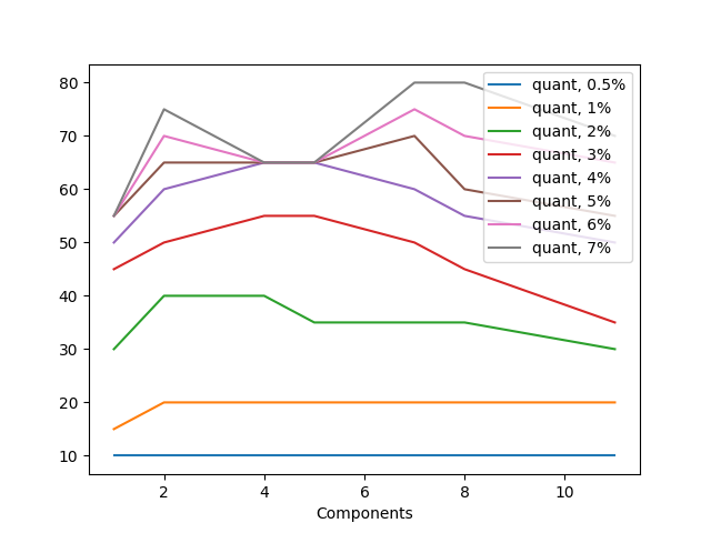
(a) IRF Method. Number of Components vs Percentage of Anomaly Detection. Original Labeling.

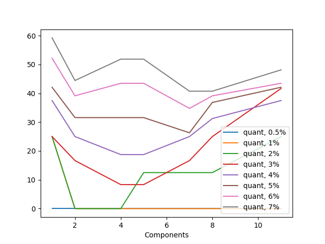
(b) IRF Method. Number of Components vs Percentage of False Positives. Original Labeling.

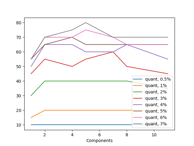
(c) DIRF Method. Number of Components vs Percentage of Anomaly Detection. Original Labeling.

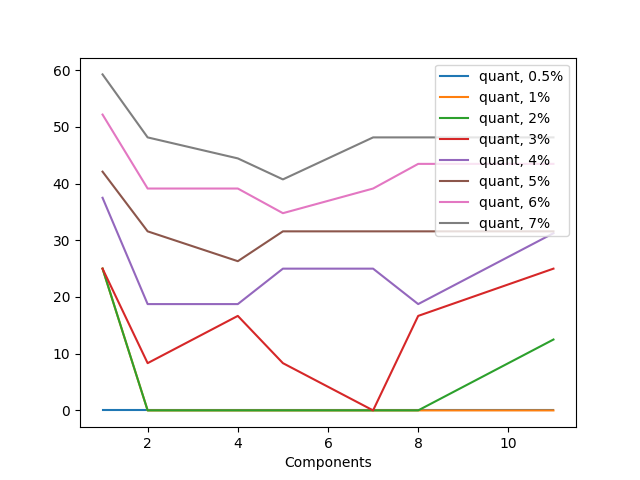
(d) DIRF Method. Number of Components vs Percentage of False Positives. Original Labeling.

Figure 4: Anomaly detection percentages for Example 1, Breast Cancer Diagnosis. All the graphics have the number of principal components in the $x$-axis and multiple curves for the quantiles to be used as a threshold. Figure (a) and (c) depict anomalies detected by both methods with the original labeling, while figures (b) and (d) display false positives introduced by both methods with the original labeling.

Example 1.

The first example uses the benchmark “Breast Cancer Wisconsin (Diagnosis) Data Set”, downloaded from https://www.kaggle.com/uciml/breast-cancer-wisconsin-data. Although the original data base contains 569 individuals, 213 patients (37.2%) were diagnosed with cancer. It is clear that the patients diagnosed with cancer can not be considered anomalies if the full data base is used for the analysis. Therefore the original data set was modified: the subset of healthy patients was left intact and 20 randomly chosen patients with cancer (3.5%) were chosen to complete the set.

Two labels were used, the diagnosis label coming from the original data set itself and a distance-based label computed according to Definition 10 with parameters $r=350$, $p=0.05$. The number of sampled trees (Bernoulli trials) is given by $K=2250$. The original dataset contains 32 columns, therefore we combine our technique with the PCA method (Principal Components Analysis); in this particular example we choose the 1, 2, 4, 5, 7, 8 and 11 first components. Our experiments show that both methods severely decay their quality from 11 components on, in particular both perform really poorly with the 32 components to be considered a viable option. Finally, the anomaly detection threshold quantiles are 0.5, 1, 2, 3, 4, 5, 6 and 7, which were chosen from observing the behavior of this particular case.

quantile [%]	0.5		1		2		3		4		5		6		7
components	A	F	A	F	A	F	A	F	A	F	A	F	A	F	A	F
1	0.0	0.0	0.0	0.0	0.0	0.0	0.0	0.0	0.0	0.0	0.0	0.0	0.0	0.0	0.0	0.0
2	0.0	0.0	0.0	0.0	0.0	0.0	-5.0	8.3	-5.0	6.3	0.0	0.0	0.0	0.0	5.0	-3.7
4	0.0	0.0	0.0	0.0	0.0	0.0	5.0	-8.3	0.0	0.0	-5.0	5.3	-5.0	4.3	-10.0	7.4
5	0.0	0.0	0.0	0.0	-5.0	12.5	0.0	0.0	5.0	-6.3	0.0	0.0	-10.0	8.7	-15.0	11.1
7	0.0	0.0	0.0	0.0	-5.0	12.5	-10.0	16.7	0.0	0.0	5.0	-5.3	5.0	-4.3	10.0	-7.4
8	0.0	0.0	0.0	0.0	-5.0	12.5	-5.0	8.3	-10.0	12.5	-5.0	5.3	5.0	-4.3	10.0	-7.4
11	0.0	0.0	0.0	0.0	-5.0	12.5	-10.0	16.7	-5.0	6.3	-10.0	10.5	0.0	0.0	0.0	0.0

Table 3: Table of differences IRF – DIRF, Breast Cancer Diagnosis, Example 1. All the values are the difference of percentages. The columns “A” and “F” stand for anomalies and false positives respectively.

The table 3 reports the difference of achievements attained by both methods when subtracting the DIRF from IRF. The predominance of negative and positive values in the columns “A” and “F” of the table 3 respectively, shows that the DIRF method performs better than the IRF method. Specially in the detection of false positives where DIRF performs significantly better than IRF: the former method presents convex curves, while the latter shows concave (or pseudo-convex) curves (see Figure 4).

Observe that the use of the quantiles is “dual” in the following sense. It is clear that all the curves tend to shift upwards when the quantile is amplified. This is good from the anomaly detection point of view but bad from the false positives inclusion point of view and it is hardly surprising: the larger the threshold, the more likely we are to detect more anomalies, but also the higher the price of including false positives. For our particular example using a quantile of 4% seems to be the “balanced choice”.

It must be observed that the quality of DIRF deteriorates with respect to IRF as we move along the diagonal of the table 3, in particular DIRF performs poorly with respect to IRF from 7 PCA components and from the 6% quantile on.

The same experiments were performed when using the artificial distance-based labeling introduced in Definition 10. It can be observed that both methods perform better for the anomaly detection, which is not unexpected because the DIRF method is strongly related to a distance function for anomalies, as shown in Theorem 9. However, both methods perform worse form the false positives inclusion point of view. Finally, the DIRF method performs better than the IRF method, although its superiority in the false positives inclusion is not as remarkable as in the first case.

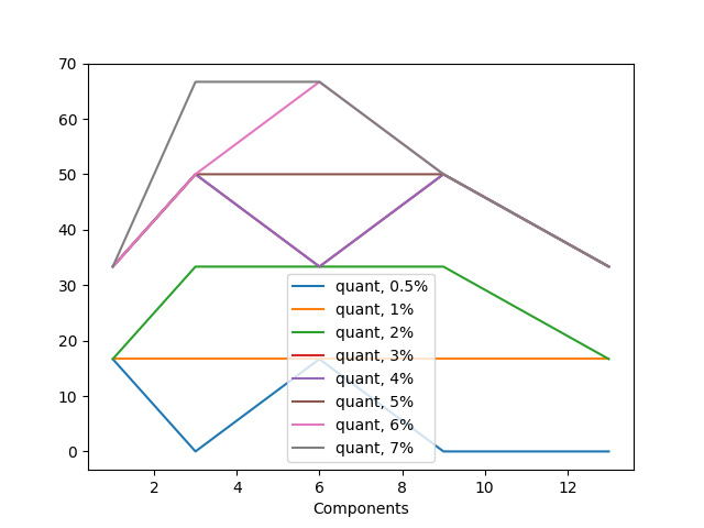
(a) IRF Method Number of Components vs Percentage of Anomaly Detection. Original Labeling.

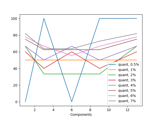
(b) IRF Method. Number of Components vs Percentage of False Positives. Original Labeling.

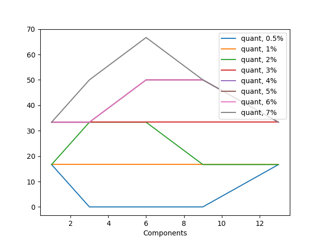
(c) DIRF Method. Number of Components vs Percentage of Anomaly Detection. Original Labeling.

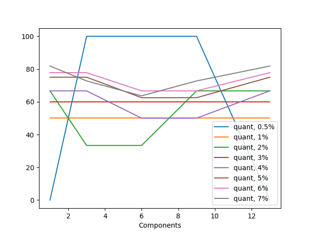
(d) DIRF Method. Number of Components vs Percentage of False Positives. Original Labeling.png

Figure 5: Anomaly detection percentages for Example 2, Lymphoma Diagnosis. All the graphics have the number of principal components in the $x$-axis and multiple curves for the quantiles to be used as a threshold. Figure (a) and (c) depict anomalies detected by both methods with the original labeling, while figures (b) and (d) display false positives introduced by both methods with the original labeling.

Example 2.

The second example uses a benchmark of lymphoma diagnosis, downloaded from www.kaggle.com. The dataset consists of 148 patients, with only 6 of them diagnosed having cancer, i.e. 4%.

Two labels were used, the diagnosis label coming from the original data set itself and a distance-based label computed according to Definition 10 with parameters $r=300$, $p=0.05$. The number of sampled trees (Bernoulli trials) is given by $K=1800$. The original dataset containes 18 columns, in contrast with Example 1, the application of PCA yields eigenvalues whose order of magnitude does not change as abruptly. Therefore, we work with the 1, 3, 6, 9 and 13 first components. Our experiments show that none of the methods has a good performance for any number of components and its quality decays even more from 6 components on (due to the noise introduced by the lower order components). Finally, the anomaly detection threshold quantiles are 0.5, 1, 2, 3, 4, 5, 6 and 7. These were chosen from observing the behavior of this particular case.

quantile [%]	0.5		1		2		3		4		5		6		7
components	A	F	A	F	A	F	A	F	A	F	A	F	A	F	A	F
1.0	0.0	0.0	0.0	0.0	0.0	0.0	0.0	0.0	0.0	0.0	0.0	0.0	0.0	0.0	0.0	0.0
3.0	0.0	0.0	0.0	0.0	0.0	0.0	16.7	-20.0	16.7	-16.7	16.7	-12.5	16.7	-11.1	16.7	-9.1
6.0	16.7	-100.0	0.0	0.0	0.0	0.0	0.0	0.0	-16.7	16.7	0.0	0.0	16.7	-11.1	0.0	0.0
9.0	0.0	0.0	0.0	0.0	16.7	-33.3	16.7	-20.0	0.0	0.0	0.0	0.0	0.0	0.0	0.0	0.0
13.0	-16.7	100.0	0.0	0.0	0.0	0.0	0.0	0.0	0.0	0.0	0.0	0.0	0.0	0.0	0.0	0.0

Table 4: Table of differences IRF – DIRF Lymphoma Diagnosis, Example 2. All the values are the difference of percentages. The columns “A” and “F” stand for anomalies and false positives respectively.

The table 4 reports the difference of achievements attained by both methods when subtracting the DIRF from IRF. Contrary to the previous example, there is a predominance of positive and negative values in the columns “A” and “F” of the table 4 respectively, showing that the IRF method performs better than the DIRF method with some few exceptions. This is also displayed in Figure 5. Nevertheless, we observe that the difference between methods is marginal.

As in the previous example, the 4% quantile seems to be the “balanced choice”. In particular DIRF and IRF perform identically from 9 PCA components on and from the 6% quantile on.

The same experiments were performed but using the artificial distance-based labeling introduced in Definition 10. In this case, both methods perform almost identically and worse than in the case of the original labeling.

5 Conclusions and Final Discussion.

The present work yields several conclusions listed below.

1. The IRF anomaly detection method introduced in [1, 2] has been mathematically analyzed. The well-posedness (Proposition 1) and the convergence of the algorithm (Corollary 3) have been established as well as the cardinality (size) of the probabilistic space (Theorem 4).

2. Under mild assumptions, it has been proved (see Theorem 13) that the computational cost of IRF method has order of magnitude $\mathcal{O}(N\log N)$, as claimed in [1, 2].

3. It has been shown that although the IRF method is well-defined, convergent and its target values $\{\bm{\mathbb{E}}(\mathsf{H}_{\mathbf{x}}):\mathbf{x}\in S\}$ are inconclusive when used as parameters for anomaly detection. (As shown in Lemma 5 and Theorem 6 an outlier $\mathbf{x}$ and a cluster point $\mathbf{y}$ can get the same expected height $\bm{\mathbb{E}}(\mathsf{H}_{x})=\bm{\mathbb{E}}(\mathsf{H}_{y})$.) Moreover, the IRF method can be deeply analyzed in the 1D case (Theorem 12) and it has been shown, from the theoretical point of view, that although it unquestionably detects outliers in this setting, its relationship with a notion of topological distance is not certain (see Theorem 9).

4. Taking advantage of the tractability of IRF for the 1D case, we have given theoretical estimates of the variance (Equation (20)) and derived the size of the sampling space (Equation (21)). This is necessary to guarantee confidence intervals for the empirically computed values of the expected heights. We have suggested a modification of the method in Section 3.4, named DIRF method (Directional Isolation Random Forest), whose differences with respect to the IRF method ar summarized in Table 2.

From the numerical examples in Section 4

1. There is definitely correlation bewteen the heights computed by the methods (IRF and DIRF), but it could be strong as in Example 1 or weak as in Example 2.

2. It is clear that the DIRF method is fully justified from the mathematical point of view which is desirable, however its relationship with a notion of distance is not certain (see the extent of Theorem 9) for multiple dimensions. In the examples we have seen IRF can perform better than DIRF, with a marginal difference. This is to be subject of extensive empirical evaluation in future work.

3. Both numerical examples may suggest that the adequate number of PCA components to introduce in the IRF and DIRF methods is one third of its total number of dimensions. Yet again, two experiments do not furnish enough numerical evidence to support such a conjecture, ergo this aspect needs to be further studied.

As for future work,

1. Although we have proved that the IRF method is inconclusive as a means to classify anomalies, experience shows that it can provide satisfactory results in practice, it follows that the method is correlated with anomalies. There are two possible approaches for enhancing the method:

   1. Find sufficient conditions for the data combinatorial configuration, to assure a quality certificate of IRF.

   2. Look for additional statistical parameters for anomaly detection (with computational cost no bigger than $\mathcal{O}(n\log n)$) to complement/contrast the information furnished by IRF.

   Both research lines will be explored in future work.

2. The mathematical analysis the methods presented in [15] and [16] will be pursued in future work, given that the performance of both is substantially superior to the original IRF. However, the probabilistic analysis will necessarily be different, because both references use random oblique hyperplanes for data separation, rather that axis-parallel as in IRF. This fact changes drastically the sampling space, from finite eligible directions in IRF, to uncountably many possible directions for the enhanced methods.

References

- [1] Liu FT, Ting KM, Zhou ZH. Isolation Forest. In: ; 2008: 413–422
- [2] Liu FT, Ting KM, Zhou ZH. Isolation-Based Anomaly Detection. TKDD 2012; 6: 3:1-3:39.
- [3] Angiulli F, Pizzuti C. Fast Outlier Detection in High Dimensional Spaces. In: Elomaa T, Mannila H, Toivonen H. , eds. Principles of Data Mining and Knowledge DiscoverySpringer Berlin Heidelberg; 2002; Berlin, Heidelberg: 15–27.
- [4] Bay SD, Schwabacher M. Mining Distance-Based Outliers in near Linear Time with Randomization and a Simple Pruning Rule. In: KDD ’03. Association for Computing Machinery; 2003; New York, NY, USA: 29–38
- [5] Knorr EM, Ng RT. Algorithms for Mining Distance-Based Outliers in Large Datasets. In: VLDB ’98. Morgan Kaufmann Publishers Inc.; 1998; San Francisco, CA, USA: 392–403.
- [6] Abe N, Zadrozny B, Langford J. Outlier Detection by Active Learning. In: KDD ’06. Association for Computing Machinery; 2006; New York, NY, USA: 504–509
- [7] Shi T, Horvath S. Unsupervised Learning With Random Forest Predictors. Journal of Computational and Graphical Statistics 2006; 15(1): 118-138. doi: 10.1198/106186006X94072
- [8] He Z, Xu X, Deng S. Discovering Cluster-Based Local Outliers. Pattern Recogn. Lett. 2003; 24(9–10): 1641–1650. doi: 10.1016/S0167-8655(03)00003-5
- [9] Criminisi A, Shotton J, Konukoglu E. Decision Forests: A Unified Framework for Classification, Regression, Density Estimation, Manifold Learning and Semi-Supervised Learning. Foundations and Trends® in Computer Graphics and Vision 2012; 7(2–3): 81–227. doi: 10.1561/0600000035
- [10] Ram P, Gray AG. Density Estimation Trees. In: KDD ’11. Association for Computing Machinery; 2011; New York, NY, USA: 627–635
- [11] Bandaragoda TR, Ting KM, Albrecht D, Liu FT, Wells JR. Efficient Anomaly Detection by Isolation Using Nearest Neighbour Ensemble. In: ; 2014: 698–705
- [12] Bandaragoda TR, Ting KM, Albrecht D, Liu FT, Zhu Y, Wells JR. Isolation-based anomaly detection using nearest-neighbor ensembles. Computational Intelligence 2018; 34(4): 968-998. doi: https://doi.org/10.1111/coin.12156
- [13] Thudumu S, Branch P, Jin J, Singh JJ. A comprehensive survey of anomaly detection techniques for high dimensional big data. Journal of Big Data 2020; 7(1): 1–30.
- [14] Chandola V, Banerjee A, Kumar V. Anomaly Detection: A Survey. ACM Comput. Surv. 2009; 41(3). doi: 10.1145/1541880.1541882
- [15] Liu FT, Ting KM, Zhou ZH. On Detecting Clustered Anomalies Using SCiForest. In: Balcázar JL, Bonchi F, Gionis A, Sebag M. , eds. Machine Learning and Knowledge Discovery in DatabasesSpringer Berlin Heidelberg; 2010; Berlin, Heidelberg: 274–290.
- [16] Hariri S, Kind M, Brunner R. Extended Isolation Forest. IEEE Transactions on Knowledge and Data Engineering 2021; 33(4): 1479–1489. Publisher Copyright: © 1989-2012 IEEE.doi: 10.1109/TKDE.2019.2947676
- [17] Murthy SK, Kasif S, Salzberg S. A System for Induction of Oblique Decision Trees. J. Artif. Int. Res. 1994; 2(1): 1–32.
- [18] Billinsgley P. Probability and Measure. Wiley Series in Probability and Mathematical StatisticsNew York: John Wiley Sons, Inc. . 1995.
- [19] Seidel R, Aragon CR. Randomized Search Trees. Algorithmica 1996; 16(4): 464–497.
- [20] Gross JL, Yellen J. Graph Theory and Its Applications, Second Edition (Discrete Mathematics and Its Applications). Chapman & Hall/CRC . 2005.
- [21] Thompson SK. Sampling. Wiley Series in Probability and StatisticsNew York: John Wiley Sons, Inc . 2012.
- [22] Bishop CM. Pattern Recognition and Machine Learning (Information Science and Statistics). Berlin, Heidelberg: Springer-Verlag . 2006.