Natural Alignment in Multi-Higgs Doublet Models

Abstract:

We present the complete set of continuous maximal symmetries that the potential of an $n$-Higgs Doublet Model ($n$HDM) should satisfy for natural Standard Model (SM) alignment. As a result, no large mass scales or fine-tuning is required for such alignment, which still persists even if these symmetries were broken softly by bilinear mass terms. In particular, the Maximal Symmetric $n$HDM (MS-$n$HDM) can provide both natural SM alignment and quartic coupling unification up to the Planck scale. Most remarkably, we show that the MS-2HDM is a very predictive extension of the SM governed by two only additional parameters: (i) the charged Higgs mass $M_{h^{\pm}}$ (or $m^{2}_{12}$) and (ii) $\tan\beta$, whilst the quartic coupling unification scale $\mu_{X}$ is predicted to assume two discrete values. With these two input parameters, the entire Higgs-mass spectrum of the model can be determined. Moreover, we obtain definite predictions of misalignment for the SM-like Higgs-boson couplings to the gauge bosons and to the quarks, which might be testable at future precision high-energy colliders.

1 Introduction

The quest for new physics beyond the Standard Model (SM), such as the exploration of non-standard scenarios with extended Higgs sectors, has strong theoretical and experimental motivations. The data collected from the CERN Large Hadron Collider (LHC) impose constraints over the coupling strengths of the Higgs boson, primarily to the electroweak (EW) gauge bosons ($Z,\,W^{\pm}$), which are very close to SM predictions [1, 2, 3]. This simple fact restricts severely the form of possible scalar-sector extensions of the SM.

An interesting class of Higgs-sector extensions is the one that augments the SM with $n\geq 2$ Higgs doublets, usually called the $n$-Higgs Doublet Model ($n$HDM). In the $n$HDM, the couplings of the SM-like Higgs boson to the EW gauge bosons ($Z,\,W^{\pm}$) must resemble those predicted by the SM, so as to be in agreement with the current Higgs signals at the LHC. This is only possible within the so-called SM alignment limit [4, 5, 6, 7, 8, 9, 10, 11, 12].

Achieving natural SM alignment via the implementation of symmetries has a historical background that reaches back as far as the introduction of the Cabibbo–Kobayashi–Maskawa (CKM) matrix [13, 14, 15]. If the three-generation of SM is complete, then the rotation embodied in the CKM matrix must be unitary. A similar approach utilises the so-called Glashow-Iliopoulos-Maiani (GIM) [16] mechanism to explain the smallness of the strangeness-changing interaction at the quantum level. Interestingly enough, the GIM mechanism requires the existence of the $c$-quark, and the conservation of strangeness by neutral currents naturally follows from the group structure and representation content of the SM. Later in 1977 [17], the necessary conditions for natural diagonal neutral currents in $Z$-boson interactions to all quark fields were proposed, where the solution was a generalization of the GlM scheme to many quark fields with two distinct charges. In the same period, equivalent conditions were derived by the authors in [18], who extended the concept of natural diagonal interactions to multi-Higgs-boson interactions to quarks. By 1996, it has been shown that the flavour-changing neutral current (FCNC) couplings of the neutral scalars of 2HDM can be related to elements of the CKM matrix with the help of symmetries of the model. From this brief historic review, it is evident that symmetries were always at the heart for realising natural SM alignment, i.e. having alignment or good agreement with SM predictions without decoupling of large mass scales or without resorting to ad-hoc arrangements among the parameters of the candidate new-physics theory [20, 21, 22, 7, 23, 24].

The potential of $n$HDMs contains a large number of SU(2)_L-preserving accidental symmetries as subgroups of the symplectic group Sp(2$n)$. The complete set of accidental symmetries that may occur in the tree-level scalar potential of $n$HDMs is classified in [19]. In particular, we have identified all accidental symmetries and derived the relationship among the theoretical parameters of the scalar potential for: (i) the Two Higgs Doublet Model (2HDM) and (ii) the Three Higgs Doublet Model (3HDM). We recover the maximum number of $13$ accidental symmetries for the 2HDM potential and for the first time, we presented the complete list of $40$ accidental symmetries for the 3HDM potential. Here, we Identify the complete set of continuous maximal symmetries for SM alignment in potential of $n$HDMs.

As an example, we discuss the phenomenological implications of natural SM alignment limit for Maximally Symmetric Two-Higgs Doublet Model (MS-2HDM) [25, 26]. This minimal model can account for a SM-like Higgs boson, and contains additionally one charged and two neutral scalars whose observation could be within reach of the LHC [10, 27, 28]. In MS-2HDM, the aforementioned SM alignment can emerge naturally as a consequence of a continuous symmetry Sp(4) $\cong$ SO$(5)$ in the Higgs sector [29, 8, 30, 31, 32]. The SO$(5)$ symmetry can be broken explicitly by two sources: (i) by renormalization-group (RG) effects and (ii) softly by the bilinear scalar mass term $m^{2}_{12}$. One of the interesting properties of this model is that all quartic couplings can unify at very large scales $\mu_{X}\sim 10^{11}\,$–$\,10^{20}$ GeV, for a wide range of $\tan\beta$ values and charged Higgs-boson masses. Specifically, we find that quartic coupling unification can emerge in two different conformally invariant points, where all quartic couplings vanish. The first conformal point is at relatively low-scale typically of order $\mu_{X}^{(1)}\sim 10^{11}$ GeV, while the second one is at high scale close to the Planck scale $\mu_{X}^{(2)}\sim 10^{19}$ GeV. Most remarkably, we show that the MS-2HDM is a very predictive extension of the SM which is governed by only two additional parameters: (i) the charged Higgs mass $M_{h^{\pm}}$ (or $m^{2}_{12}$) and (ii) the ratio $\tan\beta$ of the two Higgs-doublet vacuum expectation values, whereas the quartic coupling unification scale $\mu_{X}$ takes two discrete values as mentioned above. The two parameters, $M_{h^{\pm}}$ and $\tan\beta$, also suffice to determine the entire Higgs-mass spectrum of the model [32], for given values of $\mu^{(1,2)}_{X}$. These input parameters enable us to obtain definite predictions of misalignment for the SM-like Higgs-boson couplings to the gauge bosons and to the top- and bottom-quarks, which might be testable at future precision high-energy colliders.

These proceedings are organised as follows. Section 2 briefly reviews the basic features of the 2HDM and discusses the conditions for achieving exact SM alignment. In Section 3, we define the $n$HDMs in the bilinear scalar field formalism. Given that Sp(2$n)$ is the maximal symmetry of the $n$HDM potential, we present the complete set of continuous maximal symmetries for SM alignment that may take place in the $n$HDM potentials. Then, we introduce prime invariants to build potentials that are invariant under SU(2)_L-preserving continuous symmetries and present symmetries. In Section 4, we focus on MS-2HDM and outline the breaking pattern of the SO$(5)$ symmetry, which results from the soft-breaking mass $m^{2}_{12}$ and the RG effects. In this section, we also show that the running quartic couplings can be unified at two different conformally-invariant points and presents our misalignment predictions for Higgs-boson couplings to gauge bosons and top- and bottom-quarks. Finally, Section 5 contains our conclusions.

2 The 2HDM and SM Alignment

The Higgs sector of the 2HDM is described by two scalar SU(2) doublets,

$${\phi}_{i}\ =\ \left(\begin{matrix}\phi_{i}^{+}\\ \phi_{i}^{0}\end{matrix}\right),$$ (2.1)

with $i=1,2$. Both doublets have the same U(1)_Y-hypercharge quantum number, $Y_{\phi_{i}}={1/2}$. In terms of these doublets, the general SU(2)${}_{L}\times$U(1)_Y-invariant Higgs potential is given by

$$V = -\mu_{1}^{2}(\phi_{1}^{\dagger}\phi_{1})-\mu_{2}^{2}(\phi_{2}^{\dagger}\phi_{2})-\Big{[}m_{12}^{2}(\phi_{1}^{\dagger}\phi_{2})\>+\>{\rm H.c.}\Big{]}$$ (2.2)

$$+ \lambda_{1}(\phi_{1}^{\dagger}\phi_{1})^{2}+\lambda_{2}(\phi_{2}^{\dagger}\phi_{2})^{2}+\lambda_{3}(\phi_{1}^{\dagger}\phi_{1})(\phi_{2}^{\dagger}\phi_{2})+\lambda_{4}(\phi_{1}^{\dagger}\phi_{2})(\phi_{2}^{\dagger}\phi_{1})$$

$$+ \bigg{[}\,{1\over 2}\lambda_{5}(\phi_{1}^{\dagger}\phi_{2})^{2}+\lambda_{6}(\phi_{1}^{\dagger}\phi_{1})(\phi_{1}^{\dagger}\phi_{2})+\lambda_{7}(\phi_{1}^{\dagger}\phi_{2})(\phi_{2}^{\dagger}\phi_{2})\>+\>{\rm H.c.}\bigg{]},$$

where the mass terms $\mu^{2}_{1,2}$ and quartic couplings $\lambda_{1,2,3,4}$ are real parameters. Instead, the remaining mass term $m^{2}_{12}$ and the quartic couplings $\lambda_{5,6,7}$ are complex. Of these 14 theoretical parameters, only 11 are physical, since 3 parameters can be removed away using an SU(2) reparameterisation of the Higgs doublets $\phi_{1}$ and $\phi_{2}$ [22].

In the case of CP-conserving Type-II 2HDM, both scalar doublets $\phi_{1}$ and $\phi_{2}$ receive real and nonzero vacuum expectation values (VEVs). In detail, we have $\langle\phi_{1}^{0}\rangle=v_{1}/\sqrt{2}$ and $\langle\phi_{2}^{0}\rangle=v_{2}/\sqrt{2}$, where $t_{\beta}\equiv\tan\beta=v_{2}/v_{1}$ and the VEV of the SM Higgs doublet is $v\equiv{(v_{1}^{2}+v_{2}^{2})}^{1/2}$.

This model can account for only five physical scalar states: two CP-even scalars ($h$,$H$), one CP-odd scalar $(a)$ and two charged bosons ($h^{\pm}$). The masses of the $a$ and $h^{\pm}$ scalars are given by

$$M_{a}^{2}\ = \ M_{h^{\pm}}^{2}+{v^{2}\over 2}(\lambda_{4}-\lambda_{5}),$$

$$M_{h^{\pm}}^{2}\ = \ {m_{12}^{2}\over c_{\beta}s_{\beta}}-{v^{2}\over 2}(\lambda_{4}+\lambda_{5})+{v^{2}\over 2c_{\beta}s_{\beta}}(\lambda_{6}c_{\beta}^{2}+\lambda_{7}s_{\beta}^{2}),$$ (2.3)

where $s_{\beta}\equiv\sin{\beta}$, $c_{\beta}\equiv\cos{\beta}$.

The masses of the two CP-even scalars, $h$ and $H$ may be obtained by diagonalising the $2\times 2$ CP-even mass matrix $M^{2}_{S}$,

$$M_{S}^{2}=\left(\begin{matrix}{A}\,&\,{C}\\ {C}\,&\,{B}\end{matrix}\right),$$ (2.4)

which may explicitly be written down as

$$M_{S}^{2}\ =\ M_{a}^{2}\left(\begin{matrix}s_{\beta}^{2}&-c_{\beta}s_{\beta}\\ -c_{\beta}s_{\beta}&c_{\beta}^{2}\end{matrix}\right)+v^{2}\left(\begin{matrix}2\lambda_{1}c_{\beta}^{2}+\lambda_{5}s_{\beta}^{2}+2\lambda_{6}c_{\beta}s_{\beta}&\lambda_{34}c_{\beta}s_{\beta}+\lambda_{6}c_{\beta}^{2}+\lambda_{7}s_{\beta}^{2}\\ \lambda_{34}c_{\beta}s_{\beta}+\lambda_{6}c_{\beta}^{2}+\lambda_{7}s_{\beta}^{2}&2\lambda_{2}s_{\beta}^{2}+\lambda_{5}c_{\beta}^{2}+2\lambda_{7}c_{\beta}s_{\beta}\end{matrix}\right),$$

with $\lambda_{34}\equiv\lambda_{3}+\lambda_{4}$. The mixing angle $\alpha$ is required for the diagonalisation of $M_{S}^{2}$, which may be determined by

$$\tan 2\alpha\ =\ {2C\over A-B}.$$ (2.5)

In the so-called Higgs basis [20], the CP-even mass matrix $M_{S}^{2}$ given in (2.4) takes on the form

$${\widehat{M}_{S}}^{\,2} = \left(\begin{matrix}\widehat{A}&\widehat{C}\\ \widehat{C}&\widehat{B}\end{matrix}\right)=\left(\begin{matrix}{c_{\beta}}&{s_{\beta}}\\ -{s_{\beta}}&{c_{\beta}}\end{matrix}\right){M_{S}}^{2}\left(\begin{matrix}c_{\beta}&-{s_{\beta}}\\ s_{\beta}&c_{\beta}\end{matrix}\right),$$ (2.6)

with

$$\widehat{A} = 2v^{2}\left[c_{\beta}^{4}\lambda_{1}+s_{\beta}^{2}c_{\beta}^{2}\lambda_{345}+s_{\beta}^{4}\lambda_{2}+2c_{\beta}s_{\beta}\left(c_{\beta}^{2}\lambda_{6}+s_{\beta}^{2}\lambda_{7}\right)\right],$$

$$\widehat{B} = M_{a}^{2}+\lambda_{5}v^{2}+2v^{2}\left[s_{\beta}^{2}c_{\beta}^{2}\left(\lambda_{1}+\lambda_{2}-\lambda_{345}\right)-c_{\beta}s_{\beta}\left(c_{\beta}^{2}-s_{\beta}^{2}\right)\left(\lambda_{6}-\lambda_{7}\right)\right],$$ (2.7)

$$\widehat{C} = v^{2}\left[s_{\beta}^{3}c_{\beta}\left(2\lambda_{2}-\lambda_{345}\right)-c_{\beta}^{3}s_{\beta}\left(2\lambda_{1}-\lambda_{345}\right)+c_{\beta}^{2}\left(1-4s_{\beta}^{2}\right)\lambda_{6}+s_{\beta}^{2}\left(4c_{\beta}^{2}-1\right)\lambda_{7}\right].$$

The SM Higgs field may now be identified by the linear field combination,

$$H_{\text{SM}}\ =\,H\cos(\beta-\alpha)\,+\,h\sin(\beta-\alpha).$$ (2.8)

To this extend, one may obtain the SM-normalised couplings of the CP-even scalars, $h$ and $H$, to the EW gauge bosons ($V=W^{\pm},Z$) as follows:

$$g_{hVV}=\sin(\beta-\alpha),\qquad g_{HVV}=\cos(\beta-\alpha).$$ (2.9)

In similar way, the SM-normalised couplings of the CP-even scalars to quarks may be derived. In Table 1, these couplings are displayed.

S			$g_{SVV}$ ($V=W^{\pm},Z$)				$g_{Suu}$				$g_{Sdd}$
$h$			$\sin(\beta-\alpha)$				$\sin(\beta-\alpha)+t^{-1}_{\beta}\cos(\beta-\alpha)$				$\sin(\beta-\alpha)-t_{\beta}\cos(\beta-\alpha)$
$H$			$\cos(\beta-\alpha)$				$\cos(\beta-\alpha)-t^{-1}_{\beta}\sin(\beta-\alpha)$				$\cos(\beta-\alpha)+t_{\beta}\sin(\beta-\alpha)$

Table 1: Tree-level couplings of CP-even scalar boson $S$ (with$\,S=h,\,H$) to the EW gauge bosons ($Z$, $W^{\pm}$) and to up-type and down-type quarks in the Type-II 2HDM.

From Table 1, we observe that there are two scenarios to realise the SM alignment limit:

• SM-like  $H$ scenario: $M_{H}\approx 125\text{~{}GeV},\,\cos(\beta-\alpha)\to 1,\,\,\text{with}\,\,\beta\approx\alpha$.

• SM-like  $h$ scenario: $M_{h}\approx 125\text{~{}GeV},\,\sin(\beta-\alpha)\to 1,\,\,\text{with}\,\,\beta-\alpha\approx\pi/2$.

In these limits, the CP-even $H\,(h)$ scalar couples to the EW gauge bosons with coupling strength exactly as that of the SM Higgs boson, while $h\,(H)$ does not couple to them at all [8]. In the above two scenarios, the SM-like Higgs boson mass is identified with the $\sim 125~{}\text{GeV}$ resonance observed at the LHC [34, 35]. In the literature, the neutral Higgs partner $(H)$ in the SM-like $h$ scenario is usually termed the heavy Higgs boson. Instead, in the SM-like $H$ scenario, the partner particle $h$ can only have a mass smaller than $\sim\,125~{}\text{GeV}$  [9]. In our study, we adopt the SM-like $H$ scenario, but the partner $h$ would be either heavier or lighter than the observed scalar resonance at the LHC.

In (2), the SM alignment limit $\cos(\beta-\alpha)~{}\to~{}1$ can be achieved in two different approaches: (i) $\widehat{C}\to 0$ and (ii) $M_{h^{\pm}}\!\sim\!M_{a}\gg v$. The first realisation (i) does not depend on the choice of the non-SM scalar masses, such as $M_{h^{\pm}}$ and $M_{a}$, whereas the second one (ii) is only possible in the well-known decoupling limit [20, 21, 22]. In the first realisation, SM alignment is obtained by setting $\widehat{C}=0$, which in turn implies the condition [8]:

$$\lambda_{7}t_{\beta}^{4}-\left(2\lambda_{2}-\lambda_{345}\right)t_{\beta}^{3}+3\left(\lambda_{6}-\lambda_{7}\right)t_{\beta}^{2}+\left(2\lambda_{1}-\lambda_{345}\right)t_{\beta}-\lambda_{6}\ =\ 0.$$ (2.10)

Barring fine-tuning among quartic couplings, (2.10) leads to the two different types of constraints:

1. $$\lambda_{1}\ =\ \lambda_{2}\ =\ \frac{\lambda_{345}}{2},\qquad\lambda_{6}\ =\ \lambda_{7}\ =\ 0,$$ (2.11)

   which are independent of $\tan\beta$ and non-standard scalar masses. In this case, the masses of both CP-even scalars in the alignment limit are given by

   $$M_{H}^{2}\ =\ 2v^{2}\left(\lambda_{1}c_{\beta}^{4}+\lambda_{345}s_{\beta}^{2}c_{\beta}^{2}+\lambda_{2}s_{\beta}^{4}\right)\ \equiv\ 2\lambda_{\text{SM}}v^{2},$$ (2.12)

   $$M_{h}^{2}\ =\ M_{a}^{2}+v^{2}\lambda_{5}+2v^{2}s_{\beta}^{2}c_{\beta}^{2}\left(\lambda_{1}+\lambda_{2}-\lambda_{345}\right).$$ (2.13)

2. $$\tan\beta=1\>,\quad\lambda_{1}\ =\ \lambda_{2},\quad\ \lambda_{3},\quad\ \lambda_{4},\quad\ \lambda_{5},\quad\lambda_{6}\ =\ \lambda_{7}\ ,$$ (2.14)

   where the masses of both CP-even scalars in the alignment limit may take the following forms,

   $$M_{H}^{2}\ =\ 2v^{2}\left(\lambda_{1}+\lambda_{2}+\lambda_{345}+2(\lambda_{6}+\lambda_{7})\right)\ ,$$ (2.15)

   $$M_{h}^{2}\ =\ M_{a}^{2}+\lambda_{5}v^{2}+2v^{2}\left(\lambda_{1}+\lambda_{2}-\lambda_{345}\right)\ .$$ (2.16)

Note that the constraints given in 2 represent a particular limit of the constraints 1. As we will discuss further in Section 3, these constraints mainly lead to an inert Type-I 2HDM in the Higgs basis, for which SM alignment is automatic thanks to an unbroken $Z_{2}$ symmetry.

In the second realisation for the SM alignment limit $\cos(\beta-\alpha)\to 1$ mentioned above, i.e.  $M_{h^{\pm}}\!\sim\!M_{a}\gg v$, we may simplify matters by expanding $M^{2}_{H,h}$ in powers of $v/M_{a}\ll 1$. So, we may find [8]

$$M_{H}^{2}\ \simeq\ 2\lambda_{\text{SM}}v^{2}-{v^{4}s_{\beta}^{2}c_{\beta}^{2}\over M_{a}^{2}+\lambda_{5}v^{2}}\,\Big{[}s_{\beta}^{2}\left(2\lambda_{2}-\lambda_{345}\right)-c_{\beta}^{2}\left(2\lambda_{1}-\lambda_{345}\right)\Big{]}^{2}\,,$$ (2.17)

$$M_{h}^{2}\ \simeq\ M_{a}^{2}+\lambda_{5}v^{2}\ \gg\ v^{2}.$$ (2.18)

Note that for large values of $\tan\beta$, the phenomenological properties of the $H$-boson become more and more close to those of the SM Higgs boson [7, 6]. Since we are interested in analysing the misalignment of the $H$-boson couplings from their SM values, we follow an approximate approach inspired by the seesaw mechanism [36]. Particularly, we will express all the $H$-boson couplings in terms of the light-to-heavy scalar-mixing parameter $\theta_{\mathcal{S}}\equiv\widehat{C}/\widehat{B}$. Thus, operating (2.5) for the hatted quantities and employing ${\widehat{A}}\gg{\widehat{C}}$, the following approximate analytic expressions may be derived

$$g_{HVV} \simeq 1-{\theta_{\mathcal{S}}^{2}\over 2},$$ (2.19a)

$$g_{hVV} \simeq-{\theta_{\mathcal{S}}}\ =\ {v^{2}c_{\beta}s_{\beta}\over M_{a}^{2}+v^{2}\lambda_{5}}\,\Big{[}\,c_{\beta}^{2}\left(2\lambda_{1}-\lambda_{345}\right)-s_{\beta}^{2}\left(2\lambda_{2}-\lambda_{345}\right)\Big{]}.$$ (2.19b)

Given the narrow experimental limits on the deviation of $g_{HVV}$ from 1, one must have the parameter $\theta_{\mathcal{S}}\ll 1$, which justifies our seesaw-inspired approximation. In fact, the mixing parameter $\theta_{\mathcal{S}}$ vanishes in the exact SM alignment limit as $\alpha\to\beta$.

To this extent, we derive approximate analytic expressions for the $h$- and $H$-boson couplings to up- and down-type quarks. To leading order in the light-to-heavy scalar-mixing $\theta_{\mathcal{S}}$, these are given by

$$g_{Huu} \simeq 1+{t^{-1}_{\beta}}\,{\theta_{\mathcal{S}}},\qquad\qquad g_{Hdd}\simeq 1-{\theta_{\mathcal{S}}}\,{t_{\beta}},$$ (2.20)

$$g_{huu} \simeq-{\theta_{\mathcal{S}}}+{t^{-1}_{\beta}},\qquad\qquad g_{hdd}\simeq-{\theta_{\mathcal{S}}}-{t_{\beta}}.$$

In the SM alignment limit, we have $g_{Huu}\,\to\,1$ 1 and $g_{Hdd}\to$ 1. Obviously, any deviation of these couplings from their SM values is governed by quantities $\tan\beta$ and $\theta_{\mathcal{S}}$.

In this study, our primary interest lies in natural realisations of SM alignment, for which neither a mass hierarchy $M_{h^{\pm}}\!\sim\!M_{a}\gg v$, nor a fine-tuning among the quartic couplings would be necessary. To this end, one is therefore compelled to identify possible maximal symmetries of the $2$HDM potential that would impose the condition stated in (2.10). Thereafter, this result may be generalized for $n$HDM potential to achieve the SM alignment limit. In the next section, we will show how SM alignment can be achieved naturally by virtue of accidental continuous symmetries imposed on the theory.

3 Multi-Higgs Doublet Models and Natural Alignment

The $n$HDMs contains $n$ scalar doublet fields, $\phi_{i}\,\,(i=1,2,\cdots,n)$, which all have the same U(1)_Y-hypercharge quantum number. The most general SU(2)${}_{L}\times$U(1)_Y invariant $n$HDM potential may conventionally be given as [37]:

$$V_{n}=\ \displaystyle\sum_{i,j=1}^{n}\,m_{ij}^{2}\,(\phi_{i}^{\dagger}\phi_{j})+\ \displaystyle\sum_{i,j\,k,l=1}^{n}\,\lambda_{ijkl}\,(\phi_{i}^{\dagger}\phi_{j})(\phi_{k}^{\dagger}\phi_{l}),$$ (3.1)

with $\lambda_{ijkl}=\lambda_{klij}$. In general, the above potential contains $n^{2}$ physical mass terms and $n^{2}(n^{2}+1)/2$ physical quartic couplings.

An equivalent way to write the $n$HDM potential is based on the so-called bilinear field formalism [39, 40, 41, 42]. To this end, we first define a $4n$-dimensional ($4n$-D) complex ${\bm{\Phi}}_{n}$-multiplet as

$${\bm{\Phi}}_{2}^{\mathsf{T}}=\begin{pmatrix}\phi_{1},\,\phi_{2},\,\tilde{\phi_{1}},\,\tilde{\phi_{2}}\,\end{pmatrix}^{\mathsf{T}},$$

$${\bm{\Phi}}_{3}^{\mathsf{T}}=\begin{pmatrix}\phi_{1},\,\phi_{2},\,\phi_{3},\,\tilde{\phi_{1}},\,\tilde{\phi_{2}},\,\tilde{\phi_{3}}\,\end{pmatrix}^{\mathsf{T}},$$

$$\cdots$$

$${\bm{\Phi}}_{n}^{\mathsf{T}}=\begin{pmatrix}\phi_{1},\,\phi_{2},\,\phi_{3},\,\cdots,\tilde{\phi_{1}},\,\tilde{\phi_{2}},\,\tilde{\phi_{3}},\,\cdots\end{pmatrix}^{\mathsf{T}},$$ (3.2)

where $\sigma^{1,2,3}$ are the Pauli matrices and $\tilde{\phi_{i}}=i\sigma^{2}\phi_{i}^{*}$ are the U(1)_Y hypercharge-conjugate of $\phi_{i}$. Observe that the ${\bm{\Phi}}_{n}$-multiplet transforms covariantly under an SU(2$)_{L}$ gauge transformation as,

$${\bm{\Phi}}_{n}\to\text{U}_{L}{\bm{\Phi}}_{n},\quad\text{U}_{L}\in\text{SU(2)}_{L}.$$ (3.3)

Additionally, this multiplet satisfies the following Majorana-type property [42],

$${\bm{\Phi}}_{n}=C{{\bm{\Phi}}_{n}^{*}},$$ (3.4)

where $C=\sigma^{2}\otimes{\bf{1}}_{n}\otimes\sigma^{2}$ ($C=C^{-1}=C^{*}$) is the charge conjugation operator and ${\bf{1}}_{n}$ is the $n\times n$ identity matrix.

With the help of the ${\bm{\Phi}}_{n}$-multiplet, we may now define the bilinear fields vector [41, 29, 42],

$$R_{n}^{A}\equiv{\bm{\Phi}}_{n}^{\dagger}{\Sigma}^{A}_{n}{\bm{\Phi}}_{n},$$ (3.5)

with ${A}=0,1,2,\cdots,n(2n-1)-1$. Notice that $n(2n-1)$-vector $R_{n}^{A}$ is invariant under SU(2)_L transformations thanks to (3.3).

The ${\Sigma}^{A}_{n}$ matrices have $4n\times 4n$ elements and can be expressed in terms of double tensor products as

$${\Sigma}^{A}_{n}=\left(\sigma^{0}\otimes t_{S}^{a}\otimes\sigma^{0},\quad\sigma^{i}\otimes t_{A}^{b}\otimes\sigma^{0}\right),$$ (3.6)

where $t_{S}^{a}$ and $t_{A}^{b}$ are the symmetric and anti-symmetric matrices of the SU($n$) symmetry generators, respectively.

With the aid of $n(2n-1)$-vector $R_{n}^{A}$, the potential $V_{n}$ for an $n$HDM can be written down in the quadratic form as

$$V_{n}=-\dfrac{1}{2}M^{n}_{A}R_{n}^{A}+\dfrac{1}{4}L^{n}_{{A}{A^{\prime}}}R_{n}^{A}R_{n}^{{A^{\prime}}},$$ (3.7)

where $M^{n}_{A}$ is the $1\times n(2n-1)$-dimensional mass matrix and $L^{n}_{{A}{A^{\prime}}}$ is a quartic coupling matrix with $n(2n-1)\times n(2n-1)$ entries. Evidently, for a U(1$)_{Y}$-invariant $n$HDM potential the first $n^{2}$ elements of $M^{n}_{A}$ and $n^{2}\times n^{2}$ elements of $L^{n}_{{A}{A^{\prime}}}$ are only relevant, since the other U(1$)_{Y}$-violating components vanish.

The gauge-kinetic term $T_{n}$ is given by

$$T_{n}=\frac{1}{2}(D_{\mu}{\bm{\Phi}}_{n})^{\dagger}(D^{\mu}{\bm{\Phi}}_{n}),$$ (3.8)

where the covariant derivative, $D_{\mu}$, in the ${\bm{\Phi}}_{n}$ space is

$$D_{\mu} =\sigma^{0}\otimes{\bf{1}}_{n}\otimes\sigma^{0}\,\partial_{\mu}\>+\>i\frac{g_{w}}{2}\sigma^{0}\otimes{\bf{1}}_{n}\otimes\sigma^{i}\,W_{\mu}^{i}\>+\>i{g_{Y}\over 2}\,B_{\mu}\,\sigma^{3}\otimes{\bf{1}}_{n}\otimes\sigma^{0}\;.$$ (3.9)

In the limit $g_{Y}\to 0$, the gauge-kinetic term is invariant under $\text{Sp}(2n)/Z_{2}\otimes\text{SU}(2)_{L}$ transformations of the multiplet-$\bm{\Phi}_{n}$. In general, the maximal symmetry group acting on the ${\bm{\Phi}}_{n}$-space in the $n$HDM potentials is

$$\text{G}_{\mathsf{n\text{-HDM}}}^{{\bm{\Phi}}_{n}}=\text{Sp}(2n)/Z_{2}\otimes\text{SU}(2)_{L},$$

which leaves the local SU($2)_{L}$ gauge kinetic term of ${\bm{\Phi}}_{n}$ canonical. The local $SU(2)_{L}$ group generators can be represented as $\sigma^{0}\otimes{\bf{1}}_{n}\otimes(\sigma^{1,2,3}/2)$, that commute with all generators of Sp($2n)$.

Knowing that Sp(2$n)$ is the maximal symmetry group allows us to classify all SU(2)_L-preserving accidental symmetries of $n$HDM potentials. The potential of $n$HDMs contains a large number of SU(2)_L-preserving accidental symmetries as subgroups of the symplectic group Sp(2$n)$. The complete set of accidental symmetries that may occur in the tree-level scalar potential of $n$HDMs is classified in [19]. In the same context, we identify the complete set of continuous maximal symmetries that an $n$HDM potential must obey for having SM alignment. First, we will presnt all possible maximal SM-alignment symmetries for the $2$HDM potential, and then we will generalize these for $n$HDM potentials.

In Section 2, it has been shown that the SM alignment in the $2$HDM potential can be achieved when the constraint (2.10) is fulfilled. This constraint may be due to some accidental continuous symmetry imposed on the model. Given all accidental continuous symmetries [29, 19], we may look for those symmetries that would impose the condition stated in (2.10). Along these lines, the following three symmetries for SM alignment have been identified satisfying the condition (2.11):

(i) $$\text{SO(2)}:\quad\mu_{1}^{2}=\mu_{2}^{2};\quad m_{12}^{2}=0;\quad\lambda_{1}\ =\ \lambda_{2}\ =\ \lambda_{345}/2\,;\quad\lambda_{6,7}\ =\ 0,$$ (3.10a)

(ii) $$\text{SU(2)}:\quad\mu_{1}^{2}=\mu_{2}^{2};\quad m_{12}^{2}=0;\quad\lambda_{1}\ =\ \lambda_{2}\ =\ \lambda_{34}/2;\quad\ \lambda_{5,6,7}\ =\ 0,$$ (3.10b)

(iii) $$\text{Sp(4)}:\quad\mu_{1}^{2}=\mu_{2}^{2};\quad m_{12}^{2}=0;\quad\lambda_{1}\ =\ \lambda_{2}\ =\ \lambda_{3}/2;\quad\lambda_{4,5,6,7}\ =\ 0.$$ (3.10c)

In the above list, having SM alignment limit is independent of values of $\tan\beta$, and the values of the soft-breaking bilinear mass terms $\mu^{2}_{1,2}$ and $m^{2}_{12}$. In addition to above symmetries, in the weak basis $\lambda_{6}=\lambda_{7}$, the possibility $\tan\beta=1$ gives rise to the following symmetries for SM alignment (2.14):

(a) $$\text{CP2}:\,\mu_{1}^{2}=\mu_{2}^{2};\,m_{12}^{2}=0;\,\lambda_{1}=\lambda_{2};\,\lambda_{3};\,\lambda_{4};\,\lambda_{5};\,\lambda_{6,7}=0,$$ (3.11a)

(b) $$(\text{CP1}\rtimes\,S_{2})\otimes\text{ Sp(2)}_{\phi_{1}+\phi_{2}}:\,\mu_{1}^{2}=\mu_{2}^{2};\,m_{12}^{2};\,\lambda_{1}=\lambda_{2};\,\lambda_{3};\,\lambda_{4}=\lambda_{5};\,\lambda_{6}=\lambda_{7},$$ (3.11b)

(c) $$(S_{2}\rtimes Z_{2})\otimes\text{Sp(2)}_{\phi_{1}+\phi_{2}}:\,\mu_{1}^{2}=\mu_{2}^{2};\,m_{12}^{2}=0;\,\lambda_{1}=\lambda_{2};\,\lambda_{3};\,\lambda_{5}=\pm\lambda_{4};\,\lambda_{6,7}=0,$$ (3.11c)

(d) $$\text{U(1)}_{\text{}}\otimes\text{Sp(2)}_{\phi_{1}\phi_{2}}:\,\mu_{1}^{2}=\mu_{2}^{2};\,m_{12}^{2}=0;\,\lambda_{1}=\lambda_{2}=\lambda_{3}/2;\,\lambda_{4};\,\lambda_{5,6,7}\ =\ 0,$$ (3.11d)

(e) $$S_{2}\,\otimes\text{Sp(2)}_{\phi_{1}}\otimes\text{Sp(2)}_{\phi_{2}}:\,\mu_{1}^{2}=\mu_{2}^{2};\,m_{12}^{2}=0;\,\lambda_{1}=\lambda_{2};\,\lambda_{3};\;\,\lambda_{4,5,6,7}=0,$$ (3.11e)

where the subscript ${\phi_{1}+\phi_{2}}$ shows an Sp(2) transformation that acts on both $(\phi_{1},i\sigma^{2}\phi_{1}^{*})^{\mathsf{T}}$ and $(\phi_{2},i\sigma^{2}\phi_{2}^{*})^{\mathsf{T}}$. Additionally, the subscript ${\phi_{1}\phi_{2}}$ denotes an Sp(2) transformation acting on $(\phi_{1},i\sigma^{2}\phi_{2}^{*})^{\mathsf{T}}$.

It is important to note here that SM alignment does not get spoiled when $m^{2}_{12}\neq 0$ for the symmetries (a)–(e) stated in (3.11). Nevertheless, one should always have $\mu^{2}_{1}=\mu^{2}_{2}$ at the tree level in order to satisfy the minimization conditions for the 2HDM potential [33]. In the so-called Higgs basis, all symmetries in (3.11), with exception the one in (b), lead to restricted forms of inert Type-I 2HDM potentials, for which SM alignment is automatic as a result of an unbroken $Z_{2}$ symmetry.

To sum up, the set of symmetries in  (3.10) satisfy alignment conditions naturally without imposing any constraint on the values of $\tan\beta$, nor on the bilinear mass terms $\mu^{2}_{1,2}$ and $m^{2}_{12}$. However, in the set of symmetries  (3.11), exact alignment can be achieved only for the specific value $\tan\beta=1$ and for $\mu^{2}_{1}=\mu^{2}_{2}$.

Having obtained these symmetries, it is straightforward to generalize these results to the $n$HDM potentials, with $n>2$. Of the $n$ scalar doublets, we assume that a number $m<n$ correspond to inert doublets, which do not participate in electroweak symmetry breaking (EWSB), need to be treated differently.

The full scalar potential $V$ of a naturally aligned $n$HDM may be written down as a sum of three terms:

$$V=V_{sym}+V_{inert}+\Delta V.$$ (3.12)

We first construct the symmetry-constrained part of the scalar potential $V_{sym}$ in terms of fundamental building blocks that respect the symmetries. Here, we introduce the invariants $S_{n}$, $D_{n}^{2}$ and $T_{n}^{2}$. In detail, $S_{n}$ is defined as

$$S_{n}\ =\ {\bm{\Phi}}_{n}^{\dagger}{\bm{\Phi}}_{n},$$ (3.13)

which is invariant under both the SU($n)_{L}\otimes$U(1)_Y gauge group and Sp(2$n$). Moreover, we define the SU(2)_L-covariant quantity $D^{a}_{n}$ in the HF space as

$$D_{n}^{a}\ =\ {{\Phi}}^{\dagger}\sigma^{a}{{\Phi}},$$ (3.14)

with $\Phi=(\phi_{1},\phi_{2},\dots,\phi_{n})^{\mathsf{T}}$. Under an SU(2)_L gauge transformation, $D^{a}_{n}\to D_{n}^{\prime a}=O^{ab}D_{n}^{b}$, where $O\in$ SO(3). Hence, the quadratic quantity $D_{n}^{2}\equiv D^{a}_{n}D^{a}_{n}$ is both gauge and SU($n$) invariant. Finally, we define the auxiliary quantity $T_{n}$ in the HF space as

$$T_{n}\ =\ \Phi\Phi^{\mathsf{T}},$$ (3.15)

which transforms as a triplet under SU(2)_L, i.e. $T_{n}\,\to\,T_{n}^{\prime}=U_{L}T_{n}U_{L}^{\mathsf{T}}$. As a consequence, a proper prime invariant may be defined as $\,T_{n}^{2}\equiv\text{Tr}(TT^{*})$, which is also both gauge and SO($n$) invariant.

Thus, we can construct the symmetry-constrained part of the scalar potential $V_{sym}$ in terms of prime invariants in the following form,

$$V_{sym}=-\mu^{2}S_{n}+\lambda_{S}S_{n}^{2}+\lambda_{D}D_{n}^{2}+\lambda_{T}T_{n}^{2}.$$ (3.16)

Obviously, the simplest form of the $n$HDM potentials belong to the maximal symmetry Sp(2$n$), which has the same form as the SM potential,

$$V_{\text{SM}}=-\mu^{2}\left(\phi^{\dagger}\phi\right)+\lambda\left(\phi^{\dagger}\phi\right)^{2},$$

with a single mass term and a single quartic coupling. For example, the 2HDM Sp(4)${/Z_{2}}$-invariant potential, the so called MS-2HDM is

$$V_{\text{MS-2HDM}}\ =\ -\mu_{1}^{2}\left(\left|\phi_{1}\right|^{2}\>+\>\left|\phi_{2}\right|^{2}\right)+\lambda_{1}\left(\left|\phi_{1}\right|^{2}+\left|\phi_{2}\right|^{2}\right)^{2},$$ (3.17)

where the parameters have the following relations,

$$\mu_{1}^{2}=\mu_{2}^{2},\quad m_{12}^{2}=0,\quad 2\lambda_{2}=2\lambda_{1}=\lambda_{3},\quad\lambda_{4}=\text{Re}(\lambda_{5})=\lambda_{6}=\lambda_{7}=0.$$ (3.18)

The above potential is a functional of a single symmetric block, $S_{2}$, i.e. $V_{\text{MS-2HDM}}=V[S_{2}]$.

In addition, the potential term $V_{inert}$ in (3.12) represents the inert scalar sector of the theory consists of $m$ inert Higgs doublets $\widehat{\phi}_{\hat{i}}$ (with $\hat{i}=\hat{1},\hat{2},\cdots,\hat{m}$), for which $\langle\widehat{\phi}_{\hat{i}}\rangle=0$, and $N_{H}\equiv n-m$ Higgs doublets $\phi_{i}$ (with $i=1,2,\cdots,N_{H}$) which generally take part in EWSB with non-zero VEVs, $\langle\phi_{i}\rangle\neq 0$. The potential term $V_{inert}$ takes on the form

$$V_{\rm inert} = \widehat{m}_{\hat{i}\hat{j}}^{2}\widehat{\phi}_{\hat{i}}^{\dagger}\widehat{\phi}_{\hat{j}}+\lambda_{\hat{i}\hat{j}\hat{k}\hat{l}}\left(\widehat{\phi}_{\hat{i}}^{\dagger}\widehat{\phi}_{\hat{j}}\right)\left(\widehat{\phi}_{\hat{k}}^{\dagger}\widehat{\phi}_{\hat{l}}\right)+\lambda_{\hat{i}\hat{j}kl}\left(\widehat{\phi}_{\hat{i}}^{\dagger}\widehat{\phi}_{\hat{j}}\right)\left(\phi_{k}^{\dagger}\phi_{l}\right)$$ (3.19)

$$+ \lambda_{i\hat{j}\hat{k}l}\left(\phi_{i}^{\dagger}\widehat{\phi}_{\hat{j}}\right)\left(\widehat{\phi}_{\hat{k}}^{\dagger}\phi_{l}\right)+\left[\lambda_{i\hat{j}k\hat{l}}\left(\phi_{i}^{\dagger}\widehat{\phi}_{\hat{j}}\right)\left(\phi_{k}^{\dagger}\widehat{\phi}_{\hat{l}}\right)+{\rm H.c.}\right],$$

which must remain invariant under the $Z^{I}_{2}$ symmetry,

$$Z^{I}_{2}:~{}\phi_{i}~{}\to~{}\phi_{i},~{}\widehat{\phi}_{\hat{j}}~{}\to-\widehat{\phi}_{\hat{j}}.$$ (3.20)

The $m\times m$ matrix $\widehat{m}_{\hat{i}\hat{j}}^{2}$ is taken to be positive definite, so as to avoid spontaneous EWSB.

Consequently, $Z^{I}_{2}$ should always be contained in the $\mathcal{D}$ symmetry group of the inert scalar sector, i.e. $Z^{I}_{2}\subset\mathcal{D}$. Notice that, in the case of Type-I inert 2HDM, $Z^{I}_{2}$ can be extended by another $Z_{2}^{\text{EW}}\sim S_{2}$, namely the Permutation group which consists of the field permutation: $(\phi_{1},\phi_{2})\to(\phi_{2},\phi_{1})$. In general, the combined action $Z_{2}^{\text{EW}}\times Z^{I}_{2}$ enforces SM alignment in the $n$HDM, even beyond the tree-level approximation [30]. Note that in the 2HDM the constraint arising from $S_{2}\times Z^{I}_{2}$ symmetry meets the alignment conditions given in Eq.(2.14), with $\lambda_{6}=\lambda_{7}=0$.

Finally, the third term $\Delta V$ in (3.12) contains the soft-symmetry breaking mass parameters of the EWSB sector and is given by

$$\Delta V\ =\ \displaystyle\sum_{i,j=1,2}^{N_{H}}\,m_{ij}^{2}\,(\phi_{i}^{\dagger}\phi_{j}).$$ (3.21)

where $m_{ij}^{2}$ is in general a Hermitian $N_{H}\times N_{H}$ matrix, with at least one negative eigenvalue in order to trigger EWSB. We assume that the soft-symmetry breaking mass matrix $m_{ij}^{2}$ has no particular discrete symmetry structure.

Therefore, the symmetries for SM alignment acting on the EWSM sector are [30]

$$\text{(i) Sp(2}N_{H})\times\mathcal{D}\;,\qquad \text{(ii) SU(2}N_{H})\times\mathcal{D},\qquad \text{(iii) SO(2}N_{H})\times\mathcal{D},$$ (3.22)

where $N_{H}=n-m$ refers to the number of non-inert doublets and the symmetry group $\mathcal{D}$ has an effect only on the $m$ inert doublets. In addition, as mentioned above, there is a minimal discrete symmetry [30],

$$Z^{\text{EW}}_{2}\times Z^{I}_{2},$$ (3.23)

which can enforce exact SM alignment when satisfied by the complete Lagrangian.

In the next section, we will focus on the simplest realisation of SM alignment i.e. the MS-2HDM.

4 Maximally Symmetric 2HDM

As we have seen in the previous sections, the SO$(5)$ symmetry puts tight restrictions on the allowed form of the 2HDM potential, which obeys naturally the experimental constraints that come from SM alignment.

After EW symmetry breaking, the following breaking pattern takes place:

$$\text{SO(5)}\ \xrightarrow[]{\left<\Phi_{1,2}\right>\neq 0}\ \text{SO(4)}.$$ (4.1)

If $\Delta V$ vanishes, the CP-even scalar $H$ receives a non-zero mass $M_{H}=v\sqrt{2\lambda_{2}}$, while the other scalars, $h,\,a$ and $h^{\pm}$, remain all massless with sizeable couplings to the SM gauge bosons. These massless pseudo-Goldstone bosons [43] would open several experimentally excluded decay channels, e.g. $Z\to\,h\,a$ and $W^{\pm}\to hh^{\pm}$ [44]. If the SO$(5)$ symmetry is realised at some high energy scale $\mu_{X}$ ($\gg\mu_{\text{EW}}$), then due to RG running the following breaking pattern will emerge [8]:

$$\text{SO(5)}\times\text{SU(2)}_{L} \xrightarrow[]{g^{\prime}\neq 0} \text{O(3)}\times\text{O(2)}\times\text{SU(2)}_{L}\sim\text{O(3)}\times\text{U(1)}_{Y}\times\text{SU(2)}_{L}$$ (4.2)

$$\xrightarrow[]{\text{Yukawa}} \text{O(2)}\times\text{U(1)}_{Y}\times\text{SU(2)}_{L}\sim\text{U(1)}_{\text{PQ}}\times\text{U(1)}_{Y}\times\text{SU(2)}_{L}$$

$$\xrightarrow[]{\left<\Phi_{1,2}\right>\neq 0} \text{U(1)}_{\text{em}}.$$

Note that the RG running of the gauge coupling $g^{\prime}$ only lifts the charged Higgs mass $M_{h^{\pm}}$, while the corresponding effect of the Yukawa couplings (particularly that of the top-quark $h_{t}$) renders the other CP-even pseudo-Goldstone boson $h$ massive. Instead, the CP-odd scalar $a$ remains massless and can be identified with a Peccei$-$Quinn (PQ) axion after the SSB of a global U$(1)_{\rm PQ}$ symmetry [45, 46, 47]. Since weak-scale PQ axions have been ruled out by experiment, we have allowed for the SO$(5)$ symmetry of the MS-2HDM potential in (3.17) to be broken by the soft SO(5)-breaking mass term Re$(m^{2}_{12})$. With this minimal addition to the MS-2HDM potential, the scalar-boson masses are given, to a very good approximation, by

$$M_{H}^{2}=2\lambda_{2}v^{2},\qquad M_{h}^{2}\ =\ M_{a}^{2}\ =\ M_{h^{\pm}}^{2}\ =\ {\text{Re}(m_{12}^{2})\over c_{\beta}s_{\beta}}.$$ (4.3)

Hence, all pseudo-Goldstone bosons, i.e. $h$, $a$ and $h^{\pm}$, become massive and almost degenerate in mass.

In our study, the charged Higgs boson mass $M_{h^{\pm}}$ plays the role of an input parameter in the ranges above $500$-GeV, in agreement with $B$-meson constraints [48]. It will also be considered as our threshold above which all parameters run with 2HDM renormalisation group equations (RGEs). Note that, we implement the matching conditions with two-loop RG effects of the SM at given $M_{h^{\pm}}$ threshold scales. Additionally, we employ two-loop 2HDM RGEs to find the running of the gauge, Yukawa and quartic couplings at RG scales larger than $M_{h^{\pm}}$. For reviews on RGEs in the 2HDM, see [8, 49, 50, 51, 52]. The SM and the 2HDM RGEs have been computed using the public Mathematica package SARAH [53], which has been appropriately adapted for the MS-2HDM.

4.1 Quartic Coupling Unification

We have seen how the SO(5) symmetry of the MS-2HDM potential is broken explicitly by RG running effects and soft-mass terms. Here, we consider a unified theoretical framework in which the SO(5) symmetry is realised at some high-energy scale $\mu_{X}$, where all the conditions for the SM alignment are satisfied. Of particular interest is the potential existence of conformally-invariant unification points at which all quartic couplings of the MS-2HDM potential vanish simultaneously.

To address the above issue of quartic coupling unification, we employ two-loop RGEs for the MS-2HDM from the unification scale $\mu_{X}$ to the charged Higgs-boson mass $M_{h^{\pm}}$, where $\mu_{X}\gg M_{h^{\pm}}$. Below this threshold scale $\mu_{\rm thr}=M_{h^{\pm}}$, the SM is a viable effective field theory, so we use the two-loop SM RGEs given in [54] to match the relevant MS-2HDM couplings to the corresponding SM quartic coupling $\lambda_{\rm SM}$, the Yukawa couplings, the U(1)_Y and SU(2)_L gauge couplings $g_{1}$ and $g_{2}$ (with $g^{\prime}=\sqrt{3/5}g_{1}$).

Note that the matching conditions for the Yukawa couplings at the threshold scale read

$$h_{t}^{\text{MS-2HDM}}={y_{t}\over s_{\beta}},\qquad h_{b}^{\text{MS-2HDM}}={y_{b}\over c_{\beta}},\qquad h_{\tau}^{\text{MS-2HDM}}={y_{\tau}\over c_{\beta}}.$$ (4.4)

For higher RG scales $\mu>\mu_{\rm thr}$, the running of the Yukawa couplings $h_{t}$, $h_{b}$ and $h_{\tau}$ is governed by two-loop 2HDM RGEs.

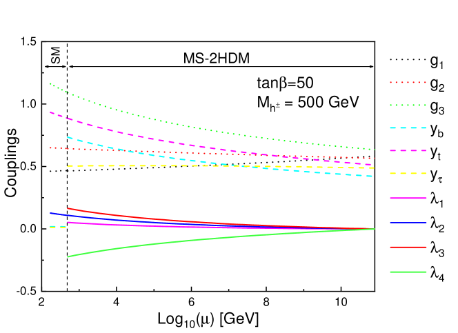
Figure 1: The RG running of the quartic couplings $\lambda_{1,2,3,4}$, gauge and Yukawa couplings from the threshold scale $M_{h^{\pm}}=500$ GeV up to the their first quartic coupling unification scale ${\mu^{(1)}_{X}=10^{11}}$ GeV for $\tan\beta=50$.

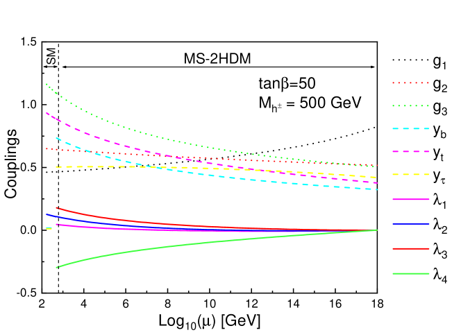
Figure 2: The RG evolution is extended up to the second quartic coupling unification point $\mu^{(2)}_{X}=10^{18}$ GeV.

Figures 1 and 2 exhibit the RG evolution of all relevant couplings of the SM and the MS-2HDM, for $\tan\beta=50$ and $M_{h^{\pm}}=500$ GeV. The vertical dashed line shows the threshold scale $\mu_{\rm thr}=M_{h^{\pm}}=500$ GeV. Visible are at this scale significant discontinuities in the RG running of Yukawa couplings $h_{b}$ and $h_{\tau}$ due to the matching conditions.

In Figure 1, the quartic coupling $\lambda_{2}$, which is correlated to the mass of SM-like Higgs-boson $M_{H}$, decreases at high RG scales due to the evolution of the top-Yukawa coupling $h_{t}$ and turns negative just above the quartic coupling unification scale $\mu_{X}\sim 10^{11}$ GeV, where all quartic couplings vanish. Thereby, for energy scales above the RG scale $\mu_{X}$, we envisage that the MS-2HDM will need to be embedded into another UV-complete theory. Nevertheless, according to our estimates in [32], we have checked that the resulting MS-2HDM potential leads to a metastable but sufficiently long-lived EW vacuum, whose lifetime is many orders of magnitude larger than the age of our Universe. In this respect, we regard the usual constraints derived from convexity conditions on 2HDM potentials [38] to be over-restrictive and unnecessary for our theoretical framework.

Of equal importance is a second conformally-invariant unification point at energy scales close to the reduced Planck mass $\mu^{(2)}_{X}\sim 10^{18}$ GeV, as shown in Figure 2. In this case, the key quartic coupling $\lambda_{2}$ increases and turns positive again. Therefore, in this class of settings, any embedding of the MS-2HDM into a UV-complete theory must have to take quantum gravity into account as well.

By analogy, Figure 3 shows all conformally-invariant quartic coupling unification points in the $(\tan\beta,\,\log_{10}\mu)$ plane, by taking into account different values of threshold scales $\mu_{\rm thr}$, i.e. for $\mu_{\rm thr}\,=\,M_{h^{\pm}}=500\,\text{GeV},\,1\,\text{TeV},\,10\,\text{TeV}\,\text{and}\,100\,\text{TeV}$. The lower curves (dashed curves) correspond to sets of low-scale quartic coupling unification points, while the upper curves (solid curves) give the corresponding sets of high-scale unification points. From Figure 3, we may also observe the domains in which the $\lambda_{2}$ coupling becomes negative. These are given by the vertical $\mu$-intervals bounded by the lower and the upper curves, for a given choice of $M_{h^{\pm}}$ and $\tan\beta$. Evidently, as the threshold scale $\mu_{\rm thr}=M_{h^{\pm}}$ increases, the size of the negative $\lambda_{2}$ domain increases and becomes more pronounced for smaller values of $\tan\beta$.

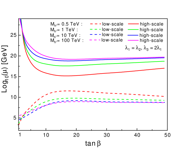
Figure 3: Sets of quartic coupling unification points in the $(\tan\beta,\,\log_{10}\mu)$ plane, for various values of charged Higgs-boson masses $\,M_{h^{\pm}}=500\,\textit{GeV},\,1\,\textit{TeV},\,10\,\textit{TeV}\,\textit{and}\,100\,\textit{TeV}$. The dashed and solid curves show the sets of low-scale $\mu^{(1)}_{X}$ and high-scale $\mu^{(2)}_{X}$ quartic coupling unification points.

Having gained valuable insight from this model, it is important to highlight that the MS-2HDM requires only three additional input parameters: (i) the soft SO$(5)$-breaking mass parameter $m^{2}_{12}$ (or $M_{h^{\pm}})$, (ii) the ratio of VEVs $\tan\beta$, and (iii) the conformally-invariant quartic coupling unification scale $\mu_{X}$ which can only assume two discrete values: $\mu^{(1)}_{X}$ and $\mu^{(2)}_{X}$. Knowing these parameters, the entire Higgs sector of the model can be determined. In the next part, we will give typical predictions in terms of these three input parameters.

4.2 Misalignment Predictions for Higgs Boson Couplings

As was discussed in Section 2, the misalignment of the SM-like Higgs-boson couplings $HVV$ (with $V=W^{\pm},\,Z$), $Ht\bar{t}\,\text{and}\,Hb\bar{b}$ are controlled by the light-to-heavy scalar-mixing parameter $\theta_{\mathcal{S}}$. Obviously, at the quartic coupling unification scale $\mu_{X}$, the SO$(5)$ symmetry of the MS-2HDM is fully restored and this mixing parameter vanishes. However, RG effects induced by the U(1)_Y gauge coupling and the Yukawa couplings break sizeably the SO$(5)$ symmetry, giving rise to a calculable non-zero value for $\theta_{\mathcal{S}}$ and thereby to misalignment predictions for all $H$-boson couplings to SM particles. Here, we present numerical estimates of the predicted deviations of the SM-like Higgs-boson couplings $HVV$ (with $V=W^{\pm},\,Z$), $Ht\bar{t}\,\text{and}\,Hb\bar{b}$, from their respective SM values.

The dependence of the physical misalignment parameter $|1-g^{2}_{HVV}|$ (with $g_{H_{\text{SM}}VV}=1$) as functions of the RG scale $\mu$ is shown in Figure 4. This is given for typical values of $\tan\beta$, such as $\tan\beta=2,\ 5,\,20,\,35\,\text{and}\,50$. As expected, the normalised coupling $g_{HVV}$ approaches the SM value $g_{H_{\text{SM}}VV}=1$ at the lower- and higher-scale quartic coupling unification points, $\mu^{(1)}_{X}$ and $\mu^{(2)}_{X}$, as shown in left and right panels, respectively. We use dashed lines to display our predictions to leading order in $\theta_{\mathcal{S}}$ expansion, while solid lines stand for the exact all-orders result. Since there is a small deviation (below the per-mile level) of $g_{HVV}$ from the SM value, the approximate and exact predicted values are predominately overlapping. Evidently, the misalignment reaches its maximum value for low values of $\tan\beta$ and for the higher quartic coupling unification points.

By analogy, Figures 5 and 6 display misalignment predictions for the $H$-boson couplings to top- and bottom-quarks, for $\tan\beta=2,\ 5,\,20,\,35$ and $50$ and for lower- and higher-scale quartic coupling unification points, respectively. As before, the deviation of the normalised couplings $g_{Htt}$ and $g_{Hbb}$ from their SM values are larger for low values of $\tan\beta$, e.g. $\tan\beta=2$, and for higher-scale quartic coupling unification points $\mu^{(2)}_{X}$. This effect is more noticeable for $g_{Hbb}$, as the amount of misalignment might be even larger than $10\%$. In this case, a comparison between solid and dashed lines shows the appropriateness of our seesaw-inspired approximation in terms of $\theta_{\mathcal{S}}$ parameter.

Last but not least, we confront our misalignment predictions for the SM-like Higgs boson couplings, $g_{HZZ}$, $g_{Htt}$ and $g_{Hbb}$ with existing experimental data from ATLAS and CMS, including their statistical and systematic uncertainties [55]. Our predictions for $\tan\beta=2,\,20,\,35\,\text{and}\,50$ and $M_{h^{\pm}}=500$ GeV are presented in Table 2. The observed results for $g_{HZZ}$ and $g_{Htt}$ are in excellent consistency with the SM and the MS-2HDM. Instead, the LHC data for $g_{Hbb}$ can be fitted to the SM at the $3\sigma$ uncertainty level. Interestingly, the uncertainty level reduces only to $2\sigma$ in the case of MS-2HDM, for $\tan\beta=2$ assuming a high-scale quartic coupling unification scenario. Future precision collider experiments might be able to probe such a scenario.

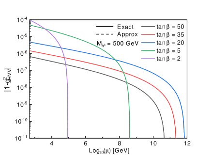
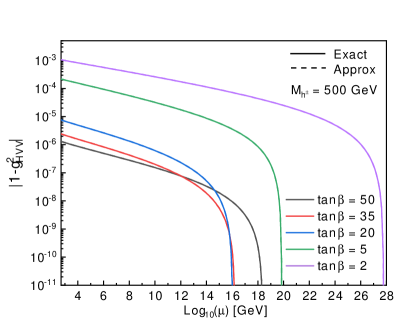
Figure 4: Numerical estimates of the misalignment parameter $|1-g^{2}_{HVV}|$ pertinent to the $HVV$-coupling (with $V=W^{\pm},Z$) as functions of the RG scale $\mu$, for low-scale (left panel) and high-scale (right panel) quartic coupling unification scenarios, assuming $M_{h^{\pm}}=500$ GeV and $\tan\beta=2,\ 5,\,20,\,35$ and $50$.

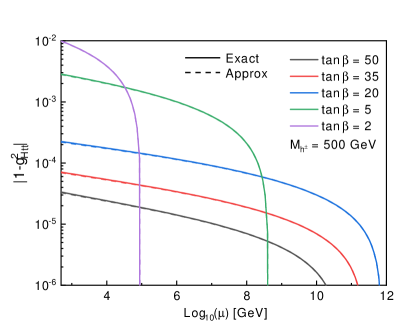
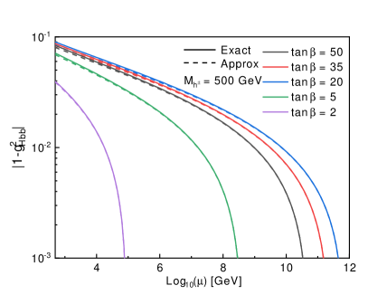
Figure 5: Numerical estimates of the misalignment parameters $|1-g^{2}_{Htt}|$ (left panel) and $|1-g^{2}_{Hbb}|$ (right panel) versus the RG scale $\mu$, for a low-scale quartic coupling unification scenario, assuming $M_{h^{\pm}}=500$ GeV and $\tan\beta=2,\ 5,\,20,\,35$ and $50$.

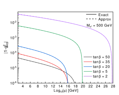
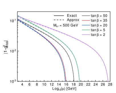
Figure 6: The same as in Figure 5, but for a high-scale quartic coupling unification scenario.

Couplings		ATLAS		CMS		$t_{\beta}=2$		$t_{\beta}=5$		$t_{\beta}=20$		$t_{\beta}=50$
$|g_{HZZ}^{\mu_{X}^{(1)}}|$		[0.86, 1.00]		[0.90, 1.00]		0.999		0.999		0.999		0999
$|g_{HZZ}^{\mu_{X}^{(2)}}|$						0.998		0.999		0.999		0.999
$|g_{Htt}^{\mu_{X}^{(1)}}|$		$1.31^{+0.35}_{-0.33}$		$1.45^{+0.42}_{-0.32}$		1.004		1.001		1.000		1.000
$|g_{Htt}^{\mu_{X}^{(2)}}|$						1.098		1.017		1.000		1.000
$|g_{Hbb}^{\mu_{X}^{(1)}}|$		$0.49^{+0.26}_{-0.19}$		$0.57^{+0.16}_{-0.16}$		0.980		0.964		0.956		0.959
$|g_{Hbb}^{\mu_{X}^{(2)}}|$						0.881		0.926		0.944		0.942

Table 2: Predicted values of the SM-like Higgs boson couplings to the $Z$ boson and to top- and bottom-quarks in the MS-2HDM for both scenarios with low- and high-scale quartic coupling unification, assuming $M_{h^{\pm}}=500$ GeV. The corresponding central values for these couplings from ATLAS and CMS are also given, including their uncertainties [55].

5 Conclusions

The potential of $n$-Higgs Doublet Models ($n$HDMs), with $n\geq 2$ Higgs doublets contains a large number of SU(2)_L-preserving accidental symmetries as subgroups of the symplectic group Sp(2$n)$. We have identified the complete set of maximal continuous symmetries for the so-called SM alignment that may take place in the $n$HDM potentials. These symmetries are necessary for natural SM alignment, without decoupling of large mass scales or fine-tuning. For instance, for the 2HDM, these symmetries ensure alignment for any value of $\tan\beta$ and any form of soft-breaking by bilinear mass terms of the scalar potential. In general, the Maximal Symmetric $n$HDM (MS-$n$HDM) can provide natural SM alignment exhibiting quartic coupling unification up to the Planck scale.

For our illustrations, we have analyzed the simplest realisations of a Type-II 2HDM, the so-called Maximally Symmetric Two-Higgs Doublet Model (MS-2HDM). The scalar potential of this model is determined by a single mass parameter and a single quartic coupling. This minimal form of the potential can be reinforced by an accidental SO$(5)$ symmetry in the bilinear field space, which is isomorphic to Sp(4) in the field basis $\bm{\Phi}$ given in (3). The MS-2HDM can naturally realise the SM alignment limit, in which all SM-like Higgs boson couplings to the EW gauge bosons and to all fermions are equal to their SM strength independently of the values of $\tan\beta$ and $M_{h^{\pm}}$.

The SO$(5)$ symmetry of the MS-2HDM is broken explicitly by RGE effects due to the non-zero U(1)_Y gauge coupling and equally sizeably by the Yukawa couplings. For phenomenological reasons, we have also added a soft SO$(5)$-breaking mass parameter $m^{2}_{12}$ to the scalar potential, which lifts the masses of all pseudo-Goldstone bosons $h^{\pm}$, $h$ and $a$ in the ranges above 500-GeV, consistent with $B$-meson constraints.

To evaluate the RG running of the quartic couplings and the relevant SM couplings, we have employed two-loop 2HDM RGEs from the unification scale $\mu_{X}$ up to charged Higgs-boson mass $M_{h^{\pm}}$. At the RG scale $M_{h^{\pm}}$, we have implemented matching conditions between the MS-2HDM and the SM parameters.

Improving upon an earlier study [8], we have now clearly demonstrated that in the MS-2HDM all quartic couplings can unify at much larger RG scales $\mu_{X}$, where $\mu_{X}$ lies between $\mu^{(1)}_{X}\sim 10^{11}\,$ GeV and $\mu^{(2)}_{X}\sim 10^{20}\,$ GeV. In particular, we have shown that quartic coupling unification can take place in two different conformally invariant points, at which all quartic couplings vanish. This property is unique for this model and can happen at different threshold scales $\mu_{\rm thr}\,=\,M_{h^{\pm}}=500\,\text{GeV},\,1\,\text{TeV},\,10\,\text{TeV}\,\text{and}\,100\,\text{TeV}$. More precisely, the low-scale (high-scale) unification point arises when $\lambda_{2}$ crosses zero and becomes negative (positive) at the RG scale $\mu_{X}^{(1)}$ ($\mu_{X}^{(2)}$). Between these two RG scales, i.e. for $\mu^{(1)}_{X}<\mu<\mu^{(2)}_{X}$, the running quartic coupling $\lambda_{2}(\mu)$ turns negative, which gives rise to a deeper minimum in the effective MS-2HDM potential, whose lifetime is extremely large much larger than the age of our Universe [32].

In summary, the MS-2HDM is a very predictive extension of the SM, as it is governed by two additional parameters: (i) the charged Higgs-boson mass $M_{h^{\pm}}$ (or $m^{2}_{12}$) and (ii) the ratio of VEVs $\tan\beta$. Moreover, requiring conformally-invariant quartic coupling unification at scale $\mu_{X}$, we find to two discrete values for $\mu_{X}$, $\mu^{(1)}_{X}$ and $\mu^{(2)}_{X}$, as functions of $M_{h^{\pm}}$ and $\tan\beta$. Once the values of these theoretical parameters are known, the entire Higgs sector of the model can be determined. In this context, upon the fact that the RG effects sizeably break the SO$(5)$ symmetry, we obtained a calculable non-zero value for the light-to-heavy scalar-mixing parameter $\theta_{\mathcal{S}}$. Thereby, we have been able to present illustrative predictions of misalignment for the SM-like Higgs-boson couplings to the $W^{\pm}$ and $Z$ bosons and to the top- and bottom-quarks. The predicted deviations to $Hb\bar{b}$-coupling is of order $10\%$ and may be observable at future $e^{+}e^{-}$ colliders.

References

• [1] ATLAS Collaboration, ATLAS-CONF-2019-004.
• [2] CMS Collaboration, CMS-PAS-SMP-19-001.
• [3] N. Darvishi, M. Masouminia and K. Ostrolenk, Phys. Rev. D 101 (2020) no.1, 014007 [arXiv:1909.13862 [hep-ph]].
• [4] I. F. Ginzburg, M. Krawczyk and P. Osland, hep-ph/9909455.
• [5] P. H. Chankowski, T. Farris, B. Grzadkowski, J. F. Gunion, J. Kalinowski and M. Krawczyk, Phys. Lett. B 496 (2000) 195 [hep-ph/0009271].
• [6] A. Delgado, G. Nardini and M. Quiros, JHEP 1307 (2013) 054 [arXiv:1303.0800 [hep-ph]].
• [7] M. Carena, I. Low, N. R. Shah and C. E. M. Wagner, JHEP 1404 (2014) 015 [arXiv:1310.2248 [hep-ph]].
• [8] P. S. Bhupal Dev and A. Pilaftsis, JHEP 1412 (2014) 024 Erratum: [JHEP 1511 (2015) 147] [arXiv:1408.3405 [hep-ph]].
• [9] J. Bernon, J. F. Gunion, H. E. Haber, Y. Jiang and S. Kraml, Phys. Rev. D 92 (2015) no.7, 075004 [arXiv:1507.00933 [hep-ph]].
• [10] N.Darvishi and M.Krawczyk, Nucl. Phys. B 926 (2018) 167 [arXiv:1709.07219 [hep-ph]].
• [11] K. Benakli, M. D. Goodsell and S. L. Williamson, Eur. Phys. J. C 78 (2018) 658 [arXiv:1801.08849 [hep-ph]].
• [12] K. Lane and W. Shepherd, Phys. Rev. D 99 (2019) no.5, 055015 [arXiv:1808.07927 [hep-ph]].
• [13] M. Gell-Mann and M. Levy, Nuovo Cim.  16 (1960) 705.
• [14] N. Cabibbo, Phys. Rev. Lett.  10 (1963) 531.
• [15] M.  Kobayashi and T. Maskawa (1973) Prog.Theor.Phys. 49 652–7.
• [16] S. L. Glashow, J. Iliopoulos and L. Maiani, Phys. Rev. D 2 (1970) 1285.
• [17] E. A. Paschos, Phys. Rev. D 15 (1977) 1966.
• [18] S. L. Glashow and S. Weinberg, Phys. Rev. D 15 (1977) 1958.
• [19] N. Darvishi and A. Pilaftsis, arXiv:1912.00887 [hep-ph].
• [20] H. Georgi and D. V. Nanopoulos, Phys. Lett.  82B (1979) 95.
• [21] J. F. Gunion and H. E. Haber, Phys. Rev. D 67 (2003) 075019 [hep-ph/0207010].
• [22] I. F. Ginzburg and M. Krawczyk, Phys. Rev. D 72 (2005) 115013 [hep-ph/0408011].
• [23] H. E. Haber and O. Stål, Eur. Phys. J. C 75 (2015) no.10, 491 Erratum: [Eur. Phys. J. C 76 (2016) no.6, 312] [arXiv:1507.04281 [hep-ph]].
• [24] B. Grzadkowski, H. E. Haber, O. M. Ogreid and P. Osland, JHEP 1812, 056 (2018) [arXiv:1808.01472 [hep-ph]].
• [25] T. D. Lee, Phys. Rev. D 8 (1973) 1226.
• [26] G. C. Branco, P. M. Ferreira, L. Lavoura, M. N. Rebelo, M. Sher and J. P. Silva, Phys. Rept.  516 (2012) 1 [arXiv:1106.0034 [hep-ph]].
• [27] A. Arbey, F. Mahmoudi, O. Stal and T. Stefaniak, Eur. Phys. J. C 78 (2018) 182 [arXiv:1706.07414 [hep-ph]].
• [28] E. Hanson, W. Klemm, R. Naranjo, Y. Peters and A. Pilaftsis, arXiv:1812.04713 [hep-ph].
• [29] A. Pilaftsis, Phys. Lett. B 706 (2012) 465 [arXiv:1109.3787 [hep-ph]].
• [30] A. Pilaftsis, Phys. Rev. D 93 (2016) no.7, 075012 [arXiv:1602.02017 [hep-ph]].
• [31] P. S. Bhupal Dev and A. Pilaftsis, J. Phys. Conf. Ser.  873 (2017) no.1, 012008 [arXiv:1703.05730 [hep-ph]].
• [32] N. Darvishi and A. Pilaftsis, Phys. Rev. D 99 (2019) no.11, 115014 [arXiv:1904.06723 [hep-ph]].
• [33] A. Pilaftsis and C. E. M. Wagner, Nucl. Phys. B 553 (1999) 3 doi:10.1016/S0550-3213(99)00261-8 [hep-ph/9902371].
• [34] ATLAS Collaboration, Phys. Lett. B 716 (2012) 1 [arXiv:1207.7214 [hep-ex]].
• [35] CMS Collaboration, Phys. Lett. B 716 (2012) 30 [arXiv:1207.7235 [hep-ex]].
• [36] P. Minkowski, Phys. Lett.  67B (1977) 421;
T. Yanagida, Prog. Theor. Phys.  64 (1980) 1103;
R. N. Mohapatra and G. Senjanovic, Phys. Rev. Lett.  44 (1980) 912;
J. Schechter and J. W. F. Valle, Phys. Rev. D 22 (1980) 2227.
• [37] F. J. Botella and J. P. Silva, Phys. Rev. D 51 (1995) 3870 [hep-ph/9411288].
• [38] N. G. Deshpande and E. Ma, Phys. Rev. D 18 (1978) 2574.
• [39] M. Maniatis, A. von Manteuffel, O. Nachtmann and F. Nagel, Eur. Phys. J. C 48 (2006) 805 [hep-ph/0605184].
• [40] C. C. Nishi, Phys. Rev. D 74 (2006) 036003 Erratum: [Phys. Rev. D 76 (2007) 119901] [hep-ph/0605153].
• [41] I. P. Ivanov, Phys. Rev. D 75 (2007) 035001 Erratum: [Phys. Rev. D 76 (2007) 039902] [hep-ph/0609018].
• [42] R. A. Battye, G. D. Brawn and A. Pilaftsis, JHEP 1108 (2011) 020 [arXiv:1106.3482 [hep-ph]].
• [43] J. Goldstone, Nuovo Cim.  19 (1961) 154.
• [44] K. A. Olive et al. [Particle Data Group], Chin. Phys. C 38 (2014) 090001.
• [45] R. D. Peccei and H. R. Quinn, Phys. Rev. Lett.  38 (1977) 1440.
• [46] S. Weinberg, Phys. Rev. Lett.  40 (1978) 223.
• [47] F. Wilczek, Phys. Rev. Lett.  40 (1978) 279.
• [48] M. Misiak and M. Steinhauser, Eur. Phys. J. C 77 (2017) no.3, 201 [arXiv:1702.04571 [hep-ph]].
• [49] J. Oredsson and J. Rathsman, arXiv:1810.02588 [hep-ph].
• [50] D. Chowdhury and O. Eberhardt, JHEP 1511, 052 (2015) [arXiv:1503.08216 [hep-ph]].
• [51] M. E. Krauss, T. Opferkuch and F. Staub, Eur. Phys. J. C 78 (2018) 1020 [arXiv:1807.07581 [hep-ph]].
• [52] A. V. Bednyakov, JHEP 1811 (2018) 154 doi:10.1007/JHEP11(2018)154 [arXiv:1809.04527 [hep-ph]].
• [53] F. Staub, Comput. Phys. Commun.  185 (2014) 1773 [arXiv:1309.7223 [hep-ph]].
• [54] M. Carena, J. Ellis, J. S. Lee, A. Pilaftsis and C. E. M. Wagner, JHEP 1602 (2016) 123 [arXiv:1512.00437 [hep-ph]].
• [55] G. Aad et al. [ATLAS and CMS Collaborations], JHEP 1608 (2016) 045 [arXiv:1606.02266 [hep-ex]].
• [56] C. C. Nishi, Phys. Rev. D 83 (2011) 095005 [arXiv:1103.0252 [hep-ph]].
• [57] B. Grinstein and P. Uttayarat, JHEP 1306 (2013) 094 Erratum: [JHEP 1309 (2013) 110] [arXiv:1304.0028 [hep-ph]].
• [58] J. Baglio, O. Eberhardt, U. Nierste and M. Wiebusch, Phys. Rev. D 90 (2014) no.1, 015008 [arXiv:1403.1264 [hep-ph]].
• [59] D. Buttazzo, G. Degrassi, P. P. Giardino, G. F. Giudice, F. Sala, A. Salvio and A. Strumia, JHEP 1312 (2013) 089 [arXiv:1307.3536 [hep-ph]].
• [60] L. J. Hall and M. B. Wise, Nucl. Phys. B 187 (1981) 397.
• [61] V. D. Barger, J. L. Hewett and R. J. N. Phillips, Phys. Rev. D 41, 3421 (1990).
• [62] A. Pich and P. Tuzon, Phys. Rev. D 80 (2009) 091702 [arXiv:0908.1554 [hep-ph]].