Unusual stationary state in Brownian systems with Lorentz force
Abstract
In systems with overdamped dynamics, the Lorentz force reduces the diffusivity of a Brownian particle in the plane perpendicular to the magnetic field. The anisotropy in diffusion implies that the Fokker-Planck equation for the probabiliy distribution of the particle acquires a tensorial coefficient. The tensor, however, is not a typical diffusion tensor due to the antisymmetric elements which account for the fact that Lorentz force curves the trajectory of a moving charged particle. This gives rise to unusual dynamics with features such as additional Lorentz fluxes and a nontrivial density distribution, unlike a diffusive system. The equilibrium properties are, however, unaffected by the Lorentz force. Here we show that by stochastically resetting the Brownian particle, a nonequilibrium steady state can be created which preserves the hallmark features of dynamics under Lorentz force. We then consider a minimalistic example of spatially inhomogeneous magnetic field, which shows how Lorentz fluxes fundamentally alter the boundary conditions giving rise to an unusual stationary state.
I Introduction
The Lorentz force due to an external magnetic field modifies the trajectory of a charged, moving particle without performing work on it. This results in characteristic helical trajectories in case of a constant magnetic field. Such motion is an idealization which compeletely ignores dissipative effects that are highly relevant in, for instance, plasma physics Goldston and Rutherford (1995). In fact, dissipative effects are dominant in colloidal systems where the dynamics are overdamped. Whereas the effect of Lorentz force in the context of solid-state physics and plasma physics has been throughly studied, much less is known about its effect on diffusion systems subjected to an external magnetic field.
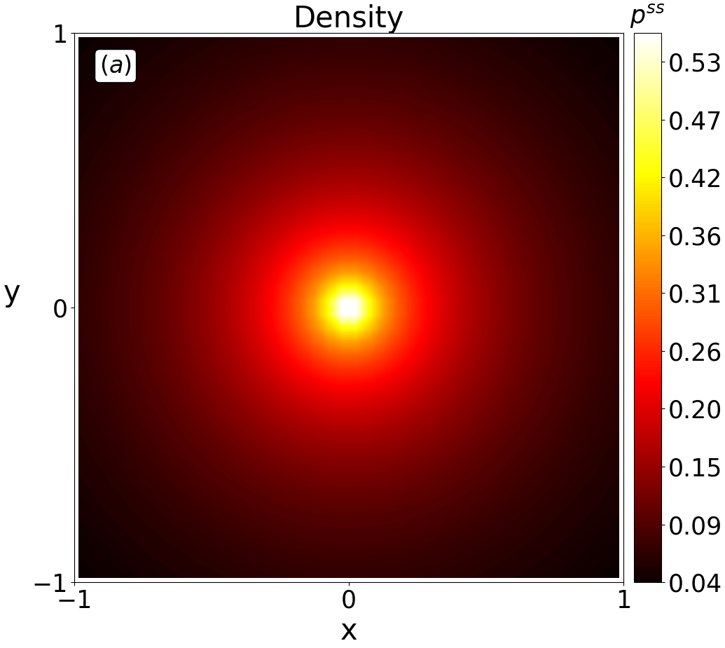
A known consequence of the Lorentz force is a reduction of the diffusion coefficient in the plane perpendicular to the magnetic field, whereas the diffusion along the field is unaffected Balakrishnan (2008); Vuijk et al. (2019a). The anisotropy in diffusion implies that the corresponding Fokker-Planck equation for the probability distribution acquires a tensorial coefficient, the components of which are determined by the applied magnetic field, the temperature, and the friction coefficient. The tensor, however, is not a typical diffusion tensor due to the antisymmetric elements which account for the fact that Lorentz force curves the trajectory of a charged, diffusing particle, giving rise to additional Lorentz fluxes Chun et al. (2018); Vuijk et al. (2019b). We have recently shown that the dynamics under this tensor are fundamentally different from purely diffusive Abdoli et al. (2020). In particular, the nonequilibrium dynamics are characerized by features such as additional Lorentz fluxes and a nontrivial density distribution [see Fig. 1]. These have implications for dynamical properties of the system such as the mean first-passage time, escape probability, and phase transition dynamics in fluids Vuijk et al. (2019a); Abdoli et al. (2020).
Since the Lorentz force arising from an external magnetic field does no work on the system, the equilibrium properties of the system are unaffected. This implies that to observe the nontrivial effects of Lorentz force, the system must be maintained out of equilibrium, possibly in a nonequilibrium steady state. This can be done by driving the system out of equilibrium, for instance, via a time-dependent external potential or shear. Alternatively, one may consider internally driven systems, a particularly interesting example of which is active matter which is ubiquitous in biology Alvarado et al. (2013, 2017); Tan et al. (2018). We recently demonstrated that a system of active Brownian particles subjected to a spatially inhomogeneous Lorentz force relaxes towards a nonequilibrium steady state with inhomogeneous density distribution and macroscopic fluxes (Vuijk et al., 2020). The distinctive dynamics of a charged, passive, diffusing particle under Lorentz force may be appreciated by noting that if the tensor entering the Fokker-Planck equation was positive symmetric, i.e., a diffusion-like tensor, there would be no fluxes in the steady state.
We take a different approach to drive the system into a nonequilibrium steady state: the particle, while diffusing under the influence of Lorentz force, is stochastically reset to a prescribed location at a constant rate. The concept of stochastic resetting was introduced by Evans and Majumdar Evans and Majumdar (2011a). In their model, a Brownian particle diffuses freely until it is reset to its initial location. The waiting time between two consecutive resetting events is a random variable for which the Poissonian distribution has been widely used. Evans and Majumdar showed that diffusion under stochastic resetting gives rise to a nonequilibrium stationary state with a non-Gaussian position distribution and particle flux. They also demonstrated that the mean first-passage time for this model is finite and has a minimum value at an optimal resetting rate. Over the last few years, stochastic resetting has been applied to a wide variety of random processes Evans and Majumdar (2011b); Pal et al. (2016); Scacchi and Sharma (2018); Gupta (2019); Pal and Prasad (2019) and generalized to include non-Markovian resetting and dependence of resetting on internal dynamics Nagar and Gupta (2016); Eule and Metzger (2016); Bodrova et al. (2019); Falcao and Evans (2017). It has been shown that it gives rise to intriguing phenomena such as dynamical phase transitions (Kusmierz et al., 2014; Majumdar et al., 2015), universal properties which are insensitive to details of underlying random process Reuveni (2016); Pal and Reuveni (2017); Pal et al. (2019) and optimal search strategies Kuśmierz and Gudowska-Nowak (2015).
In this paper, we show that under stochastic resetting a Brownian system settles into an unusual stationary state which preserves the hallmark features of dynamics under Lorentz force. In the case of a constant magnetic field, the nonequilibrium steady state is characterized by a non-Gaussian probability density, diffusive and Lorentz fluxes. These Lorentz fluxes reflect the behavior shown in Fig. 1 and are reminiscent of Brownian vortices in a system of colloidal particles diffusing in an optical trap Roichman et al. (2008); Sun et al. (2009, 2010). Due to the Lorentz force, the flux is not along the density gradient. This holds even for a constant tensorial coefficient. As a consequence, the boundary conditions for diffusion in finite or semi-finite domains take a form different from the typical Neumann or Dirichlet conditions. By considering a minimalistic example, we show how the modified boundary condition gives rise to un unusual stationary state with no counterpart in purely diffusive systems.
The paper is organized as follows. In Sec. II, we provide a brief theoretical description of diffusion under Lorentz force and stochastic resetting. In Sec. III, we derive the steady-state solution to the governing Fokker-Planck equation for constant and inhomogeneous magnetic fields. Finally, we discuss our results and present an outlook in section IV.
II Theory and Simulation
We consider a single diffusing particle which is stochastically reset to its initial position at a constant rate . The particle is subjected to Lorentz force arising from an external magnetic field where indicates the direction of the magnetic field and is the magnitude. Our theoretical approach is based on the Fokker-Planck equation for the position distribution of the particle. For a spatially inhomogeneous magnetic field, the probability for finding the particle at position at time , given that it started at , obeys the following Fokker-Planck equation Evans and Majumdar (2011a); Vuijk et al. (2019b); Chun et al. (2018)
| (1) | ||||
where stands for derivative with respect to and the tensor is
| (2) |
where is the diffusion coefficient of a freely diffusing particle and quantifies the strength of Lorentz force relative to frictional force Vuijk et al. (2020). Here is the friction coefficient, is the Boltzmann constant, is the temperature and is the charge of the particle. The matrix is defined by . and are the symmetric and antisymmetric parts of the tensor .
Note that Eq.(1) is not of the form of a continuity equation. The first term on the right hand side of Eq. (1) represents the contribution from overdamped motion under Lorentz force. The second and third terms stand for the contribution due to the resetting of the particle: the second term represents the loss of the probability from the position owing to resetting to the initial position while the third term stands for the gain of probability at due to resetting from all other positions. The flux in the system is given as
| (3) |
which can be decomposed into the diffusive flux
| (4) |
and the Lorentz flux
| (5) |
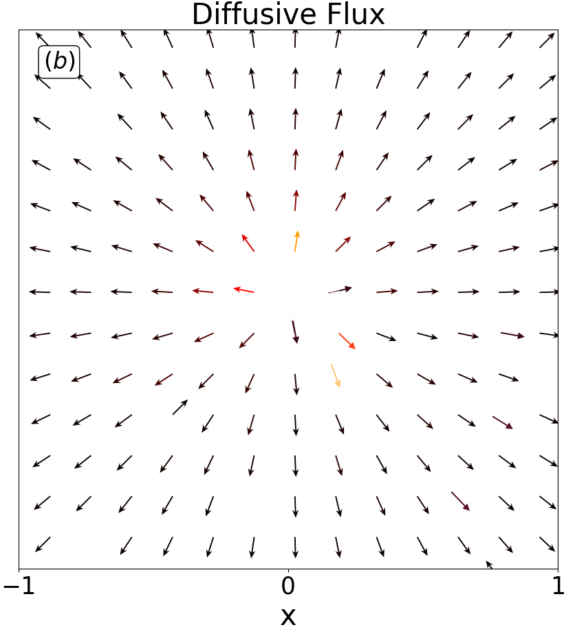
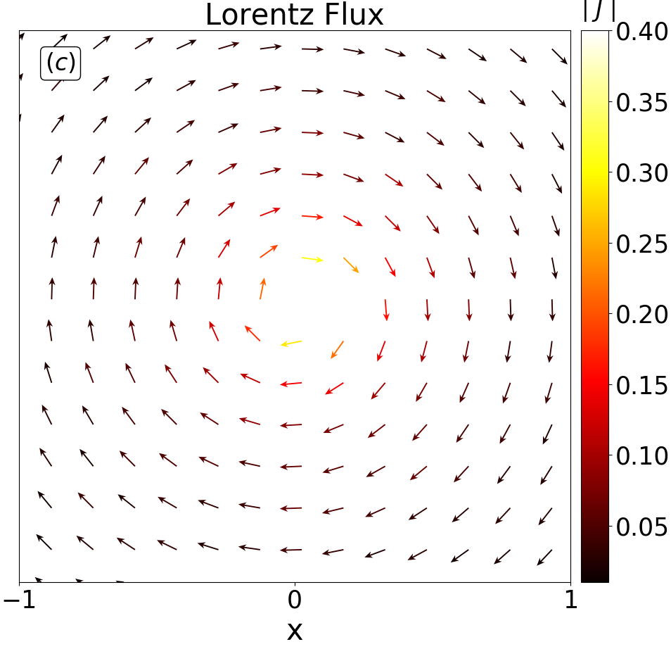
Note that the diffusive flux does not depend on the sign of the magnetic field. In contrast, the Lorentz flux can be reversed by reversing the magnetic field. Moreover, it is always perpendicular to the diffusive flux. These properties of Lorentz flux, which are straightforward consequences of how the Lorentz force affects a particle’s trajectory, constitute the main rationale behind the above decomposition. Although the dynamics are overdamped it is the presence of these Lorentz fluxes which makes the dynamics under Lorentz force distinct from a purely diffusive system in which only diffusive fluxes exist.
In order to confirm our analytical predictions, Brownian dynamics simulations are performed using the Langevin equation of motion Langevin (1908). It has been shown that the overdamped Langevin equation for a Brownian motion in a magnetic field can yield unphysical values for velocity-dependent variables like flux (Vuijk et al., 2019b). Therefore, we use the underdamped Langevin equation with a sufficiently small mass. Omitting hydrodynamics, the dynamics of the particle are described by the following Langevin equations Vuijk et al. (2019b); Abdoli et al. (2020):
| (6) |
where is the mass of the particle and is Gaussian white noise with zero mean and time correlation . The waiting time between two consecutive resetting events is a random variable with Poisson distribution: in a small time interval the particle is either reset to its initial position with probability or continues to diffuse with probability . Throughout the paper we fix the mass to and the integration time step to where is the time for diffusion over one unit distance. In fact, it has been shown that even with a mass the trajectory of the particle from Eq. (6) converges on the trajectory from the small-mass limit of this equation Vuijk et al. (2019b). However, to ensure that the dynamics are overdamped, we have performed simulations with even a smaller mass. The simulation results did not show any significant change. Since the magnetic field is applied in the direction, the Lorentz force has no effect on the motion in this direction. As a consequence, we restrict our analysis to the motion in the plane. Accordingly, the vector denotes the coordinates of the particle and the tensorial coefficient is a matrix.
III Nonequilibrium steady state
In this section, we determine the steady-state solution to the Eq. (1), first for a constant magnetic field and then for a special choice of spatially inhomogeneous field.
III.1 Constant magnetic field
In the case of a constant magnetic field , it can be easily shown that . This implies that the tensor in Eq. (1) can be replaced by which yields the following Fokker-Planck equation:
| (7) | ||||
The steady-state solution of this equation is obtained by setting which, in two dimensions, can be written as Evans and Majumdar (2011a)
| (8) |
where is the modified Bessel function of the second kind of order zero and . Using Eqs (3) and (8) the diffusive flux can be written as
| (9) |
where is the modified Bessel function of the second kind of order one, is the distance from the starting point of the particle and is a unit vector in the radial direction.
The steady-state solution in case of a constant magnetic field is the same as obtained in Ref. Evans and Majumdar (2011a, 2014) with trivial rescaling of the diffusion coefficient wherein for a freely diffusing particle is replaced by for diffusion under Lorentz force. The distinctive new feature of the steady state is the presence of additional Lorentz fluxes, which can be written as
| (10) |
where is a unit vector in the azimuthal direction. On comparing Eqs. (10) and (9), it is evident that the Lorentz flux is nothing else but diffusive flux deflected by the applied magnetic field.
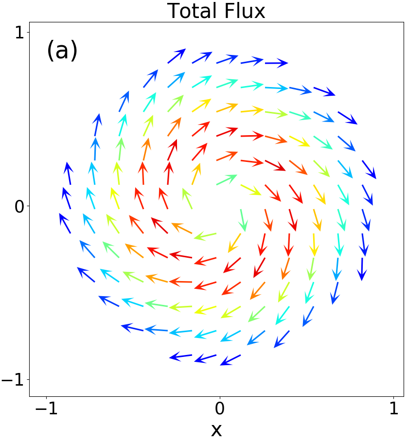
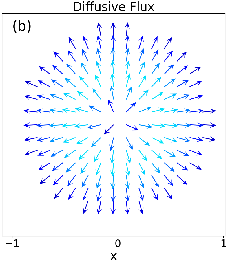
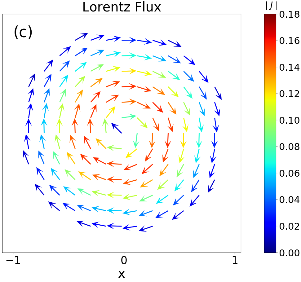
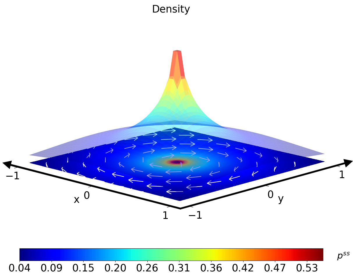
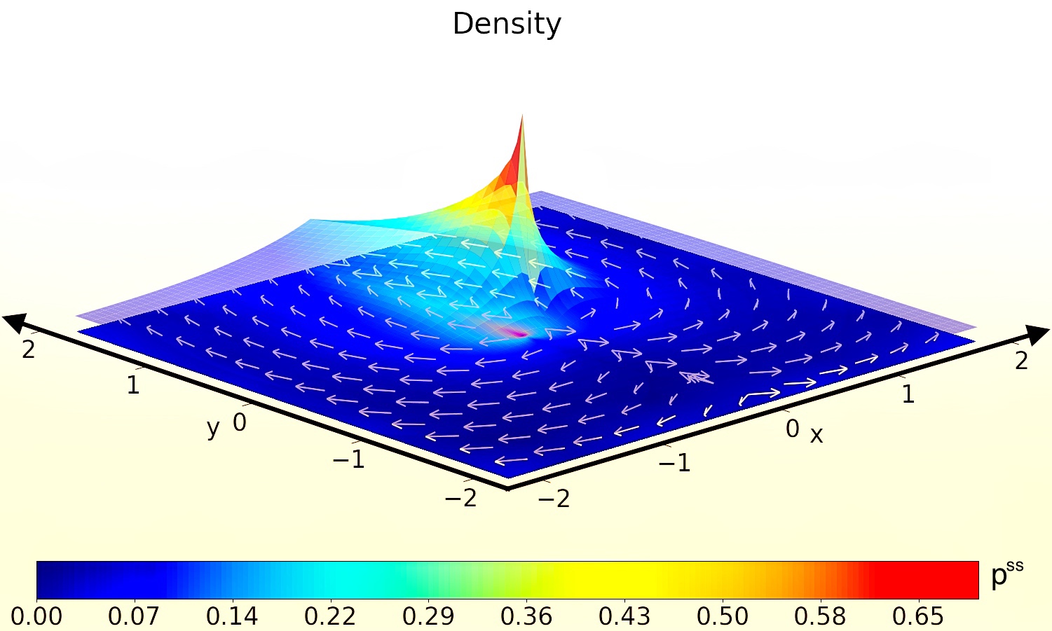
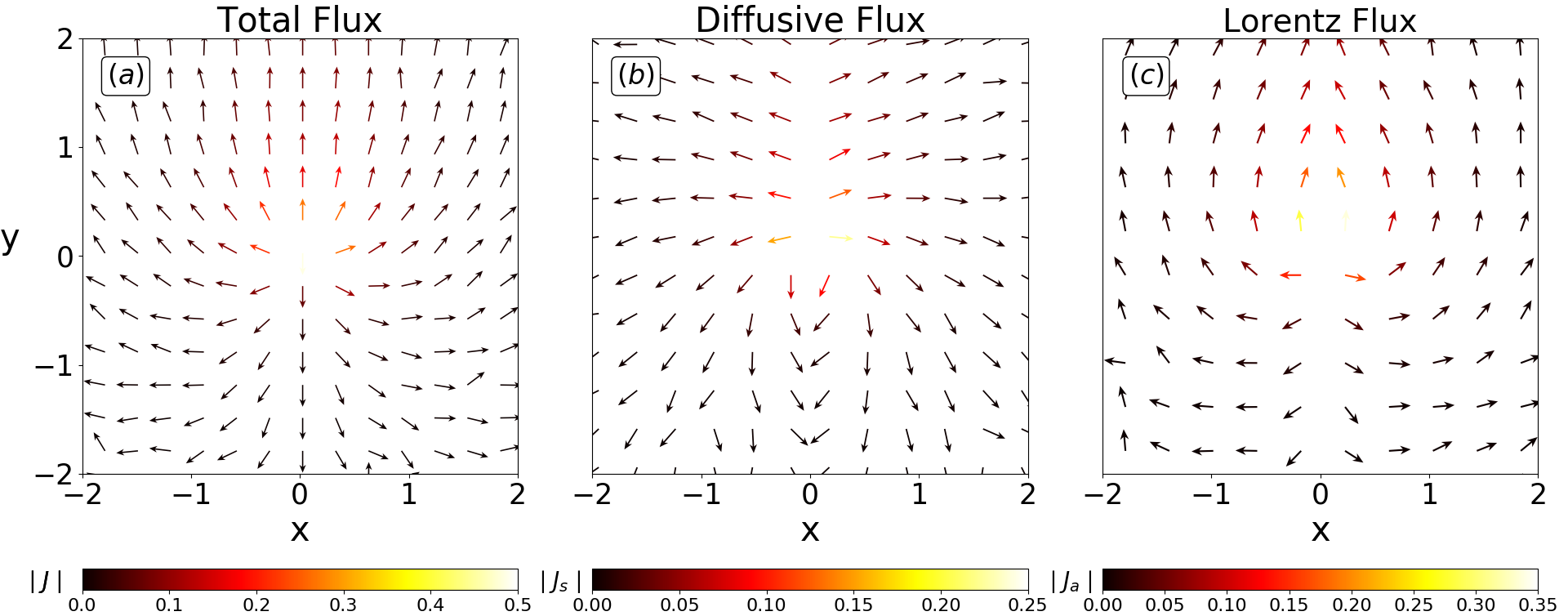
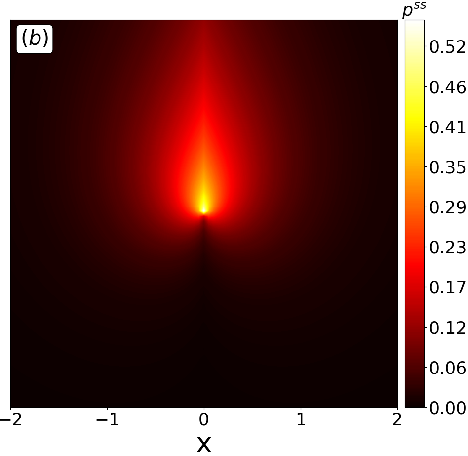
In Fig. 2 we show a surface plot together with a contour plot of the probability density in the stationary state of the system from Eq. (8). The applied magnetic field is such that . The particle is stochastically reset to its initial position at a constant rate . Lorentz fluxes (Eq. (10)) are shown as white arrows on top of the contour plot. These fluxes resemble Brownian vortex observed in a system of colloidal particle diffusing in an optical trap Roichman et al. (2008); Sun et al. (2009, 2010). Figures 3(a) to 3(c) show, respectively, the results for the probability density, diffusive fluxes, and the Brownian vortices in the stationary state of the system, obtained from Brownian dynamics simulations. These results are in excellent agreement with the theoretical results shown in Fig. 2.
III.2 Spatially inhomogeneous magnetic field: a minimal example
As shown above, Lorentz fluxes in the steady state result from deflection of the radial fluxes. In fact, for a constant magnetic field, they do not affect the relaxation dynamics Abdoli et al. (2020). This is no longer the case when the magnetic field is inhomogeneous; the steady-state solution, as we show below, is determined by the diffusive and Lorentz fluxes.
We consider a minimalistic example of a spatially inhomogeneous magnetic field to highlight how the Lorentz fluxes fundamentally alter the boundary conditions giving rise to an unusual stationary state. The system is divided into two half-planes by the line [see Fig. 4]. Each half plane is subjected to a constant magnetic field with the same magnitude, but opposite direction such that
| (11) |
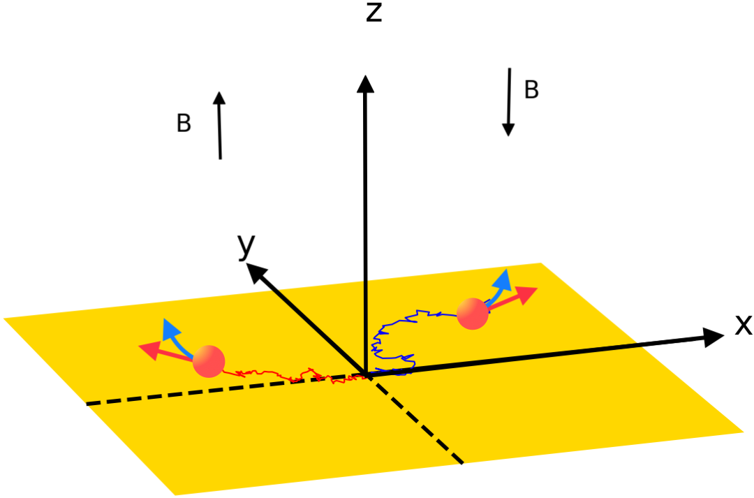
where is a (constant) parameter. In Fig. 4, two different trajectories of the diffusing particle are shown. The red arrows depict the motion of the particle at a given position without Lorentz force, whereas a similar motion in the presence of Lorentz force is shown by blue arrows. As the particle moves away from the origin, the Lorentz force makes the particle undergo a bias toward counterclockwise motion if and clockwise if . This implies that there is no flux across the line .
This particular choice of the magnetic field ensures that the symmetric part of the tensor, , is a constant tensor in the entire plane, whereas the antisymmetric part, , changes sign at . It thus follows that the governing Fokker-Planck equation for the position distribution of the particle is the same as in Sec. III.1 (Eq. (7)) with the boundary condition that the component of the flux (Eq. (3)) is zero at . Since the flux is composed of both diffusive and Lorentz components, the boundary condition reads as
| (12) |
where is an oblique vector, the direction of which is determined by the magnetic field. This boundary condition is known as the oblique boundary condition and is often employed in theory of wave propagation in presence of obstacles (Gilbarg and Trudinger, 2015; Keller et al., 1981). Note that for , this reduces to the ordinary Neumann boundary condition.
The Fokker-Planck equation (7) with the boundary condition in Eq. (12) can be solved using the method of partial Fourier transforms (Hoernig, 2010) [see the appendix for details]. The steady-state solution, obtained for , is given as
| (13) |
where . One can show that for a system without Lorentz force this expression correctly reduces to the (analytical) results obtained by Evans and Majumdar (Evans and Majumdar, 2011a).
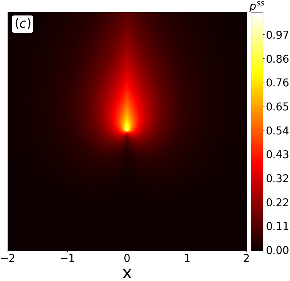
In Fig. 5 we show a surface plot on top of a contour plot of the probability density in the stationary state from Eq. (13). The Lorentz fluxes are shown by white arrows. That an inhomogeneous magnetic field induces an unusual stationary state in the system can be observed by a comparison with Fig. 2.
Figure 6 shows the results from Brownian dynamics simulations with and . The total, diffusive, and Lorentz fluxes in the system are shown in (a-c), respectively. As can be seen in Fig. 6, the component of the total flux is zero at .
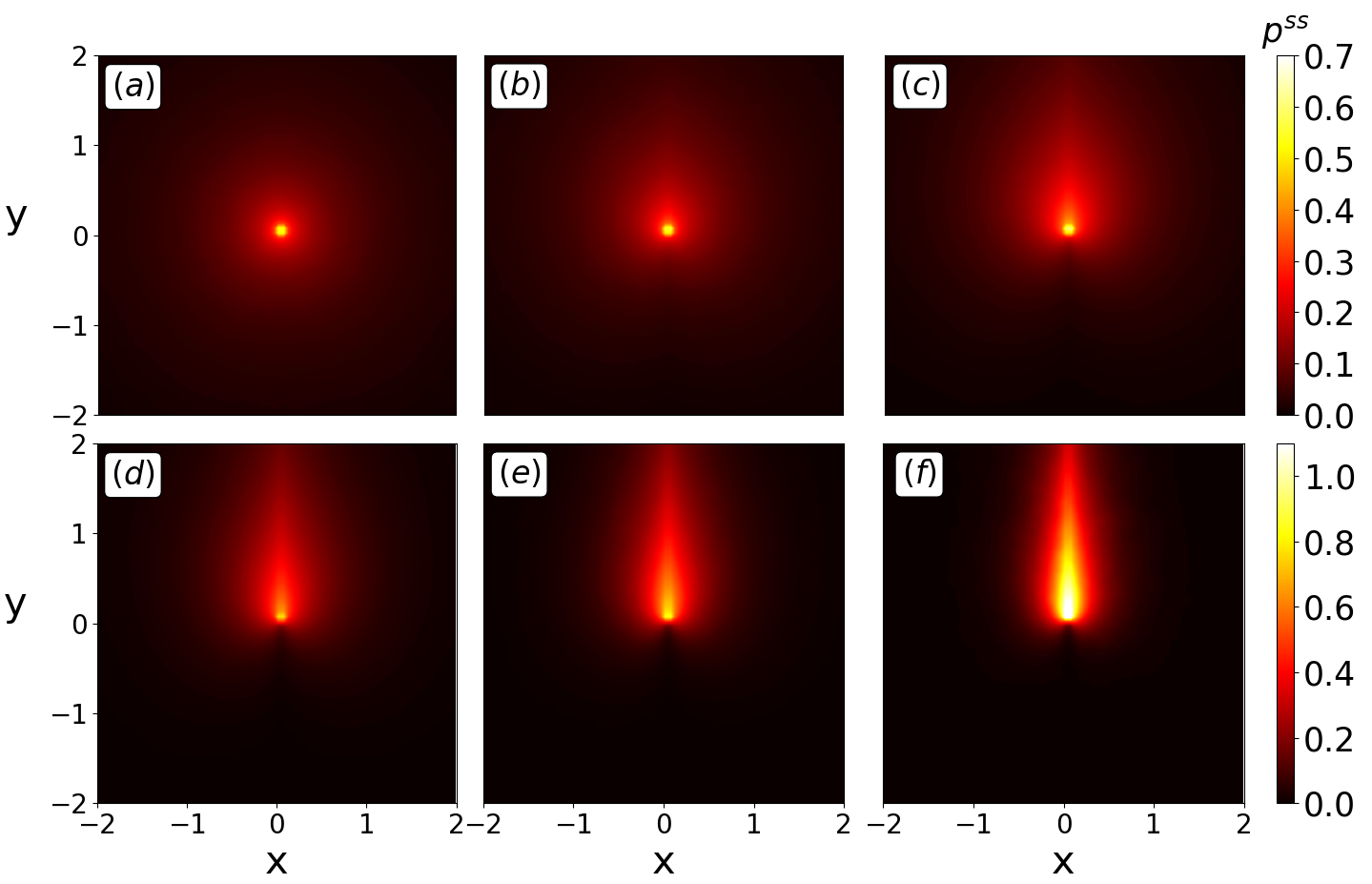
Figure 7 shows the steady-state distribution of the particle’s position, obtained from simulations for different values of . The particle is stochastically reset to its initial position at a constant rate for all values of . As can be seen in Fig. 7, the distribution has a candle-flame-like form which is not symmetric with respect to axis. This can be understood as the accumulation resulting from the equal and opposite Lorentz fluxes at . The distribution becomes increasingly stretched along the direction with increasing magnetic field. A comparison of numerical solutions of Eq. (13) (not shown) with the simulations confirms our analytical predictions.
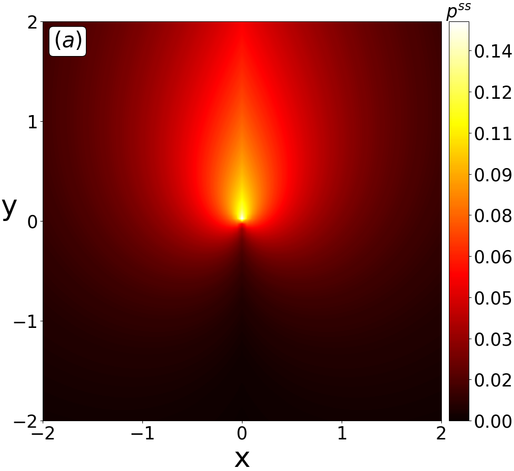
In Fig. 8 we show the steady-state distribution of the position of the particle from simulations for different values of with . The distribution is stretched along the direction. The width of the distribution along direction decreases with increasing .
This minimalistic example shows how Lorentz flux fundamentally alters the probability density and induces an unusual stationary state. Experimentally realizable magnetic fields are likely to have more complicated shapes; however, this does not change the conclusions of this study.
IV Discussion and Conclusion
Lorentz force has the unique property that it depends on the velocity of the particle and is always perpendicular to it. Although this force generates particle currents, they are purely rotational and do no work on the system. As a consequence, the equilibrium properties of a Brownian system, for instance the steady-state density distribution, are independent of the applied magnetic field. The dynamics, however, are affected by Lorentz force: the Fokker-Planck equation picks up a tensorial coefficient, which reflects the anisotropy of the particle’s motion. The diffusion rate perpendicular to the direction of the magnetic field decreases with increasing field whereas the rate along the field remains unaffected. In addition to this effect, Lorentz force gives rise to Lorentz fluxes which result from the deflection of diffusive fluxes Vuijk et al. (2019b); Abdoli et al. (2020).
The effects caused by the Lorentz force, however, occur only in nonequilibrium and cease to exist when the distribution of particles reaches equilibrium. A system subjected to stochastic resetting, in contrast, is continuously driven out of equilibrium. In this paper, we showed that by stochastically resetting the Brownian particle to a prescribed location, a nonequilibrium steady state can be created which preserves the hallmark features of dynamics under Lorentz force : a nontrivial density distribution and Lorentz fluxes. We considered a minimalistic example of spatially inhomogeneous magnetic field, which shows how Lorentz fluxes fundamentally alter the boundary conditions giving rise to an unusual stationary state with no counterpart in (purely) diffusive systems.
One may wonder about the choice of stochastic resetting in this study. Although there are several methods to drive a system into a nonequilibrium steady state, stochastic resetting is unique in the sense that it simply renews the underlying (random) process and therefore, in some sense, preserves the dynamics of the underlying process in the steady state. Contrast this with a system of active Brownian particles subjected to Lorentz force Vuijk et al. (2020) in which Lorentz force couples with the nonequilibrium dynamics of an active particle via its self-propulsion. Although most of the research in stochastic resetting is theoretical, stochastic resetting has been realized experimentally in a system of a colloidal particle which is reset using holographic optical tweezers Tal-Friedman et al. (2020). Resetting also features naturally in the measurement of position-dependent diffusion of a particle diffusing near a wall which experiences inhomogeneous drag due to hydrodynamics. The position-dependent diffusion coefficient is measured by letting the particle diffuse freely from a given initial location for a certain period of time before resetting it, using optical tweezers, to the initial location (Dufresne et al., 2001). From the ‘finite-time’ ensemble of measurements, the diffusion coefficient is obtained from the mean squared displacement.
In this work we focused only on the steady-state properties of the system. The investigation of how Lorentz force affects the mean first-passage time and escape probability in such systems is left for a future study.
Acknowledgments
We would like to acknowledge Holger Merlitz for fruitful discussions and suggestions.
Appendix A Oblique-Derivative Half-Plane Master Equation
Partial differential equations with oblique derivative boundary conditions often arise in the theory of waves, for instance, waves on the ocean or in a rotating plane (Gilbarg and Trudinger, 2015; Keller et al., 1981). There is a vast amount of mathematical literature on this subject. Here we use the method of partial Fourier transforms adopted from Ref. (Hoernig, 2010). We consider as a reflecting boundary, for which the zero flux condition can be written as
| (14) |
where is the oblique vector. We consider a diffusing particle that is stochastically reset to at a constant rate . Later we will set to obtain the solution for our particular case.
The master equation for the stationary probability density is
| (15) |
We define the partial Fourier transform as
| (16) |
and its inverse as
| (17) |
The transformed Fokker-Planck equation [Eq. (15)] becomes
| (18) |
where and . The transformed boundary condition reads as
| (19) |
where is the imaginary unit. The general solution to Eq. (18) is:
| , | (20a) | ||||
| . | (20b) |
The boundary condition that is zero as implies . That the probability density is continuous on implies
| (21) |
Substituting Eq. (20a) into Eq. (19) gives a relationship between and :
| (22) |
Now one can rewrite Eqs. (20a) and (20b) as
| (23) |
where . Using this expression one gets
| (24) |
The second derivative of in Eq. (18) can be replaced by Eq. (A), which results in . After some simplifications one gets
| (25) |
For the system studied in this paper, we set . Thus
| (26) |
We could not find a closed analytical form for the inverse Fourier transform of Eq. (26). Nevertheless, the following intergal can be evaluated numerically to obtain the steady-state solution:
| (27) |
Note the factor on the right hand side of the Eq. (27), which accounts for the (symmetric) extension of the solution to the half-plane. For special case of , it is easy to show that the above integral reduces to
| (28) |
where where is the distance from the origin, same as reported in Ref. (Evans and Majumdar, 2011a) for a two dimensional (symmetric) diffusion under stochastic resetting.
References
- Goldston and Rutherford (1995) Robert J Goldston and Paul Harding Rutherford, Introduction to plasma physics (CRC Press, 1995).
- Balakrishnan (2008) V. Balakrishnan, Elements of Nonequilibrium Statistical Mechanics (Ane Books, 2008).
- Vuijk et al. (2019a) H. D. Vuijk, J. M. Brader, and A. Sharma, Soft matter 15, 1319 (2019a).
- Chun et al. (2018) Hyun-Myung Chun, Xavier Durang, and Jae Dong Noh, “Emergence of nonwhite noise in langevin dynamics with magnetic lorentz force,” Physical Review E 97, 032117 (2018).
- Vuijk et al. (2019b) Hidde Derk Vuijk, Joseph Michael Brader, and Abhinav Sharma, “Anomalous fluxes in overdamped brownian dynamics with lorentz force,” Journal of Statistical Mechanics: Theory and Experiment 2019, 063203 (2019b).
- Abdoli et al. (2020) Iman Abdoli, Hidde Derk Vuijk, Jens-Uwe Sommer, Joseph Michael Brader, and Abhinav Sharma, “Nondiffusive fluxes in a brownian system with lorentz force,” Physical Review E 101, 012120 (2020).
- Alvarado et al. (2013) José Alvarado, Michael Sheinman, Abhinav Sharma, Fred C MacKintosh, and Gijsje H Koenderink, “Molecular motors robustly drive active gels to a critically connected state,” Nature Physics 9, 591–597 (2013).
- Alvarado et al. (2017) José Alvarado, Michael Sheinman, Abhinav Sharma, Fred C MacKintosh, and Gijsje H Koenderink, “Force percolation of contractile active gels,” Soft matter 13, 5624–5644 (2017).
- Tan et al. (2018) Tzer Han Tan, Maya Malik-Garbi, Enas Abu-Shah, Junang Li, Abhinav Sharma, Fred C MacKintosh, Kinneret Keren, Christoph F Schmidt, and Nikta Fakhri, “Self-organized stress patterns drive state transitions in actin cortices,” Science advances 4, eaar2847 (2018).
- Vuijk et al. (2020) Hidde Derk Vuijk, Jens-Uwe Sommer, Holger Merlitz, Joseph Michael Brader, and Abhinav Sharma, “Lorentz forces induce inhomogeneity and flux in active systems,” Physical Review Research 2, 013320 (2020).
- Evans and Majumdar (2011a) Martin R Evans and Satya N Majumdar, “Diffusion with stochastic resetting,” Physical review letters 106, 160601 (2011a).
- Evans and Majumdar (2011b) Martin R Evans and Satya N Majumdar, “Diffusion with optimal resetting,” Journal of Physics A: Mathematical and Theoretical 44, 435001 (2011b).
- Pal et al. (2016) Arnab Pal, Anupam Kundu, and Martin R Evans, “Diffusion under time-dependent resetting,” Journal of Physics A: Mathematical and Theoretical 49, 225001 (2016).
- Scacchi and Sharma (2018) Alberto Scacchi and Abhinav Sharma, “Mean first passage time of active brownian particle in one dimension,” Molecular Physics 116, 460–464 (2018).
- Gupta (2019) Deepak Gupta, “Stochastic resetting in underdamped brownian motion,” Journal of Statistical Mechanics: Theory and Experiment 2019, 033212 (2019).
- Pal and Prasad (2019) Arnab Pal and VV Prasad, “First passage under stochastic resetting in an interval,” Physical Review E 99, 032123 (2019).
- Nagar and Gupta (2016) Apoorva Nagar and Shamik Gupta, “Diffusion with stochastic resetting at power-law times,” Physical Review E 93, 060102 (2016).
- Eule and Metzger (2016) Stephan Eule and Jakob J Metzger, “Non-equilibrium steady states of stochastic processes with intermittent resetting,” New Journal of Physics 18, 033006 (2016).
- Bodrova et al. (2019) Anna S Bodrova, Aleksei V Chechkin, and Igor M Sokolov, “Nonrenewal resetting of scaled brownian motion,” Physical Review E 100, 012119 (2019).
- Falcao and Evans (2017) Ricardo Falcao and Martin R Evans, “Interacting brownian motion with resetting,” Journal of Statistical Mechanics: Theory and Experiment 2017, 023204 (2017).
- Kusmierz et al. (2014) Lukasz Kusmierz, Satya N Majumdar, Sanjib Sabhapandit, and Grégory Schehr, “First order transition for the optimal search time of lévy flights with resetting,” Physical review letters 113, 220602 (2014).
- Majumdar et al. (2015) Satya N Majumdar, Sanjib Sabhapandit, and Grégory Schehr, “Dynamical transition in the temporal relaxation of stochastic processes under resetting,” Physical Review E 91, 052131 (2015).
- Reuveni (2016) Shlomi Reuveni, “Optimal stochastic restart renders fluctuations in first passage times universal,” Physical review letters 116, 170601 (2016).
- Pal and Reuveni (2017) Arnab Pal and Shlomi Reuveni, “First passage under restart,” Physical review letters 118, 030603 (2017).
- Pal et al. (2019) Arnab Pal, Łukasz Kuśmierz, and Shlomi Reuveni, “Time-dependent density of diffusion with stochastic resetting is invariant to return speed,” Physical Review E 100, 040101 (2019).
- Kuśmierz and Gudowska-Nowak (2015) Łukasz Kuśmierz and Ewa Gudowska-Nowak, “Optimal first-arrival times in lévy flights with resetting,” Physical Review E 92, 052127 (2015).
- Roichman et al. (2008) Yohai Roichman, Bo Sun, Allan Stolarski, and David G Grier, “Influence of nonconservative optical forces on the dynamics of optically trapped colloidal spheres: the fountain of probability,” Physical review letters 101, 128301 (2008).
- Sun et al. (2009) Bo Sun, Jiayi Lin, Ellis Darby, Alexander Y Grosberg, and David G Grier, “Brownian vortexes,” Physical Review E 80, 010401 (2009).
- Sun et al. (2010) Bo Sun, David G Grier, and Alexander Y Grosberg, “Minimal model for brownian vortexes,” Physical Review E 82, 021123 (2010).
- Langevin (1908) P. Langevin, C. R. Acad. Sci. 146, 530 (1908).
- Evans and Majumdar (2014) Martin R Evans and Satya N Majumdar, “Diffusion with resetting in arbitrary spatial dimension,” Journal of Physics A: Mathematical and Theoretical 47, 285001 (2014).
- Gilbarg and Trudinger (2015) David Gilbarg and Neil S Trudinger, Elliptic partial differential equations of second order (springer, 2015).
- Keller et al. (1981) Joseph B Keller and Jphn G Watson, “Kelvin wave production,” Journal of Physical Oceanography 11, 284–284 (1981) .
- Hoernig (2010) Ricardo Oliver Hein Hoernig, Green’s functions and integral equations for the Laplace and Helmholtz operators in impedance half-spaces, Ph.D. thesis (2010).
- Tal-Friedman et al. (2020) Ofir Tal-Friedman, Arnab Pal, Amandeep Sekhon, Shlomi Reuveni, and Yael Roichman, “Experimental realization of diffusion with stochastic resetting,” arXiv preprint arXiv:2003.03096 (2020).
- Dufresne et al. (2001) Eric R Dufresne, David Altman, and David G Grier, “Brownian dynamics of a sphere between parallel walls,” EPL (Europhysics Letters) 53, 264 (2001).