TensorProjection Layer: A Tensor-Based Dimensionality Reduction Method in CNN

Abstract

In this paper, we propose a dimensionality reduction method applied to tensor-structured data as a hidden layer (we call it TensorProjection Layer) in a convolutional neural network. Our proposed method transforms input tensors into ones with a smaller dimension by projection. The directions of projection are viewed as training parameters associated with our proposed layer and trained via a supervised learning criterion such as minimization of the cross-entropy loss function. We discuss the gradients of the loss function with respect to the parameters associated with our proposed layer. We also implement simple numerical experiments to evaluate the performance of the TensorProjection Layer.

Keywords Tensor dimensionality reduction, Projection, Convolutional Neural Network, Backpropagation

1 Introduction

In convolutional neural networks, pooling layers are widely used to summarize the output image from the previous convolutional layer. We may consider that pooling layers are used to reduce the dimensionality of the output images from convolutional layers. The purpose of our research is to study an alternative dimensionality reduction layer which takes the place of pooling layers.

1.1 Main Idea

We propose our method as a layer in a neural network. We call our proposed layer TensorProjection Layer. We assume that TensorProjection Layer is embedded after a convolutional layer like Figure 1. We will explain the details of the method again in Section 2, however, we briefly describe the basic idea of thinking here.

Let $\{X_{i}\}_{i=1}^{n}$ be the output tensors with the size of $p_{1}\times p_{2}\times p_{3}$ from a convolutional layer, and they will be the input tensors of the TensorProjection Layer. We reduce the dimensionality of each tensor through our dimensionality reduction layer. Let $\{Z_{i}\}_{i=1}^{n}$ be the output tensors of our dimensionality reduction layer with the size of $q_{1}\times q_{2}\times q_{3}$ where $q_{i}\leq p_{i}$. Let $\{U_{k}\}_{k=1}^{3}$ be orthogonal matrices with the size of $p_{k}\times q_{k}$. We transform $X_{i}$ into $Z_{i}$ by the following formula.

$$Z_{i}\overset{\mathrm{def}}{=}X_{i}\times_{1}U_{1}^{T}\times_{2}U_{2}^{T}\times_{3}U_{3}^{T}.$$ (1)

In the formula above, $\times_{k}$ represents $k$-mode product. Please refer to the Appendix (B) if you are unfamiliar with this operation. We view these orthogonal matrices $\{U_{k}\}_{k=1}^{3}$ as layer parameters, and train them via a supervised learning criterion such as minimization of cross-entropy loss function.

Figure 1: Use of TensorProjection Layer

1.2 Related Methods

We introduce some related dimensionality reduction methods to describe the characteristics of our proposed method.

1.2.1 PCA

Principal Component Analysis (PCA) is a classical dimensionality reduction method applied to vector data. Let $X\in\mathbb{R}^{p}$ be a random variable from a population with a finite mean $\mu$ and a finite covariance matrix $\Sigma$. The purpose of PCA is to reduce the dimensionality of $X$ via linear transformation and explain the data with a fewer number of new variables.

PCA is formulated in the following way. Let $B\overset{\mathrm{def}}{=}[b_{1},\cdots,b_{q}]$ where $b_{1},\cdots,b_{q}\in\mathbb{R}^{p}$ are orthonormal vectors and let $\widetilde{X}\overset{\mathrm{def}}{=}BB^{T}(X-m)+m$. We find

$$\operatorname*{arg\,min}_{B,m}E[(X-\widetilde{X})^{T}(X-\widetilde{X})].$$ (2)

It is well-known that $m=\mu$ and $B=\widetilde{U}\overset{\mathrm{def}}{=}[u_{1},\cdots,u_{q}]$ minimize the above formula where $u_{1},\cdots,u_{q}$ are the $q$-leading eigenvectors of $\Sigma$. In this way, we can compress information of $X$ into a new variable,

$$Z\overset{\mathrm{def}}{=}\widetilde{U}^{T}(X-\mu)\ (\in\mathbb{R}^{q})$$ (3)

whose dimension is smaller than $X$.

In a general situation, $\mu$ and $\Sigma$ are unknown, so we estimate $\mu$ and $\Sigma$ from observed random samples $\{X_{i}\}_{i=1}^{n}$. In formula (2), we evaluate $E[\cdot]$ by the empirical distribution. It follows that we have to find

$$\operatorname*{arg\,min}_{B,m}\frac{1}{n}\sum_{i=1}^{n}(X_{i}-m)^{T}(I-BB^{T})(X_{i}-m).$$ (4)

Equivalently, we find $\operatorname*{arg\,max}_{B,m}\sum_{i=1}^{n}(X_{i}-m)^{T}BB^{T}(X_{i}-m)$. Furthermore, we can easily see that $m=\bar{X}$ is the minimizer by an easy rearrangement. Therefore, it follows that PCA is formulated by

$$\operatorname*{arg\,max}_{B}\sum_{i=1}^{n}(X_{i}-\bar{X})^{T}BB^{T}(X_{i}-\bar{X})$$ (5)

where $B$ is a $p\times q$ orthogonal matrix. It is well-known that $B=[u_{1},\cdots,u_{q}]$ is a solution where $u_{1},\cdots,u_{q}$ are the leading $q$-eigenvectors of $S\overset{\mathrm{def}}{=}\frac{1}{n}\sum_{i=1}^{n}(X_{i}-\bar{X})(X_{i}-\bar{X})^{T}$.

1.2.2 MPCA

Multilinear Principal Component Analysis (MPCA) is an extension of PCA to tensor-structured data. In PCA, our goal is to find a good approximation of $p$-dimensional data with a smaller dimension $(q<p)$. Let $\{X_{i}\}_{i=1}^{n}$ be tensor-structured samples with the size of $p_{1}\times p_{2}\times\cdots\times p_{m}$. In MPCA, out goal is to find a good approximation of $\{X_{i}\}_{i=1}^{n}$ with a smaller dimension $q_{1}\times q_{2}\times\cdots\times q_{m}$ ($q_{i}\leq p_{i}$). Let $U_{k}(k=1,\cdots,m)$ be an orthogonal matrix with the size of $p_{k}\times q_{k}$ ($q_{i}<p_{i}$). Let

$$Z_{i}\overset{\mathrm{def}}{=}(X_{i}-\bar{X})\times_{1}U_{1}^{T}\times_{2}U_{2}^{T}\cdots\times_{m}U_{m}^{T}.$$ (6)

In MPCA, we can naturally extend the formula (5) as

$$\operatorname*{arg\,max}_{U_{1},\cdots,U_{m}}\sum_{i=1}^{n}\|Z_{i}\|^{2}_{F},$$ (7)

where $\|\cdot\|_{F}^{2}$ is the square of Frobenius Norm. Let

$$\widetilde{X}_{i}\overset{\mathrm{def}}{=}Z_{i}\times_{1}U_{1}\times_{2}U_{2}\cdots\times_{m}U_{m}+\bar{X}.$$ (8)

We can also interpret the formula (7) as minimization of reconstruction error,

$$\sum_{i=1}^{n}\|X_{i}-\widetilde{X}_{i}\|_{F}^{2}.$$ (9)

However, it is hard to obtain an analytic solution of (7). Some iterative algorithms to obtain (7) have been proposed such as [1] (Lu).

1.2.3 HOPE and its application to CNN

Zhang and Jiang [2] proposed HOPE which is one of the linear latent variable models and its parameter estimation method. In HOPE, suppose that each observed sample $X_{i}\in\mathbb{R}^{p}$ is decomposed into the latent variable $Z_{i}\in\mathbb{R}^{q}$ and the noise part $N_{i}\in\mathbb{R}^{p-q}$ through an orthogonal transformation

$$\begin{pmatrix}Z_{i}\\ N_{i}\end{pmatrix}=\begin{pmatrix}U\\ V\end{pmatrix}X_{i},\ \ \ \ \ \ (U:q\times p,V:(p-q)\times p),$$ (10)

where $UU^{T}=I_{q},VV^{T}=I_{p-q}$ and $UV^{T}=O$. Suppose that $Z_{i}$ and $N_{i}$ are stochastically independent, $Z_{i}$ follows a mixture Gaussian distribution (or a mixture Von Mises–Fisher distribution) and $N_{i}$ follows a normal distribution $N(0,\sigma^{2}I_{p-q})$. The unknown parameters including $U$ are estimated by Maximum Likelihood Estimation. In order to satisfy the orthogonal constraint $UU^{T}=I_{q}$, the penalty term $-\beta D(U)$ ($\beta>0$) is added to the likelihood function where

$$D(U)=\sum_{i=1}^{q}\sum_{j=i+1}^{q}\frac{|u_{i}^{T}u_{j}|}{|u_{i}|\cdot|u_{j}|},\ \ \ \ \ \ (U^{T}=[u_{1}\ u_{2}\ \cdots\ u_{q}]).$$ (11)

By adding the penalty term, the obtained vectors $u_{1},\cdots,u_{q}$ are expected to be less correlated.

Pan and Jiang [3] applied the techniques of HOPE into the training of convolutional neural networks. They vectorize the output of a convolutional layer, and then project it onto a lower dimensional space via the orthogonal matrix $U$. The orthogonal matrix $U$ is viewed as a training parameter in a neural network, and is obtained by minimizing the cross-entropy loss function. To satisfy the orthogonal constraint, the above penalty term is added to the loss function.

1.3 Characteristics of Our Proposed Method

In this part, we describe the characteristics of our proposal by comparing with the above related methods. Our TensorProjection Layer is different from MPCA and HOPE in the following ways. We implement tensor-structured dimensionality reduction similar to MPCA without flattening an original tensor into a vector, and the method incorporates the label information into the loss function.

1.3.1 Supervised dimensionality reduction

In a TensorProjection Layer, we adopt an idea which is similar to MPCA that transforms the input tensors into smaller ones by multilinear projection. However, MPCA is an unsupervised dimensionality reduction method based on minimization of reconstruction error. Our TensorProjection Layer introduced in Section 2 is a supervised one, and the orthogonal matrices $\{U_{k}\}_{k=1}^{3}$ will be obtained via minimizing the cross-entropy loss.

1.3.2 Preserving the tensor-structure which is natural to tensor data

Our proposed method also aims to reduce the dimensionality of the output tensor from a convolutional layer via projection as well as [3]. However, we implement dimensionality reduction without destroying the tensor-structure of the data. Furthermore, we directly find the orthogonal matrices $U_{1},U_{2},U_{3}$ under the constraint $U_{i}^{T}U_{i}=I_{q_{i}}$ ($i=1,2,3$). Please refer to Section 2.1.

2 Our Proposal: TensorProjection Layer

2.1 Forward Propagation

A TensorProjection Layer transforms a 3D tensor into a smaller one by employing $k$-mode product. Let $\{X_{i}\}_{i=1}^{n}$ be the input tensors to the TensorProjection Layer with the size of $p_{1}\times p_{2}\times p_{3}$. We define the output of the TensorProjection Layer as below.

$$Z_{i}\overset{\mathrm{def}}{=}X_{i}\times_{1}U_{1}^{T}\times_{2}U_{2}^{T}\times_{3}U_{3}^{T}.$$ (12)

In equation $(\ref{equation:forward_propagation})$, $\{U_{k}\}_{k=1}^{3}$ are the training parameters associated with the TensorProjection Layer. We assume that $\{U_{k}\}_{k=1}^{3}$ are the orthogonal matrices with the shape of $p_{k}\times q_{k}\ (k=1,2,3)$. It follows that the size of each output tensor $Z_{i}\ (i=1,\cdots,n)$ is $q_{1}\times q_{2}\times q_{3}$.

Parameters in neural networks are usually trained by gradient descent. However, if we simply apply the algorithm to the training of the parameters $\{U_{k}\}_{k=1}^{3}$ in (12), then the trained matrices $\{U_{k}\}_{k=1}^{3}$ will not satisfy the constraint about orthogonality. In order to cope with this constraint, we let $\{W_{k}\}_{k=1}^{3}$ be matrices with the size of $p_{k}\times q_{k}$ and let

$$U_{k}\overset{\mathrm{def}}{=}W_{k}(W_{k}^{T}W_{k})^{-1/2}\ \ \ \ (k=1,2,3).$$ (13)

By doing this, we can assure that $\{U_{k}\}_{k=1}^{3}$ are orthogonal matrices. As a consequence, we view $\{W_{k}\}_{k=1}^{3}$ as the training parameters associated with the TensorProjection Layer instead of $\{U_{k}\}_{k=1}^{3}$. However, $\{W_{k}^{T}W_{k}\}_{k=1}^{3}$ in (13) are not necessarily full-rank (or invertible). Therefore we do a small modification to (13) as below.

$$U_{k}\overset{\mathrm{def}}{=}W_{k}(W_{k}^{T}W_{k}+\epsilon_{k}^{2}I_{q_{k}})^{-1/2}\ \ \ \ (k=1,2,3),$$ (14)

where $\{\epsilon_{k}^{2}\}_{k=1}^{3}$ are small fixed positive constants.

In conclusion, let $\{W_{k}\}_{k=1}^{3}$ be matrices with the size of $p_{k}\times q_{k}$ and these are the parameters that we train by gradient descent. Next we define $\{U_{k}\}_{k=1}^{3}$ according to the formula in (14) instead of (13). For each observation $\{X_{i}\}_{i=1}^{n}$, we compute the output tensors $\{Z_{i}\}_{i=1}^{n}$ according to the formula (12).

2.2 Backpropagation

Neural network models have complicated structures and involve a huge number of parameters to train, thus the models are usually unidentifiable, and it is hard to find the analytic solution that minimizes the loss function. Therefore, in most cases, we find the parameters by gradient descent. Let $\theta$ be a parameter in a neural network model. For each $\theta$, we need to compute $\frac{\partial L}{\partial\theta}$ where $L$ is the loss function. In short, backpropagation is an algorithm to compute $\frac{\partial L}{\partial\theta}$ for each $\theta$.

2.2.1 Quick Review of Backpropagation

Firstly, we review the basic idea of backpropagation. Please refer to Appendix A for definitions of the notations. Let us consider a neural network model with $\ell_{0}$ layers. Let $n$ be the number of observation (or the minibatch size). Let $\{X_{i}^{(\ell)}\}_{i=1}^{n}$ be the input to the $\ell$ th layer ($\ell=1,\dots,\ell_{0}$) and let $\{Z_{i}^{(\ell)}\}_{i=1}^{n}$ be the output of the $\ell$ th layer corresponding to the $i$ th observation (i.e $X_{i}^{(\ell)}$). Let $\{\theta^{(\ell)}_{k}\}_{k=1}^{K_{\ell}}$ be the training parameters associated with the $\ell$ th layer.

Let $L$ be the loss function of the neural network. We find the parameters $\{\theta_{k}^{(\ell)}\}_{k,\ell}$ that minimize the loss function $L$ by gradient descent. In the gradient descent method, we compute $\frac{\partial L}{\partial\theta^{(\ell)}_{k}}$ for each $\ell,k$ to find the minimizer of the loss function $L$. Backpropagation is merely a simple procedure to compute the gradients $\{\frac{\partial K}{\partial\theta_{k}^{(\ell)}}\}_{\ell,k}$ using the Chain Rule.

Let us fix $\ell\in\{1,\cdots,\ell_{0}\}$. For the time being, we suppose that $\frac{\partial L}{\partial Z_{i}^{(\ell)}}\ (i=1,\cdots,n)$ are already given. By the Chain Rule, we obtain $\frac{\partial L}{\partial\theta^{(\ell)}_{k}}\ (k=1,\cdots,K_{\ell})$ in the following way.

$$\frac{\partial L}{\partial\mathrm{vec}(\theta^{(\ell)}_{k})}=\sum_{i=1}^{n}\frac{\partial L}{\partial\mathrm{vec}(Z^{(\ell)}_{i})}\frac{\partial\mathrm{vec}(Z^{(\ell)}_{i})}{\partial\mathrm{vec}(\theta^{(\ell)}_{k})}.$$ (15)

From the above equation $(\ref{equation:dLdtheta})$, we can see that it is sufficient to find $\frac{\partial\mathrm{vec}(Z^{(\ell)}_{i})}{\partial\mathrm{vec}(\theta^{(\ell)}_{k})}$, which is relatively easy to compute because both $Z^{(\ell)}_{i},\theta^{(\ell)}_{k}$ are components in the $\ell$ th layer, hence we just need to focus on the design (i.e the definition of output) of $\ell$ th layer.

Next, we discuss how to compute $\{\frac{\partial L}{\partial Z_{i}^{(\ell)}}\}_{i=1}^{n}$ for each $i$ and $\ell$, which we assumed to be given in the previous part. Note that $Z^{(\ell-1)}_{i}=X^{(\ell)}_{i}$ because the output of the $\ell-1$ th layer is the input to the $\ell$ th layer. By the Chain Rule,

$$\frac{\partial L}{\partial\mathrm{vec}(Z^{(\ell-1)}_{i})}=\frac{\partial L}{\partial\mathrm{vec}(X^{(\ell)}_{i})}=\frac{\partial L}{\partial\mathrm{vec}(Z^{(\ell)}_{i})}\frac{\partial\mathrm{vec}(Z^{(\ell)}_{i})}{\partial\mathrm{vec}(X^{(\ell)}_{i})}.$$ (16)

In this way, we compute $\{\frac{\partial L}{\partial\mathrm{vec}(Z^{(\ell-1)}_{i})}\}_{\ell}$ from the last layer $(\ell=\ell_{0})$ toward the first layer $(\ell=1)$ in order. This is why the algorithm is called backpropagation.

2.2.2 Backpropagation in TensorProjection Layer

All we have to do is to compute $\{\frac{\partial L}{\partial X_{i}}\}_{i=1}^{n}$ and $\{\frac{\partial L}{\partial W_{k}}\}_{k=1}^{3}$. $\{\frac{\partial L}{\partial W_{k}}\}_{k=1}^{3}$ is necessary to implement gradient descent. $\{\frac{\partial L}{\partial X_{i}}\}_{i=1}^{n}$ is necessary to find the gradients associated with the previous layer in backpropagation.

For simplicity, we define

$$M_{k} \overset{\mathrm{def}}{=} W_{k}^{T}W_{k}+\epsilon_{k}^{2}I_{q_{k}},$$ (17)

$$G_{k} \overset{\mathrm{def}}{=} \left(W_{k}^{T}W_{k}+\epsilon_{k}^{2}I_{q_{k}}\right)^{-1/2}=M_{k}^{-1/2}.$$ (18)

Note that we can express $U_{k}$ as

$$U_{k}=W_{k}G_{k}$$ (19)

by using $G_{k}$. We present the result as below. We will discuss its derivation in Section 2.2.3.

Proposition 1 (Gradients with respect to the TensorProjection Layer)

$$\frac{\partial L}{\partial{\rm vec}(X_{i})} = \frac{\partial L}{\partial{\rm vec}(Z_{i})}\frac{\partial{\rm vec}(Z_{i})}{\partial{\rm vec}(X_{i})}$$ (20)

$$= \frac{\partial L}{\partial{\rm vec}(Z_{i})}\left(U_{3}^{T}\otimes U_{2}^{T}\otimes U_{1}^{T}\right)$$ (21)

$$\frac{\partial L}{\partial{\rm vec}(W_{k})} = \sum_{i=1}^{n}\frac{\partial L}{\partial{\rm vec}(Z_{i})}\frac{\partial{\rm vec}(Z_{i})}{\partial{\rm vec}(U_{k})}\frac{\partial{\rm vec}(U_{k})}{\partial{\rm vec}(W_{k})}$$ (22)

$$\frac{\partial\mathrm{vec}(Z_{i})}{\partial{\rm vec}(U_{1})} = P^{(1)}_{q_{1},q_{2},q_{3}}\left[\left\{\left(U_{3}^{T}\otimes U_{2}^{T}\right)X_{i_{(1)}}^{T}\right\}\otimes I_{q_{1}}\right]K_{p_{1},q_{1}}$$ (23)

$$\frac{\partial\mathrm{vec}(Z_{i})}{\partial{\rm vec}(U_{2})} = P^{(2)}_{q_{1},q_{2},q_{3}}\left[\left\{\left(U_{3}^{T}\otimes U_{1}^{T}\right)X_{i_{(2)}}^{T}\right\}\otimes I_{q_{2}}\right]K_{p_{2},q_{2}}$$ (24)

$$\frac{\partial\mathrm{vec}(Z_{i})}{\partial{\rm vec}(U_{3})} = P^{(3)}_{q_{1},q_{2},q_{3}}\left[\left\{\left(U_{2}^{T}\otimes U_{1}^{T}\right)X_{i_{(3)}}^{T}\right\}\otimes I_{q_{3}}\right]K_{p_{3},q_{3}}$$ (25)

$$\frac{\partial\mathrm{vec}(U_{k})}{\partial{\rm vec}(W_{k})} = G_{k}^{T}\otimes I_{p_{k}}+\left(I_{q_{k}}\otimes W_{k}\right)\frac{\partial{\rm vec}(G_{k})}{\partial{\rm vec}(W_{k})}$$ (26)

$$\frac{\partial\mathrm{vec}(G_{k})}{\partial\mathrm{vec}(W_{k})} = \frac{\partial\mathrm{vec}(G_{k})}{\partial\mathrm{vec}(M_{k})}\frac{\partial\mathrm{vec}(M_{k})}{\partial\mathrm{vec}(W_{k})}$$ (27)

$$\frac{\partial\mathrm{vec}(G_{k})}{\partial\mathrm{vec}(M_{k})} = -\frac{1}{2}M_{k}^{-3/4}\otimes M_{k}^{-3/4}$$ (28)

$$\frac{\partial\mathrm{vec}(M_{k})}{\partial\mathrm{vec}(W_{k})} = K_{q_{k},q_{k}}\left(I_{q_{k}}\otimes W_{k}^{T}\right)+I_{q_{k}}\otimes W_{k}^{T}.$$ (29)

2.2.3 Derivation

(20) is immediately obtained by the Chain Rule (Please refer to A.3). (21) is obtained by taking $\mathrm{vec}(\cdot)$ to the both sides in (12). Please note that

$$\mathrm{vec}(X\times_{1}A_{1}\times_{2}A_{2}\cdots\times_{k}A_{k})=\left(A_{k}\otimes\cdots\otimes A_{1}\right)\mathrm{vec}(X)$$ (30)

holds according to the well-known fact. (22) is immediately obtained by the Chain Rule. In this way, we decompose $\frac{\partial L}{\partial{\rm vec}(W_{k})}$ into the product of three components. Since $\frac{\partial L}{\partial{\rm vec}(Z_{i})}$ is given, we discuss how to compute $\frac{\partial{\rm vec}(Z_{i})}{\partial{\rm vec}(U_{k})}$ and $\frac{\partial{\rm vec}(U_{k})}{\partial{\rm vec}(W_{k})}$ in the following part.

The derivations of (23), (24) and (25) are similar. So it is sufficient for us to discuss (23). By unfolding $Z_{i}$ along the 1st mode (axis or dimension), we obtain

$$Z_{i_{(1)}}=U_{1}^{T}X_{i_{(1)}}\left(U_{3}\otimes U_{2}\right),$$ (31)

where $Z_{i_{(1)}}$ and $X_{i_{(1)}}$ represent the tensor unfoldings of $Z_{i}$ and $X_{i}$ along the 1st mode respectively. Note that there are different definitions of $k$-mode tensor unfolding. In this paper, we follow Kolda and Bader’s definition. Please refer to [5],[6]. Since $Z_{i_{(1)}}=U_{1}^{T}X_{i_{(1)}}(U_{3}\otimes U_{2})=I_{q_{1}}U_{1}^{T}X_{i_{(1)}}(U_{3}\otimes U_{2})$, we obtain

$$\mathrm{vec}\left(Z_{i_{(1)}}\right) = \mathrm{vec}\left(I_{q_{1}}U_{1}^{T}X_{i_{(1)}}\left(U_{3}\otimes U_{2}\right)\right)$$ (32)

$$= \left[\left\{\left(U_{3}^{T}\otimes U_{2}^{T}\right)X_{i_{(1)}}^{T}\right\}\otimes I_{q_{1}}\right]\mathrm{vec}(U_{1}^{T})$$ (33)

$$= \left[\left\{\left(U_{3}^{T}\otimes U_{2}^{T}\right)X_{i_{(1)}}^{T}\right\}\otimes I_{q_{1}}\right]K_{p_{1},q_{1}}\mathrm{vec}(U_{1})$$ (34)

by vectorizing the both sides, where $K_{p_{1},q_{1}}$ is a commutation matrix. In the formula above, we applied the fact that

$$\mathrm{vec}(AXB)=(B^{T}\otimes A)\mathrm{vec}(X).$$ (35)

A commutation matrix $K_{m,n}$ is a matrix satisfying $\mathrm{vec}(A^{T})=K_{m,n}\mathrm{vec}(A)$ for all $m\times n$ matrix $A$. Please refer to [7] for the properties of commutation matrices. From the result above, it follows that

$$\frac{\partial\mathrm{vec}(Z_{i_{(1)}})}{\partial\mathrm{vec}(U_{1})}=\left[\left\{\left(U_{3}^{T}\otimes U_{2}^{T}\right)X_{i_{(1)}}^{T}\right\}\otimes I_{q_{1}}\right]K_{p_{1},q_{1}}.$$ (36)

Note that there exists a permutation matrix $P^{(1)}_{q_{1},q_{2},q_{3}}$ s.t

$$\mathrm{vec}(Z_{i})=P^{(1)}_{q_{1},q_{2},q_{3}}\mathrm{vec}(Z_{i_{(1)}}),$$ (37)

which only depends on $(q_{1},q_{2},q_{3})$. By the Chain Rule, we obtain

$$\frac{\partial\mathrm{vec}(Z_{i})}{\partial\mathrm{vec}(U_{1})} = \frac{\partial\mathrm{vec}(Z_{i})}{\partial\mathrm{vec}(Z_{i_{(1)}})}\frac{\partial\mathrm{vec}(Z_{i_{(1)}})}{\partial\mathrm{vec}(U_{1})}$$ (38)

$$= P^{(1)}_{q_{1},q_{2},q_{3}}\left[\left\{\left(U_{3}^{T}\otimes U_{2}^{T}\right)X_{i_{(1)}}^{T}\right\}\otimes I_{q_{1}}\right]K_{p_{1},q_{1}}.$$ (39)

Now we have (23). We can prove (24), (25) in a similar way as (23).

Next we verify (26). Note that $U_{k}=W_{k}G_{k}$. Let us consider a small variation $W_{k}\mapsto W_{k}+\Delta W_{k}$. Since both $G_{k}$ and $U_{k}$ are functions of $W_{k}$, we have

$$U_{k}+\Delta U_{k}=(W_{k}+\Delta W_{k})(G_{k}+\Delta G_{k}).$$ (40)

By ignoring $\Delta W_{k}\Delta G_{k}$, we have an equation

$$\Delta U_{k} = \Delta W_{k}G_{k}+W_{k}\Delta G_{k}$$ (41)

$$= I_{p_{k}}\Delta W_{k}G_{k}+W_{k}\Delta G_{k}I_{q_{k}}.$$ (42)

By vectorizing the both sides, we have

$$\mathrm{vec}(\Delta U_{k}) = \mathrm{vec}(I_{p_{k}}\Delta W_{k}G_{k})+\mathrm{vec}(W_{k}\Delta G_{k}I_{q_{k}})$$ (43)

$$= \left(G_{k}^{T}\otimes I_{p_{k}}\right)\mathrm{vec}(\Delta W_{k})+\left(I_{q_{k}}\otimes W_{k}\right)\mathrm{vec}(\Delta G_{k}).$$ (44)

Note that $\Delta$ and $\mathrm{vec}$ are exchangeable.

$$\Delta\mathrm{vec}(U_{k})=\left(G_{k}^{T}\otimes I_{p_{k}}\right)\Delta\mathrm{vec}(W_{k})+\left(I_{q_{k}}\otimes W_{k}\right)\Delta\mathrm{vec}(G_{k}).$$ (45)

The above equation immediately implies (26). (26) still contains an unsolved part (27). By the Chain Rule we separate (27) into two parts: (28) and (29).

First we discuss (28). For simplicity let $M$ be a $q\times q$ symmetric and positive definite matrix. Let $G\overset{\mathrm{def}}{=}M^{-1/2}$. We consider $\frac{\partial\mathrm{vec}(G)}{\partial\mathrm{vec}(M)}$. Let $\Delta M$ be a variation in $M$ which is also a symmetric and positive definite matrix. Note that

$$\Delta G=\lim_{\epsilon\rightarrow 0}\frac{(M+\epsilon\Delta M)^{-1/2}-M^{-1/2}}{\epsilon}.$$ (46)

By simple deformation, we have

$$(M+\epsilon\Delta M)^{-1/2} = \Bigl{\{}M^{1/2}\left(I_{q}+\epsilon M^{-1/2}\Delta MM^{-1/2}\right)M^{1/2}\Bigr{\}}^{-1/2}$$ (47)

$$= M^{-1/4}\left(I_{q}+\epsilon M^{-1/2}\Delta MM^{-1/2}\right)^{-1/2}M^{-1/4}$$ (48)

$$= M^{-1/4}\left(I_{q}+\epsilon V\Lambda V^{T}\right)^{-1/2}M^{-1/4}$$ (49)

$$= M^{-1/4}\left(V(I_{q}+\epsilon\Lambda)V^{T}\right)^{-1/2}M^{-1/4}$$ (50)

$$= M^{-1/4}V\left(I_{q}+\epsilon\Lambda\right)^{-1/2}V^{T}M^{-1/4}$$ (51)

• (49) We consider eigenvalue decomposition of the symmetric matrix $M^{-1/2}\Delta MM^{-1/2}=V\Lambda V^{T}$.

• (50) $VV^{T}=I_{q}$ because $V$ is an orthogonal matrix.

• (51) $(V\left(I_{q}+\epsilon\Lambda\right)^{-1/2}V^{T})^{2}=V\left(I_{q}+\epsilon\Lambda\right)^{-1}V^{T}=(V\left(I_{q}+\epsilon\Lambda\right)V^{T})^{-1}$.

Also note that

$$M^{-1/2}=M^{-1/4}VI_{q}V^{T}M^{-1/4}.$$ (52)

By using the facts above, we can deform (46) as below.

$$M^{-1/4}V\Bigl{\{}\lim_{\epsilon\rightarrow 0}\frac{\left(I_{q}+\epsilon\Lambda\right)^{-1/2}-I_{q}}{\epsilon}\Bigr{\}}V^{T}M^{-1/4}$$ (53)

It is not difficult to verify that

$$\lim_{\epsilon\rightarrow 0}\frac{\left(I_{q}+\epsilon\Lambda\right)^{-1/2}-I_{q}}{\epsilon}=-\frac{1}{2}\Lambda.$$ (54)

This is because the left hand side is a diagonal matrix and all we have to verify is

$$\lim_{\epsilon\rightarrow 0}\frac{1}{\epsilon}\left(\frac{1}{\sqrt{1+\epsilon\lambda_{i}}}-1\right)=-\frac{1}{2}\lambda_{i}.$$ (55)

As a result, it follows that

$$\Delta G = -\frac{1}{2}M^{-1/4}V\Lambda V^{T}M^{-1/4}$$ (56)

$$= -\frac{1}{2}M^{-1/4}M^{-1/2}\Delta MM^{-1/2}M^{-1/4}$$ (57)

$$= -\frac{1}{2}M^{-3/4}\Delta MM^{-3/4}$$ (58)

By vectoring the both sides, we have

$$\mathrm{vec}(\Delta G)=-\frac{1}{2}\left(M^{-3/4}\otimes M^{-3/4}\right)\mathrm{vec}(\Delta M),$$ (59)

from which we immediately obtain (28).

Finally we verify (29). Similarly, we consider a small variation $W_{k}\mapsto W_{k}+\Delta W_{k}$. We have

$$M_{k}+\Delta M_{k}=(W_{k}+\Delta W_{k})^{T}(W_{k}+\Delta W_{k}).$$ (60)

By ignoring $\Delta W_{k}^{T}\Delta W_{k}$, we have

$$\Delta M_{k} = W_{k}^{T}\Delta W_{k}+(\Delta W_{k})^{T}W_{k}$$ (61)

$$= W_{k}^{T}\Delta W_{k}I_{q_{k}}+I_{q_{k}}(\Delta W_{k})^{T}W_{k}.$$ (62)

By vectorizing the both sides, we have

$$\mathrm{vec}(\Delta M_{k}) = \mathrm{vec}\left(W_{k}^{T}\Delta W_{k}I_{q_{k}}\right)+\mathrm{vec}\left(I_{q_{k}}(\Delta W_{k})^{T}W_{k}\right)$$ (63)

$$= \left(I_{q_{k}}\otimes W_{k}^{T}\right)\mathrm{vec}\left(\Delta W_{k}\right)+\left(W_{k}^{T}\otimes I_{q_{k}}\right)\mathrm{vec}\left(\left(\Delta W_{k}\right)^{T}\right)$$ (64)

$$= \left(I_{q_{k}}\otimes W_{k}^{T}\right)\mathrm{vec}\left(\Delta W_{k}\right)+\left(W_{k}^{T}\otimes I_{q_{k}}\right)K_{p_{k},q_{k}}\mathrm{vec}\left(\Delta W_{k}\right)$$ (65)

Now the proof is complete.

2.3 Implementation

Nowadays, deep learning libraries are capable of automatic differentiation. We just need to design the forward propagation and it is not always necessary for us to compute the gradients. We can implement the TensorProjection Layer as a custom layer using TensorFlow [8] without deriving the gradients in Proposition 1. We provide the source code of the TensorProjection Layer on GitHub. Please access to https://github.com/senyuan-juncheng/TensorProjectionLayer.

3 Examples

To evaluate the performance of TensorProjection Layer, we solve the classification problem using a convolutional neural network with a TensorProjection Layer. In this experiment, we use the Fashion MNIST dataset [9] and the Chest X-Ray Images [10].

As we have stated before, we implement the TensorProjection Layer as a custom layer of TensorFlow. We can directly embed a custom layer defined in TensorFlow to the model defined in Keras. So we define the model using Keras and embed the TensorProjection Layer into the model.

3.1 Fashion MNIST Data Set

We use the Fashion MNIST dataset [9] in this experiment. The Fashion MNIST dataset consists of 70,000 grayscale 28x28 small images (60,000 training images and 10,000 testing images). Each image is labeled with one of 10 classes. The image classes include T-Shirt/Top, Trouser, Pullover, Dress and so on.

We classify the images by a convolutional neural network. We insert a TensorProjection Layer into the convolutional neural network and evaluate if the proposed method works well.

3.1.1 Model Structure

We adopt the model structure shown in Table 1. The model contains two convolutional layers. After the first convolutional layer, we insert an average pooling layer. After the second convolutional layer, we insert a TensorProjection Layer.

We explain why we do not put a TensorProjection Layer after the first convolutional layer. In our preliminary experiment, we found that putting an average pooling layer performed better than a TensorProjection Layer after the first convolutional layer. We guess the reason in the following way. Two adjacent pixels in an original image are likely to have the close values. The same can be said to the output of the first convolutional layer. So summarizing adjacent pixels into one value like pooling layers has a good dimensionality effect.

To compare the dimensionality reduction effect between a TensorProjection Layer and an AveragePooling Layer, we replace the TensorProjection Layer with an AveragePooling Layer. We design these two models so that they have the same output size in each layer. Please refer to the Table 2 for the details of the alternative model structure.

• (*1), (*3) The kernel size is $(3,3)$ and the stride size is $(1,1)$. We do zero-padding so that the output has the same shape with the input.

• (*2), (*4) The kernel size is $(2,2)$ and the stride size is $(2,2)$.

Layer	Output Shape	Parameters	Activation	Remarks
Conv2D	($n$, 28, 28, 32)	320	ReLU	(*1)
Average Pooling	($n$, 14, 14, 32)	-	-	(*2)
Conv2D	($n$, 14, 14, 64)	18496	ReLU	(*3)
TensorProjection Layer	($n$, 7, 7, 64)	196	-
Flatten	($n$, 3136)	-
Fully Connected	($n$, 640)	2007680	ReLU
Dropout (0.5)	($n$, 640)	-
Fully Connected	($n$, 10)	6410	SoftMax

Table 1: Summary of the model with a TensorProjection Layer (Model (I))

Layer	Output Shape	Parameters	Activation	Remarks
Conv2D	($n$, 28, 28, 32)	320	ReLU	(*1)
Average Pooling	($n$, 14, 14, 32)	-	-	(*2)
Conv2D	($n$, 14, 14, 64)	18496	ReLU	(*3)
AveragePooling	($n$, 7, 7, 64)	-	-	(*4)
Flatten	($n$, 3136)	-
Fully Connected	($n$, 640)	2007680	ReLU
Dropout (0.5)	($n$, 640)	-
Fully Connected	($n$, 10)	6410	SoftMax

Table 2: Summary of the alternative model (Model (II))

3.1.2 Training Method

We use RMSProp algorithm to train the parameters. (We use the default learning rate.) We set the batch size to $100$. We train $15$ epochs. After finishing each epoch, we test the model with the validation data which is separated from the training data. We repeat the experiment $20$ times because each experiment result depends on the randomly generated initial values of the training parameters.

3.1.3 Result

We present the test result in Table 3, 4, 5. The tables present the validation accuracy and the validation loss at the $5$th, the $10$th and the $15$th epoch respectively. Since we implement the experiment 20 times, we summarize them with the best score, worst score and the median value. Model (I) is the model embedded a TensorProjection Layer and Model (II) is the alternative model without TensorProjection Layer.

We also visualize the change of the validation accuracy and the validation loss in Figure 2, 3. In each Figure, we plot the median value of the validation accuracy or validation loss out of the all 20 experiments.

Figure 2 indicates that the Model (I) with a TensorProjection Layer shows a higher validation accuracy during the training process than the Model (II). Figure 3 indicates that the validation loss of the Model (I) decreases faster than the Model (II). However, the Model (I) starts over-fitting earlier than the Model (II).

	Validation Accuracy			Validation Loss
	Best	Worst	Median	Best	Worst	Median
Model (I)	0.9224	0.9027	0.9170	0.2205	0.2683	0.2364
Model (II)	0.9154	0.9055	0.9102	0.2420	0.2648	0.2533

Table 3: Fashion MNIST: result at the 5th epoch

	Validation Accuracy			Validation Loss
	Best	Worst	Median	Best	Worst	Median
Model (I)	0.9269	0.9193	0.9249	0.2301	0.2620	0.2430
Model (II)	0.9232	0.9159	0.9189	0.2223	0.2891	0.2389

Table 4: Fashion MNIST: result at the 10th epoch

	Validation Accuracy			Validation Loss
	Best	Worst	Median	Best	Worst	Median
Model (I)	0.9287	0.9210	0.9249	0.2717	0.3140	0.2920
Model (II)	0.9261	0.9058	0.9198	0.2247	0.2974	0.2512

Table 5: Fashion MNIST: result at the 15th epoch

Figure 2: Fashion MNIST: Validation Accuracy (median of 20 trials)

Figure 3: Fashion MNIST: Validation Loss (median of 20 trials)

3.2 Chest X-Ray Image Data Set

Next we use the Chest X-Ray Image dataset [10]. The Chest X-Ray Image dataset consists of 5,856 grayscale images (5216 training images, 16 validation images, 624 testing images). Each image is labeled with ’Normal’ or ’Pneumonia’. We classify healthy people and pneumonia patient from the chest X-ray image using a convolutional neural network.

3.2.1 Model Structure

There are only 5,856 training images, and it may not be enough to train the model. So we take advantage of transfer learning by using the pre-trained model. We use the VGG16 [11] pre-trained model as a feature extractor. The VGG16 was trained using the ImageNet dataset [12]. The input data of VGG16 is a $224\times 224\times 3$ color image. However, the chest X-ray images are grayscale and the size of each image is not fixed. Therefore, we use ImageDataGenerator, a component of Keras, and load the training images as color images. Furthermore, we resize each training image to $224\times 224$.

The VGG16 contains 14 convolutional layers and 2 fully-connected layers. We ignore the fully-connected layers in the VGG16 model, and connect a TensorProjection Layer with the last Max-Pooling layer in the VGG16 model.

We present the model structure in Table 6 (Model (A)). We fix the parameters in the VGG16 pre-trained model, in other words, the parameters in VGG16 are not updated anymore during the training process. So we only train the parameters in the TensorProjection Layer and the output fully-connected layer.

To do a comparison, we also train an alternative model. We present the alternative model structure in Table 7 (Model (B)). In the alternative model (Model (B)), we replace the TensorProjection Layer with a fully-connected layer. Both of the models (Model(A,B)) reduce the dimensionality of the input from $7\times 7\times 512=25088$ to $256$.

Layer	Output Shape	Parameters	Activation	Remarks
VGG16	($n$, 7, 7, 512)	-	-	(*5)
TensorProjection Layer	($n$, 14, 14, 32)	8248	-
Flatten	($n$, 256)	-	-
Dropout (0.5)	($n$, 256)	-	-
Fully Connected	($n$, 1)	257	sigmoid

Table 6: Summary of the model with a TensorProjection Layer (Model (A))

Layer	Output Shape	Parameters	Activation	Remarks
VGG16	($n$, 7, 7, 512)	-	-	(*5)
Flatten	($n$, 25088)	-	-
Fully Connected	($n$, 256)	6422784	-
Dropout (0.5)	($n$, 256)	-	-
Fully Connected	($n$, 1)	257	sigmoid

Table 7: Summary of the alternative model (Model (B))

• $(*5)$ In this experiment, the VGG16 is used as a feature extractor and the parameters in the VGG 16 model are not updated during the training process.

3.2.2 Training Method

In addition to transfer learning, we also take advantage of data augmentation techniques to prevent over-fitting. ImageDataGenerator in Keras enables us to randomly shift or zoom the original images. We implement data augmentation as Code 1.

⬇

1train_datagen = tf.keras.preprocessing.image.ImageDataGenerator(

2 rescale=1./255,

3 width_shift_range=0.05,

4 height_shift_range=0.15,

5 rotation_range=10,

6 zoom_range=0.1,

7)

Code 1: Data Augmentation with ImageDataGenerator

We use RMSProp algorithm to train the parameters. We use the default learning rate. We set the batch size to 100. We train 15 epochs. Since the original validation data only contains 16 images, we discard them. We validate the model with the 624 testing image instead. After finishing each epoch, we test the model with the 624 testing images. We repeat the experiment 20 times because each experiment result depends on the randomly generated initial values of the training parameters.

3.2.3 Result

We present the test results in Table 8, 9, 10. The tables present the validation accuracy and the validation loss at the 5th, the 10th and the 15th epoch respectively. Since we implement the experiment 20 times, we summarize them into the best score, worst score and the median value. Model (A) is the model embedded a TensorProjection Layer and Model (B) is the alternative model which does not contain a TensorProjection Layer.

We also visualize the change of the validation accuracy and the validation loss in Figure 4, 5 during the training process. In each Figure, we plot the median value of the validation accuracy or validation loss out of the all 20 experiments. From Figure 4, it is hard to see which one has a higher validation accuracy between Model(A) and Model(B). However, Model(B)’s accuracy is slightly higher than that of Model(A) at the 15th epoch (Table 10) as a result. From Figure 5, we can see that Model(A) fits to the data faster than Model(B). We consider that this is because Model(B) contains much more parameters than Model(A).

Furthermore, we also plot the worst value of the validation accuracy at each epoch out of the all 20 experiments (See Figure 6). We can see that Model(A) performs better than Model(B) in the worst case. This result implies that Model(A) is more stable than Model (B).

	Validation Accuracy			Validation Loss
	Best	Worst	Median	Best	Worst	Median
Model (A)	0.9087	0.7756	0.8854	0.2440	0.5533	0.3027
Model (B)	0.9054	0.6827	0.8758	0.8273	4.728	1.312

Table 8: Chest-X-Ray Image: result at the 5th epoch

	Validation Accuracy			Validation Loss
	Best	Worst	Median	Best	Worst	Median
Model (A)	0.9135	0.8606	0.8950	0.2231	0.3965	0.2855
Model (B)	0.9215	0.5481	0.8942	0.2463	2.353	0.3752

Table 9: Chest-X-Ray Image: result at the 10th epoch

	Validation Accuracy			Validation Loss
	Best	Worst	Median	Best	Worst	Median
Model (A)	0.9231	0.8718	0.8998	0.2187	0.3844	0.2871
Model (B)	0.9231	0.7788	0.9095	0.2388	0.8579	0.3107

Table 10: Chest-X-Ray Image: result at the 15th epoch

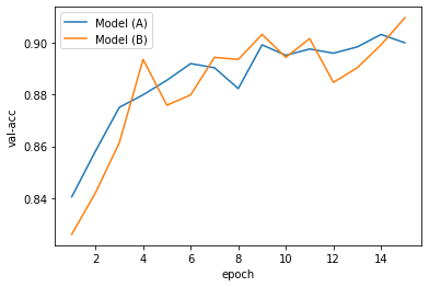
Figure 4: Chest-X-Ray Image: Validation Accuracy (median of 20 trials)

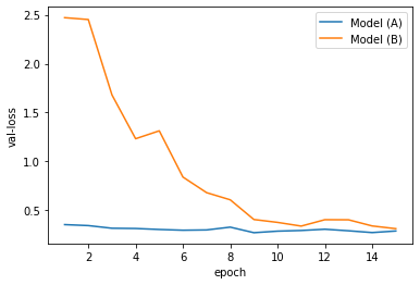
Figure 5: Chest-X-Ray Image: Validation Loss (median of 20 trials)

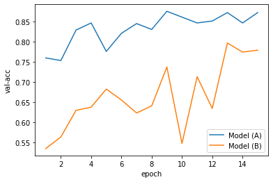
Figure 6: Chest-X-Ray Image: Validation Accuracy (worst of 20 trials)

4 Concluding Discussions

In this paper, we proposed a dimensionality reduction method applied to tensor-structured data in a convolutional neural network, and also derived the gradients of the loss function with respect to the parameters associated with the TensorProjection Layer. In addition, we implemented the TensorProjection Layer using TensorFlow, and tested it on two different data sets as a preliminary experimental study.

The first experimental result implies that the TensorProjection Layer can reduce the dimensionality of the data more efficiently than the AveragePooling Layer. The second experimental result implies that the TensorProjection Layer fits to the data faster than the fully connected layer, and the training result is also more stable. However, these results do not immediately imply that TensorProjection Layer can completely take the place of the existing methods. For example, in our preliminary experiment done before these two experiments, we found that AveragePooling Layers performed better than the TensorProjection Layer if they were embedded after the first convolutional layer. We will look into the performance of TensorProjection Layer in more details and make refinement in the future.

Appendix A Notations and Matrix Calculus

A.1 gradient

Let $x\in\mathbb{R}^{p}$ and let $L\overset{\mathrm{def}}{=}L(x):\mathbb{R}^{p}\mapsto\mathbb{R}$ be a function of $x=\left(x_{1},x_{2},\cdots,x_{p}\right)^{T}$. In this paper, we define the gradients of $L$ with respect to $x$ as below.

$$\frac{\partial L}{\partial x}\overset{\mathrm{def}}{=}\left(\frac{\partial L}{\partial x_{1}},\frac{\partial L}{\partial x_{2}},\cdots,\frac{\partial L}{\partial x_{p}}\right).$$ (66)

In this paper, the gradient of a scholar function with respect to a (column) vector becomes a row vector. Now suppose that $L(x)$ is also a multidimensional function. Let $L\overset{\mathrm{def}}{=}\left(L_{1}(x),L_{2}(x),\cdots,L_{d}(x)\right)^{T}:\mathbb{R}^{p}\mapsto\mathbb{R}^{d}$ where $x\overset{\mathrm{def}}{=}(x_{1},x_{2},\cdots,x_{p})^{T}\in\mathbb{R}^{p}$. We define the gradient of $L$ with respect to $x$ as below.

$$\frac{\partial L}{\partial x}\overset{\mathrm{def}}{=}\begin{pmatrix}\frac{\partial L_{1}(x)}{\partial x_{1}}&\frac{\partial L_{1}(x)}{\partial x_{2}}&\cdots&\frac{\partial L_{1}(x)}{\partial x_{p}}\\ \frac{\partial L_{2}(x)}{\partial x_{1}}&\frac{\partial L_{2}(x)}{\partial x_{2}}&\cdots&\frac{\partial L_{2}(x)}{\partial x_{p}}\\ \cdots&\cdots&\cdots&\cdots\\ \frac{\partial L_{d}(x)}{\partial x_{1}}&\frac{\partial L_{d}(x)}{\partial x_{2}}&\cdots&\frac{\partial L_{d}(x)}{\partial x_{p}}\end{pmatrix}$$ (67)

A.2 vectorize operation

A vectorize operator transforms a tensor (or a matrix) into a vector. For example, suppose that

$$A\overset{\mathrm{def}}{=}\begin{pmatrix}1&2&3\\ 4&5&6\end{pmatrix}.$$ (68)

Then

$$\mathrm{vec}(A) \overset{\mathrm{def}}{=} \begin{pmatrix}A_{11}&A_{21}&A_{12}&A_{22}&A_{13}&A_{23}\end{pmatrix}^{T}$$ (69)

$$= \begin{pmatrix}1&4&2&5&3&6\end{pmatrix}^{T}.$$ (70)

Similarly, if $A$ is a tensor with the size of $p\times q\times r$, then

$$A\overset{\mathrm{def}}{=}\left(A_{111},A_{211},\cdots,A_{p11},A_{121},A_{221},\cdots,A_{p21},\cdots,A_{pq1},A_{112}\cdots\right).$$ (71)

In Python (NumPy), the reshape action into $pqr\times 1$ with the option order=’F’ is the same as vectorize operation. Please refer to [4] for properties of the vec operator.

A.3 Chain Rule

Let $L\overset{\mathrm{def}}{=}L(u)$ be a scholar function with respect to a vector $u$. Suppose that $u$ is a function of another vector $x$. Then the following equation holds.

$$\frac{\partial L}{\partial x}=\frac{\partial L}{\partial u}\frac{\partial u}{\partial x}.$$ (72)

For example, let $L(u)\overset{\mathrm{def}}{=}u_{1}u_{2}$ and let $u_{1}\overset{\mathrm{def}}{=}(x_{1}+x_{2}),u_{2}\overset{\mathrm{def}}{=}(x_{2}+x_{3})$. Since $L=(x_{1}+x_{2})(x_{2}+x_{3})$, we can directly obtain

$$\frac{\partial L}{\partial x}=\left(x_{2}+x_{3},x_{1}+2x_{2}+x_{3},x_{1}+x_{2}\right).$$ (73)

We can also obtain the same result via the Chain Rule above.

$$\frac{\partial L}{\partial u}\frac{\partial u}{\partial x} = \left(u_{2},u_{1}\right)\begin{pmatrix}1&1&0\\ 0&1&1\end{pmatrix}$$ (74)

$$= (u_{2},u_{1}+u_{2},u_{1})$$ (75)

$$= (x_{2}+x_{3},x_{1}+2x_{2}+x_{3},x_{1}+x_{2}).$$ (76)

Appendix B $k$-mode product

We explain the definition of $k$-mode product between a 3-order tensor and a matrix. The following definition follows Kolda and Bader’s definition. Please refer to [5],[6]. Although, Kolda-Bader and Tensorly propose different definitions of unfolding and folding, the results of $k$-mode product are consistent.

B.1 unfolding

Let $X$ be a tensor with the size of $p_{1}\times p_{2}\times p_{3}$. Let $X_{(k)}$ be the unfolding along the $k$-th mode where $k=1,2,3$. $X_{(k)}$ is a matrix defined in the following way. In the definition below, $\mathrm{permute}(X,[\cdots])$ is an operation to swap the axes according to the order written in $[\cdots]$, and $\mathrm{reshape}$ is an operation to transform the tensor into a designated shape. In the reshape operation, we suppose that the index of the 1st mode (axis) changes faster than the 3rd (or the last) mode as well as the vectorize operation which we defined above. In NumPy’s reshape function, we need to add the option order=’F’ to follow our definition.

• $X_{(1)}\overset{\mathrm{def}}{=}\mathrm{reshape}(\mathrm{permute}(X,[1,2,3]),[p_{1},p_{2}p_{3}])$

• $X_{(2)}\overset{\mathrm{def}}{=}\mathrm{reshape}(\mathrm{permute}(X,[2,1,3]),[p_{2},p_{3}p_{1}])$

• $X_{(3)}\overset{\mathrm{def}}{=}\mathrm{reshape}(\mathrm{permute}(X,[3,1,2]),[p_{3},p_{1}p_{2}])$

We also provide a sample code in Python. Please see the Code 2. (Please import numpy as np.) In NumPy, the default reshape order option is ’C’, which is opposite from our definition. Please also refer to [13]. In [13], the reshape order is compatible with NumPy default order.

⬇

1def unfold(X, k):

2 p1 = X.shape[0];

3 p2 = X.shape[1];

4 p3 = X.shape[2];

5

6 if k == 0:

7 n_shape = np.array([p1,p2*p3]);

8 A = X.transpose(0,1,2);

9 elif k==1:

10 n_shape = np.array([p2,p3*p1]);

11 A = X.transpose(1,0,2);

12 elif k==2:

13 n_shape = np.array([p3,p1*p2]);

14 A = X.transpose(2,0,1);

15

16 X_k = np.reshape(A,n_shape,order=’F’);

17 return X_k;

Code 2: unfolding of a 3-order tensor

B.2 folding

Folding is the inverse transformation of unfolding defined above. Please see Code 3. (Please import numpy as np.)

⬇

1def fold(X_k, k, new_shape):

2 if k==0:

3 reshape_order = np.array([0,1,2]);

4 permute_order = np.array([0,1,2]);

5 elif k==1:

6 reshape_order = np.array([1,0,2]);

7 permute_order = np.array([1,0,2]);

8 elif k==2:

9 reshape_order = np.array([2,0,1]);

10 permute_order = np.array([1,2,0]);

11

12 new_shape = np.array([new_shape[reshape_order[0]],new_shape[reshape_order[1]],new_shape[reshape_order[2]]]);

13 X = np.reshape(X_k,new_shape,order=’F’);

14 X = X.transpose(permute_order);

15 return X;

Code 3: folding of a 3-order tensor

B.3 $k$-mode product

Let $X$ be a tensor with the size of $p_{1}\times p_{2}\times p_{3}$. Let $M_{k}$ be a matrix with the size of $q_{k}\times p_{k}$. Then we can define the $k$-mode product $X\times_{k}M_{k}$. $X\times_{k}M_{k}$ is a tensor with the size of $q_{1}\times p_{2}\times p_{3}$ (if $k=1$) or $p_{1}\times q_{2}\times p_{3}$ (if $k=2$) or $p_{1}\times p_{2}\times q_{3}$ (if $k=3$). The $k$-mode product is defined in the following way.

• Compute $X_{(k)}$.

• Compute $M_{k}X_{(k)}$. Note that $X_{(k)}$ is a matrix.

• Fold the matrix $M_{k}X_{(k)}$ along the $k$-th mode. (The shape is $q_{1}\times p_{2}\times p_{3}$ or $p_{1}\times q_{2}\times p_{3}$ or $p_{1}\times p_{2}\times q_{3}$.)

Please see Code 4. (Please import numpy as np.)

⬇

1def k_mode_product(X, k, M):

2 X_k = unfold(X,k);

3 qk = M.shape[0];

4 p = np.array(X.shape);

5 p[k] = qk;

6 MX_k = np.matmul(M,X_k);

7 MX_k = fold(MX_k,k,p);

8 return MX_k;

Code 4: k-mode product of a 3-order tensor

References

• [1] Haiping Lu, K. N. Plataniotis, and A. N. Venetsanopoulos. Mpca: Multilinear principal component analysis of tensor objects. Trans. Neur. Netw., 19(1):18–39, January 2008.
• [2] Shiliang Zhang and Hui Jiang. Hybrid orthogonal projection and estimation (HOPE): A new framework to probe and learn neural networks. CoRR, abs/1502.00702, 2015.
• [3] Hengyue Pan and Hui Jiang. Learning convolutional neural networks using hybrid orthogonal projection and estimation. In Min-Ling Zhang and Yung-Kyun Noh, editors, Proceedings of the Ninth Asian Conference on Machine Learning, volume 77 of Proceedings of Machine Learning Research, pages 1–16. PMLR, 15–17 Nov 2017.
• [4] K. B. Petersen and M. S. Pedersen. The matrix cookbook, nov 2012. Version 20121115.
• [5] Tensor unfolding - jean kossaifi’s home page - machine learning & computer vision. http://jeankossaifi.com/blog/unfolding.html. (Accessed on 03/16/2020).
• [6] Tamara G. Kolda and Brett W. Bader. Tensor decompositions and applications. SIAM Rev., 51(3):455–500, August 2009.
• [7] Changqing Xu, Lingling He, and Zerong Lin. Commutation matrices and commutation tensors. Linear and Multilinear Algebra, page 1–22, Dec 2018.
• [8] Martín Abadi, Ashish Agarwal, Paul Barham, Eugene Brevdo, Zhifeng Chen, Craig Citro, Greg S. Corrado, Andy Davis, Jeffrey Dean, Matthieu Devin, Sanjay Ghemawat, Ian Goodfellow, Andrew Harp, Geoffrey Irving, Michael Isard, Yangqing Jia, Rafal Jozefowicz, Lukasz Kaiser, Manjunath Kudlur, Josh Levenberg, Dandelion Mané, Rajat Monga, Sherry Moore, Derek Murray, Chris Olah, Mike Schuster, Jonathon Shlens, Benoit Steiner, Ilya Sutskever, Kunal Talwar, Paul Tucker, Vincent Vanhoucke, Vijay Vasudevan, Fernanda Viégas, Oriol Vinyals, Pete Warden, Martin Wattenberg, Martin Wicke, Yuan Yu, and Xiaoqiang Zheng. TensorFlow: Large-scale machine learning on heterogeneous systems, 2015. Software available from tensorflow.org.
• [9] Han Xiao, Kashif Rasul, and Roland Vollgraf. Fashion-mnist: a novel image dataset for benchmarking machine learning algorithms. CoRR, abs/1708.07747, 2017.
• [10] Chest x-ray images (pneumonia) | kaggle. https://www.kaggle.com/paultimothymooney/chest-xray-pneumonia. (Accessed on 03/23/2020).
• [11] Karen Simonyan and Andrew Zisserman. Very deep convolutional networks for large-scale image recognition. CoRR, abs/1409.1556, 2014.
• [12] J. Deng, W. Dong, R. Socher, L.-J. Li, K. Li, and L. Fei-Fei. ImageNet: A Large-Scale Hierarchical Image Database. In CVPR09, 2009.
• [13] Jeremy E. Cohen. About notations in multiway array processing, 2015.