The Raman signal from a hindered hydrogen rotor

Abstract

We present a method for calculation of Raman modes of the quantum solid phase I solid hydrogen and deuterium. We use the mean-field assumption that the quantised excitations are localized on one molecule. This is done by explicit solution of the time-dependent Schroedinger equation in an angle-dependent potential, and direct calculation of the polarisation. We show that in the free-rotor limit, the H₂ and D₂ frequencies differ by a factor of 2, which evolves toward $\sqrt{2}$ as the modes acquire librational character due to stronger interactions. The ratio overshoots $\sqrt{2}$ if anharmonic terms weaken the harmonic potential. We also use density functional theory and molecular dynamics to calculate the E${}_{2_{g}}$ optical phonon frequency and the Raman linewidths. The molecular dynamics shows that the molecules are not free rotors except at very low pressure and high temperature, and become like oscillators as phase II is approached. We fit the interaction strengths to experimental frequencies, but good agreement for intensities requires us to also include strong preferred-orientation and stimulated Raman effects between S₀(1) and S₀(0) contributions. The experimental Raman spectrum for phase II cannot be reproduced, showing that the mean-field assumption is invalid in that case.

I Introduction

The lowest pressure phase of solid hydrogen comprises a hexagonal close packed (hcp) structure of molecules Hazen et al. (1987); Loubeyre et al. (1996); Mao and Hemley (1994); Sharma et al. (1980); Hemley et al. (1990a, 1993); W. N. Hardy, I. F. Sivlera, K. N. Klump (1968). X-ray and neutron studies can detect the mean nuclear position, but the orientational behavior is more complicated. Raman spectroscopy at the lowest pressures, shows that the molecules adopt free rotor behavior, characterized by a series of contributions corresponding to energy levels $J(J+1)$ and selection rule $\Delta J=2$. As pressure increases the identification of the single rotational levels become more complicated, as these low frequency bands significantly broadenGoncharov et al. (1996); Mazin et al. (1997); Goncharov et al. (1998); Pena-Alvarez et al. (2019).

The free rotor and the simple harmonic oscillator are the two canonical systems considered in Raman Spectroscopy, but it is impossible to determine the character of the mode directly from an experimental peak. For the diatomic rotor the roton energy levels are given by:

$$E(J)=\frac{\hbar^{2}}{mr^{2}}J^{2}$$ (1)

in 2D and in 3D by:

$$E(J)=\frac{\hbar^{2}}{mr^{2}}J\left(J+1\right)$$ (2)

where $r$ is the bond length, m is the atomic mass and $J$ is an integer quantum number. The Raman selection rule is $\Delta J=0,\pm 2$, where zero corresponds to Rayleigh scattering, $+2$ to Stokes, and -2 to Anti-Stokes processes. This expression holds for both two dimensions (2D) and three dimensions (3D) rotors, and the energies are fully determined by the bondlength $r$.

For the harmonic oscillator the phonon levels are:

$$E(n)=\hbar\omega\left(n+\frac{1}{2}\right)=\sqrt{\frac{\hbar^{2}k}{m}}\left(n+\frac{1}{2}\right)$$ (3)

with $\omega$ the frequency and $k$ the effective spring constant, selection rules being $\Delta n=0,\pm 1$.

A peculiarity of these expressions is the different dependence of energy on mass. This becomes particularly relevant when considering the isotopes of hydrogen, H₂ and D₂. If one assumes that their electronic structures are the same, and the Born-Oppenheimer approximation holds, then at the same density the roton frequencies differ by a factor of 2, while phonon/libron frequencies differ only by $\sqrt{2}$. Thus the character of a mode can be determined by comparing the Raman spectrum of the isotopes. Experimental studies of this ratio are presented in the accompanying paperPena-Alvarez et al. (2019).

In this paper, we develop the theory for the Raman signal from an inhibited quantum rotor, assuming that the interactions can be represented by an external potential. We illustrate the principles with a 2D example, then apply it to a 3D case where the potential will be taken to have the form of interacting quadrupoles and a crystal field on an hcp lattice. To calculate Raman phonon frequencies and to estimate natural linewidths we use ab initio molecular dynamics simulations.

II Theory and Methods

II.1 Crossover from roton to libron

To illustrate the principles, we consider a single mode described by the Hamiltonian for a 2D hindered rotor in an external potential $\hat{V}=V_{0}\cos\theta$:

$$\frac{\hbar^{2}}{mr^{2}}\frac{\partial^{2}\Psi(\theta)}{\partial\theta^{2}}-V_{0}\cos\theta\Psi(\theta)=E\Psi(\theta)$$ (4)

The solutions for $E_{k}(V_{0})$ are shown in Figure 1. The frequency ratio for the excitation between rotors with mass 1 (“hydrogen”) and 2 (“deuterium”) is then defined by:

$$R=\frac{E_{k}(H)-E_{i}(H)}{E_{k}(D)-E_{i}(D)}=\upsilon_{H_{2}}/\upsilon_{D_{2}}$$ (5)

where $E_{i}$ are the calculated energy levels and $\upsilon$ represents the experimentally-measurable Raman shift.

The limiting cases have $R=2$ for the rotor ($V_{0}=0$) and $R=\sqrt{2}$ ($V_{0}\rightarrow\infty$), and a surprising result is that $R$ overshoots and becomes less than its asymptotic value of $\sqrt{2}$: this happens whenever anharmonic terms make the potential weaker than harmonic at large distances. Extreme cases for this are the $1/r$ potential where the asymptotic value is $R=\frac{1}{2}$ and the purely quartic potential where this ratio becomes $R=2^{2/3}$.

Fig.1 also shows that the high $J$ states remain as free rotors long after the first excited state passes through the “oscillator” value $R=\sqrt{2}$.

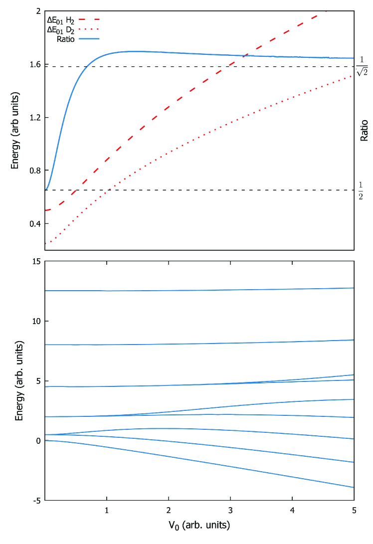
Figure 1: 2D rotor in a potential of the form $V=V_{0}cos(\theta)$. Top: left axis shows energy of first excitation, compared between $m=1,2$, right axis shows ratio of first excitations. Bottom: Energy levels as a function of $V_{0}$; energy units are defined by $\frac{\hbar^{2}}{2m_{H}r^{2}}=1$

II.2 Spin isomers in solid hydrogen and deuterium

In solid state hydrogen, the situation becomes more complex. Below 2 GPa the Raman spectrum can be characterized by a molecular roton spectrum, a lattice phonon mode, and molecular vibrons at high frequencyVan Kranendonk and Karl (1968). At low pressure and temperature the peaks are very sharp, so mode-coupling and perturbative crystal field splitting is also observable. Van Kranendonk (1983); Pena-Alvarez et al. (2019) Comparing hydrogen and deuterium, the factor $R=2$ is observed, demonstrating that the excitations are rotons.

For a free hydrogen molecule the overall wavefunction involves both nuclear spin and rotational state degrees of freedom. The nuclear spin wavefunction can be either a spin-1 symmetric triplet ($ortho$-H) or spin-0 antisymmetric singlet ($para$-H). There is no significant energy associated with nuclear spins, but since protons are fermions with spin $\frac{1}{2}$, the overall wavefunction must be antisymmetric, so only $para$-H can combine with the symmetric $J=0$ rotor ground state. Consequently, in phase I where intermolecular coupling is weak enough that rotor energy states are localised on a single molecule, then $para$-H has lower energy than $ortho$-H. At the phase II boundary, R=$\sqrt{2}$, so the observed excitations are oscillators, not rotors. $J$ is not a good quantum number, and delocalization of oscillations means that exchange symmetry does not introduce an independent constraint on each molecule . Consequently, $ortho$-H has a higher I-II transition temperature than $para$-HLorenzana et al. (1989, 1990). A broadly similar situation exists in deuteriumSilvera and Wijngaarden (1981), except that the deuteron is a spin-1 boson, so $ortho$-D couples to the ground state $J=0$, and comprises singlet and quintuplet antisymmetric states as shown in table 1.

These nuclear spin degeneracies result in $ortho-para$ ratios of 3:1 in H₂ and 1:2 in $D_{2}$ at room temperature, which persist metastably on coolingStrzhemechny et al. (2002).

	H2-$ortho$	H2-$para$	D2-$ortho$	D2-$para$	HD
spin symm.	even	odd	even	odd	none
spin degen.	3	1	6	3	6
rotor symm.	odd	even	even	odd	any
rotor state	J=1	J=0	J=0	J=1	J=0
rotor degen.	3	1	1	3	1

Table 1: Exchange symmetries of wavefunctions showing which nuclear spin states can trap the quantum rotor in high energy $J=1$ state, assuming sufficiently weak interactions that $J$ is a good quantum number.

II.3 The hindered-rotor Hamiltonian and wavefunction

Under pressure, intermolecular interactions inhibit the rotors. In classical molecular dynamics, this manifests as increasingly chaotic angular motion of the molecules, while the molecular centre and bondlengths behave like harmonic oscillators.

To understand the hindered rotor, we model the system by describing the rotational motion of a molecule in the potential of its neighbours on an hcp lattice. Specifically, we solve the angular Schroedinger equation:

$$H(\theta,\phi)= -\frac{\hbar^{2}}{mr^{2}}\left[\frac{1}{\sin\theta}\frac{\partial}{\partial\theta}\left(\sin\theta\frac{\partial}{\partial\theta}\right)+\frac{1}{{\sin^{2}\theta}}\frac{\partial^{2}}{\partial\phi^{2}}\right]$$ (6)

$$+V(\theta,\phi)$$

where $r=\mathbf{|r|}$ is the molecular bond length and $m$ is the mass of the nucleus.

The potential should have the $P63/mmm$ symmetry of the hcp lattice, and its strength will increase with density. We model it as two distinct contributions, describing the electrostatic and steric interactions. Long ranged electrostatic interactions, of which quadrupole-quadrupole interactions are dominant, are accounted for by a term with a single parameter, $\lambda$,

$$V_{e}(\theta,\phi)=\lambda\sum_{i}\left[\frac{1}{({\bf R}_{i}-\frac{\bf r}{2})^{5}}+\frac{1}{({\bf R}_{i}+\frac{\bf r}{2})^{5}}\right]$$ (7)

Where ${\bf R}_{i}$ is the vector from the central molecule and the $i^{th}$ molecule in the unit cell. The values of $R_{i}$ are taken from the experimental equation of state Loubeyre et al. (2013) and bondlength $\mathbf{|r|}$ was fitted to the experimental spectra at each pressure and temperature, to within $5\%$ of the gas phase value of $0.74$ Å. This also affects the moment of inertia, $I=mr^{2}$, in the kinetic energy term in equation 6.

At short range, steric interactions due to Pauli repulsion become important, and quadrupole interactions are enhanced by orientational correlations. We include this by fitting $c_{20}(P)$ and $c_{40}(P)$ directly:

$$V_{s}(\theta,\phi)=c_{20}Y_{20}+c_{40}Y_{40}$$ (8)

This approach allows the entire potential $V=V_{e}+V_{s}$ to be described with three parameters: $\lambda,c_{20},c_{40}$. Interestingly, although $c_{20}$ is allowed in P6₃/mmm symmetry, it is zero for central interactions on an hcp lattice with ideal $c/a$ ratio.

We attempted to include quadrupole correlations at a pairwise level, which gives a parameter-free model. By neglecting frustration, this strongly overestimates the total quadrupole-quadrupole energy but, surprisingly the angular dependence is too weak to explain the experimental splittings (see Fig. S1).

We expand the potential energy surface $V(\theta,\phi)$ in the basis of spherical harmonics $Y_{kq}(\theta,\phi)$ since these are the solutions to the free rotor problem Rouvelas (2013),

$$V(\theta,\phi)=\sum_{kq}v_{kq}Y_{kq}(\theta,\phi)$$ (9)

by performing the surface integrals:

$${}v_{kq}=\int Y^{*}_{kq}(\theta^{\prime},\phi^{\prime})V(\theta^{\prime},\phi^{\prime})\sin(\theta^{\prime})d\theta^{\prime}d\phi^{\prime}$$ (10)

We can now express the full Hamiltonian in the basis of the free rotor:

$$H_{lml^{\prime}m^{\prime}}^{(0)}=\frac{\hbar^{2}}{2{\mu}r^{2}}l(l+1)\delta_{ll^{\prime}}\delta_{mm^{\prime}}+V_{lml^{\prime}m^{\prime}}$$ (11)

where the first term is the free rotor kinetic energy and the second is the potential energy operator, expressed as:

$$V_{lml^{\prime}m^{\prime}} =\langle lm|V(\theta,\phi)|l^{\prime}m^{\prime}\rangle$$ (12)

$$=\sum_{kq}v_{kq}\langle lm|kq\rangle|l^{\prime}m^{\prime}\rangle$$

where we employed equation 9 to expand the potential energy surface. The $\langle lm|kq\rangle|l^{\prime}m^{\prime}\rangle$ are Clebsch-Gordan coefficients. The energy levels are found by diagonalizing the Hamiltonian:

$$H_{nn^{\prime}}^{(0)}=D^{*}_{n,lm}H_{lml^{\prime}m^{\prime}}^{(0)}D_{l^{\prime}m^{\prime},n^{\prime}}$$ (13)

Note that $l$ and $m$ are no longer good quantum numbers and so we introduce a new quantum number $n$. The new energy levels are $\omega_{n}=H^{0}_{nn}$, and $D_{l^{\prime}m^{\prime},n^{\prime}}$ is the transformation from the free rotor basis $\lvert lm\rangle$ to the hindered rotor basis $\lvert n\rangle$. The rotational eigenfunctions of the hindered rotor can be evaluated as:

$$\psi_{n}=D^{*}_{n,lm}Y_{lm}$$ (14)

and their parity (i.e. rotor symmetry) from:

$$\psi_{n}(\theta,\phi)=(-1)^{par}\psi_{n}(\pi-\theta,\phi+\pi)$$ (15)

Based on the parity we can split the diagonal Hamiltonian into $ortho$ and $para$ contributions:

$$\widehat{H}^{(0)}=\widehat{H}^{(0)}_{o}+\widehat{H}^{(0)}_{p}$$ (16)

and write the total equilibrium density matrix as:

$$\hat{\rho}^{(0)}=\frac{g_{o}e^{-\widehat{H}^{(0)}_{o}/kT}+g_{p}e^{-\widehat{H}^{(0)}_{p}/kT}}{Z(T)}$$ (17)

where $g_{0}$ and $g_{p}$ are the nuclear spin degeneracies as laid out in table 3 and $Z(T)=Z_{o}(T)+Z_{p}(T)$ is the total partition function with the components:

$$Z_{o}(T)=g_{o}\operatorname{Tr}\left(e^{-\widehat{H}^{(0)}_{o}/kT}\right)$$ (18)

$$Z_{p}(T)=g_{p}\operatorname{Tr}\left(e^{-\widehat{H}^{(0)}_{p}/kT}\right)$$

This assumes equilibration of the $ortho$/$para$ concentrations, however, the nuclear spins equilibrate of the timescale of a typical experimentEggert et al. (1999), and so $ortho$-peaks are initially visible even at 10 K. We account for this by redefining the density matrix as:

$$\hat{\rho}^{(0)}=\frac{Z_{o}(T^{\prime})}{Z(T^{\prime})}\frac{g_{o}e^{-\widehat{H}^{(0)}_{o}/kT}}{Z_{o}(T)}+\frac{Z_{p}(T^{\prime})}{Z(T^{\prime})}\frac{g_{p}e^{-\widehat{H}^{(0)}_{p}/kT}}{Z_{p}(T)}$$ (19)

where we introduced a separate parameter $T^{\prime}$ that describes the $ortho$-$para$ ratio observed in the experiment as the thermodynamic temperature of the spins; $T^{\prime}$ eventually equilibrates to $T$ at a rate which depends on experimental details.

Now we turn our attention to the polarizability tensor $\widehat{\Pi}_{ij}$. The laser interacts with the system Hamiltonian via a second order field perturbation:

$$\widehat{H}(t)=\widehat{H}^{(0)}-E_{i}(t)\widehat{\Pi}_{ij}E_{j}(t)$$ (20)

In the free rotor basis of spherical harmonics, the polarizability tensor can be expressed as:

$$\Pi_{ij,lml^{\prime}m^{\prime}}=\langle lm\rvert\mathbf{R}^{T}(\theta,\phi)\cdot\boldsymbol{\alpha}\cdot\mathbf{R}(\theta,\phi)\lvert l^{\prime}m^{\prime}\rangle$$ (21)

The polarizability tensor depends on the nature of the molecules in the sample. Specifically, for a linear molecule

$$\boldsymbol{\alpha}=\left(\begin{matrix}1&0&0\\ 0&1&0\\ 0&0&\alpha\\ \end{matrix}\right)$$ (22)

is the polarizability in the reference frame of the hydrogen molecule. $\alpha$ is a known parameter, taken to have a value of 1.43 from previous experimental work Bridge and Buckingham (1966); Miliordos and Hunt (2018) and considered to be pressure and temperature independent here. The rotation matrix $\mathbf{R}$ transforms the $E$-fields into the frame of the molecule, before they interact with the polarizability ellipsoid. These rotations are effectively averaged in the frame of the single rotor by the orientation probabilities dictated by the wavefunctions.

Alternatively, we can express the polarizability tensor in the hindered rotor basis $\lvert n\rangle$:

$$\Pi_{ij,nn^{\prime}}=D^{*}_{n,lm}\Pi_{ij,lml^{\prime}m^{\prime}}D_{l^{\prime}m^{\prime},n^{\prime}}$$ (23)

by applying the same transformation that diagonalizes the Hamiltonian.

Depending on the orientations of the fields $E_{i}$ and $E_{j}$ and the geometry of the experiment, different elements of the tensor will contribute. Raman spectra from diamond anvil cell experiments are obtained in back-scatter geometry, while the sample normally has preferred orientation along the beam direction. These conditions impose restrictions over which of the $i$ and $j$ components of the polarizability tensor, contribute to the response. The cases we considered are summarized in table 2.

crystal orientation	total response
$c||Z$	$\sum_{J=X,Y}R\left(\widehat{\Pi}_{XJ}\right)$
isotropic	$\sum_{I,J=X,Y,Z}R\left(\widehat{\Pi}_{IJ}\right)$

Table 2: Components of the polarizability that contribute to the total response for each of the crystal orientation.

Additionally we suppress all $ortho$ to $para$ transitions by setting the corresponding elements in the transition matrix to zero. We only allow transitions that leave the symmetry of the nuclear spin wave-function unchanged.

So far we derived the system Hamiltonian $H^{(0)}_{nn^{\prime}}$ and the effective polarisability tensor ${\Pi}_{ij,nn^{\prime}}$ based on the $v_{kq}$ coefficients. We have, thus, obtained the energy levels of the hindered rotor, and the transition probabilities between them.

II.4 Calculation of Raman signal

We proceed to calculating the actual Raman signal from the response of the quantum system to a sudden excitation. We rely on the time-frequency duality to compute the Raman response in the time domain and then obtain the Raman spectrum by Fourier transform (FT) of the time response. We achieve this by first propagating the density matrix of the system under the influence of the field and then computing the expectation value of the resulting polarization Mukamel (1995); Hamm and Zanni (2011); Finneran et al. (2016, 2017). The dynamics is given by the Liouville-von Neumann (LvN) equation:

$$\frac{d\hat{\rho}}{dt}=-\frac{i}{\hbar}\left[\widehat{H},\hat{\rho}\right]$$ (24)

The advantage of using LvN over the time-dependent Schrodinger equation is that the density matrix can also describe a statistical ensemble of rotors given by:

$$\rho_{nn^{\prime}}=\sum_{s}p_{s}\rho^{s}_{nn^{\prime}}$$ (25)

where $\rho^{s}_{nn^{\prime}}$ is the density matrix of the system $s$ and $p_{s}$ is the probability of finding system $s$. Using the Chain Rule and substituting equation 24, we can express the dynamics of the mixed density matrix $\rho_{nn^{\prime}}$ as Hamm and Zanni (2011); Mukamel (1995):

$$\frac{d\rho_{nn^{\prime}}}{dt}=\sum_{s}p_{s}\frac{d\rho^{s}_{nn^{\prime}}}{dt}+\sum_{s}\frac{dp_{s}}{dt}\rho^{s}_{nn^{\prime}}$$

$$=-\frac{i}{\hbar}\left[H,\rho\right]_{nn^{\prime}}+\sum_{s}\frac{dp_{s}}{dt}\rho^{s}_{nn^{\prime}}$$ (26)

The first term describes the quantum mechanical evolution of the system, while the second term describes the classical statistics and relates to coherence dephasing and energy dissipation. In Redfield formalism, this term can be approximated as:

$$\sum_{s}\frac{dp_{s}}{dt}\rho^{s}_{nn^{\prime}}=-\frac{\rho_{nn^{\prime}}}{\tau}=-\rho_{nn^{\prime}}\Gamma$$ (27)

where $\Gamma$ represents the natural line width broadening. Now we include the total Hamiltonian which contains the external field perturbation, in equation II.4, and obtain:

$$\frac{d\rho_{nn^{\prime}}}{dt}=-\frac{i}{\hbar}\left[H^{(0)},\rho\right]_{nn^{\prime}}+\frac{i}{\hbar}\left[\Pi\delta(t),\rho\right]_{nn^{\prime}}-\rho_{nn^{\prime}}\Gamma$$ (28)

Where we assumed the laser field is impulsive and can be treated as a delta function $\delta(t)$. When the field strength is weak and it does not change the original eigenvalues, we can use perturbation theory to describe the evolution of the density matrix Mukamel (1995); Hamm and Zanni (2011). We write:

$$\rho_{nn^{\prime}}(t)=\rho^{(0)}_{nn^{\prime}}+\rho^{(1)}_{nn^{\prime}}(t)$$ (29)

where $\hat{\rho}^{(0)}$ is the equilibrium density and $\rho^{(1)}(t)$ describes the response of the system to the external perturbation. Additionally, the equilibrium Hamiltonian is diagonal in the $\lvert n\rangle$ basis, so the first commutator can be easily solved and equation 28 becomes:

$$\frac{d\rho^{(1)}_{nn^{\prime}}}{dt}= -\left(i(\omega_{n}-\omega_{n^{\prime}})+\Gamma\right)\rho^{(1)}_{nn^{\prime}}$$ (30)

$$+\frac{i}{\hbar}\left[\Pi\delta(t),\rho^{(0)}\right]_{nn^{\prime}}$$

We understand this equation intuitively as follows. The equilibrium density matrix $\rho_{0}$ is diagonal and commutes with the system Hamiltonian and therefore does not contribute to the dynamics. As a result, in the absence of the external perturbation the system is in equilibrium and does not change. The effective polarizability operator acts upon the equilibrium density matrix at $t=0$ and creates off diagonal terms (coherent superpositions of states) $\rho^{(1)}_{nn^{\prime}}(t=0)$ which then evolve under the system Hamiltonian with oscillating phases $-i(\omega_{n}-\omega_{n^{\prime}})$ which decay at a rate $\Gamma$. We integrate equation 30 via a change of variables and obtain:

$$\rho^{(1)}_{nn^{\prime}}(t)=\frac{i}{\hbar}\int_{-\infty}^{t}\left[\delta(\tau)\Pi,\rho^{(0)}\right]_{nn^{\prime}}e^{-[i(\omega_{n}-\omega_{n^{\prime}})+\Gamma](t-\tau)}d\tau$$ (31)

and since we assume the perturbation is instantaneous in time, this simplifies to:

$$\rho^{(1)}_{nn^{\prime}}(t)=\frac{i}{\hbar}\left[\Pi,\rho^{(0)}\right]_{nn^{\prime}}e^{-[i(\omega_{n}-\omega_{n^{\prime}})+\Gamma]t}$$ (32)

We discard the second part of the commutator since it is just the complex conjugate of the first part and it carries the same information. The remaining part contains both the Stokes and anti-Stokes Raman contributions. In our energy-sorted basis $\lvert n\rangle$ all Stokes contributions are in the lower triangular matrix and the anti-Stokes are in the upper triangular matrix, so we discard the upper half to keep the pure Stokes signal:

$$\rho^{(1)}_{n,n^{\prime}<n}(t)=\frac{i}{\hbar}\Pi_{nm}\rho^{(0)}_{mn^{\prime}}e^{-[i(\omega_{n}-\omega_{n^{\prime}})+\Gamma]t}$$ (33)

Finally, the expectation value of the system polarization expressed in time domain, is:

$$S(t)={\rm Tr}\left(\Pi_{nm}\rho^{(1)}_{m,n^{\prime}<m}(t)\right)$$ (34)

while in frequency domain the observed spectrum is given by:

$$R(f)=\Re{\left(\int_{-\infty}^{\infty}S(t)e^{-ift}dt\right)}$$ (35)

This gives the entire Raman spectrum with Lorentzian line shapes arising from the broadening $\Gamma$. Pressure broadening gives a similar line shape, so we include this into our simulations by adding a pressure dependent contribution to $\Gamma$:

$$\Gamma=\Gamma^{0}+\Gamma^{P}$$ (36)

This broadening parameter corresponds to the width of peaks and we calculated it with two approaches. On one hand, the simplest approach is simply to regard this as a fitting parameter, choosing peak widths that match the experimental data. On the other hand, trends in lifetime broadening can be calculated from the decay of the angular momentum autocorrelation function extracted from ab initio molecular dynamics (AIMD) simulations as described in section IV. There are many approximations in this latter approach, but one robust feature from AIMD is that all timescales are $\sqrt{2}$ longer for deuterium than for hydrogen, so other things being equal the deuterium peaks will be sharper than the hydrogen ones.

III Results

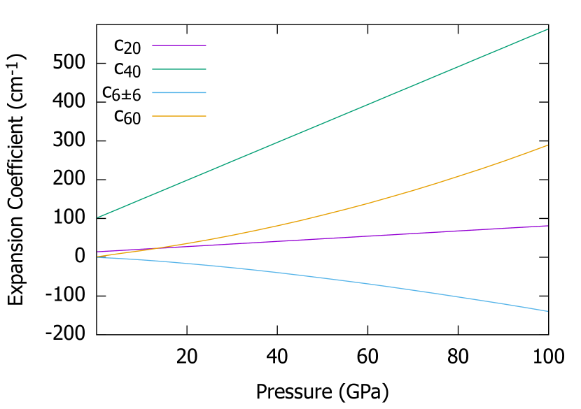
Figure 2: Expansion coefficients $v_{lm}$ (Eq. 10) of spherical harmonics for the potential $V(\theta,\phi)$ (largest 5 are shown with the exception of Y₀₀).

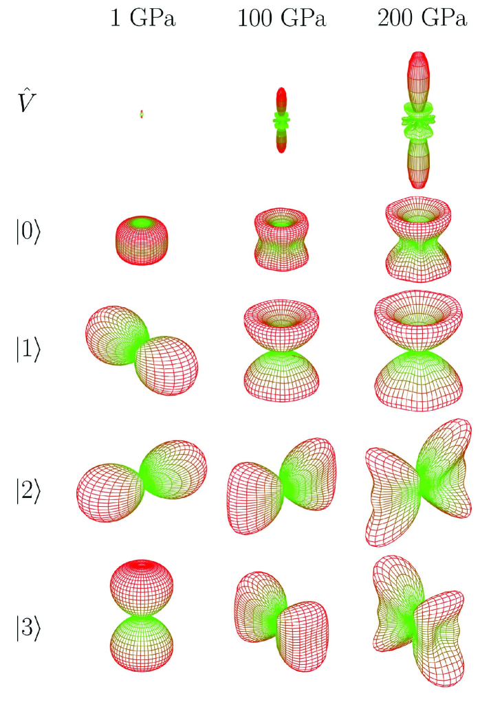
Figure 3: 3D representation of the potential $V_{P}(\theta,\phi)$ (top) and four lowest energy wavefunctions $|\Phi(\theta,\phi)|^{2}$ (below) with increasing potential/pressure (left to right) (note the large isotropic $Y_{00}$ component of the potential is not shown here to emphasise the angular dependence).The second excited state is doubly degenerate and thus the resulting eigenfunctions from the numerical diagonaliser represent one of many possible combinations of basis functions. The bond length was assumed to remain constant at $0.74$ Å  over all pressures as in Fig. 4.

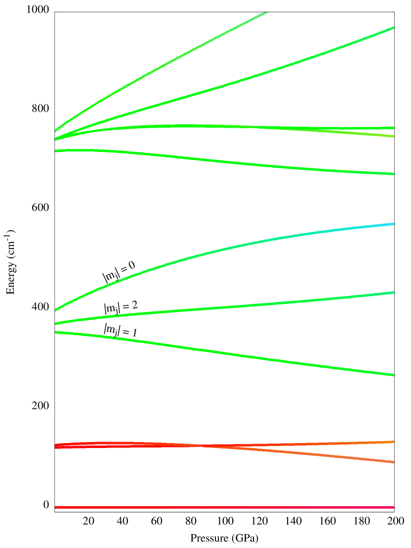
Figure 4: Energy levels for a hydrogen rotor in a hexagonal potential: different colors indicate the mixing of the spherical harmonics in the eigenstate on an RGB scale where red, green and blue pixel values represent contributions from $Y_{00}$ and $Y_{1m}$, $Y_{2m}$ and $Y_{3m}$, $Y_{4m}$ up to $Y_{6m}$ respectively (note: the RGB values have also been rescaled to show $0-10\%$ mixing). For this figure the bond length was assumed to remain constant at $0.74$ Å  as experimental data is not available for the pressures considered here.

At low pressure, we obtain ideal rotor behavior, followed by a perturbative region where, e.g. the $J=0\rightarrow 2$ $S_{0}(0)$ level splits into a triplet. The pattern becomes increasingly complicated as pressure increases: not only are the levels split by the field, but the pure Y_lm wavefunctions are mixed, which gives Raman activity to previously forbidden transitions. Also, the splitting means a group of low energy transitions corresponding to $\Delta J=0$ appear with non-zero shiftSilvera and Wijngaarden (1981).

For the electrostatic contribution to the potential ($V_{e}$) a single value of $\lambda=1.98\times 10^{5}\hskip 2.0pt$cm^-1Å^-5 was used for all pressures and temperatures. Expansion coefficients for the total resultant potential surface $V(\theta,\phi)$ over a range of pressures are shown in Fig. 2. The same parameters describe both hydrogen and deuterium and are independent of temperature. Obviously, much better fits can be obtained using more or unphysical parameters, but doing so could conceal where our single-rotor approximation breaks down. This failure is particularly evident in deuterium above $\sim 30$ GPa as phase II emerges (see accompanying paper for details and section V where we show the comparison between our calculated spectra and the experimental ones.).

Fig. 3 shows the potential surface corresponding to the parameters listed above along with the resulting wavefunctions with increasing pressure. At low pressure there is close to zero angular dependence from the potential and the wavefunctions broadly resemble the spherical harmonics. As the pressure is increased up to 100 GPa, minima in the potential surface (shown in green) are seen pointing out of the a-b plane at an angle of $\sim 55^{\circ}$ and at six distinct orientations within the a-b plane. A large maximum in the potential energy surface occurs when the molecule is parallel to the c axis. The emergence of these minima with increasing pressure gives rise to corresponding distortions of the wavefunctions with an increased probability density at $\sim 55^{\circ}$ to the a-b plane seen in the ground and first excited states. This tendency of the wavefunction to flatten is consistent with AIMDMagdău and Ackland (2013); Ackland and Loveday (2019), Monte Carlovan de Bund and Ackland (2020) and experimentJi et al. (2019) in phase I, and opposite to theories which predict the molecule pointing preferentially out of planeFreiman et al. (1998).

Fig. 4 shows the variation of the energy levels with applied potential, with coloring indicating the mixing of spherical harmonics. Relatively little mixing ($5-10\%$) still results in a significant change in the angular dependence of the probability density.

III.1 Raman mode between split rotational levels

Raman modes associated with molecular rotations are typically characterized as librons and rotons. Our calculations show a type of mode which fits neither of these - a reorientational mode. In the free rotor case, this would be an elastic scattering transition with $\Delta J=0$. As the potential increases, the Raman shift becomes non-zero: with increasing pressure the low frequency mode between levels of different $M_{J}$ emerges from the Rayleigh line (Fig. 5). The selection rule means it can only occur from an initial excited state with $J>0$. The equivalent mode at zero pressure has been measured using microwave resonance experimentsHardy and Berlinsky (1975); Hardy et al. (1977). At higher pressures the mode may be thought of as the molecule reorienting between inequivalent minima in the potential surface. We note that in the backscattering geometry, with a sample with c axes parallel to the beam, this mode will not be observed.

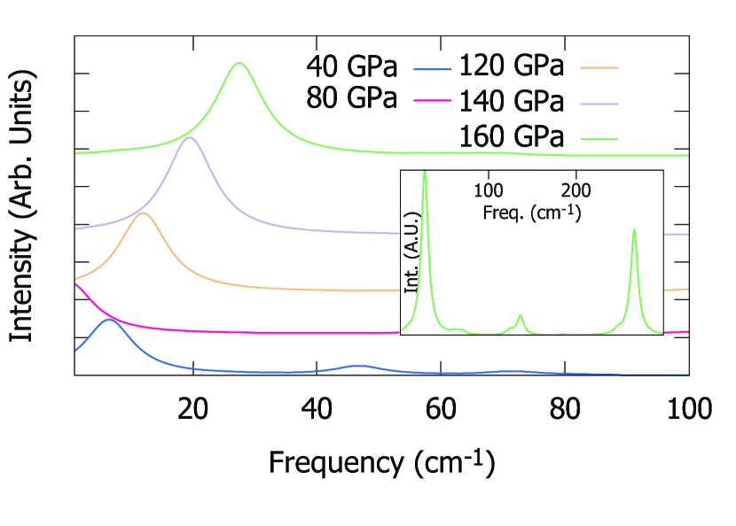
Figure 5: Predicted rotational/librational Raman spectrum at frequencies close to the Rayleigh line for hydrogen at 300 K over a range of pressures (broadening parameter is set to $\Gamma=30$ cm^-1 for all pressures to allow transitions to be easily identified). Inset shows the $S_{0}(0)$ triplet and new mode at 160 GPa to demonstrate relative intensities. The bond length was assumed to remain constant at $0.74$ Å  over all pressures. All spectra shown assume a perfect powder measured in backscatter as the reorientational mode is not visible for a sample with c-axis parallel to the incident beam measured in backscatter. At pressures greater than 80 GPa the reorientational mode appears at increasingly larger frequency shifts. At 80 GPa a crossing in the $J=1$ energy levels (seen in Fig. 4) produces a frequency shift much closer to the Rayleigh line.

IV Molecular dynamics simulations

We have carried out further analysis using a series of ab initio molecular dynamics (AIMD) simulations in phase I of hydrogen, using methods presented previouslyClark et al. (2005); Magdău and Ackland (2013); Ackland and Magdău (2015); Magdău and Ackland (2014); Magdău et al. (2017).

Molecular dynamics of the quantum rotor phase used classical nuclei, which have long been known to give good results for properties such as the melting pointBonev et al. (2004); Liu et al. (2012, 2013) and to form a basis for a fully quantum theory. Zero point energy favours phase I, but is omitted in AIMD. Thus the symmetry-breaking phase II of hydrogen is observed even at zero pressure in classical AIMD. Here we use AIMD to calculate the phonon frequency and to estimate the coherence dephasing parameter which controls our linewidth calculation.

IV.1 Calculation of Linewidths

In previous work on vibrational modes, we have shown that the observed broadening is primarily due to the lifetime of the modeMagdău and Ackland (2013). So the parameter $\Gamma$ can be calculated using ab initio molecular dynamics. For vibrational modes, the Raman shift can be extracted directly from the vibrational frequency. This can be found by Fourier Transform of the velocity autocorrelation function, which conveniently also extracts the lifetime broadening from the anharmonicity.

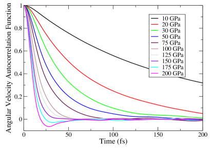
Figure 6: Angular momentum autocorrelation functions for diatomic rotors at 300 K and a range of pressures. An ideal rotor has an unchanging correlation function at 1, a harmonic oscillator would have a sinusoidal function between 1 and -1. Clearly neither is the case here.

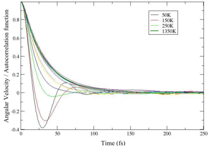
Figure 7: Angular momentum correlation functions vs time (fs) at 100 GPa and a range of temperatures, selected ones labelled, showing convergence on extension into the liquid phase. The fastest decay is at 250 K, where all correlation is lost long before a single rotation is complete. In phase II (below 150 K, red and black lines), the autocorrelation becomes negative, indicating that the molecules are librating and not rotating.

The simple harmonic oscillator is a special case in that its quantum energy is directly related to vibrational frequencies (in Molecular Dynamics) or derivative of the potential energy (in Lattice Dynamics). However, the quantised energy levels of a free rotor (Eq.2) are unrelated to any classical frequency. For this reason, the hindered rotor Raman shift cannot be evaluated from AIMD. However, it is possible to calculate the roton/libron lifetime, and hence the pressure broadening of the Raman linewidth, from the autocorrelation function in molecular dynamics (Figs.6 and 7).

From each MD run we identified molecules, and calculated the autocorrelation function of the angular momentum.

$$\ell(t)=\int\frac{\langle\sum_{i}{\bf L}_{i}(t-t^{\prime}){\bf L}_{i}(t^{\prime})\rangle}{\langle\sum_{i}L^{2}(t^{\prime})\rangle}dt^{\prime}$$ (37)

where L is the angular momentum, the sum runs over all molecules and the integral is over the simulation after an equilibriation period.

For a rotor, the autocorrelation function decays to zero, while for a libron there is an anticorrelation period. In either case, the classical correlation time is a good proxy for the quantum lifetime, and the lifetime broadening can be found by Fourier transform of $\ell(t)$. Here the peaks become infinitely sharp in the limit of a perfect rotor or perfect oscillator.

In figure 6 we show the autocorrelation as a function of time for runs at 300 K and pressures up to 200 GPa. The correlation time drops to below 100 fs, equivalent to a line broadening of several hundred cm^-1. At high pressure, above 175 GPa, we see anticorrelation, indicative of the short-range freezing-in of the molecular orientations.

In Fig. 6 we show that the correlation time is highly reduced with pressure, leading to pressure-broadening of hundreds of cm^-1/GPa. Temperature (Fig. 7) also has an effect, but above 250 K we find an unusual effect of negative thermal broadening. Classically, this occurs because at high temperature the molecules spin rapidly and the rotation is weakly coupled to other motions. At low temperature, the molecules are strongly coupled, giving a well defined librational harmonic phonon: now the lack of anharmonicity gives the motion a long lifetime. At intermediate temperatures the molecule is neither purely rotating nor librating, so anharmonic coupling leads to rapid decorrelation and consequent reduced lifetime and broadening. This is consistent with our experimental observationsPena-Alvarez et al. (2019), as illustrated in Fig. 11.

Pressure	$\tau_{MD}$	$\tau_{Fit}$	$\tau_{Exp}$	$\frac{1}{2\pi}\Gamma_{MD}$	$\frac{1}{2\pi}\Gamma_{Fit}$	$\frac{1}{2\pi}\Gamma_{Exp}$
(GPa)	(fs)	(fs)	(fs)	(cm-1)	(cm-1)	(cm-1)
10	175	149	82	30	36	65
20	72	79	65	74	67	82
30	47	56	53	113	95	100
50	32	48	44	166	103	121

Table 3: Decorrelation times and associated $\Gamma$ at 300 K derived from AIMD simulation, measured experimental broadening (average of all rotational modes), and best fit of theory to the experimental data. These data are for hydrogen: assuming the same expectation value for the energy, deuterium decorrelation times will be $\sqrt{2}$ longer.

IV.2 The phonon mode

The hcp structure has a single Raman-active E${}_{2_{g}}$ phonon mode. This can also be calculated from the MD data by projecting the motion of the molecular centres onto the wavevector of the Raman-active in hcpAckland and Magdău (2014). The phonon has a strong pressure dependence and extremely good agreement with the experiment can be seen in Fig. 8.

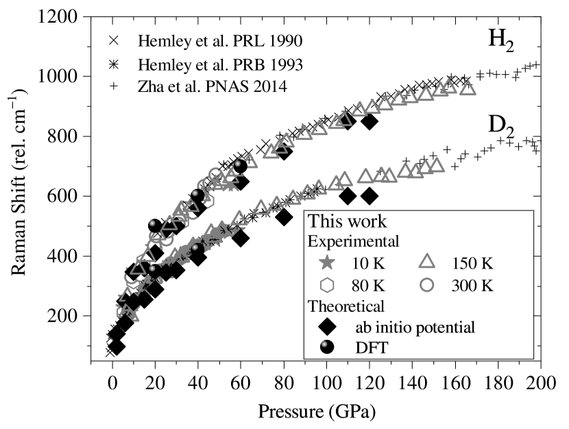
Figure 8: Comparison of previous dataHemley et al. (1990b, 1993); Zha et al. (2014) the measuredPena-Alvarez et al. (2019) and E${}_{2_{g}}$ calculated phonon modes

V Comparison with experiment

We compare our model with the results of high pressure Raman studies. Details of these experiments are given in the accompanying paperPena-Alvarez et al. (2019).

To compare with experiment, we must further assume that the equation of states are the same for hydrogen and deuterium. At relatively low pressures, below 10 GPa approximately 5% difference in specific volume and 10% in pressure has been reportedHemley et al. (1990c), but later measurements suggest the difference is smallerLoubeyre et al. (1996).

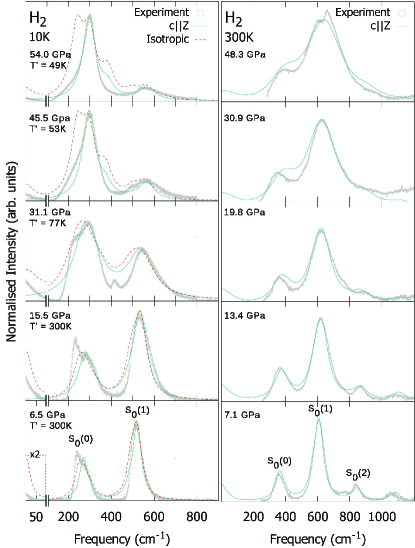
Figure 9: Theoretical Raman patterns for H₂ at selected pressures and temperatures, compared with our experimental dataPena-Alvarez et al. (2019). The pattern comprises peak positions and line-widths calculated from Eq. 35 with $\Gamma$ treated as a free parameter (see Fig. 11 and table 3 for values). Green solid line shows the predicted spectra for a sample with c axis aligned parallel to the beam, the red dashed line shows the predicted spectra in the case of a perfect powder of crystallites. $T^{\prime}$ denotes the equivalent temperature fitted to the observed $ortho-para$ ratio (see Eq. 19).

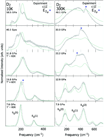
Figure 10: Theoretical Raman patterns for D₂ at selected pressures and temperatures, compared with our experimental dataPena-Alvarez et al. (2019). The model follows the same procedure for hydrogen described in the figure 9 caption with two changes. The mass is increased by a factor of 2 and the parameter $\Gamma$ from Eq. 32 is decreased by a factor of $\sqrt{2}$. The complete mismatch of theory and experiment for 10 K at high pressure indicates the experimental data is for phase II. the E${}_{2_{g}}$ phonon mode is not included in the calculated spectra

The $S_{0}(0)$ roton peak splits into three ($|\Delta M_{J}|=0,1,2)$ but this can only be reconciled with the data by noting that in a DAC experiment the crystallites have strong preferred orientation. A back-scattering geometry with the $c$-axis parallel to the beam renders the $\Delta M_{J}=1$ mode invisible (Table 2). This effect is countered by resonant scattering in which the missing $para-$ peaks are enhanced by the absorption and re-emission by the $ortho-$ modes. Previous work by Eggert et al.Eggert et al. (1999) shows that as $ortho$-H transforms over time, the shape of the $para$-roton peak changes, with the low frequency $S_{0}(0)_{1}$ peak eventually disappearing. This non-equilibrium $ortho$-$para$ ratio is described by $T^{\prime}$, which drops monotonically with time and pressure increase (see Supplemental Materials).

For comparison with experiment for hydrogen at 10 K (figure 9, left panel) two experimental geometries are considered. The green solid line shows the predicted spectra for a sample with c axis parallel to the beam. The dashed red line shows the intensities for a perfect powder. Inspection of the sample suggested that the crystallites are always oriented with the c-axis parallel to the beam as previously seen in X-ray workAkahama et al. (2010). However, whenever significant amounts of $ortho$-H are present, resonant stimulated emission means all three $S_{0}(0)$ modes have significant intensityBloembergen et al. (1967); Van Kranendonk (1983); Eggert et al. (1999).

For deuterium, experimental agreement is good at low pressures ($>$20 GPa). At higher pressures this agreement deteriorates for a number of reasons. The most glaring disagreements seen above 40 GPa at 10 K are caused by the transition to phase II. At 300 K, apparent disagreement is due to the E${}_{2_{g}}$ phonon mode which appears at similar frequencies to the $S_{0}(1)$ and $S_{2}(0)$ peaks (see blue asterisk on figure 10): the phonon is not included in the roton model. We notice a shift upwards in frequency of all modes at higher pressures which could be attributed to a shorter bond length, around 95% of the gas phase value.

Figure 11: Comparison of peak widths for hydrogen at 300 K calculated from statistical fits of Voigt profiles to experimental spectra (blue, note only $S_{0}(0)$ transitions are shown); MD trajectories with autocorrelation function (black); and single dephasing parameter fitted to entire spectrum in single molecule model (red). The autocorrelation function demonstrates surprisingly good agreement with the fitted values from experiment and the single parameter fitted to the quantum rotor model.

VI Discussion and Conclusions

We have calculated the energy levels and Raman spectra of a perturbed quantum rotor in 2 and 3 dimensions and compared directly with Raman data for high pressure hydrogen. The 2D data illustrates the isotope effect, with the ratio $\nu_{H}/\nu_{D}$ going from 2 to $\sqrt{2}$ as the perturbation becomes stronger, transforming the rotor to a harmonic oscillator. For an anharmonic oscillator, the ratio can be even lower. In 3D this is more complicated, as there are multiple degenerate minima in the potentials giving different harmonic frequencies.

The Raman spectra are calculated using two distinct approximations: in the traditional approach (see Supplememntal Materials Sec. I), transitions are identified, their Raman intensity calculated and a peakwidth is assigned to each mode. Our alternate approach sets up an excited mixed quantum state, equivalent to linear response textbook Raman theory. We then calculate the polarisation as this mixed state decays according to a single decorrelation time: Fourier transforming this yields the entire Raman spectrum. Spectra from the two approaches agree very closely (Figs. S3-S6).

A surprisingly good estimate for this decorrelation time can be extracted from the angular momentum autocorrelation function calculated using ab initio molecular dynamics with classical nuclei. Using AIMD data for $\Gamma$ and $r$ could eliminate those fitting parameters.

A good angular momentum quantum number, $J$ implies conservation of molecular angular momentum. The autocorrelation function provides a classical analogy for the concept via the decorrelation time. A good quantum number has infinite decorrelation time and decreasing decorrelation time gives a measure of the ”goodness” of the quantum number. Above 20 GPa, the decorrelation times shown in Fig. 6 are less than required for a single, full rotation, and even at low-T and 100 GPa (Fig. 7) scarcely one librational period. Thus the quantum states are well-localised, but are neither good rotors nor harmonic oscillators.

High pressure hydrogen has a Raman-active phonon mode involving movement of entire layers. This can be accurately calculated from the AIMD using the projection method (Fig. 8). It is shown to be decoupled from the rotations.

The direct comparison with the entire experimental signal revealed several issues. Most strikingly, the mean-field theory cannot be made to fit the phase II spectrum, which means that the localised-mode assumptions of the model have broken down: a conclusion also obvious from the molecular dynamics.

In summary, we have calculated the Raman signal from single-molecule quantum excited states of a perturbed rotor in a hexagonal crystal. We developed a method to directly calculate the entire spectrum with a single decorrelation parameter, which itself can be obtained from ab initio MD calculations. The transformation to the broken-symmetry phase II is clearly signalled by the failure of the theory to explain the data, while a missing peak demonstrates preferred orientation in the experimental sample.

The results support the idea that, even within phase I, the motion changes from quantum rotor to quantum libration while the mode remains localised on the molecule.