Scaling laws for the geometry of an impact-induced magma ocean

Abstract

Growing protoplanets experience a number of impacts during the accretion stage. A large impactor hits the surface of a protoplanet and produces impact-induced melt, where the impactor’s iron emulsifies and experiences metal-silicate equilibration with the mantle of the protoplanet while it descends towards the base of the melt. This process repeatedly occurs and determines the chemical compositions of both mantle and core. The partitioning is controlled by parameters such as the equilibration pressure and temperature, which are often assumed to be proportional to the pressure and temperature at the base of the melt. The pressure and temperature depend on both the depth and shape of the impact-induced melt region. A spatially confined melt region, namely a melt pool, can have a larger equilibrium pressure than a radially uniform (global) magma ocean even if their melt volumes are the same. Here, we develop scaling laws for (1) the distribution of impact-induced heat within the mantle and (2) shape of the impact-induced melt based on more than 100 smoothed particle hydrodynamic (SPH) simulations. We use Legendre polynomials to describe these scaling laws and determine their coefficients by linear regression, minimizing the error between our model and SPH simulations. The input parameters are the impact angle $\theta$ ($0^{\circ},30^{\circ},60^{\circ}$, and $90^{\circ}$), total mass $M_{T}$ ($1M_{\rm Mars}-53M_{\rm Mars}$, where $M_{\rm Mars}$ is the mass of Mars), impact velocity $v_{\rm imp}$ ($v_{\rm esc}-2v_{\rm esc}$, where $v_{\rm esc}$ is the mutual escape velocity), and impactor-to-total mass ratio $\gamma$ ($0.03-0.5$). We find that the equilibrium pressure at the base of a melt pool can be higher (up to $\approx 80\%$) than those of radially-uniform global magma ocean models. This could have a significant impact on element partitioning. These melt scaling laws are publicly available on GitHub (https://github.com/mikinakajima/MeltScalingLaw).

1 Introduction

Protoplanets experience numerous impacts as they accrete. These impacts have shaped the configuration of the solar system, given that the origins of the Earth-Moon system (e.g., Hartmann and Davis, 1975; Cameron and Ward, 1976), the Pluto-Charon system (e.g., McKinnon, 1988, 1989; Canup, 2005) and perhaps the Martian moons (e.g., Rosenblatt, 2011; Craddock, 2011; Citron et al., 2015; Rosenblatt et al., 2016; Nakajima and Canup, 2017; Canup and Salmon, 2018; Hyodo et al., 2018) can be explained by giant impacts. Additionally, the large core of Mercury (e.g., Benz et al., 2007) and Uranus’s axis tilt may have also been the result of giant impacts (e.g., Safronov, 1969; Slattery et al., 1992; Kegerreis et al., 2018).

Giant impacts are not only responsible for shaping the architecture of the planetary system, but also for determining the evolving chemistry of a protoplanet. The chemical compositions of both the mantle and core of a protoplanet evolve over time as new impactor materials are added. When an impactor hits the protoplanet (target), the outer part of the mantle becomes molten and forms a magma ocean. Some portion of the impactor’s iron core equilibrates with the ambient mantle, while the extent depends on the impactor size, velocity and impact angle (e.g., Dahl and Stevenson, 2010; Deguen et al., 2014; Landeau et al., 2016, 2021; Kendall and Melosh, 2016; Lherm and Deguen, 2018). This equilibration enriches iron melt with siderophile elements whereas lithophile elements will be preferentially partitioned into the silicate melt. The iron continues to sink to the bottom of the magma ocean and eventually merges with the target core (e.g., Stevenson, 1990; Wade and Wood, 2005; Rubie et al., 2003, 2011, 2015). However, if the impactor’s iron core is large, it may not have time to equilibrate with the target’s mantle before merging with the target’s core (Dahl and Stevenson, 2010). Thus, the extent of equilibration depends on the details of the impact process.

The metal-silicate partition coefficient of element $i$ is defined as,

$$D^{\rm metal-sil}_{i}=C_{i}^{\rm metal}/C_{i}^{\rm sil},$$ (1)

where $C_{i}^{\rm metal}$ and $C_{i}^{\rm sil}$ are the concentrations of element $i$ in metal and silicate at equilibrium, respectively (e.g., Rubie et al. 2015). This coefficient is a function of equilibrium temperature $T_{\rm eq}$ and pressure $P_{\rm eq}$ and of other factors such as the oxygen fugacity. Conventionally, the values of $T_{\rm eq}$ and $P_{\rm eq}$ are often associated with or assumed to be proportional to the values at the bottom of a magma ocean. Based on siderophile (iron-loving) elemental abundances (e.g., Ni, Co) in the Earth mantle, early partitioning studies with piston-cylinder experiments suggest that the metal-silicate equilibration occurs at $\approx 25$ GPa, while more recent studies, including higher pressure experiments with diamond anvil cells, propose up to 55 GPa (e.g., Siebert et al., 2013; Fischer et al., 2015).

Conventionally, it is assumed that such an equilibration occurs in a global (radially uniform) magma ocean of equivalent volume to the melt that is generated by the impact (Figure 1a). However, more realistically, an impact first produces a spatially confined melt pool (Figure 1b) (Tonks and Melosh, 1992; Rubie et al., 2015) that centers around the impact point. Due to isostatic adjustment this melt pool would radially spread out and become a global magma ocean over time (Reese and Solomatov, 2006), however, this timescale ($10^{2}-10^{5}$ years, Reese and Solomatov 2006) is likely to be much longer than the equilibration timescale, ranging from hours (set by the turbulent mixing timescale) to months (set by the $\approx 1$ cm-sized iron droplets’ sinking timescale suggested by Dahl and Stevenson 2010). Therefore, a melt pool is likely to be more relevant for the metal-silicate equilibration process and can provide higher pressures than a global magma ocean (Figure 1). It should be noted that the geometry and pressure differences between melt pool and magma ocean diminish when the entire mantle melts.

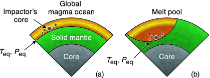
Figure 1: Schematic view of (a) a global magma ocean and (b) a regionally confined melt pool. $T_{\rm eq}$ and $P_{\rm eq}$ are the equilibrium temperatures and pressures, respectively. Even if the volumes of melt are the same between the two models, a melt pool can be deeper and reach higher $T_{\rm eq}$ and $P_{\rm eq}$ than those of a global magma ocean.

Insightful and extensive studies have been conducted to estimate the volume of an impact-induced magma ocean (e.g., Bjorkman and Holsapple, 1987; Tonks and Melosh, 1993; Pierazzo et al., 1997; Pierazzo and Melosh, 2000; Reese and Solomatov, 2006; Barr and Citron, 2011; Abramov et al., 2012; Monteux and Arkani-Hamed, 2019). However, some of these studies focus on head-on collisions (for which the impact angle $\theta$ is $0^{\circ}$; see Figure 2a for the definition of $\theta$) because the simulations of these impacts are numerically less expensive than those of oblique impacts, which require 3D simulations, even though oblique impacts are more likely (e.g., Shoemaker 1962; Agnor et al. 1999). Moreover, no detailed analytical models that describe how the heat is distributed within the mantle of the post-impact body for various impact angles are available. This renders challenging the prediction of the depth and geometry of an impact-induced melt pool.

Here, we have derived scaling laws for (1) the distribution of impact-induced heat within the mantle and (2) the geometry (shape) of the impact-induced melt. These scaling laws are expressed using Legendre polynomials and their coefficients are determined by linear regression to minimize the error between our model and impact simulations. By using these laws combined with the initial thermal profile of a planetary body, we can predict the thermal profile of the post-impact body. Moreover, once the criterion for melting is specified, the melt volume and shape of a magma ocean and melt pool can be calculated.

2 Methods

2.1 Smoothed particle hydrodynamics

We use the smoothed particle hydrodynamics (SPH) method to simulate giant impacts. SPH is a Lagrangian method and has been used for representing planetary impact phenomena (e.g., Canup 2004). All the SPH particles have the same masses in a given simulation. Each SPH particle has a characteristic length scale called smoothing length. The smoothing length becomes small when an SPH particle is surrounded by neighboring particles, while the mass of the particle remains the same. This makes the density of the particle increase at a densely populated region, whereas it decreases at a sparsely populated region. The smoothing length evolves over time, but the typical scale is $\sim 200$ km. In SPH, the conservation equations for mass, momentum, and energy are solved simultaneously. This SPH code follows the standard implementation that uses artificial viscosity to describe the shock front (see Section 4 in Monaghan, 1992). The SPH algorithm provides the density and internal energy at each time step, which are used to determine the pressure and sound velocity based on an equation of state (EOS). We use M-ANEOS as an equation of state (Thompson and Lauson, 1972; Melosh, 2007), which is a semi-analytic equation of state and includes phase changes. This equation of state has been frequently used in previous impact simulations (e.g., Canup, 2004). The input parameters for M-ANEOS are listed in Supplementary Information (our input file is listed as “SPH-N” in Stewart et al. 2020). This version of M-ANEOS does not include the effect of melting, and therefore it overestimates the temperature of a material that is heated above the melting point. The mantle and core are assumed to be dunite and iron, respectively. The initial mantle mass fractions $f_{\rm mantle}$ for both impactor and target are 0.7 (i.e. the core mass fractions are 0.3). Initially, the mantle and core of a body have adiabatic temperature profiles. The entropies for the mantle and core are assumed to be 3160 J/K/kg and 1500 J/K/kg, respectively, which results in approximately $\approx 2000$ K near the planetary surface and $\approx 4000$ K in the iron core at the core mantle boundary (CMB) for an Earth-sized planet. Effects of varying the initial temperatures are considered in Section 3.4. The number of SPH particles in our simulations is on the order of $10^{4}-10^{5}$, as discussed in more detail in Section 4.5. The initial locations and velocities of the impactor and target are calculated as follows; (1) determining the locations and velocities of the target and impactor upon impact with the desired impact angle and velocity, and (2) calculating the trajectories of the two bodies backwards in time until the two bodies are apart by 2 Earth radii (we define this state as $t=0$ where $t$ is time). In this backward trajectory calculation, tidal deformation is ignored. For this reason, the impact angle and velocity in an SPH simulation can be slightly different from the desired values due to tidal deformation prior to the impact, but we assume that this effect is minor and it is meritorious to capture pre-impact tidal deformation because this contributes to heating. Our SPH code does not include material strength and the implication of this omission is discussed in Section 4.4. The details of the code and settings are described in detail in our previous studies (e.g., Nakajima and Stevenson, 2014, 2015).

2.2 Parameters for the SPH simulations

The input parameters for the SPH simulations are the impact angle $\theta$ ($0-90^{\rm o}$, Figure 2a), total mass $M_{T}$ ($1M_{\rm Mars}-53M_{\rm Mars}$, where $M_{\rm Mars}$ is the mass of Mars), which is the sum of target and impactor masses, the impactor-to-total-mass ratio $\gamma$ ($0.03-0.5$), impact velocity $v_{\rm imp}$ ($v_{\rm esc}-2v_{\rm esc}$), where $v_{\rm esc}$ is the mutual escape velocity ($v_{\rm esc}=\sqrt{2G(M_{t}+M_{i})/(R_{t}+R_{i})}$, where $G$, $M_{t}$, $M_{i}$, $R_{t}$, $R_{i}$ are the gravitational constant, target mass, impactor mass, target radius and impactor radius). The values of the employed parameters are listed in Table 1 and input parameters are listed in Tables S.1 - S.3. Impacts with parameters in these ranges are expected to be common near the end of the planetary accretion stage (e.g., Ward, 1993; Agnor et al., 1999; Agnor and Asphaug, 2004), when the impacts are largest and have the greatest influence on planetary composition. Figure S.1 shows the distributions of these parameters in previous orbital evolution calculations (Rubie et al., 2015), where the typical ranges are $30^{\circ}\leq\theta\leq 60^{\circ}$, $M_{T}\leq 1-2M_{\rm Mars}$, $v_{\rm imp}\leq 1.5v_{\rm esc}$, and $\gamma\leq 0.05$.

Symbol	Description	values	references
$\theta$	Impact angle	0-90∘
$M_{T}$	Total mass	1 - 53 $M_{\rm Mars}$
$\gamma$	Impactor-to-total-mass ratio	$0.03-0.5$
$M_{\rm Mars}$	Martian mass	$6.4171\times 10^{23}$ kg
$M_{t}$	Target mass	$(1-\gamma)M_{T}$
$M_{i}$	Impactor mass	$\gamma M_{T}$
$R_{t}$	Target radius	$1-3R_{\rm Mars}$
$R_{i}$	Impactor radius	$0.5-1.5R_{\rm Mars}$
$R^{{}^{\prime}}$	Radius of a planet whose mass is $M_{t}+M_{i}$	$1-3R_{\rm Mars}$
$v_{\rm imp}$	Impact velocity	$v_{\rm esc}$ - 2 $v_{\rm esc}$
$v_{\rm esc}$	Mutual escape velocity	$4.2-17.5$ km/s
$M_{\rm mantle}$	Post-impact mantle mass	$0.5-1.0M_{T}$
$h$	Mantle heating/total heating	$0.7-1.0$
$E_{M}$	Specific energy for melting	$5.2\times 10^{6}$ J/kg	1
$\Delta IE$	Internal energy gain	$10^{29}-10^{32}$ J	2
$KE_{0}$	Kinetic energy	$10^{29}-10^{32}$ J
$\Delta PE$	Change in potential energy	$10^{29}-10^{32}$ J
$c_{v}$	Specific heat	1000 J/K/kg	3
$f_{\rm mantle}$	Initial mantle mass fraction	0.7
$dE_{\rm mantle}/dE$	Fractional heating of mantle	0.6-1

Table 1: List of key parameters used in this paper. 1: Pierazzoetal1997, 2: Equation 4, 3: Estimated from M-ANEOS.

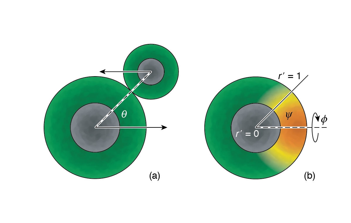
Figure 2: Definition of our model parameters. (a) $\theta$ is the impact angle, where the arrows indicate the directions of motions of the impactor and the target. (b) The polar angle $\psi$ is defined to be zero where the shock-heating is most significant, which is typically close to the impact point. The heat distribution is assumed to be symmetric along the $\psi=0$ axis and therefore its dependence on the azimuth angle $\phi$ is ignored. $r^{\prime}$ is the normalized radius of the post-impact body (0 is the center of the body and 1 is its surface).

3 Scaling law of mantle melt and heat distribution

The SPH results are listed in Tables S.1-S.2 for the $v_{\rm imp}=v_{\rm esc}$ cases and in Table S.3 for the $v_{\rm imp}\geq 1.1v_{\rm esc}$ cases. The model name “M” represents the same set of initial conditions with four different impact angles (in the range of $\theta=0^{\circ}-90^{\circ}$). ID represents a specific SPH simulation. $dE$ is the total internal energy gain of the post-impact body, $dE_{\rm mantle}/dE$ represent the fraction of the internal energy partitioned into the mantle (i.e. $1-dE_{\rm mantle}/dE$ is the fractional energy partitioned into the core). $M_{\rm mantle}/(f_{\rm mantle}M_{T})$ represents the extent of perfect or imperfect accretion of the mantle materials (if this value is close to 1, the impactor’s mantle accretes into the target almost perfectly, whereas if this value is smaller than 1, some mass does not accrete into the post-impact body). The underlying assumption here is that the mantle mass fraction of the post-impact body is close to the original value, 0.7. This is an reasonable assumption in the parameter ranges we explore, but it may not be accurate if the impact velocity is much larger and the impact is catastrophic enough to change the fraction (e.g., Benz et al., 2007). $MF_{A}$ is the melt mass fractions of the post-impact body based on the melt criterion discussed in Section 3.3 (Equation 13). $\sigma^{\prime}$ refers to the error between an SPH simulation and our model (see Section 3.3). $N$ is the number of SPH particles. Additional outputs are discussed in Section S.2.

We describe the results of our model in terms of (1) the internal energy gain by impact in Section 3.1 and (2) heat distribution within the mantle in Section 3.2. By combining these two sets of results, the internal energy gain and geometry of melt can be modeled as discussed in Section 3.3.

3.1 Impact-induced heating

3.1.1 SPH simulations

Examples of our SPH simulations are presented in Figure 3 (model M0). The orange-red color map displays the gain of specific internal energy of the mantle normalized by $10^{5}$ J/kg and the grey color applies to iron. These snapshots clearly show that the internal energy gain depends on the impact angle $\theta$. For a head-on collision ($\theta=0^{\circ}$), antipodal heating is prominent due to focusing of shock waves at the opposite side of the impact point and due to deformation of the mantle. Part of the mantle at the antipode deforms significantly and expands radially upon impact. When it falls back and hits the core mantle boundary, the potential energy is converted into internal energy of the mantle. This effect is stronger at $\theta=0^{\circ}$ and is not clearly observed at other angles. At $\theta=30^{\circ}$, an impactor accretes onto the target and heats the mantle near the impact site. At $\theta=60^{\circ}$, the impactor hits the target twice; during the first impact, only a small portion of the impactor accretes onto the target, whereas the rest of the impactor accretes onto the target during the second impact (the so-called “graze-and-merge collisions”). The target mantle is more uniformly heated at this impact angle (at $\theta=60^{\circ}$ in Figure 3). The target’s iron becomes more fragmented during the impact process. This effect is not considered in our melt model as discussed in the following sections, but it is an important effect given that this would lead to a higher extent of metal-silicate mixing compared to cases where the core is nearly intact. At $\theta=90^{\circ}$, the impactor grazes the target mantle and does not accrete onto the target. Consequently, only a small portion of the target is heated.

3.1.2 Analytical models for $KE_{0}$ and $\Delta PE$

As a first step for describing the total internal energy gain $\Delta IE$, we describe the initial kinetic energy of the system $KE_{0}$ as

$$KE_{0}=\frac{1}{2}\frac{M_{t}M_{i}}{M_{t}+M_{i}}v_{\rm imp}^{2}.$$ (2)

Assuming perfect accretion and ignoring any shape change of the post-impact body due to rotation and heating, the gain of the potential energy due to an impact, $\Delta PE$, is expressed as

$$\Delta PE=-\frac{3}{5}\frac{GM_{t}^{2}}{R_{t}}-\frac{3}{5}\frac{GM_{i}^{2}}{R_{i}}-\frac{GM_{t}M_{i}}{R_{t}+R_{i}}+\frac{3}{5}\frac{G(M_{t}+M_{i})^{2}}{R^{\prime}},$$ (3)

where $R^{\prime}$ represents the radius of a body whose mass is $M_{t}+M_{i}(=M_{T})$ (the mass-radius relationship between $M_{T}$ and $R^{\prime}$ is described in Section S.1). The first and second terms are the gravitational binding energies of the target and impactor bodies. The third term represents the gravitational energy of the impactor body in the gravity potential of the target body, and the fourth term is the gravitational binding energy of the post-impact body under the assumption that the target and impactor perfectly merge. Equation 3 is an idealized potential energy gain assuming a perfect accretion event. The actual potential energy release can differ from this because some mass can be lost and the mass-radius relationship can change due to the temperature profile and spin of the body (see Section S.2). Moreover, this expression does not include the effect of differentiation, which could account for up to $\sim 10\%$ of internal energy increase (Stevenson , D. J., online textbook). Nevertheless, $\Delta PE$ still gives a first order estimate for the potential energy change after a merging impact.

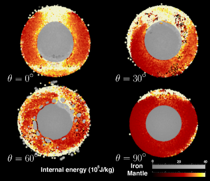
Figure 3: Examples of SPH simulations (Model series M0 - see Table 2. $M_{T}=1M_{\rm Mars},\gamma=0.1,v_{\rm imp}=v_{\rm esc}$). The four panels show the results for different impact angles approximately 20 hours after the impacts. The grey and red-orange colors represent the internal energy of the iron core and silicate mantle, respectively (the values are shown in $10^{5}$ J/kg). $\psi=0^{\circ}$ is placed in the direction of 12 o’clock. The internal energy gain strongly depends on the impact angle.

3.1.3 Fitting models for $\Delta IE$, the mantle mass, and the fractional heating

We assume that the total internal energy gain $\Delta IE$ is a function of $\Delta PE$ and $KE_{0}$, and is expressed by the Legendre polynomials $P_{l}$ as

$$\Delta IE(\theta)=(KE_{0}+\Delta PE)\sum_{l=0}^{n_{e}}e_{l}P_{l}(\cos\theta),$$ (4)

where $e_{l}$ are the corresponding coefficients (see Tables S.5-S.6) and $n_{e}$ is the order of the polynomial. The scaled internal energy gain $\Delta IE/(KE_{0}+\Delta PE)$ can exceed 1 because $\Delta PE$ is an simplified energy estimate as discussed in Section 3.1.2. In Figure 4a, b, our best fit model is shown as a thick black line, which is modeled by sixth order Legendre polynomials ($n_{e}=6$). The lines with colors represent $\Delta IE_{\rm SPH}/(KE_{0}+\Delta PE)$, where $\Delta IE_{\rm SPH}$ is the internal energy gains calculated from SPH simulations. The left and right panels represent the $v_{\rm imp}=v_{\rm esc}$ and the $v_{\rm imp}\geq 1.1v_{\rm esc}$ cases, respectively. The coefficients $e_{l}$ are determined by minimizing the error $\sigma$ (linear regression),

$$\sigma=\sqrt{\frac{1}{n}\sum_{i=1}^{n}\left(\frac{\Delta IE_{{\rm SPH},i}-\Delta IE_{i}}{KE_{0}+\Delta PE}\right)^{2}},$$ (5)

where $\Delta IE_{{\rm SPH},i}$ is the internal energy gain from an SPH simulation whose ID is $i$ and $\Delta IE_{i}$ is the internal energy gain estimated with Equation (4) for ID$=i$. $n$ is the total number of simulations we consider ($n=64$ is for $v_{\rm imp}=v_{\rm esc}$ and $n=44$ for $v_{\rm imp}\geq 1.1v_{\rm esc}$). The colors of the lines represent different $\gamma$ values (for details, see the figure caption). The scaled internal energy gain $\Delta IE/(KE_{0}+\Delta PE)$ at $v_{\rm imp}=v_{\rm esc}$ is typically larger than that at $v_{\rm imp}\geq 1.1v_{\rm esc}$. This is because impacts at $v_{\rm imp}=v_{\rm esc}$ result in nearly perfect mergers, which can efficiently convert the impact kinetic energy and potential energy into internal energy; however, this does not always hold for cases with higher impact velocities ($v_{\rm imp}\geq 1.1v_{\rm esc}$), which often result in hit-and-run collisions especially at large impact angles ($\theta=60^{\circ},90^{\circ}$) (e.g., Asphaug 2009; Genda et al. 2012). This scaled internal energy gain decreases as the impact angle increases for the same reason; at large impact angles, the kinetic and potential energies are not efficiently converted into internal energy.

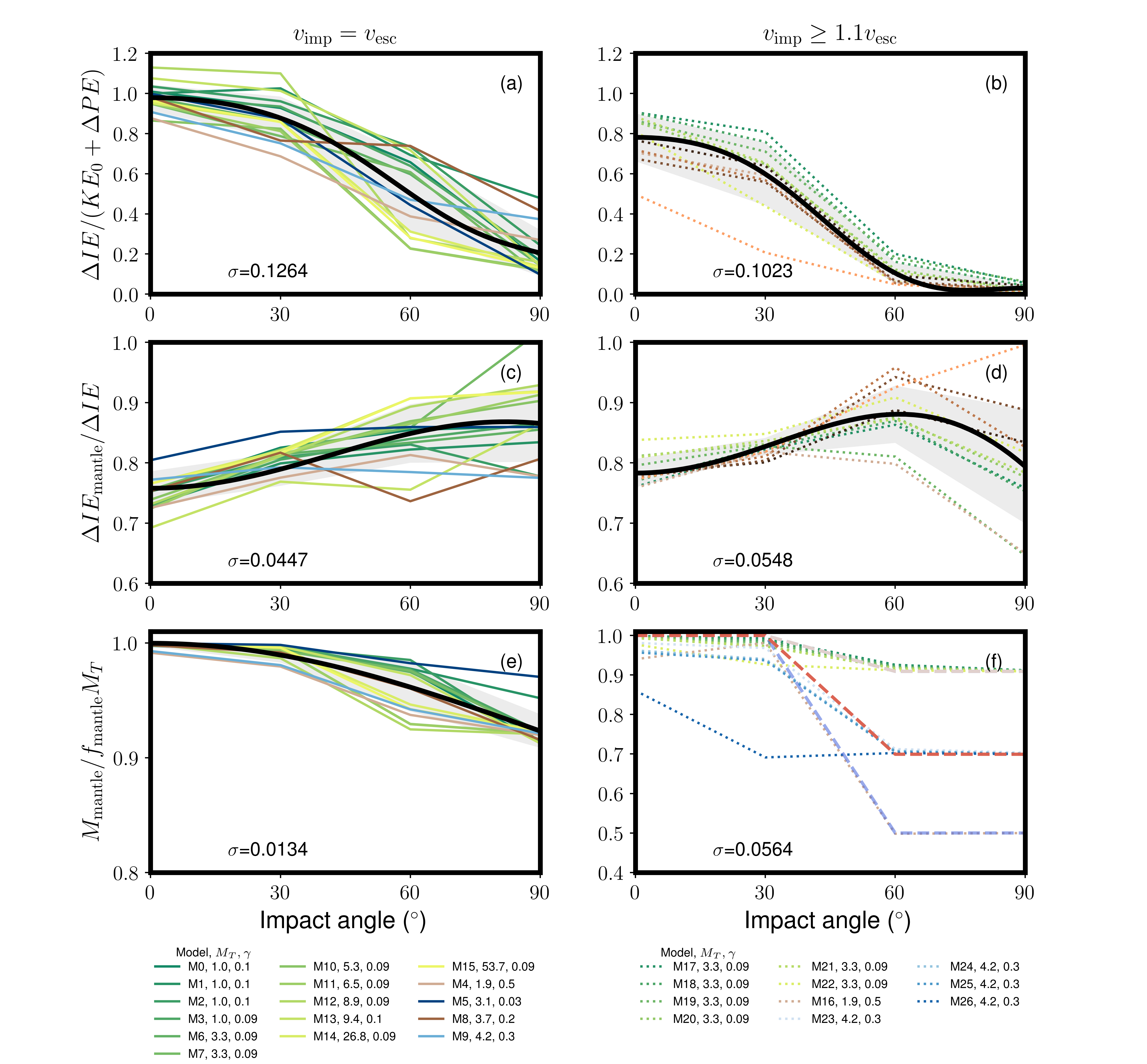
Figure 4: The left panels correspond to the $v_{\rm imp}=v_{\rm esc}$ cases and the right panels correspond to the $v_{\rm imp}\geq 1.1v_{\rm esc}$ cases. The empirical fits are shown with the thick black lines in panels a-e and dashed lines in panel f. SPH calculations are shown with the solid lines for the $v_{\rm imp}=v_{\rm esc}$ cases and dotted lines for the $v_{\rm imp}\geq 1.1v_{\rm esc}$ cases. (a, b) The total internal energy gain normalized by the sum of the initial kinetic energy $KE_{0}$ and $\Delta PE$. The colors of the solid lines represent $\gamma$ values; green-yellow lines (M0-M3, M6-M7, M10-M15, M17-M22) for $\gamma=0.09-0.1$, light brown (M4, M16) for $\gamma=0.5$, blue (M5) for $0.03$, brown (M8) for $0.2$, skyblue (M9, M23-M26) for $\gamma=0.3$. (c, d) The fractional heating of the mantle with respect to the total heating. (e) $M_{\rm mantle}/f_{\rm mantle}M_{T}$ represent the extent of perfect or imperfect accretion at $v_{\rm imp}=v_{\rm esc}$. (f) Same as (e) but at $v_{\rm imp}\geq 1.1v_{\rm esc}$. The dashed lines represent Equation 8. The legend names correspond to the models listed in Tables S.1-S.3. The standard deviation $\sigma$ is listed in each panel (Equation 5) and the grey shadow represents the error envelope in panels (a-e).

In Figure 4c, d, the fractional heating of the mantle with respect to the total internal energy gain, $\Delta IE_{\rm mantle}/\Delta IE$ is shown as a function of the impact angle. The fitting model $h(\theta)$ for this parameter at $v_{\rm imp}=v_{\rm esc}$ is expressed as

$$h(\theta)=\sum_{l=0}^{n_{g}}g_{l}P_{l}(\cos\theta),$$ (6)

where the coefficients $g_{l}$ are listed in Tables S.5 and S.6 ($n_{g}=2$). $h(\theta)$ generally increases at larger impact angles for the following reasons: an impact at a small impact angle is energetic enough to heat the core in addition to the mantle, whereas an impact at a larger impact angle tends to heat only the mantle and it is not energetic enough to heat the core. This effect can also be seen in Figure 3, where the core is shock heated at $\theta=0^{\circ}$, whereas almost no strong heating occurs at $\theta=90^{\circ}$.

The mass of a post-impact body resulting at $v_{\rm imp}=v_{\rm esc}$ is modeled as (Figure 4e)

$$M_{\rm mantle}(\theta)=f_{\rm mantle}(M_{t}+M_{i})\sum_{l=0}^{n_{k}}k_{l}P_{l}(\cos\theta),$$ (7)

where $n_{k}=1$ and the coefficients $k_{l}$ are listed in Table S.5. The best fit is shown with the thick black line in Figure 4c and the corresponding coefficients $k_{l}$ are listed in Table S.5 ($n_{k}$ = 1). At $\theta=0^{\circ}$, a target and an impactor perfectly accrete, but up to $\approx 10\%$ of the total mass, $M_{T}$, does not accrete at $\theta=90^{\circ}$ (Figure 4). At $v_{\rm imp}\geq 1.1v_{\rm esc}$, the mantle mass of a post-impact body is not well captured by Equation 7, which assumes almost perfect accretion, because high velocity impacts tend to result in hit-and-run collisions. At $v_{\rm imp}\geq 1.1v_{\rm esc}$, we use the following simple imperfect accretion model (shown with the dashed lines in Figure 4f),

$$M_{\rm mantle}(\theta)=\begin{cases}f_{\rm mantle}(M_{t}+M_{i}),&\text{at}\ 0^{\circ}\leq\theta\leq 30^{\circ}\\ f_{\rm mantle}[M_{t}-M_{i}(\frac{\theta}{30}-2)],&\text{at}\ 30^{\circ}<\theta\leq 60^{\circ}\\ f_{\rm mantle}M_{t},&\text{at}\ 60^{\circ}<\theta\leq 90^{\circ}.\\ \end{cases}$$ (8)

It should be noted that at $v_{\rm imp}=v_{\rm esc}$ and $\theta=90^{\circ}$, our scaled internal energy model (Equation 4) is underestimated in some cases. An impactor hits the surface of the target and continues to orbit around the target and eventually hits the target again. However, some of the SPH simulations are stopped before an impactor comes back because we only run simulations up until $\approx 20-25$ hours, when the effect of numerical viscosity becomes non-negligible (Canup, 2004). This can be seen in Figure 4e, where some impactors accrete into targets while others do not (e.g., Models M10 and M11). We expect that this could lead to up to $\approx 10\%$ error in the internal energy given that the standard deviation at $\theta=90^{\circ}$ is 0.115 (see the grey error envelope in Figure 4a).

3.2 Distribution of heat

The heat distribution within a planetary mantle is also modeled with Legendre polynomials. We define the spatial heat distribution function $F(r^{\prime},\psi,\phi)$ as

$$F(r^{\prime},\psi,\phi)=F(r^{\prime},\psi)\equiv\frac{\Delta U(r^{\prime},\psi)}{\Delta\bar{U}},$$ (9)

where $r^{\prime}$ is the normalized radius (0 at the center and 1 at the planetary surface), $\psi$ is the colatitude, and $\phi$ is the azimuth (see Figure 2b). We assume that the heat distribution is symmetric along the pole and therefore the model does not depend on $\phi$. This assumption is not accurate when $\theta>0^{\circ}$. Nevertheless, this angle dependence is relatively weak, so we ignore it in this model (see Section S.1 and Figure S.2 for further discussion). $\psi$ is defined as zero where the impact-induced heating is maximum, which often coincides with the impact point. $\Delta U(r^{\prime},\psi)$ is the specific internal energy gain at $r^{\prime}$ and $\psi$. $\Delta\bar{U}$ is the average specific internal energy gain of the mantle. Here, $F(r^{\prime},\psi)$ is assumed to be

$$F(r^{\prime},\psi)=\sum_{m=-2}^{2}\sum_{l=0}^{2}c_{l+3(m+2)}r^{\prime m}P_{l}(\cos\psi).$$ (10)

This expression requires $5\times 3=15$ coefficients $c$, which are determined as follows. We divide an SPH simulation output into $8\times 12$ segments as a function of radius and angle, $r^{\prime}_{i}-\frac{1}{2}\Delta r\leq r^{\prime}<r_{i}^{\prime}+\frac{1}{2}\Delta r^{\prime}$ and $\psi_{j}-\frac{1}{2}\Delta\psi\leq\psi<\psi_{j}+\frac{1}{2}\Delta\psi$ ($\Delta r^{\prime}\approx 0.5/8=0.0625$ and $\Delta\psi=180^{\circ}/6=30^{\circ}$). For this, we calculate the average of $\Delta U(r^{\prime},\psi)/\Delta\bar{U}$ of the hemisphere at each segment (one hemisphere covers $-90^{\circ}\leq\phi<90^{\circ}$ and the other covers $90^{\circ}\leq\phi<270^{\circ}$, where $\phi=0^{\circ}$ and $\phi=180^{\circ}$ are parallel to the impact velocity vector). To define the location of $\psi=0$, we calculate the averaged internal energy gain at each $\psi$ segment ($\psi_{j}-\frac{1}{2}\Delta\psi\leq\psi<\psi_{j}+\frac{1}{2}\Delta\psi$ and $0.55\leq r^{\prime}<1$), and we identify $\psi$ at which the internal energy gain is maximum and set it as $\psi=0$. The 15 coefficients in Equation 10 are determined by minimizing the error between the model and the averaged internal energies in all the segments (the 15 coefficients are listed in Table S.7). It should be noted that the coefficients are determined using all the SPH simulations, including both the $v_{\rm imp}=v_{\rm esc}$ and $v_{\rm imp}\geq 1.1v_{\rm esc}$ cases. We also explored different orders ($r^{\prime-3},r^{\prime 3},P_{3}(\cos\psi)$), but their effects were limited and therefore we did not include these terms in the model.

$F(r^{\prime},\psi)$ is shown in Figure 5. The antipodal heating is well captured at $\theta=0^{\circ}$, which is not clearly seen in the case of the other impact angles. Interestingly, the mantle is heated more uniformly at small impact angles ($\theta=0^{\circ},30^{\circ}$) than at larger impact angles ($\theta=60^{\circ},90^{\circ}$). This finding may seem counter-intuitive, but this can be explained given that an impact with a small impact angle often results in accretion, which is an efficient way to heat the whole mantle, whereas an impact with a large angle heats only the near surface regions of the target body.

Figure 5: Normalized heat distribution model $F(r^{\prime},\psi)$ (Equation 10) for four different impact angles. The internal energy is normalized by the averaged energy of the system. The error is calculated at each impact angle.

3.3 Comparison between our heat distribution model and SPH

$\Delta\bar{U}$ (Equation 9) is calculated by averaging the internal energy gains of SPH particles. We assume that $\Delta\bar{U}\approx\Delta IE(\theta)$ where $\Delta IE(\theta)$ is a model fit (Equation 4). This leads to

$$\Delta U(r^{\prime},\psi,\theta)=F(r^{\prime},\psi)\Delta IE(\theta).$$ (11)

Figures 6 and 7 show the internal energy gains calculated from the SPH simulations (left) and model $\Delta U$ (right) for the models $M0$ and $M17$, respectively. Here, the internal energy gain is normalized by $10^{5}$ J/kg. The standard deviation $\sigma^{\prime}$ is described as

$$\sigma^{\prime}=\sqrt{\sum_{i=1}^{n_{r^{\prime}}}\sum_{j=1}^{n_{\psi}}\frac{1}{n_{r^{\prime}}n_{\psi}}\left[\Delta IE_{\rm SPH}(r^{\prime}_{i},\psi_{j})-\Delta IE(r^{\prime}_{i},\psi_{j})\right]^{2}},$$ (12)

where $n_{r^{\prime}}=8$ and $n_{\psi}=12$. In general, the overall trend is captured in our model; at $\theta=0^{\circ}$, the mantle is extensively heated near the impact and antipodal site, whereas the mantle remains colder at $\psi=90^{\circ}$ and $-90^{\circ}$. At $\theta=30^{\circ}$, the mantle on the hemisphere close to the impact ($|\psi|<90^{\circ}$) is significantly heated, whereas the other side of the hemisphere ($90^{\circ}<|\psi|<180^{\circ}$) is much less shock-heated. At $\theta=60^{\circ}$ for M0, a portion of the mantle near the core mantle boundary is highly shock heated in the SPH simulation. This is because part of the mantle is locally heated while the impactor’s core sinks to the bottom. This is not captured in the model. At $\theta=90^{\circ}$, our model underestimates impact-induced heating in models M0 and M17 primarily because our $\Delta IE$ model also underestimates heating (Figure 4 a,b). Our model works well at small $\gamma$, but it does not work as well at $\gamma=0.5$ where an impactor is as large as the target (Figure S.7). This is because this impact is more energetic than cases with smaller $\gamma$ and our model underestimates the extent of heating.

Figure 6: Comparison between SPH results (left) for M0 model series (Table S.1) and the scaling law (right) for (top row) $\theta=0^{\circ}$, (second row) $30^{\circ}$, (third row) $60^{\circ}$, (bottom row) $90^{\circ}$, respectively. The input parameters are $M_{T}=1M_{\rm Mars},\gamma=0.1,v_{\rm imp}=v_{\rm esc}$. The color contour represents the internal energy normalized by $10^{5}$ J/kg after the system reaches its equilibrium (typically within 10 hours). The heat distribution of the mantle based on the SPH simulation is not smooth at several places partly because SPH data are segmented and partly because the internal energy, especially near the core-mantle boundary, is smaller than the contour intervals. The standard deviation $\sigma^{\prime}$ is also normalized by $10^{5}$ J/kg.

Figure 7: SPH results for model M17 (Table S.3). The color scheme is the same as the one in Figure 6. The input parameters are $M_{T}=3.25M_{\rm Mars},\gamma=0.091,v_{\rm imp}=1.2v_{\rm esc}$. The standard deviation $\sigma^{\prime}$ is normalized by $10^{5}$ J/kg.

3.4 Effect of the initial temperature

In this section, we explore the geometry of a magma ocean by considering two different initial temperature profiles of the mantle. In Figure 8, the panels (a) and (c) represent the total internal energy and the panels (b) and (d) represent the melt fraction for M0 at $\theta=0^{\circ}$. The pre-impact mantle entropy $S_{0}$ is 1100 J/K/kg for (a) and (b) (the surface temperature of $\approx 300$ K) and 3160 J/K/kg for (c) and (d) (the surface temperature of $\approx 2000$ K). These isentropic temperature profiles are calculated using M-ANEOS (see Section S.1). The total internal energy is calculated as the sum of the initial internal energy and internal energy gain using Equation 11. We define a portion of the mantle is molten if the local temperature exceeds the melting temperature, $T_{\rm melt}$ (Rubie et al., 2015),

$$P\leq 24\ {\rm GPa}:T_{\rm melt}{\rm[K]}=1874+55.43P-1.74P^{2}$$

$$+0.0193P^{3}$$

$$P>24\ {\rm GPa}:T_{\rm melt}{\rm[K]}=1249+58.28P-0.395P^{2}$$

$$+0.0011P^{3},$$ (13)

where $P$ is the pressure in GPa. The local temperature is calculated assuming $u=c_{v}T$, where $c_{v}$ is the specific heat and $T$ is the temperature. In panels (b) and (d), the yellow regions represent melt and black regions represent solid mantle. Pressure is calculated with M-ANEOS assuming that the planet is in a hydrostatic equilibrium and isentropic. No partial melting is considered. As shown in Figure 8, different initial temperatures affect not only the melt volume, but also the shape of the melt. In panel (b), the melt pool is confined to one hemisphere ($|\psi|<90^{\circ}$), whereas the melt volume is larger in panel (d) and the melt is globally distributed. It should be noted that the M-ANEOS used here does not consider solid-liquid transition and therefore this criterion overestimates the melt volume.

Figure 8: Effect of initial temperature is considered for model M0 at $\theta=60^{\circ}$. (a) Total internal energy assuming initial entropy $S_{0}=1100$ J/K/kg (this corresponds to a surface temperature of $\approx 300$ K). The total internal energy is calculated as a summation of the pre-impact internal energy and the internal energy gain calculated in Equation 11. (b) Melt mass fraction. When the mantle temperature is above the melt temperature, this value is 1, otherwise the value is 0 (no partial melting is considered). (c) is the same as (a) except $S_{0}=3160$ J/K/kg (this corresponds to a surface temperature of $\approx 2000$ K). (d) is the same as (b) except $S_{0}=3160$ J/K/kg.

3.5 Magma ocean depth and the corresponding pressure

Figure 9a-f shows the pressures at the base of (1) a melt pool (panels a-b), (2) a global magma ocean (panels c-d), and (3) a global magma ocean whose melt volume is estimated by a bulk heating model (panels e-f) as discussed below for all $v_{\rm imp}=v_{\rm esc}$ cases. The left panels correspond to the $S_{0}=1100$ J/K/kg cases and the right panels correspond to the $S_{0}=3160$ J/K/kg cases. The shaded regions represent the error envelopes. In the melt pool model, we calculate its shape as discussed in Section 3.4. The pressure at the deepest portion of the melt pool is defined as $P_{\rm Melt\ pool}$. In the global magma ocean model, the melt volume is the same as that of the melt pool, whereas the magma ocean depth is uniform (Figure 1a) and the pressure at the base of the magma ocean is defined as $P_{\rm Global\ MO}$. In the bulk heating model, the melt mass fraction of the mantle, $f_{\rm melt}$, is described as

$$f_{\rm melt}=\frac{h(\theta)\Delta IE(\theta)}{M_{\rm mantle}(\theta)E_{M}},$$ (14)

where $E_{M}$ is the specific energy required for the material to melt after it experiences isentropic decompression down to 1 atm (Bjorkman and Holsapple, 1987). Criteria of this type have been widely used in previous studies (e.g., Abramov et al. 2012; Pierazzo and Melosh 2000). $P_{\rm Bulk\ heating}$ is defined as the pressure at the bottom of a magma ocean whose melt volume is $f_{\rm mantle}\frac{4\pi}{3}(R_{p}^{3}-R_{c}^{3})$, where $R_{p}$ is the radius and $R_{c}$ is the core radius of the post-impact body. Figure 9g and h represent the fractional difference in pressure between the melt pool model and global magma ocean model, $\Delta P/P_{\rm Melt\ pool}$, where $\Delta P=|P_{\rm Melt\ pool}-P_{\rm Global\ MO}|$. The error envelopes are excluded in f-g panels.

As shown in the figure, $P_{\rm Melt\ pool}$ is usually greater than $P_{\rm Global\ MO}$, unless the entire mantle is molten. Higher $S_{0}$ causes forming deeper magma oceans as also seen in Figure 8. Comparison between the bulk heating model and the other models is not straightforward because the depth of a magma ocean critically depends on the value of $E_{M}$, which is not well constrained. The fractional difference between $P_{\rm Melt\ pool}$ and $P_{\rm Global\ MO}$ can range from 0 to $\approx 0.8$ (panels g and h). The difference tends to be large at $\theta=90^{\circ}$, where the melt volume is smaller than those at the other angles and the geometry of a melt affects the pressure at the base of the melt region.

Figure 9: The pressures at the bottom of melt for the $v_{\rm imp}=v_{\rm esc}$ cases. The left panels represent the initial mantle entropy of $S_{0}=1100$ J/K/kg, and the right panels represent $S_{0}=3160$ J/K/kg. (a, b) The pressure at the base of a melt pool, $P_{\rm Melt\ pool}$, (c, d) pressure at the base of a global magma ocean $P_{\rm Global\ MO}$, and (e, f) pressure of a melt whose volume is calculated from the bulk heating model, $P_{\rm Bulk\ heating}$ (see the main text), which does not depend on the initial temperature profile, and (g, h) the fractional difference in pressure between the melt pool and global magma ocean model ($\Delta P/P_{\rm Melt\ pool}=|P_{\rm Melt\ pool}-P_{\rm Global\ MO}|/P_{\rm Melt\ pool}$). The shaded regions in (a-f) show the error envelopes.

4 Discussion

4.1 Python script for the melt scaling laws on GitHub

We provide a Python script for this model on GitHub. In this script, $\Delta IE(\theta)$ is computed based on the fitting model we develop (Equation 4) as a function of the impact angle $\theta$, total mass $M_{T}$, impactor-to-total mass ratio $\gamma$, and impact velocity $v_{\rm imp}$. The options for the impact angle $\theta$ are $0^{\circ},30^{\circ},60^{\circ}$, and $90^{\circ}$, but we intend to include $45^{\circ}$ in the near future. Users can choose one of the options which is closest to the desired impact angle. Alternatively, users can interpolate the impact angles, but such interpolation has not been tested in this work. Impact-induced heating is modeled using Equation 11. The initial thermal state of the mantle can be selected from the following options; (a) $S_{0}=1100$ J/K/kg, and (b) $S_{0}=3160$ J/K/kg, but in the future we are planning to add more options. So far we calculate the shape of a magma ocean as well as the pressure at the base of the melt using the melt criterion from Rubieetal2015, but users can easily modify this criterion if necessary.

Our simulations do not include cases at $v_{\rm esc}<v_{\rm imp}<1.1v_{\rm esc}$, which is a common impact velocity range at the end of the planetary accretion phase (see Figure S.1). To take this into account, in the Python script, we use $v_{\rm cr}$, which is the critical velocity above which the target and impactor do not merge, as derived in Gendaetal2012,

$$\frac{v_{\rm cr}}{v_{\rm esc}}=d_{1}\Gamma^{2}\Theta^{d_{5}}+d_{2}\Gamma+d_{3}\Theta^{d_{5}}+d_{4},$$ (15)

where $\Gamma=(M_{t}-M_{i})/M_{T}$ and $\Theta=1-\sin\theta$, $d_{1}=2.43,d_{2}=-0.0408,d_{3}=1.86,d_{4}=1.08,d_{5}=5/2$. When $v_{\rm imp}\leq v_{\rm cr}$, the low velocity parameters ($v_{\rm imp}=v_{\rm esc}$) are used, whereas when $v_{\rm imp}>v_{\rm cr}$, the high velocity parameters ($v_{\rm imp}\geq 1.1v_{\rm esc}$) are used.

4.2 Model simplifications

Our SPH simulations take into account the latent heat of silicate vaporization, but the effect is not explicitly considered in our analytical melt model. In most of our simulations, the vapor mass fractions (VMFs) are small ($<0.1$), but in some energetic cases, VMFs are large (0.1-1.0). In these cases, it is likely that the majority of the post-impact mantle experiences melting, and therefore a detailed melt scaling law may not be necessary when vaporization matters (see Section S.2 for detailed discussion).

In our scaling law, we assume that the initial temperature profile of a planet does not affect the internal energy gain. For this reason, the total internal energy after an impact is calculated by simply adding an initial internal energy and internal energy gain obtained from our model. This is probably a fine assumption given that small changes in the internal energy do not affect the overall structure of a planet (such as the mass-radius relationship). We also ignore the heating dependence on the azimuth ($\phi$) for simplicity. This should be fine for $\theta=0^{\circ}$ cases, but this is not the case for other impact angles. We find that the dependence on $\phi$ is relatively weak (see Figure S.2), but this should be addressed in future studies.

4.3 Implications for elemental partitioning

Our new melt scaling laws describe the geometry of impact-induced melt for the first time. We hope that this will be valuable for the community and will be used to reevaluate whether planetary accretion models (e.g., Rubieetal2015) are consistent with elemental abundances in Earth and other planetary objects (see discussion in Section 1). Moreover, the melt pool model predicts a higher pressure than a global magma ocean does, which would lead to higher $P-T$ conditions, thus more light elements, such as Mg, Si, and O, may be present in the Earth’s core, which are considered to be partitioned into the core under high pressure and temperature conditions (e.g., Siebertetal2013; Fischeretal2015; ORourkeStevenson2016). This could affect heat flux, magnetic field, and seismic observations even today (e.g., Labrosse2015).

This paper only considers the initial condition right after the melt forming impact, but it is important to consider its time evolution to calculate element equilibration processes. deVriesetal2016 consider the evolution of magma oceans that become shallower over time due to crystallization. They find that a small impactor, which does not generate a magma ocean by itself, can still contribute to the metal-silicate equilibration process if it falls into a pre-existing magma ocean. Its depth is controlled not only by the initial melt volume but also by the time between the impacts.

4.4 Material strength and choice of EOS

We do not consider the effect of material strength in this work, which can affect the extent of melting and heat distribution (e.g., Quintanaetal2015; Golabeketal2018; Emsenhuberetal2018; KurosawaGenda2018). Material strength is known to matter for relatively small impacts and low impact velocities (BenzAsphaug1999; Martin2015), where friction and plastic deformation cause additional melting (KurosawaGenda2018). This effect becomes less important for large impacts where shock heating overwhelms heating due to friction and plastic deformation (MeloshIvanov2018).

Another factor is the extent of deformation. If the peak pressure due to an impact exceeds the elastic limit ($0.1-10$ GPa, Jeanloz1980), treating the material as a fluid is appropriate. This is especially true near the impact site. However, this may not be appropriate for places far from the impact site. For example, the antipodal heating at $\theta=0^{\circ}$ is due to focusing of shock waves as well as potential energy release after an extensive deformation (see 3.1.1). This extent of deformation and resulting heating is an overestimate considering the rigidity of a planet ($h_{\rm e}/h_{\rm f}\sim 0.01(R/1000\ {\rm[km]})^{2}$, where $h_{\rm e}$ is the elastic tidal response height and $h_{\rm f}$ is the fluid tidal response height of a homogeneous spherical body, and $R$ is the radius of the body, StevensonTextbook, D. J., online textbook).

The choice of EOS also affects the outcome. The Tillotson EOS is not an appropriate choice because it does not adequately describe the thermodynamics of the system. The choice of input parameters for M-ANEOS can be important because it affects the extent of shock heating and vaporization (Stewartetal2020). We will further investigate its effect in a future study.

4.5 Resolution

Figure S.4 shows internal energy gains calculated in SPH for models M0, M1, and M2, whose resolutions are $N=10^{4},5\times 10^{4}$, and $N=10^{5}$, where $N$ is the number of SPH particles. This shows that the $N=5\times 10^{4}$ case is very similar to the $N=10^{5}$ case, but the $N=10^{4}$ case does not capture the details of the heat distribution very well. Based on these results, we mostly use the models with higher resolution than $N=10^{4}$.

5 Conclusions

We develop mantle melt scaling laws as a function of the impact angle, impact velocity, total mass, and impactor-to-total mass ratio based on more than 100 SPH simulations. Our scaling laws include an analytical expression for the spatial heat distribution as a function of Legendre polynomials. Our scaling laws reproduce the heat distribution within a mantle computed by SPH simulations relatively well. We also find that the pressure difference at the base of a global (radially homogeneous) magma ocean, often used in literature, and melt pool, a spatially confined melt, can reach up to $\approx$80 %. This can have a significant impact on interpreting metal-silicate equilibration processes and therefore it would be important to revisit chemical evolution models of planetary mantle and core during the planet accretion phase. The scaling laws are publicly available via GitHub.

Supplementary Materials

Model	ID	$M_{T}$	$\gamma$	$\theta(^{\circ})$	$\frac{v_{\rm imp}}{v_{\rm esc}}$	$v_{\rm esc}$ (m/s)	$dE$ (J)	$\frac{dE_{\rm mantle}}{dE}$	$\frac{M_{\rm mantle}}{f_{\rm mantle}M_{T}}$	$MF_{\rm A}$	$\sigma^{\prime}$	$N$
M0	1	1.0	0.1	0	1.0	4246	7.054e+29	0.754	0.998	0.639	0.8881	100000
M0	2	1.0	0.1	30	1.0	4246	6.478e+29	0.825	0.994	0.538	0.8982	100000
M0	3	1.0	0.1	60	1.0	4246	4.59e+29	0.855	0.975	0.273	0.8374	100000
M0	4	1.0	0.1	90	1.0	4246	1.149e+29	0.861	0.914	0.087	0.559	100000
M1	5	1.0	0.1	0	1.0	4246	6.983e+29	0.729	0.998	0.639	0.963	10000
M1	6	1.0	0.1	30	1.0	4246	7.162e+29	0.799	0.997	0.538	0.9404	10000
M1	7	1.0	0.1	60	1.0	4246	4.844e+29	0.822	0.978	0.273	0.9006	10000
M1	8	1.0	0.1	90	1.0	4246	3.345e+29	0.834	0.952	0.087	0.864	10000
M2	9	1.0	0.1	0	1.0	4246	7.229e+29	0.752	0.998	0.639	0.9269	50000
M2	10	1.0	0.1	30	1.0	4246	6.71e+29	0.809	0.996	0.538	0.9296	50000
M2	11	1.0	0.1	60	1.0	4246	5.129e+29	0.83	0.985	0.273	0.7754	50000
M2	12	1.0	0.1	90	1.0	4246	1.7e+29	0.777	0.914	0.087	0.5488	50000
M3	13	1.03	0.091	0	1.0	4401	6.7e+29	0.731	0.999	0.588	0.96	16500
M3	14	1.03	0.091	30	1.0	4401	6.35e+29	0.805	0.997	0.509	0.9492	16500
M3	15	1.03	0.091	60	1.0	4401	4.342e+29	0.84	0.977	0.251	0.9458	16500
M3	16	1.03	0.091	90	1.0	4401	1.283e+29	0.866	0.923	0.079	0.6542	16500
M4	17	1.88	0.5	0	1.0	5061	4.778e+30	0.725	0.992	1.000	1.665	30000
M4	18	1.88	0.5	30	1.0	5061	3.739e+30	0.775	0.979	1.000	2.082	30000
M4	19	1.88	0.5	60	1.0	5061	2.114e+30	0.813	0.937	0.901	1.69	30000
M4	20	1.88	0.5	90	1.0	5061	1.469e+30	0.777	0.92	0.289	1.455	30000
M5	21	3.06	0.032	0	1.0	6622	1.671e+30	0.804	1.0	0.356	1.065	31000
M5	22	3.06	0.032	30	1.0	6622	1.458e+30	0.852	0.998	0.351	1.021	31000
M5	23	3.06	0.032	60	1.0	6622	7.423e+29	0.859	0.982	0.178	0.6705	31000
M5	24	3.06	0.032	90	1.0	6622	1.635e+29	0.859	0.97	0.055	0.5632	31000
M6	25	3.25	0.091	0	1.0	6473	4.697e+30	0.726	0.999	0.922	1.333	33000
M6	26	3.25	0.091	30	1.0	6473	4.115e+30	0.814	0.996	0.856	1.201	33000
M6	27	3.25	0.091	60	1.0	6473	2.874e+30	0.834	0.975	0.453	0.9588	33000
M6	28	3.25	0.091	90	1.0	6473	6.881e+29	0.855	0.921	0.146	0.6311	33000
M7	29	3.25	0.091	0	1.0	6527	4.558e+30	0.755	0.999	0.922	1.294	33000
M7	30	3.25	0.091	30	1.0	6527	3.782e+30	0.822	0.993	0.856	1.352	33000
M7	31	3.25	0.091	60	1.0	6527	2.917e+30	0.858	0.976	0.453	0.8844	33000
M7	32	3.25	0.091	90	1.0	6527	4.55e+29	1.019	0.92	0.146	0.7225	33000
M8	33	3.7	0.2	0	1.0	6546	1.114e+31	0.753	0.998	0.998	1.846	37500
M8	34	3.7	0.2	30	1.0	6546	8.654e+30	0.817	0.992	0.962	1.619	37500
M8	35	3.7	0.2	60	1.0	6546	8.354e+30	0.736	0.96	0.799	1.507	37500
M8	36	3.7	0.2	90	1.0	6546	4.688e+30	0.807	0.915	0.270	1.536	37500
M9	37	4.23	0.301	0	1.0	6757	1.681e+31	0.772	0.993	1.000	2.186	42900
M9	38	4.23	0.301	30	1.0	6757	1.392e+31	0.793	0.981	0.985	2.207	42900
M9	39	4.23	0.301	60	1.0	6757	8.701e+30	0.785	0.942	0.861	1.844	42900
M9	40	4.23	0.301	90	1.0	6757	6.898e+30	0.775	0.921	0.372	1.836	42900

Table S.1: List of parameters at $v_{\rm imp}=v_{\rm esc}$. Model represents a set of impact simulations that have the same parameters except impact angles ($0^{\circ},30^{\circ},60^{\circ},$ and $90^{\circ}$). ID represents each SPH simulation. $M_{T}$ is the total mass normalized by the Martian mass, $\gamma$ is the impactor-to-total mass ratio, $\theta$ is the impact angle in degrees ($0^{\circ}$ is a head-on collision). $v_{\rm imp}$ is the impact velocity, and $v_{\rm esc}$ is the mutual escape velocity in m/s. $dE$ is the impact-induced energy in J, and $dE_{\rm mantle}/dE$ is the fraction of the energy that goes into the mantle, and $M_{\rm mantle}$ is the post-impact mantle mass, $f_{\rm mantle}$ is the mantle mass fraction (0.7), $MF_{\rm A}$ is the calculated melt mass fraction of the mantle with the initial mantle entropy of 3160 J/K/kg. $\sigma^{\prime}$ is the error between the model and SPH. $N$ is the number of SPH particles.

Model	ID	$M_{T}$	$\gamma$	$\theta(^{\circ})$	$\frac{v_{\rm imp}}{v_{\rm esc}}$	$v_{\rm esc}$	dE (J)	$\frac{dE_{\rm mantle}}{dE}$	$\frac{M_{\rm mantle}}{f_{\rm mantle}M_{T}}$	$MF_{\rm A}$	$\sigma^{\prime}$	$N$
M10	41	5.34	0.091	0	1.0	7698	9.691e+30	0.739	0.999	0.848	1.85	33000
M10	42	5.34	0.091	30	1.0	7698	9.23e+30	0.812	0.995	0.799	1.469	33000
M10	43	5.34	0.091	60	1.0	7698	2.545e+30	0.869	0.929	0.528	1.354	33000
M10	44	5.34	0.091	90	1.0	7698	1.395e+30	0.903	0.921	0.185	0.8959	33000
M11	45	6.54	0.091	0	1.0	8271	1.506e+31	0.724	0.999	0.803	1.816	33000
M11	46	6.54	0.091	30	1.0	8271	1.287e+31	0.814	0.995	0.759	1.446	33000
M11	47	6.54	0.091	60	1.0	8271	3.599e+30	0.865	0.929	0.520	1.483	33000
M11	48	6.54	0.091	90	1.0	8271	1.897e+30	0.913	0.921	0.199	0.8389	33000
M12	49	8.94	0.091	0	1.0	9241	3.068e+31	0.731	0.999	0.721	1.87	33000
M12	50	8.94	0.091	30	1.0	9241	2.993e+31	0.811	0.987	0.684	1.639	33000
M12	51	8.94	0.091	60	1.0	9241	7.589e+30	0.893	0.925	0.504	1.54	33000
M12	52	8.94	0.091	90	1.0	9241	4.332e+30	0.929	0.921	0.221	0.9747	33000
M13	53	9.43	0.104	0	1.0	9217	3.599e+31	0.692	1.0	0.734	2.167	33482
M13	54	9.43	0.104	30	1.0	9217	3.392e+31	0.769	0.997	0.703	1.788	33482
M13	55	9.43	0.104	60	1.0	9217	2.402e+31	0.755	0.972	0.524	1.534	33482
M13	56	9.43	0.104	90	1.0	9217	4.758e+30	0.865	0.913	0.241	1.191	33482
M14	57	26.84	0.091	0	1.0	13600	1.73e+32	0.766	1.0	0.467	2.877	11000
M14	58	26.84	0.091	30	1.0	13600	1.56e+32	0.82	0.996	0.454	2.487	11000
M14	59	26.84	0.091	60	1.0	13600	5.664e+31	0.907	0.946	0.391	2.086	11000
M14	60	26.84	0.091	90	1.0	13600	2.472e+31	0.919	0.923	0.222	1.363	11000
M15	61	53.66	0.091	0	1.0	17520	5.865e+32	0.766	1.0	0.347	3.562	11000
M15	62	53.66	0.091	30	1.0	17520	5.206e+32	0.816	0.996	0.339	2.807	11000
M15	63	53.66	0.091	60	1.0	17520	1.709e+32	0.907	0.942	0.305	2.938	11000
M15	64	53.66	0.091	90	1.0	17520	7.895e+31	0.917	0.922	0.178	1.843	11000

Table S.2: Continuation of Table S.1.

Model	ID	$M_{T}$	$\gamma$	$\theta(^{\circ})$	$\frac{v_{\rm imp}}{v_{\rm esc}}$	$v_{\rm esc}$	dE (J)	$\frac{dE_{\rm mantle}}{dE}$	$\frac{M_{\rm mantle}}{f_{\rm mantle}M_{T}}$	$MF_{\rm A}$	$\sigma^{\prime}$	$N$
M16	65	1.88	0.5	0	1.3	5061	5.624e+30	0.75	0.937	1.000	1.659	30000
M16	66	1.88	0.5	30	1.3	5061	4.744e+30	0.818	0.982	1.000	2.736	30000
M16	67	1.88	0.5	60	1.3	5061	4.551e+29	0.798	0.498	0.608	1.438	30000
M16	68	1.88	0.5	90	1.3	5061	1.855e+29	0.65	0.5	0.127	0.8505	30000
M17	69	3.25	0.091	0	1.1	6473	5.012e+30	0.76	0.999	0.950	1.118	33000
M17	70	3.25	0.091	30	1.1	6473	4.47e+30	0.823	0.993	0.886	1.072	33000
M17	71	3.25	0.091	60	1.1	6473	1.113e+30	0.863	0.926	0.095	0.6728	33000
M17	72	3.25	0.091	90	1.1	6473	3.067e+29	0.758	0.912	0.011	0.4547	33000
M18	73	3.25	0.091	0	1.2	6473	5.724e+30	0.77	0.997	0.974	1.065	33000
M18	74	3.25	0.091	30	1.2	6473	4.802e+30	0.826	0.987	0.908	0.9694	33000
M18	75	3.25	0.091	60	1.2	6473	1.023e+30	0.87	0.922	0.125	0.7102	33000
M18	76	3.25	0.091	90	1.2	6473	2.657e+29	0.753	0.911	0.016	0.4027	33000
M19	77	3.25	0.091	0	1.3	6473	6.224e+30	0.796	0.996	0.994	1.266	33000
M19	78	3.25	0.091	30	1.3	6473	5.108e+30	0.828	0.982	0.933	0.9734	33000
M19	79	3.25	0.091	60	1.3	6473	1.298e+30	0.81	0.919	0.161	0.5949	33000
M19	80	3.25	0.091	90	1.3	6473	4.493e+29	0.646	0.911	0.023	0.4536	33000
M20	81	3.25	0.091	0	1.4	6473	6.987e+30	0.811	0.996	0.999	1.219	33000
M20	82	3.25	0.091	30	1.4	6473	5.274e+30	0.831	0.974	0.960	1.005	33000
M20	83	3.25	0.091	60	1.4	6473	9.941e+29	0.876	0.917	0.187	0.6842	33000
M20	84	3.25	0.091	90	1.4	6473	1.672e+29	0.777	0.91	0.027	0.4518	33000
M21	85	3.25	0.091	0	1.5	6473	8.071e+30	0.809	0.993	1.000	1.094	33000
M21	86	3.25	0.091	30	1.5	6473	5.972e+30	0.836	0.972	0.980	1.081	33000
M21	87	3.25	0.091	60	1.5	6473	1.006e+30	0.873	0.916	0.213	0.5735	33000
M21	88	3.25	0.091	90	1.5	6473	1.548e+29	0.784	0.91	0.036	0.5047	33000
M22	89	3.25	0.091	0	2.0	6473	1.232e+31	0.838	0.977	1.000	1.757	33000
M22	90	3.25	0.091	30	2.0	6473	6.664e+30	0.848	0.927	0.999	1.742	33000
M22	91	3.25	0.091	60	2.0	6473	9.251e+29	0.909	0.912	0.342	1.004	33000
M22	92	3.25	0.091	90	2.0	6473	1.138e+29	0.817	0.909	0.070	0.7277	33000
M23	93	4.23	0.301	0	1.1	6757	1.623e+31	0.783	0.981	1.000	2.381	42900
M23	94	4.23	0.301	30	1.1	6757	1.353e+31	0.801	0.968	0.997	1.466	42900
M23	95	4.23	0.301	60	1.1	6757	1.958e+30	0.888	0.712	0.464	1.043	42900
M23	96	4.23	0.301	90	1.1	6757	8.952e+29	0.834	0.703	0.093	0.6603	42900
M24	97	4.23	0.301	0	1.2	6757	1.62e+31	0.775	0.962	1.000	2.502	42900
M24	98	4.23	0.301	30	1.2	6757	1.341e+31	0.804	0.94	0.998	1.732	42900
M24	99	4.23	0.301	60	1.2	6757	1.556e+30	0.942	0.708	0.514	1.29	42900
M24	100	4.23	0.301	90	1.2	6757	5.99e+29	0.888	0.701	0.107	0.8105	42900
M25	101	4.23	0.301	0	1.3	6757	1.949e+31	0.776	0.957	1.000	1.895	42900
M25	102	4.23	0.301	30	1.3	6757	1.543e+31	0.811	0.937	0.999	1.945	42900
M25	103	4.23	0.301	60	1.3	6757	1.48e+30	0.958	0.706	0.577	1.457	42900
M25	104	4.23	0.301	90	1.3	6757	6.645e+29	0.826	0.701	0.118	0.9254	42900
M26	105	4.23	0.301	0	1.6	6757	1.886e+31	0.772	0.86	1.000	2.536	42900
M26	106	4.23	0.301	30	1.6	6757	7.866e+30	0.818	0.691	1.000	2.829	42900
M26	107	4.23	0.301	60	1.6	6757	1.843e+30	0.925	0.702	0.785	1.778	42900
M26	108	4.23	0.301	90	1.6	6757	3.892e+29	0.996	0.7	0.153	1.185	42900

Table S.3: The list of parameters is the same as those in Table S.1, but for $v_{\rm imp}\geq 1.1v_{\rm esc}$.

S.1 Model descriptions

In this section, we discuss model descriptions further. Figure S.1 shows the distribution of impact parameters taken from an $N-$body simulation (run “8:1-0.8-8”, Rubieetal2015). The other simulations in Rubieetal2015 also have similar parameter distributions. Our model reasonably covers these ranges (the typical ranges are $30^{\circ}<\theta<60^{\circ}$, $M_{T}<1-2M_{\rm Mars}$, $v_{\rm imp}<1.5v_{\rm esc}$, and $\gamma<0.05$), but high impact velocities ($>2v_{\rm esc}$) have not been tested in our simulations.

Figure S.1: Statistics of an impact simulation (run “8:1-0.8-8” from Rubieetal2015). The panels represent (a) impact angle distribution, (b) total mass distribution, (c) impact velocity distribution and (d) impactor-to-total mass ratio, $\gamma$.

Figure S.2 shows the internal energy gain distribution for model M0 based on the SPH simulation. $\phi=0^{\circ}$ is the plane that is parallel to the impact velocity vector (physics should be axi-symmetric around the plane). $\phi=90^{\circ}$ is perpendicular to the plane $\phi=0^{\circ}$. The internal energy here is the averaged value within $0.2R_{p}$ from the plane, where $R_{p}$ is the planetary radius. In our model, we assume that the heat distribution does not depend on $\phi$ as discussed in Section 3.2. This should be an accurate model for the $\theta=0^{\circ}$ cases, whereas this is an assumption for the $\theta>0^{\circ}$ cases. At $\theta=30^{\circ}$ and $90^{\circ}$, the dependence of the heat distribution on $\phi$ is relatively minor, but at $\theta=60^{\circ}$, the outer portion of the mantle at $\phi=0^{\circ}$ is more heated than that at $\phi=90^{\circ}$. This is because the impactor forms small fragments at this impact angle and the fragments nearly uniformly accrete onto the equator of the planet (see Figure 3). This is not the case at $\phi=90^{\circ}$ and this is a limitation of our model.

The mass-radius relationship is shown in Figure S.3. As discussed in Section 3.1, the planetary radius, $R^{\prime}$, of a planet whose mass is $M_{t}+M_{i}$ is described as $R^{\prime}=R_{0}[(M_{t}+M_{i})/M_{0}]^{\Lambda(M)}$, where $R_{0}=1.5717\times 10^{6}$ m and $M_{0}=6.39\times 10^{22}$ kg and $\Lambda(M)=\sum_{i=0}^{3}{b_{i}[\ln(M/M_{0})]^{i}}$. The values of $b_{i}$ are listed in Table S.4. We compute the mass-radius relationship of a planet by integrating the mass of a thin shell ($4\pi\rho r^{2}dr$) outwards with an initial guess of the central pressure until the pressure reaches zero. The value of the central pressure is modified until the calculated planetary mass reaches the target mass. The corresponding radius is also calculated during the process. The pressure-density relationship is determined along the isentrope based on M-ANEOS. The entropy values for the mantle and core are 3160 J/K/kg and 1500 J/K/kg, respectively. We set the minimum mantle density to $3239$ kg/m³.

Figure S.2: The left panel shows the heat distribution at $\phi=0^{\circ}$ (the impact plane) and the right panel represents that at $\phi=90^{\circ}$ (the plane which is perpendicular to the impact plane) for model M0. Their heat distributions look reasonably similar, which suggests that our approximation that the heat distribution along the $\phi$ axis is symmetric is reasonable.

Figure S.4 shows internal energies in $10^{5}$ J/kg for models M0, M1, and M2, whose resolutions are $N=10^{4},N=5\times 10^{4},10^{5}$, respectively. The details are discussed in Section 4.5.

Figure S.3: Mass-radius relationship for planets with an adiabatic mantle and core. The core mass fraction is 0.3. The dark blue solid line represents our calculation using M-ANEOS and the dark yellow dashed line represents our fit to the calculation. The light blue dotted line represents $M\propto R^{0.3}$.

$b_{0}$	$b_{1}$	$b_{2}$	$b_{3}$
0.3412	$-8.90\times 10^{-3}$	$9.1442\times 10^{-4}$	$-7.4332\times 10^{-5}$

Table S.4: List of parameters to describe the planetary mass-radius relationship.

Figure S.4: Internal energy gain for Model M0 ($N=10^{5}$, Figure 6), models M1 ($N=10^{4}$), and M2 ($N=5\times 10^{4}$). All the input parameters are the same. The overall heat distributions are similar between models M0 and M2, but they are different from that of model M1, which has the lowest resolution.

Figure S.5 shows pressures at the base of three melt models for the $v_{\rm imp}\geq 1.1v_{\rm esc}$ cases (see Figure 9 for the the $v_{\rm imp}=v_{\rm esc}$ cases). Figure S.6 shows the comparison between our and the model by Gendaetal2012 regarding the merger condition (see Equation 15). Figure S.7 shows the internal energy gain distribution for Run M4.

Figure S.5: Pressures at the base of (a, b) a melt pool, (c, d) a global magma ocean, (e,f) melt whose volume is calculated using the bulk heating model, and (g, h) the fractional difference in pressure between the melt pool and global magma ocean model ($\Delta P/P_{\rm Melt\ pool}=|P_{\rm Melt\ pool}-P_{\rm Global\ MO}|/P_{\rm Melt\ pool}$) for the $v_{\rm imp}\geq 1.1v_{\rm esc}$ cases. All the parameters are the same as those in Figure 9. In panel g, some lines are missing because $P_{\rm Melt\ pool}=0$ (no melt). The errors are shown in shade in panels a-f.

Some of the previous work (e.g., LeinhardtStewart2012; LockStewart2017) develop and use a specific impact energy (this is referred as $Q_{R}$ in the studies mentioned above) to describe the total kinetic energy involved in an impact and thus to take into account the influence of the impact angle on the heating. This is a useful alternative parameter, and we also attempted to include this, but it did not work well for the $v_{\rm imp}=v_{\rm esc}$ cases because a significant portion of the heat is coming from energy due to merger, which is not captured in $Q_{R}$. The $Q_{R}$ model is expected to work better at $v_{\rm imp}>v_{\rm cr}$, which are more likely to end up with hit-and-run events (Equation 15).

Figure S.6: Comparison with previous studies (Gendaetal2012).

Figure S.7: The heat distribution of M4. The left panels correspond to the SPH simulation and the right panels correspond to our model. In this model $\gamma=0.5$ and heat distribution is not well captured at $\theta=60^{\circ}$ and $\theta=90^{\circ}$ compared to smaller $\gamma$ cases (e.g., Figures 6 and 7).

S.2 Additional output parameters

Additional parameters are listed in Tables S.8-S.10. VMF is the vapor mass fraction, $T_{\rm spin}$ is the spin orbital time in hours, $I_{x}$ and $I_{z}$ are the moments of inertia along $x$ axis and $z$ axis, respectively, where the $z$ axis is perpendicular to the impact plane (the impact occurs in the $x-y$ plane, which is the same as the $\phi=0^{\circ}$ plane). There is practically no difference between the $x$ and $y$ axes if a post-impact body rotates. At $\theta=0^{\circ}$, the impact point is at $x=0$ and the post-impact body is practically not rotating.

VMF is calculated as

$$VMF=\frac{1}{N^{\prime}}\sum_{i}^{N^{\prime}}\begin{cases}0,&\text{at}\ S_{i}<S_{\rm liquid},\\ \frac{S_{i}-S_{\rm liquid}}{S_{\rm vapor}-S_{\rm liquid}},&\text{at}\ S_{\rm liquid}\leq S_{i}\leq S_{\rm vapor},\\ 1,&\text{at}\ S_{\rm vapor}<S_{i}\ {\rm and}\ P_{i}<P_{\rm crit}.\\ \end{cases}$$ (S.1)

where $i$ represents an SPH mantle particle, $S_{i}$ is the entropy of the SPH particle $i$, $N^{\prime}$ is the total number of SPH mantle particles. $S_{\rm vapor}$ and $S_{\rm liquid}$ are the entropies of the vapor and liquid at the phase boundary (these values depend on temperature). $P$ is the pressure and $P_{\rm crit}$ is the critical pressure (2.547 GPa). The vapor mass fraction of a post-impact body is generally small for most of the simulations, but is large when the total mass is large ($M_{T}=26.84M_{\rm Mars}$ and $54M_{\rm Mars}$ in M14 and M15) or the impact velocity is large ($M_{T}=4.23M_{\rm Mars},v_{\rm imp}=1.6v_{\rm esc}$ at $\theta=0^{\circ}$ in M26). In these scenarios, the mantles experience almost complete melting. Thus, our assumption that vaporization does not affect the estimation of the mass of impact-induced melt seems acceptable. It should be noted, however, that VMF also depends on the choice of melt criterion (see Section 3.4).

$T_{\rm spin}$ is calculated based on the angular velocity, which is estimated by dividing the angular momentum along the $z$ axis by $I_{z}$. At $\theta=0^{\circ}$, a post-impact body is not rotating, which makes $T_{\rm spin}$ large, but not infinity. This is because the boundary between a post-impact body and ejecta is not clearly defined and calculating the exact moment of inertia or $L_{z}$ is challenging. Nevertheless, $T_{\rm spin}$ is generally much larger at $\theta=0^{\circ}$ compared to the other cases.

The parameter $I_{x}/I_{z}$ is related to the oblateness of a post-impact body. When this value is close to 1, a post-impact body is close to a sphere, whereas a large deviation from 1 means that a body is more oblate. Most of the bodies have values in the range of $0.8-1$, but there are a few exceptions. For example, model M9 at $\theta=90^{\circ}$ (ID 40) shows $I_{x}/I_{z}=0.452$. These oblate bodies have lower pressures than calculated pressures assuming the bodies are hydrostatic, which can be seen as differences between $P_{\rm CMB,SPH}$ (46.105 GPa) and $P_{\rm CMB,Model}$ (67.127 GPa). $P_{\rm CMB,SPH}$ is the pressure at the core-mantle boundary from an SPH simulation and $P_{\rm CMB,Model}$ is the model estimate, where no spin is considered. In general, at small $\gamma$ ($\leq 0.1$), the difference between $P_{\rm CMB,SPH}$ and $P_{\rm CMB,Model}$ is small, but at larger $\gamma$ ($\geq 0.3$), the difference can be large due to high spin of the post-impact body.

$e_{0}$	$e_{1}$	$e_{2}$	$e_{3}$	$e_{4}$	$e_{5}$	$e_{6}$
0.18432	0.06338	0.00353	0.06389	0.10604	-0.18243	0.0279
$g_{0}$	$g_{1}$	$g_{2}$	$k_{0}$	$k_{1}$
0.81590257	0.04083351	-0.09894310	0.92329251	0.07644334

Table S.5: List of parameters for the internal energy gain ($e_{l}$, Equation 4), for the heat partitioning into the mantle ($g_{l}$, Equation 6), and for the mantle mass for a post-impact body ($k_{l}$, Equation 7) at $v_{\rm imp}=v_{\rm esc}$.

$e_{0}$	$e_{1}$	$e_{2}$	$e_{3}$	$e_{4}$	$e_{5}$	$e_{6}$
0.01934962	0.045056792	0.11079199	0.17159203	0.14955157	-0.11510527	-0.015958111
$g_{0}$	$g_{1}$	$g_{2}$
0.6712941	0.3572683	-0.2455803

Table S.6: Parameters are the same as Table S.5, but at $v_{\rm imp}\geq 1.1v_{\rm esc}$ except that $k_{0}$ and $k_{1}$ are not used (see Equation 8).

$\theta=0^{\circ}$
$c_{0}$	$c_{1}$	$c_{2}$	$c_{3}$	$c_{4}$	$c_{5}$	$c_{6}$	$c_{7}$
24.353	4.649	-2.640	-154.766	-32.733	11.115	364.404	82.057
$c_{8}$	$c_{9}$	$c_{10}$	$c_{11}$	$c_{12}$	$c_{13}$	$c_{14}$
-15.839	-374.516	-88.026	8.886	142.789	34.572	-1.090
$\theta=30^{\circ}$
$c_{0}$	$c_{1}$	$c_{2}$	$c_{3}$	$c_{4}$	$c_{5}$	$c_{6}$	$c_{7}$
39.391	-14.014	-24.081	-244.080	72.397	131.101	560.089	-137.102
$c_{8}$	$c_{9}$	$c_{10}$	$c_{11}$	$c_{12}$	$c_{13}$	$c_{14}$
-265.118	-562.469	113.394	237.499	209.616	-34.056	-79.446
$\theta=60^{\circ}$
$c_{0}$	$c_{1}$	$c_{2}$	$c_{3}$	$c_{4}$	$c_{5}$	$c_{6}$	$c_{7}$
51.282	14.563	25.789	-319.053	-95.684	-159.415	733.335	230.884
$c_{8}$	$c_{9}$	$c_{10}$	$c_{11}$	$c_{12}$	$c_{13}$	$c_{14}$
363.663	-737.805	-242.888	-362.911	275.155	94.525	134.218
$\theta=90^{\circ}$
$c_{0}$	$c_{1}$	$c_{2}$	$c_{3}$	$c_{4}$	$c_{5}$	$c_{6}$	$c_{7}$
64.110	129.937	125.322	-394.726	-783.800	-756.950	897.274	1753.903
$c_{8}$	$c_{9}$	$c_{10}$	$c_{11}$	$c_{12}$	$c_{13}$	$c_{14}$
1695.495	-892.887	-1726.224	-1669.516	329.292	631.170	610.445

Table S.7: Model coefficients for $\theta=0$, 30, 60, and $90^{\rm o}$ (Equation 10).

Model	ID	$M_{T}$	$\gamma$	$\theta(^{\circ})$	$\frac{v_{\rm imp}}{v_{\rm esc}}$	VMF	$T_{\rm spin}$ (hrs)	$I_{x}/I_{z}$	$I_{z}\times 10^{-37}$	$P_{\rm CMB,SPH}$ (GPa)	$P_{\rm CMB,Model}$ (GPa)
M0	1	1.0	0.1	0	1.0	0.003	1074.830	1.074	0.240	21.245	20.778
M0	2	1.0	0.1	30	1.0	0.002	8.213	1.006	0.248	20.186	20.377
M0	3	1.0	0.1	60	1.0	0.005	11.487	0.581	0.396	19.843	19.883
M0	4	1.0	0.1	90	1.0	0.000	37.781	0.992	0.210	18.807	19.225
M1	5	1.0	0.1	0	1.0	0.000	316.479	0.997	0.250	18.626	20.778
M1	6	1.0	0.1	30	1.0	0.001	7.731	0.957	0.255	19.404	20.377
M1	7	1.0	0.1	60	1.0	0.001	7.007	0.958	0.259	22.585	19.883
M1	8	1.0	0.1	90	1.0	0.001	11.082	0.980	0.229	20.938	19.225
M2	9	1.0	0.1	0	1.0	0.002	1717.294	1.034	0.245	18.039	20.539
M2	10	1.0	0.1	30	1.0	0.002	8.130	0.957	0.252	19.858	20.377
M2	11	1.0	0.1	60	1.0	0.003	17.015	0.958	0.737	20.732	20.114
M2	12	1.0	0.1	90	1.0	0.001	34.145	0.996	0.210	18.924	19.226
M3	13	1.03	0.091	0	1.0	0.000	34470.193	0.968	0.265	20.267	21.360
M3	14	1.03	0.091	30	1.0	0.001	8.834	0.965	0.265	20.323	20.946
M3	15	1.03	0.091	60	1.0	0.002	7.635	0.935	0.259	23.532	20.437
M3	16	1.03	0.091	90	1.0	0.001	41.022	0.792	0.283	20.595	19.989
M4	17	1.88	0.5	0	1.0	0.046	7530.717	0.784	0.808	29.276	35.071
M4	18	1.88	0.5	30	1.0	0.013	3.889	0.791	0.919	24.334	34.781
M4	19	1.88	0.5	60	1.0	0.006	3.641	0.524	1.153	20.856	34.320
M4	20	1.88	0.5	90	1.0	0.002	6.878	0.827	2.253	19.649	33.216
M5	21	3.06	0.032	0	1.0	0.006	7991.603	0.938	1.497	55.365	53.568
M5	22	3.06	0.032	30	1.0	0.005	23.626	0.984	1.502	53.332	53.109
M5	23	3.06	0.032	60	1.0	0.003	27.831	0.994	1.413	51.277	51.717
M5	24	3.06	0.032	90	1.0	0.001	149.991	0.998	1.389	50.399	50.653
M6	25	3.25	0.091	0	1.0	0.006	3396.710	1.003	1.650	56.505	57.345
M6	26	3.25	0.091	30	1.0	0.022	8.479	0.969	1.682	53.074	55.962
M6	27	3.25	0.091	60	1.0	0.025	7.700	0.950	1.625	57.411	54.633
M6	28	3.25	0.091	90	1.0	0.005	42.678	1.006	1.415	50.246	53.504
M7	29	3.25	0.091	0	1.0	0.004	3616.659	0.992	1.627	52.904	57.345
M7	30	3.25	0.091	30	1.0	0.014	8.465	1.005	1.598	59.670	55.962
M7	31	3.25	0.091	60	1.0	0.020	7.206	0.956	1.574	57.167	54.633
M7	32	3.25	0.091	90	1.0	0.003	43.884	0.991	1.380	55.430	53.504
M8	33	3.7	0.2	0	1.0	0.060	2253.268	1.017	2.111	53.751	63.211
M8	34	3.7	0.2	30	1.0	0.116	4.867	0.867	2.410	47.725	63.500
M8	35	3.7	0.2	60	1.0	0.044	3.583	0.794	2.435	40.232	61.809
M8	36	3.7	0.2	90	1.0	0.031	6.958	0.668	2.573	55.936	59.726
M9	37	4.23	0.301	0	1.0	0.223	3693.041	0.941	2.816	52.438	71.859
M9	38	4.23	0.301	30	1.0	0.157	3.996	0.826	3.040	47.533	71.226
M9	39	4.23	0.301	60	1.0	0.041	3.755	0.636	3.785	40.229	68.569
M9	40	4.23	0.301	90	1.0	0.033	6.002	0.452	5.012	46.105	67.127

Table S.8: Additional list of parameters for models M0-M9 (see Table S.1). VMF is the vapor mass fraction, $T_{\rm spin}$ is the spin period in hours, $I_{z}$ and $I_{x}$ are the moments of inertia along $z$ and $x$, respectively. Here, the impact plane is the $x-y$ plane and $x$ is perpendicular to the plane. The last column, $I_{z}$, is normalized by $10^{37}$ kg m². $P_{\rm CMB,SPH}$ is the pressure in GPa at the core-mantle boundary from an SPH simulation and $P_{\rm CMB,Model}$ is the model estimate, where no spin is considered.

Model	ID	$M_{T}$	$\gamma$	$\theta(^{\circ})$	$\frac{v_{\rm imp}}{v_{\rm esc}}$	VMF	$T_{\rm spin}$ (hrs)	$I_{x}/I_{z}$	$I_{z}\times 10^{-37}$	$P_{\rm CMB,SPH}$	$P_{\rm CMB,Model}$
M10	41	5.34	0.091	0	1.0	0.021	2349.659	1.200	3.494	73.680	86.737
M10	42	5.34	0.091	30	1.0	0.081	8.559	0.955	3.759	84.112	87.148
M10	43	5.34	0.091	60	1.0	0.009	20.835	0.707	4.379	78.690	84.984
M10	44	5.34	0.091	90	1.0	0.010	41.717	0.989	3.075	78.307	80.913
M11	45	6.54	0.091	0	1.0	0.040	2340.101	0.851	5.231	105.315	102.928
M11	46	6.54	0.091	30	1.0	0.124	8.498	0.968	5.219	100.562	102.283
M11	47	6.54	0.091	60	1.0	0.013	20.168	0.780	5.490	95.361	101.116
M11	48	6.54	0.091	90	1.0	0.013	38.829	0.995	4.222	92.995	96.235
M12	49	8.94	0.091	0	1.0	0.187	394.894	1.251	8.647	99.340	134.408
M12	50	8.94	0.091	30	1.0	0.268	5.980	1.140	9.114	124.761	135.009
M12	51	8.94	0.091	60	1.0	0.036	14.045	1.016	7.045	126.205	131.694
M12	52	8.94	0.091	90	1.0	0.032	42.282	0.996	6.885	126.110	125.447
M13	53	9.43	0.104	0	1.0	0.247	1080.059	0.997	9.087	128.410	140.735
M13	54	9.43	0.104	30	1.0	0.279	6.502	0.947	9.311	130.358	139.485
M13	55	9.43	0.104	60	1.0	0.173	6.154	0.945	8.870	126.430	137.891
M13	56	9.43	0.104	90	1.0	0.033	31.994	0.954	7.626	130.372	133.129
M14	57	26.84	0.091	0	1.0	0.770	5883.023	1.000	43.983	361.563	364.414
M14	58	26.84	0.091	30	1.0	0.502	6.912	0.962	44.757	366.250	356.113
M14	59	26.84	0.091	60	1.0	0.192	10.440	0.984	42.126	371.723	350.714
M14	60	26.84	0.091	90	1.0	0.064	31.166	0.999	37.065	367.305	333.456
M15	61	53.66	0.091	0	1.0	0.964	9109.850	0.995	127.215	705.281	718.623
M15	62	53.66	0.091	30	1.0	0.757	6.418	0.959	129.038	714.908	721.897
M15	63	53.66	0.091	60	1.0	0.309	9.732	0.956	113.856	709.716	700.116
M15	64	53.66	0.091	90	1.0	0.101	30.287	0.997	106.793	712.542	671.301

Table S.9: Additional list of parameters for models M10-M15 (see Table S.2).

Model	ID	$M_{T}$	$\gamma$	$\theta(^{\circ})$	$\frac{v_{\rm imp}}{v_{\rm esc}}$	VMF	$T_{\rm spin}$ (hrs)	$I_{x}/I_{z}$	$I_{z}\times 10^{-37}$	$P_{\rm CMB,SPH}$	$P_{\rm CMB,Model}$
M16	65	1.88	0.5	0	1.3	0.180	4627.804	1.090	0.659	27.245	35.071
M16	66	1.88	0.5	30	1.3	0.060	4.045	0.637	1.378	12.350	34.781
M16	67	1.88	0.5	60	1.3	0.002	8.878	0.981	0.222	20.273	19.752
M16	68	1.88	0.5	90	1.3	0.000	13.381	1.007	0.221	20.177	19.752
M17	69	3.25	0.091	0	1.1	0.015	4302.774	0.944	1.711	49.682	57.345
M17	70	3.25	0.091	30	1.1	0.029	8.170	0.964	1.683	52.251	55.962
M17	71	3.25	0.091	60	1.1	0.005	20.271	1.003	1.427	49.860	52.677
M17	72	3.25	0.091	90	1.1	0.001	77.743	0.997	1.387	49.546	52.677
M18	73	3.25	0.091	0	1.2	0.021	7074.261	1.060	1.640	49.978	57.345
M18	74	3.25	0.091	30	1.2	0.034	7.969	0.972	1.657	52.111	55.962
M18	75	3.25	0.091	60	1.2	0.005	21.785	0.993	1.419	50.367	52.677
M18	76	3.25	0.091	90	1.2	0.001	76.341	0.998	1.383	50.896	52.677
M19	77	3.25	0.091	0	1.3	0.034	8587.565	1.119	1.643	45.351	57.345
M19	78	3.25	0.091	30	1.3	0.041	7.952	0.955	1.657	52.953	55.962
M19	79	3.25	0.091	60	1.3	0.007	26.404	0.998	1.394	55.345	52.677
M19	80	3.25	0.091	90	1.3	0.001	201.755	0.998	1.373	51.628	52.677
M20	81	3.25	0.091	0	1.4	0.044	2848.585	1.128	1.671	42.670	57.345
M20	82	3.25	0.091	30	1.4	0.052	8.227	1.138	1.655	52.643	55.962
M20	83	3.25	0.091	60	1.4	0.006	25.944	0.997	1.398	51.700	52.677
M20	84	3.25	0.091	90	1.4	0.001	284.157	1.000	1.376	49.485	52.677
M21	85	3.25	0.091	0	1.5	0.056	6608.636	1.057	1.665	47.618	57.345
M21	86	3.25	0.091	30	1.5	0.062	7.714	0.994	1.639	51.533	55.962
M21	87	3.25	0.091	60	1.5	0.008	32.555	0.997	1.396	50.688	52.677
M21	88	3.25	0.091	90	1.5	0.001	400.109	0.997	1.376	49.665	52.677
M22	89	3.25	0.091	0	2.0	0.340	3269.097	1.081	1.719	42.686	57.345
M22	90	3.25	0.091	30	2.0	0.106	10.451	0.965	1.524	48.799	52.677
M22	91	3.25	0.091	60	2.0	0.008	64.683	1.005	1.395	47.175	52.677
M22	92	3.25	0.091	90	2.0	0.000	44.092	1.000	1.383	49.390	52.677
M23	93	4.23	0.301	0	1.1	0.214	1939.650	0.715	3.083	48.094	71.859
M23	94	4.23	0.301	30	1.1	0.203	4.142	0.811	3.134	46.267	71.226
M23	95	4.23	0.301	60	1.1	0.010	11.238	0.987	1.454	49.669	52.677
M23	96	4.23	0.301	90	1.1	0.003	18.179	0.979	1.401	50.451	52.677
M24	97	4.23	0.301	0	1.2	0.290	2915.583	1.374	2.471	41.815	71.859
M24	98	4.23	0.301	30	1.2	0.231	4.195	0.859	2.989	42.585	71.226
M24	99	4.23	0.301	60	1.2	0.008	19.433	1.073	1.406	48.171	52.677
M24	100	4.23	0.301	90	1.2	0.002	136.449	1.007	1.383	53.551	52.677
M25	101	4.23	0.301	0	1.3	0.436	1589.596	0.870	2.845	48.258	71.859
M25	102	4.23	0.301	30	1.3	0.313	4.875	0.753	3.678	37.979	71.226
M25	103	4.23	0.301	60	1.3	0.010	19.620	1.103	1.407	49.426	52.677
M25	104	4.23	0.301	90	1.3	0.002	879.278	1.012	1.392	51.957	52.677
M26	105	4.23	0.301	0	1.6	0.571	1295.750	0.720	2.661	31.144	71.859
M26	106	4.23	0.301	30	1.6	0.179	20.967	0.985	2.230	43.662	52.677
M26	107	4.23	0.301	60	1.6	0.012	15.578	0.963	1.421	52.737	52.677
M26	108	4.23	0.301	90	1.6	0.002	419.454	1.008	1.389	49.664	52.677

Table S.10: Additional list of parameters for models M16-M26 (see Table S.3).

References

- Abramov et al. (2012) Abramov, O., Wong, S.M., Kring, D.A., 2012. Differential melt scaling for oblique impacts on terrestrial planets. Icarus 218, 906–916.
- Agnor and Asphaug (2004) Agnor, C., Asphaug, E., 2004. Accretion efficiency during planetary collisions. Astrophys. J. 613, 157–160.
- Agnor et al. (1999) Agnor, C.B., Canup, R.M., Levison, H.F., 1999. On the character and consequences of large impacts in the late stage of terrestrial planet formation. Icarus 142, 219–237.
- Asphaug (2009) Asphaug, E., 2009. Growth and evolution of asteroids. Annual Review of Earth and Planetary Sciences 37, 413–48.
- Barr and Citron (2011) Barr, A.C., Citron, R.I., 2011. Scaling of melt production in hypervelocity impacts from high-resolution numerical simulations. Icarus 211, 913–916.
- Benz et al. (2007) Benz, W., Anic, A., Horner, J., Whitby, J.A., 2007. The Origin of Mercury. Space Science Reviews 132, 189–202.
- Benz and Asphaug (1999) Benz, W., Asphaug, E., 1999. Catastrophic disruptions revisted. Icarus 142, 5–20.
- Bjorkman and Holsapple (1987) Bjorkman, M.D., Holsapple, K.A., 1987. Velocity scaling impact melt volume. Int. J. Impact Eng. 5, 155–163.
- Cameron and Ward (1976) Cameron, A.G.W., Ward, W.R., 1976. The origin of the moon. Lunar Planet. Sci. VII , 120.
- Canup (2004) Canup, R.M., 2004. Simulations of a late lunar-forming impact. Icarus 168, 433–456.
- Canup (2005) Canup, R.M., 2005. A giant impact origin of Pluto-Charon. Science 307, 546–50.
- Canup and Salmon (2018) Canup, R.M., Salmon, J., 2018. Origin of Phobos and Deimos by the impact of a Vesta-to-Ceres sized body with Mars. Science Advances 4, eaar6887.
- Citron et al. (2015) Citron, R.I., Genda, H., Ida, S., 2015. Formation of Phobos and Deimos via a giant impact. Icarus 252, 334–338.
- Craddock (2011) Craddock, R.A., 2011. Are phobos and deimos the result of a giant impact? Icarus 211, 1150–1161.
- Crameri (2018) Crameri, F., 2018. Geodynamic diagnostics, scientific visualisation and staglab 3.0. Geoscientific Model Development 11, 2541–2562.
- Dahl and Stevenson (2010) Dahl, T.W., Stevenson, D.J., 2010. Turbulent mixing of metal and silicate during planet accretion - and interpretation of the Hf-W chronometer. Earth Planet. Sci. Lett. 295, 177–186.
- Deguen et al. (2014) Deguen, R., Landeau, M., Olson, P., 2014. Turbulent metal-silicate mixing, fragmentation, and equilibration in magma oceans. Earth and Planetary Science Letters 391, 274–287.
- Emsenhuber et al. (2018) Emsenhuber, A., Jutzi, M., Benz, W., 2018. SPH calculations of Mars-scale collisions: The role of the equation of state, material rheologies, and numerical effects. Icarus 301, 247–257.
- Fischer et al. (2015) Fischer, R.A., Nakajima, Y., Campbell, A.J., Frost, D.J., Harries, D., Langenhorst, F., Miyajima, N., Pollok, K., Rubie, D.C., 2015. High pressure metal-silicate partitioning of Ni, Co, V, Cr, Si, and O. Geochimica et Cosmochimica Acta 167, 177–194.
- Genda et al. (2012) Genda, H., Kokubo, E., Ida, S., 2012. Merging criteria for giant impacts of protoplanets. The Astrophysical Journal 744, 137.
- Golabek et al. (2018) Golabek, G.J., Emsenhuber, A., Jutzi, M., Asphaug, E.I., Gerya, T.V., 2018. Coupling sph and thermochemical models of planets: Methodology and example of a mars-sized body. Icarus 301, 235–246.
- Hartmann and Davis (1975) Hartmann, W.K., Davis, D.R., 1975. Satellite-sized planetesimals and lunar origin. Icarus 24, 504–514.
- Hyodo et al. (2018) Hyodo, R., Genda, H., Charnoz, S., Pignatale, F.C., Rosenblatt, P., 2018. On the impact origin of phobos and deimos iv: Volatile depletion. The Astronomical Journal 860, 150.
- Jeanloz (1980) Jeanloz, R., 1980. Shock effects in olivine and implications for hugoniot data. Journal of Geophysical Research 85, 3163–3176.
- Jutzi (2015) Jutzi, M., 2015. Sph calculations of asteroid disruptions: The role of pressure dependent failure models. Planetary and Space Science 107, 3–9.
- Kegerreis et al. (2018) Kegerreis, J.A., Teodoro, L.F.A., Eke, V.R., Massey, R.J., Catling, D.C., Fryer, C.L., Korycansky, D.G., Warren, M.S., Zahnle, K.J., 2018. Consequences of Giant Impacts on Early Uranus for Rotation, Internal Structure, Debris, and Atmospheric Erosion. The Astrophysical Journal 861, 52.
- Kendall and Melosh (2016) Kendall, J.D., Melosh, H.J., 2016. Differentiated planetesimal impacts into a terrestrial magma ocean: Fate of the iron core. Earth and Planetary Science Letters 448, 24–33.
- Kurosawa and Genda (2018) Kurosawa, K., Genda, H., 2018. Effects of Friction and Plastic Deformation in Shock-Comminuted Damaged Rocks on Impact Heating. Geophysical Research Letters 45, 620–626.
- Labrosse (2015) Labrosse, S., 2015. Thermal evolution of the core with a high thermal conductivity. Physics of the Earth and Planetary Interiors 247, 36–55.
- Landeau et al. (2021) Landeau, M., Deguen, R., Phillips, D., Neufeld, J.A., Lherm, V., Dalziel, S.B., 2021. Metal-silicate mixing by large earth-forming impacts. Earth and Planetary Science Letters 564, 116888.
- Landeau et al. (2016) Landeau, M., Olson, P., Deguen, R., Hirsh, B.H., 2016. Core merging and stratification following giant impact. Nature Geoscience 9, 786–789.
- Leinhardt and Stewart (2012) Leinhardt, Z.M., Stewart, S.T., 2012. Collisions between gravity-dominated bodies. i. outcome regimes and scaling laws. The Astrophysical Journal 745, 79.
- Lherm and Deguen (2018) Lherm, V., Deguen, R., 2018. Small-scale metal/silicate equilibration during core formation: The influence of stretching enhanced diffusion on mixing. Journal of Geophysical Research: Solid Earth 123, 10,496–10,516.
- Lock and Stewart (2017) Lock, S.J., Stewart, S.T., 2017. The structure of terrestrial bodies: Impact heating, corotation limits, and synestias. Journal of Geophysical Research: Planets 122, 950–982.
- McKinnon (1988) McKinnon, W.B., 1988. On the origin of triton and pluto. Nature 311, 355–358.
- McKinnon (1989) McKinnon, W.B., 1989. On the origin of the pluto-charon binary. Astrophysical Journal 344, L41–44.
- Melosh (2007) Melosh, H.J., 2007. A hydrocode equation of state for SiO2. Meteorit. Planet. Sci. 42, 2079–2098.
- Melosh and Ivanov (2018) Melosh, H.J., Ivanov, B.A., 2018. Slow impacts on strong targets bring on the heat. Geophysical Research Letters 45, 2597–2599.
- Monaghan (1992) Monaghan, J.J., 1992. Smoothed particle hydrodynamics. Annu. Rev. Astron. Astrophys. 30, 543–574.
- Monteux and Arkani-Hamed (2019) Monteux, J., Arkani-Hamed, J., 2019. Shock wave propagation in layered planetary interiors: Revisited. Icarus 331, 238–256.
- Nakajima and Canup (2017) Nakajima, M., Canup, R.M., 2017. Origin of the martian moons and their water abundances. Lunar and Planetary Science Conference , 2900.
- Nakajima and Stevenson (2014) Nakajima, M., Stevenson, D.J., 2014. Investigation of the initial state of the moon-forming disk: Bridging sph simulations and hydrostatic models. Icarus 233, 259–267.
- Nakajima and Stevenson (2015) Nakajima, M., Stevenson, D.J., 2015. Melting and mixing states of the earth’s mantle after the moon-forming impact. Earth and Planetary Science Letters 427, 286–295.
- O’Rourke and Stevenson (2016) O’Rourke, J.G., Stevenson, D.J., 2016. Powering earth’s dynamo with magnesium precipitation from the core. Nature 529, 387–389.
- Pierazzo and Melosh (2000) Pierazzo, E., Melosh, H.J., 2000. Melt production in oblique impacts. Icarus 145, 252–261.
- Pierazzo et al. (1997) Pierazzo, E., Vickery, A.M., Melosh, H.J., 1997. A reevaluation of impact melt production. Icarus 127, 408–423.
- Quintana et al. (2015) Quintana, S.N., Crawford, D.A., Schultz, P.H., 2015. Analysis of Impact Melt and Vapor Production in CTH for Planetary Applications. Procedia Engineering 103, 499–506.
- Reese and Solomatov (2006) Reese, C., Solomatov, V., 2006. Fluid dynamics of local martian magma oceans. Icarus 184, 102–120.
- Rosenblatt (2011) Rosenblatt, P., 2011. The origin of the martian moons revisited. The Astronomy and Astrophysics Review 19, 44.
- Rosenblatt et al. (2016) Rosenblatt, P., Charnoz, S., Dunseath, K.M., Terao-Dunseath, M., Trinh, A., Hyodo, R., Genda, H., Toupin, S., 2016. Accretion of Phobos and Deimos in an extended debris disc stirred by transient moons. Nature Geoscience 9, 581–583.
- Rubie et al. (2003) Rubie, D, C., Melosh, H.J., Reid, J.E., Liebske, C., Righter, K., 2003. Mechanisms of metal-silicate equilibration in the terrestrial magma ocean. Earth and Planetary Science Letters 205, 239–255.
- Rubie et al. (2011) Rubie, D.C., Frost, D.J., Mann, U., Asahara, Y., Nimmo, F., Tsuno, K., Kegler, P., Holzheid, A., Palme, H., 2011. Heterogeneous accretion, composition and core-mantle differentiation of the earth. Earth and Planetary Science Letters 301, 31–42.
- Rubie et al. (2015) Rubie, D.C., Jacobson, S.A., Morbidelli, A., O’Brien, D.P., Young, E.D., de Vries, J., Nimmo, F., Palme, H., Frost, D.J., 2015. Accretion and differentiation of the terrestrial planets with implications for the compositions of early-formed solar system bodies and accretion of water. Icarus 248, 89–108.
- Safronov (1969) Safronov, V.S., 1969. In evolution of the protoplanetary cloud and formation of the earth and planets. Israel Program for Scientific Translations .
- Shoemaker (1962) Shoemaker, E.M., 1962. Interpretation of lunar craters. Z. Kopal (Ed.), Physics and Astronomy of the Moon, Academic, New York , 283–359.
- Siebert et al. (2013) Siebert, J., Badro, J., Antonangeli, D., Ryerson, F.J., 2013. Terrestrial accretion under oxidizing conditions. Science 339, 1194–1197.
- Slattery et al. (1992) Slattery, W.L., Benz, W., Cameron, A.G.W., 1992. Giant impact on a primitive uranus. Icarus 99, 167–174.
- (58) Stevenson, D.J., . Ge131: Planetary structure and evolution. http://web.gps.caltech.edu/classes/ge131/lectures.html .
- Stevenson (1990) Stevenson, D.J., 1990. Fluid dynamics of core formation. Newton, H. E. and Jones, J.H. (Ed.), Origin of the Earth. Oxford University Press, New York , 231–250.
- Stewart et al. (2020) Stewart, S., Davies, E., Duncan, M., Lock, S., Root, S., Townsend, J., Kraus, R., Caracas, R., Jacobsen, S., 2020. The shock physics of giant impacts: Key requirements for the equations of state. AIP Conference Proceedings 2272, 080003.
- Thompson and Lauson (1972) Thompson, S.L., Lauson, H.S., 1972. Improvements in the CHART D radiation–hydrodynamics code III: revised analytic equation of state. Sandia National Laboratories, Albuquerque, New Mexico , 119p.
- Tonks and Melosh (1993) Tonks, W.B., Melosh, J., 1993. Magma ocean formation due to giant impacts. J. Geophys. Res. 98, 5319–5333.
- Tonks and Melosh (1992) Tonks, W.B., Melosh, J.H., 1992. Core formation by giant impacts. Icarus 100, 326–346.
- de Vries et al. (2016) de Vries, J., Nimmo, F., Melosh, H.J., Jacobson, S.A., Morbidelli, A., Rubie, D.C., 2016. Impact-induced melting during accretion of the Earth. Progress in Earth and Planetary Science 3, 7.
- Wade and Wood (2005) Wade, J., Wood, B.J., 2005. Core formation and the oxidation state of the Earth. Earth and Planetary Science Letters 236, 78–95.
- Ward (1993) Ward, W.R., 1993. Density waves in the solar nebula. Icarus 106, 274–827.