Optimal Orbital Selection for Full Configuration Interaction (OptOrbFCI): Pursuing the Basis Set Limit under a Budget

Abstract

Full configuration interaction (FCI) solvers are limited to small basis sets due to their expensive computational costs. An optimal orbital selection for FCI (OptOrbFCI) is proposed to boost the power of existing FCI solvers to pursue the basis set limit under a computational budget. The optimization problem coincides with that of the complete active space SCF method (CASSCF), while OptOrbFCI is algorithmically quite different. OptOrbFCI effectively finds an optimal rotation matrix via solving a constrained optimization problem directly to compress the orbitals of large basis sets to one with a manageable size, conducts FCI calculations only on rotated orbital sets, and produces a variational ground-state energy and its wave function. Coupled with coordinate descent full configuration interaction (CDFCI), we demonstrate the efficiency and accuracy of the method on the carbon dimer and nitrogen dimer under basis sets up to cc-pV5Z. We also benchmark the binding curve of the nitrogen dimer under the cc-pVQZ basis set with 28 selected orbitals, which provide consistently lower ground-state energies than the FCI results under the cc-pVDZ basis set. The dissociation energy in this case is found to be of higher accuracy.

Duke]Department of Mathematics, Duke University Department of Chemistry and Department of Physics, Duke University FCI, CDFCI, OptOrbFCI, RDM, 2RDM, CASSCF, BB, HF

1 Introduction

Quantum many-body problems in electronic structure calculations remain difficult for strongly correlated (multireference) systems. Both the infamous sign problem and the combinatorial scaling make the problem intractable in a large basis set setting. In this paper, we propose an optimal orbital selection for FCI (OptOrbFCI) to solve full configuration interaction (FCI) problems on large basis sets under limited memory and computational power budget.

In the past decades, methods for solving FCI problems have been developed rapidly, which gives an acceleration of a factor of hundreds or even more compared with conventional methods. Among these efficient FCI solvers, the density matrix renormalization group (DMRG) ^{1, 2} employs a matrix product state ansatz in representing the ground-state wave function and then finds variational solutions. Full configuration interaction quantum Monte Carlo (FCIQMC) ^{3, 4} and its variants (iFCIQMC ⁵, S-FCIQMC ⁶) adopt the stochastic walker representation of wave functions in the second quantization which is updated in each iteration according to the Hamiltonian operator; convergence is guaranteed in the sense of inexact power method ⁷. Configuration interaction by perturbatively selecting iteration (CIPSI) ⁸, adaptive configuration interaction (ACI) ⁹, adaptive sampling configuration interaction (ASCI) ^{10, 11}, heat-bath configuration interaction (HCI) ¹², and stochastic HCI (SHCI) ¹³ dynamically select important configurations according to various approximations of the perturbation and then provide variational solutions via traditional eigensolvers together with a post perturbation estimation of the ground-state energy. Coordinate descent full configuration interaction (CDFCI) ¹⁴ reformulates the FCI problem as an unconstrained optimization problem and variationally solves it via coordinate descent method with hard thresholding. The systematic full configuration interaction fast randomized iteration (sFCI-FRI) ¹⁵ applies a fast randomized iteration framework ¹⁶ to FCI problems and introduces a hierarchical factorization to further reduce the computational cost. Several other methods ^{16, 17, 18, 19} attempting to solve FCI problems are developed from the numerical linear algebra community. Nevertheless, none of the aforementioned methods can give accurate results for basis sets of size beyond a few dozen, due to the exponential scaling of the computational cost with respect to the basis set size.

FCI solvers, viewed as post-Hartree-Fock (HF) methods, usually adopt molecular orbitals (one-electron and two-electron integrals) from HF calculation and solve the many-body problem starting from there. Thanks to the rotation applied to the basis set (in most cases atomic orbitals) in HF calculation, the molecular orbitals usually give compressible representation of the many-body wave function. In order to further boost the compressibility, one may consider embedding the FCI solver in another loop of orbital rotation. ¹¹ The procedure used in Tubman et al. ¹¹ can be described as follows. Given a set of orbitals, they first apply the FCI solver to generate a rough approximation of the ground-state wave function and its associated one-body density matrix (1RDM). Then these orbitals are rotated via the eigenvectors of the 1RDM. The rotated orbitals are known as the natural orbitals. Using the rotated orbitals (rotated one-body and two-body integrals), the FCI solver is applied again. These two steps are performed repeatedly until some stopping criterion is achieved. This procedure aims to produce orbitals with better compressibility in representing the many-body wave function. The optimality of the natural orbital has been questioned in several works ^{20, 21, 22, 23}, which proposed various optimization procedures under different definitions of optimalities. One shortcoming of all these works, however, is that all these orbital rotations build on top of the many-body wave function with orbitals of the same size as that of the original molecular orbitals; thus it does not save much computational cost when we start with a large basis set.

In this paper, we consider the following problem: Given a large basis set and limited memory and computational power, what is the optimal variational ground-state energy under the FCI framework? More specifically, let us consider a system with $n_{\text{e}}$ electrons. An HF calculation with a basis set provides the molecular orbitals of size $M$, $\{\psi_{1},\dots,\psi_{M}\}$. Under the restriction of memory usage and computational power, we assume that the FCI solver is only able to solve the FCI problem with $N$ orbitals, where $N<M$. Our goal is then to find a partial unitary matrix $U\in\mathbb{R}^{M\times N}$ such that the ground-state energy is minimized under an optimal set of orbitals of size $N$, generated from the partial unitary transform of $\{\psi_{1},\dots,\psi_{M}\}$ via $U$. For simplicity we assume that the orbitals are real valued functions and the partial unitary matrix is a real matrix. Such an optimal orbital selection procedure is not only valuable to FCI computations on classical computers but also to FCI computations on noisy intermediate-scale quantum computers. ^{24, 25} Due to the limited number of computational qubits in current quantum computers, compression of orbitals is very much desired.

Although starting from different perspectives, this problem ends up pursuing the same goal as the complete active space self-consistent field method (CASSCF) ^{26, 27, 28, 29, 30, 31, 32, 33, 34, 35, 36, 37, 38, 39, 40, 41, 42}. CASSCF is a complete active space version of multiconfigurational self-consistent field (MCSCF) method, which aims to extend the Hartree-Fock calculation to multi-configurational spaces. Hence, comparing CASSCF and the goal of this paper, CASSCF is proposed starting from extending the Hartree-Fock computational whereas the latter is proposed starting from compressing the FCI computation. Both reach the same place. CASSCF has been rapidly developed for several decades. There are two popular algorithms ^{26, 33}, i.e., the super-CI method ^{43, 27} and the Newton method ²⁸. The super-CI method solves the first order variational condition with respect to the FCI coefficients and orbitals ⁴³, and results in solving an FCI problem in the active space and an eigenvalue problem in parametrized singly excited states. The Newton method converts the problem to an unconstrained optimization problem and solves it using the Newton method. Since both methods adopt local approximation of the rotation matrix, efficiency is guaranteed only locally. (The two methods will be recalled and presented from an optimization point of view below.) Recently, several modified schemes are developed to further accelerate the orbital minimization ^{32, 39, 41}. Other related developments in CASSCF replace the direct FCI solver by the modern FCI solvers mentioned above ^{30, 31, 32, 34, 36, 37, 40, 35, 38, 42}. Although targeting the same problem as CASSCF, since the starting points are quite different, we pursue effective algorithms under the setting that FCI solvers are computationally much more expensive compared to the orbital optimization. Such a setting is natural when applying modern FCI solvers to large active orbital spaces and when solving FCI problems on a quantum computer. Our proposed formulas and algorithm, hence, are different from conventional CASSCF algorithms ^{27, 26}. Instead of proposing an ansatz for the rotation matrix and truncating the expression, we optimize the rotation matrix directly through a constrained optimization solver such that the orbital optimization can converge to a minimizer far away from the initial point achieving a better energy. The better orbital optimization potentially reduces the number of macro iterations, which is the total number of solving FCI problems in the active space, and avoids some local minima. Numerically, we find that the macro iteration number in our method either is reduced or remains unchanged comparing to that of CASSCF. In our experiments, ground-state energies obtained by OptOrbFCI are always equal or lower than those of CASSCF.

The contribution of our work can be summarized into three parts. First, we mathematically formulate the problem as a constrained optimization problem with two variables: a partial unitary matrix $U$ and the ground-state wave function. Since these two variables are coupled together, the optimization problem is very difficult to solve directly. Hence we adopt the alternating minimization idea. The optimization problem is then decoupled into two single variable optimization problems and solved in an alternating way. Second, we propose an efficient algorithm, namely OptOrbFCI, for the optimization problem based on the trials of several possible solvers for each of the single variable optimization problems. Specifically CDFCI ¹⁴ is applied as the FCI solver, which has not been applied in CASSCF before. Finally, we apply the algorithm to the water molecule, carbon dimer, and nitrogen dimer. Limited by the size of the cc-pVDZ basis set,  we produce the variational ground-state energy using the optimal orbitals selected from the cc-pVTZ, cc-pVQZ, and cc-pV5Z basis sets. In all cases, significant improvements of accuracy have been observed. Moreover, the binding curve of the nitrogen dimer is produced using the optimal orbitals selected from the cc-pVQZ basis set limited to the size $28$. The dissociation energy is much more accurate than the FCI results under the cc-pVDZ basis set.

The rest of the paper is organized as follows. Section 2 formulates the constrained optimization problem together with two single variable subproblems. The detailed algorithm is introduced in Section 3. In Section 4, we apply OptOrbFCI to the water molecule, carbon dimer, and nitrogen dimer to demonstrate the efficiency of the algorithm. Finally, Section 5 concludes the paper together with a discussion of future work.

2 Formulation

This section formulates the problem raised in the Introduction as an optimization problem and derives the related two subproblems.

We first introduce notations used throughout this paper. As before, $M$ and $N$ denote the number of the given molecular orbitals and the computationally affordable number of orbitals ($N<M$). The given large orbital set is $\{\psi_{1},\dots,\psi_{M}\}$ and the associated Hamiltonian operator in the second quantization is

$$\widehat{H}=\sum_{p,q=1}^{M}h_{pq}\hat{\boldsymbol{c}}_{p}^{\dagger}\hat{\boldsymbol{c}}_{q}+\frac{1}{2}\sum_{p,q,r,s=1}^{M}v_{pqrs}\hat{\boldsymbol{c}}_{p}^{\dagger}\hat{\boldsymbol{c}}_{q}^{\dagger}\hat{\boldsymbol{c}}_{s}\hat{\boldsymbol{c}}_{r},$$ (1)

where $\hat{\boldsymbol{c}}_{p}^{\dagger}$ and $\hat{\boldsymbol{c}}_{q}$ are the creation and annihilation operators associated with $\psi_{p}$ and $\psi_{q}$ respectively. The one-electron and two-electron integrals, $h_{pq}$ and $v_{pqrs}$, admit the following expressions,

$$h_{pq}= \int\mathrm{d}\boldsymbol{x}_{1}\,\psi^{\star}_{p}(\boldsymbol{x}_{1})h(\boldsymbol{x}_{1})\psi_{q}(\boldsymbol{x}_{1}),\text{ and}$$ (2)

$$\begin{split}v_{pqrs}=&\int\mathrm{d}\boldsymbol{x}_{1}\mathrm{d}\boldsymbol{x}_{2}\,\psi^{\star}_{p}(\boldsymbol{x}_{1})\psi^{\star}_{q}(\boldsymbol{x}_{2})\\ &\hskip 30.00005pt\cdot v(\boldsymbol{x}_{1},\boldsymbol{x}_{2})\psi_{s}(\boldsymbol{x}_{2})\psi_{r}(\boldsymbol{x}_{1}),\end{split}$$ (3)

where $h(\boldsymbol{x}_{1})$ and $v(\boldsymbol{x}_{1},\boldsymbol{x}_{2})$ are the one-body and two-body operators, respectively. However, due to the limited memory and computational power, we are only able to solve FCI problems under $N$ orbitals. Hence, we introduce a partial unitary matrix $U\in\mathcal{U}(M,N)$, where $\mathcal{U}(M,N)$ is the space of all partial unitary matrix of size $M$ by $N$, i.e.,

$$\mathcal{U}(M,N)=\big{\{}U\in\mathbb{R}^{M\times N}\mid U^{\top}U=I_{N}\big{\}}$$ (4)

and $I_{N}$ denotes the identity matrix of size $N$ by $N$. The transformed orbitals from $\{\psi_{1},\dots,\psi_{M}\}$ via $U$ are denoted as $\{\phi_{1},\dots,\phi_{N}\}$ such that

$$\phi_{i}=\sum_{j=1}^{M}\psi_{j}U_{ji},$$ (5)

where $U_{ji}$ denotes the $(j,i)$-th entry of $U$. We also adopt the expression $(\phi_{1},\dots,\phi_{N})=(\psi_{1},\dots,\psi_{M})U$ to denote the transformation. The Hamiltonian operator associated with $\{\phi_{1},\dots,\phi_{N}\}$ is then,

$$\begin{split}\widetilde{H}=&\sum_{p^{\prime},q^{\prime}=1}^{N}\tilde{h}_{p^{\prime}q^{\prime}}\hat{\boldsymbol{d}}_{p^{\prime}}^{\dagger}\hat{\boldsymbol{d}}_{q^{\prime}}\\ &+\frac{1}{2}\sum_{p^{\prime},q^{\prime},r^{\prime},s^{\prime}=1}^{N}\tilde{v}_{p^{\prime}q^{\prime}r^{\prime}s^{\prime}}\hat{\boldsymbol{d}}_{p^{\prime}}^{\dagger}\hat{\boldsymbol{d}}_{q^{\prime}}^{\dagger}\hat{\boldsymbol{d}}_{s^{\prime}}\hat{\boldsymbol{d}}_{r^{\prime}},\end{split}$$ (6)

where $\hat{\boldsymbol{d}}_{p^{\prime}}^{\dagger}$ and $\hat{\boldsymbol{d}}_{q^{\prime}}$ are the creation and annihilation operators associated with $\phi_{p^{\prime}}$ and $\phi_{q^{\prime}}$ respectively, the one-electron integral $\tilde{h}_{p^{\prime}q^{\prime}}$ is

$$\begin{split}\tilde{h}_{p^{\prime}q^{\prime}}=&\int\mathrm{d}\boldsymbol{x}_{1}\,\phi^{\star}_{p^{\prime}}(\boldsymbol{x}_{1})h(\boldsymbol{x}_{1})\phi_{q^{\prime}}(\boldsymbol{x}_{1})\\ =&\sum_{p,q=1}^{M}h_{pq}U_{pp^{\prime}}U_{qq^{\prime}},\end{split}$$ (7)

and the two-electron integral $\tilde{v}_{p^{\prime}q^{\prime}r^{\prime}s^{\prime}}$ is

$$\begin{split}\tilde{v}_{p^{\prime}q^{\prime}r^{\prime}s^{\prime}}=&\int\mathrm{d}\boldsymbol{x}_{1}\mathrm{d}\boldsymbol{x}_{2}\,\phi^{\star}_{p^{\prime}}(\boldsymbol{x}_{1})\phi^{\star}_{q^{\prime}}(\boldsymbol{x}_{2})\\ &\hskip 30.00005pt\cdot v(\boldsymbol{x}_{1},\boldsymbol{x}_{2})\phi_{s^{\prime}}(\boldsymbol{x}_{2})\phi_{r^{\prime}}(\boldsymbol{x}_{1})\\ =&\sum_{p,q,r,s=1}^{M}v_{pqrs}U_{pp^{\prime}}U_{qq^{\prime}}U_{ss^{\prime}}U_{rr^{\prime}}.\end{split}$$ (8)

The connection (5) between orbital set $\{\psi_{1},\dots,\psi_{M}\}$ and $\{\phi_{1},\dots,\phi_{N}\}$ implies the connection between annihilation operators,

$$\hat{\boldsymbol{d}}_{q^{\prime}}=\sum_{q=1}^{M}\hat{\boldsymbol{c}}_{q}U_{qq^{\prime}}.$$ (9)

Such a relationship also holds for creation operators.

Moreover, we denote the variational space for wave function as $\mathcal{D}[(\phi_{1},\dots,\phi_{N})]=\mathcal{D}[(\psi_{1},\dots,\psi_{M})U]$, which is the span of all Slater determinants constructed from $\{\phi_{1},\dots,\phi_{N}\}$.

With all notations defined above, our problem can be formulated as,

$$\min_{\begin{subarray}{c}\ket{\Phi}\in\mathcal{D}[(\psi_{1},\dots,\psi_{M})U]\\ \innerproduct{\Phi}{\Phi}=1\\ U\in\mathcal{U}(M,N)\end{subarray}}\expectationvalue{\widehat{H}}{\Phi}.$$ (10)

Notice the second quantization form of $\widehat{H}$ is under orbital set $\{\psi_{1},\dots,\psi_{M}\}$ whereas the wave function $\ket{\Phi}$ lives in the variational space associated with $\{\phi_{1},\dots,\phi_{N}\}$. Such an inconsistency is inconvenient to handle numerically.

We now show that it is in fact equivalent to replace the Hamiltonian $\widehat{H}$ in (10) by $\widetilde{H}$; thus, both the Hamiltonian and the wave function are associated with the same set of orbitals $\{\phi_{1},\dots,\phi_{N}\}$. The connection between $\hat{\boldsymbol{d}}_{q^{\prime}}$ and $\hat{\boldsymbol{c}}_{q}$ in (9) leads to the anticommutation relation between $\hat{\boldsymbol{d}}_{p^{\prime}}^{\dagger}$ and $\hat{\boldsymbol{c}}_{q}$,

$$\anticommutator{\hat{\boldsymbol{c}}_{q}}{\hat{\boldsymbol{d}}_{p^{\prime}}^{\dagger}}=\sum_{p=1}^{M}\anticommutator{\hat{\boldsymbol{c}}_{q}}{\hat{\boldsymbol{c}}_{p}^{\dagger}}U_{pp^{\prime}}=U_{qp^{\prime}}.$$ (11)

Define another operator $\tilde{\boldsymbol{c}}_{q}=\sum_{q^{\prime}=1}^{N}\hat{\boldsymbol{d}}_{q^{\prime}}U_{qq^{\prime}}$. The anticommutation relation between $\hat{\boldsymbol{d}}_{p^{\prime}}^{\dagger}$ and $\tilde{\boldsymbol{c}}_{q}$ is the same as (11),

$$\anticommutator{\tilde{\boldsymbol{c}}_{q}}{\hat{\boldsymbol{d}}_{p^{\prime}}^{\dagger}}=\sum_{q^{\prime}=1}^{N}\anticommutator{\hat{\boldsymbol{d}}_{q^{\prime}}}{\hat{\boldsymbol{d}}_{p^{\prime}}^{\dagger}}U_{qq^{\prime}}=U_{qp^{\prime}}.$$ (12)

Since both $\hat{\boldsymbol{c}}_{q}$ and $\tilde{\boldsymbol{c}}_{q}$ have the same anticommutation relation with $\hat{\boldsymbol{d}}_{p^{\prime}}^{\dagger}$, these two annihilation operators acting on any wave function $\ket{\Phi}$ in $\mathcal{D}[(\psi_{1},\dots,\psi_{M})U]$ give the same results, i.e.,

$$\hat{\boldsymbol{c}}_{q}\ket{\Phi}=\tilde{\boldsymbol{c}}_{q}\ket{\Phi}.$$ (13)

Hence, the objective function $\expectationvalue{\widehat{H}}{\Phi}$ in (10) admits the same result if all creation and annihilation operators are replaced by $\tilde{\boldsymbol{c}}_{p}^{\dagger}$ and $\tilde{\boldsymbol{c}}_{q}$. The resulting Hamiltonian is exactly $\widetilde{H}$ associated with $\{\phi_{1},\dots,\phi_{N}\}$ defined in (6). A more detailed derivation can be found in Appendix A. Our problem (10), thus, is equivalent to,

$$\min_{\begin{subarray}{c}\ket{\Phi}\in\mathcal{D}[(\psi_{1},\dots,\psi_{M})U]\\ \innerproduct{\Phi}{\Phi}=1\\ U\in\mathcal{U}(M,N)\end{subarray}}\expectationvalue{\widetilde{H}[U]}{\Phi},$$ (14)

where $\widetilde{H}[U]$ is $\widetilde{H}$ defined in (6) and we write $U$ in brackets to emphasize its dependency on $U$.

Remark 2.1.

If we assume that under optimal orbital selection, the system with a smaller number of electrons has higher energy, then it can be shown that (14) is equivalent to the following problem:

$$\min_{\begin{subarray}{c}\ket{\Psi}\in\mathcal{D}[(\psi_{1},\dots,\psi_{M})]\\ \innerproduct{\Psi}{\Psi}=1\\ U\in\mathcal{U}(M,N)\end{subarray}}\expectationvalue{\widetilde{H}[U]}{\Psi},$$ (15)

where the wave function $\ket{\Psi}$ now lives in a larger variational space (and thus the computational cost exceeds the limitation). We shall focus on the surrogate problem (14), which is computationally feasible.

The objective function in our original problem (10) has the same expression as that in the FCI problem under the orbital set $\{\psi_{1},\dots,\psi_{M}\}$. Moreover, any feasible wave function in (10) belongs to the space $\mathcal{D}[(\psi_{1},\dots,\psi_{M})]$, which is the variational space of the FCI problem under $\{\psi_{1},\dots,\psi_{M}\}$. Since FCI problem under $\{\psi_{1},\dots,\psi_{M}\}$ is a variational method for the many-body Schrödinger equation, our problem (10) is also a variational method and so is (14). Therefore, solving (14) gives a variational ground-state energy and its wave function.

We see that $\ket{\Phi}$ and $U$ in (14) are coupled together. Instead of minimizing $\ket{\Phi}$ and $U$ simultaneously, we minimize (14) in an alternating fashion. We first fix $U$ and minimize (14) with respect to $\ket{\Phi}$ only. Once the minimizer of $\ket{\Phi}$ is achieved, we then fix $\ket{\Phi}$ and minimize (14) with respect to $U$ only. The procedure is repeated until some convergence criterion is achieved. Next, we derive the two subproblems for fixed $U$ and fixed $\ket{\Phi}$ respectively.

Subproblem with Fixed $U$.

When we fix $U$ in (14), the orbital set $\{\phi_{1},\dots,\phi_{N}\}$ is also fixed. The optimization problem (14) is then simplified as,

$$\min_{\begin{subarray}{c}\ket{\Phi}\in\mathcal{D}[(\phi_{1},\dots,\phi_{N})]\\ \innerproduct{\Phi}{\Phi}=1\end{subarray}}\expectationvalue{\widetilde{H}}{\Phi},$$ (16)

which is a standard FCI problem under the orbital set $\{\phi_{1},\dots,\phi_{N}\}$.

Subproblem with Fixed $\ket{\Phi}$.

When we fix $\ket{\Phi}$, the objective function in (14) can be written as,

$$\begin{split}\expectationvalue{\widetilde{H}[U]}{\Phi}=&\sum_{p^{\prime},q^{\prime}=1}^{N}\tilde{h}_{p^{\prime}q^{\prime}}\expectationvalue{\hat{\boldsymbol{d}}_{p^{\prime}}^{\dagger}\hat{\boldsymbol{d}}_{q^{\prime}}}{\Phi}\\ &+\sum_{p^{\prime},q^{\prime},r^{\prime},s^{\prime}=1}^{N}\tilde{v}_{p^{\prime}q^{\prime}r^{\prime}s^{\prime}}\expectationvalue{\hat{\boldsymbol{d}}_{p^{\prime}}^{\dagger}\hat{\boldsymbol{d}}_{q^{\prime}}^{\dagger}\hat{\boldsymbol{d}}_{s^{\prime}}\hat{\boldsymbol{d}}_{r^{\prime}}}{\Phi}\\ =&\sum_{p^{\prime},q^{\prime}=1}^{N}\sum_{p,q=1}^{M}h_{pq}U_{pp^{\prime}}U_{qq^{\prime}}{}^{1}D^{p^{\prime}}_{q^{\prime}}\\ &+\sum_{p^{\prime},q^{\prime},r^{\prime},s^{\prime}=1}^{N}\sum_{p,q,r,s=1}^{M}v_{pqrs}U_{pp^{\prime}}U_{qq^{\prime}}U_{rr^{\prime}}U_{ss^{\prime}}{}^{2}D^{p^{\prime}q^{\prime}}_{r^{\prime}s^{\prime}}\\ =:&P_{4}(U),\end{split}$$ (17)

where ${}^{1}D^{p^{\prime}}_{q^{\prime}}=\expectationvalue{\hat{\boldsymbol{d}}_{p^{\prime}}^{\dagger}\hat{\boldsymbol{d}}_{q^{\prime}}}{\Phi}$ and ${}^{2}D^{p^{\prime}q^{\prime}}_{r^{\prime}s^{\prime}}=\expectationvalue{\hat{\boldsymbol{d}}_{p^{\prime}}^{\dagger}\hat{\boldsymbol{d}}_{q^{\prime}}^{\dagger}\hat{\boldsymbol{d}}_{s^{\prime}}\hat{\boldsymbol{d}}_{r^{\prime}}}{\Phi}$ are the standard one-body reduced density matrix (1RDM) and two-body reduced density matrix (2RDM) respectively. The objective function, denoted as $P_{4}(U)$, is then a fourth order polynomial of $U$. Notice that $h_{pq}$ and $v_{pqrs}$ are given coefficients associated with the original molecular orbital set $\{\psi_{1},\dots,\psi_{M}\}$, and ${}^{1}D^{p^{\prime}}_{q^{\prime}}$ and ${}^{2}D^{p^{\prime}q^{\prime}}_{r^{\prime}s^{\prime}}$ are also independent of $U$ as long as we fix $\ket{\Phi}$. Hence the subproblem can be summarized as

$$\min_{U\in\mathcal{U}(M,N)}P_{4}(U),$$ (18)

which minimizes a fourth order polynomial of $U$ with an orthonormality constraint.

3 Algorithm

In this section, we will first discuss algorithms for solving (16) and (18) in Section 3.1 and Section 3.2 respectively. Then the overall algorithm, OptOrbFCI, is summarized as a pseudo code in Section 3.3 together with some discussion on initial guesses, convergence, stopping criteria, and computational complexities.

3.1 FCI Solvers and RDM Methods

Algorithms in this section aim for solving the FCI problem (16) and producing 1RDM and 2RDM as inputs for (18). Most FCI solvers can produce RDMs. The potential choices then include but not limited to, DMRG ^{1, 2}, FCIQMC ³, ACI ⁹, HCI ¹², and CDFCI ¹⁴. The perturbation energy is not needed for intermediate iterations and is optional for the last FCI solved in OptOrbFCI. Throughout this paper, CDFCI is the solver used to address all FCI problems.

Regarding 1RDM and 2RDM, the computational cost is on the same order as applying the Hamiltonian operator to the many-body wave function one time while, due to the efficiency of CDFCI, the runtime for the FCI solving part is also of the same order. Hence the computation of RDMs needs to be carefully addressed. Since 1RDM can be easily reduced from 2RDM with cheap computational cost, we focus only on the computation of 2RDM here. Assume the wave function is of the form $\ket{\Phi}=\sum_{i\in\mathcal{I}}x_{i}\ket{D_{i}}$, where $\ket{D_{i}}$ denotes a Slater determinant in $\mathcal{D}[(\phi_{1},\dots,\phi_{N})]$, $x_{i}$ is the corresponding coefficient, and $\mathcal{I}$ denotes the index set of nonzero coefficients, i.e., $x_{i}\neq 0$ for all $i\in\mathcal{I}$. We introduce two methods for computing 2RDM.

The first method is of quadratic scaling with respect to the cardinality of $\mathcal{I}$, $\absolutevalue{\mathcal{I}}$. It loops over all pairs of Slater determinants with nonzero coefficients, i.e., $\big{(}\ket{D_{i}},\ket{D_{j}}\big{)}$ for $i,j\in\mathcal{I}$. If two Slater determinants differ by more than two orbitals, then this pair does not contribute to 2RDM. Otherwise, the contribution to 2RDM is evaluated. Notice that there are only $O(N^{2}\absolutevalue{\mathcal{I}})$ pairs that contribute to 2RDM and all of the rest of the pairs only require an “XOR” and a “POPCOUNT”  operation, both of which are of great efficiency in modern computers.

The second method is of linear scaling with respect to $\absolutevalue{\mathcal{I}}$. It loops over all Slater determinants with nonzero coefficients. For each determinant, $\ket{D_{i}}$, it applies all possible $\hat{\boldsymbol{d}}_{p^{\prime}}^{\dagger}\hat{\boldsymbol{d}}_{q^{\prime}}^{\dagger}\hat{\boldsymbol{d}}_{s^{\prime}}\hat{\boldsymbol{d}}_{r^{\prime}}$ to the determinant and queries the coefficient of $\hat{\boldsymbol{d}}_{p^{\prime}}^{\dagger}\hat{\boldsymbol{d}}_{q^{\prime}}^{\dagger}\hat{\boldsymbol{d}}_{s^{\prime}}\hat{\boldsymbol{d}}_{r^{\prime}}\ket{D_{i}}$. The contribution, i.e., the product of the coefficients of both determinants and multiplying the sign, is then added to 2RDM. Unlike the first method, where only $O(\absolutevalue{\mathcal{I}})$ queries of the coefficients of the many-body wave function are needed and then these coefficients are stored and accessed in an array, the second method requires $O(N^{2}\absolutevalue{\mathcal{I}})$ queries. In almost all FCI solvers, special data structures are used to store the wave function with sparse coefficients, e.g., hash table, black-red tree, sorted array, etc. Querying any of these special data structures is relatively expensive. Hence the runtime of the second method is much slower than that of the first one if $\absolutevalue{\mathcal{I}}$ is not large.

In practice, we dynamically select the method to compute 2RDM based on both $\absolutevalue{\mathcal{I}}$ and the querying cost. Nevertheless, the runtime of the second method is guaranteed to be of the same order as the FCI solving part in CDFCI. Hence the overall total runtime for solving (16) and producing RDMs is, in general, no more than twice of the FCI solver runtime in CDFCI.

3.2 Optimizing Orthonormal Constrained Polynomial

This section introduces the algorithm used to solve (18). Although the objective function is simply a fourth order polynomial of $U$, the orthonormality constraint makes the problem in general more difficult to solve than the linear eigenvalue problem. Luckily, the variable $U$ is only of dimension $M\times N$. Comparing to the FCI problem, which usually costs $O({N\choose n_{\text{e}}})$ operations, the computational cost of minimizing (18), in most cases, is negligible while the efficient algorithm is still desired especially when the given molecular orbital set size $M$ is much larger than $N$.

Regarding the orthonormality constrained optimization problems, there are three major groups of techniques to deal with the constraint, namely, augmented Lagrangian methods ^{44, 45}, projection methods ⁴⁶, and manifold based methods ^{47, 48}. For these methods, we explored the efficiency on a small test problem and employ a projection method with alternating Barzilai-Borwein (BB) stepsize ⁴⁶.

The iteration for the employed method can be written as,

$$U_{k+1}=\,\mathrm{orth}\bigl{(}U_{k}-\tau_{k}\gradient_{U}P_{4}(U_{k})\bigr{)},$$ (19)

where $U_{k}$ denotes the $U$ matrix at the $k$-th iteration, $\,\mathrm{orth}\bigl{(}\cdot\bigr{)}$ denotes the orthonormalization function, and $\tau_{k}$ is the alternating BB stepsize. The orthonormalization function of any matrix $V$ is defined as the orthonormal basis of $V$ and implemented as,

$$\,\mathrm{orth}\bigl{(}V\bigr{)}=VQ\Lambda^{-\frac{1}{2}}.$$

where $Q$ and $\Lambda$ are eigenvectors and eigenvalues of $V^{\top}V$, i.e., $V^{\top}V=Q\Lambda Q^{\top}$. The alternating BB stepsize applies two BB stepsizes in an alternating way as,

$$\tau_{k}=\begin{cases}\tau^{\text{BB1}}_{k}\text{ for odd $k$}\\ \tau^{\text{BB2}}_{k}\text{ for even $k$}\end{cases},$$

where

$$\tau^{\text{BB1}}_{k}=\frac{\langle U_{k}-U_{k-1},U_{k}-U_{k-1}\rangle}{\absolutevalue{\langle U_{k}-U_{k-1},G_{k}-G_{k-1}\rangle}},$$

$$\tau^{\text{BB2}}_{k}=\frac{\absolutevalue{\langle U_{k}-U_{k-1},G_{k}-G_{k-1}\rangle}}{\langle G_{k}-G_{k-1},G_{k}-G_{k-1}\rangle},$$

$G_{k}=\gradient_{U}P_{4}(U_{k})$ is the gradient of $P_{4}$ at $U_{k}$, and $\langle A,B\rangle=\tr{A^{\top}B}$.

3.3 OptOrbFCI

The overall algorithm, OptOrbFCI, hence alternatively minimizes (16) and (18), with some computations to prepare the inputs for each other. We summarize OptOrbFCI as follows.

1. Set iteration index $k=0$ and prepare initial guess $U_{0}$.

2. Calculate the reduced one-body and two-body integrals using $U_{k}$ as (7) and (8) respectively.

3. Solve the FCI problem (16) via CDFCI method and obtain the ground-state wave function and energy.

4. If the decay of the ground-state energy is smaller than the given tolerance, convergence has been achieved and the algorithm is stopped.

5. Compute the 1RDM and 2RDM from the ground-state wave function.

6. Solve the orthonormal constrained polynomial (18) via projection method with alternating BB stepsize as (19) and obtain $U_{k+1}$.

7. Set $k=k+1$ and repeat Steps 2–7.

Notice in the above algorithm that the stopping criteria are checked right after the FCI calculation rather than at the end of each iteration. However, it is not activated until the second iteration so that we can compare the FCI ground-state energies of the current iteration against those of the previous iteration. We also emphasize that the CDFCI method employed here is just one choice of FCI solvers. OptOrbFCI can employ many other FCI solvers as a replacement.

In the following, we discuss some details of the algorithm, i.e., initial guesses, convergence, stopping criteria, and computational complexities.

Initial Guesses

In OptOrbFCI, the only variable needed to be initialized is $U_{0}$. We found that using a random orthonormal matrix as the initialization of $U_{0}$ works in practice, while, in this case, the FCI ground-state energy in the first iteration is even worse than the HF energy. A better initialization for $U_{0}$, which is the one used throughout all numerical experiments in this paper, is the permutation matrix selecting $N$ different orbitals with the lowest HF orbital energy from $\{\psi_{1},\dots,\psi_{M}\}$.

Besides the initialization for the overall algorithm, we also need to give initializations for both subproblems, (16) and (18). For (16), in regular CDFCI, the wave function is usually initialized as the single HF state. However, after rotation via $U$, we lose track of the HF state in the new orbital set, $\{\phi_{1},\dots,\phi_{N}\}$. Hence we initialize CDFCI as a single state with $\frac{n_{\text{e}}}{2}$ orbitals with smallest “orbital energy” doubly occupied (spin-up and spin-down), where the “orbital energy” of $\phi_{i}$ is defined as,

$$\sum_{j}\varepsilon_{j}U_{ji}^{2},$$ (20)

where $\varepsilon_{j}$ is the orbital energy of $\psi_{j}$. The initial guess for (18) at iteration $k$, denoted as $U_{k}^{(0)}$, is the convergent orthonormal matrix $U_{k-1}$ from previous iteration with a small random perturbation, i.e.,

$$U_{k}^{(0)}=\,\mathrm{orth}\bigl{(}U_{k-1}+\mathrm{rand}(M,N)\bigr{)},$$ (21)

where $\mathrm{rand}(M,N)$ denotes a random matrix of size $M$ by $N$ with each entry sampled from normal distribution with mean $0$ and standard deviation $0.1$. Using such an initial guess, the convergence is empirically found much faster than that using a purely random initial guess. Adding randomness to the initial guess in many cases helps with escaping from local minima. A similar observation is obtained by the stochastic CASSCF method ^{35, 49}, where the randomness is added to RDMs via FCIQMC. We emphasize that this is a crucial point making our method achieve a lower ground state energy than conventional CASSCF methods.

Convergence

We first discuss the convergence of solving (16) and (18) and then move to the discussion on the convergence of OptOrbFCI.

The convergence of CDFCI algorithm in solving (16) is discussed in detail in Li et al. ¹⁷. Since CDFCI rewrites the linear eigenvalue problem as an unconstrained optimization problem with a nonconvex objective function, the global convergence is guaranteed without rate and the local convergence with a linear rate is also proved in the compression-free setting.

The convergence analysis of the projection method with alternating BB stepsize is proposed in Gao et al. ⁴⁶ for solving general orthonormal constrained optimization problems, which include our subproblem (18). This method is guaranteed to converge to points with first-order optimality condition; i.e., these points have a vanishing gradient along the tangent plane of the constraint.

The convergence analysis of OptOrbFCI has not been rigorously shown and is beyond the scope of this paper. However, the rich literature in the convergence analysis of the alternating direction method of multipliers ⁵⁰ and coordinate-wise descent methods ^{51, 52, 53, 17} sheds light on the analysis of OptOrbFCI. In general, the convergence analysis of the overall alternating algorithm relies on the convergence analysis of subproblems and the property of the overall objective function. If we apply the alternating algorithm to (15), since the space of $\ket{\Phi}$ remains unchanged, the energy is guaranteed to decrease monotonically. Hence, if we have the equivalence between (14) and (15) for all $U$, then we also have a monotone decreasing property for solving (14). Together with the convergence properties of both subproblems, we know that OptOrbFCI converges to points with first-order optimality condition.

Stopping Criteria

There are plenty choices of stopping criteria for each of three iterative algorithms. In practice, we use the following stopping criteria joined with a fixed maximum number of iterations.

In CDFCI, we monitor the exponential moving average of the norm of the coefficient difference, i.e.,

$$S_{t}=(1-\alpha)\norm{\Delta x_{t}}+\alpha S_{t-1},$$ (22)

where $t$ is the iteration index, $\alpha=0.99$ is the decay factor, $\Delta x_{t}$ denotes the coefficient difference, and $S_{t}$ is the moving average. CDFCI stops if $S_{t}$ is smaller than a given tolerance.

The stopping criterion of the projection method for the subproblem with fixed $U$ is similar, i.e.,

$$S_{t}=(1-\alpha)\absolutevalue{\Delta E_{t}}+\alpha S_{t-1},$$ (23)

where $\Delta E_{t}$ is the difference of objective functions $P_{4}(U_{t})$ and $P_{4}(U_{t-1})$, and $\alpha=0.8$ is the decay factor. If $S_{t}$ is smaller than a given tolerance, we stop the projection method.

In OptOrbFCI, we observe monotone decay of the FCI energy. Hence the algorithm stops if the per-iteration decay is smaller than a given tolerance.

Computational Complexities

The computational complexity for an iterative algorithm depends on both the per-iteration complexity and the number of iterations. Our discussion also follows these two parts.

For the CDFCI algorithm, each iteration applies the Hamiltonian operator to a single Slater determinant. The per-iteration computational cost is dominated by the double excitation part, which selects two electrons and excites them to two unoccupied orbitals. Hence, CDFCI costs $O(N^{2}n_{\text{e}}^{2})$ operations per-iteration. However, the number of iterations is usually big, which is still believed to be of the order $O({N\choose n_{\text{e}}})$ with a small prefactor. In practice, the iteration number is usually around $10^{6}$ to $10^{8}$ for small systems we have tested to achieve $10^{-1}$ mHa accuracy. The computational complexity in producing RDMs is similar to that of the CDFCI solver part.

For the projection method, each iteration computes the gradient of the objective function, whose computational cost is dominated by contracting a four-way tensor $v_{pqrs}$ with $U$ matrix in three dimensions. The per-iteration, hence, costs $O(M^{4}N)$ operations. The number of iterations is much smaller than that in CDFCI. For systems we have tested, iteration numbers are around a few hundred to a few thousands for the first two iterations in the overall algorithm. Starting from the third iteration, the iteration number of the projection method quickly drops to a couple hundreds depending on the level of random perturbation on the initial value.

Putting the computational complexity for both CDFCI and the projection method together, we have a per-iteration cost for OptOrbFCI. When $M$ is not much bigger than $N$, the CDFCI part dominates the computation cost and the projection method part can be ignored. However, when $M$ is much bigger than $N$, e.g., when the cc-pV5Z basis set is used, the computational cost of the projection method is not negligible, but the CDFCI part is still more expensive. Regarding the iteration number, OptOrbFCI usually achieves chemical accuracy in a few iterations. The convergence to an accuracy $10^{-2}$ mHa can also be achieved within two dozen iterations for all the cases we have tested.

3.4 Comparison with CASSCF Algorithms

We compare OptOrbFCI with two conventional CASSCF algorithms, i.e., the Newton-Raphson ²⁷ and super-CI methods ^{26, 28}. In the following, we first briefly review these two methods, in particular from an optimization point of view, and then compare them with our proposed OptOrbFCI algorithm.

Conventional CASSCF algorithms start with a different representation for the orbital rotation matrix. Recall that OptOrbFCI directly deals with the partial unitary matrix with an orthonormality constraint. While in the CASSCF framework, the orbital rotation is given by a square unitary matrix $U$ parametrized as

$$U=e^{X},$$ (24)

with $X$ being a skew-symmetric matrix. We denote the Slater determinant of orbitals $\{\psi_{1},\dots,\psi_{N}\}$ as $\{\ket{D_{i}}\}$, so a wave function $\ket{\Psi}\in\mathcal{D}[(\psi_{1},\dots,\psi_{N})]$ can be written as

$$\ket{\Psi}=\sum_{i\in\mathcal{I}}x_{i}\ket{D_{i}},$$ (25)

where $x_{i}$ are linear combination coefficients and $\mathcal{I}$ denotes the set of all configurations out of $N$ orbitals. The target wave function after rotation is then given by

$$\ket{\Phi}=\hat{\boldsymbol{U}}\ket{\Psi}=e^{\hat{\boldsymbol{X}}}\ket{\Psi},$$ (26)

where $\hat{\boldsymbol{U}}=e^{\hat{\boldsymbol{X}}}$ denotes the rotation operator on the Slater determinants (and hence the span) corresponding to $U=e^{X}$ in (24).

From the point of view of optimization, the Newton-Raphson method first converts (14) to an unconstrained optimization problem using (24) for the orbital rotation matrix, given by

$$\min_{X,\{x_{i}\}:\norm{x}=1}E\bigl{(}X,\{x_{i}\}\bigr{)}$$ (27)

with

$$E\bigl{(}X,\{x_{i}\}\bigr{)}=\expectationvalue{e^{-\hat{\boldsymbol{X}}}\widehat{H}e^{\hat{\boldsymbol{X}}}}{\Psi},$$ (28)

where $\Psi$ is given by (25), so that $\norm{x}=1$ is equivalent to the normality constraint for $\ket{\Phi}$ due to the orthonormality between Slater determinants. Note that with fixing $X$, the optimization of $E$ with respect to $\{x_{i}\}$ leads to a standard eigenvalue problem, hence the exact optimum can be obtained via FCI solvers, similar to OptOrbFCI. The optimization with respect to $X$ becomes unconstrained, so the standard second order optimization method can be applied. However, as a price to pay, the dependence of $E$ on $X$ becomes quite complicated due to the parametrization (24). In the Newton-Raphson method, one approximates $E(X)$ quadratically near $X=0$. The optimization of $X$ using the surrogate quadratic approximation leads to the linear system

$$\frac{\partial E}{\partial X_{pq}}\bigg{|}_{0}+\sum_{r<s}\frac{\partial^{2}E}{\partial X_{pq}\partial X_{rs}}\bigg{|}_{0}X_{rs}=0\,.$$ (29)

To write down the equation more explicitly, let us introduce a short-hand notation for the singly-excited state as

$$\ket{pq}=(\hat{\boldsymbol{c}}_{p}^{\dagger}\hat{\boldsymbol{c}}_{q}-\hat{\boldsymbol{c}}_{q}^{\dagger}\hat{\boldsymbol{c}}_{p})\ket{\Psi}.$$ (30)

Then the first order derivative at $X=0$ reads

$$\frac{\partial E}{\partial X_{pq}}\bigg{|}_{0}=2\matrixelement{\Psi}{\widehat{H}}{pq},$$ (31)

and the second order derivative reads

$$\frac{\partial^{2}E}{\partial X_{pq}\partial X_{rs}}\bigg{|}_{0} =2\matrixelement{pq}{\widehat{H}}{rs}$$ (32)

$$\qquad+\matrixelement{pq}{(\hat{\boldsymbol{c}}_{s}^{\dagger}\hat{\boldsymbol{c}}_{r}-\hat{\boldsymbol{c}}_{r}^{\dagger}\hat{\boldsymbol{c}}_{s})\widehat{H}}{\Psi}$$

$$\qquad+\matrixelement{rs}{(\hat{\boldsymbol{c}}_{q}^{\dagger}\hat{\boldsymbol{c}}_{p}-\hat{\boldsymbol{c}}_{p}^{\dagger}\hat{\boldsymbol{c}}_{q})\widehat{H}}{\Psi}.$$

After $X$ is obtained in each macro iteration, the orbitals are rotated based on $X$ ^{54, 27, 26}. When the exact Hessian is used and the rotation based on $X$ is handled carefully (so that it is at least second order accurate for small $X$), the Newton-Raphson method has local quadratic convergence ⁵⁴.

The super-CI method takes a slightly different point of view by directly taking an expansion of (26) (instead of $E$) with respect to $X$. The first order approximation of $e^{\hat{\boldsymbol{X}}}\ket{\Psi}$ is known as the singly-excited wave function as

$$\ket{\Psi_{\textrm{SCI}}}=\ket{\Psi}+\sum_{r<s}X_{rs}(\hat{\boldsymbol{c}}_{r}^{\dagger}\hat{\boldsymbol{c}}_{s}-\hat{\boldsymbol{c}}_{s}^{\dagger}\hat{\boldsymbol{c}}_{r})\ket{\Psi},$$ (33)

where the subscript SCI is short for singly-excited CI. To determine $X$, the energy of $\ket{\Psi_{\textrm{SCI}}}$ is minimized; as it is not necessarily normalized, we minimize the Ritz value

$$\frac{\expectationvalue{\widehat{H}}{\Psi_{\textrm{SCI}}}}{\innerproduct{\Psi_{\textrm{SCI}}}{\Psi_{\textrm{SCI}}}}$$

with respect to $X$, which is equivalent to solving the eigenvalue problem of the matrix

$$\begin{bmatrix}\expectationvalue{\widehat{H}}{\Psi}&\matrixelement{\Psi}{\widehat{H}}{rs}\\ \matrixelement{pq}{\widehat{H}}{\Psi}&\matrixelement{pq}{\widehat{H}}{rs}\end{bmatrix},$$ (34)

where the second column and second row are block matrices index by $rs$ and $pq$, respectively. Thus, each step of super-CI can also be viewed as solving an eigenvalue problem in an extended variational space. Compared with the Newton-Raphson method, the matrix above is related to the Hessian used in the Newton-Raphson method (29). The last two terms in the second derivative (32) are missing in the super-CI matrix, due to the different approximation taken in the expansion.

In both CASSCF algorithms, the rotation of the orbitals according to $X$ needs to be processed very carefully. Direct transformation using the first order approximation of (24) is manageable if orbitals are then orthogonalized or an overlapping matrix is introduced. An alternative approach is through the natural orbital of the singly excited wave function $\ket{\Psi_{SCI}}$.

We emphasize that not every element of $X$ is involved in the above calculation. Since the energy $E$ is invariant to the rotation within unselected orbitals, the elements $X_{pq}$ for both $p$ and $q$ corresponding to unselected orbitals are ignored, which also improves the numerical stability of the above algorithms. Moreover the energy $E$ is also invariant to the rotation within selected orbitals. If the direct FCI solver is applied, the elements $X_{pq}$ for both $p$ and $q$ corresponding to selected orbitals can be ignored as well, while, if modern FCI solvers are applied, which all include some compression of the coefficients, the rotation within the selected orbitals often helps improve the compressibility of wave function coefficient; hence, they are preserved in the calculations ^{11, 42}. In the end, the numbers of degrees of freedom in all three algorithms are the same.

Recall that the energy is only a fourth order polynomial of the unitary matrix $U$ as shown in (17), while on the other hand, after introducing the parametrization (24), the energy depends in a quite complicated way on the parameter matrix $X$. Conventional CASSCF algorithms then introduce approximations to $E$ and $\hat{\boldsymbol{U}}\ket{\Psi}$. Expressions are valid when $X$ is around zero, which means that $U$ is close to an identity matrix. Hence, at each macro step, conventional CASSCF algorithms are valid and efficient if the rotation of orbitals is not far from identity. There are two potential drawbacks of this local optimization: 1) many macro iterations are needed to move the rotation matrix away from its initialization; 2) algorithms converge efficiently to a local minimum close to the initial value. In comparison, OptOrbFCI adopts modern optimization techniques for orthonormal constrained optimization problems and is free to converge to any orthonormal matrix in each macro iteration. Therefore, each orbital optimization problem is solved more accurately and the algorithm potentially converges to better minima with lower energies. Specifically, taking a random initial unitary matrix is feasible in OptOrbFCI, while it leads to unsatisfactory results in conventional CASSCF calculations. The price to pay is possibly a more expensive orbital optimization cost compared with conventional CASSCF algorithms. However, we find that such a cost is negligible compared to the cost of FCI solvers, which is the setting that motivates our work.

Remark 3.1.

In CASSCF, the orbitals are usually split into three groups, inactive, active, and virtual. Active and virtual orbitals correspond to the selected orbitals and unselected ones after rotation. Inactive orbitals are orbitals frozen to be doubly occupied ones. Introducing the inactive orbitals does not change the structure of any optimization algorithm above. With another set of indices denoting the inactive orbitals, many matrix/tensor elements are zeros, which help reduce the computational cost. We omit the related expressions for simplicity.

4 Numerical Results

In this section, we demonstrate the efficiency of the proposed OptOrbFCI through several numerical experiments. First, we explore the detailed properties of OptOrbFCI through a sequence of numerical experiments on a single water molecule. A comparison against the CASSCF method is explored here as well. Then we compare the ground-state energies of the carbon dimer and nitrogen dimer calculated through OptOrbFCI under various basis sets, i.e., cc-pVDZ, cc-pVTZ, cc-pVQZ, and cc-pV5Z. Finally, we adopt OptOrbFCI to benchmark the binding curve of the nitrogen dimer under the cc-pVQZ basis set, which consists of systems with various levels of correlations. And the dissociation energy for the nitrogen dimer is also compared against that through the FCI method under various basis sets.

In all the numerical experiments, the original given orbitals (one-body and two-body integrals) are calculated via the restricted HF (RHF) in PSI4 ⁵⁵ package. All energies are reported in the unit Hartree (Ha).

We adopt the modern C++ implementation of CDFCI ⁵⁶ and our own version of the projection method ⁴⁶ implemented in MATLAB. Multithread parallelization is disabled in CDFCI. The communication between CDFCI and the projection method is done via file system, i.e., the FCIDUMP file and RDM files. All results labeled by FCI are produced by CDFCI. The implementation of the CASSCF method in PySCF 1.7.1 ⁵⁷ is applied for comparison purposes.

4.1 H2O Molecule

The water molecule used in this section is at its equilibrium geometry ^{3, 14}, i.e., OH bond length $1.84345$ $a_{0}$ and HOH bond angle $110.6$°. Table 1 summarizes the properties associated with different basis sets.

Molecule	Basis	Electrons	Orbitals	HF energy	GS energy
H2O	cc-pVDZ	10	24	$-76.0240386$	$-76.2418601$
	cc-pVTZ	10	58	$-76.0544374$	–
	cc-pVQZ	10	115	$-76.0621073$	–
	cc-pV5Z	10	201	$-76.0644002$	–

Table 1: Basis Sets for H2O. HF energy denotes the Hartree-Fock energy calculated by PSI4 ⁵⁵ and GS energy denotes the FCI ground-state energy calculated by CDFCI ¹⁴. A bar means the number is not available.

For CDFCI, the compression threshold is $5\times 10^{-7}$, the tolerance for convergence is $5\times 10^{-6}$, and the maximum number of iterations is $3\times 10^{7}$. The convergence tolerance for the projection method is $10^{-7}$, and the maximum number of iterations is $10^{4}$. For OptOrbFCI, the convergence tolerance is $10^{-4}$ and the maximum number of iterations is $20$. These settings are used for all numerical experiments of H2O molecule.

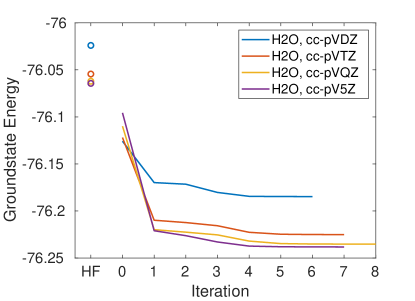
Figure 1: Convergence of the ground-state energy of H2O against iteration for $N=12$.

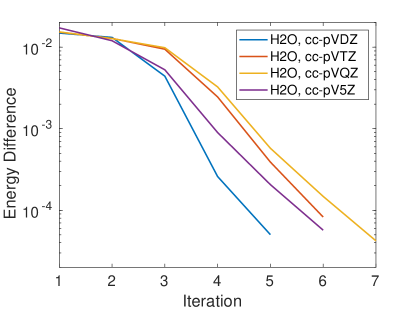
Figure 2: Difference of the ground-state energy of H2O against iteration for $N=12$.

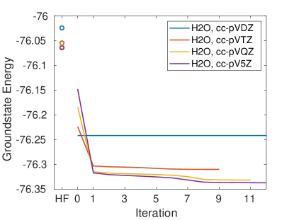
Figure 3: Convergence of the ground-state energy of H2O against iteration for $N=24$.

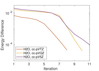
Figure 4: Difference of the ground-state energy of H2O against iteration for $N=24$.

Two different numbers of selected orbitals, $N=12$ and $N=24$, are tested for H2O molecules on a sequence of basis sets. Figure 1 and Figure 3 show the convergence behavior of OptOrbFCI against the iteration number for $N=12$ and $N=24$ respectively. The HF energies are also plotted in both figures with the $x$-axis label being “HF”. The energies associated with iteration $0$ is the FCI energies before applying projection method and the orbitals with smallest $N$ orbital energies are used as the selected orbitals. Figure 2 and Figure 4 further show the log scale of the energy difference against the iteration. Here the energy difference is defined as the difference between the FCI ground-state energy at current iteration and the converged FCI ground-state energy. In Figure 4, the curve associated with cc-pVDZ is removed since the ground-state energies stay constant throughout iterations. Table 2 lists all convergent FCI ground-state energies.

	$N=12$	$N=24$
Basis	GS energy	GS energy
cc-pVDZ	$-76.1846948$	$-76.2418601$
cc-pVTZ	$-76.2251082$	$-76.3102225$
cc-pVQZ	$-76.2352354$	$-76.3317350$
cc-pV5Z	$-76.2382165$	$-76.3372849$

Table 2: Ground-state energies for H2O with different number of selected orbitals under variant basis sets.

In both Figure 1 and Figure 3, we notice that all FCI ground-state energies are lower than HF energy under any these basis set. For the first FCI calculation with selected orbitals according to lowest orbital energies, i.e., iteration $0$, we observe that the smaller the basis set the lower the energy. This is likely due to the energy concentration of orbitals, which means that smaller basis set has better concentration of energies among occupied orbitals. As long as an optimized partial unitary matrix $U$ is applied, such an order no longer preserves starting from iteration $1$. In both cases, we also notice that the ordering of energies for different basis sets reveals after the first two iterations. Starting from then, larger basis sets consistently have lower ground-state energies than the smaller basis sets. The difference between the ground-state energies for different basis sets are much larger than the desired chemical accuracy. Further in Figure 2 and Figure 4, steady convergence is observed for all experiments and OptOrbFCI converges to chemical accuracy level within a few iterations. Larger $N$ leads to slightly more iterations in OptOrbFCI.

In addition to Figure 1 and Figure 3, Table 2 further illustrates ground-state energies for both $N=12$ and $N=24$. The difference between neighbour basis sets is decreasing as the basis set size increases. The decrease of energies from cc-pVQZ to cc-pV5Z for both $N$ are on the level of millihartree. Hence the basis limit is nearly achieved for H2O given $N=12$ and $N=24$.

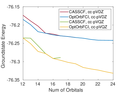
Figure 5: Convergence of the ground-state energy of H2O against varying $N$.

	OptOrbFCI		CASSCF
Orbs	GS energy	Iter	GS energy	Iter
12	$-76.1847$	6	$-76.1734$	7
13	$-76.1988$	8	$-76.1888$	7
14	$-76.2182$	8	$-76.2029$	7
15	$-76.2223$	7	$-76.2223$	7
16	$-76.2270$	10	$-76.2247$	7
17	$-76.2295$	6	$-76.2295$	7
18	$-76.2314$	6	$-76.2314$	6
19	$-76.2341$	3	$-76.2341$	5
20	$-76.2360$	3	$-76.2360$	4

Table 3: Comparison of OptOrbFCI and CASSCF ⁵⁷ for H2O under cc-pVDZ basis set. Gray row indicates significantly different ground-state energies for different methods. Orbs is the number of selected orbitals and Iter is the macro iteration number.

	OptOrbFCI		CASSCF
Orbs	GS energy	Iter	GS energy	Iter
12	$-76.2352$	8	$-76.2353$	19
13	$-76.2506$	7	$-76.2358$	6
14	$-76.2721$	9	$-76.2566$	6
15	$-76.2780$	5	$-76.2780$	6
16	$-76.2913$	15	$-76.2914$	19
17	$-76.2964$	18	$-76.2889$	8

Table 4: Comparison of OptOrbFCI and CASSCF ⁵⁷ for H2O under cc-pVQZ basis set.

The decrease of the energy as $N$ increases from $12$ to $24$ is still significant for all basis sets. Hence we further investigate the relationship between the ground-state energy and the number of selected orbitals, $N$. Figure 5 shows such a relationship under cc-pVDZ and cc-pVQZ basis sets. As shown in Figure 5, as we gradually increase the number of selected orbitals, the ground-state energy of cc-pVDZ basis set first decay rapidly for $N$ between $12$ to $15$, and then, for $N\geq 15$, the decay is much slower. The decay of the ground-state energy of cc-pVQZ basis set decreasing steadily for all $N$ tested here. Hence we expect the slow decay for cc-pVQZ basis set comes later than $N=24$. While, under limited computational budget, the ground-state energy for cc-pVQZ with $24$ selected orbitals is already much lower than that of cc-pVDZ with $24$ selected orbitals.

In addition to Figure 5, the comparison between OptOrbFCI and CASSCF is detailed in Table 3 and Table 4 for cc-pVDZ and cc-pVQZ basis sets respectively. In both tables, we highlight the rows with significantly different ground-state energies. In all cases, OptOrbFCI achieves lower energy. Since the original optimization problem (14) is non-convex, any method could be trapped in local minima especially for methods concerning local optimization. OptOrbFCI, using additive random perturbation to initializations in orbital optimization, in many cases avoids the local minima near the initial point. Hence we observe that OptOrbFCI in many cases achieves lower ground-state energy and in no case achieves higher ground-state energy. Here both methods use the same default initial one- and two-body integrals with respect to Hatree-Fock orbitals. When different initializations are considered, the results in Table 3 and Table 4 could be different. While OptOrbFCI is still expected to achieve energies lower or equal to that of CASSCF. If we further compare the macro iteration numbers, when both methods converge to the same ground-state energy, OptOrbFCI has less or equal number of macro iterations comparing to CASSCF. Even for those cases where lower ground-state energy is achieved by OptOrbFCI, the difference in macro iteration number is, in most cases, not significant. Hence we conclude that OptOrbFCI could achieve lower ground-state energy and reduce the macro iteration number.

4.2 C2 and N2

This section studies OptOrbFCI applied to C2 and N2 under their equilibrium geometry; i.e., the bond length for C2 is $1.24253$ Å ^{12, 14} and the bond length for N2 is $2.118$ $a_{0}$ ^{58, 14}.

The hyper parameters in OptOrbFCI are the same for C2 and N2. In CDFCI, the compression threshold is $5\times 10^{-6}$, the tolerance for convergence is $10^{-5}$, and the maximum number of iterations is $3\times 10^{7}$. In the projection method, the convergence tolerance is $10^{-7}$ and the maximum number of iterations is $10^{4}$. In OptOrbFCI, the convergence tolerance is $10^{-4}$ and the maximum number of iterations is $20$.

					Selected	Iteration	OptOrbFCI
Molecule	Basis	Electrons	Orbitals	HF energy	Orbitals	Number	GS energy
C2	cc-pVDZ	12	28	$-75.4168820$	28	-	$-75.7319604$
	cc-pVTZ	12	60	$-75.4014464$	28	6	$-75.7763001$
	cc-pVQZ	12	110	$-75.4057650$	28	10	$-75.7991578$
	cc-pV5Z	12	182	$-75.4065236$	28	12	$-75.8030425$

Table 5: Basis sets and numerical results for C2.

					Selected	Iteration	OptOrbFCI
Molecule	Basis	Electrons	Orbitals	HF energy	Orbitals	Number	GS energy
N2	cc-pVDZ	14	28	$-108.9493779$	28	-	$-109.2821727$
	cc-pVTZ	14	60	$-108.9775136$	28	7	$-109.3409252$
	cc-pVQZ	14	110	$-108.9849510$	28	7	$-109.3639435$
	cc-pV5Z	14	182	$-108.9866093$	28	13	$-109.3689430$

Table 6: Basis sets and numerical results for N2.

Table 5 and Table 6, for C2 and N2 respectively, show the properties of the dimers and our numerical results. Since OptOrbFCI selects the number of orbitals the same as that under the cc-pVDZ basis set, the ground-state energies of cc-pVDZ basis set are the FCI results and are used as reference for the rest results. Similar figures as in the case of H2O can also be plotted for C2 and N2. Since there is not much difference, we omit them from the paper.

Both Table 5 and Table 6 show similar properties and we discuss their numerical results together. First of all, we notice that any FCI ground-state energy is lower than all the HF energies, which shows that the improvement of the FCI calculation over the HF calculation is beyond the difference between basis sets. Since we fix the number of selected orbitals to the same as that under the cc-pVDZ basis set, the computational cost of the optimal orbital selection method for other basis sets remains the same order as the cost of FCI under the cc-pVDZ basis set. If only the ground-state energy is needed, then OptOrbFCI is roughly twice the iteration number more expensive then that of the FCI under cc-pVDZ. If both the ground-state energy and the RDMs are needed for downstream tasks, then the increasing factor is reduced to the iteration number, which is between $6$ and $13$. In these estimations, the computational cost of the projection method is ignored. This is the case for the cc-pVTZ and cc-pVQZ basis sets, while for the cc-pV5Z basis set, the computational cost of the projection method is still smaller than that of CDFCI part but of the same order. Now we provide a few numbers to support this. All the numerical results in this section are performed on a machine with Intel Xeon CPU E5-2687W v3 at 3.10 GHz and 500 GB memory. At least $6$ tasks are performed simultaneously. The memory for each problem is limited to 40 GB. Given $N$ selected orbitals, for all basis sets, each CDFCI part (FCI solver plus RDM calculations) costs varying from $10,000$ to $50,000$ seconds for C2, while the computational costs for the projection method parts are dramatically different for different basis sets. The projection method part costs nearly $200$ seconds, $3,000$ seconds, and $10,000$ seconds for the cc-pVTZ, cc-pVQZ, and cc-pV5Z basis sets respectively. The runtime for N2 has a similar ratio between the CDFCI part and the projection method.

Comparing the ground-state energies under different basis sets, we notice that the lower ground-state energy is achieved under the larger basis set. The improvement between consecutive basis sets, however, is gradually decreasing, close to exponential decay. For both C2 and N2, the improvement between the cc-pV5Z and cc-pVQZ basis sets is on the level of millihartree.

4.3 N2 Binding Curve

This section benchmarks the binding curve of N2 under the cc-pVQZ basis set with $N=28$, which is the number of orbitals under the cc-pVDZ basis set. The all-electron N2 binding curve is well-known to be a difficult problem due to the multireference property for geometry away from equilibrium. In Wang et al. ¹⁴, the binding curve on a very fine grid is produced under the cc-pVDZ basis set up to $10^{-3}$ mHa accuracy. Here we rebenchmark the binding curve under the cc-pVQZ basis set with $N=28$ selected orbitals with an accuracy up to $10^{-1}$ mHa. Since the number of orbitals remains the same, the computational cost of our optimal orbital selection is of the same order as a single CDFCI execution ¹⁴.

For the binding curve, exact same geometries as in Wang et al. ¹⁴ are produced. The compression threshold, for the CDFCI part, is $5\times 10^{-6}$, the tolerance for convergence is $10^{-5}$, and the maximum number of iterations is $3\times 10^{7}$. The convergence tolerance for the projection method is $10^{-7}$ and the maximum number of iterations is $10^{4}$. For OptOrbFCI, the convergence tolerance is $10^{-4}$ and the maximum number of iterations is $20$.

Figure 6: Binding curves for N2. The blue curve is cited from CDFCI ¹⁴. For each bond length, OptOrbFCI selects $28$ orbitals under cc-pVQZ basis set.

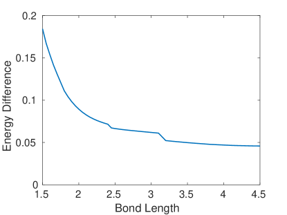
Figure 7: Difference of binding curves for N2 using FCI under cc-PVDZ basis set and OptOrbFCI under cc-pVQZ basis set with $N=28$.

				GS energy	GS energy	Dissociation
Method	Basis	Electrons	Orbitals	2.118 $a_{0}$	4.5 $a_{0}$	energy
FCI	cc-pVDZ	14	28	$-109.2821727$	$-108.9659102$	$0.3162625$
	cc-pVQZ	14	110	$-109.4590412$	$-109.1059938$	$0.3530474$
OptOrbFCI	cc-pVQZ	14	28	$-109.3639435$	$-109.0117220$	$0.3522214$

Table 7: Dissociation energy for N2. FCI results are calculated through CDFCI.

Figure 6 illustrates the binding curves of N2 calculated from CDFCI under cc-pVDZ basis set ¹⁴ and from OptOrbFCI under cc-pVQZ basis set with $N=28$. From the figure, in all geometries, OptOrbFCI provides lower variational ground-state energies, while the overall shapes for two curves remain similar. Figure 7 further shows the energy difference of two binding curves, i.e., the ground-state energy of CDFCI minus that of OptOrbFCI. We observe that the decrease is more dramatic when two atoms are closer. There are two non-smooth points in the energy difference around $2.45a_{0}$ and $3.2a_{0}$. Numerically, we also find that the computation is more difficult around these two bond lengths, i.e., the number of iterations increases. Further investigation is needed around these two points.

Comparing to the single ground-state energy, the energy gap is of more chemical relevance. Here, we also include the dissociation energies for $\ch{N2}$ under three settings. The dissociation energy is defined as the difference of ground-state energies at equilibrium geometry (2.118 $a_{0}$) and at well separated geometry (4.5 $a_{0}$). Three settings are FCI under cc-pVDZ, FCI under cc-pVQZ, and OptOrbFCI under cc-pVQZ with $N=28$. Numerical results are listed in Table 7. Using the dissociation energy of FCI under cc-pVQZ as a reference solution, we notice that the dissociation energy of OptOrbFCI is more accurate than that of FCI under cc-pVDZ. The error for FCI under cc-pVDZ is about $4\times 10^{-2}$ Ha whereas the error for OptOrbFCI is about $10^{-3}$, which is on the level of chemical accuracy. Hence we conclude that OptOrbFCI, in addition to provide lower ground-state energies, provides more accurate dissociation energy.

5 Conclusion and Discussion

We consider the question in this paper for full configuration interaction (FCI) pursuing the basis set limit under a computational budget. We propose a coupled optimization problem (14) as a solution to the question, which is also the formula for CASSCF. The coupling therein between the ground-state wave function $\ket{\Phi}$ and the partial unitary matrix $U$ is complicated. Due to the complication, the optimization problem (14) is then split into two subproblems, (16) and (18), where the former is a standard FCI problem under compressed orbitals and the latter is an optimization of a 4 th order polynomial of $U$ with orthonormality constraint. An overall alternating iterative algorithm is proposed to address the optimization problem (14) with the first subproblem (16) solved by a wave function based FCI solver, namely CDFCI ¹⁴ and the second subproblem (18) solved by a projection method ⁴⁶. The overall method above is referred as OptOrbFCI. The method in general is efficient and stable. OptOrbFCI usually converges in 5 to 15 iterations to achieve up to $10^{-1}$ mHa accuracy. The computational cost, hence, is bounded by that of a few executions of the FCI solver on the selected orbital sets.

Numerically, we apply OptOrbFCI to the water molecule, carbon dimer, and nitrogen dimer under variant basis sets. Under the number of orbitals using the cc-pVDZ basis set, we pursue the FCI calculation under cc-pVTZ, cc-pVQZ, and cc-pV5Z basis sets. In all cases, we obtain ground-state energies lower than that under cc-pVDZ, where the decrease is beyond chemical accuracy. In the comparison against the conventional CASSCF method ⁵⁷, OptOrbFCI could achieve lower ground-state energy and reduce the macro iteration number. N2 binding curve is rebenchmarked using OptOrbFCI under the cc-pVQZ basis set with $28$ selected orbitals. And the dissociation energy in this case is more accurate than that obtained by the FCI solver under the cc-pVDZ basis set. Hence we conclude that OptOrbFCI coupling with existing FCI solvers is able to pursue the basis set limit under a computational budget.

There are a list of immediate future works of OptOrbFCI. In the current implementation, the orbital symmetry in the given large orbital set is totally ignored; so is the frozen core setting. Under the given large orbital set with orbital symmetry, both the one-body and two-body integrals are of sparse structure. As we ignored the symmetry and frozen core setting, the one-body and two-body integrals of the rotated orbitals are then dense tensors. The downstream FCI problem becomes more expensive. Hence one future work is to implement the rotation under an orbital symmetry constraint and frozen core setting to reduce the cost of FCI solvers. When orbital symmetries are preserved, the corresponding ground-state energy will be lower bounded by that of our current algorithm. Further investigation is needed on the trade-off between the accuracy and the computational cost. A parallelization of the projection method becomes important when the basis set gets large, since the computational bottleneck for the projection method lies in the 4-way tensor contraction, which can be realized as a dense matrix-matrix multiplication. Efficient both distributed-memory and shared-memory parallelizations are manageable. Highly efficient GPU acceleration can also be expected. Besides implementation, further investigation of the convergence property is desired. And extension to low-lying excited states calculation is also a promising future work to be explored. When both ground-state and low-lying excited states are considered under the OptOrbFCI framework with a modified objective function, we expect that the optimal rotation matrix would balance the error among states under consideration and hence potentially provide more accurate approximation to excitation energies than our current algorithm.

The authors thank Zhe Wang for helpful discussions. The authors also thank Jonathon Misiewicz and Qiming Sun for constructive suggestions on the comparison with CASSCF. The work is supported in part by the US National Science Foundation under awards DMS-1454939 and DMS-2012286, and by the US Department of Energy via grant DE-SC0019449.

Appendix A Equivalence between (10) and (14)

This section provides detailed derivations for the equivalence between (10) and (14). The key step is to show that (13) holds for any wave function $\ket{\Phi}$ in $\mathcal{D}[(\psi_{1},\dots,\psi_{M})U]=\mathcal{D}[(\phi_{1},\dots,\phi_{N})]$. Since the operators are linear operators and the space is a linear space, it is sufficient to show that (13) holds for all bases in $\mathcal{D}[(\phi_{1},\dots,\phi_{N})]$, i.e., all Slater determinants. Any Slater determinant $\ket{D_{i}}$ in $\mathcal{D}[(\phi_{1},\dots,\phi_{N})]$ can be written as,

$$\ket{D_{i}}=\hat{\boldsymbol{d}}_{i_{1}}^{\dagger}\cdots\hat{\boldsymbol{d}}_{i_{n_{\text{e}}}}^{\dagger}\ket{0}$$ (35)

where $i_{1},\dots,i_{n_{\text{e}}}$ are the index of $n_{\text{e}}$ occupied orbitals and $\ket{0}$ denotes vacuum state. Now we evaluate the difference of acting $\hat{\boldsymbol{c}}_{q}$ and $\tilde{\boldsymbol{c}}_{q}$ on such a Slater determinant. Using the anticommutation relation (11) and (12), the difference can be simplified as,

$$\begin{split}&\big{(}\hat{\boldsymbol{c}}_{q}-\tilde{\boldsymbol{c}}_{q}\big{)}\ket{D_{i}}\\ =&\big{(}\hat{\boldsymbol{c}}_{q}-\tilde{\boldsymbol{c}}_{q}\big{)}\hat{\boldsymbol{d}}_{i_{1}}^{\dagger}\cdots\hat{\boldsymbol{d}}_{i_{n_{\text{e}}}}^{\dagger}\ket{0}\\ =&\Big{(}\anticommutator{\hat{\boldsymbol{c}}_{q}}{\hat{\boldsymbol{d}}_{i_{1}}^{\dagger}}-\anticommutator{\tilde{\boldsymbol{c}}_{q}}{\hat{\boldsymbol{d}}_{i_{1}}^{\dagger}}\Big{)}\hat{\boldsymbol{d}}_{i_{2}}^{\dagger}\cdots\hat{\boldsymbol{d}}_{i_{n_{\text{e}}}}^{\dagger}\ket{0}\\ &-\hat{\boldsymbol{d}}_{i_{1}}^{\dagger}\big{(}\hat{\boldsymbol{c}}_{q}-\tilde{\boldsymbol{c}}_{q}\big{)}\hat{\boldsymbol{d}}_{i_{2}}^{\dagger}\cdots\hat{\boldsymbol{d}}_{i_{n_{\text{e}}}}^{\dagger}\ket{0}\\ =&-\hat{\boldsymbol{d}}_{i_{1}}^{\dagger}\big{(}\hat{\boldsymbol{c}}_{q}-\tilde{\boldsymbol{c}}_{q}\big{)}\hat{\boldsymbol{d}}_{i_{2}}^{\dagger}\cdots\hat{\boldsymbol{d}}_{i_{n_{\text{e}}}}^{\dagger}\ket{0}\\ =&(-1)^{k}\hat{\boldsymbol{d}}_{i_{1}}^{\dagger}\cdots\hat{\boldsymbol{d}}_{i_{k}}^{\dagger}\big{(}\hat{\boldsymbol{c}}_{q}-\tilde{\boldsymbol{c}}_{q}\big{)}\hat{\boldsymbol{d}}_{i_{k+1}}^{\dagger}\cdots\hat{\boldsymbol{d}}_{i_{n_{\text{e}}}}^{\dagger}\ket{0}\\ =&(-1)^{n_{\text{e}}}\hat{\boldsymbol{d}}_{i_{1}}^{\dagger}\cdots\hat{\boldsymbol{d}}_{i_{n_{\text{e}}}}^{\dagger}\big{(}\hat{\boldsymbol{c}}_{q}-\tilde{\boldsymbol{c}}_{q}\big{)}\ket{0}\\ =&0,\end{split}$$ (36)

where the last equality holds since the annihilation operators acting on the vacuum state vanish. Since any wave function $\ket{\Phi}\in\mathcal{D}[(\phi_{1},\dots,\phi_{N})]$ can be expressed as a linear combination of Slater determinants, i.e., $\ket{\Phi}=\sum_{i}x_{i}\ket{D_{i}}$, where $x_{i}$ are coefficients, acting the difference of $\hat{\boldsymbol{c}}_{q}$ and $\tilde{\boldsymbol{c}}_{q}$ on it leads to,

$$\big{(}\hat{\boldsymbol{c}}_{q}-\tilde{\boldsymbol{c}}_{q}\big{)}\ket{\Phi}=\sum_{i}x_{i}\big{(}\hat{\boldsymbol{c}}_{q}-\tilde{\boldsymbol{c}}_{q}\big{)}\ket{D_{i}}=0.$$ (37)

Hence we showed that (13) holds for all $\ket{\Phi}\in\mathcal{D}[(\phi_{1},\dots,\phi_{N})]$. The conjugate of (13) gives,

$$\bra{\Phi}\hat{\boldsymbol{c}}_{p}^{\dagger}=\bra{\Phi}\tilde{\boldsymbol{c}}_{p}^{\dagger}.$$ (38)

The one-body part in the objective function in (10) then admits,

$$\begin{split}&\expectationvalue{\sum_{p,q=1}^{M}h_{pq}\hat{\boldsymbol{c}}_{p}^{\dagger}\hat{\boldsymbol{c}}_{q}}{\Phi}\\ =&\sum_{p,q=1}^{M}h_{pq}\expectationvalue{\tilde{\boldsymbol{c}}_{p}^{\dagger}\tilde{\boldsymbol{c}}_{q}}{\Phi}\\ =&\sum_{p,q=1}^{M}h_{pq}\sum_{p^{\prime},q^{\prime}=1}^{N}\expectationvalue{\hat{\boldsymbol{d}}_{p^{\prime}}^{\dagger}\hat{\boldsymbol{d}}_{q^{\prime}}}{\Phi}U_{pp^{\prime}}U_{qq^{\prime}}\\ =&\expectationvalue{\sum_{p^{\prime},q^{\prime}=1}^{N}\tilde{h}_{p^{\prime}q^{\prime}}\hat{\boldsymbol{d}}_{p^{\prime}}^{\dagger}\hat{\boldsymbol{d}}_{q^{\prime}}}{\Phi},\\ \end{split}$$ (39)

where $\tilde{h}_{p^{\prime}q^{\prime}}$ is defined as (7). The one-body part in the objective function in (10), hence, is equivalent to that in (14).

In order to show the equivalence of the two-body part in both objective functions, we need two more anticommutation relations. The anticommutation relation between $\hat{\boldsymbol{c}}_{s}$ and $\tilde{\boldsymbol{c}}_{r}$ satisfies,

$$\begin{split}\anticommutator{\hat{\boldsymbol{c}}_{s}}{\tilde{\boldsymbol{c}}_{r}}=&\anticommutator{\hat{\boldsymbol{c}}_{s}}{\sum_{r^{\prime}=1}^{N}\hat{\boldsymbol{d}}_{r^{\prime}}U_{rr^{\prime}}}\\ =&\sum_{r^{\prime}=1}^{N}\sum_{r^{\prime\prime}=1}^{M}\anticommutator{\hat{\boldsymbol{c}}_{s}}{\hat{\boldsymbol{c}}_{r^{\prime\prime}}}U_{rr^{\prime}}U_{r^{\prime\prime}r^{\prime}}\\ =&0.\end{split}$$ (40)

Similarly, we also have the anticommutation relation between $\tilde{\boldsymbol{c}}_{p}^{\dagger}$ and $\hat{\boldsymbol{c}}_{q}^{\dagger}$,

$$\anticommutator{\tilde{\boldsymbol{c}}_{p}^{\dagger}}{\hat{\boldsymbol{c}}_{q}^{\dagger}}=0.$$ (41)

The anti-commutation relations within $\tilde{\boldsymbol{c}}$s can also be derived in an analog way. The two-body part in the objective function in (10) then admits,

$$\begin{split}&\expectationvalue{\sum_{p,q,r,s=1}^{M}v_{pqrs}\hat{\boldsymbol{c}}_{p}^{\dagger}\hat{\boldsymbol{c}}_{q}^{\dagger}\hat{\boldsymbol{c}}_{s}\hat{\boldsymbol{c}}_{r}}{\Phi}\\ =&\sum_{p,q,r,s=1}^{M}v_{pqrs}\expectationvalue{\tilde{\boldsymbol{c}}_{p}^{\dagger}\hat{\boldsymbol{c}}_{q}^{\dagger}\hat{\boldsymbol{c}}_{s}\tilde{\boldsymbol{c}}_{r}}{\Phi}\\ =&\sum_{p,q,r,s=1}^{M}v_{pqrs}\expectationvalue{\hat{\boldsymbol{c}}_{q}^{\dagger}\tilde{\boldsymbol{c}}_{p}^{\dagger}\tilde{\boldsymbol{c}}_{r}\hat{\boldsymbol{c}}_{s}}{\Phi}\\ =&\sum_{p,q,r,s=1}^{M}v_{pqrs}\expectationvalue{\tilde{\boldsymbol{c}}_{p}^{\dagger}\tilde{\boldsymbol{c}}_{q}^{\dagger}\tilde{\boldsymbol{c}}_{s}\tilde{\boldsymbol{c}}_{r}}{\Phi}\\ =&\sum_{p^{\prime},q^{\prime},r^{\prime},s^{\prime}=1}^{N}\sum_{p,q,r,s=1}^{M}v_{pqrs}U_{pp^{\prime}}U_{qq^{\prime}}U_{rr^{\prime}}U_{ss^{\prime}}\cdot\\ &\cdot\expectationvalue{\hat{\boldsymbol{d}}_{p^{\prime}}^{\dagger}\hat{\boldsymbol{d}}_{q^{\prime}}^{\dagger}\hat{\boldsymbol{d}}_{s^{\prime}}\hat{\boldsymbol{d}}_{r^{\prime}}}{\Phi}\\ =&\expectationvalue{\sum_{p^{\prime},q^{\prime},r^{\prime},s^{\prime}=1}^{M}\tilde{v}_{p^{\prime}q^{\prime}r^{\prime}s^{\prime}}\hat{\boldsymbol{d}}_{p^{\prime}}^{\dagger}\hat{\boldsymbol{d}}_{q^{\prime}}^{\dagger}\hat{\boldsymbol{d}}_{s^{\prime}}\hat{\boldsymbol{d}}_{r^{\prime}}}{\Phi},\\ \end{split}$$ (42)

where the second equality applies the anticommutation relations in (40) and (41), the third equality applies the anticommutation relations within $\tilde{\boldsymbol{c}}$s, and $\tilde{v}_{p^{\prime}q^{\prime}r^{\prime}s^{\prime}}$ is defined as (8). The two-body part in the objective function in (10), hence, is equivalent to that in (14).

Combining (39) and (42), we conclude that the objective functions in (10) and (14) are equivalent given the wave function $\ket{\Phi}\in\mathcal{D}[(\phi_{1},\dots,\phi_{N})]$.

Appendix B N2 Binding Curve

The N2 binding curve is plotted in Figure 6 and the detailed energies are given in Table 8 and Table 9. Table 8 provides the ground-state energies for N2 with bond length smaller than that at equilibrium geometry, whereas Table 9 provides the ground-state energies with bond length greater than that at equilibrium geometry. In both tables, we apply OptOrbFCI to compute the ground-state energies of N2 under the cc-pVQZ basis set with 28 selected orbitals. The same list of bond lengths as that in Wang et al. ¹⁴ is adopted here. The ground-state energies of FCI under the cc-pVDZ basis set are cited from Wang et al. ¹⁴.

Bond	FCI	OptOrb
Length ($a_{0}$)	cc-pVDZ (Ha)	cc-pVQZ(28) (Ha)
1.500	$-108.6300476$	$-108.8144031$
1.550	$-108.7719968$	$-108.9391824$
1.600	$-108.8888460$	$-109.0429050$
1.650	$-108.9843136$	$-109.1260152$
1.700	$-109.0615754$	$-109.1926550$
1.750	$-109.1233484$	$-109.2443696$
1.800	$-109.1719641$	$-109.2830113$
1.850	$-109.2094264$	$-109.3137005$
1.900	$-109.2374578$	$-109.3359754$
1.950	$-109.2575411$	$-109.3511562$
2.000	$-109.2709530$	$-109.3603603$
2.050	$-109.2787896$	$-109.3645818$
2.100	$-109.2819938$	$-109.3647561$
2.118	$-109.2821727$	$-109.3639435$

Table 8: Ground state energies for N2 with bond lengths smaller than $2.118a_{0}$.

Bond	FCI	OptOrb
Length ($a_{0}$)	cc-pVDZ (Ha)	cc-pVQZ(28) (Ha)
2.118	$-109.2821727$	$-109.3639435$
2.150	$-109.2813737$	$-109.3614955$
2.200	$-109.2776211$	$-109.3555534$
2.250	$-109.2713283$	$-109.3473397$
2.300	$-109.2630013$	$-109.3373910$
2.350	$-109.2530718$	$-109.3259793$
2.400	$-109.2419079$	$-109.3135325$
2.450	$-109.2298228$	$-109.2970156$
2.500	$-109.2170830$	$-109.2835331$
2.600	$-109.1905077$	$-109.2557994$
2.700	$-109.1635998$	$-109.2279395$
2.800	$-109.1373583$	$-109.2008712$
2.900	$-109.1124729$	$-109.1751472$
3.000	$-109.0894053$	$-109.1512795$
3.100	$-109.0684502$	$-109.1295149$
3.200	$-109.0497787$	$-109.1020069$
3.300	$-109.0334619$	$-109.0848174$
3.400	$-109.0194835$	$-109.0700669$
3.500	$-109.0077466$	$-109.0575569$
3.600	$-108.9980829$	$-109.0471986$
3.700	$-108.9902691$	$-109.0387653$
3.800	$-108.9840499$	$-109.0319008$
3.900	$-108.9791625$	$-109.0265483$
4.000	$-108.9753572$	$-109.0223481$
4.100	$-108.9724102$	$-109.0189859$
4.200	$-108.9701316$	$-109.0164481$
4.300	$-108.9683664$	$-109.0144948$
4.400	$-108.9669909$	$-109.0129196$
4.500	$-108.9659102$	$-109.0117220$

Table 9: Ground state energies for N2 with bond lengths larger than $2.118a_{0}$.

References

- Chan and Sharma 2011 Chan, G. K.-L.; Sharma, S. The density matrix renormalization group in quantum chemistry. Annu. Rev. Phys. Chem. 2011, 62, 465–481
- Olivares-Amaya \latinet al. 2015 Olivares-Amaya, R.; Hu, W.; Nakatani, N.; Sharma, S.; Yang, J.; Chan, G. K.-L. The ab-initio density matrix renormalization group in practice. J. Chem. Phys. 2015, 142, 034102
- Booth \latinet al. 2009 Booth, G. H.; Thom, A. J. W.; Alavi, A. Fermion Monte Carlo without fixed nodes: A game of life, death, and annihilation in Slater determinant space. J. Chem. Phys. 2009, 131, 054106
- Booth \latinet al. 2012 Booth, G. H.; Grüneis, A.; Kresse, G.; Alavi, A. Towards an exact description of electronic wavefunctions in real solids. Nature 2012, 493, 365–370
- Cleland \latinet al. 2010 Cleland, D.; Booth, G. H.; Alavi, A. Communications: Survival of the fittest: Accelerating convergence in full configuration-interaction quantum Monte Carlo. J. Chem. Phys. 2010, 132, 041103
- Petruzielo \latinet al. 2012 Petruzielo, F. R.; Holmes, A. A.; Changlani, H. J.; Nightingale, M. P.; Umrigar, C. J. Semistochastic projector Monte Carlo method. Phys. Rev. Lett. 2012, 109, 230201
- Lu and Wang 2020 Lu, J.; Wang, Z. The full configuration interaction quantum Monte Carlo method in the lens of inexact power iteration. SIAM J. Sci. Comput. 2020, 42, B1–B29
- Huron \latinet al. 1973 Huron, B.; Malrieu, J. P.; Rancurel, P. Iterative perturbation calculations of ground and excited state energies from multiconfigurational zeroth-order wavefunctions. J. Chem. Phys. 1973, 58, 5745–5759
- Schriber and Evangelista 2016 Schriber, J. B.; Evangelista, F. A. Communication: An adaptive configuration interaction approach for strongly correlated electrons with tunable accuracy. J. Chem. Phys. 2016, 144, 161106
- Tubman \latinet al. 2016 Tubman, N. M.; Lee, J.; Takeshita, T. Y.; Head-Gordon, M.; Whaley, K. B. A deterministic alternative to the full configuration interaction quantum Monte Carlo method. J. Chem. Phys. 2016, 145, 044112
- Tubman \latinet al. 2018 Tubman, N. M.; Freeman, C. D.; Levine, D. S.; Hait, D.; Head-Gordon, M.; Whaley, K. B. Modern approaches to exact diagonalization and selected configuration interaction with the adaptive sampling CI method. 2018; http://arxiv.org/abs/1807.00821
- Holmes \latinet al. 2016 Holmes, A. A.; Tubman, N. M.; Umrigar, C. J. Heat-bath configuration interaction: An efficient selected configuration interaction algorithm inspired by heat-bath sampling. J. Chem. Theory Comput. 2016, 12, 3674–3680
- Sharma \latinet al. 2017 Sharma, S.; Holmes, A. A.; Jeanmairet, G.; Alavi, A.; Umrigar, C. J. Semistochastic heat-bath configuration interaction method: Selected configuration interaction with semistochastic perturbation theory. J. Chem. Theory Comput. 2017, 13, 1595–1604
- Wang \latinet al. 2019 Wang, Z.; Li, Y.; Lu, J. Coordinate descent full configuration interaction. J. Chem. Theory Comput. 2019, 15, 3558–3569
- Greene \latinet al. 2019 Greene, S. M.; Webber, R. J.; Weare, J.; Berkelbach, T. C. Beyond walkers in stochastic quantum chemistry: Reducing error using fast randomized iteration. 2019; http://arxiv.org/abs/1905.00995
- Lim and Weare 2017 Lim, L.-H.; Weare, J. Fast randomized iteration: Diffusion Monte Carlo through the lens of numerical linear algebra. SIAM Rev. 2017, 59, 547–587
- Li \latinet al. 2019 Li, Y.; Lu, J.; Wang, Z. Coordinatewise descent methods for leading eigenvalue problem. SIAM J. Sci. Comput. 2019, 41, A2681–A2716
- Hernandez \latinet al. 2019 Hernandez, T. M.; Van Beeumen, R.; Caprio, M. A.; Yang, C. A greedy algorithm for computing eigenvalues of a symmetric matrix. 2019; http://arxiv.org/abs/1911.10041
- Gao \latinet al. 2020 Gao, W.; Li, Y.; Lu, B. Triangularized orthogonalization-free method for solving extreme eigenvalue problems. 2020; http://arxiv.org/abs/2005.12161
- Bytautas \latinet al. 2003 Bytautas, L.; Ivanic, J.; Ruedenberg, K. Split-localized orbitals can yield stronger configuration interaction convergence than natural orbitals. J. Chem. Phys. 2003, 119, 8217–8224
- Zhang and Kollar 2014 Zhang, J. M.; Kollar, M. Optimal multiconfiguration approximation of an -fermion wave function. Phys. Rev. A - At. Mol. Opt. Phys. 2014, 89, 012504
- Giesbertz 2014 Giesbertz, K. J. H. Are natural orbitals useful for generating an efficient expansion of the wave function? Chem. Phys. Lett. 2014, 591, 220–226
- Alcoba \latinet al. 2016 Alcoba, D. R.; Torre, A.; Lain, L.; Massaccesi, G. E.; Oña, O. B.; Ayers, P. W.; Van Raemdonck, M.; Bultinck, P.; Van Neck, D. Performance of Shannon-entropy compacted -electron wave functions for configuration interaction methods. Theor. Chem. Acc. 2016, 135, 153
- Kivlichan \latinet al. 2018 Kivlichan, I. D.; McClean, J. R.; Wiebe, N.; Gidney, C.; Aspuru-Guzik, A.; Chan, G. K.-L.; Babbush, R. Quantum simulation of electronic structure with linear depth and connectivity. Phys. Rev. Lett. 2018, 120, 110501
- Babbush \latinet al. 2019 Babbush, R.; Berry, D. W.; McClean, J. R.; Neven, H. Quantum simulation of chemistry with sublinear scaling in basis size. npj Quantum Inf. 2019, 5, 1–7
- Siegbahn \latinet al. 1980 Siegbahn, P. E.; Heiberg, A.; Roos, B.; Levy, B. A comparison of the super-Cl and the Newton-Raphson scheme in the complete active space SCF method. Phys. Scr. 1980, 21, 323–237
- Roos \latinet al. 1980 Roos, B. O.; Taylor, P. R.; Sigbahn, P. E. A complete active space SCF method (CASSCF) using a density matrix formulated super-CI approach. Chem. Phys. 1980, 48, 157–173
- Siegbahn \latinet al. 1981 Siegbahn, P. E.; Almlöf, J.; Heiberg, A.; Roos, B. O. The complete active space SCF (CASSCF) method in a Newton-Raphson formulation with application to the HNO molecule. J. Chem. Phys. 1981, 74, 2384–2396
- Knowles and Werner 1985 Knowles, P. J.; Werner, H. J. An efficient second-order MC SCF method for long configuration expansions. Chem. Phys. Lett. 1985, 115, 259–267
- Zgid and Nooijen 2008 Zgid, D.; Nooijen, M. The density matrix renormalization group self-consistent field method: Orbital optimization with the density matrix renormalization group method in the active space. The Journal of Chemical Physics 2008, 128, 144116
- Ghosh \latinet al. 2008 Ghosh, D.; Hachmann, J.; Yanai, T.; Chan, G. K.-L. Orbital optimization in the density matrix renormalization group, with applications to polyenes and -carotene. The Journal of Chemical Physics 2008, 128, 144117
- Yanai \latinet al. 2009 Yanai, T.; Kurashige, Y.; Ghosh, D.; Chan, G. K.-L. Accelerating convergence in iterative solution for large-scale complete active space self-consistent-field calculations. Int. J. Quantum Chem. 2009, 109, 2178–2190
- Olsen 2011 Olsen, J. The CASSCF method: A perspective and commentary. Int. J. Quantum Chem. 2011, 111, 3267–3272
- Wouters \latinet al. 2014 Wouters, S.; Bogaerts, T.; Van Der Voort, P.; Van Speybroeck, V.; Van Neck, D. Communication: DMRG-SCF study of the singlet, triplet, and quintet states of oxo-Mn(Salen). Journal of Chemical Physics 2014, 140, 241103
- Li Manni \latinet al. 2016 Li Manni, G.; Smart, S. D.; Alavi, A. Combining the complete active space self-consistent field method and the full configuration interaction quantum Monte Carlo within a super-CI framework, with application to challenging metal-porphyrins. J. Chem. Theory Comput. 2016, 12, 1245–1258
- Freitag \latinet al. 2017 Freitag, L.; Knecht, S.; Angeli, C.; Reiher, M. Multireference perturbation theory with Cholesky decomposition for the density matrix renormalization group. Journal of Chemical Theory and Computation 2017, 13, 451–459, PMID: 28094988
- Ma \latinet al. 2017 Ma, Y.; Knecht, S.; Keller, S.; Reiher, M. Second-order self-consistent-field density-matrix renormalization group. J. Chem. Theory Comput. 2017, 13, 2533–2549
- Smith \latinet al. 2017 Smith, J. E.; Mussard, B.; Holmes, A. A.; Sharma, S. Cheap and near exact CASSCF with large active spaces. J. Chem. Theory Comput. 2017, 13, 5468–5478
- Sun \latinet al. 2017 Sun, Q.; Yang, J.; Chan, G. K. L. A general second order complete active space self-consistent-field solver for large-scale systems. Chem. Phys. Lett. 2017, 683, 291–299
- Freitag \latinet al. 2019 Freitag, L.; Ma, Y.; Baiardi, A.; Knecht, S.; Reiher, M. Approximate analytical gradients and nonadiabatic couplings for the state-average density matrix renormalization group self-consistent-field method. J. Chem. Theory Comput. 2019, 15, 6724–6737
- Kreplin \latinet al. 2019 Kreplin, D. A.; Knowles, P. J.; Werner, H. J. Second-order MCSCF optimization revisited. I. Improved algorithms for fast and robust second-order CASSCF convergence. J. Chem. Phys. 2019, 150, 194106
- Levine \latinet al. 2020 Levine, D. S.; Hait, D.; Tubman, N. M.; Lehtola, S.; Whaley, K. B.; Head-Gordon, M. CASSCF with extremely large active spaces using the adaptive sampling configuration interaction method. J. Chem. Theory Comput. 2020,
- Ruedenberg \latinet al. 1979 Ruedenberg, K.; Cheung, L. M.; Elbert, S. T. MCSCF optimization through combined use of natural orbitals and the Brillouin-Levy-Berthier theorem. Int. J. Quantum Chem. 1979, 16, 1069–1101
- Wen and Yin 2013 Wen, Z.; Yin, W. A feasible method for optimization with orthogonality constraints. Math. Program. 2013, 142, 397–434
- Gao \latinet al. 2019 Gao, B.; Liu, X.; Yuan, Y.-x. Parallelizable algorithms for optimization problems with orthogonality constraints. SIAM J. Sci. Comput. 2019, 41, A1949–A1983
- Gao \latinet al. 2018 Gao, B.; Liu, X.; Chen, X.; Yuan, Y. X. A new first-order algorithmic framework for optimization problems with orthogonality constraints. SIAM J. Optim. 2018, 28, 302–332
- Zhang \latinet al. 2014 Zhang, X.; Zhu, J.; Wen, Z.; Zhou, A. Gradient type optimization methods for electronic structure calculations. SIAM J. Sci. Comput. 2014, 36, C265–C289
- Huang \latinet al. 2015 Huang, W.; Gallivan, K. A.; Absil, P.-A. A Broyden class of quasi-Newton methods for Riemannian optimization. SIAM J. Optim. 2015, 25, 1660–1685
- Li Manni and Alavi 2018 Li Manni, G.; Alavi, A. Understanding the mechanism stabilizing intermediate spin states in Fe(II)-porphyrin. J. Phys. Chem. A 2018, 122, 4935–4947
- Deng and Yin 2016 Deng, W.; Yin, W. On the global and linear convergence of the generalized alternating direction method of multipliers. J. Sci. Comput. 2016, 66, 889–916
- Nesterov 2012 Nesterov, Y. Efficiency of coordinate descent methods on huge-scale optimization problems. SIAM J. Optim. 2012, 22, 341–362
- Wright 2015 Wright, S. J. Coordinate descent algorithms. Math. Program. 2015, 151, 3–34
- Shi \latinet al. 2016 Shi, H.-J. M.; Tu, S.; Xu, Y.; Yin, W. A primer on coordinate descent algorithms. 2016; http://arxiv.org/abs/1610.00040
- Banerjee and Grein 1976 Banerjee, A. S.; Grein, F. Convergence behavior of some multiconfiguration methods. Int. J. Quantum Chem. 1976, 10, 123–134
- Parrish \latinet al. 2017 Parrish, R. M.; Burns, L. A.; Smith, D. G. A.; Simmonett, A. C.; DePrince, A. E.; Hohenstein, E. G.; Bozkaya, U.; Sokolov, A. Y.; Di Remigio, R.; Richard, R. M.; Gonthier, J. F.; James, A. M.; McAlexander, H. R.; Kumar, A.; Saitow, M.; Wang, X.; Pritchard, B. P.; Verma, P.; Schaefer, H. F.; Patkowski, K.; King, R. A.; Valeev, E. F.; Evangelista, F. A.; Turney, J. M.; Crawford, T. D.; Sherrill, C. D. Psi4 1.1: An open-source electronic structure program emphasizing automation, advanced libraries, and interoperability. Journal of Chemical Theory and Computation 2017, 13, 3185–3197
- Wang \latinet al. 2020 Wang, Z.; Li, Y.; Lu, J. CDFCI. 2020; https://github.com/quan-tum/CDFCI
- Sun \latinet al. 2017 Sun, Q.; Berkelbach, T. C.; Blunt, N. S.; Booth, G. H.; Guo, S.; Li, Z.; Liu, J.; McClain, J. D.; Sayfutyarova, E. R.; Sharma, S.; Wouters, S.; Chan, G. K. PySCF: the Python-based simulations of chemistry framework. 2017; \urlhttps://onlinelibrary.wiley.com/doi/abs/10.1002/wcms.1340
- Chan \latinet al. 2004 Chan, G. K. L.; Kállay, M.; Gauss, J. State-of-the-art density matrix renormalization group and coupled cluster theory studies of the nitrogen binding curve. J. Chem. Phys. 2004, 121, 6110–6116