Possible Production of Solar Spicules by Microfilament Eruptions

Abstract

We examine Big Bear Solar Observatory (BBSO) Goode Solar Telescope (GST) high-spatial resolution ($0^{\prime\prime}.06$), high-cadence (3.45 s), H$\alpha$-0.8-Å images of central-disk solar spicules, using data of Samanta et al. (2019). We compare with coronal-jet chromospheric-component observations of Sterling et al. (2010a). Morphologically, bursts of spicules, referred to as “enhanced spicular activities” by Samanta et al. (2019), appear as scaled-down versions of the jet’s chromospheric component. Both the jet and the enhanced spicular activities appear as chromospheric-material strands, undergoing twisting-type motions of $\sim$20—50 km s^-1 in the jet and $\sim$20—30 km s^-1 in the enhanced spicular activities. Presumably, the jet resulted from a minifilament-carrying magnetic eruption. For two enhanced spicular activities that we examine in detail, we find tentative candidates for corresponding erupting microfilaments, but not expected corresponding base brightenings. Nonetheless, the enhanced-spicular-activities’ interacting mixed-polarity base fields, frequent-apparent-twisting motions, and morphological similarities to the coronal jet’s chromospheric-temperature component, suggest that erupting microfilaments might drive the enhanced spicular activities but be hard to detect, perhaps due to H$\alpha$ opacity. Degrading the BBSO/GST-image resolution with a $1^{\prime\prime}.0$-FWHM smoothing function yields enhanced spicular activities resembling the “classical spicules” described by, e.g., Beckers (1968). Thus, a microfilament eruption might be the fundamental driver of many spicules, just as a minifilament eruption is the fundamental driver of many coronal jets. Similarly, a $0^{\prime\prime}.5$-FWHM smoothing renders some enhanced spicular activities to resemble previously-reported “twinned” spicules, while the full-resolution features might account for spicules sometimes appearing as 2D-sheet-like structures.

1 Introduction

Solar spicules are deeply intriguing. They shoot out from the chromosphere and reach $\sim$5^′′—10^′′ into the corona with a lifetime of a few minutes. They have been observed for over 140 years (Secchi, 1877) and are omnipresent in the solar chromosphere, and yet we still lack a clear understanding of what drives them. The principle difficulty is that their widths are $\stackrel{{\scriptstyle\textstyle<}}{{\sim}}$1^′′, and hence at the limit of resolution of essentially all ground-based instruments throughout the 19th and 20th centuries. Historically they were defined as features seen at the solar limb in chromospheric emission lines, such as H$\alpha$ or Ca ii, where they reach into the corona. When looking at the chromosphere on the solar disk, features that almost certainly correspond to the limb spicules stem from the chromospheric magnetic network.

Much information regarding spicules had been determined some time ago from decades of ground-based observations, and their properties are comprehensively summarized in several reviews (e.g., Beckers, 1968, 1972; Bray & Loughhead, 1974; Michard, 1974; Zirin, 1988; Sterling, 2000). More recent observations of spicules are from both newer high-resolution ground-based imaging, and from seeing-free observations from space with the 2006-launched Hinode satellite using its own specific filter (3 Å-wide Ca ii), but a one-to-one connection between spicules observed with those earlier-era techniques and the newer observations has not been straightforward. Henceforth, following the terminology introduced in Sterling et al. (2010a) and Pereira et al. (2013), we will use the term “classical spicules” when referring to observations and properties of spicules derived from the earlier-era observations, such as those described by the above-cited pre-Hinode reviews. Because spicules are so numerous (with estimates ranging from $\sim$10⁵ to $10^{6}$ or more on the Sun at any given time, e.g., Athay, 1959; Beckers, 1968; Lynch et al., 1973), they have been suggested as possible contributors to coronal heating (Moore et al., 2011; De Pontieu et al., 2011; Henriques et al., 2016; Samanta et al., 2019), although it is still unclear whether their contribution to that heating is significant (Madjarska et al., 2011; Klimchuk, 2012; Klimchuk & Bradshaw, 2014; Bradshaw & Klimchuk, 2015). Also, mass-flux estimates of spicules indicate that if as little as 1% of the apparently upward-moving aggregate mass flux of spicules escaped from the Sun, then spicules would supply the mass of the solar wind (cf., Tian et al., 2014; Samanta et al., 2015). For these reasons, understanding spicules is vital in considerations of the mass and energy balance in the heliosphere. Other more-recent spicule observations from the ground include Pasachoff et al. (2009) and Pereira et al. (2016).

Older ideas for spicule generation based on numerical simulations include energy inputs at the chromospheric base in the form of single-pulse shocks (Suematsu et al., 1982), trains of “rebound shocks” (Hollweg, 1992), torsional Alfvén waves (Hollweg et al., 1982; Kudoh & Shibata, 1999); and energy releases in the middle or upper chromosphere (Sterling et al., 1993). (See, e.g., the Beckers’ reviews for ideas from the pre-numerical-simulation era.) None of these simulations however produced fully convincing spicule models, especially given that the observations were generally of insufficient quality to allow for an unambiguous characterization of spicule properties (Sterling, 2000).

From the 21st century, new, higher-quality observations from the ground (Rutten, 2007), and from space (De Pontieu et al., 2004, 2007), as well as improved analysis techniques (Tavabi et al., 2015), and numerical investigations (Iijima & Yokoyama, 2017; Martínez-Sykora et al., 2017), are revolutionizing spicule studies. Based largely on Hinode solar optical telescope (SOT) observations, De Pontieu et al. (2007) argued that there are two types of spicules, which they called type 1 and type 2. (NB. These designations are different from the type 1 and type 2 spicules defined in Beckers 1968; here we restrict our discussion only to type 1 and type 2 as defined by De Pontieu et al. 2007.) Type 1 spicules appear mainly in active region plage, and are relatively shorter-in-length and more-slowly-moving spicules that tend to show both up and down motions clearly. Type 2 spicules appear mainly in quiet Sun and coronal holes, and are relatively fast moving and tend to show only upward motions clearly, with a much fainter fall (Skogsrud et al., 2015). De Pontieu et al. (2007) argue that type 1 spicules result from shocks in the chromosphere (but also see Shibata et al., 2007), and that type 2 spicules result from a different mechanism, likely involving magnetic reconnection. (See Zhang et al. 2012 and Pereira et al. 2012 for lively discussions on whether there are two separate types of spicules.) Among reviews including some of the newer ideas for spicules are Tsiropoula et al. (2012), Zaqarashvili & Erdléyi (2009), and the subsection authored by T. Pereira in Hinode Review Team et al. (2019). (Tsiropoula et al. 2012, and many other papers also, appear to assume that type 1 spicules correspond to the historically observed classical spicules; as argued by Sterling et al. 2010a and Pereira et al. 2013 however, if there are two different types, then the classical spicules correspond most closely to type 2 spicules, not type 1s. Or it could be that classical observations saw both type 1 and type 2 spicules, according to T. Pereira in Hinode Review Team et al. 2019.) Earlier, Lee et al. (2000) presented evidence that there is more than one type of spicule-size-scale chromospheric feature, but also pointed out that the same fundamental feature might have different properties depending on its magnetic environment.

Many observations suggest that many spicules show spinning or twisting motions as they evolve. Earlier, observations of tilted spectral lines hinted at such spinning motions (e.g. Beckers, 1968; Pasachoff et al., 1968). More recent high-resolution observations from Hinode (Suematsu et al., 2008) more strongly suggests twists, and high-resolution ground-based spectral studies now confirm that at least some spicules twist (De Pontieu et al., 2012).

Spicules – or spicule-like features – are also observed on the solar disk. It might be said that the classical versions of these are the “mottles” of various types (e.g. Beckers, 1968; Bray & Loughhead, 1974). More recent studies reveal new features that are suspected of being spicule counterparts, including features called “straws” Rutten (2007), and “Rapid blueshifted excursions” (RBEs) and“rapid redshifted excursions” (RREs) (e.g. Langangen et al., 2008; Rouppe van der Voort et al., 2009; Sekse et al., 2012, 2013a, 2013b). These features can display complex motions consisting of field-aligned flows, swaying motions, and also torsional “spinning” motions (Sekse et al., 2013b).

Coronal jets also shoot out from the lower solar atmosphere, but they are larger than spicules and can reach $\sim$50,000 km (e.g., Shibata et al., 1992; Shimojo et al., 1996; Cirtain et al., 2007; Savcheva et al., 2007), and many of them also show spin (e.g., Pike & Mason, 1998; Moore et al., 2015). Most of them apparently are driven by eruptions of minifilaments (Sterling et al., 2015), and most of these minifilament eruptions are seemingly prepared and triggered by canceling magnetic flux (Panesar et al., 2016). Motivated by suggestions by R. Moore (Moore et al., 1977; Moore, 1990), Sterling & Moore (2016) postulated that spicules might be due to eruptions of even-smaller-scale filaments that they called microfilaments.

Recently, Samanta et al. (2019) have obtained ten minutes of exceptional on-disk quiet Sun spicule observations in H$\alpha$ ($\pm 0.8$ Å) and high-resolution magnetograms from Big Bear Solar Observatory (BBSO). Those observations revealed that bursts of spicule clumps, which they called “enhanced spicular activities,” were apparently generated by interactions among mixed magnetic polarity elements at their bases. In the present paper, we take a second look at these enhanced spicular activities, and argue that they mimic, albeit on a much smaller size scale, the larger-scale morphology and motions of chromospheric-temperature strands in a coronal jet.

2 Coronal Jets in Chromospheric Lines

We first address this question: What does a coronal jet look like when observed in chromospheric images? In two cases, this question has already been addressed. Those studies however were from 2010 (Sterling et al., 2010a) and 2012 (Curdt et al., 2012), prior to our current understanding that many coronal jets result from minifilament eruptions prepared and triggered by magnetic flux cancelation. With our new understanding, we reconsider what we are likely seeing in the chromosphere when we look at coronal jets.

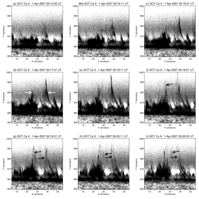
Figure 1: Chromospheric component of an X-ray and EUV coronal jet, as discussed by Sterling et al. (2010a). These are Hinode/SOT Ca ii images, where an intensity gradient filter has been applied and colors have been reversed. The scaling has been set to show the faint features that appear at the location of the coronal jet, between the two white arrows of (d). Black arrows pointing toward the left in (f-i) show a strand of the column that moves from left-to-right with time, and similarly the black arrows pointing to the right in (g-i) show a strand moving from right-to-left with time. These suggest that we are looking through a partially optically thin cylinder of material, where the cylinder is rotating. Horizontal intensity strips in the images are an artifact of the radial filter. An accompanying video shows the dynamics of the features with time. Similar figures and more details are in Sterling et al. (2010a). North is up and west to the right in this and all other solar images and movies of this paper. This video begins on 2007 April 1, 00:15:35.173 UT and ends the same day at 00:38:14.628 UT. The realtime duration is 3 seconds.

Figure 1 shows color-reversed Ca ii images of the solar limb from Hinode/SOT, showing the same feature described in Sterling et al. (2010a); this figure is similar to Figures 3 and 4 in that paper. A radial filter (due to T. E. Berger and available as sot_radial_filter.pro in the SolarSoft software package) has been applied; see Sterling et al. (2010a) for further details. We have tuned the displayed intensities to highlight faint features in the images. Nominally these Ca ii images show spicules at the limb (e.g., De Pontieu et al., 2007). From the Figure 1 images alone, it is not fully apparent whether the features indicated by the white arrows in Figure 1(d) are unrelated “type 2” spicules, or part of the same $\sim$20^′′-wide structure. Viewing the accompanying video to this figure however suggests that they are indeed part of a single entity of this size, as its coherence is maintained over 00:15:35—00:22:52 UT. In fact, they are part of the same erupting structure: Hinode/EIS 256 Å He ii images clearly show that a corresponding broad feature erupts where the Figure 1 feature occurs, and Hinode/XRT soft X-ray images confirm that this feature coincides with an X-ray jet (Sterling et al., 2010a). Because images such as those from SDO/AIA were not available in 2007 (SDO was launched in 2010), we could not confirm whether the feature that underwent eruption was a minifilament, but its basic appearance and eruptive nature (see Figs. 1(a) and 1(b) of Sterling et al., 2010a) are consistent with it being similar to the erupting minifilaments frequently observed to make jets. In any case, those Hinode images confirm that Figure 1 is showing the Ca ii-chromospheric component of a X-ray coronal jet resulting from a small-scale eruption observed in EUV. Close inspection of video accompanying Figure 1 suggests that the feature may be rotating in the Ca ii images, with the black arrows pointing to the left in Figure 1(e—h) following a strand moving from left to right, and the black arrows pointing to the right in Figure 1(6—i) following a feature moving right to left. This is consistent with the jet manifesting as a partially transparent rotating cylinder viewed from the side, in which visible strands stretch radially from the surface outward along the cylindrical jet spire, with those strands nearest the observer carried in one direction and those in the back side of the cylinder carried in the opposite direction.

We can make an estimate of the lateral velocity of the strands in the cylinder, projected against the plane of the sky. There is some uncertainty in identifying the same strands in different images, and also we cannot be certain that some strands are not separate features crossing in front of or behind the erupting feature. And, it turns out that we can find different velocities for some of the different strands. If we consider the strand pointed to by the black arrow in Figure 1(f), it moves about $8^{\prime\prime}$ over 00:18:51—00:20:53 UT, which yields a speed of $\sim$50 km s^-1. If instead however we consider the strand indicated by the right-pointing arrow in Figures 1(g)—1(i), it only moves about $2^{\prime\prime}.5$ over 00:19:31—00:20:53 UT, giving about 20 km s^-1. Other strands moving from left-to-right are closer to this lower velocity than the above-derived 50 km s^-1; nonetheless, we will just say that the estimated rotational velocities are $\sim$20—50 km s^-1 for this coronal jet. If we assume that the feature on the left side, which is the fainter of the two, is on the far side of the cylinder, and that the feature on the right side is in front, then the twisting motion would be clockwise when viewed from above.

As stated above, at the time of the Sterling et al. (2010a) paper, we had a much-less-complete understanding than now of how most coronal jets work. Much work by a number of workers have started to clarify the picture (for reviews of jets, see Raouafi et al. 2016, and the subsection authored by A. Sterling in Hinode Review Team et al. 2019). This is the probable scenario leading to the coronal jet corresponding to the chromospheric strands of Figure 1: Opposite-polarity magnetic flux elements converged at the neutral line between the two polarities, over a period lasting a couple of hours to as long as a couple of days (Panesar et al., 2017). This resulted in formation of a magnetic flux rope, perhaps containing cool minifilament material, that was rendered unstable by further convergence, and erupted to make the jet (Sterling et al., 2015). (Also see, e.g., Shen et al. 2012, Huang et al. 2012, Young & Muglach 2014, Hong et al. 2014, Adams et al. 2014, Wyper et al. 2017, McGlasson et al. 2019.) In Ca ii, apparently only the outlines of the erupting grossly cylindrical jet spire show up at locations where strands of cool material are sufficiently dense (arrows in Fig. 1).

Furthermore, the twisting motions observed in many coronal jets (e.g. Pike & Mason, 1998; Harrison et al., 2001; Patsourakos et al., 2008; Kamio et al., 2010; Raouafi et al., 2010; Curdt & Tian, 2011; Morton et al., 2012; Schmieder et al., 2013; Moore et al., 2015) plausibly might result when the minifilament field is twisted prior to eruption, and then during eruption transfers its twist via reconnection to the ambient coronal field (Moore et al., 2015; Sterling et al., 2015), a la the dynamics proposed by Shibata & Uchida (1986). The black arrows in Figure 1 might thus be showing the motions resulting from the untwisting of twist injected into the system from the erupting-minifilament field.

Curdt et al. (2012) provide a second example of a coronal jet seen in Hinode/SOT Ca ii. They observed a polar coronal jet from 2007 November 4 in X-rays with Hinode/XRT and with the Hinode/EIS spectrometer, in addition to SOT. They also observed the same jet with the SOHO/SUMER spectrometer and in EUV with STEREO/SECCHI, as described in Kamio et al. (2010). From XRT, this feature was clearly an X-ray coronal jet, and from SECCHI it was clearly a macrospicule jet in EUV 304 Å. Curdt et al. (2012) showed that this coronal jet also had a clear chromospheric counterpart in SOT images, of width $\sim$20^′′, similar to the Figure 1 case. Moreover, the EIS and SUMER spectroscopic data showed Doppler evidence that their jet was spinning. Thus, this is a second example of a coronal jet having a strand-like chromospheric counterpart, and where the spire has a twisting (or untwisting) motion.

3 High-resolution Spicules: Comparison with the Chromospheric Component of Coronal Jets

Samanta et al. (2019) observed quiet Sun spicules using ultra-high resolution adaptive optics H$\alpha$ images from the 1.6m Goode Solar Telescope (GST) at Big Bear Solar Observatory (BBSO). They observed at H$\alpha$$\pm$0.8 Å with a 0.07 Å passband of BBSO’s VIS instrument, with a diffraction-limited resolution of $\sim$0${}^{\prime\prime}.06$. Their ten-minute set of observations identified numerous bursts of clusters of narrow spicules, the enhanced spicular activities. In addition, there were a number of thin features they identified as individual spicules in the data set. They found that all 22 enhanced spicular activities that they observed with sufficient time coverage occurred in conjunction with rapidly evolving mixed-polarity magnetic flux at their bases. Thus they argued that the interactions of mixed-polarity magnetic elements was crucial in the generation of the enhanced spicular activities.

First we will look at two of these enhanced spicular activities in detail. Figure 2 (and accompanying video) shows a closeup of the first one; this is the same region as shown in panels A and D of movie S2 of Samanta et al. (2019). This was presented as an example of an enhanced spicular activity resulting from a location of flux emergence in Samanta et al. (2019), although we will reconsider this magnetic interpretation in §5. In these closeups, the enhanced spicular activity appears as a rotating cylinder, with the full width of the cylinder being approximately that between the two white arrows in Figure 2(c), a distance covering approximately $1^{\prime\prime}$. As with the macrospicule of Figure 1, this apparent cylinder appears to have strands revealing rotation of the cylinder with time. For example, the strand indicated by the black arrows in panel 2(a) and 2(b) moves toward the upper right over the time of these two panels, while the strand indicated by the blue arrow in Figures 2(a) and 2(b) moves toward the lower left over the same period; this is analogous to the black arrows in Figure 1(e—i). To estimate the velocity of the possible rotations, we measure the speed of separation of the same two strands (pointed to by the black and blue arrows in Fig. 2(b)), over the time from Figure 2(b) to Figure 2(c); the strands separate by $\sim$0${}^{\prime\prime}.39$ over the 13.8 s between those two panels, which gives $\sim$21 km s^-1.

Figure 3 (and accompanying video) shows our second detailed example from Samanta et al. (2019); this is from their case that they argued resulted from magnetic flux cancelation. Again, white arrows in Figure 3(c) show the extent of the enhanced spicular activity. In this case, spinning motion is less apparent than in the Figure 2 example. Instead, the dominant motion is a bodily shift of the entire structure upward (to the north) over, e.g., panels 3(b—c). But, although somewhat uncertain, there also appears to be some twisting of the features, visible in the relative motions of the strands pointed to by the black and blue arrows in panels 3(b—c). Over the times 4.54 to 4.66 min, the distance between the two strands contracts (with the blue-arrow strand presumably rotating around the front of the black-arrow strand) by $\sim$0.${}^{\prime\prime}17$ over 7.2 s, giving $\sim$17 km s^-1. Thus the estimated spinning speeds of the enhanced spicular activities in Figures 2 and 3 are about the same to within the uncertainty of our measurements, $\sim$20 km s^-1. This is near the lower end of the range of estimates for the twisting velocity of the jet in Figure 1.

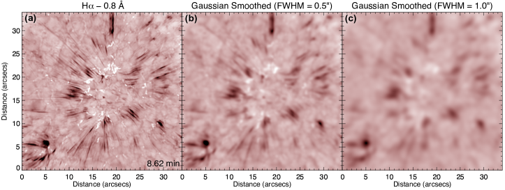
Figure 4: The spicule region studied in Samanta et al. (2019), observed at H$\alpha$-0.8 Å with BBSO/GST, from the time of Fig. 2(c). Panel (a) is a reproduction of Fig. 1(a) of that paper, but without the magnetic field. This is shown with the full GST resolution of $\sim$0${}^{\prime\prime}.06$. (b) The same images as in (a), but with a Gaussian smoothing with FWHM $0^{\prime\prime}.5$ applied. In this case, details of the enhanced spicular activities are beginning to get lost, as they blur into features of one, two, or a few linear components; this could explain the double-stranded structure of spicules reported by some observers. (c) Same as (b), but with a Gaussian smoothing with FWHM $1^{\prime\prime}.0$ applied. The enhanced spicular activities now appear to be single blurred features, similar in appearance to classical spicules/mottles of the Beckers’ era. The accompanying video shows the dynamics of the features with time. A video similar to the left-panel full-resolution video is in Samanta et al. (2019). Time is measured from the start of the observations, at 18:45:58 UT on 2017 June 19; this video covers from 0 min to 10.12 min from that time, which is the full range of observations examined in Samanta et al. (2019). The realtime duration is 3 seconds.

We have also inspected parameters of other enhanced spicular activities identified in Samanta et al. (2019). Figure 4(a) shows the full field of view of the Samanta et al. (2019) study; this reproduces Figure 1(a) of that paper, but this time with only the H$\alpha$ image, omitting the magnetic flux map. The accompanying video (left panel) shows a time sequence of the images over the entire $\sim$10 min observation window. Table 1 lists 22 enhanced spicular activities from that video, giving the $(x,y)$ coordinates of their locations (using the grid of Fig. 4), and their times as listed in the video. These selected events are the ones identified with black circles in movie S4 of Samanta et al. (2019). In the table we give the start and end time of each enhanced activity, based on our observation of it in the movie. The following column gives the difference of these times, which is the duration of the event. We then indicate whether we could observe twisting motion in the enhanced spicular activity, where ‘Y’ means that there was unambiguous apparent twisting motion (it is only “apparent” since it is based on visual inspection only, as we do not have Doppler data available). We categorize four of the events as ‘W’, indicating that we believe that there is weak or short-duration spinning (perhaps only a small fraction of a rotation), but we are more uncertain in these cases than in the ‘Y’ cases as to whether there was actual spinning. In some cases we see splitting-type of motions of the enhanced spicular activities, similar to that described elsewhere (e.g., Sterling et al. 2010b, Yurchyshyn et al. 2020), where part of the feature splits off from the body and expands away laterally; we denote this by ‘S’ when we see splitting in the absence of obvious twisting motions. We denote cases without obvious spinning or splitting with ‘N,’ and cases that were uncertain with ‘U.’ In cases where there was spinning and/or splitting (Y, S, W cases), we measured the velocity by tracking features similar to what we did for the cases of Figures 2 and 3; the penultimate column of table 1 gives the time period over which we made these measurements, and the final column gives the determined velocity along with an uncertainty based on our estimates of the accuracy of our measurements. The last row of the table gives the averages for the duration and velocity.

We find that about one-third of the events show clear visual evidence of twisting motions. Four additional ones might show weak spinning, but this is somewhat uncertain. On average the events have durations of about three minutes, but it will be recalled that this is only for the spicular events of sufficient velocity to appear in the passband defined by the GST filter centered on H$\alpha$$\pm 0.8$ Å; therefore comparisons with other measurements of durations of spicules/mottles must be made with caution. Finally, the measured twisting/splitting velocities (for the 14 cases where we could make estimates in the final column) average about 30 km s^-1, but cover a wide range, as evidenced by the large sigma value of 15 km s^-1. This velocity distribution however is bimodal, with the two spitting velocity measurements (64 and 58 km s^-1) skewing the average; with these two values removed, the mean of the remaining measured 12 spinning and suspected-weak-spinning velocities is $22.5\pm 7.2$ km s^-1.

4 Comparisons with “Classical Spicules”

We can approximate the conditions of classical spicule observations, that is, the spicules observed in chromospheric spectral lines from the ground with earlier-era methods (e.g., Beckers, 1968, 1972). Here we focus on the view of the BBSO/GST-observed spicules with spatial resolution degraded to that similar to those of earlier studies. Those earlier studies additionally often had much poorer time cadence than the 3.45 s of our GST data (Samanta et al., 2019). Furthermore, the passband (transmission profile) of the H$\alpha$ filters used previously would have been of different quality than that of the Fabry-Pérot etalon of the Samanta et al. (2019) study. Nonetheless, here we only consider consequences of degrading the spatial resolution from that of the GST’s $\sim$0${}^{\prime\prime}.06$ resolution. Pereira et al. (2013) did a similar degradation of resolution of Hinode/SOT Ca ii limb spicules, and that added support to the idea that the spicules identified as type 2 in the SOT images are the classical spicules. Here we are repeating the Pereira et al. (2013) exercise, but this time for the on-disk H$\alpha$ images we use here, in an effort to clarify the relationship between the features identified in Samanta et al. (2019) and the classical spicules.

The Figure 4(a) image, and accompanying video (left panel) shows the Samanta et al. (2019) region with full spatial resolution. Figure 4(b) (and accompanying video, middle panel) shows the same image, but with a Gaussian smoothing of FWHM $0^{\prime\prime}.5$ applied to each pixel in the image. In the same fashion, Figure 4(c) (and accompanying video, right panel) shows the same image with a Gaussian smoothing of FWHM $1^{\prime\prime}.0$ applied. Accompanying videos show corresponding time sequences of the images.

Compared to the full-resolution version, the FWHM $1^{\prime\prime}.0$ version in Figure 4(c) has lost a large amount of the structure of the enhanced spicular activities. Indeed, when viewed as a movie, these “enhanced spicular activities” display group behavior, and are likely what would have been identified as “spicules,” with widths of $\sim$1^′′, as reported by many of the earlier studies. Thus this figure and accompanying video show classical spicules (or “fine dark mottles”).

The middle-resolution version of FWHM $0^{\prime\prime}.5$ in Figure 4(b) shows the enhanced spicular activities to be only partially resolved. In many cases only the edges of the enhanced spicular activities are prominent, giving the spicules a double or twin structure, which has sometimes been reported (Tanaka, 1974; Suematsu et al., 1995; Suematsu, 1998).

Returning again to the full-resolution version in Figure 4(a), the enhanced spicular activities are resolved into striations; this is suggestive of the “2D sheet-like structure” for spicules, as described by Judge et al. (2012). It is therefore understandable that the striations could appear as sheets under high resolution. Different from Judge et al. (2012) however, we argue that many spicules could result from an upward mass flow of material, driven by an erupting microfilament undergoing reconnection with surrounding magnetic field. Sekse et al. (2013a) and Pereira et al. (2016) have already argued that the sudden appearance of sheet-like spicules could be due to transverse and/or torsional motions along the line of sight in the spicule body, and this explanation seems fully plausible.

As mentioned in the introduction, assuming that there are two spicule types, the enhanced spicular activities of Samanta et al. (2019) would likely correspond to the type 2 spicules, and therefore our findings of this section are in agreement with the conclusions of Pereira et al. (2013). Our degradation exercise here demonstrates that the on-disk features we observe here likely correspond to the limb spicules of Pereira et al. (2013), and it shows that the “enhanced spicular activities” are in fact the classical spicules/mottles, something that was not immediately apparent in the Samanta et al. (2019) study. This result might have been partially anticipated, given that Pereira et al. (2013) argued that type II spicules can be degraded to classical spicules, and that various works (e.g. Langangen et al., 2008; Rouppe van der Voort et al., 2009; Sekse et al., 2012, 2013a, 2013b) argue that RBEs/RREs are the on-disk representation of specifically type II spicules. In some cases it was suggested that a single larger RBE (e.g. Sekse et al., 2013b) or spicule (e.g. Pereira et al., 2016) might be composed of thinner strands. Our work however emphatically emphasizes this last point: we argue that the clusters of strands that make up enhanced spicular activities are plausibly part of a single larger-scale spicule structure (often of width similar to those given for classical spicules: $\sim$0^′′.5—1^′′.0), analogous to how the strands that make up the chromospheric component of the coronal jet in Figure 1 are all part of the same macroscopic EUV/X-ray coronal jet.

5 Summary and Discussion

Comparisons between high-resolution observations of spicules from BBSO/GST, and observations of the chromospheric component to coronal jets, shows that it is plausible to consider that some population of spicules could be scaled-down versions of coronal jets.

If we assume for a moment that this is that case, that is, that many spicules are miniature versions of coronal jets, then we can then explain many of the GST high-resolution observations, and we can also offer explanations for several other previously observed spicule properties. We make these arguments in the following paragraphs.

Many coronal jets result from eruption of a minifilament. It is - apparently - only some strands of the column (spire) of the jet that are visible in chromospheric images. Thus in the case of Figure 1, we see selections of cool-material strands that connect the photospheric magnetic flux with the jet-spire field that has undergone reconnection with an erupting minifilament flux rope; an appropriate erupting feature, perhaps a cool-material minifilament, is apparent in Hinode/EIS slot images, and the resulting soft X-ray jet spire is apparent in Hinode/XRT images (Sterling et al., 2010a); similarly, under our assumption, spicules, such as those in Figures 2 and 3, would be the chromospheric component – visible at the observed GST wavelength – of the spire of a miniature jet-like feature made by an erupting microfilament flux rope. Coronal jets show spin, presumably because the erupting minifilament’s field is twisted and unleashes its twist onto neighboring open (or far-reaching) field via interchange reconnection (Moore et al., 2015); spicules similarly often show twist (e.g., Pasachoff et al., 1968; De Pontieu et al., 2014), and this could result from an erupting microfilament field having twist that it imparts onto the spicule field via reconnection. Moreover, the twist velocities we estimate for the enhanced spicular activities, $\sim$20—30 km s^-1, match well with the estimated/observed spicule Doppler twist-speed values of $\sim$30 km s^-1 of Pasachoff et al. (1968) and 10—30 km s^-1 of De Pontieu et al. (2014), and similar observed transverse oscillational velocities (see, e.g., Zaqarashvili & Erdléyi, 2009), Hinode/SOT-observed limb-spicule horizontal speeds (Pereira et al., 2012), and some measurements of RBE transverse speeds (Sekse et al., 2013a).

The minifilament flux ropes that erupt to form coronal jets are apparently built up by canceling opposite-polarity magnetic fields (Panesar et al., 2017); spicules also apparently form at locations of interactions among opposite-polarity fields (Samanta et al., 2019). While for coronal jets the dominant mechanism that builds the minifilament field apparently is magnetic flux cancelation (e.g., Panesar et al., 2017; McGlasson et al., 2019), Samanta et al. (2019) on the other hand advocated both magnetic cancelation and emergence as possible causes for spicules. We caution however that the fields involved with spicule creation might be quite weak, of order 10 G or weaker. It is possible that some of the apparently emerging fields identified by Samanta et al. (2019) at the base of spicules could also have weak elements that are undergoing cancelation. Moreover, it is common for coronal jets to form at locations where the minority polarity pole of an emerging bipole cancels with surrounding majority polarity field (e.g., Shen et al., 2012; Sterling et al., 2017; Panesar et al., 2018). Thus, the enhanced spicular activity events identified in Samanta et al. (2019) as possibly resulting from emergence episodes (such as our Fig. 2 event) might in fact be prepared and triggered by cancelation instead. Even-higher-resolution magnetograms and spicule images will be required to determine whether emergence in the absence of cancelation sometimes produces spicules. (Wang et al. 1998 found evidence that flux cancelation might be responsible for some high-speed spicules.)

If erupting microfilaments produce spicules, then there would be a natural scaling with three peaks in size range for filament-like eruptions causing transient solar activity (Sterling & Moore, 2016): (i) active-region-scale filament eruptions that drive solar eruptions and CMEs, (ii) supergranule-scale minifilament eruptions resulting in coronal jets, and (iii) granule-scale microfilament eruptions that result in spicules. Thus, the three peaks in size scale for the filament-like features that erupt would reflect three natural magnetic size scales in the Sun: (i) active regions, (ii) supergranules, and (iii) granules. Moreover, magnetic flux cancelation might be the buildup and trigger mechanism for many of the eruptions in all three cases, respectively for (i) large filament eruptions (Sterling et al., 2018; Chintzoglou et al., 2019), (ii) minifilament eruptions, and (iii) microfilament eruptions.

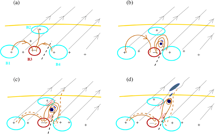
Figure 5: Schematic showing the proposed production of an enhanced spicular activity, assuming they are scaled-down versions of coronal jets that form via eruption of a microfilament flux rope built and triggered by canceling opposite-polarity magnetic fields. (a) Magnetic setup, tailored to the enhanced spicular activity of Fig. 2(a) viewed from the southeast, where the yellow curve represents the solar limb. The blue (positive) and red (negative) magnetic flux patches B1-B4 are as shown in Fig. 2(a). (B1 is not in the displayed field of view of Fig. 2, but a positive field element that could represent B1 can be seen in Fig. 1 of Samanta et al. 2019.) Plus (+) and minus (-) signs indicate polarities. Black solid lines represent open (or far-reaching) magnetic field, and the dashed black line represents a magnetic neutral line. Brown lines show the field joining the minority negative polarity element with surrounding positive field, forming an “anemone” magnetic structure (Shibata et al., 1992); the field line connecting B3 with B2 in (a) is omitted from subsequent panels for clarity. (b) A microfilament (dark filled circle) forms in a magnetic flux rope, made by the opposite-polarity fluxes converging and canceling at the neutral line. (c) The microfilament field becomes destabilized by further cancelation and erupts, and runaway magnetic reconnection occurs at the locations of the red X-es. Dashed brown lines indicate fields that are newly formed by the reconnections. (d) As the microfilament eruption continues, external reconnection (Sterling et al., 2015) expels some of the enclosed microfilament material along the newly open field lines, forming the strands (dark patches) of the enhanced spicular activity. Twist that was in the erupting microfilament flux rope has been transferred to the far-reaching spicule field, resulting in sometimes-observed (un)twisting motions in spicules. For right-handed twist in the flux rope, the resulting enhanced spicular activity spins clockwise viewed from above. This picture is analogous to the picture of Sterling et al. (2015), which was proposed to drive coronal jets such as the one in Fig. 1.

Figure 5 shows a schematic of the postulated mechanism for producing spicules via microfilament eruptions. The setup is based on the event of Figure 2, with corresponding magnetic elements labeled in Figures 2(a) and 5(a). The ambient field leans toward the right because the strong part of the supergranule network field resides northeast of the field of view of the spicule in Figure 2, which corresponds to the left in Figure 5. Figure 5(b) shows the microfilament flux rope field developing, presumably as the negative- and positive-polarity elements cancel at the magnetic neutral line. If those canceling fields are sheared, they will generate a flux rope containing twist (van Ballegooijen & Martens, 1989). Figure 5(c) shows runaway reconnection taking place below the erupting microfilament (flare-like, or “internal” reconnection, meaning internal to the erupting microfilament field) and between the erupting microfilament field and the ambient field (interchange, or “external” reconnection). These reconnections make new closed and open (or far-reaching) field lines, indicated by the dashed lines in the figure. (Corresponding reconnections are defined in the minifilament-eruption case for jets in Sterling et al. 2015.) Figure 5(d) shows when the reconnection has eaten into the microfilament flux rope, ejecting chromospheric-material microfilament material along the open field, to make the chromospheric spicule. The external reconnection transfers/injects any twist built up in the microfilament field onto the spicule field, resulting in the sometimes-observed spinning (untwisting) spicule motion. This picture is analogous to that for the minifilament-eruption mechanism for making the coronal jets (Sterling et al., 2015).

From our discussion in §4, what we are calling a “spicule” in this description could appear as an enhanced spicular activity and/or spicule sheet, a twinned spicule, or a classical spicule, depending on the observation methods and circumstances. Thus, assuming that spicules are small versions of coronal jets is also consistent with the these descriptions of spicule-scale chromospheric features.

We can understand why the medium-resolution images of Figure 4(b) show some features to appear to be double/twin spicules if a spicule is a cylindrical column where only some strands of semi-opaque cooler material show up in chromospheric lines, as we believe we are observing with the jet of Figure 1. If we assume that the semi-opaque strands are uniformly distributed around the edge of an approximately cylindrical spicule, then blurring the view (from the side-on perspective of Fig. 1) would tend to show more opaque material near the two sides of the cylinder, where the apparent density of those strands along the line of sight is highest. Thus the spicular geometry expected in the case that it is a scaled-down coronal jet could explain the sometimes-reported twinned appearance of spicules (other models might also expect a cylindrical spicule shape, in which case the same explanation could apply). Furthermore, our $\sim$1^′′-degraded-resolution images (Fig. 4(c)) show that the enhanced spicular activities of Samanta et al. (2019) resemble what were previously observed as on-disk classical spicules/mottles. This agrees with the work first done by Pereira et al. (2012) showing that some Hinode/SOT Ca ii limb spicules resemble classical spicules.

Other observers have found stranded structure of spicules that appear to be similar to what we see, but at the limb (e.g., Pereira et al., 2012, 2016). A study by Skogsrud et al. (2014) found that it is common for spicules to consist of multiple threads, with individual threads showing complex dynamics, with groups of threads showing common behavior, and with some of them displaying torsional motions; this is fully consistent with their observed features being the same as our enhanced spicular activities. Other high-resolution studies of on-disk spicules (RBEs/RREs) also show stranded structure (Yurchyshyn et al., 2020). Some of the observations of finer, individual, spicules described by Samanta et al. (2019) might be of substrands of an enhanced spicular activity, or themselves be composed of still-finer strands. Still however we cannot rule out that such individual spicules might have a different driving mechanism all together.

Other expected characteristics of a microfilament-eruption model for spicules however are not obvious in the BBSO/GST spicule observations. Many coronal jets are made by erupting minifilaments, and a brightening often appears to one side of the jet’s base. Sterling et al. (2015) called this a jet bright point (JBP), and interpreted it as a small flare arcade occurring beneath the erupting minifilament, in analogy to a typical solar flare arcade occurring beneath erupting large-scale filaments. If spicules result from the same process, then we might expect evidence of an erupting microfilament and a corresponding brightening; the small brown dashed loop at the spicule’s base in Figures 5(c, d) represents this brightening. Also expected is brightening of a neighboring bipolar lobe at the jet/spicule base; the larger dashed brown loop in Figures 5(c, d) represents this brightening. We do not however see any hints of these brightenings in the BBSO/GST data. SDO/AIA 171 Å movies of our spicule region are provided in Samanta et al. (2019) (see movies S5—S9 in that paper); they show no evidence for 171 Å  brightenings at the base in the enhanced spicular activities (classical spicules/mottles). We have inspected other AIA EUV channels, including 304, 193, and 211 Å, and also hotter-line AIA EUV channels, and we similarly find no evidence of base brightenings. As can been seen in the 171 Å movies of Samanta et al. (2019) however (and similarly for the other channels we have inspected), both the spatial resolution and the time cadence of AIA are likely too low for a complete assessment of this question. AIA UV 1600 and 1700 Å images show brightenings that closely match those of the bright filigree pattern visible in our video vid4abc, but no obvious additional brightening, given the resolution and cadence. Thus the question of possible UV/EUV spicule base brightenings will have to be reconsidered with substantially higher resolution and cadence instruments in the future. (Panesar et al. 2019 and Sterling et al. 2020 find transient brightenings in high-resolution Hi-C 172 Å EUV images at the base of some small-scale features, but it is not yet known how those EUV jets relate to typical spicules.)

More generally, we know of no clear, unambiguous such brightenings occurring near the time of spicule initiation; Suematsu et al. (1995) reported brightenings that tend to begin at the time of peak spicule extension or later, and so perhaps too late to correspond to the JBP. Sterling et al. (2010b) reported weak brightenings in Hinode/SOT Ca ii near-limb spicule images, which might be candidates for JBP counterparts if they can be confirmed. While the lack of clear brightenings near the base of spicules in the far wings of H$\alpha$ could be an argument that spicules are not due to microfilament eruptions, at the same time we note that the JBP is not apparent in the chromospheric images of Figure 1, even though it is visible in XRT X-ray images at comparable times (Sterling et al., 2010a, Fig. 1(k,l)). For that Figure 1 jet we do not know whether the erupting features (the suspected minifilament) would have been seen in Ca ii, because the SOT observations for this event started after the eruption visible in EIS had taken place.

A possibility however is that both an erupting microfilament and corresponding brightenings might not be easily observable in high-core-opacity chromospheric spectral lines such as H$\alpha$. This is because the putative erupting microfilament might might have a very slow velocity while it is still rising as part of an in-tact flux rope, and the brightening features similarly might be stationary or moving very slowly. In that case, they might not be visible in our line-wing images at H$\alpha$-0.8 Å. Also, such an erupting microfilament and brightenings would be expected to form in the upper photosphere or low chromosphere, near where the photospheric fields are canceling. Observations near the center of the line, which would show low-velocity features, show emission from features higher in the chromosphere, with lower-height features not visible due to high opacity. Therefore any potential erupting microfilaments might be “hiding” at wavelengths near the H$\alpha$-line core! In our data, we have identified a couple of candidate absorption features that might be erupting microfilaments that are just beginning to move rapidly enough to appear in the H$\alpha$-0.8 Å images; green arrows in the bottom panels of Figures 2(c) and 3(a) show these features. It would be valuable to look for such features with high-resolution, high-cadence images at several locations in the H$\alpha$ line, together with high-quality magnetograms. Such a project might be attempted at the BBSO/GST, the Swedish Solar Telescope, the New Vacuum Solar Telescope, or with the upcoming DKIST facility.

The Samanta et al. (2019) observations of spicules makes it hard to see how they could be driven by shock waves produced by photospheric motions, because mixed-polarity magnetic field seems to be required to generate these spicules. Numerical simulations had been pointing to this conclusion for some time (e.g. Sterling & Mariska, 1990; Martínez-Sykora et al., 2013). (Whether such shocks drive the features seen in plages called type 1 spicules (De Pontieu et al. 2007), or anemone jets (Shibata et al. 2007), is a different question, one that we will not address here.) Similarly, Alfvén waves that are generated by photospheric motions alone would not seem capable of producing the 20 km s^-1 torsional motions that we observe in the low chromosphere (Hollweg et al., 1982; Kudoh & Shibata, 1999). If however the source of the torsional motions is something different (perhaps an erupting twisted microfilament flux rope imparting its twist onto the spicule field, as envisioned in Fig. 5), then a larger Alfvén-wave amplitude might naturally result. Inputing such larger-amplitude Alfvén waves at the base of the chromosphere might be a future direction for exploration in Alfvén-wave-driven spicule models (e.g. Iijima & Yokoyama, 2017).

Also, Martínez-Sykora et al. (2017) were able to simulate so-called type II spicules by including ambipolar diffusion processes in a solar atmosphere model. It appears that their model spicules result when flux tubes that are contorted by the high-beta plasma in and below the photosphere spring from the photosphere into the chromosphere. Those contortions are released via ambipolar diffusion of the field through the plasma, and the resulting upward whipping motion of the field can eject material upward as the spicule. It is still to be determined whether this proposed mechanism is consistent with high-resolution spicule and magnetic-field observations, such as those of Samanta et al. (2019). More generally, new observations may support that more than one mechanism can produce what we call “spicules.” From table 1, of the 22 enhanced spicular activities: seven show what we regard as clear visual evidence for spinning motions, four are somewhat uncertain but might show weak spinning, another four show clear evidence for splitting, and seven (including one of the splitting ones) are uncertain regarding whether they spin (meaning that we could not determine with enough confidence to make a judgment). Only one event (event 10) appeared to us not to have either spinning or splitting behavior. If only the spinning, weakly spinning, and splitting events are due to minifilament eruptions, then about one-half of the enhanced spicular activities could be due to something else. Additionally, Samanta et al. (2019) identified numerous “individual” or isolated spicules (probably equivalent to the “isolated RBEs” of Sekse et al., 2012)), and it is uncertain whether those isolated spicules are driven by the same mechanism as the “enhanced spicular activity” spicules. Moreover, our observations are limited only to the subset of spicules that are prominent in our limited observing range (H$\alpha$$\pm 0.8$ Å, corresponding to $\sim\pm$36 km s^-1), and therefore our observations may omit a substantial portion of the spicule population. Future observations should help clarify whether multiple mechanisms drive spicules.

Table 1: “Enhanced Spicular Activity” Properties

Event	Location [($x,y$)]	Time Period	Duration [min]	Twist?	Measurement Period	Velocity [km s-1]
1	(14,19)	— — 2.42	—	U	—	—
2	(22,23)	— — 2.24	—	Y	1.26 — 1.96	$14\pm 2$
3	(28,18)	0.34 — 2.36	2.02	Y	1.78 — 2.24	$30\pm 3$
4	(19,14)	0.17 — 2.59	2.42	S	0.75 — 1.44	$64\pm 10$
5	(23,21)	1.61 — 5.00	3.39	W	4.43 — 5.00	$34\pm 5$
6	(20,11)	1.73 — 4.95	3.22	S	2.93 — 3.34	$29\pm 3$
7	(13,17)	0.34 — 4.95	4.61	Y	2.53 — 2.88	$21\pm 2$
8	(12,20)	2.88 — 4.95	2.07	S	—	—
9	(29,19)	2.47 — 5.12	2.65	W	2.82 — 3.28	$16\pm 3$
10	(30,16)	3.28 — 5.06	1.78	N	—	—
11 (Fig. 3)	(19,28)	4.14 — 5.29	1.15	W	4.54 — 4.66	$17\pm 2$
12	(12,15)	4.20 — 5.75	1.55	U	—	—
13 (Fig. 2)	(15,21)	3.62 — 9.37	5.75	Y	7.88 — 8.11	$21\pm 2$
14	(28,20)	6.56 — 9.14	2.58	U	—	—
15	(21,12)	6.15 — 9.32	3.17	Y	7.65 — 8.05	$33\pm 3$
16	(14,16)	8.05 — 9.83	1.78	W	9.43 — 9.72	$16\pm 3$
17	(29,10)	8.22 — —	—	Y	8.68 — 9.03	$22\pm 3$
18	(27,16)	8.62 — —	—	Y	8.68 — 9.03	$17\pm 3$
19	(18,11)	8.85 — —	—	U/S	9.83 — 10.12	$58\pm 15$
20	(14,16)	9.03(?)— 9.83	—	U	—	—
21	(23,18)	8.85 — —	—	U	—	—
22	(16,20)	9.03 — —	—	U	—	—
Averages	—	—	$2.72\pm 1.2$	—	—	$28.0\pm 15.5$

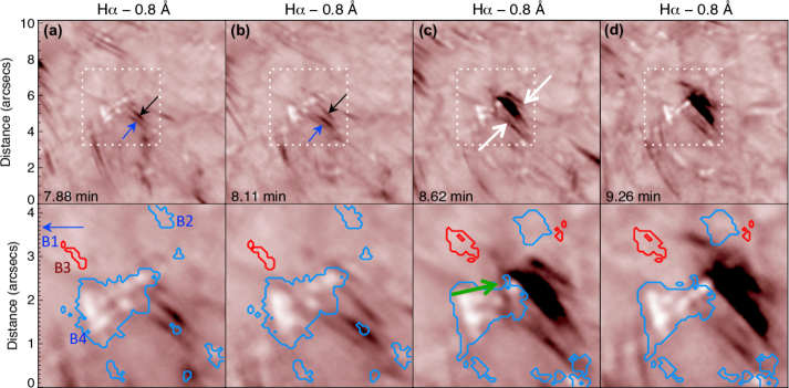
Figure 2: Close up of an “enhanced spicular activity” identified in BBSO/GST observations of Samanta et al. (2019). This is from Fig. 2a of that paper. For each of (a—c), the top panel is a $9^{\prime\prime}.3$ square region, and the bottom panel is a close up of the top panel’s dashed white box, and has size $4^{\prime\prime}.3$ square. In (c), the white arrows show the approximate lateral extent (width) of the enhanced spicular activity. In (a-b), the black arrow points to a strand that moves toward the upper right with time, in a direction opposite to the that of the strand pointed to by the blue arrows in those panels; these mutual motions suggest that the enhanced spicular activity feature is undergoing rotation, analogous to that inferred for the chromospheric manifestation of the coronal jet in Fig. 1. The green arrow in the bottom panel of (c) shows an upward-moving horizontally oriented feature that is a candidate for an erupting microfilament, which may have been formed by flux cancelation between negative and positive-polarity magnetic fields (respectively, red and blue contours in bottom panels), and eruption of which might produce the enhanced spicular activity. B1-B4 in (a) mark magnetic polarities discussed in Fig. 5. Fig. 4 shows this event at the time of 2(c); it is in the southwest of the field of view, near location (21 Mm,7.5 Mm) in those panels. An accompanying video shows the dynamics of the features with time. A similar video appears in Samanta et al. (2019). In these and in other BBSO/GST images and movies, time is measured from the start of the observations, at 18:45:58 UT on 2017 June 19; this video covers from 4.26 min to 10.12 min from that time. The realtime duration of the video is 3 seconds.

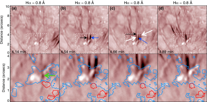
Figure 3: Same as Fig. 2, but for the enhanced spicular activity of Fig. 2(c) in Samanta et al. (2019). Again the white arrows in (c) indicate the width of the enhanced spicular activity. In this case the entire enhanced spicular activity whips upward with time, and there also appears to be relative rotation of the two strands pointed to by the black and blue arrows of panels (b) and (c). In the bottom panel of (a), the green arrow points to a possible erupting microfilament. An accompanying video shows the dynamics of the features with time. A similar video appears in Samanta et al. (2019). Time is measured from the start of the observations, at 18:45:58 UT on 2017 June 19; this video covers from 2.19 min to 7.47 min from that time. Its realtime duration is 3 seconds.

References

- Adams et al. (2014) Adams, M., Sterling, A. C., Moore, R. L., & Gary, G. A. 2014, Astrophysical Journal, 783, 11, doi: 10.1088/0004-637X/783/1/11
- Athay (1959) Athay, R. G. 1959, Astrophysical Journal, 129, 164, doi: 10.1086/146603
- Beckers (1968) Beckers, J. M. 1968, Solar Physics, 3, 367, doi: 10.1007/BF00171614
- Beckers (1972) —. 1972, Annual Review of Astronomy and Astrophysics, 10, 73, doi: 10.1146/annurev.aa.10.090172.000445
- Bradshaw & Klimchuk (2015) Bradshaw, S. J., & Klimchuk, J. A. 2015, Astrophysical Journal, 811, 129, doi: 10.1088/0004-637X/811/2/129
- Bray & Loughhead (1974) Bray, R. J., & Loughhead, R. E. 1974, The Solar Chromosphere (London: Chapman and Hall)
- Chintzoglou et al. (2019) Chintzoglou, G., Zhang, J., Cheung, M. C. M., & Kazachenko, M. 2019, ApJ, 871, 67, doi: 10.3847/1538-4357/aaef30
- Cirtain et al. (2007) Cirtain, J. W., Golub, L., Lundquist, L., et al. 2007, Science, 318, 1580, doi: 10.1126/science.1147050
- Curdt & Tian (2011) Curdt, W., & Tian, H. 2011, Astronomy and Astrophysics, 532, L9, doi: https://doi.org/10.1051/0004-6361/201117116
- Curdt et al. (2012) Curdt, W., Tian, H., & Kamio, S. 2012, Solar Physics, 280, 417, doi: 10.1007/s11207-012-9940-9
- De Pontieu et al. (2012) De Pontieu, B., Carlsson, M., Rouppe van der Voort, L. H. M., et al. 2012, Astrophysical Journal, 752L, 12, doi: 10.1088/2041-8205/752/1/L12
- De Pontieu et al. (2004) De Pontieu, B., Erdélyi, R., & James, S. P. 2004, Nature, 430, 536, doi: 10.1038/nature02749
- De Pontieu et al. (2011) De Pontieu, B., McIntosh, S. W., Carlsson, M., et al. 2011, Science, 331, 55, doi: 10.1126/science.1197738
- De Pontieu et al. (2007) De Pontieu, B., McIntosh, S., Hansteen, V. H., et al. 2007, Publications of the Astronomical Society of Japan, 59, 655, doi: 10.1093/pasj/59.sp3.S655
- De Pontieu et al. (2014) De Pontieu, B., Rouppe van der Voort, L., McIntosh, S. W., et al. 2014, Science, 346, 1255732, doi: 10.1126/science.1255732
- Harrison et al. (2001) Harrison, R. A., Bryans, P., & Bingham, R. 2001, Astronomy & Astrophysics, 379, 324, doi: 10.1051/0004-6361:20011171
- Henriques et al. (2016) Henriques, V. M. J., Kuridze, D., Mathioudakis, M., & Keenan, F. P. 2016, Astrophysical Journal, 820, 124, doi: 10.3847/0004-637X/820/2/124
- Hinode Review Team et al. (2019) Hinode Review Team, Khalid, A.-J., Patrick, A., et al. 2019, Publications of the Astronomical Society of Japan, 71, id.R1, doi: 10.1093/pasj/psz084
- Hollweg (1992) Hollweg, J. V. 1992, Astrophysical Journal, 257, 345, doi: 10.1086/159993
- Hollweg et al. (1982) Hollweg, J. V., Jackson, S., & Galloway, D. 1982, Solar Physics, 75, 35, doi: 10.1007/BF00153458
- Hong et al. (2014) Hong, J., Jiang, Y., Yang, J., et al. 2014, Astrophysical Journal, 796, 73, doi: 10.1088/0004-637X/796/2/73
- Huang et al. (2012) Huang, Z., Madjarska, S., M., Doyle, J. G., & Lamb, D. A. 2012, Astronomy and Astrophysics, 548, 62, doi: 10.1051/0004-6361/201220079
- Iijima & Yokoyama (2017) Iijima, H., & Yokoyama, T. 2017, Astrophysical Journal, 848, 38, doi: 10.3847/1538-4357/aa8ad1
- Judge et al. (2012) Judge, P. G., Reardon, K., & Cauzzi, G. 2012, ApJ, 755, 11, doi: 10.1088/2041-8205/755/1/L11
- Kamio et al. (2010) Kamio, S., Curdt, W., Teriaca, L., Inhester, B., & Solanki, S. K. 2010, Astronomy and Astrophysics, 510, 1, doi: 10.1051/0004-6361/200913269
- Klimchuk (2012) Klimchuk, J. A. 2012, Journal of Geophysical Research, 117, A12102, doi: 10.1029/2012JA018170
- Klimchuk & Bradshaw (2014) Klimchuk, J. A., & Bradshaw, S. J. 2014, Astrophysical Journal, 791, 60, doi: 10.1088/0004-637X/791/1/60
- Kudoh & Shibata (1999) Kudoh, T., & Shibata, K. 1999, Astrophysical Journal, 514, 493, doi: 10.1086/306930
- Langangen et al. (2008) Langangen, O., De Pontieu, B., Carlsson, M., et al. 2008, Astrophysical Journal, 679, 167L, doi: 10.1086/589442
- Lee et al. (2000) Lee, C.-Y., Chae, J., & Wang, H. 2000, Astrophysical Journal, 545, 1124, doi: 10.1086/317821
- Lynch et al. (1973) Lynch, D. K., Beckers, J. M., & Dunn, R. B. 1973, Solar Physics, 30, 63L, doi: 10.1007/BF00156173
- Madjarska et al. (2011) Madjarska, M. S., Vanninathan, K., & Doyle, J. G. 2011, Astronomy and Astrophysics, 532, L1, doi: 10.1051/0004-6361/201116735
- Martínez-Sykora et al. (2017) Martínez-Sykora, J., De Pontieu, B., Hansteen, V. H., et al. 2017, Science, 356, 1269, doi: 10.1126/science.aah5412
- Martínez-Sykora et al. (2013) Martínez-Sykora, J., De Pontieu, B., Leenaarts, J., et al. 2013, Astrophysical Journal, 771, 66, doi: 10.1088/0004-637X/771/1/66
- McGlasson et al. (2019) McGlasson, R. A., Panesar, N. K., Sterling, A. C., & Moore, R. L. 2019, ApJ, 882, 16, doi: 10.3847/1538-4357/ab2fe3
- Michard (1974) Michard, R. 1974, in Proceedings from IAU Symposium no. 56 held at Surfer’s Paradise, Qld., Australia, 3-7 September 1973. Edited by R. Grant Athay. International Astronomical Union. Symposium no. 56, ed. R. G. Athay (Dordrecht; Boston: Reidel), 3
- Moore (1990) Moore, R. L. 1990, Società Astronomica Italiana, Memorie (MmSAI), 61, 317
- Moore et al. (2011) Moore, R. L., Sterling, A. C., Cirtain, J. W., & Falconer, D. A. 2011, Astrophysical Journal, 731L, 18, doi: 10.1088/2041-8205/731/1/L18
- Moore et al. (2015) Moore, R. L., Sterling, R. L., & Falconer, D. A. 2015, Astrophysical Journal, 806, 11, doi: 10.1088/0004-637X/806/1/11
- Moore et al. (1977) Moore, R. L., Tang, F., Bohlin, J. D., & Golub, L. 1977, Astrophysical Journal, 218, 286, doi: 10.1086/155681
- Morton et al. (2012) Morton, R. J., Srivastava, A. K., & Erdélyi, R. 2012, Astronomy & Astrophysics, 542, 70, doi: 10.1051/0004-6361/201117218
- Panesar et al. (2017) Panesar, N. K., Sterling, A. C., & Moore, R. L. 2017, Astrophysical Journal, 844, 131, doi: 10.3847/1538-4357/aa7b77
- Panesar et al. (2018) —. 2018, Astrophysical Journal, 853, 189, doi: 10.3847/1538-4357/aaa3e9
- Panesar et al. (2016) Panesar, N. K., Sterling, A. C., Moore, R. L., & Chakrapani, P. 2016, Astrophysical Journal, 832L, 7, doi: 10.3847/2041-8205/832/1/L7
- Panesar et al. (2019) Panesar, N. K., Sterling, A. C., Moore, R. L., et al. 2019, Astrophysical Journal, 887L, 8, doi: 10.3847/2041-8213/ab594a
- Pasachoff et al. (2009) Pasachoff, J. M., Jacobson, W. A., & Sterling, A. C. 2009, Solar Physics, 260, 59, doi: 10.1007/s11207-009-9430-x
- Pasachoff et al. (1968) Pasachoff, J. M., Noyes, R. W., & Beckers, J. M. 1968, Solar Physics, 5, 131, doi: 10.1007/BF00147962
- Patsourakos et al. (2008) Patsourakos, S., Pariat, E., Vourlidas, A., Antiochos, S. K., & Wuelser, J. P. 2008, Astrophysical Journal, 680, L73, doi: 10.1086/589769
- Pereira et al. (2012) Pereira, T. M. D., De Pontieu, B., & Carlsson, M. 2012, Astrophysical Journal, 759, 18, doi: 10.1088/0004-637X/759/1/18
- Pereira et al. (2013) —. 2013, Astrophysical Journal, 764, 69, doi: 10.1088/0004-637X/764/1/69
- Pereira et al. (2016) Pereira, T. M. D., Rouppe van der Voot, L., & Carlsson, M. 2016, Astrophysical Journal, 824, 65, doi: 10.3847/0004-637X/824/2/65
- Pike & Mason (1998) Pike, C. D., & Mason, H. E. 1998, Solar Physics, 182, 333, doi: 10.1023/A:1005065704108
- Raouafi et al. (2010) Raouafi, N.-E., Georgoulis, M. K., Rust, D. M., & Bernasconi, P. N. 2010, Astrophysical Journal, 718, 981, doi: 10.1088/0004-637X/718/2/981
- Raouafi et al. (2016) Raouafi, N. E., Patsourakos, S., Pariat, E., et al. 2016, Space Science Reviews, 201, 1, doi: 10.1007/s11214-016-0260-5
- Rouppe van der Voort et al. (2009) Rouppe van der Voort, L., Leenaarts, J., de Pontieu, B., Carlsson, M., & Vissers, G. 2009, Astrophysical Journal, 705, 272, doi: 10.1088/0004-637X/705/1/272
- Rutten (2007) Rutten, R. J. 2007, in The Physics of Chromospheric Plasmas ASP Conference Series, Proceedings of the conference held 9-13 October, 2006 at the University of Coimbra in Coimbra, Portugal.. San Francisco, ed. P. Heinzel, I. Dorotovic̆, & R. J. Rutten (San Francisco: Astronomical Society of the Pacific), 27
- Samanta et al. (2015) Samanta, T., Pant, V., & Banerjee, D. 2015, Astrophysical Journal, 815, L16, doi: 10.1088/2041-8205/815/1/L16
- Samanta et al. (2019) Samanta, T., Tian, H., Yurchyshyn, V., et al. 2019, Science, 366, 890, doi: 10.1126/science.aaw2796
- Savcheva et al. (2007) Savcheva, A., Cirtain, J., Deluca, E. E., et al. 2007, Publications of the Astronomical Society of Japan, 59, 771, doi: 10.1093/pasj/59.sp3.S771
- Schmieder et al. (2013) Schmieder, B., Guo, Y., Moreno-Insertis, F., et al. 2013, Astronomy and Astrophysics, 559, A1, doi: 10.1051/0004-6361/201322181
- Secchi (1877) Secchi, A. 1877, Le Soleil, Vol. 2 (Paris: Gauthier-Villars)
- Sekse et al. (2012) Sekse, D. H., Rouppe van der Voort, L., & De Pontieu, B. 2012, Astrophysical Journal, 752, 108, doi: 10.1088/0004-637X/752/2/108
- Sekse et al. (2013a) —. 2013a, Astrophysical Journal, 764, 164, doi: 10.1088/0004-637X/764/2/164
- Sekse et al. (2013b) Sekse, D. H., Rouppe van der Voort, L., De Pontieu, B., & Scullion, E. 2013b, Astrophysical Journal, 769, 44, doi: 10.1088/0004-637X/769/1/44
- Shen et al. (2012) Shen, Y., Liu, Y., Su, J., & Deng, Y. 2012, Astrophysical Journal, 745, 164, doi: 10.1088/0004-637X/745/2/164
- Shibata et al. (1992) Shibata, K., Ishido, Y., Acton, L. W., Strong, K. T.and Hirayama, T., & Uchida, Y. 1992, PASJ, 2, 173
- Shibata & Uchida (1986) Shibata, K., & Uchida, Y. 1986, Solar Physics, 178, 379
- Shibata et al. (2007) Shibata, K., Nakamura, T., Matsumoto, T., et al. 2007, Science, 318, 1591, doi: 10.1126/science.1146708
- Shimojo et al. (1996) Shimojo, M., Hashimoto, S., Shibata, K., et al. 1996, Publications of the Astronomical Society of Japan, 48, 123, doi: 10.1093/pasj/48.1.123
- Skogsrud et al. (2014) Skogsrud, H., Rouppe van der Voort, L., & De Pointieu, D. 2014, Astrophysical Journal, 795, 23, doi: 10.1088/2041-8205/795/1/L23
- Skogsrud et al. (2015) Skogsrud, H., Rouppe van der Voort, L., De Pointieu, D., & Pereira, T. M. D. 2015, Astrophysical Journal, 806, 170, doi: 10.1088/0004-637X/806/2/170
- Sterling (2000) Sterling, A. C. 2000, Solar Physics, 196, 79, doi: 10.1023/A:1005213923962
- Sterling et al. (2010a) Sterling, A. C., Harra, L. K., & Moore, R. L. 2010a, Astrophysical Journal, 722, 1644, doi: 10.1088/0004-637X/722/2/1644
- Sterling & Mariska (1990) Sterling, A. C., & Mariska, J. T. 1990, Astrophysical Journal, 349, 647, doi: 10.1086/168352
- Sterling & Moore (2016) Sterling, A. C., & Moore, R. L. 2016, Astrophysical Journal, 828, L9, doi: 10.3847/2041-8205/828/1/L9
- Sterling et al. (2010b) Sterling, A. C., Moore, R. L., & DeForest, C. E. 2010b, Astrophysical Journal, 714L, 1, doi: 10.1088/2041-8205/714/1/L1
- Sterling et al. (2015) Sterling, A. C., Moore, R. L., Falconer, D. A., & Adams, M. 2015, Nature, 523, 437, doi: 10.1038/nature14556
- Sterling et al. (2017) Sterling, A. C., Moore, R. L., Falconer, D. A., Panesar, N. K., & Martinez, F. 2017, Astrophysical Journal, 844, 28, doi: 10.3847/1538-4357/aa7945
- Sterling et al. (2018) Sterling, A. C., Moore, R. L., & Panesar, N. K. 2018, Astrophysical Journal, 864, 68, doi: 10.3847/1538-4357/aad550
- Sterling et al. (2020) Sterling, A. C., Moore, R. L., Panesar, N. K., et al. 2020, Astrophysical Journal, 889, 187, doi: 10.3847/1538-4357/ab5dcc
- Sterling et al. (1993) Sterling, A. C., Shibata, K., & Mariska, J. T. 1993, Astrophysical Journal, 407, 778, doi: 10.1086/172559
- Suematsu (1998) Suematsu, Y. 1998, in Solar Jets and Coronal Plumes, Proceedings of an International meeting, Guadeloupe, France, 23-26 February 1998, ESA, Vol. 42, ed. T.-D. Guyenne (Paris: European Space Agency (ESA)), 19
- Suematsu et al. (2008) Suematsu, Y., Ichimoto, K., Katsukawa, Y., et al. 2008, in First Results From Hinode ASP Conference Series, Vol. 397, Proceedings of the conference held 20-24 August, 2007, at Trinity College Dublin, Dublin, Ireland., ed. S. A. Matthews, J. M. Davis, & L. K. Harra (San Francisco: Astronomical Society of the Pacific), 27
- Suematsu et al. (1982) Suematsu, Y., Shibata, K., Nishikawa, T., & Kitai, R. 1982, Solar Physics, 75, 99, doi: 10.1007/BF00153464
- Suematsu et al. (1995) Suematsu, Y., Wang, H., & Zirin, H. 1995, Astrophysical Journal, 450, 411, doi: 10.1086/176151
- Tanaka (1974) Tanaka, K. 1974, in Chromospheric Fine Structure: Proceedings from IAU Symposium no. 56 held at Surfer’s Paradise, Qld., Australia, 3-7 September 1973., ed. R. G. Athay (Dordrecht; Boston: International Astronomical Union), 239
- Tavabi et al. (2015) Tavabi, E., Koutchmy, S., Ajabshirizadeh, A., Ahangarzadeh Maralani, A. R., & Zeighami, S. 2015, Astronomy & Astrophysics, 573, 7, doi: 10.1051/0004-6361/201423385
- Tian et al. (2014) Tian, H., DeLuca, E. E., Cranmer, S. R., et al. 2014, Science, 346, doi: 10.1126/science.1255711
- Tsiropoula et al. (2012) Tsiropoula, G., Tziotziou, K., Kontogiannis, I., et al. 2012, Space Science Reviews, 169, 181, doi: 10.1007/s11214-012-9920-2
- van Ballegooijen & Martens (1989) van Ballegooijen, A. A., & Martens, P. C. H. 1989, Astrophysical Journal, 343, 971, doi: 10.1086/167766
- Wang et al. (1998) Wang, H., Johannesson, A., Stage, M., Lee, C., & Zirin, H. 1998, Solar Physics, 178, 55, doi: 10.1038/nature22050
- Wyper et al. (2017) Wyper, P. F., Antiochos, S. K., & DeVore, C. R. 2017, Nature, 544, 452, doi: 10.1038/nature22050
- Young & Muglach (2014) Young, P. R., & Muglach, K. 2014, Solar Physics, 289, 3313, doi: 10.1007/s11207-014-0484-z
- Yurchyshyn et al. (2020) Yurchyshyn, V., Cao, W., Abramenko, V., Yang, X., & Cho, K.-S. 2020, Astrophysical Journal Letters, 891, 21, doi: 10.3847/2041-8213/ab7931
- Zaqarashvili & Erdléyi (2009) Zaqarashvili, T. V., & Erdléyi, R. 2009, Solar Physics, 149, 355, doi: 10.1007/s11214-009-9549-y
- Zhang et al. (2012) Zhang, Y. Z., Shibata, K., Wang, J. X., et al. 2012, Astrophysical Journal, 750, 16, doi: 10.1088/0004-637X/750/1/16
- Zirin (1988) Zirin, H. 1988, Astrophysics of the Sun (Cambridge and New York: Cambridge University Press)