Photochemistry of Anoxic Abiotic Habitable Planet Atmospheres: Impact of New H₂O Cross-Sections

Abstract

We present a study of the photochemistry of abiotic habitable planets with anoxic CO₂-N₂ atmospheres. Such worlds are representative of early Earth, Mars and Venus, and analogous exoplanets. H₂O photodissociation controls the atmospheric photochemistry of these worlds through production of reactive OH, which dominates the removal of atmospheric trace gases. The near-UV (NUV; $>200$ nm) absorption cross-sections of H₂O play an outsized role in OH production; these cross-sections were heretofore unmeasured at habitable temperatures ($<373$ K). We present the first measurements of NUV H₂O absorption at $292$ K, and show it to absorb orders of magnitude more than previously assumed. To explore the implications of these new cross-sections, we employ a photochemical model; we first intercompare it with two others and resolve past literature disagreement. The enhanced OH production due to these higher cross-sections leads to efficient recombination of CO and O₂, suppressing both by orders of magnitude relative to past predictions and eliminating the low-outgassing “false positive” scenario for O₂ as a biosignature around solar-type stars. Enhanced [OH] increases rainout of reductants to the surface, relevant to prebiotic chemistry, and may also suppress CH₄ and H₂; the latter depends on whether burial of reductants is inhibited on the underlying planet, as is argued for abiotic worlds. While we focus on CO₂-rich worlds, our results are relevant to anoxic planets in general. Overall, our work advances the state-of-the-art of photochemical models by providing crucial new H₂O cross-sections and resolving past disagreement in the literature, and suggests that detection of spectrally active trace gases like CO in rocky exoplanet atmospheres may be more challenging than previously considered.

1 Introduction

The statistical finding that rocky, temperate exoplanets are common (Dressing & Charbonneau, 2015) has received dramatic validation with the discovery of nearby potentially-habitable worlds like LHS-1140b, TRAPPIST-1e, TOI-700d, and Kepler-442b (Dittmann et al., 2017; Gillon et al., 2017; Gilbert et al., 2020; Torres et al., 2015). Upcoming facilities such as the James Webb Space Telescope (JWST), the Extremely Large Telescopes (ELTs), and the HabEx and LUVOIR mission concepts will have the ability to detect the atmospheres of such worlds, and possibly characterize their atmospheric compositions (Rodler & López-Morales, 2014; Fujii et al., 2018; Lustig-Yaeger et al., 2019; LUVOIR Team, 2019; Meixner et al., 2019; Gaudi et al., 2020).

The prospects for rocky exoplanet atmospheric characterization have lead to extensive photochemical modelling of their potential atmospheric compositions, with emphasize on constraining the possible concentrations of spectroscopically active trace gases like CO, O₂, and CH₄. Particular emphasis has been placed on modelling the atmospheres of habitable but abiotic planets with anoxic, CO₂-N₂ atmospheres (e.g., Segura et al. 2007; Hu et al. 2012; Rugheimer et al. 2015; Rimmer & Helling 2016; Schwieterman et al. 2016; Harman et al. 2018; James & Hu 2018; Hu et al. 2020). Such atmospheres are expected from outgassing on habitable terrestrial worlds, are representative of early Earth, Mars and Venus (Kasting, 1993; Wordsworth, 2016; Way et al., 2016), and are expected on habitable exoplanets orbiting younger, fainter stars or at the outer edges of their habitable zones (e.g., TRAPPIST-1e; Kopparapu et al. 2013; Wolf 2017).

Water vapor plays a critical role in the photochemistry of such atmospheres, because in anoxic abiotic atmospheres, H₂O photolysis is the main source of the radical OH, which is the dominant sink of most trace atmospheric gases (Rugheimer et al., 2015; Harman et al., 2015). Most water vapor is confined to the lower atmosphere due to the decline of temperature with altitude and the subsequent condensation of H₂O, the “cold trap” (e.g., Wordsworth & Pierrehumbert 2013). In CO₂-rich atmospheres, this abundant lower atmospheric H₂O is shielded from UV photolysis at FUV wavelengths ($\leq 200$ nm), meaning that NUV ($>200$ nm) absorption plays an overweight role in H₂O photolysis (Harman et al., 2015). Therefore, the NUV absorption cross-sections of H₂O are critical inputs to photochemical modelling of anoxic abiotic habitable planet atmospheres. However, to our knowledge, the NUV absorption of H₂O at habitable temperatures ($<373$ K) was not known prior to this work. In the absence of measurements, photochemical models relied upon varying assumptions regarding H₂O NUV absorption (Kasting & Walker, 1981; Sander et al., 2011; Rimmer & Helling, 2016; Rimmer & Rugheimer, 2019).

In this paper, we present the first-ever measurements of the NUV cross-sections of H₂O(g) at temperatures relevant to habitable worlds ($T=292\text{K}<373$ K), and explore the implications for the atmospheric photochemistry of abiotic habitable planets with anoxic CO₂-N₂ atmospheres orbiting Sun-like stars. We begin by briefly reviewing the photochemistry of anoxic CO₂-N₂ atmospheres, and the key role of H₂O (Section 2). We proceed to measure the cross-sections of H₂O(g) in the laboratory, and find it to absorb orders of magnitude more in the NUV than previously assumed by any model; this laboratory finding is consistent with our (limited) theoretical understanding of the behaviour of the water molecule (Section 3). We incorporate these new cross-sections into our photochemical model. Previous models of such atmospheres have been discordant; we conduct an intercomparison between three photochemical models to successfully reconcile this discordance to within a factor of $2\times$ (Section 4). We explore the impact of our newly measured, larger H₂O cross-sections and their concomitantly higher OH production on the atmospheric photochemistry and composition for our planetary scenario (Section 5). We focus on O₂ and especially CO, motivated by their spectral detectability and proposed potential to discriminate the presence of life on exoplanets (Snellen et al., 2010; Brogi, M. et al., 2014; Rodler & López-Morales, 2014; Wang et al., 2016; Schwieterman et al., 2016; Meadows et al., 2018; Krissansen-Totton et al., 2018; Schwieterman et al., 2019), but we consider the implications for other species as well, and especially CH₄ and H₂. We summarize our findings in Section 6. The Appendices contain supporting details: Appendix A details our simulation parameters, Appendix B details the boundary conditions, and Appendix C details our model intercomparison and the insights derived thereby. While we focus here on CO₂-rich atmospheres, our results are relevant to any planetary scenario in which H₂O photolysis is the main source of OH, which includes most anoxic atmospheric scenarios.

2 Photochemistry of CO₂-Rich Atmospheres

In this section, we briefly review the photochemistry of CO₂-rich atmospheres. For a more detailed discussion, we refer the reader to Catling & Kasting (2017).

UV light readily dissociates atmospheric CO₂ via $CO_{2}+h\nu\rightarrow CO+O$ ($\lambda<202$ nm; Ityaksov et al. 2008). The direct recombination of CO and O is spin forbidden and slow, and the reaction $O+O+M\rightarrow O_{2}+M$ is faster. Consequently, CO₂ on its own is unstable to conversion to CO and O₂ (Schaefer & Fegley, 2011). However, OH can react efficiently with CO via reaction $CO+OH\rightarrow CO_{2}+H$, and is the main photochemical control on CO and O₂ via catalytic cycles such as:

$$CO+OH\rightarrow CO_{2}+H$$ (1)

$$O_{2}+H+M\rightarrow HO_{2}+M$$ (2)

$$HO_{2}+O\rightarrow O_{2}+OH$$ (3)

$$---------------------------$$

$$Net:CO+O\rightarrow CO_{2}$$ (4)

On Mars, such OH-driven catalytic cycles stabilize the CO₂ atmosphere against conversion to CO and O₂ (McElroy & Donahue, 1972; Parkinson & Hunten, 1972; Krasnopolsky, 2011). These catalytic cycles are diverse, but unified in requiring OH to proceed (Harman et al., 2018). Similarly on modern Earth, OH is the main sink on CO (Badr & Probert, 1995). On Venus, the products of HCl photolysis are thought to support this recombination (Prinn, 1971; Yung & Demore, 1982; Mills & Allen, 2007; Sandor & Clancy, 2018); however, this mechanism should not be relevant to habitable planets with hydrology, where highly soluble HCl should be efficiently scrubbed from the atmosphere (Lightowlers & Cape, 1988; Prinn & Fegley Jr, 1987).

On oxic modern Earth, the main source of OH is the reaction $O(^{1}D)+H_{2}O\rightarrow 2OH$, with $O(^{1}D)$ sourced from O₃ photolysis via $O_{3}+h\nu\rightarrow O(^{1}D)+O_{2}$ ($\lambda<320$ nm; Jacob 1999). However, on anoxic worlds, O₃ is low, and OH is instead ultimately sourced from H₂O photolysis ($H_{2}O+h\nu\rightarrow OH+H$), though it may accumulate in alternative reservoirs (Tian et al., 2014; Harman et al., 2015). Consequently, on anoxic abiotic worlds, the balance between CO₂ and H₂O photolysis is thought to control the photochemical accumulation of CO in the atmosphere. OH also reacts with a wide range of other gases. Hence, the photochemistry of CO₂-dominated atmospheres is controlled by H₂O, through its photolytic product OH.

The proper operation of this so-called HO_X photochemistry in photochemical models is commonly tested by reproducing the atmosphere of modern Mars, which is controlled by these processes (e.g., Hu et al. 2012). However, the atmosphere on modern Mars is thin ($\sim 0.006$ bar), whereas the atmospheres of potentially habitable worlds are typically taken to be more Earth-like ($\sim 1$ bar). As we will show, models which are convergent in the thin atmospheric regime of modern Mars may become divergent for thicker envelopes, illustrating the need for intercomparisons in diverse regimes to assure model accuracy (Section 4). In particular, on planets with high CO₂ abundance, the H₂O-rich lower atmosphere is shielded from FUV radiation by CO₂, meaning that H₂O photolysis at low altitudes is dependent on NUV photons.

In addition to the atmospheric sources and sinks discussed here, CO may have strong surface sources and sinks. In particular, impacts, outgassing from reduced melts, and biology may supply significant CO to the atmosphere, and biological uptake in the oceans may limit [CO] in some scenarios (Kasting, 1990; Kharecha et al., 2005; Batalha et al., 2015; Schwieterman et al., 2019). In this work, we focus solely on photochemical CO, and neglect these other sources and sinks.

3 Measurements of NUV H₂O Cross-Sections at 292K

As discussed above, NUV H₂O photolysis is critical to the photochemistry of abiotic habitable planets with anoxic CO₂-rich atmospheres. However, prior to this work, no experimentally measured or theoretically predicted absorption cross-sections were available for H₂O(g) at habitable conditions ($T<373$ K) at wavelengths $>198$ nm (Burkholder et al., 2015). This is because H₂O absorption cross-sections are very low ($<1\times 10^{-20}$ cm² at $\geq 190$ nm) that make their measurement difficult. Here, we extend this coverage to 230 nm, by measuring the absorption cross-section of H₂O(g) at 292 K between 186 and 230 nm (0.11 nm spectral resolution). We describe our method (Section 3.1), consider the consistency with past measurements and theoretical expectations, and prescribe H₂O cross-sections for inclusion into atmospheric models (Section 3.2).

3.1 Experimental Set-Up And Measurements

The measurements have been performed in a special flow gas cell. The cell is made from a stainless steel tube ($\sim$25mm inner diameter) in a straight-line design and is 570 cm long. The cell is thermally isolated and it can be heated up to $200^{\circ}$C. Exchangeable sealed optical widows at the both ends allow optical measurements in a wide spectral range from far-UV to far-IR (defined by window material). In the present measurements MgF₂ VUV windows have been used.

The cell is coated inside with SilcoNert 2000 coating which has good hydrophobic properties and is very inert to various reactive gases allowing low-level optical absorption measurements (e.g. sulfur/H₂S, NH₃, formaldehyde etc.) in various laboratory and industrial environments (e.g. analytical, stack and process gases).

Flow through the cell is controlled with a high-end mass-flow controller (MFC) (BRONKHORST). The pressure measurements in the cell were calibrated with a high-end ROSEMOUNT pressure sensor.

Near-UV absorption measurements were done with use a 0.5 m far-UV spectrometer equipped with X-UV CCD (Princeton Instruments) (spectral range $110-240$ nm), far-UV coated collimating optics (mirrors) and VUV D2-lamp (HAMAMATSU). The spectrometer and the optics were purged with N₂ (99.999%). Because H₂O has continuum-like absorption in $180-240$ nm the measurements have been done with 600 grooves mm^-1 grating blazing at 150 nm without spectral scanning (spectral resolution $\Delta\lambda=0.11$ nm).

For H₂O measurements a gas-tight HAMILTON syringe and an accurate syringe pump with a water evaporator (heated to $150^{\circ}$C) were used in order to produce controlled N₂+H₂O (1.5–2%) mixtures. Milli-Q water, purified from tap water, was used. We did not characterize the isotopic composition of our tap water, but see no reason for the heavier isotopes of water to be absent. This means that our water vapor cross-sections should include contributions from heavier isotopes of water, such as HDO and D₂O. Since these heavier isotopes should be present on other planets as well, we argue our use of tap water to be appropriate for representative spectra of water vapor for planetary simulations. As a practical note, the finding of Chung et al. (2001) that $\sigma_{H_{2}O}$ is significantly larger than $\sigma_{HDO}$ and $\sigma_{D_{2}O}$ for $\lambda>180$ nm, combined with the low absolute abundances of these heavier isotopes, indicates their contribution to our measured NUV spectrum should be minimal. The water evaporation system (syringe + pump + evaporator) was the same as previously used in high-temperature N₂+H₂O transmissivity measurements (Ren et al., 2015).

In the absorption measurements cold N₂ (i.e. at 19^∘C) flows into a heated evaporator where H₂O from a syringe pump is mixed in. The N₂ + H₂O mixture then enters a 2 meter unheated Teflon line (inner diameter 4mm), connecting to the cell, where the mixture naturally cools down. N₂ flow through the system was kept at 2 $l_{n}$ min^-1 in all measurements ($l_{n}$ min^-1 = normal liter per minute). Effective residence time of the gas in the cell at that flow rate and 19.4^∘C was 1.31 min.

To account for any heat-transfer effects from the injection of cold N₂ through the heated evaporator and into the cell, reference measurements (i.e. without H₂O(g)) have been performed with N₂ at 99.999%. The outlet of the cell was kept open. Temperature in the cell was continuously measured in two zones with thermocouples. Temperature in the cell during the measurements was between 19.2^∘C and 19.7^∘C with temperature uniformity $\pm~{}0.1^{\circ}$C at a particular measurement. It should be noted that H₂O saturation point at 19.2^∘C is 2.19 volume % at the conditions of the measurements. Therefore all measurements with water were below saturation conditions. Prior to our measurements, we purged our apparatus with dry air (H₂O and CO₂-free) for $\sim 2$ days.

We conducted four measurement sequences of the H₂O cross-sections. In each of the first three measurement sequences, we began by taking a reference spectrum of dry N₂. We then injected 1.5%water vapor into our apparatus, and took 5-6 spectra of N₂+1.5% H₂O. We finished the sequence with another N₂ spectrum for a baseline check. In the fourth measurement sequence, we instead injected 2% water vapor into our apparatus, in order to get a better signal-to-noise (S/N) ratio in the 215-230 nm wavelength where H₂O has the lowest absorption cross-sections. The first of the 5-6 N₂+H₂O measurements in a sequence was performed to ensure that [H₂O] was stable; it was discarded and did not contribute towards the cross-section calculations. We also discarded the first of the four sequences because the measurements were not stable; we attribute this to H₂O saturating the surfaces of the dry system, which had been purged for days. Consequently, the final mean spectrum is based on 3 sequences of 4-5 measurements each, 2 at 1.5% H₂O and 1 at 2.0% H₂O.

Absorption cross-sections were calculated assuming Lambert-Beer law:

$$\tau(\lambda)=\ln\frac{I_{0}(\lambda)}{I_{1}(\lambda)}$$ (5)

$$\sigma(\lambda)=\frac{\tau(\lambda)}{n_{H_{2}O}L}$$ (6)

where

• $\lambda$ is wavelength, specified in nm in our apparatus;

• $L$ is the path length in cm (L=570 cm in our apparatus);

• $n_{H_{2}O}$ is water concentration in molecules cm^-3(defined by amount of evaporated water, temperature and pressure in the cell);

• $\sigma(\lambda)$ is the absorption cross-section in cm² molecule^-1;

• $\tau(\lambda)$ is the optical depth;

• $I_{0}(\lambda)$ is the reference spectrum (99.999% N₂ in the cell);

• $I_{1}(\lambda)$ is the absorbance spectrum (99.999% N₂ $+$ 1.5% or 2% H₂O in the cell).

Both $I_{0}(\lambda)$ and $I_{1}(\lambda)$ are corrected for stray light in the system.

We averaged the measured cross-sections from our 3 sequences of 4-5 measurements each to calculate a mean absorption spectrum and estimate its errors. Absorption cross-sections are calculated with use of Equation 5. Errors of the mean absorption cross-sections are calculated taking into account the mean experimental standard deviations of the absorption spectra and standard deviations in pressure and water concentrations measurements and calculations. The former is defined by the pressure sensor used and the latter is defined by uncertainties in N₂ flow (MFC) and water evaporation system. Combined uncertainties in pressure and water concentrations were $\pm 0.77\%$ (for 1.5% H₂O) and $\pm 0.74\%$ (for 2% H₂O). This means that absolute uncertainty in water concentrations in the N₂ carry gas are ($1.50\pm 0.01$) and ($2.00\pm 0.02$) volume %. Temperature variations in the cell are negligible in the uncertainty calculations.

The composite absorption cross-sections in 186.45-230.413 nm are calculated by calculating the mean cross-sections data from the last three sequences and their respective standard deviations, which are taken to represent the $1-\sigma$ error assuming Gaussian statistics. The resulting cross-sections are shown in Figure 1. The minimum measurable absorption in our experimental apparatus, calculated by the ratio of incident to detected light is $1.53\times{10^{-4}}$, corresponding to a minimum measurable cross section of $5.41\times{10^{-25}}$ cm² molecule^-1.

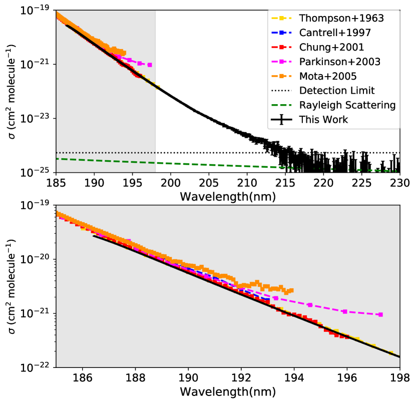
Figure 1: New H₂O absorption cross-sections compared to published data. Also plotted is the Rayleigh scattering cross-section, calculated as in Ranjan & Sasselov (2017). The top plot shows the full dataset; the bottom zooms in on the 185-198 nm wavelength region (highlighted in grey on the top plot) where data for comparison is available. The dotted black line demarcates the detection limit of our apparatus (Section 3.1).

3.2 Comparison to Previous Data & Theoretical Expectations

In this section, we compare our measurements (Figure 1) to previously published data and to theoretical expectations, to assess their quality and ascertain our confidence in them.

Data to compare our measurements to are nonexistent for $\lambda>198$ nm, but some datasets are available for $\lambda>190$ nm (Thompson et al., 1963; Cantrell et al., 1997; Chung et al., 2001; Parkinson & Yoshino, 2003; Mota et al., 2005). Our data agree with the measurements of Thompson et al. (1963), Cantrell et al. (1997), and Chung et al. (2001), with best agreement with the dataset of Chung et al. (2001), which is the most conservative of all datasets (i.e. presumes the lowest water absorption for wavelengths between 190 and 198 nm).

Our data agree with Mota et al. (2005) and Parkinson et al. (2003) at shorter wavelengths, but disagree with these datasets at their red edges. At these red edges, both Mota et al. (2005) and Parkinson et al. (2003) show distinctive upturns in the water absorption at the long-wavelength edge of their measurements, in disagreement with both the expected behavior of the spectra, and Chung et al. (2001) and Thompson et al. (1963). There are many possible explanations for such disagreement between sets of data, including experimental limitations (i.e. most of the disagreements occur at the instrumental threshold of measurements), variation in baseline corrections, and other experimental set-up concerns (e.g., whether equilibrium conditions in the system have been established before measurements, potential for underestimating water concentration, and scattering from H₂O in their saturated measurements). Of these, experimental limitations are a particularly compelling explanation, since the disagreements with Mota et al. (2005) and Parkinson et al. (2003) occur where one would expect them to be a problem, i.e. where their H₂O cross-sections are weakest and their measurement setups are closest to their limits. We therefore attribute the upturn at the red edges of the datasets of Mota et al. (2005) and Parkinson et al. (2003) to experimental error; we below apply this same logic to our own dataset.

Theoretical predictions expect that, at room temperature, water absorbs very weakly at wavelengths $\geq$180nm, losing intensity with a roughly exponential trend until it reaches the H-OH bond dissociation energy near 240 nm. This can be considered a vapor equivalent of Urbach’s rule which predicts that, as an electronically excited band moves away from its peak, the absorption coefficient decreases approximately as an exponential of the transition frequency (Quickenden & Irvin, 1980).

As wavelengths increase towards dissociation, the populations of the energy levels participating in the transitions that cause the spectral absorption become increasingly sparse. This thermal occupancy factor is the strongest effect in predicting absorption in this region, and corresponds to an exponential decay of transition strength, which gives the cross-section its recognizable log-linear shape between 180 and 240 nm. The opacity in this region is caused by transitions to excited electronic states of water, which are effectively unbound even at their lowest energy. Consequently, other weak effects can provide minor contributions towards the total absorption that can lead to a small upturn in the overall spectrum. For example, pre-dissociation effects can broaden the wings of the hot, combination rovibronic bands in the region, resulting in a small gain in opacity. Additionally, Frank-Condon factors and Einstein-A coefficients, which are hard to predict in this region, can increase near dissociation and consequently limit the loss of line strength caused by the reduction in thermal occupancy of the transition states.

The new measured data presented here agrees with the qualitative theoretical expectations of the spectral behaviour of water in the wavelength range 186 - 215 nm. From 215 nm to 230 nm, our measured data exhibit an upward deviation from log-linear decrease, similar to the deviation reported in the long-wavelength edge of other previously measured data (e.g., Parkinson et al. 2003; Mota et al. 2005). This upward deviation in all three datasets corresponds to the region of the measurements that approaches the instrumental noise floor, which not only introduces uncertainty to each measured data point, but also to the overall predicted absorption. It is therefore not fully certain that this upward deviation is physical.

Given the sensitivity of photochemical models to increased water absorption in the 186-230 nm region, we have adapted the measured cross-sections presented here to minimize the possibility that our predicted water absorption is overestimated. To this end, we considered two prescriptions for $292$K H₂O(g) absorption cross-sections for incorporation into our photochemical models. The first prescription corresponds to our measured data with a cut-off after 216.328 nm, which is where the ratio of the measured absorption to the errors first goes below 3. We term this the “cutoff” prescription. We note this is a conservative but unphysical prescription, since the water absorption at wavelengths above 216 nm is not expected to collapse, but instead experience an exponential loss in intensity. Our second data set addresses the concerns above by replacing the measured data at wavelengths $>$205 nm with a theoretical extrapolation, corresponding to a log-linear loss of absorption of our data from 186-205 nm towards dissociation (longer wavelengths). We term this the “extrapolation” prescription. This prescription is similar in spirit to that executed by Kasting & Walker (1981), but with the advantage of the greater spectral coverage and higher sensitivity of our new dataset, which significantly affect the results. We note that this extrapolation is expected to underestimate overall opacity (see above for potential quantum chemical effects that can increase opacity near dissociation).

Figure 2 presents both of our prescriptions for 292K NUV H₂O(g) absorption cross-sections; also shown are the prescription of Kasting & Walker (1981) and the recommended cross-sections of Sander et al. (2011). At wavelengths $<192$ nm, we employ the recommended cross-sections of Sander et al. (2011) (i.e. we replace the Parkinson et al. 2003 cross-sections of Sander et al. 2011). Both prescriptions specified here should be considered conservative choices, in that if anything they underestimate H₂O(g) absorption in this wavelength range. Nevertheless, both prescriptions indicate H₂O(g) absorption $\geq 205$ nm to be orders of magnitude higher than previously considered, with profound photochemical implications (Section 5). Both prescriptions, together with the underlying measurements, are available at https://github.com/sukritranjan/ranjanschwietermanharman2020.

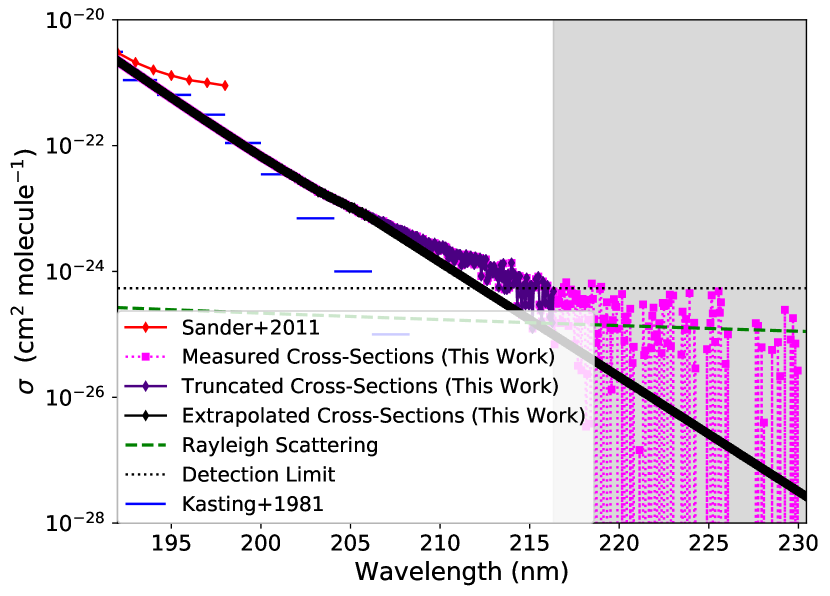
Figure 2: Cutoff and extrapolation prescriptions for the spectral absorption cross-sections of 292K H₂O(g). Also shown are the recommended cross-sections of Sander et al. (2011), the prescription of Kasting & Walker (1981), the Rayleigh scattering cross-sections (Ranjan & Sasselov, 2017), and the full dataset of measured cross-sections reported here. Our measured cross-sections first dip below a $3-\sigma$ significance at 216.348 nm; in the spirit of conservatism we consider our data at $>216.348$ nm unreliable, and demarcate it as such with grey shading. The dotted black line demarcates the detection limit of our apparatus (Section 3.1).

4 Model Intercomparison

We seek to determine the photochemical effects of our new H₂O cross-sections on the atmospheric composition of abiotic habitable worlds with anoxic CO₂-N₂ atmospheres. However, modelling of these atmospheres is discordant, with disagreement on a broad range of topics. Broadly, the models feature order-of-magnitude disagreements as to the trace gas composition of such atmospheres, and in particular their potential to accumulate photochemical CO and O₂ (Kasting, 1990; Zahnle et al., 2008; Hu et al., 2012; Tian et al., 2014; Domagal-Goldman et al., 2014; Harman et al., 2015; Rimmer & Helling, 2016; James & Hu, 2018; Hu et al., 2020).

To resolve this disagreement and derive a robust model for use in this work, we intercompare the models of Hu et al. (2012), Harman et al. (2015), and ATMOS (Arney et al. 2016, commit #be0de64; Archaean+haze template). For convenience, we allude to the model of Hu et al. (2012) as the “Hu model” and the model of Harman et al. (2015) as the “Kasting model” to reflect their primary developers, with the caveat that multiple workers have contributed to these models. We apply these models to the CO₂-dominated benchmark planetary scenario outlined in Hu et al. (2012). This scenario corresponds to an abiotic rocky planet orbiting a Sun-like star, with a 1-bar 90% CO₂, 10% N₂ atmosphere with surface temperature 288 K. Appendices A and  B present the details of the planetary scenario and boundary conditions adopted by these models. We focus on the surface mixing ratio of CO, $r_{CO}$, as the figure of merit for the intercomparison. At the outset of the intercomparison, the predictions of [CO] for this planetary scenario varied by $50\times$ between these models (Table 8).

We describe in detail the key differences between our models which drove the disagreement in $r_{CO}$ in Appendix C. Briefly, we identified the following errors and necessary corrections in our models (c.f. Appendix C, Table 4):

• Correction of CO₂ Absorption Cross-Sections: The Hu model approximated the NUV absorption cross-sections of CO₂ by its total extinction cross-sections out to 270 nm. However, measurements indicate that for $>201.58$ nm CO₂, extinction is scattering-dominated (Ityaksov et al. 2008) even though the reported bond dissociation energy of $532.2\pm 0.4$ kJ mol${}^{-}1$ (Darwent, 1970) corresponds to 225 nm. In high-CO₂ scenarios, this error shielded H₂O from NUV photolysis, regardless of assumptions regarding H₂O NUV absorption. This lead to underestimates of H₂O photolysis rates and [OH], and hence overestimates of [CO], [O], and [O₂]. We corrected the CO₂ cross-sections in the Hu model to correspond to absorption (Ityaksov et al., 2008; Keller-Rudek et al., 2013).

• Correction of Reaction Networks: We identified several errors in the reaction networks of the ATMOS and Kasting models. In the ATMOS model, these errors lead SO₂ to suppress CO, so that $r_{CO}$ was low regardless of assumptions on NUV H₂O absorption. In the Kasting model, these errors did not affect the baseline scenario, but lead to SO₂ suppression of CO in low-outgassing planetary scenarios. These errors and their suggested corrections are summarized in Appendix C, Table 5.

• Self-Consistent Temperature-Pressure Profile: The temperature-pressure profile in the ATMOS Archaean+haze scenario features a warm stratosphere, due to shortwave stratospheric heating from high-altitude haze ultimately sourced from high biogenic CH₄ emission. This leads to wet stratosphere and high H₂O photolysis rates. However, on a world lacking vigorous CH₄ production (e.g., an abiotic world), [CH₄] is low, haze is not expected to form, and CO₂-rich anoxic atmospheres are expected to have had cold, dry stratospheres (DeWitt et al., 2009; Guzmán-Marmolejo et al., 2013; Arney et al., 2016). Therefore, when employing ATMOS Archaean+haze to this planet scenario, it is necessary to first calculate a consistent temperature-pressure profile.

We identified the following points of difference between our models:

• Binary Diffusion Coefficient $nD(X,Y)$: Use of a generalized formulation (Equation C3) to estimate $nD(X,Y)$, relevant to diffusion-limited atmospheric escape, overestimates $nD(H_{2},N_{2})$ and $nD(H_{2},CO_{2})$ relative to laboratory measurements (Banks & Kockart, 1973; Marrero & Mason, 1972), and hence underestimates pH₂ and $r_{CO}$. Surprisingly, $nD(H,CO_{2})$ has not yet been measured; we recommend this as a target for future laboratory studies.

• $CO+OH$ Rate Law: Prescriptions for the rate constant of the reaction $CO+OH\rightarrow CO_{2}+H$ have evolved significantly. Moving forward, we recommend the prescription of Burkholder et al. (2015), which is the most up-to-date known, and is intermediate relative to the prescriptions incorporated into our models to date.

• $CO+S+M$ Rate Law: The reaction $CO+S+M\rightarrow OCS+M$ has not been measured in the laboratory, but has been invoked to explain Venusian OCS (Krasnopolsky, 2007; Yung et al., 2009). Assumption of this reaction modestly reduces $r_{CO}$. We identify this as a key reaction for laboratory follow-up; confirmation of this reaction mechanism will affirm our understanding of Venusian atmospheric chemistry, while refutation will signal a need to closely re-examine our photochemical models of Venus and Venusian exoplanets.

If we repair these errors and align these parameters between our models, we find that our model predictions of $r_{CO}$ agree to within a factor of $2$, and that we can reproduce both the low ($\sim$200 ppm) and high ($\sim 8200$ ppm) estimates for $r_{CO}$ that have been reported in the literature (Section C.5; Appendix C, Table 6). The overwhelmingly dominant factor is the prescription adopted for the NUV absorption cross-sections of H₂O(g). Prescriptions that omit this absorption (e.g., Sander et al. 2011) lead to high $r_{CO}$, and prescriptions that include this absorption (e.g., Kasting & Walker 1981) lead to low $r_{CO}$. The absorption measured in this work is higher in the NUV than considered by any of these prescriptions (Figure 2), implying $r_{CO}$ to be lower than previously calculated by any model (Section 5). We conclude that we have resolved the disagreements between our models as measured by predictions of $r_{CO}$.

5 Updated Photochemical Model

We include our newly measured H₂O cross-sections in the corrected Hu model, using both the extrapolated and cutoff prescriptions detailed in Section 3.2. We verify that the model still reproduces the atmospheres of modern Earth and modern Mars as detailed in Hu et al. (2012). Table 1 presents the effects of the new H₂O cross-sections on $r_{CO}$ and $r_{O_{2}}$ for the CO₂-dominated exoplanet scenario of Hu et al. (2012). For these calculations, we returned to the simulation parameters as originally prescribed by Hu et al. (2012), following the rationale given therein and to facilitate comparison with past results. In other words, we followed the simulation parameters tabulated in Table 2, not the uniform parameters adopted for the model intercomparison in Appendix C.5. For all model runs, we verified maintenance of atmospheric redox balance (Hu et al., 2012).

Table 1: Summary of results from corrected model (i.e. with corrected CO₂ cross-sections), with results from uncorrected model also shown for context. The first sub-table, titled “Standard Scenario”, illustrates the effect of different prescriptions for H₂O NUV absorption on CO and O₂ concentrations in our standard scenario (Table 3). The second sub-table, titled “Reduced Outgassing Scenarios”, illustrates the effect of our new cross-sections on the abiotic O₂ buildup scenario reported in Hu et al. (2012). The enhanced H₂O photolysis efficiently recombines CO and O₂, and removes this abiotic false-positive scenario for O₂. In this table, $r_{X}$ is the surface mixing ratio of $X$ (relative to dry CO₂+N₂). $J_{H_{2}O}$ is the column-integrated photolysis rate. $\Phi_{Dep}$ is the net flux of reducing power out of the ocean, in H-equivalents, relevant to the question of global redox balance ($\Phi_{Dep}<0\Rightarrow$ reducing power enters the ocean).

Parameters	$r_{CO}$	$r_{O_{2}}$	$J_{H_{2}O}$	$\Phi_{Dep}$
			(cm-2 s-1)	(H cm-2 s-1)
Standard Scenario
Uncorrected model	8.2E-3	1.5E-14	1.0E8	-4.2E9
Sander et al. (2011) H2O	6.4E-3	9.2E-19	9.3E7	-3.7E9
Kasting & Walker (1981) H2O	1.2E-4	9.5E-19	1.2E10	-2.0E10
Cutoff H2O (this work)	8.6E-6	7.2E-12	6.6E10	-6.0E10
Extrapolated H2O (this work)	1.3E-5	2.5E-12	5.3E10	-5.8E10
Reduced Outgassing Scenarios
$\phi_{H_{2}}=3\times 10^{9}$ cm-2 s-1
Uncorrected model	1.2E-2	3.2E-6	3.0E7	-4.3E9
Sander et al. (2011) H2O	9.5E-3	3.0E-6	2.9E7	-3.7E9
Extrapolated H2O (this work)	1.5E-5	2.8E-11	5.3E10	-8.5E9
$\phi_{H_{2}}=\phi_{CH_{4}}=0$ cm-2 s-1
Uncorrected model	3.7E-2	1.5E-3	9.1E6	-1.8E9
Sander et al. (2011) H2O	1.6E-2	2.1E-4	9.8E6	-1.8E9
Extrapolated H2O (this work)	1.6E-5	3.4E-11	5.3E10	-4.8E8

5.1 Effect of New Cross-Sections on $r_{CO}$ and $r_{O_{2}}$

The effects are dramatic: inclusion of the new H₂O cross-sections, whether using the extrapolated or cutoff prescriptions, reduces $r_{CO}$ by 2.5 orders of magnitude relative to the cross-sections recommended by Sander et al. (2011) (i.e., terminated at 198 nm), and 1 order of magnitude relative to the Kasting & Walker (1981) prescription, to $\sim 10$ ppm (Figure 3), for our abiotic CO₂-N₂ scenario. The new H₂O cross-sections are larger and extend to longer wavelengths than the prescription of Kasting & Walker (1981), leading to H₂O photolysis rates that are $\sim 5$ times higher. These higher photolysis rates drive enhanced production of OH, especially at the bottom of the atmosphere where [H₂O] is highest (Figure 4), resulting in the efficient recombination of CO and O to CO₂ via catalytic cycles ultimately triggered by $CO+OH\rightarrow CO_{2}+H$ (Harman et al., 2018). The new cross-sections also drive enhanced production of H, visible as enhanced [H] in the bottom of the atmosphere.

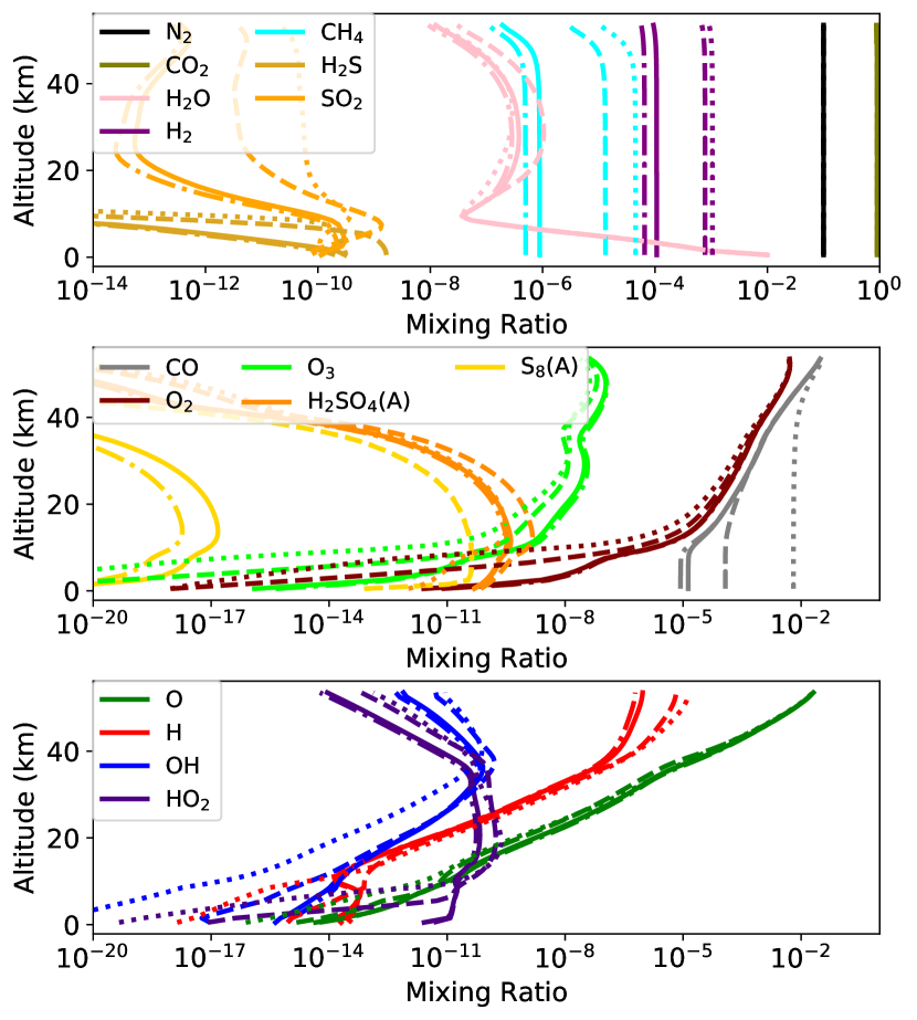
Figure 3: Mixing ratio (relative to dry CO₂/N₂) as a function of altitude for outgassed species (top), photochemical byproducts (middle), and radicals (bottom). These predictions were derived from the Hu model, with corrected CO₂ cross-sections. The line types demarcate different prescriptions regarding the H₂O cross-sections. Specifically, the solid lines refer to the “extrapolation” prescription proposed here; the dash-dotted lines, the “cutoff” prescription; the dashed lines, the Kasting & Walker (1981) prescription; and the dotted lines, the Sander et al. (2011) prescription. The higher H₂O absorption we propose here leads to higher [OH] and [H], and concommitantly lower [CO], [CH₄], and [H₂].

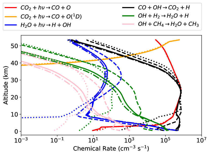
Figure 4: Key reaction rates as a function of altitude. These predictions were derived from the Hu model, with corrected CO₂ cross-sections. The line types demarcate different prescriptions regarding the H₂O cross-sections. Specifically, the solid lines refer to the “extrapolation” prescription proposed here; the dash-dotted lines, the “cutoff” prescription; the dashed lines, the Kasting & Walker (1981) prescription; and the dotted lines, the Sander et al. (2011) prescription. The higher H₂O absorption we propose here dramatically enhances OH and H production from H₂O photolysis, especially in the bottom of the atmosphere, leading to much lower CO, CH₄, and H₂ due to suppression by OH.

Our H₂O absorption cross-sections also negate the low-outgassing photochemical false positive scenario for O₂ on planets orbiting Sun-like stars. Specifically, it has been proposed that in the regime of lower outgassing of reductants (H₂, CH₄), O₂ sourced from CO₂ photolysis can accumulate to detectable, near-biotic levels on planets orbiting solar-type stars. This constitutes a potential false positive scenario for O₂ as a biosignature gas (Hu et al., 2012; Harman et al., 2015; James & Hu, 2018). With our new H₂O cross-sections, we find photolytic OH efficiently recombines CO and O even in the absence of CH₄ and H₂ outgassing (Figure 5). Interestingly, though we find very low H₂ and CH₄ in the low-outgassing case, we nonetheless report higher pH₂ and pCH₄ compared to Hu et al. (2012). We speculate H sourced from H₂O photolysis to support the CH₄ and H₂.

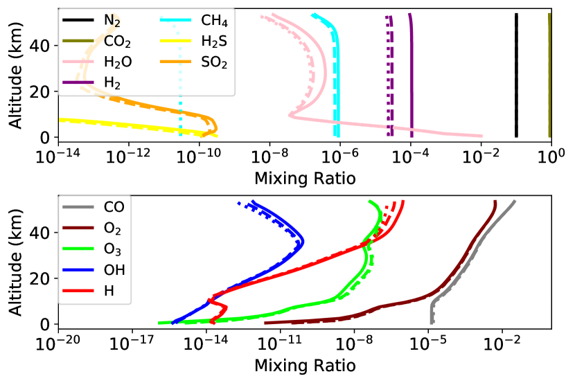
Figure 5: Mixing ratio (relative to dry CO₂/N₂) as a function of altitude for outgassed species (top) and photochemical byproducts (bottom), calculated with the corrected Hu model and with the extrapolation prescription for H₂O absorption. The solid lines assume full outgassing ($\phi_{H_{2}}=3\times 10^{10}$ cm^-2 s^-1, $\phi_{CH_{4}}=3\times 10^{8}$ cm^-2 s^-1); the dashed lines, reduced outgassing ($\phi_{H_{2}}=3\times 10^{9}$ cm^-2 s^-1, $\phi_{CH_{4}}=3\times 10^{8}$ cm^-2 s^-1); and the dotted lines no outgassing of H₂ and CH₄ ($\phi_{H_{2}}=0$ cm^-2 s^-1. The higher H₂O absorption we measure obviates the low-outgassing false photochemical false positive mechanism for O₂.

5.2 Effect of New Cross-Sections on Other Atmospheric Gases

OH is a powerful oxidizing agent, and efficiently reacts with a broad range of reduced species (e.g., Catling & Kasting 2017). It is consequently unsurprising to find that the enhancement in OH production from our larger H₂O cross-sections leads to suppression of a broad range of the trace compounds present in anoxic atmospheres, including H₂S, SO₂, and S₈ aerosol (Figure 3)

Perhaps most dramatic is the suppression of CH₄. With our new H₂O cross-sections, we predict the concentration of volcanically-outgassed CH₄ to be 2 orders of magnitude lower than using the Sander et al. (2011) cross-sections and 1.5 orders of magnitude lower than using the Kasting & Walker (1981) cross-sections. We predict the main sink on CH₄ to be OH via the reaction $OH+CH_{4}\rightarrow CH_{3}+H_{2}O$, consistent with previous work (e.g., Rugheimer & Kaltenegger 2018). This suppression of CH₄ is significant because CH₄ is spectrally active, and has been proposed as a potentially detectable component of exoplanet atmospheres and a probe of planetary processes, including life (Guzmán-Marmolejo et al., 2013; Rugheimer & Kaltenegger, 2018; Krissansen-Totton et al., 2018). Our work suggests it may be harder to detect this gas in anoxic atmospheres than previously considered.

Also key is our finding of photochemical suppression of H₂ (but see caveat below). Prior simulations concluded that the main sink on H₂ on anoxic terrestrial planets (e.g. early Earth) was escape to space and that pH₂ was to first order set by the balance between H₂ outgassing and (diffusion-limited) escape (Kasting, 1993, 2014). Indeed, under the assumption of the Kasting & Walker (1981) cross-sections, we recover this result ourselves. However, with our new cross-sections, we find the sink due to the reaction $H_{2}+OH\rightarrow H_{2}O+H$ to be the dominant sink on H₂, which suppresses p$H_{2}$ by 1 order of magnitude relative to past predictions. This reaction converts relatively unreactive H₂ to relatively reactive H, which can undergo further reactions to ultimately be deposited to the surface in the form of more-soluble reduced chemical species. This is reflected in enhanced transfer of reductants from the atmosphere to the oceans calculated by our model (Table 1), in which essentially all of the reducing power outgassed as H₂ is returned to the surface, primarily via rainout. This suggests more efficient delivery of reduced organic compounds from the atmosphere, of relevance to origin-of-life studies (e.g., Cleaves 2008; Harman et al. 2013; Rimmer & Rugheimer 2019).

The above results were derived without assuming global redox balance (Kasting, 2013; Tian et al., 2014; Harman et al., 2015; James & Hu, 2018). The principle of global redox balance is based on the observation that the main mechanisms by which we know free electrons to be added or removed from the ocean-atmosphere system on Earth are oxidative weathering and biologically-mediated burial of reductants. The former is not relevant to anoxic atmospheres; the latter is not relevant to abiotic worlds. If one zeroes these terms in the atmosphere-ocean redox budgets, one finds that in steady-state, any supply of reductants or oxidants to the planet surface should be counterbalanced by return flux to or deposition from the atmosphere (Harman et al., 2015). This is practically implemented in models by prescribing an oceanic H₂ return flux in the case where reductants are net deposited into the ocean by the atmosphere (mostly by rainout), or an increased H₂ deposition velocity in the (uncommon) case where oxidants are net deposited (Tian et al., 2014; Harman et al., 2015; James & Hu, 2018). Figure 6 presents the effects of requiring global redox balance. We find a return flux of $4.4\times 10^{10}$ cm^-2 s^-1, a return of pH₂ to the escape-limited $1\times 10^{-3}$ bar, and an increase in CH₄ by 1 order of magnitude ($2\times$ lower than when assuming the Kasting & Walker 1981 cross-sections). Overall, we predict pH₂ and pCH₄ to be significantly an order-of-magnitude higher on worlds obeying global redox balance, as has been proposed for abiotic worlds.

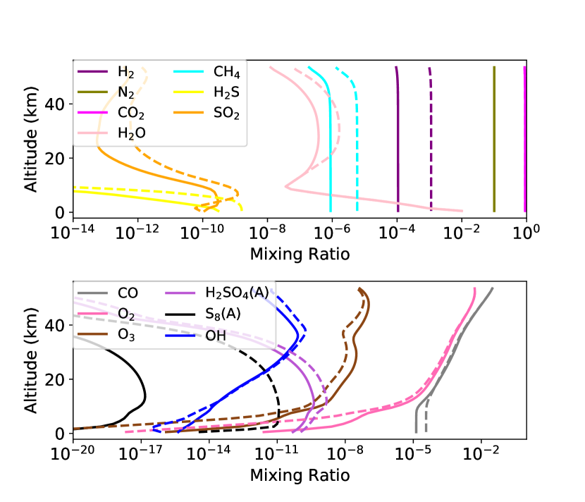
Figure 6: Mixing ratio (relative to dry CO₂/N₂) as a function of altitude for outgassed species (top) and photochemical byproducts (bottom), calculated with the corrected Hu model and with the extrapolation prescription for H₂O absorption. The solid lines were calculated without assuming global redox balance; the dashed lines assumed global redox balance. Redox balance makes the atmosphere more reducing, stabilizing reduced species.

Our calculations highlight the importance of the question of global redox balance for abiotic planets. In the past, it has been possible to largely ignore this question in conventional planetary scenarios, because the deposition terms in the redox budget have been relatively small. However, our new cross-sections suggest that the processing of H₂ into soluble reductants is efficient, the deposition terms are large, and the assumption of global redox balance has significant impact on the buildup of spectrally-active, potentially-detectable species in conventional planetary scenarios.

Whether abiotic anoxic planets are in global redox balance requires careful consideration. The theory of global redox balance rests on the assumption that biological mediation is required for burial of reductants. Biologically-mediated burial is the dominant mode on modern Earth (Walker, 1974). However, to our knowledge it is not yet determined whether biotic burial is the only possible mode of reductant burial. We may draw an analogy to the theory of abiotic nitrogen fixation, where it was long assumed that on abiotic worlds (e.g, prebiotic Earth), lightning-fixed nitrogen could accumulate almost indefinitely in the ocean as nitrate/nitrite (NO${}_{X}^{-}$), since the today-dominant biological sinks of NO${}_{X}^{-}$ were absent (e.g., Mancinelli & McKay 1988; Wong et al. 2017; Hu & Diaz 2019). However, there exist abiotic sinks on NO${}_{X}^{-}$, slower than the biotic sinks but still important on geological timescales; these sinks suppress oceanic [NO${}_{X}^{-}$] and stabilize atmospheric N₂ (Ranjan et al., 2019). Similarly, there may exist abiotic reductant/oxidant burial mechanisms which are relevant on geological timescales (e.g., Fe²⁺ photooxidation, Kasting et al. 1984; magnetite burial, James & Hu 2018); the existence of such mechanisms should be explored further. Alternately, Mars may provide a touchstone. Like Earth, early Mars should have hosted an abiotic ocean under an anoxic atmosphere, but unlike Earth, the lack of tectonic activity and hydrology means that geological evidence from this epoch may be preserved (Citron et al., 2018; Sasselov et al., 2020). Are there geological fingerprints of the presence or absence of redox balance (e.g, evidence of widespread abiotic reductant burial) that future missions might detect? If so, such measurements could bound the relevant parameter space for the global redox balance hypothesis.

6 Discussion & Conclusions

We present the first measurements of H₂O cross-sections in the NUV ($>200$ nm) at habitable temperatures ($T=292~{}\text{K}<373$ K), and show them to be far higher than assumed by previous prescriptions. These cross-sections are critical because in anoxic atmospheres the atmosphere is transparent at these wavelengths, and water can efficiently photolyze down to the surface (Harman et al., 2015; Ranjan & Sasselov, 2017). In anoxic atmospheres, this H₂O photolysis is the ultimate source of atmospheric OH, a key control on atmospheric chemistry in general and CO in particular.

To assess the photochemical impact of these new cross-sections on atmospheric composition, we apply a photochemical model to a planetary scenario corresponding to an abiotic habitable planet with an anoxic, CO₂-N₂ atmosphere orbiting a Sunlike star. This planet scenario is representative of early (prebiotic) Earth, Mars and Venus, and analogous exoplanets. Model predictions of the atmospheric composition of such worlds are highly divergent in the literature; through a model intercomparison, we have identified the errors and divergent assumptions driving these differences, and reconciled our models.

Incorporating these newly-measured cross-sections into our corrected model enhances OH production and suppresses $r_{CO}$ by $1-2.5$ orders of magnitude relative to past calculations. This implies less CO on early Earth for prebiotic chemistry and primitive ecosystems (Kasting, 2014), suggesting the need to consider alternate reductants. It also implies that CO will be a more challenging observational target for rocky exoplanet observations that we might previously have hoped. However, if surface production of CO from processes like impacts, volcanism or biology (Kasting, 2014; Schwieterman et al., 2019; Wogan & Catling, 2020) is sufficient to saturate the enhanced OH sink due to more efficient H₂O photolysis, CO may yet enter runaway and build to potentially-detectable concentrations; we plan further investigation. On the other hand, the more efficient OH-catalyzed recombination of CO and O also removes the proposed low-outgassing false-positive mechanism for O₂ (Hu et al., 2012). This reduces (but does not completely obviate; Wordsworth & Pierrehumbert 2014) the potential ambiguities regarding O₂ as a biosignature for planets orbiting Sunlike stars.

The situation on planets orbiting lower-mass stars, e.g. M-dwarfs, may be different. These cooler stars are dimmer in the NUV compared to Sunlike stars, meaning we expect the effect of our enhanced NUV H₂O cross-sections to be muted (Segura et al., 2005; Ranjan et al., 2017). On these planets, higher $r_{CO}$ and $r_{O_{2}}$ may be possible (Schwieterman et al., 2019; Hu et al., 2020); we plan further study. Further, these results do not impact O₂-rich planets analogous to the modern Earth, since in these atmospheres direct H₂O photolysis is a minor contributor to OH production.

In addition to CO, H₂O-derived OH can suppress a broad range of species in anoxic atmospheres. In particular, the larger H₂O cross-sections we measure in this work lead to substantial enhancements in OH attack on H₂ and CH₄, suppressing these gases in the abiotic scenario by 1-2 orders of magnitude relative to past calculations, and suggesting that spectroscopic detection of CH₄ on anoxic exoplanets will be substantially more challenging than previously considered (Reinhard et al., 2017; Krissansen-Totton et al., 2018). However, this finding is sensitive to assumption of global redox balance. If reductants cannot be removed from the ocean by burial, as has been proposed for abiotic planets, then the return flux of reductants from the ocean (parametrized as H₂) compensates for much of the CH₄ and all of the H₂ suppression. Regardless, rainout of reductants to the surface is enhanced, relevant to prebiotic chemistry (c.f. Benner et al. 2019)

In prior calculations, enforcement of global redox balance resulted in relatively small changes in many planetary scenarios, including the scenario studied here. With the enhanced OH production driven by our higher H₂O cross-sections, this is no longer the case. This highlights the need to carefully consider global redox balance, and in particular its key premise that abiotic reductant burial is always geologically insignificant. Early Mars may provide a test case for the theory of redox balance, in that it may have hosted an abiotic ocean underlying an anoxic atmosphere early in its history, and geological remnants of this era might persist due to the lack of hydrologic and tectonic activity since 3.5 Ga. If abiotic reductant burial produce a detectable geological signature, then future missions can search for that signature, directly testing the global redox balance hypothesis. Further work, to consider processes and signatures of abiotic reductant burial, is required.

In this paper, we have focused on an abiotic planet scenario. We note that all of our specific findings (e.g., very low $r_{CO}$) may not generalize to biotic scenarios. Biological production or uptake of gases may significantly outpace photochemical sources and sinks; for example, if biological CO production can outpace photolytic OH supply, then CO may nonetheless build to high, potentially-detectable concentrations (Schwieterman et al., 2019). Detailed case-by-case modelling of biotic scenarios is required. However, our general point that OH production is higher than previously considered on anoxic habitable planets applies to biotic worlds as well, implying that spectrally active trace gases have a higher bar to clear to build to high concentrations than previously considered.

In this work, we have ignored nitrogenous chemistry, in particular the NO_X catalytic chemistry triggered by lightning-generated NO (Ardaseva et al., 2017; Harman et al., 2018). We justify this exclusion on the basis that this chemistry is most important when CO is high (Kasting, 1990), and our models indicate that CO is photochemically suppressed. We conducted a sensitivity test to the inclusion of NO-triggered nitrogenous chemistry with the Kasting model, and found negligible (percent-level) impact on $r_{CO}$. Note that nitrogenous chemistry has been proposed to play a more dominant role on M-dwarf planets (Hu et al., 2020); for such worlds, this chemistry must be included.

Our work highlights the critical need for laboratory measurements and/or theoretical calculations of the inputs to photochemical models. We show the sensitivity of the models to H₂O NUV cross-sections; we recommend further characterization of these cross-sections, both to confirm our own results and to extend these cross-sections, e.g. to longer wavelengths and lower temperatures. In particular, we reiterate that our prescriptions for H₂O NUV cross-sections are conservative, and the true absorption may be yet higher; higher signal-to-noise measurements at longer wavelengths are required to rule on this possibility. Further, our 292K cross-sections are good proxies for H₂O absorption on temperate terrestrial planets, because the nonlinear decrease in H₂O saturation pressure with temperature means that most H₂O is confined to the temperate lower atmosphere. However, on cold planets (e.g., modern Mars), the lower atmosphere is also cold, meaning use of 292K cross-sections may overestimate the H₂O opacity and photolysis rate. Similarly, we have here assumed a photolysis quantum efficiency of unity, i.e. that absorption of each $\leq 230$ nm photon leads to H₂O photolysis. If this assumption is incorrect, then the true photolysis rate will be lower than we have modelled here.

Finally, some of the reactions encoded into our models and/or their reaction rate constants are assumed or disputed; these reactions should be experimentally or theoretically characterized, to confirm or refute these assumptions. In particular, we identify the reactions $CO+S+M\rightarrow OCS+M$, $HO_{2}+SO_{2}\rightarrow OH+SO_{3}$, $HO_{2}+SO_{2}\rightarrow O_{2}+HSO_{2}$, $SO+HO_{2}\rightarrow SO_{2}+OH$, $SO+HO_{2}\rightarrow SO_{2}+OH$, $SO+HO_{2}\rightarrow O_{2}+HSO$, and $N+O_{3}\rightarrow NO+O_{2}$ as targets for further investigation (Graham et al., 1979; Yung & Demore, 1982; Wang & Hou, 2005; Yung et al., 2009; Burkholder et al., 2015).

Appendix A Detailed Simulation Parameters for Planetary Scenario

In Table 2, we present the simulation parameters of our models for the CO₂-dominated planet scenario we consider. To make our models agree, we must implement the corrections summarized in Table 4, and adjusting our models to use common inputs and formalisms as summarized in Table 7.

Table 2: Simulation Parameters For Planetary Scenario.

Scenario Parameter	Hu	ATMOS	Kasting
Model	Hu et al. (2012)	Arney et al. (2016)	Harman et al. (2015)
Reaction Network	As in Hu et al. (2012)	Archean Scenario	As in Harman et al. (2015)
	(Excludes N-, C>2-chem)
Stellar type	Sun	Sun	Sun
Semi-major axis		1.3 AU
Planet size		1 M⊕, 1 R⊕
Surface albedo	0.	0.25	0.25
Major atmospheric components		0.9 bar CO2, 0.1 bar N${}_{2}^{\star}$
Surface temperature ($z=0$ km)		288K
Surface $r_{H_{2}O}$ (lowest atmospheric bin)		0.01
Eddy Diffusion Profile		See Figure 9
Temperature-Pressure Profile		See Figure 9
Vertical Resolution	0-54 km, 1 km steps	0-100 km, 0.5 km steps	0-100 km, 1 km steps
Rainout	Earthlike; rainout turned off for	Earthlike (all species)	Earthlike (all species)
	H2, CO, CH4, NH3, N2, C2H2,
	C2H4, C2H6, and O2 to simulate
	saturated ocean on abiotic planet
Lightning		Off
Global Redox Conservation	No	No	Yes

Note. — ^⋆In Hu model, pN₂ is fixed. In the ATMOS and Kasting models, pN₂ is adjusted to maintain dry $P=1$ bar. Photochemical and outgassed products do not build to levels comparable to the N₂ inventory in the scenario simulated here, and consequently this difference does not affect our results

Appendix B Detailed Boundary Conditions for Planetary Scenario

In this Appendix, we present the species used in each of our models and their corresponding boundary conditions used in our initial model reconciliation. For all species, we assign either a fixed surface mixing ratio or a surface flux. CO₂, N₂, and H₂O are the only species assigned fixed surface mixing ratios (for rationale, see Hu et al. 2012). For species with a surface flux, the species is assumed to be injected in the bottommost layer of the atmosphere, i.e. PARAMNAME=1 in ATMOS. H and H₂ are assumed to escape at their diffusion-limited rates; for all other species, the escape/delivery flux is prescribed as 0.

While our models generally assume the same major species and many of the same minor species, there are some key differences, driven primarily by different assumptions regarding reaction network. In particular:

1. The Kasting model does not include polysulfur species. This is because the polymerization of elemental sulfur to form S₈ aerosol is ignored, on the basis that this is a minor exit for S in this relatively oxidized atmospheric scenario; instead, S is assigned a high deposition velocity of 1 cm s^-1.

2. The Hu model excludes all nitrogenous species other than N₂. This is because the chosen boundary conditions precluded reactive N (no lightning, no thermospheric N), meaning they could neglect N-chemistry.

In the planetary scenario considered here, these differences do not significantly affect $r_{CO}$, and we ignore them for purposes of this model intercomparison.

Table 3: Species choice and treatment for the photochemical models used in this study.

Species		Type		Surface Flux	Surface Mixing Ratio	Dry Deposition Velocity	TOA Flux
	Hu	ATMOS	Kasting	(cm-2 s-1)	(relative to CO2+N2)	(cm s-1)	(cm-2 s-1)
H	X	X	X	0	–	1	Diffusion-limited
H2	X	X	X	$3\times 10^{10}$	–	0	Diffusion-limited
O	X	X	X	0	–	1	0
O(1D)	X	F	F	0	–	0	0
O2	X	X	X	0	–	0	0
O3	X	X	F	0	–	0.4	0
OH	X	X	X	0	–	1	0
HO2	X	X	X	0	–	1	0
H2O	X	X	X	–	0.01	0	0
H2O2	X	X	X	0	–	0.5	0
CO2	X	C	X	–	0.9	0	0
CO	X	X	X	0	–	$1\times 10^{-8}$	0
CH2O	X	-	X	0	–	0.1	0
CHO	X	-	X	0	–	0.1	0
C	X	-	-	0	–	0	0
CH	X	X	-	0	–	0	0
CH2	X	-	-	0	–	0	0
1CH2	X	F	F	0	–	0	0
3CH2	X	X	F	0	–	0	0
CH3	X	X	X	0	–	0	0
CH4	X	X	X	$3\times 10^{8}$	–	0	0
CH3O	X	X	F	0	–	0.1	0
CH4O	X	-	-	0	–	0.1	0
CHO2	X	-	-	0	–	0.1	0
CH2O2	X	-	-	0	–	0.1	0
CH3O2	X	X	F	0	–	0	0
CH4O2	X	-	-	0	–	0.1	0
C2	X	X	-	0	–	0	0
C2H	X	X	-	0	–	0	0
C2H2	X	X	-	0	–	0	0
C2H3	X	X	-	0	–	0	0
C2H4	X	X	-	0	–	0	0
C2H5	X	X	F	0	–	0	0
C2H6	X	X	X	0	–	$1\times 10^{-5}$	0
C2HO	X	-	-	0	–	0	0
C2H2O	X	-	-	0	–	0.1	0
C2H3O	X	-	F	0	–	0.1	0
C2H4O	X	-	-	0	–	0.1	0
C2H5O	X	-	-	0	–	0.1	0
S	X	X	-	0	–	0	0
S2	X	X	-	0	–	0	0
S3	X	F	-	0	–	0	0
S4	X	F	-	0	–	0	0
SO	X	X	X	0	–	0	0
SO2	X	X	X	$3\times 10^{9}$	–	1	0
1SO2	X	F	F	0	–	0	0
3SO2	X	F	F	0	–	0	0
H2S	X	X	X	$3\times 10^{8}$	–	0.015	0
HS	X	X	X	0	–	0	0
HSO	X	X	X	0	–	0	0
HSO2	X	-	-	0	–	0	0
HSO3	X	F	F	0	–	0.1	0
HSO4	X	X	X	0	–	1	0
H2SO4(A)	A	A	A	0	–	0.2	0
S8	X	-	-	0	–	0	0
S8(A)	A	A	-	0	–	0.2	0
N2	C	C	C	–	0.1	0	0
OCS	X	X	-	0	–	0.01	0
CS	X	X	-	0	–	0.01	0
CH3S	X	-	-	0	–	0.01	0
CH4S	X	-	-	0	–	0.01	0

Note. — (1) For species type, for each model, “X” means the full continuity-diffusion equation is solved for the species; “F” means it is treated as being in photochemical equilibrium; “A” means it is an aerosol and falls out of the atmosphere; “C” means it is treated as chemically inert; and “–” means that it is not included in that model. Note that boundary conditions like dry deposition velocity are not relevant for Type “F” species, since transport is not included for such species. The exclusion of a species from a model does not necessarily mean that the model is incapable of simulating the species, but just that it was not included in the atmospheric scenario selected here. For example, following Hu et al. (2012), the Hu model was deployed here without N species because the planet scenario selected here precludes reactive N, though it is capable of simulating nitrogenous chemistry. (2) For the bottom boundary condition, either a surface flux is specified, or a surface mixing ratio. N₂ is a special case in the Kasting model and in ATMOS; in these models, [N₂] is adjusted to set the total dry pressure of the atmosphere to be 1 bar (to account for outgassed species and photochemical intermediates). Consequently, pN${}_{2}\lesssim 0.1$ bar in these models. (3) TOA flux refers to the magnitude of outflow at the top-of-the-atmosphere (TOA); hence, a negative number would correspond to an inflow.

Appendix C Detailed Model Intercomparison

In this Appendix, we enumerate the model differences which drove the divergent predictions of $r_{CO}$. Some of these differences were errors; we discuss them below, and summarize their correction in Table 4.

Table 4: Required Corrections To the Models

Model	Correction
Hu	Removal of erroneous $>202$ nm CO2 absorption (Section C.1).
ATMOS, Kasting	Correction of reaction network (Section C.2)
ATMOS	Use of self-consistent T-P-H2O Profile (Section C.3)

C.1 CO₂ and H₂O Cross-Sections

Our model intercomparison reveals the single strongest control on $r_{CO}$ to be treatment of the H₂O and CO₂ cross-sections. The abundance of CO in habitable planet atmospheres is photochemically controlled by a balance of CO₂ photolysis, which generates CO, and H₂O photolysis, which is the ultimate source of the OH radicals that recombine CO and O to CO₂ (c.f. Section 2). The Hu model incorrectly implemented CO₂ absorption. Specifically, Hu et al. (2012) approximated the absorption cross-sections by the total-extinction cross-sections from Ityaksov et al. (2008). However, at wavelengths $>201.58$ nm, the extinction cross-section is dominated by scattering, and the absorption is $\approx 0$. Therefore, this error led to unphysical absorption from CO₂ and suppression of the UV radiation field at $\geq 202$ nm. This suppression was particularly acute because of the high scattering optical depth at $\sim$200 nm in the CO₂-dominated atmosphere, which amplified the unphysical absorption due to CO₂ (Bohren, 1987; Ranjan et al., 2017). CO₂ absorption at $\geq 204$ nm was not assumed to lead to photolysis, so CO₂ photolysis itself was not overestimated due to this error.

Upon correction of the CO₂ absorption cross-sections, the atmosphere is largely transparent at wavelengths $\geq$ 202 nm except for H₂O. Prior to this work, no experimentally measured or theoretically predicted absorption cross-sections were available for H₂O(g) at $>198$ nm at conditions relevant to temperate rocky planets ($T\sim 300$ K) The cross-sections recommended by Burkholder et al. (2015), ultimately sourced from Parkinson et al. (2003), terminate at 198 nm due to lack of data. However, as originally pointed out by Kasting & Walker (1981), it is unphysical to assume that H₂O absorption should abruptly terminate at $\sim 200$ nm. The dissociation energy of the H-OH bond corresponds to photons of wavelength $\sim 240$ nm, and photolysis should continue down to that wavelength, albeit at steadily lower cross-section. Consequently, models descended from Kasting & Walker (1981), in this study ATMOS and Kasting, extrapolate the H₂O cross-sections from Thompson et al. (1963) out to longer wavelengths (Figure 2). This leads to H₂O photolysis and CO recombination at low altitudes (Harman et al., 2015). The Hu model originally used this extrapolation as well; however, due to the error in the CO₂ cross-sections, H₂O photolysis was suppressed at low altitudes, regardless of whether this extrapolation was included, and the Hu model eventually adopted the recommendation of Burkholder et al. (2015) for the H₂O cross-sections.

If either the erroneous longwave CO₂ absorption is present, or the H₂O absorption extrapolation is neglected, then H₂O photolysis is suppressed and $r_{CO}$ is high. CO₂ does not absorb $>202$ nm, and in Section 3 we experimentally demonstrate that H₂O does indeed absorb at such wavelengths. Indeed, it absorbs larger cross-sections than assumed by the ATMOS and Kasting models, meaning that H₂O photolysis, and hence CO recombination, is more intense than predicted by all three of the baseline models (Figure 2). Further, the latest data suggest CO₂ absorption terminates by 202 nm, shorter than all three of the models considered here, meaning that CO₂ photolysis (and hence CO production) is lower than assumed by all three of the models (Figure 7). Therefore, CO should not only be lower than predicted by the baseline Hu model, it should be lower than predicted by all three of our models (Section 5).

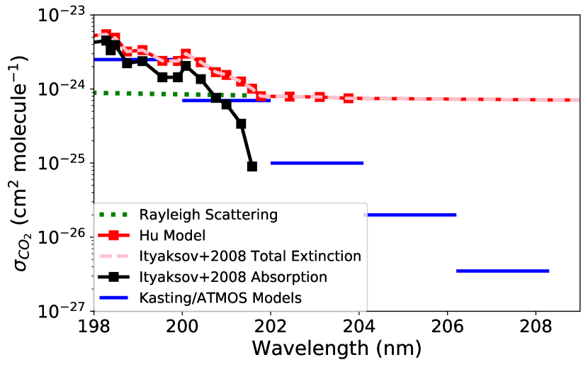
Figure 7: CO₂ absorption cross-sections assumed by Hu and ATMOS/Kasting models. The total extinction and absorption cross-sections from Ityaksov et al. (2008) are also shown for reference, as is the CO₂ Rayleigh scattering cross-section calculated as in Ranjan & Sasselov (2017).

C.2 Reaction Network

In our intercomparison, we found SO₂ outgassing to suppress $r_{CO}$ in ATMOS. SO₂ did not suppress $r_{CO}$ in the Kasting model in the baseline scenario, but did in the Kasting model in the low-outgassing regime (0 CH₄, H₂ outgassing; Hu et al. 2012). We intercompared the Hu, Kasting, and ATMOS reaction networks, with particular emphasis on the sulfur chemistry. We identified a number of discrepancies in the Kasting and ATMOS models, summarized in Table 5. The discrepancies in the Kasting models were incorrect implementations of published reactions or rates. The discrepancies in ATMOS were the deactivation of known reactions; the rationale for these deactivations is not known. The primary effect of the correction of these discrepancies is to remove the effect whereby SO₂ outgassing suppresses $r_{CO}$, in all regimes evaluated in this study.

Table 5: Required updates to reaction networks

Reaction	Old Parameter	Corrected Parameter	Reference
Kasting	$\cdots$	$\cdots$	$\cdots$
SO2 + O + M $\rightarrow$ SO3 + M	$k_{0}=$ 1.8E-33$(T/300K)^{-2}$; $k_{\infty}=$4.2E-14$(T/300K)^{-1.8}$	$k_{0}=$ 1.8E-33$(T/300K)^{2}$; $k_{\infty}=$4.2E-14$(T/300K)^{1.8}$	Sander et al. (2011)
SO+O${}_{3}\rightarrow$SO2 + O2	k=3.6E-12$\exp(-1100/T)$	k=3.4E-12$\exp(-1100/T)$	Sander et al. (2011)
HS + HO2	$\rightarrow$ H2S + O2	$\rightarrow$ HSO + OH	Stachnik & Molina (1987)
S+CO${}_{2}\rightarrow$ SO + CO	k=1.2E-11	k=1.0E-20	Yung & Demore (1982)
ATMOS	$\cdots$	$\cdots$	$\cdots$
3CH2+H${}_{2}\rightarrow$ CH3+H	k=0	k=5.0E-14	Harman et al. (2015)
3CH2+CH${}_{4}\rightarrow$ CH3+CH3	k=0	k=7.1E-12$\exp(-5051/T)$	Harman et al. (2015)
SO+HO2 $\rightarrow$ SO2+OH	k=0	k=2.8E-11	(Harman et al., 2015)
HSO3+OH $\rightarrow$ H2O+SO3	k=0	k=1.0E-11	Harman et al. (2015)
HSO3+H $\rightarrow$ H2+SO3	k=0	k=1.0E-11	Harman et al. (2015)
HSO3+O$\rightarrow$ OH+SO3	k=0	k=1.0E-11	Harman et al. (2015)
HS+O2 $\rightarrow$ OH+SO	k=0	k=4.0E-19	Harman et al. (2015)
HS+H${}_{2}CO\rightarrow$ H2S+HCO	k=0	k=1.7E-11$\exp(-800/T)$	Harman et al. (2015)
SO2+HO${}_{2}\rightarrow$ SO3S+OH	k=0	k=1.0E-18	Harman et al. (2015)
S+CO${}_{2}\rightarrow$ SO+CO	k=0	k=1.0E-20	Yung & Demore (1982)
SO+HO${}_{2}\rightarrow$ HSO+O2	k=0	k=2.8E-11	Harman et al. (2015)
HSO+NO${}_{2}\rightarrow$ HNO+SO	k=0	k=1.0E-15	Harman et al. (2015)

We note there persist differences between the reaction networks encoded in our models. Harman et al. (2015) encode the reaction HO₂ + SO${}_{2}\rightarrow$OH + SO₃, following Graham et al. (1979). However, formally Graham et al. (1979) report a nondetection of this reaction and an upper limit for the reaction rate. Hu et al. (2012) instead encode for the same reactants the reaction HO₂ + SO${}_{2}\rightarrow$O₂ + HSO₂, following theoretical calculations by Wang & Hou (2005). Furthermore, Harman et al. (2015) includes the reactions SO + HO${}_{2}\rightarrow$ SO₂ + OH and SO + HO${}_{2}\rightarrow$ O₂ + HSO, following DeMore et al. (1992). SO + HO${}_{2}\rightarrow$ SO₂ + OH was proposed by Yung & Demore (1982) in analogy to SO + ClO. These reactions are not recommended in later versions of the JPL Evaluations (Sander et al., 2011); consequently, Hu et al. (2012) omit them. Similarly, Harman et al. (2015) include the reaction N+O${}_{3}\rightarrow$ NO+O₂, but ATMOS does not include this reaction, following the recommendation of Burkholder et al. (2015). These differences in reaction network did not affect the results in the scenarios studied in this paper, but may be relevant to future work.

C.2.1 CO + OH Ratelaw

Hu, ATMOS, and Kasting encode different rate laws for the reaction of CO and OH. Hu encodes it as a two-body reaction, with rate law (Baulch et al. 1992 via NIST):

$$CO+OH\rightarrow CO_{2}+H$$

$$k=5.4\times 10^{-14}(\frac{T}{298~{}K})^{1.5}\exp(\frac{250.0~{}K}{T})\text{cm}^{3}~{}\text{s}^{-1}$$

ATMOS also encodes it as a two-body reaction, with rate law (Sander et al., 2003):

$$CO+OH\rightarrow CO_{2}+H$$

$$k=1.5\times 10^{-13}\text{cm}^{3}~{}\text{s}^{-1}\times(1.0+0.6\times P_{atm})$$

where $P_{atm}$ is the pressure in atmospheres.

Kasting encodes it following Sander et al. (2011). Note that the functional form linking $k_{inf}$ and $k_{0}$ to the rate constant $k$ is different than the standard expression for three-body reaction rates:

$$CO+OH\rightarrow CO_{2}+H$$

$$k_{0}=1.5\times 10^{-13}~{}\text{cm}^{3}~{}\text{s}^{-1}~{}(\frac{T}{300~{}K})^{0.6}$$

$$k_{\infty}=2.1\times 10^{9}~{}\text{s}^{-1}~{}(\frac{T}{300~{}K})^{6.1}$$

$$k=(\frac{k_{0}}{1+\frac{k_{0}}{k_{\infty}/[M]}})0.6^{[1+(\log_{10}[\frac{k_{0}}{k_{\infty}/[M]}])^{2}]^{-1}}$$

This differs slightly from the most recent JPL Chemical Kinetics Evaluation (Burkholder et al., 2015), where the exponent for the temperature dependence of $k_{0}$ is 0 rather than 0.6. For most terrestrial atmospheric applications, Burkholder et al. (2015) state that this reaction rate can be approximated as bimolecular, with rate constant $k\approx k_{0}=1.5\times 10^{-13}~{}\text{cm}^{3}~{}\text{s}^{-1}$. This formalism falls intermediate to the ATMOS and Hu/Kasting formalisms, agreeing with ATMOS in the upper atmosphere and with Hu/Kasting in the lower atmosphere. Note that since most H₂O and hence OH production is in the lower atmosphere, the lower atmosphere is photochemically overweighted. Figure 8 presents the differing CO+OH ratelaws used in our models as a function of altitude for the temperature-pressure profile considered in this study. In sum, variation in the $CO+OH$ ratelaw can affect $r_{CO}$ by $1.5-2\times$, and the most recently proposed ratelaw (from Burkholder et al. 2015) is intermediate to the ratelaws used to date.

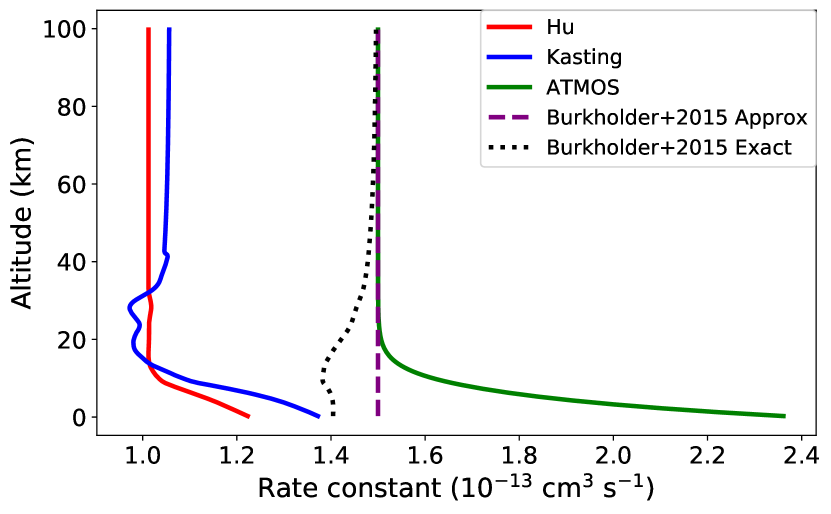
Figure 8: Different effective bimolecular rate laws for $CO+OH\rightarrow CO_{2}+H$ as a function of altitude in the T-P profile corresponding to this planetary scenario, calculated by ATMOS (see Figure 9). The lower atmosphere, where the H₂O photolysis rate is high and this reaction most important, is also where these rate laws most strongly disagree

C.2.2 S + CO Ratelaw

ATMOS includes the reaction $S+CO+M\rightarrow OCS+M$, with rate law equal to that of $O+CO+M\rightarrow CO_{2}+M$, following Mills (1998). This reaction has not been observed in the laboratory, but has been included as it is inferred from the atmospheric photochemistry of Venus, particularly the presence of OCS in its lower atmosphere (Krasnopolsky, 2007; Yung et al., 2009). Inclusion of this reaction decreases $r_{CO}$ by $20\%$, and supports $\sim$ppb levels of OCS. When this reaction is excluded, OCS essentially does not exist in the atmospheric scenarios we consider here. We identify this reaction as a key target for experimental characterization.

C.3 Atmospheric Profile

In anoxic, abiotic CO₂-rich atmospheres, the stratosphere is cold due to efficient line cooling by CO₂ and the absence of shortwave-absorbing stratospheric O₃ (from biogenic O₂) or haze (from biogenic CH₄) (Kasting et al., 1984; Roble, 1995; Wordsworth & Pierrehumbert, 2013; Rugheimer & Kaltenegger, 2018). Cold stratospheres are dry, due to the low saturation pressure of H₂O at low temperatures (Wordsworth & Pierrehumbert, 2013). If this fact is neglected (i.e. if the stratosphere is allowed to be relatively warm and moist), then vigorous H₂O photolysis in the wet upper atmosphere generates abundant OH which suppresses $r_{CO}$ regardless of assumptions on H₂O and CO₂ cross-sections. The baseline T/P profile in the ATMOS Archaean+haze template is warm ($\sim 230$ K) because it was calculated for conditions in which shortwave absorption due to haze heats the stratosphere. By contrast, at the low CH₄/CO₂ ratios expected for CO₂-dominated abiotic exoplanets, haze formation is not expected, and the stratosphere should be cold ($\sim 150-170$ K) and dry (DeWitt et al., 2009; Guzmán-Marmolejo et al., 2013; Arney et al., 2016). This means that when applying the Archaean+haze template from ATMOS to this planetary scenario, it is important to first re-calculate temperature-pressure profiles that are consistent with this scenario, e.g. by using the CLIMA module of ATMOS (Figure 9). Neglect of self-consistent climate can lead to overestimating upper-atmospheric [H₂O] (and hence H₂O photolysis rates) by 2-4 orders of magnitude.

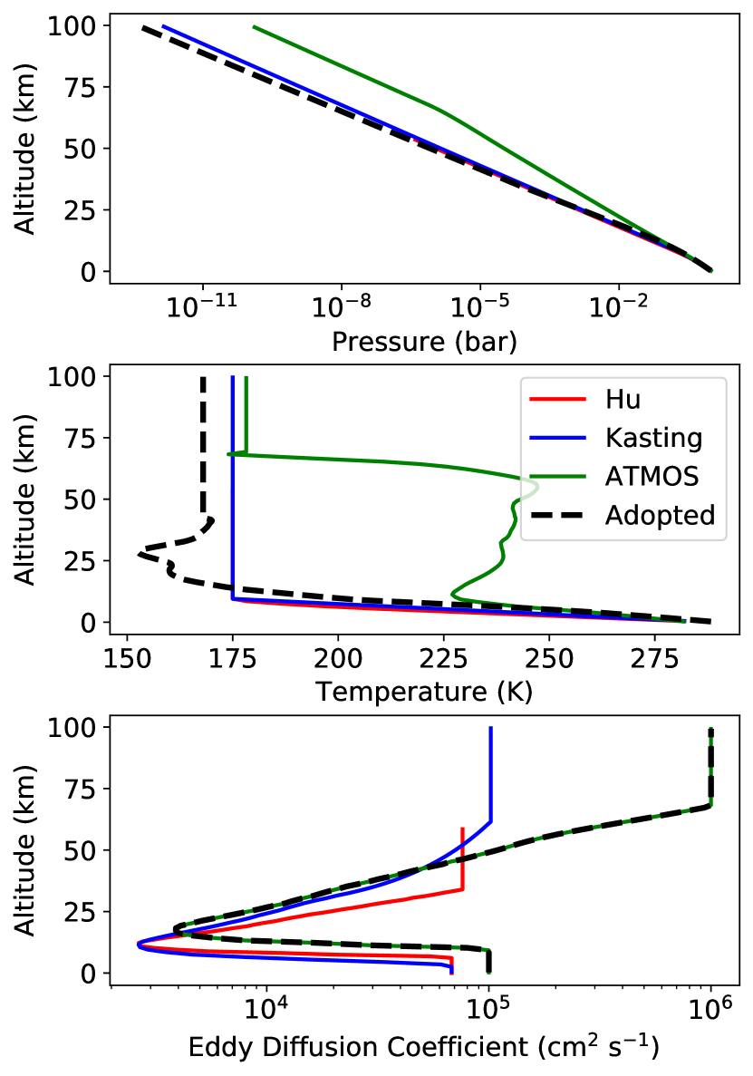
Figure 9: Pressure, temperature, and eddy diffusion coefficients as a function of altitude in the baseline models at project outset (solid colored lines; Hu et al. 2012; Harman et al. 2015; Arney et al. 2016). The original ATMOS T-P profile was derived from an unconverged haze run. Dashed black lines give these profiles as self-consistently calculated by ATMOS for the particular planetary scenario we consider here; these are the profiles adopted for purposes of intercomparison (c.f. Section C.5). It is crucial to include the cold stratosphere that results from the presence of CO₂ and the lack of shortwave absorbers; otherwise, the upper atmosphere is moistened and the H₂O photolysis rate is unphysically enhanced.

C.4 H and H₂ Escape Rates

Atmospheric H₂ stabilizes CO by suppressing OH and O (Kasting et al., 1983; Kharecha et al., 2005). In abiotic, anoxic atmospheres, pH₂ is generally set by a balance between H₂ outgassing and H and H₂ escape from the atmosphere, with the escape velocities calculated by:

$$v_{diff}=D(\frac{1}{H_{0}}-\frac{1}{H})$$

where $D(X,Y)$ is the molecular diffusion coefficient of $X$ through $Y$ in cm²s^-1, $H_{0}$ is the scale height for the bulk atmosphere at the escape altitude, $H$ is the scale height for the escaping component at the escape altitude, and $v_{diff}$ is the diffusion-limited escape velocity.

The calculation of $D(X,Y)$ for H and H₂ through CO₂ and through N₂ are different between the Hu, Kasting, and ATMOS models (Figure 10). Specifically, the Kasting model uses a generalized diffusion coefficient formulation, valid for an interaction radius of $3\times 10^{-8}$ cm (Banks & Kockart, 1973):

$$D_{i}=\frac{1.52\times 10^{18}\times(\frac{1}{\mu}+\frac{1}{\bar{\mu}})^{0.5}\times T^{0.5}\text{cm}^{-1}~{}\text{s}^{-1}}{n}$$ (C3)

where $\mu$ is the molecular weight of the individual species, $\bar{\mu}$ is the mean molecular weight of the atmosphere, $n$ is the number density in cm^-3, and $T$ is the temperature in K.

The Hu model uses individualized expressions for $D(X,Y)$. $D(H,N_{2})$ and $D(H_{2},N_{2})$ are taken from Banks & Kockart (1973). $D(H_{2},CO2)$ is taken from Marrero & Mason (1972), with the caveat that the exponential correction factor $\exp(\frac{-11.7K}{T})$ is evaluated at 175K, corresponding to the assumed stratospheric temperature in the CO₂-dominated case from Hu et al. (2012); this simplification leads to a $<4\%$ deviation from $150-300$ K. $D(H,CO_{2})$ is taken as $1.8\times D(H_{2},CO_{2})$ following the observation of Zahnle et al. (2008) that $D(H,He)=1.8\times D(H_{2},He)$:

$$D(H,CO_{2})=\frac{3.87\times 10^{17}T^{0.75}\text{cm}^{-1}~{}\text{s}^{-1}}{n}$$

$$D(H_{2},CO_{2})=\frac{2.15\times 10^{17}T^{0.75}\text{cm}^{-1}~{}\text{s}^{-1}}{n}$$

$$D(H,N_{2})=\frac{4.87\times 10^{17}T^{0.698}\text{cm}^{-1}~{}\text{s}^{-1}}{n}$$

$$D(H_{2},N_{2})=\frac{2.15\times 10^{17}T^{0.740}\text{cm}^{-1}~{}\text{s}^{-1}}{n}$$

The ATMOS model uses:

$$D(H,CO_{2})=\frac{2.0\times 10^{19}(T/200K)^{0.75}}{n}$$ (C4)

$$D(H_{2},CO_{2})=\frac{1.1\times 10^{19}(T/200K)^{0.75}}{n}$$ (C5)

$$D(H,N_{2})=\frac{2.7\times 10^{19}(T/200K)^{0.75}}{n}$$ (C6)

$$D(H_{2},N_{2})=\frac{1.4\times 10^{19}(T/200K)^{0.75}}{n}$$ (C7)

Figure 10 shows the variation in diffusion coefficient as a function of temperature for the formalisms selected by the different models. $nD$ does not vary significantly as a function of background gas for the Hu and Kasting models; however, $nD$ varies significantly as a function of background gas in ATMOS. By default, ATMOS uses coefficients for diffusion through N₂. Correcting these to the coefficients for diffusion through CO₂ (e.g., ATMOS “Mars” setting) results in a $1.5\times$ increase in pH₂ and a $2\times$ increase for $r_{CO}$. For diffusion through CO₂, the Kasting formalism leads to higher escape of H₂ (and hence lower pH₂ and $r_{CO}$) compared to the Hu and ATMOS models.

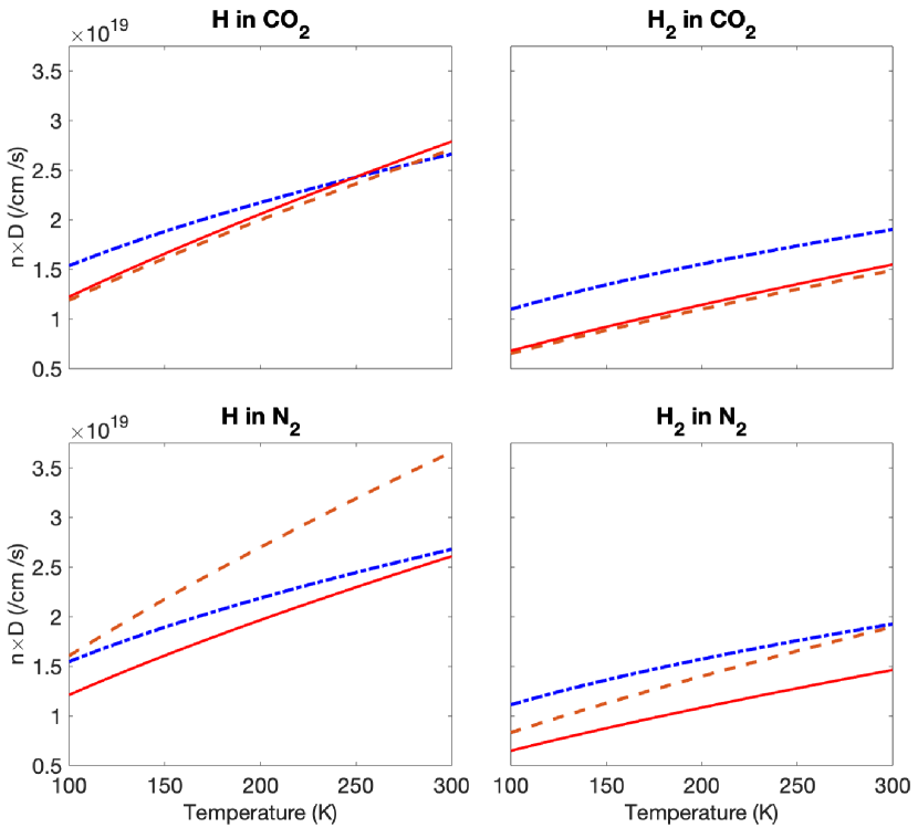
Figure 10: $nD(X,Y)$ from different models. Red curves correspond to the Hu model, blue to the Kasting model, and orange to ATMOS.

C.5 Demonstrating Model Agreement

To demonstrate that we have identified the key parameters driving the published variation in $r_{CO}$ between models, we run all three models under identical assumptions and show that our models agree and that we can reproduce both the high and low $r_{CO}$ published in the literature. Table 6 enumerates the conditions required to achieve high and low CO in our models. Table 7 lists the other parameters that must be aligned between the models. We note that the choices of the constant parameters (Table 7) are chosen primarily to facilitate the numerical experiment of the intercomparison, not for physical realism. For example, we essentially neglect rainout for purposes of this intercomparison; we do this not because CO₂-dominated rocky planets should lack rain, but because this is the most tractable rainout regime we can force all three of our models into, and because the results are not sensitive to this assumption. Similarly, when considering CO₂ absorption, we use cross-sections from the Kasting/ATMOS models, not because they are the most current estimates of CO₂ absorption, but because it is easier to incorporate these cross-sections into the Hu model than vice versa. Finally, we note that while that mixing length theory suggests the CO₂-dominated atmospheres should be more turgid than N₂-dominated atmospheres (Hu et al., 2012; Harman et al., 2015), using the Hu et al. (2012) eddy diffusion profile for CO₂-dominated atmospheres leads to numerical instabilities in the ATMOS and Kasting models. We consequently elect to use the ATMOS eddy diffusion profile, calibrated for N₂-dominated atmospheres, in this numerical experiment. It is unclear why reduced eddy diffusion should lead to such instabilities; we intend further studies to answer this question. Overall, we therefore emphasize that the use of these parameters should not necessarily constitute an endorsement, as they were primarily chosen to facilitate model intercomparison. The models were corrected for the errors summarized in Table 4, and the simulation parameters were otherwise as given in Tables 2 and  3.

Table 6: Parameters defining high and low CO cases (Hu et al. (2012) CO₂-dominated scenario) file

Scenario Parameter	High CO	Low CO
H2O cross-sections (ATMOS/Kasting)	Terminated at 198 nm	Extrapolated to 208.3 nm
H and H2 Diffusion Coefficient	Hu/ATMOS (CO2-dominated)	Kasting
CO + OH Ratelaw	Hu/Kasting	ATMOS
S + CO	No	Yes∗

Note. — ^∗The Kasting model (Harman et al., 2015) does not include OCS, and hence does not include this reaction

Table 7: Parameters held constant between high and low CO cases

Scenario Parameter	Hu	ATMOS	Kasting
Semimajor Axis		1.21 AU
TP Profile		Calculated from ATMOS (Fig. 9)
Eddy Diffusion		ATMOS (Fig. 9)
Surface Albedo		0.25
CO2 Cross-Sections		As in Kasting/ATMOS (Kasting & Walker, 1981)
Vertical Resolution		$0-100$ km, 1 km resolution
Lightning		Off
Rainout		$10^{-9}\times$ Earthlike
Global Redox Balance Enforced	No	No	No/Yes

The results of this numerical experiment are given in Table 8. Our models (1) agree with each other to within a factor of 2, and (2) can reproduce both the low ($\sim$200 ppm) and high ($\sim 8200$ ppm) CO surface mixing ratios published in the literature (e.g., Hu et al. 2012; Harman et al. 2015). Agreement between ATMOS and Hu is within $10\%$, reflecting particularly intensive intercomparison. We conclude that we have successfully identified the parameters driving divergent predictions of $r_{CO}$ in this planetary scenario.

Table 8: CO surface mixing ratios for the three models, applied to our abiotic CO₂-N₂ atmospheric scenario. The first line presents the mixing ratios from the models at the outset of the project, i.e. prior to fixing the errors in Table 4. $r_{CO}$ disagreed by $50\times$. The second and third line present the mixing ratios calculated from the models after fixing the errors, with uniform simulation parameters, under assumptions corresponding to both high and low CO (Tables 7, 6). Calculated $r_{CO}$ agreed within a factor of $2\times$ between models, demonstrating that we had successfully identified and accounted for the factors driving divergent $r_{CO}$ between models

Scenario Parameter	$r_{CO}$ (Hu)	$r_{CO}$ (ATMOS)	$r_{CO}$ (Kasting)
Initially	8.2E-3	1.72E-4	2.1E-4
Low-CO Assumptions	2.7E-4	2.6E-4	1.3E-4/1.5E-4∗
High-CO Assumptions	5.9E-3	5.4E-3	8.1E-3/8.2E-3∗

Note. — ^∗Global redox balance enforced as per Harman et al. (2015).

https://www.overleaf.com/project/5dd5a1ef1026ed0001d29c1b

References

- Ardaseva et al. (2017) Ardaseva, A., Rimmer, P. B., Waldmann, I., et al. 2017, MNRAS, 470, 187, doi: 10.1093/mnras/stx1012
- Arney et al. (2016) Arney, G., Domagal-Goldman, S. D., Meadows, V. S., et al. 2016, Astrobiology, 16, 873, doi: 10.1089/ast.2015.1422
- Badr & Probert (1995) Badr, O., & Probert, S. 1995, Applied energy, 50, 339
- Banks & Kockart (1973) Banks, P. M., & Kockart, G. 1973, Aeronomy (Part B) (New York, NY: Academic Press)
- Batalha et al. (2015) Batalha, N., Domagal-Goldman, S. D., Ramirez, R., & Kasting, J. F. 2015, Icarus, 258, 337, doi: 10.1016/j.icarus.2015.06.016
- Baulch et al. (1992) Baulch, D., Cobos, C., Cox, R., et al. 1992, Journal of Physical and Chemical Reference Data, 21, 411
- Benner et al. (2019) Benner, S. A., Kim, H.-J., & Biondi, E. 2019, Life, 9, 84
- Bohren (1987) Bohren, C. F. 1987, American Journal of Physics, 55, 524, doi: 10.1119/1.15109
- Brogi, M. et al. (2014) Brogi, M., de Kok, R. J., Birkby, J. L., Schwarz, H., & Snellen, I. A. G. 2014, A&A, 565, A124, doi: 10.1051/0004-6361/201423537
- Burkholder et al. (2015) Burkholder, J., Abbatt, J., Huie, R., et al. 2015, Chemical Kinetics and Photochemical Data for Use in Atmospheric Studies: Evaluation Number 18, Tech. rep., NASA Jet Propulsion Laboratory
- Cantrell et al. (1997) Cantrell, C. A., Zimmer, A., & Tyndall, G. S. 1997, Geophysical Research Letters, 24, 2195
- Catling & Kasting (2017) Catling, D. C., & Kasting, J. F. 2017, Atmospheric evolution on inhabited and lifeless worlds (Cambridge University Press)
- Chan et al. (1993) Chan, W. F., Cooper, G., & Brion, C. E. 1993, Chemical Physics, 178, 387, doi: 10.1016/0301-0104(93)85078-M
- Chung et al. (2001) Chung, C.-Y., Chew, E. P., Cheng, B.-M., Bahou, M., & Lee, Y.-P. 2001, Nuclear Instruments and Methods in Physics Research Section A: Accelerators, Spectrometers, Detectors and Associated Equipment, 467, 1572
- Citron et al. (2018) Citron, R. I., Manga, M., & Hemingway, D. J. 2018, Nature, 555, 643
- Cleaves (2008) Cleaves, H. J. 2008, Precambrian Research, 164, 111
- Darwent (1970) Darwent, B. d. B. 1970, Bond dissociation energies in simple molecules, Tech. rep., National Bureau of Standards (U.S.)
- DeMore et al. (1992) DeMore, W., Sander, S., Golden, D., et al. 1992, JPL Publication 92-20, Tech. rep.
- DeWitt et al. (2009) DeWitt, H. L., Trainer, M. G., Pavlov, A. A., et al. 2009, Astrobiology, 9, 447, doi: 10.1089/ast.2008.0289
- Dittmann et al. (2017) Dittmann, J. A., Irwin, J. M., Charbonneau, D., et al. 2017, Nature, 544, 333, doi: 10.1038/nature22055
- Domagal-Goldman et al. (2014) Domagal-Goldman, S. D., Segura, A., Claire, M. W., Robinson, T. D., & Meadows, V. S. 2014, ApJ, 792, 90, doi: 10.1088/0004-637X/792/2/90
- Dressing & Charbonneau (2015) Dressing, C. D., & Charbonneau, D. 2015, Astrophysical Journal, 807, 45, doi: 10.1088/0004-637X/807/1/45
- France et al. (2013) France, K., Froning, C. S., Linsky, J. L., et al. 2013, The Astrophysical Journal, 763, 149
- Fujii et al. (2018) Fujii, Y., Angerhausen, D., Deitrick, R., et al. 2018, Astrobiology, 18, 739, doi: 10.1089/ast.2017.1733
- Gaudi et al. (2020) Gaudi, B. S., Seager, S., Mennesson, B., et al. 2020, arXiv preprint arXiv:2001.06683
- Gilbert et al. (2020) Gilbert, E. A., Barclay, T., Schlieder, J. E., et al. 2020, arXiv preprint arXiv:2001.00952
- Gillon et al. (2017) Gillon, M., Triaud, A. H. M. J., Demory, B.-O., et al. 2017, Nature, 542, 456, doi: 10.1038/nature21360
- Graham et al. (1979) Graham, R. A., Winer, A. M., Atkinson, R., & Pitts, J. N. 1979, Journal of Physical Chemistry, 83, 1563
- Guzmán-Marmolejo et al. (2013) Guzmán-Marmolejo, A., Segura, A., & Escobar-Briones, E. 2013, Astrobiology, 13, 550, doi: 10.1089/ast.2012.0817
- Harman et al. (2018) Harman, C. E., Felton, R., Hu, R., et al. 2018, ApJ, 866, 56, doi: 10.3847/1538-4357/aadd9b
- Harman et al. (2013) Harman, C. E., Kasting, J. F., & Wolf, E. T. 2013, Origins of Life and Evolution of Biospheres, 43, 77
- Harman et al. (2015) Harman, C. E., Schwieterman, E. W., Schottelkotte, J. C., & Kasting, J. F. 2015, Astrophysical Journal, 812, 137, doi: 10.1088/0004-637X/812/2/137
- Hu & Diaz (2019) Hu, R., & Diaz, H. D. 2019, The Astrophysical Journal, 886, 126
- Hu et al. (2020) Hu, R., Peterson, L., & Wolf, E. T. 2020, ApJ, 888, 122, doi: 10.3847/1538-4357/ab5f07
- Hu et al. (2012) Hu, R., Seager, S., & Bains, W. 2012, Astrophysical Journal, 761, 166, doi: 10.1088/0004-637X/761/2/166
- Ityaksov et al. (2008) Ityaksov, D., Linnartz, H., & Ubachs, W. 2008, Chemical Physics Letters, 462, 31, doi: 10.1016/j.cplett.2008.07.049
- Jacob (1999) Jacob, D. J. 1999, Introduction to atmospheric chemistry (Princeton University Press)
- James & Hu (2018) James, T., & Hu, R. 2018, ApJ, 867, 17, doi: 10.3847/1538-4357/aae2bb
- Kasting (1990) Kasting, J. F. 1990, Origins of Life and Evolution of the Biosphere, 20, 199, doi: 10.1007/BF01808105
- Kasting (1993) —. 1993, Science, 259, 920, doi: 10.1126/science.259.5097.920
- Kasting (2013) Kasting, J. F. 2013, Chemical Geology, 362, 13
- Kasting (2014) —. 2014, Geological Society of America Special Papers, 504, 19
- Kasting et al. (1984) Kasting, J. F., Pollack, J. B., & Crisp, D. 1984, Journal of atmospheric chemistry, 1, 403
- Kasting & Walker (1981) Kasting, J. F., & Walker, J. C. 1981, Journal of Geophysical Research: Oceans, 86, 1147
- Kasting et al. (1983) Kasting, J. F., Zahnle, K. J., & Walker, J. C. G. 1983, Precambrian Research, 20, 121, doi: 10.1016/0301-9268(83)90069-4
- Keller-Rudek et al. (2013) Keller-Rudek, H., Moortgat, G. K., Sander, R., & Sörensen, R. 2013, Earth System Science Data, 5, 365, doi: 10.5194/essd-5-365-2013
- Kharecha et al. (2005) Kharecha, P., Kasting, J., & Siefert, J. 2005, Geobiology, 3, 53
- Kopparapu et al. (2013) Kopparapu, R. K., Ramirez, R., Kasting, J. F., et al. 2013, ApJ, 765, 131, doi: 10.1088/0004-637X/765/2/131
- Krasnopolsky (2007) Krasnopolsky, V. 2007, Icarus, 191, 25, doi: 10.1016/j.icarus.2007.04.028
- Krasnopolsky (2011) Krasnopolsky, V. A. 2011, Planet. Space Sci., 59, 952, doi: 10.1016/j.pss.2010.02.011
- Krissansen-Totton et al. (2018) Krissansen-Totton, J., Olson, S., & Catling, D. C. 2018, Science Advances, 4, eaao5747, doi: 10.1126/sciadv.aao5747
- Lightowlers & Cape (1988) Lightowlers, P., & Cape, J. 1988, Atmospheric Environment (1967), 22, 7
- Lustig-Yaeger et al. (2019) Lustig-Yaeger, J., Meadows, V. S., & Lincowski, A. P. 2019, AJ, 158, 27, doi: 10.3847/1538-3881/ab21e0
- LUVOIR Team (2019) LUVOIR Team, X. 2019, arXiv preprint arXiv:1912.06219
- Mancinelli & McKay (1988) Mancinelli, R. L., & McKay, C. P. 1988, Origins of Life, 18, 311, doi: 10.1007/BF01808213
- Marrero & Mason (1972) Marrero, T. R., & Mason, E. A. 1972, Journal of Physical and Chemical Reference Data, 1, 3
- McElroy & Donahue (1972) McElroy, M. B., & Donahue, T. M. 1972, Science, 177, 986
- Meadows et al. (2018) Meadows, V. S., Reinhard, C. T., Arney, G. N., et al. 2018, Astrobiology, 18, 630
- Meixner et al. (2019) Meixner, M., Cooray, A., Leisawitz, D., et al. 2019, arXiv e-prints, arXiv:1912.06213. https://arxiv.org/abs/1912.06213
- Mills (1998) Mills, F. P. 1998, Dissertation (ph.d.), California Institute of Technology, doi: 10.7907/NWPG-E852
- Mills & Allen (2007) Mills, F. P., & Allen, M. 2007, Planet. Space Sci., 55, 1729, doi: 10.1016/j.pss.2007.01.012
- Mota et al. (2005) Mota, R., Parafita, R., Giuliani, A., et al. 2005, Chemical Physics Letters, 416, 152, doi: 10.1016/j.cplett.2005.09.073
- Parkinson & Hunten (1972) Parkinson, T. D., & Hunten, D. M. 1972, Journal of Atmospheric Sciences, 29, 1380, doi: 10.1175/1520-0469(1972)029<1380:SAAOOO>2.0.CO;2
- Parkinson & Yoshino (2003) Parkinson, W., & Yoshino, K. 2003, Chemical Physics, 294, 31
- Parkinson et al. (2003) Parkinson, W. H., Rufus, J., & Yoshino, K. 2003, Chemical Physics, 290, 251, doi: 10.1016/S0301-0104(03)00146-0
- Prinn (1971) Prinn, R. G. 1971, Journal of Atmospheric Sciences, 28, 1058, doi: 10.1175/1520-0469(1971)028<1058:POHAOM>2.0.CO;2
- Prinn & Fegley Jr (1987) Prinn, R. G., & Fegley Jr, B. 1987, Annual review of earth and planetary sciences, 15, 171
- Quickenden & Irvin (1980) Quickenden, T., & Irvin, J. 1980, The Journal of Chemical Physics, 72, 4416
- Ranjan & Sasselov (2017) Ranjan, S., & Sasselov, D. D. 2017, Astrobiology, 17, 169, doi: 10.1089/ast.2016.1519
- Ranjan et al. (2019) Ranjan, S., Todd, Z. R., Rimmer, P. B., Sasselov, D. D., & Babbin, A. R. 2019, Geochemistry, Geophysics, Geosystems, 20, 2021
- Ranjan et al. (2017) Ranjan, S., Wordsworth, R., & Sasselov, D. D. 2017, The Astrophysical Journal, 843, 110. http://stacks.iop.org/0004-637X/843/i=2/a=110
- Ranjan et al. (2017) Ranjan, S., Wordsworth, R., & Sasselov, D. D. 2017, Astrobiology, 17, 687, doi: 10.1089/ast.2016.1596
- Reinhard et al. (2017) Reinhard, C. T., Olson, S. L., Schwieterman, E. W., & Lyons, T. W. 2017, ArXiv e-prints. https://arxiv.org/abs/1702.01137
- Ren et al. (2015) Ren, T., Modest, M. F., Fateev, A., & Clausen, S. 2015, Journal of Quantitative Spectroscopy and Radiative Transfer, 151, 198
- Rimmer & Helling (2016) Rimmer, P. B., & Helling, C. 2016, ApJS, 224, 9, doi: 10.3847/0067-0049/224/1/9
- Rimmer & Rugheimer (2019) Rimmer, P. B., & Rugheimer, S. 2019, Icarus, 329, 124
- Roble (1995) Roble, R. 1995, Reviews of Geophysics, 33, 539
- Rodler & López-Morales (2014) Rodler, F., & López-Morales, M. 2014, Astrophysical Journal, 781, 54, doi: 10.1088/0004-637X/781/1/54
- Rugheimer & Kaltenegger (2018) Rugheimer, S., & Kaltenegger, L. 2018, The Astrophysical Journal, 854, 19
- Rugheimer et al. (2015) Rugheimer, S., Kaltenegger, L., Segura, A., Linsky, J., & Mohanty, S. 2015, The Astrophysical Journal, 809, 57
- Rugheimer et al. (2015) Rugheimer, S., Segura, A., Kaltenegger, L., & Sasselov, D. 2015, Astrophysical Journal, 806, 137, doi: 10.1088/0004-637X/806/1/137
- Sander et al. (2003) Sander, S. P., Friedl, R. R., Ravishankara, A. R., et al. 2003, Chemical Kinetics and Photochemical Data for Use in Atmospheric Studies Evaluation Number 14, Tech. Rep. 14, NASA JPL. http://jpldataeval.jpl.nasa.gov/
- Sander et al. (2011) Sander, S. P., Friedl, R. R., Barker, J. R., et al. 2011, Chemical Kinetics and Photochemical Data for Use in Atmospheric Studies Evaluation Number 17, Tech. Rep. 17, NASA JPL. http://jpldataeval.jpl.nasa.gov/
- Sandor & Clancy (2018) Sandor, B. J., & Clancy, R. T. 2018, Icarus, 313, 15, doi: 10.1016/j.icarus.2018.04.022
- Sasselov et al. (2020) Sasselov, D. D., Grotzinger, J. P., & Sutherland, J. D. 2020, Science Advances, 6, doi: 10.1126/sciadv.aax3419
- Schaefer & Fegley (2011) Schaefer, L., & Fegley, Bruce, J. 2011, ApJ, 729, 6, doi: 10.1088/0004-637X/729/1/6
- Schulz et al. (2002) Schulz, C., Koch, J., Davidson, D., Jeffries, J., & Hanson, R. 2002, Chemical Physics Letters, 355, 82
- Schwieterman et al. (2019) Schwieterman, E. W., Reinhard, C. T., Olson, S. L., et al. 2019, ApJ, 874, 9, doi: 10.3847/1538-4357/ab05e1
- Schwieterman et al. (2016) Schwieterman, E. W., Meadows, V. S., Domagal-Goldman, S. D., et al. 2016, Astrophysical Journall, 819, L13, doi: 10.3847/2041-8205/819/1/L13
- Segura et al. (2005) Segura, A., Kasting, J. F., Meadows, V., et al. 2005, Astrobiology, 5, 706, doi: 10.1089/ast.2005.5.706
- Segura et al. (2007) Segura, A., Meadows, V. S., Kasting, J. F., Crisp, D., & Cohen, M. 2007, A&A, 472, 665, doi: 10.1051/0004-6361:20066663
- Shkolnik & Barman (2014) Shkolnik, E. L., & Barman, T. S. 2014, AJ, 148, 64, doi: 10.1088/0004-6256/148/4/64
- Snellen et al. (2010) Snellen, I. A. G., de Kok, R. J., de Mooij, E. J. W., & Albrecht, S. 2010, Nature, 465, 1049, doi: 10.1038/nature09111
- Stachnik & Molina (1987) Stachnik, R., & Molina, M. 1987, Journal of Physical Chemistry, 91, 4603
- Tan et al. (1978) Tan, K. H., Brion, C. E., van der Leeuw, P. E., & van der Wiel, M. J. 1978, Chemical Physics, 29, 299
- Thompson et al. (1963) Thompson, B., Harteck, P., & Reeves Jr, R. 1963, Journal of Geophysical Research, 68, 6431
- Tian et al. (2014) Tian, F., France, K., Linsky, J. L., Mauas, P. J. D., & Vieytes, M. C. 2014, Earth and Planetary Science Letters, 385, 22, doi: 10.1016/j.epsl.2013.10.024
- Torres et al. (2015) Torres, G., Kipping, D. M., Fressin, F., et al. 2015, ApJ, 800, 99, doi: 10.1088/0004-637X/800/2/99
- Walker (1974) Walker, J. C. 1974, American Journal of Science, 274, 193
- Wang & Hou (2005) Wang, B., & Hou, H. 2005, Chemical physics letters, 410, 235
- Wang et al. (2016) Wang, Y., Tian, F., Li, T., & Hu, Y. 2016, Icarus, 266, 15, doi: 10.1016/j.icarus.2015.11.010
- Way et al. (2016) Way, M. J., Del Genio, A. D., Kiang, N. Y., et al. 2016, Geophysical Research Letters, 43, 8376, doi: 10.1002/2016GL069790
- Wogan & Catling (2020) Wogan, N. F., & Catling, D. C. 2020, ApJ, 892, 127, doi: 10.3847/1538-4357/ab7b81
- Wolf (2017) Wolf, E. T. 2017, The Astrophysical Journal Letters, 839, L1
- Wong et al. (2017) Wong, M. L., Charnay, B. D., Gao, P., Yung, Y. L., & Russell, M. J. 2017, Astrobiology, 17, 975, doi: 10.1089/ast.2016.1473
- Wordsworth & Pierrehumbert (2014) Wordsworth, R., & Pierrehumbert, R. 2014, Astrophysical Journall, 785, L20, doi: 10.1088/2041-8205/785/2/L20
- Wordsworth (2016) Wordsworth, R. D. 2016, Annual Review of Earth and Planetary Sciences, 44, 381, doi: 10.1146/annurev-earth-060115-012355
- Wordsworth & Pierrehumbert (2013) Wordsworth, R. D., & Pierrehumbert, R. T. 2013, ApJ, 778, 154, doi: 10.1088/0004-637X/778/2/154
- Yung & Demore (1982) Yung, Y. L., & Demore, W. B. 1982, Icarus, 51, 199, doi: 10.1016/0019-1035(82)90080-X
- Yung et al. (2009) Yung, Y. L., Liang, M. C., Jiang, X., et al. 2009, Journal of Geophysical Research, 114, E00B34, doi: 10.1029/2008JE003094
- Zahnle et al. (2008) Zahnle, K., Haberle, R. M., Catling, D. C., & Kasting, J. F. 2008, Journal of Geophysical Research (Planets), 113, E11004, doi: 10.1029/2008JE003160