Solving the scalarization issues of Advantage-based Reinforcement Learning Algorithms
Abstract
In this research, some of the issues that arise from the scalarization of the multi-objective optimization problem in the Advantage Actor Critic (A2C) reinforcement learning algorithm are investigated. The paper shows how a naive scalarization can lead to gradients overlapping. Furthermore, the possibility that the entropy regularization term can be a source of uncontrolled noise is discussed. With respect to the above issues, a technique to avoid gradient overlapping is proposed, while keeping the same loss formulation. Moreover, a method to avoid the uncontrolled noise, by sampling the actions from distributions with a desired minimum entropy, is investigated. Pilot experiments have been carried out to show how the proposed method speeds up the training. The proposed approach can be applied to any Advantage-based Reinforcement Learning algorithm.
keywords:
Reinforcement Learning , Actor Critic , Deep Learning , Gradient-based optimizationSee pages - of ./img/citation.pdf
1 Introduction and formal background
1.1 Introduction
In last years, unprecedented results has been achieved in the Reinforcement Learning (RL) research field with the use of Artificial Neural Networks (ANNs). In essence, in an RL model an agent interacts with its environment and, upon observation of the consequences of its actions, learns to adapt its own behaviour to rewards received. An agent behavior is modelled in terms of state-action relationships. The goal of the agent is to learn a control strategy (i.e., a policy) maximizing the total reward. An important advancement in the field has been the possibility to operate with high-dimensional state and action spaces via Deep Learning [1].
More specifically, policy gradient models optimize the policy, represented as a parameterized function, via gradient-descent optimization. An increasing interest of the research community has recently led to the paradigm shift of multi-objective reinforcement learning (MORL), in which learning control policies are simultaneously optimized over several criteria [2] [3].
In RL Advantage learning is used to estimate the advantage of performing a certain action. [4] Consequently, in the Actor-Critic (AC) method a value function(which measures the expected reward) is learned in addition to the policy, in order to assist the policy update [5]. This model is based on a “Critic”, which estimates the value function, and an “Actor”, which updates the policy distribution in the direction suggested by the “Critic” [6].
This research work focuses on some significant issues of the Advantage Actor Critic (A2C) algorithm, that arise from the scalarization of the multi-objective optimization problem. Firstly, it shows that a naive scalarization can lead to gradients overlapping. Secondly, it investigates the possibility that the entropy regularization term can inject uncontrolled noise. With respect to such issues, a technique to avoid gradient overlapping (called Non-Overlapping Gradient, NOG) is proposed, which keeps the same loss formulation. Moreover, a method to avoid the uncontrolled noise, by sampling the actions from distributions with a desired minimum entropy (called Target Entropy, TE), is investigated. Experimental results compare the A2C algorithm with the proposed combination of A2C with NOG and TE (A2CNOG+TE).
With regard to performance evaluation, we carried out the hyperparameters optimization for each scenario over the same task [7]. Then using the best hyperparameters, we computed the confidence intervals over multiple runs.
As a relevant result, the combination of TE and NOG determines a decrease of the training time necessary to solve the problem. Specifically, the proposed technique achieves a larger speedup for increasing problem complexity.
The algorithmic design of the proposed approach is compliant with any Advantage-based Reinforcement Learning algorithm derived from A2C that share the same loss function components. The A2CNOG+TE algorithm has been developed, tested and publicly released on the Github platform, to foster its application on various research environments.
1.2 Formal background
An RL problem defines an environment representing a task. The objective of an RL algorithm is to find an optimal policy that an agent has to follow to solve the task. The environment can be represented as a Markov Decision Process (MDP). Denoting by the state space, and by the action space, it can be defined: (i) the state transition function ; (ii) the reward function .
The objective of an RL algorithm is then to find a policy such that following its trajectories the cumulative sum of the rewards for any starting state is maximized.
Usually, the policy is stochastic: is a function that, for each state , returns the probability of each action , i.e., . By using we assume that is the action sampled from a categorical distribution with probabilities , and is the probability of the action in the distribution . Under such assumption, the objective is to maximize the expectation of the cumulative sum of the rewards, i.e., .
In the literature, if the policy is approximated using an ANN, the term Deep Reinforcement Learning is used. RL algorithms are divided into two major categories: off-policy and on-policy [8]. The off-policy algorithms use stochastic techniques, for example , to explore the state space. In the first phase, such algorithms perform random actions and accumulate the transactions in a replay memory. In the second phase, the off-policy algorithms sample some transactions from the replay memory, and use them to train the policy. In contrast, the on-policy algorithms explore the space by following the policy and updating it via the current transactions without a replay memory.
In this paper we focus on the issues that arise in a family of on-policy algorithms.
1.3 The Advantage Actor Critic (A2C) Algorithm
The Advantage Actor Critic (A2C) algorithm, proposed by OpenAI, is the synchronous version of the Asynchronous Advantage Actor Critic (A3C) algorithm, proposed by Google [6]. It has been shown that A2C has the same performance of A3C but with a lower implementation and execution complexity.
A2C is based on the REINFORCE algorithm [5]. Let us define, for each time step , the future discounted cumulative reward . In the REINFORCE algorithm, each optimization step tends to maximize the expectation . Let us denote the parameters of . The REINFORCE algorithm follows the optimization trajectory defined by , which is an unbiased estimation of 111This is known as the log derivative trick..
Usually, the quantity has an high variance, and the optimization trajectories defined by are very noisy. To overcome this issue a baseline is used to reduce the variance, and the gradient is computed. A classical baseline can be the mean of .
The contributions of A2C to REINFORCE are twofold: to use an ANN approximating as the baseline , and to use this ANN to bootstrap the computation in partially observed environmental trajectories.
In REINFORCE can be computed after the end of the episode. In contrast, in A2C the estimates , and this value can be used to estimate the future discounted cumulative reward before the end of the episode. Therefore, A2C performs an optimization step every steps, without waiting for the end of the episode. A visual representation of this difference is given in Figure 1. Here, each box represents the current reward whereas represents the future total discounted cumulative reward. In the case of A2C, the future total discounted cumulative reward is computed via the available cumulative reward and an estimation of of the last available state using .

(right)
Overall, the remainder of this paper is structured as follows. Section 2 is devoted to the scalarization issues of the A2C algorithm. The proposed A2CNOG+TE algorithm is presented in Section 3. Experimental studies are covered by Section 4. Finally, Section 5 summarizes the major achievements and future work.
2 Scalarization issues of the A2C algorithm
The A2C algorithm uses two ANNs to approximate the two functions and . As previously stated, in A2C the environment is observed only for steps (instead of waiting for the episode termination). Given the partial state-action-reward observation, the algorithm computes, for each :
-
1.
using as bootstrap: ;
-
2.
The policy gradient ;
-
3.
The gradient ;
-
4.
The entropy gradient .
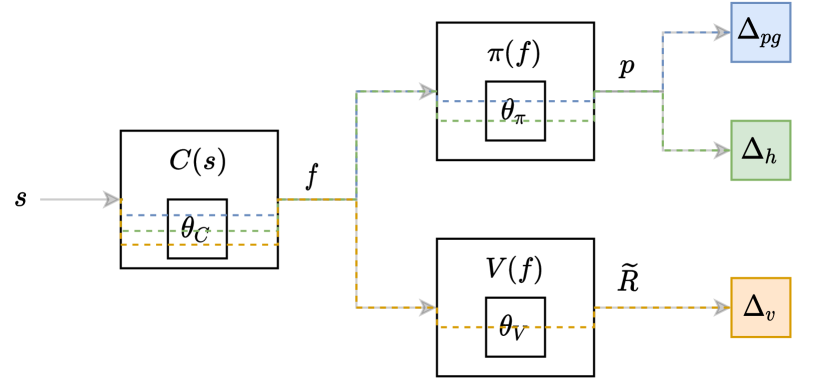
Subsequently, an optimization step is performed in the direction that maximizes both (direction ) and the entropy of (direction ), as well as minimizes the mean squared error of (direction ). It is a multi-objective optimization problem, which in the A2C algorithm has been solved with a scalarization. There are three different objectives, with some common parameters. Both the entropy and policy gradients share .
Also and often have some common parameters, because usually a feature extraction is performed on the state , and the features are used as inputs for and . Let us denote the feature extraction function, with its parameters, the features. By substituting with in in the and domains 333, and , then the computed gradients are:
| (1) | ||||
| (2) | ||||
| (3) |
where is the policy gradient, is the error gradient for the estimator net , and is a gradient of the entropy of the policy net. The notation represents the gradient of the argument with respect to and .
An optimization step is performed in the direction of the scalarized objective , where and are coefficients introduced to weight the strength of the entropy regularization term and of the gradient, respectively. It is apparent that all the three objective functions share some parameters. Specifically, the gradient computed for the parameter contains the contributions of and . Furthermore, the gradient for the parameter contains the contributions of , and .
A representation of the mutual dependency between gradients via related parameters is given in Figure 2.
Each coloured box represents a different gradient contribution to the overall loss related to: the policy , the entropy , and the total discounted cumulative reward estimator . Here, each big box represents a different Neural Network (NN), whereas the inner small box represents its parameters (i.e. a connection weights). In Figure, the input and output of each NN are also represented: is fed by the state to extract the features , whereas both the policy NN and the estimator NN take the features as an input, to provide the action probability vector and the future cumulative discounted reward estimate , respectively. In particular, each gradient is represented with a different color, and a dashed colored arrow from the gradient to the inputs highlights the backward path and thus the influence of a gradient to a parameter optimization. It is apparent that the sub-objectives are not independent, since they have common parameters. We call gradient overlapping this dependency among gradients. As a consequence, the policy and value function parameters can be pushed to sub-optimal regions.
Another issue that is considered in this research is the possibility that the entropy regularization term could generate noise in the network parameters. Indeed, it can be observed in Formula 3 that the gradient is not computed to reach a target entropy level, but just for increasing it.
In the next section the two issues are tackled considering also their reciprocal impact on the system performance.
3 The Proposed A2CNOG+TE algorithm
In this section a solution to avoid the gradient overlapping when using the A2C scalarized objective function is proposed. It is worth noting that to solve the gradient overlapping problem also allows to remove the weights coefficients of the scalarized objective function, thus reducing the hyperparameters search space, and then the optimization time. In the following, this approach will be referred to as the Non-Overlapping Gradient (NOG). Furthermore, an idea to solve the noise generated by the entropy regularization term is discussed. The idea is to maintain the entropy of the policy above a target level without using any gradient. In the following, this approach will be referred to as the Target Entropy (TE). As an effect, this can further reduce the gradient overlapping phenomenon.
3.1 Non-Overlapping-Gradients (NOG)
The NOG technique consists in simplifying the backward computation flow represented in Fig. 2, to remove the gradient overlapping on the feature extraction function , and to constrain the computation to the semantically appropriate functions. Specifically, the only gradient contributing to the feature extraction function optimization is . Similarly, the gradient should contribute just to the policy function optimization, as well as the gradient should contribute just to the value function optimization. According to such criterion, the new computed gradients are the following:
| (4) | ||||
| (5) | ||||
| (6) |
where, with respect to Formulas 1, 2, 3, and are computed respectively against and only.
This way, the gradient overlapping is sensibly reduced, but not totally disappeared. Specifically in this scenario the gradients and still overlap via the parameters of the policy function . A visual representation of the new gradient computation is given in Figure 3, where a colored cross represents where the backward computation of the related gradient component stops.
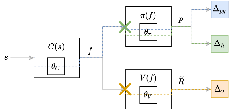
Using the Non Overlapping Gradients technique the new scalarized objective function is . Note that the parameter is not needed because is totally independent.
3.2 Target Entropy (TE)
In the previous section, it has been highlighted that the gradient is not computed to reach a target entropy level but just for increasing it. This can produce noise in the network parameters. In this section we propose a novel technique to maintain the entropy of the policy above a target level without using any gradient. As a consequence, the gradient overlapping can be completely removed when using the TE technique in conjunction with NOG.
Let us denote the probabilities of each action given the features of the state , and the highest probability. Let us observe that . Let us define as:
| (7) |
The property is maintained 444, i.e., is still a valid categorical distribution. It is also important to notice that .
Let us recall the definition of entropy , and let us focus on just one of the entropy components . It can be easily compute the difference of one contribution in function of . Considering the overall entropy difference , it can be written in function of contributions, as follows:
Rearranging the terms, can be rewritten as:
Expressing it in function of :
Let us assume that is small and close to zero. The Taylor expansion of where can be computed as follows:
Finally, by substituting back the approximation of in , the following approximation can be derived:
Using the above formula, can be computed as follows, in order to achieve a desired entropy of :
| (8) |
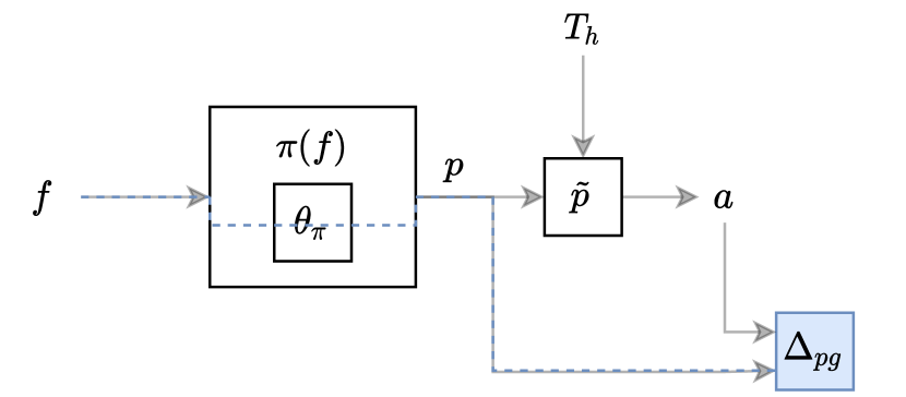
As a consequence, the action can be sampled from instead of , i.e., to sample the action from a categorical distribution with an entropy higher than . It is worth to notice that the action from the distribution can still be sampled using the gradient computation represented in Figure 4. As a result, the technique allows to keep a certain exploration over exploitation ratio, and at the same time it avoids raising entropy.
Using the Target Entropy technique, the new scalarized objective function is . It can be noted that there is no term. Figure 4 represents the resulting backward computation. Here, the focus is on the NN , whose output is now transformed using the Target Entropy according to 7 and 8. The resulting is used to sample an action . As a result, there is no more a contribution to the gradient related to . Then, the scalarization coefficients are not needed, because there are only two independent contributions to the gradient.
In the next section, the advantages of the NOG and TE techniques are experimentally evaluated.
4 Experimental Studies
In order to investigate the combined effect of the NOG and TE techniques, two different algorithms have been experimented:
-
1.
Classical A2C (A2C)
-
2.
A2C with Non-Overlapping-Gradients and Target Entropy (A2CNOG+TE)
For each training algorithm, first a hyperparameters optimization has been carried out. Subsequently, the best hyperparameters have been used to calculate the confidence interval, over 10 runs, of the training time needed to solve the problem.
To perform the experiments, three environments sufficiently complex to solve, which allow the hyperparameters optimization in a reasonable time, have been considered: EnergyMountainCar, CartPole and LunarLander, all from OpenAI Gym [9].
4.1 Hyperparameters Optimization
Table 1 shows the hyperparameters to optimize, for the considered algorithms. In order to sample the hyperparameters to use for each run, it has been used the Tree-structured Parzen Estimator (TPE) [7], whereas to prune unpromising runs it has been used the Successive Halve Pruning (SHP) [10]. More precisely every 1000 steps the current reward EMA (Exponential Moving Average) is reported to the SHP pruner.
| Name | Range | Sampling | Description |
| Categorical | Discount factor | ||
| Categorical | Env. steps for training step | ||
| lr | LogUniform | Learning rate | |
| mcn | Uniform | Max gradient clip norm | |
| LogUniform | strength | ||
| Uniform | strength | ||
| Uniform | Target Entropy |
Each run has been evaluated for 100 episodes, and the mean reward has been used as objective function (to maximize) for the hyperparameters optimization. All hyperparameters optimization has been run on an Intel Xeon with 40 cores. It follows, for each environment, a brief description, the results of the hyperparameters optimization, and the performance evaluation for the two comparative algorithms.
4.2 The EnergyMountainCar environment
In EnergyMountainCar a car drives up a hill which is steep with respect to its engine. Since the car is positioned in a valley, the agent must learn to drive back and forth to build up momentum. Figure 5 shows the environment and its control variables.
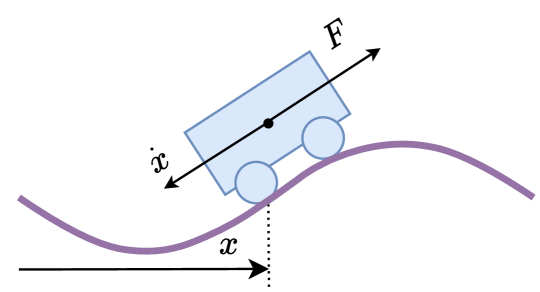
Specifically, the state space has 2 components: car’s horizontal position () and horizontal speed (). Three different actions can be performed by the agent: no action, accelerate () to the left or to the right. The reward is computed as the car’s total energy difference (potential and kinetic) of the last time step.
An episode finishes when the car reaches the top of the right hill. The goal is to spend less energy as possible. The environment is considered solved by achieving a cumulative reward of 0.45 points.
Figure 6 shows the objective value of the hyperparameters optimization process, against the number of trials sampled, for the comparative algorithm. The running best objective value is highlighted by a continuous line. In particular, it can be noted that the best objective value is immediately achieved by the A2CNOG+TE, whereas it is achieved at the fifth iteration by the A2C.
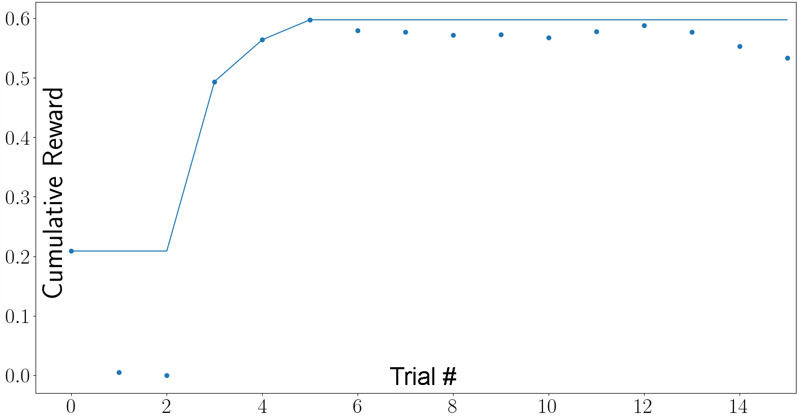
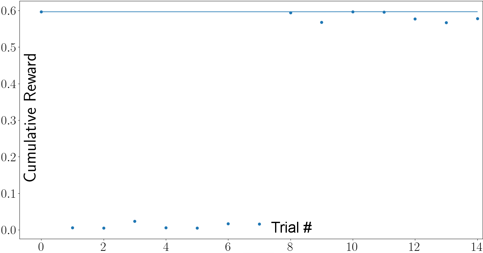
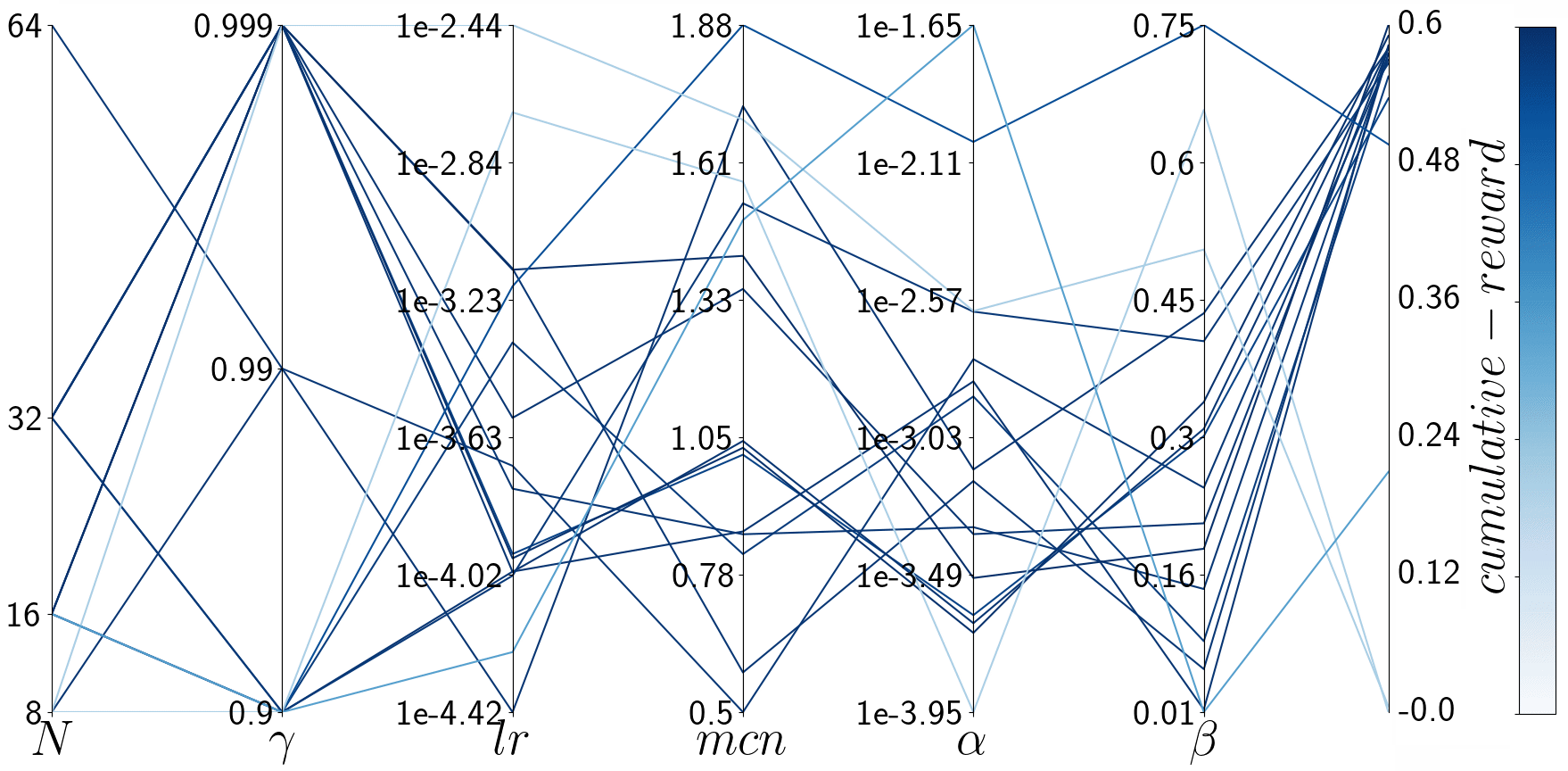
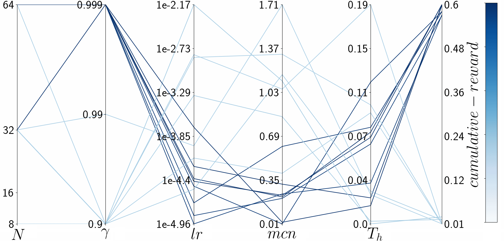
Figure 7 represents the hyperparameters values optimization and the related objective value, for the two algorithms. Here, each line represents a trial, with its hyperparameters values represented on the vertical axes. According to the colorbar, the blue level of the line allows to distinguish the best solutions. Here, it can be observed that the hyperparameters values corresponding to the highest objective values are more scattered for the A2C.
For the sake of completeness, Table 2 shows the best hyperparameters value for each considered algorithm.
| parameter | A2C | A2CNOG+TE |
| 0.999 | 0.999 | |
| 16 | 64 | |
| lr | 0.0007139 | 0.00003798 |
| max-clip-norm | 1.419 | 0.2302 |
| 0.0003160 | ||
| 0.1833 | ||
| 0.0739 |
After setting the best hyperparameters for each algorithm, the training process has been carried out 10 times for both algorithms.
Figure 8 shows the episode reward versus the training step for each algorithm, with its confidence interval. Precisely, the steps to solve the problem via the proposed A2CNOG+TE algorithm and via the classical A2C are and , respectively. The proposed approach improves the time efficiency of the A2C, up to more than 1.08x of average speedup.
4.3 The CartPole environment
CartPole, also known as inverted pendulum, is a pendulum with the center of mass above its pivot point. Figure 9 shows the environment and its control variables. The pivot point is an axis of rotation mounted on a cart, limiting the pendulum to one degree of freedom, along which the cart can move horizontally. Any displacement from the vertical position causes a gravitation torque and a consequent fall, if not balanced by the cart movement. The agent controls the cart in order to prevent the pendulum from falling, by applying a force of . The state space is represented by 4 components: cart position (), cart velocity (), pole angle (), and pole tip angular velocity (). The action space is two-dimensional: moving left or right. A reward of +1 is provided for every timestep with the pole upright. An episode ends when the pole is more than 15 degrees from vertical, or when the cart moves more than 2.4 units from the start. The goal is to keep the pole upright as much as possible. The environment is considered solved by achieving a cumulative reward of 195 points.
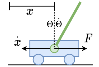
Figure 10 shows the objective value of the hyperparameters optimization process, against the number of trials sampled, for the comparative algorithm. It is worth noting that, there is a lower number of trials in the hyperparameters optimization of A2C. Specifically, during the optimization, there are unpromising trials which are aborted during the training process by the pruning algorithm. The figures clearly show that the A2C has been more affected by pruning with respect to the A2CNOG+TE.
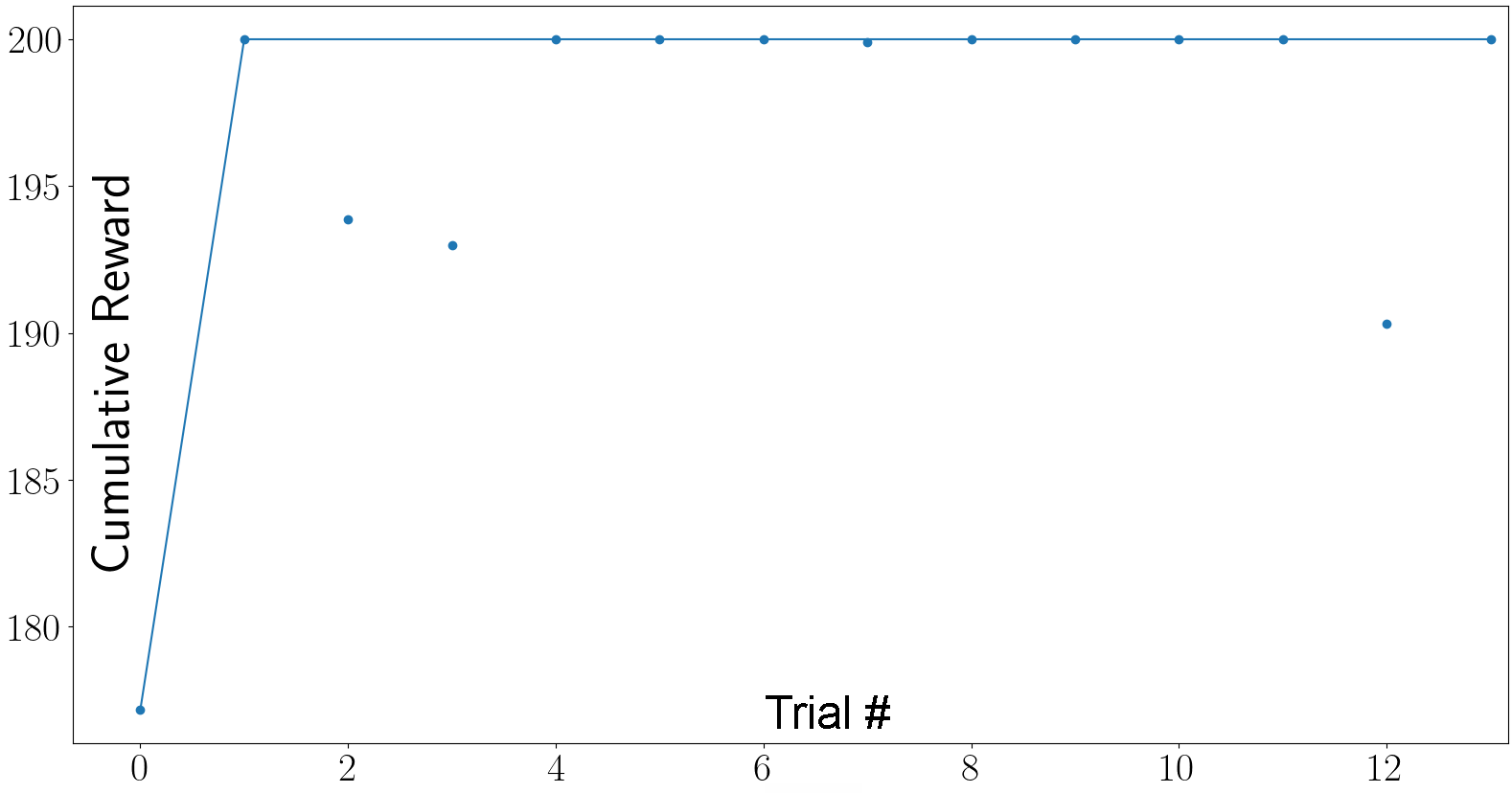
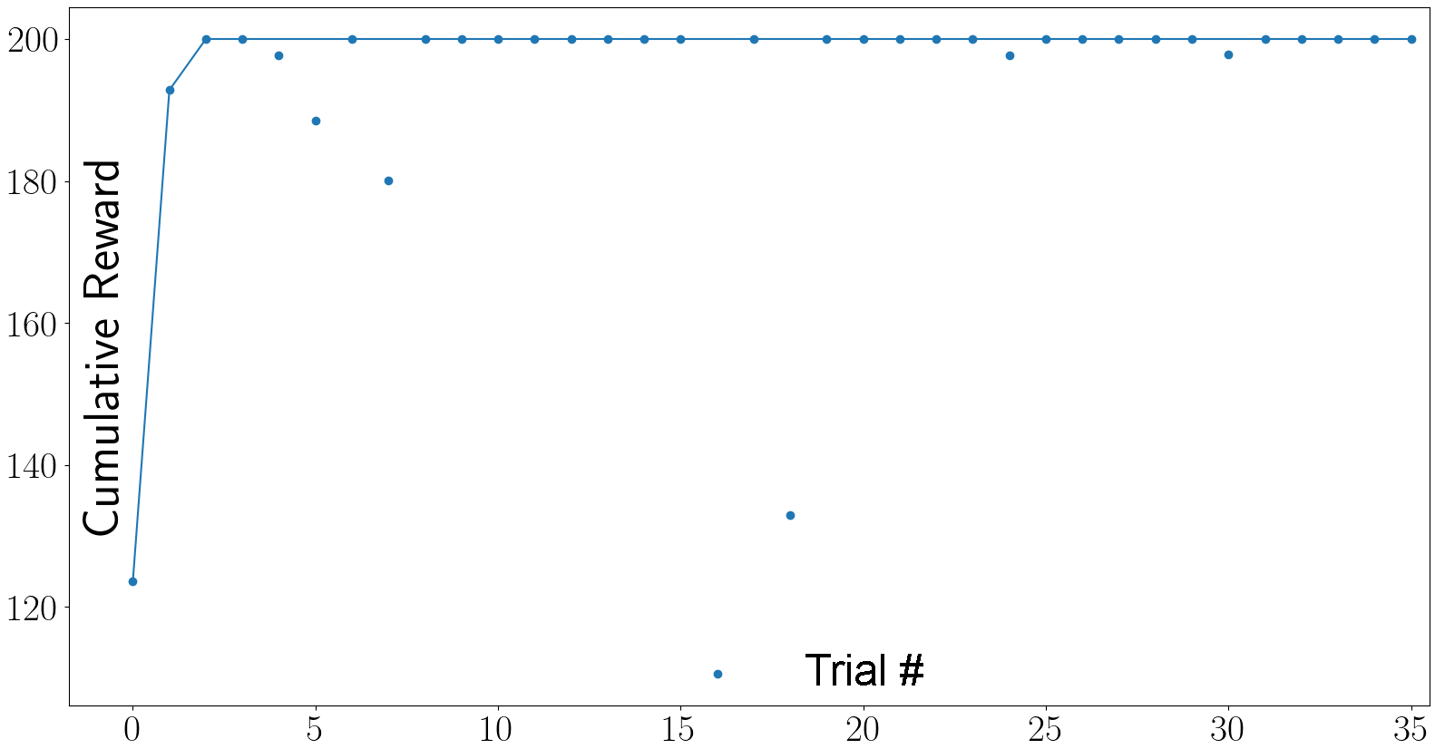
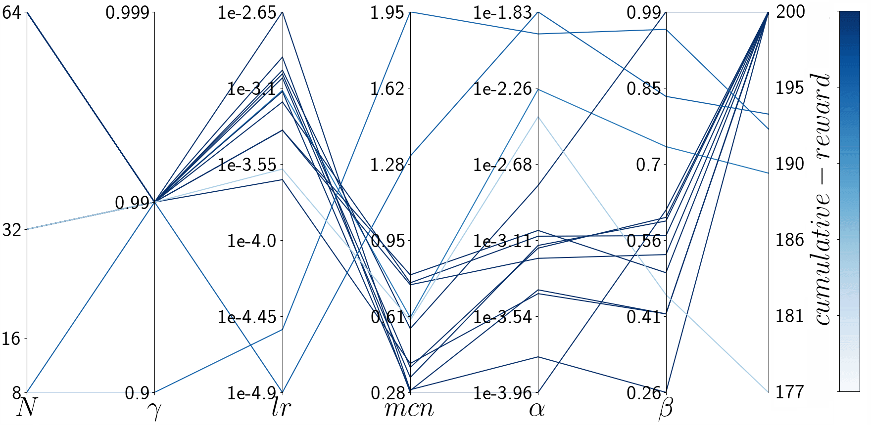
Figure 11 represents the hyperparameters values optimization and the related objective value, for the two algorithms. Here, each line represents a trial, with each hyperparameter value represented on the vertical axes. According to the colorbar, the blue level of the line allows to distinguish the best solutions. Here, it can be observed that for some hyperparameters values there is a higher density of good trials.
For the sake of completeness, Table 3 shows the best hyperparameters value for both algorithms.
| parameter | A2C | A2CNOG+TE |
| 0.99 | 0.99 | |
| 64 | 64 | |
| lr | 0.0009591 | 0.001642 |
| max-clip-norm | 0.3898 | 1.3569 |
| 0.0006986 | ||
| 0.5996 | ||
| 0.166 |
After setting the best hyperparameters for each algorithm, the training process has been carried out 10 times for each algorithm.
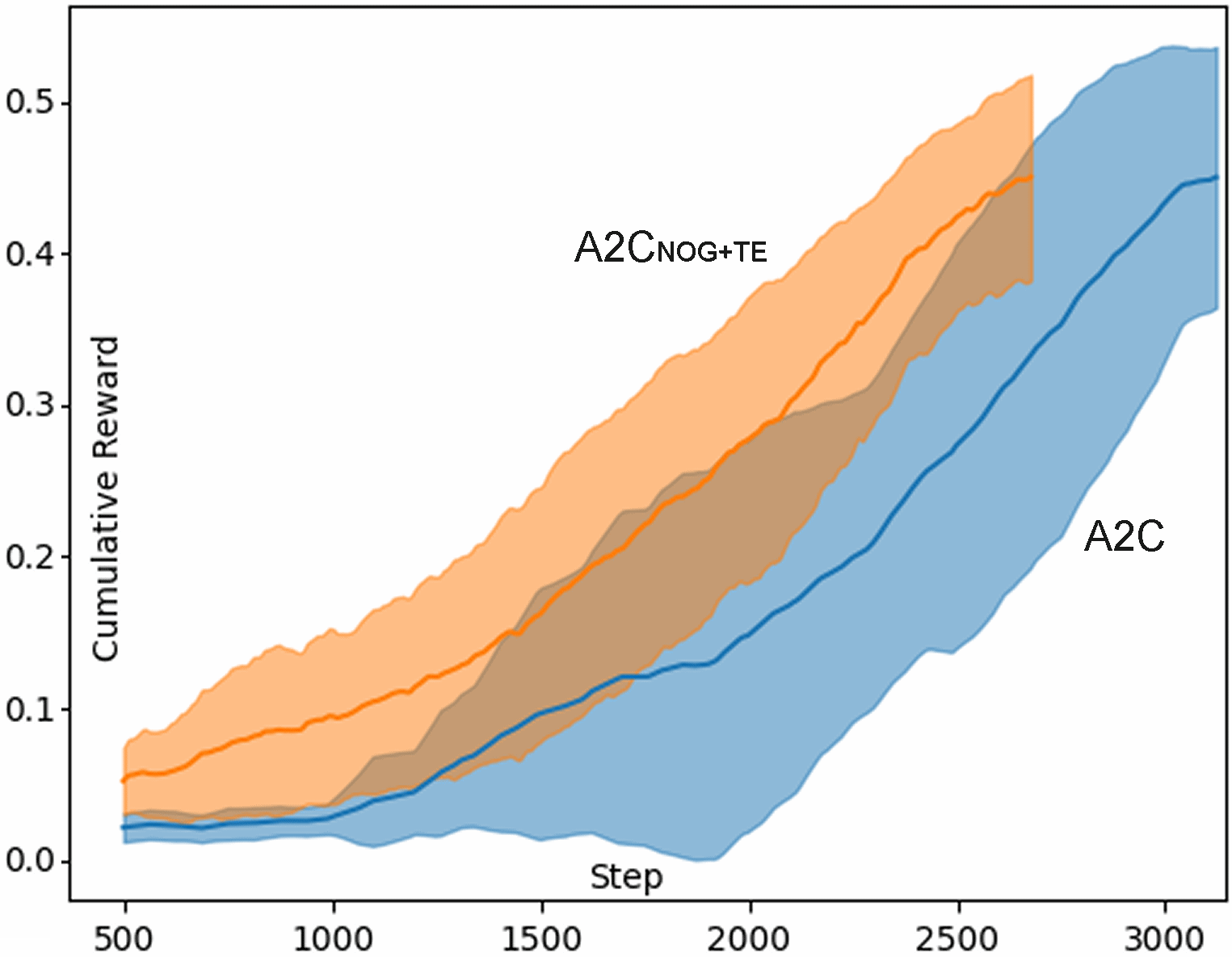
Figure 12 shows the episode reward versus the training step for each algorithm, with its confidence interval. Precisely, the steps to solve the problem via the proposed A2CNOG+TE algorithm and via the classical A2C are and , respectively. The proposed approach sensibly improves the time efficiency of the A2C, up to more than 1.18x of average speedup.
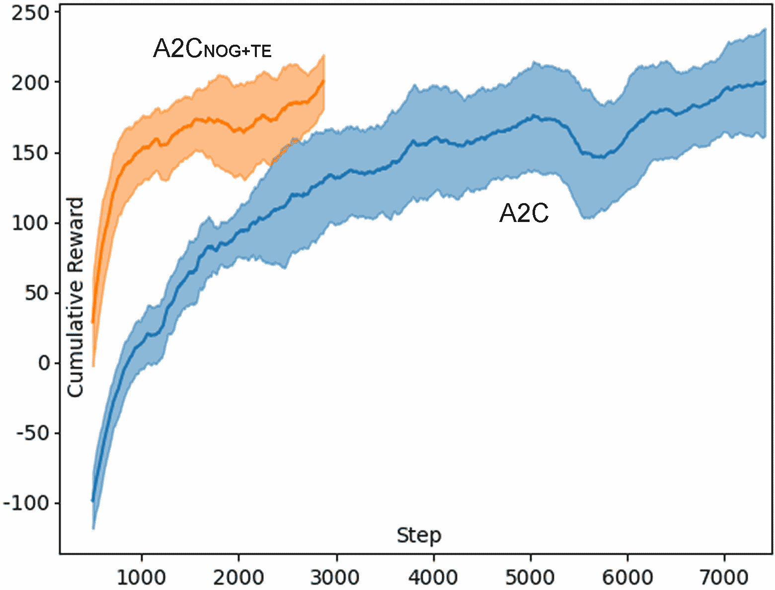
4.4 The LunarLander environment
LunarLander is a control task, in which the agent controls the landing of a spacecraft. The spacecraft is initialized at the top of the environment, with a random velocity and angular momentum. Figure 13 shows the environment and its control variables.
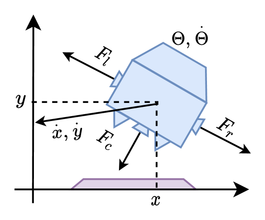
Specifically, the state space has 8 components: horizontal position and velocity (), vertical position and velocity (), angle () and angular momentum (), right and left leg state (that is, leg ground contact). Four different actions can be performed by the agent: no action, fire left engine (), fire right engine () and fire main engine (). The spacecraft has infinite fuel. The reward is computed as follows: -0.3 points for each frame with the main engine on, +100 points for a successful landing, -100 points for crashing, +10 points for each leg making contact with the ground, and a value ranging from 100 to 140 evaluating the spacecraft trajectory to the pad. An episode finishes when the spacecraft lands or crashes. The goal is to land the spacecraft using as less fuel as possible. The environment is considered solved by achieving a cumulative reward of 200 points.
Figure 14 shows the objective value of the hyperparameters optimization process, against the number of trials sampled, for the comparative algorithm. It is worth noting that, actually, good hyperparameters can be found after just 20 trials. It is worth noting that, there is a lower number of trials in the hyperparameters optimization of A2C. Specifically, during the optimization, there are unpromising trials which are aborted during the training process by the pruning algorithm. The figures clearly show that the A2C has been more affected by pruning with respect to the A2CNOG+TE.
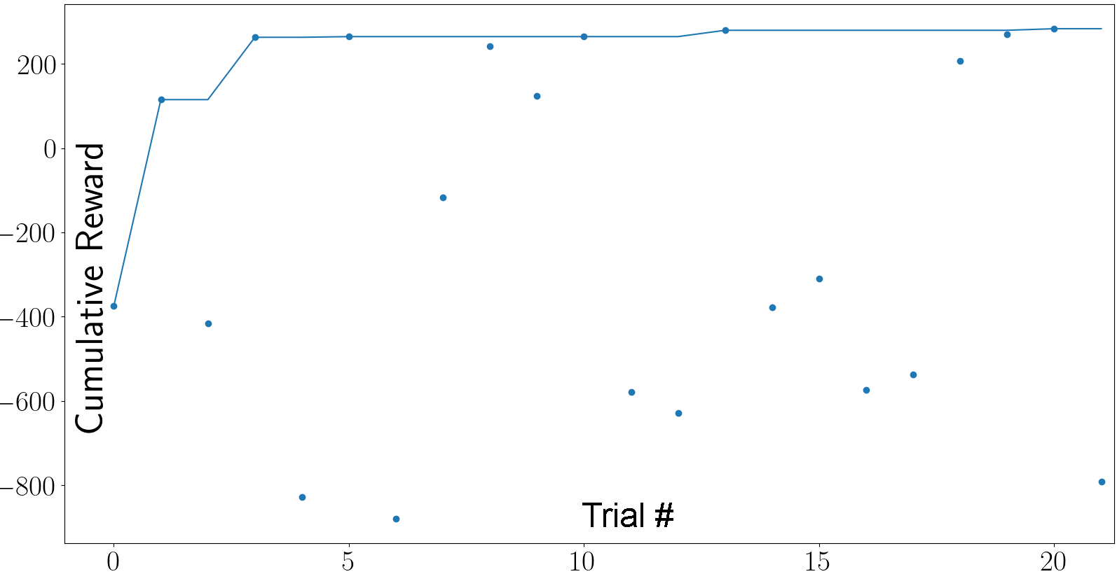
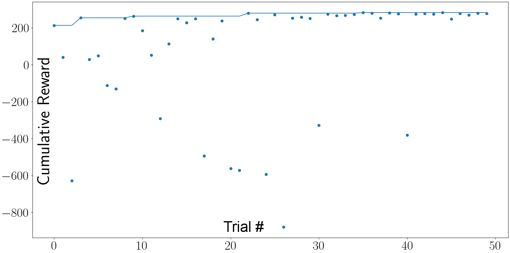
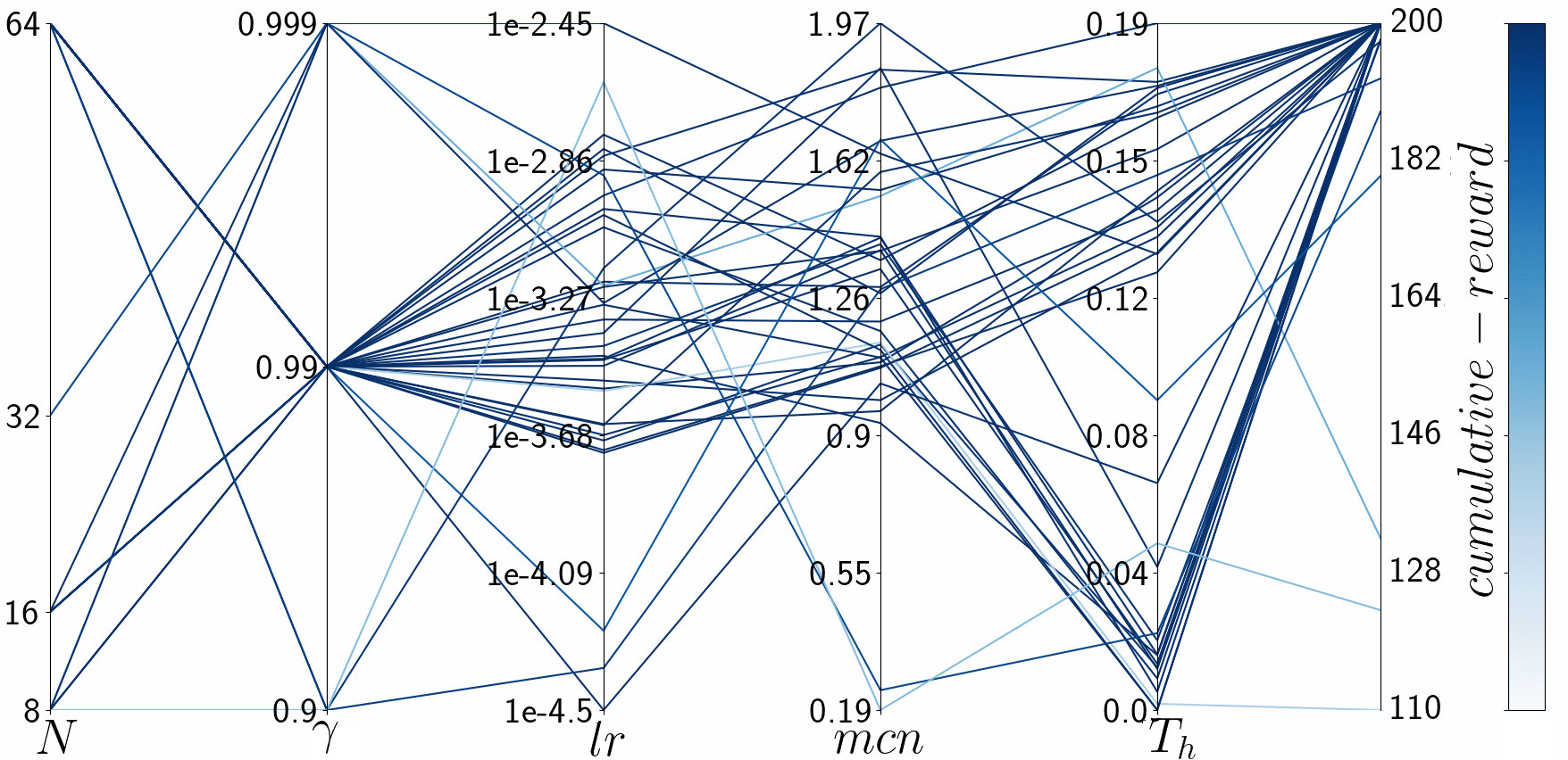
Figure 15 represents the hyperparameters values optimization and the related objective value, for the two algorithms. Here, each line represents a trial, with its hyperparameters values represented on the vertical axes. According to the colorbar, the blue level of the line allows to distinguish the best solutions. In particular, in Figure 15b it can be observed that for some hyperparameters values there is a higher density of good trials.
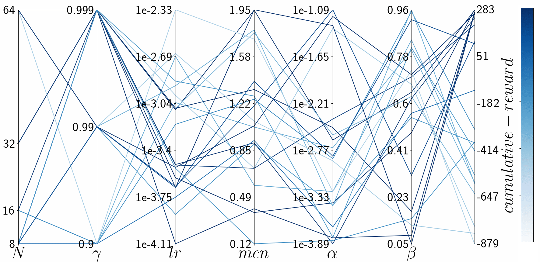
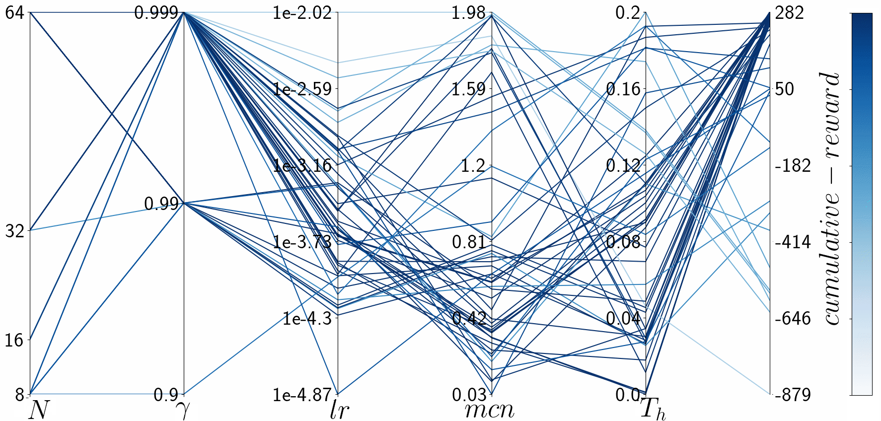
Table 4 shows the best hyperparameters value for each considered algorithm.
| parameter | A2C | A2CNOG+TE |
| 0.999 | 0.999 | |
| 64 | 64 | |
| lr | 0.0002473 | 0.0002292 |
| max-clip-norm | 0.3668 | 0.3462 |
| 0.0003978 | ||
| 0.4832 | ||
| 0.0917 |
After setting the best hyperparameters for each algorithm, the training process has been carried out 10 times for each algorithm.
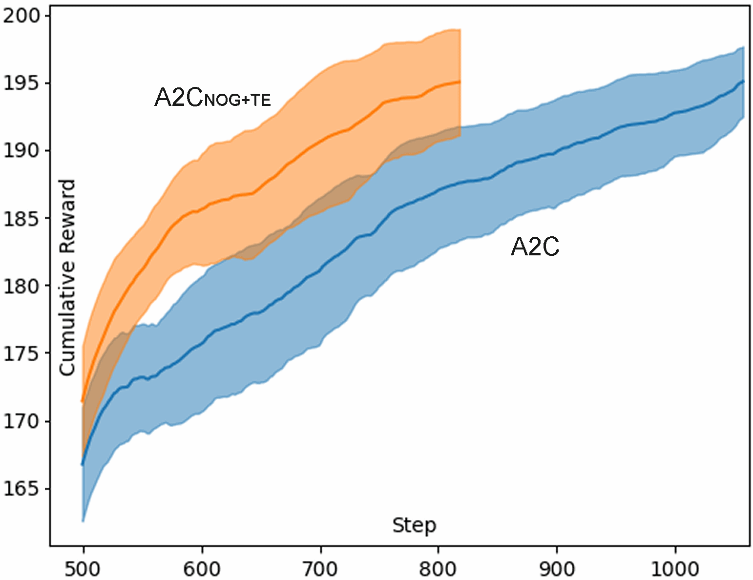
Figure 16 shows the episode reward versus the training step for each algorithm, with its confidence interval. Precisely, the steps to solve the problem via the proposed A2CNOG+TE algorithm and via the classical A2C are and , respectively. It is apparent that the proposed approach sensibly improves the time efficiency of the A2C, up to more than 3.06x of average speedup.
4.5 Results summary
Table 5 summarizes the confidence intervals of the training steps needed to solve the three considered environments, via A2C and A2CNOG+TE, and the speedups with respect to A2C. The effectiveness of the proposed A2CNOG+TE is apparent for increasing environment complexity (i.e., state space size).
| Environment | State space size | A2C | A2CNOG+TE | Average Speedup |
| EnergyMountainCar | 2 | x | ||
| CartPole | 4 | x | ||
| LunarLander | 8 | x |
The A2CNOG+TE algorithm has been developed, tested and publicly released on the Github platform [11], to foster its application on various research environments.
5 Conclusions
In the Advantage Actor Critic (A2C) algorithm, two issues of the scalarization of the multi-objective optimization problem are discussed and addressed. Specifically, an approach to avoid gradient overlapping (NOG) and to control the entropy (TE) of the action distribution is formally designed. The proposed variant, called A2CNOG+TE, and the classical A2C, are experimented, after performing the hyperparameters optimization.
The proposed techniques are designed to be used on all the reinforcement learning algorithms derived from A2C that share the same loss function components. Although the preliminary experiments look promising, more research is needed to both investigate the performance improvements on different environments and on different Advantage based algorithms.
Acknowledgements
This research was partially carried out in the framework of the following projects: (i) PRA 2018_81 project entitled “Wearable sensor systems: personalized analysis and data security in healthcare” funded by the University of Pisa; (ii) CrossLab project (Departments of Excellence), funded by the Italian Ministry of Education and Research (MIUR); (iii) “KiFoot: Sensorized footwear for gait analysis” project, co-funded by the Tuscany Region (Italy) under the PAR FAS 2007-2013 fund and the FAR fund of the Ministry of Education, University and Research (MIUR).
References
- [1] K. Arulkumaran, M. P. Deisenroth, M. Brundage, and A. A. Bharath, “Deep reinforcement learning: A brief survey,” IEEE Signal Processing Magazine, vol. 34, no. 6, pp. 26–38, 2017.
- [2] T. T. Nguyen, “A multi-objective deep reinforcement learning framework,” arXiv preprint arXiv:1803.02965, 2018.
- [3] R. Yang, X. Sun, and K. Narasimhan, “A generalized algorithm for multi-objective reinforcement learning and policy adaptation,” in Advances in Neural Information Processing Systems, pp. 14610–14621, 2019.
- [4] Y. Wu, E. Mansimov, R. B. Grosse, S. Liao, and J. Ba, “Scalable trust-region method for deep reinforcement learning using kronecker-factored approximation,” in Advances in neural information processing systems, pp. 5279–5288, 2017.
- [5] I. Grondman, L. Busoniu, G. A. Lopes, and R. Babuska, “A survey of actor-critic reinforcement learning: Standard and natural policy gradients,” IEEE Transactions on Systems, Man, and Cybernetics, Part C (Applications and Reviews), vol. 42, no. 6, pp. 1291–1307, 2012.
- [6] V. Mnih, A. P. Badia, M. Mirza, A. Graves, T. Lillicrap, T. Harley, D. Silver, and K. Kavukcuoglu, “Asynchronous methods for deep reinforcement learning,” in International conference on machine learning, pp. 1928–1937, 2016.
- [7] J. S. Bergstra, R. Bardenet, Y. Bengio, and B. Kégl, “Algorithms for hyper-parameter optimization,” in Advances in neural information processing systems, pp. 2546–2554, 2011.
- [8] M. Tokic and G. Palm, “Gradient algorithms for exploration/exploitation trade-offs: Global and local variants,” in Artificial Neural Networks in Pattern Recognition (N. Mana, F. Schwenker, and E. Trentin, eds.), (Berlin, Heidelberg), pp. 60–71, Springer Berlin Heidelberg, 2012.
- [9] G. Brockman, V. Cheung, L. Pettersson, J. Schneider, J. Schulman, J. Tang, and W. Zaremba, “Openai gym,” 2016.
- [10] L. Li, K. G. Jamieson, A. Rostamizadeh, E. Gonina, M. Hardt, B. Recht, and A. Talwalkar, “A system for massively parallel hyperparameter tuning,” CoRR, vol. abs/1810.05934, 2018.
- [11] F. A. Galatolo, “https://github.com/galatolofederico/a2c-te-nog,” 2020.
Authors
- Federico A. Galatolo
-
is a PhD student in Information Engineering at the Department of Information Engineering of the University of Pisa (Italy). His research is focused on Computational Stigmergy, Deep Learning and Reinforcement Learning.
- Mario G.C.A. Cimino
-
is an associate professor at the Department of Information Engineering of the University of Pisa (Italy). His research lies in the areas of Information Systems and Artificial intelligence. He is (co-) author of about 70 scientific publications.
- Gigliola Vaglini
-
is full professor of Computer Engineering at “Dipartimento di Ingegneria della Informazione” of the University of Pisa. The main fields of her research activity are the specification and verification of concurrent and distributed systems, and the use of machine learning techniques for detecting malware in mobile systems and anomalies of industrial systems.