Vol.0 (20xx) No.0, 000–000
22institutetext: Southern African Large Telescope, P.O. Box 9, Observatory, Cape Town, 7935 South Africa
33institutetext: Sternberg Astronomical Institute, Lomonosov Moscow State University, Moscow, 119992 Russia
44institutetext: Institute of Astronomy of RAS, Moscow, Russia
55institutetext: New York University Abu Dhabi, PO Box 129188, Abu Dhabi, UAE
66institutetext: Center for Astro, Particle, and Planetary Physics, NYU Abu Dhabi, PO Box 129188, Abu Dhabi, UAE
\vs\noReceived 20xx month day; accepted 20xx month day
Long-period eclipsing binaries: towards the true mass-luminosity relation. I. The test sample, observations and data analysis.
Abstract
The mass-luminosity relation is a fundamental law of astrophysics. We have suggested that the currently used mass-luminosity relation is not correct for the range of mass since it was created using double-lined eclipsing binaries, where the components are synchronized and consequently change each other’s evolutionary path. To exclude this effect we have started a project to study long-period massive eclipsing binaries in order to construct radial velocity curves and determine masses for the components. We outline our project and present the selected test sample together with the first HRS/SALT spectral observations and the software package, fbs (Fitting Binary Stars), that we developed for the analysis of our spectral data. As the first result we present the radial velocity curves and best-fit orbital elements for the two components of the FP Car binary system from our test sample.
keywords:
stars: luminosity function, mass function — stars: binaries: spectroscopic1 Introduction
The mass of a star is the parameter that, to a first approximation, is most important in determining its evolution. However, the mass cannot be dynamically determined for a single star, so indirect methods have been developed for estimating stellar masses. The most widely used of them is to estimate the mass from observations of the distribution of another parameter for a stellar ensemble under study (field stars, cluster stars). The stellar luminosity is the most commonly used parameter, and the subsequent transition to masses of stars is made using the so-called mass-luminosity relation (MLR).
Independent determination of the mass of a star and its luminosity is only possible for components of binary systems of certain types.
One suitable type of binary system is a visual binary star with known orbital parameters and trigonometric parallax. Such stars are usually wide pairs, whose components do not interact with each other and are evolutionarily similar to single stars. In addition, usually they are in the nearest solar neighborhood and, therefore, are mostly low-mass stars. The problem of determining the masses of visual binaries was discussed, for example, in Docobo et al. (2016); Malkov et al. (2012); Fernandes et al. (1998). The construction of the MLR for low-mass stars based on observational data is discussed in Henry (2004); Delfosse et al. (2000); Henry et al. (1999); Malkov et al. (1997).
Another major source of independently defined stellar masses is detached eclipsing binary stars with components on the main sequence, where the spectral lines of both components are observed (hereafter double-lined eclipsing binaries, DLEB). These stars are usually relatively massive () and their parameters are used to construct the stellar MLR for intermediate and large masses. The exact parameters of DLEB stars and the MLR based on them can be found, for example, in Torres et al. (2010); Kovaleva (2001); Gorda & Svechnikov (1998); Andersen (1991); Popper (1980).
When these two MLRs (based on the visual binaries and on the DLEB stars with components on the main sequence) are jointly analyzed and used (in particular, in order to compare the theoretical MLRs with empirical data), it is generally assumed by default, that the components of the detached close binaries and the wide binaries evolve in a similar way. It should be noted, however, that DLEB are close pairs whose components’ rotation is synchronized by tidal interaction, and, due to rotational deceleration, they evolve differently than “isolated” (i.e., single or wide binary systems) stars.
When comparing the radii of DLEB and single stars (Malkov 2003), a noticeable difference between the observed parameters of B0V–G0V components of DLEB and of single stars of similar spectral classes was found. This difference was confirmed by analysis of independent studies published by other authors. This difference also explains the disagreement between the published scales of bolometric corrections. Larger radii and higher temperatures of A-F components of DLEB stars can be explained by the synchronization and associated slowing down of rotation of such components in close systems. Another possible reason is the effect of observational selection: due to the non-sphericity of the rotating stars, the parameters determined from the observations depend on the relative orientations of their rotation axes. Isolated stars are oriented randomly, while components of eclipsing binaries are usually observed from near the equatorial plane. Systematically smaller observed radii of DLEB stars of spectral class B can be explained by the fact that stars with large radii do not occur with companions on the main sequence: most of them have already filled their Roche lobe (which stopped their further growth) and have become semi-detached systems (which excluded them from the discussed statistics). Then, in Malkov (2007) data for the fundamental parameters of the components of a few currently known long-period DLEB have been collected. These stars presumably have not undergone synchronization of rotation with the orbital period and therefore spin rapidly, and evolve similarly to single stars.
The theory of synchronization (and circularization) in close binary systems developed by Zahn (1975, 1977) is based on the mechanism of energy dissipation via dynamic tides in non-adiabatic surface layers of the component stars. Another theory was developed by Tassoul (1987, 1988), and is based on tidal dissipation of the kinetic energy of large-scale meridional flows. In their critical reviews, Khaliullin & Khaliullina (2007, 2010) point out that both the circularization and synchronization time-scales implied by these mechanisms differ by almost three orders of magnitude, and, based on an analysis of the observed rates of apsidal motion, show that the observed synchronization times agree with Zahn’s theory but are inconsistent with the shorter time-scale proposed by Tassoul.
The synchronization time depends primarily on the stellar mass and the binary separation. So, for example, according to Tassoul (1987), the synchronization time for orbital periods up to about 25 days is smaller than one-tenth of the main-sequence life-time of a star.
The theories of synchronization mentioned above have been developed for early-type, massive stars with radiative envelopes (i.e., for stars with ). In the current work, to construct the mass-luminosity relation for “isolated” stars, we study DLEB stars in the range , as the masses of components of other types of binary stars (visual binaries, resolved spectroscopic binaries) rarely exceed this limit (stars in the range will be considered later). According to the shorter time-scale theory of Tassoul, the synchronization time becomes comparable to the main-sequence life-time of a star for orbital periods of the order of 50-70 days (the longer time-scale theory of Zahn predicts even shorter periods).
Currently there is no way to properly estimate the degree to which the effect on the IMF may be important for , as available observational data for that mass range are too poor to draw definite conclusions. For that reason we have started a pilot project to study long-period massive eclipsing binaries to construct radial velocity curves and determine the masses of their components. Using published photometric data or light-curve solutions we expect to obtain luminosities for the individual components. With accurate luminosity determinations we plan to compare their location on the mass-luminosity diagram with the “standard” MLR. As a result of this pilot study we plan to confirm that rapid and slow rotators satisfy different MLRs, which should be used for different purposes. Then the feasibility of a larger project, the construction of a reliable “fast rotators” MLR, will be considered. The data we obtain will also be used to establish mass-radius and mass-temperature relations.
2 The Test Sample, Observations and Data reduction
| # | Name | RA (2000.0) | DEC (2000.0) | mag | e | Period |
|---|---|---|---|---|---|---|
| (1) | (2) | (3) | (4) | (5) | (6) | (7) |
| 01 | V883 Ara | 16:51:45.10 | -50:17:46.5 | 8.55 | 0 | 61.8740 |
| 02 | KV CMa | 06:50:52.67 | -20:54:37.4 | 7.16 | 0 | 68.3842 |
| 03 | V338 Car | 11:13:52.31 | -58:36:30.4 | 9.30 | 0 | 74.6429 |
| 04 | V884 Mon | 07:05:11.84 | -11:06:02.4 | 9.13 | 0 | 123.2100 |
| 05 | V766 Sgr | 17:51:57.00 | -28:17:02.0 | 10.80 | 0 | 147.1050 |
| 06 | FP Car | 11:04:35.87 | -62:34:22.2 | 9.70 | 0 | 176.0270 |
| 07 | V1108 Sgr | 19:12:43.63 | -18:08:12.0 | 11.50 | 0 | 46.5816 |
| 08 | PW Pup | 07:49:06.00 | -31:07:42.6 | 9.20 | 0 | 158.0000 |
| 09 | mu Sgr | 18:13:45.81 | -21:03:31.8 | 3.80 | 0 | 180.5500 |
| 10 | AL Vel | 08:31:11.28 | -47:39:57.4 | 8.60 | 0 | 96.1070 |
| 11 | NN Del | 20:46:49.22 | +07:33:10.4 | 8.39 | 0 | 99.2684 |
To compile the test sample for our pilot project we used the Catalog of Eclipsing Variables (hereafter CEV; Malkov et al. 2007; Avvakumova et al. 2013; Avvakumova & Malkov 2014) from which we have carefully selected 11 massive long-period (i.e., presumably non-synchronised) detached main-sequence eclipsing systems that are presented in Table 1. The selected systems should have components of similar luminosities (i.e., can be observed as SB2 systems – spectroscopic binaries, where spectral lines from both components are visible) and guarantee an accurate determination of stellar parameters (in particular masses to 3%) of early-type stars composing them. We planned to obtain a minimum of five spectra for targets with circular orbits () and a minimum of 10 spectra for targets with non-circular orbits (). This number of spectra should be enough to find a credible orbital solution and to complete the science objectives.
All observations were obtained with the High Resolution Spectrograph (HRS; Barnes et al. 2008; Bramall et al. 2010, 2012; Crause et al. 2014) at the Southern African Large Telescope (SALT; Buckley et al. 2006; O’Donoghue et al. 2006). The HRS was used in the medium resolution (MR) mode, that gives a spectral resolution R36 500–39 000; it has an input fiber diameter of 2.23 arcsec for both object and sky. All our échelle data were obtained during 2017–2019 and cover the total spectral range 3900–8900 Å, where both blue and red CCDs were used with 11 binning. All science observations were supported by the HRS Calibration Plan, which includes a set of bias frames at the beginning of each observational night and a set of flat-fields and a spectrum of a ThAr lamp once per week. Since the HRS is a vacuum échelle spectrograph installed inside a temperature-controlled enclosure such a set of calibrations is enough to give an average external velocity accuracy of 300 m s-1 (Kniazev et al. 2019). HRS data underwent a primary reduction with the SALT science pipeline (Crawford et al. 2010), which includes overscan correction, bias subtractions and gain correction. After that échelle spectroscopic reduction was carried out using the HRS pipeline described in detail in Kniazev et al. (2016, 2019).
3 Fitting Binary Stars: full pixel fitting method
To analyze fully reduced HRS spectra of binary systems and to determine stellar atmosphere parameters for each component such as effective temperature , surface gravity , metallicity [Z/H] as well as stellar rotation and line-of-sight velocities we developed a dedicated Python-based package, Fitting Binary Stars (fbs) (Katkov et al., 2020 in preparation). The fbs implements a full pixel fitting approach to simultaneous approximation of multiple epoch spectra of binary system by combination of two synthetic stellar models using minimization. The fbs developed on top of the non-linear minimization lmfit package (Newville et al. 2016) provides a high-level interface to many optimization methods (e.g. Levenberg-Marquardt, Powell, Downhill simplex Nelder-Mead method, Differential evolution etc.).
During the evaluation of the fbs proceeds by the following steps: First, the fbs interpolates two stellar templates from the grid of synthetic stellar spectra for given sets of stellar atmosphere parameters (Teff, , [Z/H])1,2. The interpolation has to be fast to work with high-resolution stellar spectra containing tens to hundreds thousands of pixels in the spectral range under analysis. Therefore, we propose an algorithm where the fbs pre-calculates the Delaunay triangulation in 3 dimensions of stellar model parameters (, , [Z/H]) using nodes of the synthetic grid. Interpolating the fbs finds the simplex containing the given point, then averages the spectra from the simplex vertices with weights inversely proportional to the squared distance to the vertex. Such an algorithm is very fast and might work on regular as well as irregular model grids with missing nodes. Then, the model templates are broadened by individual stellar rotation 1,2 and shifted for the line-of-sight velocities , at the epoch of the -th spectrum. The last two steps are to sum templates with weights and multiply the spectrum by the extinction curve appropriate to ithe assumed or to multiply the final spectrum by a polynomial continuum to match the difference between the observed and synthetic spectra. In such an approach the value can be written as follows:
| (1) |
| (2) |
where , , represent the observed spectrum at the -th epoch, its uncertainties and the model, respectively; is the stellar template interpolated from the grid of stellar models; is the convolution kernel to derive the broadening effect due to stellar rotation (Gray 1992) and to shift the templates by the line-of-sight velocity of each binary star component at epoch ; “” denotes convolution; is a polynomial multiplicative continuum or extinction curve for the given . The approach produces the following parameters: , , [Z/H], for both components of the binary star, pairs of line-of-sight radial velocities , for spectra observed at different epochs and for the system.
Hereafter, we usualy employ Coelho (2014) stellar models (stars with T K), which match the HRS MR instrumental resolution (Kniazev et al. 2019) well. Also we adapted high-resolution tlusty models (T K; Lanz & Hubeny 2003, 2007) and phoenix models (T K; Husser et al. 2013), convolving them to match the HRS MR instrumental resolution.
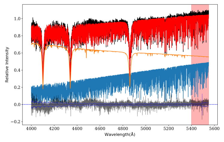
Due to the extensive functionality of the lmfit package, the fbs provides flexible control over model parameters, including upper/lower bounding, parameter fixing and making parameters connected. As an example, connecting stellar component metallicities () might be a reasonable approximation for binary stars formed in the same gas cloud. An example of the use of the fbs software is shown in Figure 2 for three spectra of the binary system FP Car from our test sample. The fbs is a full pixel fitting approach and allows us to approximate the full spectral range of the given spectrum or one or several spectral intervals as well as to easily mask bad pixels and/or spectral regions. The fbs also contains basic functionality to determine orbital parameters from the stellar rotation curves.

4 Check-up of the External Accuracy
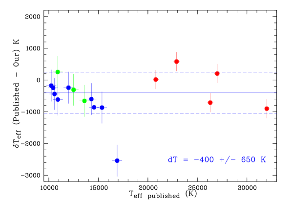
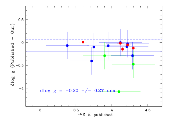
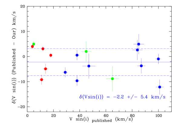
To check the external accuracy of our fbs software, we make different tests. For one of them we fitted with fbs program 18 echelle spectra of early and late B-type stars, that were obtained with the Fibre-fed Extended Range Optical Spectrograph (FEROS; Kaufer et al. 1996) and were modelled and published (Hempel & Holweger 2003; Nieva & Przybilla 2012; Bailey & Landstreet 2013). For this fit we used models from Coelho (2014) for the late B-stars and models from Lanz & Hubeny (2003, 2007) for the early B-stars. The comparison of our results for , and with results published earlier are shown in Figure 2. Our found is comparable to the previously found with rms of 650 K, with rms of 0.27 dex and with rms of 5.4 km s-1 that are very close to cited errors that are shown with gorizontal bars. There are no any obvious systematic issues are visible in this Figure.
| Parameter | Value | % |
|---|---|---|
| Epoch at radial velocity maximum (d) | 0.00 | |
| Orbital period (d) | 176.0320.010 | 0.00 |
| Eccentricity | 0 (fixed) | 0.00 |
| Radial velocity semi-amplitude (km s-1) | 22.920.73 | 3.20 |
| Radial velocity semi-amplitude (km s-1) | 35.300.26 | 0.72 |
| Systemic heliocentric velocity (km s-1) | 15.310.15 | 0.96 |
| Root-mean-square residuals of Keplerian fit (km s-1) | 0.976 | – |
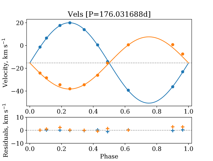
5 First Results: the FP Car system
As the first result we would like to present here some our results on the study of the FP Car binary system that belongs to our test sample (see Table 1). FP Car (HD96214) as a variable star with period of 176 days was discovered by Cannon (1926). The period of this system was measured more accurate by Dvorak (2004) using data from ASAS survey (Pojmanski 1997). The spectral type was estimated by Houk & Cowley (1975) as B5/7(V). Approximate masses and for both components were calculated by Brancewicz & Dworak (1980) with use their iterative method for computation of geometric and physical parameters for components of eclipsing binary stars.
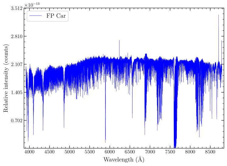
Our spectral observations of FP Car were made during 2017–2019 with HRS at SALT (see Section 2). Ten spectra were obtained in total covering all phases of the binary’s orbit. After the standard HRS reduction, additionally, each HRS spectrum of FP Car was corrected for bad columns and pixels and was also corrected for the spectral sensitivity curve obtained closest to the date of the observation. Spectrophotometric standards for HRS were observed once a week as a part of the HRS Calibration Plan. Figure 3 presents one of a fully processed spectrum of FP Car, which was used in further analysis. The spectrum consists of 70 échelle orders from both the blue and the red arms of HRS merged together and corrected for sensitivity. Unfortunately, SALT is a telescope where the unfilled entrance pupil of the telescope moves during the observation and for that reason the absolute flux calibration is not feasible with SALT. At the same time, since all optical elements are always the same, the relative flux calibration can be used for SALT data.
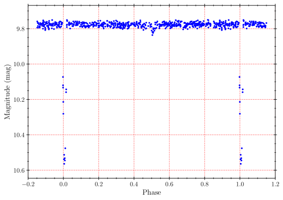
All HRS observations of the FP Car system were used simultaneously for the calculation of radial velocity curves using fbs package. The determination of orbital parameters from the stellar rotation curves was also done with fbs package as it is shown in Figure 5 and presented in Table 2. The found period is P=176.0320.010 days that is in agreement within uncertainties with photometric period presented in Table 1. Our spectral data show that system has circular orbit (e=0) and this parameter was fixed for the last iteration. Our found amplitudes of velocities have small errors 0.7% for the component B (blue) and 3.2% for the component A (orange) that is totally in agreement with fit shown in Figure 2, where spectrum of the component B shows many narrow lines and spectrum of the component A shows only wide Balmer and helium lines with km s-1. Finally, we can calculate masses of both components for the FP Car system as and , where is the orbital inclination angle that can only be determined from the modeling of photometric data. Unfortunately, there is no good photometric data for FP Car among all existing public surveys. The best available data are from the ASAS survey (Pojmanski 1997) as shown in Figure 6. However, even these data have too few points outlining the positions and shapes of the narrow primary and secondary minima and it is impossible to use these data for any modeling. For that reason we are actively accumulating photometric data for FP Car and other stars from our test sample using the telescope network LCO (Brown et al. 2013).
6 Conclusions
We present our new project on study of the long-period massive eclipsing binaries, where components are not synchronized and for this reason not changed the evolution scenario of each other. Small sample of eleven binary systems was described here that was formed for the pilot spectroscopy with HRS/SALT. The software package fbs (Fitting Binary Stars) was developed by us for the analysis of spectral data. We describe this package and show its external accuracy in determination stellar parameters. As the first result we present the radial velocity curves and the best-fit orbital elements for both components of the FP Car binary system from our test sample.
Acknowledgements.
All spectral observations reported in this paper were obtained with the Southern African Large Telescope (SALT) under programs 2016-1-MLT-002, 2017-1-MLT-001 and 2019-1-SCI-004 (PI: Alexei Kniazev). AK acknowledges support from the National Research Foundation of South Africa. OM acknowledges support by the Russian Foundation for Basic Researches grant 20-52-53009. IK acknowledges support by the Russian Science Foundation grant 17-72-20119. LB acknowledges support by the Russian Science Foundation grants 18-02-00890 and 19-02-00611.References
- Andersen (1991) Andersen, J. 1991, A&A Rev., 3, 91
- Avvakumova & Malkov (2014) Avvakumova, E. A., & Malkov, O. Y. 2014, MNRAS, 444, 1982
- Avvakumova et al. (2013) Avvakumova, E. A., Malkov, O. Y., & Kniazev, A. Y. 2013, Astronomische Nachrichten, 334, 860
- Bailey & Landstreet (2013) Bailey, J. D., & Landstreet, J. D. 2013, A&A, 551, A30
- Barnes et al. (2008) Barnes, S. I., Cottrell, P. L., Albrow, M. D., et al. 2008, Society of Photo-Optical Instrumentation Engineers (SPIE) Conference Series, Vol. 7014, The optical design of the Southern African Large Telescope high resolution spectrograph: SALT HRS, Society of Photo-Optical Instrumentation Engineers (SPIE) Conference Series, Vol. 7014, Ground-based and Airborne Instrumentation for Astronomy II. Edited by McLean, Ian S.; Casali, Mark M. Proceedings of the SPIE, Volume 7014, article id. 70140K, 12 pp. (2008)., 70140K
- Bramall et al. (2010) Bramall, D. G., Sharples, R., Tyas, L., et al. 2010, Society of Photo-Optical Instrumentation Engineers (SPIE) Conference Series, Vol. 7735, The SALT HRS spectrograph: final design, instrument capabilities, and operational modes, Society of Photo-Optical Instrumentation Engineers (SPIE) Conference Series, Vol. 7735, Proceedings of the SPIE, Volume 7735, id. 77354F (2010)., 77354F
- Bramall et al. (2012) Bramall, D. G., Schmoll, J., Tyas, L. M. G., et al. 2012, Society of Photo-Optical Instrumentation Engineers (SPIE) Conference Series, Vol. 8446, The SALT HRS spectrograph: instrument integration and laboratory test results, Society of Photo-Optical Instrumentation Engineers (SPIE) Conference Series, Vol. 8446, Ground-based and Airborne Instrumentation for Astronomy IV. Proceedings of the SPIE, Volume 8446, article id. 84460A, 9 pp. (2012)., 84460A
- Brancewicz & Dworak (1980) Brancewicz, H. K., & Dworak, T. Z. 1980, Acta Astron., 30, 501
- Brown et al. (2013) Brown, T. M., Baliber, N., Bianco, F. B., et al. 2013, PASP, 125, 1031
- Buckley et al. (2006) Buckley, D. A. H., Swart, G. P., & Meiring, J. G. 2006, Society of Photo-Optical Instrumentation Engineers (SPIE) Conference Series, Vol. 6267, Completion and commissioning of the Southern African Large Telescope, Society of Photo-Optical Instrumentation Engineers (SPIE) Conference Series, Vol. 6267, Ground-based and Airborne Telescopes. Edited by Stepp, Larry M.. Proceedings of the SPIE, Volume 6267, id. 62670Z (2006)., 62670Z
- Cannon (1926) Cannon, A. J. 1926, Harvard College Observatory Bulletin, 837, 1
- Coelho (2014) Coelho, P. R. T. 2014, MNRAS, 440, 1027
- Crause et al. (2014) Crause, L. A., Sharples, R. M., Bramall, D. G., et al. 2014, Society of Photo-Optical Instrumentation Engineers (SPIE) Conference Series, Vol. 9147, Performance of the Southern African Large Telescope (SALT) High Resolution Spectrograph (HRS), Society of Photo-Optical Instrumentation Engineers (SPIE) Conference Series, Vol. 9147, Proceedings of the SPIE, Volume 9147, id. 91476T 14 pp. (2014)., 91476T
- Crawford et al. (2010) Crawford, S. M., Still, M., Schellart, P., et al. 2010, Society of Photo-Optical Instrumentation Engineers (SPIE) Conference Series, Vol. 7737, PySALT: the SALT science pipeline, Society of Photo-Optical Instrumentation Engineers (SPIE) Conference Series, Vol. 7737, Proceedings of the SPIE, Volume 7737, id. 773725 (2010)., 773725
- Delfosse et al. (2000) Delfosse, X., Forveille, T., Ségransan, D., et al. 2000, A&A, 364, 217
- Docobo et al. (2016) Docobo, J. A., Tamazian, V. S., Malkov, O. Y., Campo, P. P., & Chulkov, D. A. 2016, MNRAS, 459, 1580
- Dvorak (2004) Dvorak, S. W. 2004, Information Bulletin on Variable Stars, 5542, 1
- Fernandes et al. (1998) Fernandes, J., Lebreton, Y., Baglin, A., & Morel, P. 1998, A&A, 338, 455
- Gorda & Svechnikov (1998) Gorda, S. Y., & Svechnikov, M. A. 1998, Astronomy Reports, 42, 793
- Gray (1992) Gray, D. F. 1992, The observation and analysis of stellar photospheres., Vol. 20
- Hempel & Holweger (2003) Hempel, M., & Holweger, H. 2003, A&A, 408, 1065
- Henry (2004) Henry, T. J. 2004, in Astronomical Society of the Pacific Conference Series, Vol. 318, Spectroscopically and Spatially Resolving the Components of the Close Binary Stars, ed. R. W. Hilditch, H. Hensberge, & K. Pavlovski, 159
- Henry et al. (1999) Henry, T. J., Franz, O. G., Wasserman, L. H., et al. 1999, ApJ, 512, 864
- Houk & Cowley (1975) Houk, N., & Cowley, A. P. 1975, University of Michigan Catalogue of two-dimensional spectral types for the HD stars. Volume I. Declinations -90. to -53.
- Husser et al. (2013) Husser, T. O., Wende-von Berg, S., Dreizler, S., et al. 2013, A&A, 553, A6
- Kaufer et al. (1996) Kaufer, A., Stahl, O., Wolf, B., et al. 1996, A&A, 305, 887
- Khaliullin & Khaliullina (2007) Khaliullin, K. F., & Khaliullina, A. I. 2007, MNRAS, 382, 356
- Khaliullin & Khaliullina (2010) Khaliullin, K. F., & Khaliullina, A. I. 2010, MNRAS, 401, 257
- Kniazev et al. (2016) Kniazev, A. Y., Gvaramadze, V. V., & Berdnikov, L. N. 2016, MNRAS, 459, 3068
- Kniazev et al. (2019) Kniazev, A. Y., Usenko, I. A., Kovtyukh, V. V., & Berdnikov, L. N. 2019, Astrophysical Bulletin, 74, 208
- Kovaleva (2001) Kovaleva, D. A. 2001, Astronomy Reports, 45, 972
- Lanz & Hubeny (2003) Lanz, T., & Hubeny, I. 2003, ApJS, 146, 417
- Lanz & Hubeny (2007) Lanz, T., & Hubeny, I. 2007, ApJS, 169, 83
- Malkov (2003) Malkov, O. Y. 2003, A&A, 402, 1055
- Malkov (2007) Malkov, O. Y. 2007, MNRAS, 382, 1073
- Malkov et al. (2007) Malkov, O. Y., Oblak, E., Avvakumova, E. A., & Torra, J. 2007, A&A, 465, 549
- Malkov et al. (1997) Malkov, O. Y., Piskunov, A. E., & Shpil’Kina, D. A. 1997, A&A, 320, 79
- Malkov et al. (2012) Malkov, O. Y., Tamazian, V. S., Docobo, J. A., & Chulkov, D. A. 2012, A&A, 546, A69
- Newville et al. (2016) Newville, M., Stensitzki, T., Allen, D. B., et al. 2016, Lmfit: Non-Linear Least-Square Minimization and Curve-Fitting for Python
- Nieva & Przybilla (2012) Nieva, M. F., & Przybilla, N. 2012, A&A, 539, A143
- O’Donoghue et al. (2006) O’Donoghue, D., Buckley, D. A. H., Balona, L. A., et al. 2006, MNRAS, 372, 151
- Pojmanski (1997) Pojmanski, G. 1997, Acta Astron., 47, 467
- Popper (1980) Popper, D. M. 1980, ARA&A, 18, 115
- Tassoul (1987) Tassoul, J.-L. 1987, ApJ, 322, 856
- Tassoul (1988) Tassoul, J.-L. 1988, ApJ, 324, L71
- Torres et al. (2010) Torres, G., Andersen, J., & Giménez, A. 2010, A&A Rev., 18, 67
- Zahn (1975) Zahn, J. P. 1975, A&A, 41, 329
- Zahn (1977) Zahn, J. P. 1977, A&A, 500, 121