LBsoft: a parallel open-source software for simulation of colloidal systems

Abstract

We present LBsoft, an open-source software developed mainly to simulate the hydro-dynamics of colloidal systems based on the concurrent coupling between lattice Boltzmann methods for the fluid and discrete particle dynamics for the colloids. Such coupling has been developed before, but, to the best of our knowledge, no detailed discussion of the programming issues to be faced in order to attain efficient implementation on parallel architectures, has ever been presented to date. In this paper, we describe in detail the underlying multi-scale models, their coupling procedure, along side with a description of the relevant input variables, to facilitate third-parties usage.

The code is designed to exploit parallel computing platforms, taking advantage also of the recent AVX-512 instruction set. We focus on LBsoft structure, functionality, parallel implementation, performance and availability, so as to facilitate the access to this computational tool to the research community in the field.

The capabilities of LBsoft are highlighted for a number of prototypical case studies, such as pickering emulsions, bicontinuous systems, as well as an original study of the coarsening process in confined bijels under shear.

PROGRAM SUMMARY

Program Title: LBsoft
Licensing provisions: 3-Clause BSD License
Programming language: Fortran 95
Nature of problem: Hydro-dynamics of the colloidal multi-component systems and Pickering emulsions.
Solution method: Numerical solutions to the Navier-Stokes equations by Lattice-Boltzmann (lattice-Bhatnagar-Gross-Krook, LBGK) method [1] describing the fluid dynamics within an Eulerian description. Numerical solutions to the equations of motion describing a set of discrete colloidal particles within a Lagrangian representation coupled to the LBGK solver [2]. The numerical solution of the coupling algorithm includes the back reaction effects for each force terms following a multi-scale paradigm.

[1] S. Succi, The Lattice Boltzmann Equation: For Fluid Dynamics and Beyond, Oxford University Press, 2001.

[2] A. Ladd,R. Verberg, Lattice-Boltzmann simulations of particle-fluid suspensions, J. Stat. Phys. 104.5-6 (2001) 1191-1251

1 Introduction

In the last two decades, the design of novel mesoscale soft materials has gained considerable interest. In particular, soft-glassy materials (SGM) like emulsions, foams and gels have received a growing attention due to their applications in several areas of modern industry. For instance, chemical and food processing, manufacturing and biomedical involve several soft-glassy materials nowadays [1, 2, 3]. Besides their technological importance, the intriguing non-equilibrium effects, such as long-time relaxation, yield-stress behaviour and highly non-Newtonian dynamics make these materials of significant theoretical interest. A reliable model of these features alongside with its software implementation is of compelling interest for the rational designing and shaping up of novel soft porous materials. In this context, computational fluid dynamics (CFD) can play a considerable role in numerical investigations of the underpinning physics in order to enhance mainly mechanical properties, thereby opening new scenarios in the realisation of new states of matter.

Nowadays, the lattice-Boltzmann method (LBM) is one of the most popular techniques for the simulation of fluid dynamics due to its relative simplicity and locality of the underlying algorithm. A straightforward parallelization of the method is one of the main advantages of the lattice-Boltzmann algorithm which makes it an excellent tool for high-performance CFD.

Starting with the LBM development, a considerable effort has been carried out to include the hydrodynamic interactions among solid particles and fluids [4, 5, 6, 7]. This extension has opened the possibility to simulate complex colloidal systems also referred to as Pickering emulsions [8]. In this framework, the description of the colloidal particles exploits a Lagrangian dynamics solver coupled to the lattice-Boltzmann solver of fluid dynamics equations. This intrinsically multiscale approach can catch the dynamical transition from a bi-continuous interfacially jammed emulsion gel to a Pickering emulsion, highlighting the mechanical and spatial properties which are of primary interest for the rational design of SGM [9, 10, 11, 12].

By now, several LBM implementations are available, both academic packages such as OpenLB [13], DL_MESO [14], also implementing particle-fluid interaction such as WaLBerla [15, 16], Palabos [17], Ludwig [18], HemeLB [19], and commercially licensed software such as XFlow [20] and PowerFLOW [21], to name a few. The modelling of SGM requires specific implementations of LBM and Lagrangian solvers aimed at the optimization of the multi-scale coupling algorithms in order to scale up to large systems. This point is mandatory for an accurate statistical description of such complex systems which is necessary for a fully rational design of a new class of porous materials.

In this paper, we present, along with the overall model, LBsoft, a parallel FORTRAN code, specifically designed to simulate bi-continuous systems with colloidal particles under a variety of different conditions. This comprehensive platform is devised in such a way to handle both LBGK solver and particle dynamics via a scalable multiscale algorithm. The framework is developed to exploit several computational architectures and parallel decompositions. With most of the parameters taken from relevant literature in the field, several test cases have been carried out as a software benchmark.

The paper is structured as follows. In Section 2 we report a brief description of the underlying method. A full derivation of the model is not reported, but we limit the presentation to the main ingredients necessary to describe the implementation of the algorithms. Nonetheless, original references of models are reported step by step along with the implementation description. In Section 3 we describe the details on memory organisation and parallel communication patterns. In Section 4 we report a set of tests used to validate the implementation and assess the parallel performance. Finally, conclusions and an outlook on future development directions are presented.

2 Method

In this section, we briefly review the methodology implemented in LBsoft. Further details are available in the literature.

The code combines two different levels of description: the first exploits a continuum description for the hydrodynamics of a single or two immiscible fluids; the second utilises individual rigid bodies for the representation of colloidal particles or other suspended species. The exchange of information between the two levels is computed on-the-fly, allowing a simultaneous evolution in time of both fluids and particles.

2.1 Single component lattice-Boltzmann

The lattice-Boltzmann equation facilitates the simulation of flows and hydrodynamic interactions in fluids by a fully discretised analogue of the Boltzmann kinetic equation. In the LBM approach, the fundamental quantity is $f_{i}(\vec{r};t)$, namely the probability of finding a “fluid particle” at the spatial mesh point $\vec{r}$ and at time $t$ with velocity $c_{i}$ selected from a finite set of possible speeds. The LBsoft code implements the three-dimensional 19-speed cubic lattice (D3Q19) with the discrete velocities $c_{i}$ ($i\in[0,...,18]$) connecting mesh points with spacing $\Delta x$ , located at distance $1\Delta x$ and $\sqrt{2}\Delta x$, first and second neighbors, respectively (see Fig. 1).

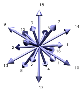
Figure 1: The set of discrete velocities for the three-dimensional 19-speed cubic lattice (D3Q19).

Denoted $\rho(\vec{r};t)$ and $\vec{u}(\vec{r};t)$ respectively the local density and velocity, the lattice-Boltzmann equation is implemented in single-relaxation time (Bhatnagar-Gross-Krook equation) as follows

$$f_{i}(\vec{r}+\vec{c}_{i};t+1)=(1-\omega)f_{i}(\vec{r};t)+\omega f_{i}^{eq}(\rho(\vec{r};t),\vec{u}(\vec{r};t))$$ (1)

where $f^{eq}$ is the lattice local equilibrium, basically the local Maxwell-Boltzmann distribution, and $\omega$ is a frequency tuning the relaxation towards the local equilibrium on a timescale $\tau=1/\omega$. Hereinafter, the right-hand side of Eq. 1 is refereed to as the post-collision population and indicated by the symbol $f^{*}_{i}(\vec{r};t)$, so that Eq. 1 can be also written in the following two-step form: the collision step given by

$$f^{*}_{i}(\vec{r};t)=(1-\omega)f_{i}(\vec{r};t)+\omega f_{i}^{eq}(\rho(\vec{r};t),\vec{u}(\vec{r};t)),$$ (2)

and a subsequent streaming step:

$$f_{i}(\vec{r}+\vec{c}_{i};t+1)=f^{*}_{i}(\vec{r};t).$$ (3)

Note that the relaxation frequency $\omega$ controls the kinematic viscosity of the fluids by the relation

$$\nu=c_{s}^{2}\frac{\Delta x^{2}}{\Delta t}\left(\frac{1}{\omega}-\frac{1}{2}\right)$$ (4)

where $\Delta x$ and $\Delta t$ are the physical length and time of the correspondent counterparts in lattice units. Moreover, the positivity of the kinematic viscosity imposes the condition $0<\omega<2$. In the actual implementation, the equilibrium function is computed as an expansion of the Maxwell-Boltzmann distribution in the Mach number truncated to the second order

$$f_{i}^{eq}=w_{i}\rho(1+u_{i}+\frac{1}{2}q_{i})$$ (5)

where $u_{i}=c_{ia}u_{a}/c_{s}^{2}$ and $q_{i}=(c_{ia}c_{ib}-c_{s}^{2}\delta_{ab})u_{a}u_{b}/c_{s}^{4}$ denote the dipole and quadrupole flow contributions, respectively, whereas $w_{i}$ is a set of lattice weights which are the lattice counterpart of the global Maxwell-Boltzmann distribution in absence of flows, in the actual lattice: $w_{0}=1/3$, $w_{1-6}=1/18$, and $w_{7-18}=1/36$ [22]. Note that $c_{s}^{2}=\sum_{i}w_{i}c_{ia}^{2}$ is the square lattice sound speed equal to 1/3 in lattice units. Given the above prescriptions, the local hydrodynamic variables are computed as:

$$\rho=\sum_{i}f_{i}\left(\vec{r},\,t\right)$$ (6)

and

$$\rho\vec{u}=\sum_{i}f_{i}\left(\vec{r},\,t\right)\vec{c}_{i}$$ (7)

with the lattice fluid obeying an ideal equation of state $p=\rho c_{s}^{2}$.

2.2 Boundary conditions

LBsoft supports a number of different conditions for the populations of fluid nodes close to the boundaries of the mesh. In particular, LBsoft exploits the simple bounce-back rule and its modified versions to treat Dirichlet and Neumann boundary conditions, enabling fluid inlet and outlet open boundaries. The bounce-back rule allows to achieve zero velocity along a link, $\vec{c}_{i}$, hitting an obstacle from a fluid node located at $\vec{r}_{b}$, in the following called boundary node. Briefly, the velocity, $\vec{c}_{i}$, of the incoming $i$-th populations is reverted at the wall to the opposite direction, $\vec{c}_{\bar{i}}=-\vec{c}_{i}$. The wall location is assumed at halfway, $\vec{r}_{w}=\vec{r}_{b}+\nicefrac{{1}}{{2}}\vec{c}_{i}$, between the boundary node, $\vec{r}_{b}$ and solid node, $\vec{s}=\vec{r}_{b}+\vec{c}_{i}$, so the method is also referred to as the halfway bounce-back. The zero velocity bounce-back rule [23, 22] is realized through a variant of the streaming step in Eq. 3:

$$f_{\bar{i}}(\vec{r}_{b};t+1)=f^{*}_{i}(\vec{r}_{b};t).$$ (8)

A simple correction of Eq. 8 provides the extension to the Neumann boundary condition (velocity constant) [5, 24]:

$$f_{\bar{i}}(\vec{r}_{b};t+1)=f^{*}_{i}(\vec{r}_{b};t)-2w_{i}\rho_{w}\frac{\vec{u}_{w}\cdot\vec{c}_{i}}{c^{2}_{s}},$$ (9)

where $\vec{u}_{w}$ denotes the fluid velocity and $\rho_{w}$ the density at the inlet location, $\vec{r}_{w}=\vec{r}+\nicefrac{{1}}{{2}}\vec{c}_{i}$, estimated by extrapolation. For example, given $\vec{r}_{b+1}$, the locations of the next interior node, $\rho_{w}$ can be assessed as $\rho_{w}=\rho_{w}(\vec{r}_{b})+\nicefrac{{1}}{{2}}[\rho_{w}(\vec{r}_{b})-\rho_{w}(\vec{r}_{b+1})]$ or by means of a finite difference scheme with greater accuracy.

A slightly different bounce-back method is used to reinforce the prescription of pressure (Dirichlet condition) at open boundaries, which is usually referred to as the anti-bounce-back method [22, 25]. In particular, the sign of the reflected population changes. Hence, the distribution is modified as

$$f_{\bar{i}}(\vec{r}_{b};t+1)=-f^{*}_{i}(\vec{r}_{b};t)+2w_{i}\rho_{w}\left[1+\frac{(\vec{u}_{w}\cdot\vec{c}_{i})^{2}}{2c^{4}_{s}}-\frac{\vec{u}_{w}^{2}}{2c^{2}_{s}}\right],$$ (10)

$\rho_{w}$ being an external parameter. As in the previous case, the value of $\vec{u}_{w}$ can be extrapolated by following a finite difference based approach, $\vec{u}_{w}=\vec{u}_{w}(\vec{r}_{b})+\nicefrac{{1}}{{2}}[\vec{u}_{w}(\vec{r}_{b})-\vec{u}_{w}(\vec{r}_{b+1})]$.

2.3 Two–component lattice-Boltzmann

The Shan-Chen approach provides a straightforward way to include a non-ideal term in the equation of state of a two-component system. If the two components are denoted $k$ and $\bar{k}$, the basic idea is to add an extra cohesive force usually defined as

$$\vec{F}^{k}(\vec{r},t)=\psi^{k}(\vec{r},t)G_{C}\sum_{i}w_{i}\psi^{\bar{k}}(\vec{r}+\vec{c}_{i},t)\vec{c_{i}},$$ (11)

acting on each component. In Eq 11, $G_{C}$ is a parameter tuning the strength of the inter-component force, and $\psi(\rho)$ is a function of local density playing the role of an effective density. For sake of simplicity, we adopt $\psi^{k}(\vec{r},t)=\rho^{k}(\vec{r},t)$, given $\rho^{k}(\vec{r},t)$ the local density of the k$-th$ component. Therefore, $\psi$ will be replaced by $\rho$ in the following text. This extra force term delivers a non-ideal equation of state having the following form

$$p=c_{s}^{2}(\rho^{k}+\rho^{\bar{k}})+c_{s}^{2}G_{C}\rho^{k}\rho^{\bar{k}}.$$ (12)

Note that the fluid-fluid surface tension $\sigma$ is subordinated on the parameter $G_{C}$. Further, it is possible to estimate a critical value $G_{C,crit}=\frac{1}{\rho^{k}+\rho^{\bar{k}}}$ at which the system exhibits a mixture demixing in two distinct fluid domains, becoming increasingly “pure” as the parameter $G_{C}$ increases. The extra force term is included in the LBM by a source term $S^{k}$ added to Eq 1 for each k$-th$ component

$$f^{k}_{i}(\vec{r}+\vec{c}_{i};t+1)=(1-\omega_{eff})f^{k}_{i}(\vec{r};t)+\omega_{eff}f_{i}^{eq}(\rho^{k}(\vec{r};t),\vec{u}(\vec{r};t))+S^{k}_{i}(\vec{r};t)$$ (13)

where $\omega_{eff}=2c_{s}^{2}/(2\bar{\nu}-c_{s}^{2})$ is related to the kinematic viscosity $\bar{\nu}$ of the mixture computed as $\frac{1}{\bar{\nu}}=\frac{\rho_{k}}{(\rho_{k}+\rho_{\bar{k}})}\frac{1}{\nu_{k}}+\frac{\rho_{\bar{k}}}{(\rho_{k}+\rho_{\bar{k}})}\frac{1}{\nu_{\bar{k}}}$ where $\nu_{k}$ and $\nu_{\bar{k}}$ denote the kinematic viscosities of the two fluids, taken individually. Given $\rho^{k}=\sum_{i}f^{k}_{i}$ and $\rho^{k}\vec{u}^{k}=\sum_{i}f^{k}_{i}\vec{c}_{i}$, the total fluid density is simply $\rho=\sum_{k}\rho^{k}$, whereas the effective velocity of the mixture is computed as

$$\vec{u}=\frac{\sum_{k}\omega^{k}\rho^{k}\vec{u}^{k}}{\sum_{k}\omega^{k}\rho^{k}}.$$ (14)

The extra term $S^{k}_{i}(\vec{r};t)$ is computed by the Exact Difference Method, proposed by Kupershtokh et al., as the difference between the lattice local equilibrium at a shifted fluid velocity and the equilibrium at effective velocity of the mixture

$$S^{k}_{i}(\vec{r};t)=f_{i}^{eq}(\rho^{k},\vec{u}+\frac{\vec{F}^{k}\Delta t}{\rho^{k}})-f_{i}^{eq}(\rho^{k},\vec{u}).$$ (15)

The equilibrium distribution functions $f_{i}^{eq}$ for the k$-th$ component are still computed by Eq 5 with density $\rho^{k}$ and the velocity $\vec{u}$ obtained from Eq 14. By inserting Eq 15 in 13 we obtain the complete BGK equation

$$\begin{split}f^{k}_{i}(\vec{r}+\vec{c}_{i};t+1)=(1-\omega_{eff})[f^{k}_{i}(\vec{r};t)-f_{i}^{eq}(\rho^{k}(\vec{r};t),\vec{u}(\vec{r};t))]+\\ +f_{i}^{eq}(\rho^{k},\vec{u}+\frac{\vec{F}^{k}\Delta t}{\rho^{k}})\end{split}$$ (16)

in the form actually implemented in LBsoft. Note that, in this forcing scheme, the correct momentum flux is computed at half time step as $\rho^{k}\vec{u}^{k}=\sum_{i}f^{k}_{i}\vec{c}_{i}+\nicefrac{{1}}{{2}}\vec{F}^{k}\Delta t$, which differs from the velocity inserted in the lattice equilibrium function.

2.4 Colloidal rigid particles

The rigid body description involves a Lagrangian solver for the particle evolution following the trailblazing work by Tony Ladd [7, 24]. In the original Ladd’s method, the solid particle (colloid) is represented by a closed surface ${\mathcal{S}}$, taken, for simplicity, as a rigid sphere in the following. To reduce the computational burden, we use a staircase approximation $\Sigma$ of the sphere ${\mathcal{S}}$, given as the set of lattice links cut by ${\mathcal{S}}$. As a result, each particle $p$ is represented by a staircase sphere of surface $\Sigma_{p}$ (see Fig. 2).

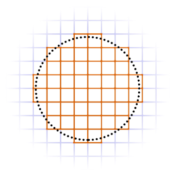
Figure 2: Two dimensional sketch of a staircase approximation (orange solid line) of a spherical particle (dotted).

The accuracy of this representation is only $O(1/R)$, $R$ being the radius of the sphere in lattice units, so that, in actual practice, the simulations always deal with rough spheres.

In accordance with the formulation proposed by F. Jansen and J. Harting [12], only the exterior regions are filled with fluid, whereas the interior parts of the particles are considered solid nodes. In the following, we designate as a boundary node, $\vec{r}_{b}$, all the fluid nodes linked by a vector $\vec{c}_{i}$ to a solid node, $\vec{r}_{s}=\vec{r}_{b}+\vec{c}_{i}$, of the particle. The solid–fluid interaction proceeds as follows. Since the particle surface (wall) of the staircase approximation is placed in the middle point of a lattice link, we identify pairs of mirror directions, denoted $(i,\bar{i})$, with $i$ oriented along the cut link hitting the particle surface and $\bar{i}$ directed in the opposite way, $\vec{c}_{\bar{i}}=-\vec{c}_{i}$. Hence, the populations hitting the particle surface are managed via a simple generalization of the halfway bounce-back rule [22] including the correction shown in Eq. 9 modelling the relative motion of the solid particle with respect to the surrounding fluid medium. Assuming a time step equal to one for simplicity, a post-collision population, $f^{\star}_{i}(\vec{r}_{b},t)$, hitting the wall along the cut link $i$ is reflected at the wall location, $\vec{r}_{w}=\vec{r}_{b}+\frac{1}{2}\vec{c}_{i}$, along the cut link $\bar{i}$ following the rule:

$$f_{\bar{i}}\left(\vec{r}_{b},t+1\right)=f_{i}^{\star}\left(\vec{r}_{b},t\right)-2w_{i}\rho\frac{\vec{u}_{w}\cdot\vec{c}_{i}}{c_{s}^{2}}.$$ (17)

The symbol $\vec{u}_{w}$ denotes the wall velocity of the $p$-th particle given by

$$\vec{u}_{w}=\vec{v}_{p}+\left(\vec{r}_{w}-\vec{r}_{p}\right)\times\vec{\omega}_{p}.$$ (18)

All coordinates with $p$-th as a subscript are relative to the center of the $p$-th particle, located at position $\vec{r}_{p}$ and moving with translation and angular velocities $\vec{v}_{p}$ and $\vec{\omega}_{p}$, respectively. Note that these rules reduce to the usual bounce-back conditions for a solid at rest, $\vec{v}_{p}=\vec{\omega}_{p}=0$. As a result of the reflection rule in Eq. 17, the force acting on the $p$-th particle at the wall location, $\vec{r}_{w}$, is

$$\begin{split}\vec{F}_{i}\left(\vec{r}_{w},t+\frac{1}{2}\right)=\left[f_{\bar{i}}\left(\vec{r}_{b},t+1\right)+f_{i}^{\star}\left(\vec{r}_{b},t\right)\right]\vec{c}_{i}=\\ =\left[2f_{i}^{\star}\left(\vec{r}_{b},t\right)-2w_{i}\rho\frac{\vec{u}_{w}\cdot\vec{c}_{i}}{c_{s}^{2}}\right]\vec{c}_{i}.\end{split}$$ (19)

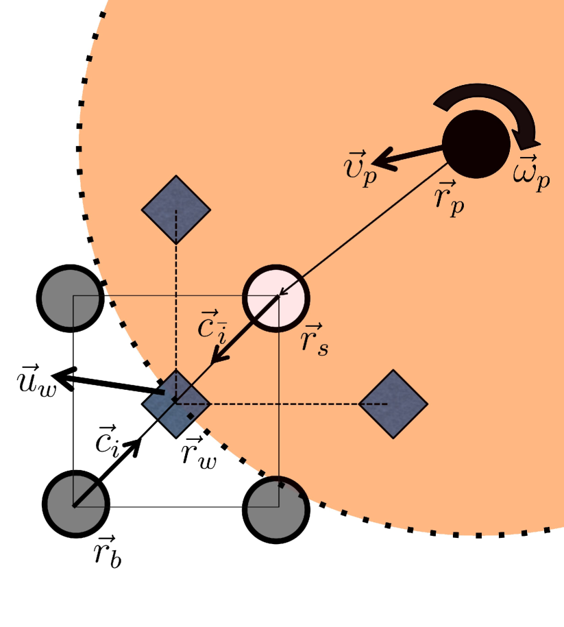
Figure 3: Head-on collisions along a link cutting through the staircased surface (diamonds). The actual surface is represented by the dotted line.

The different wettability of the particle surface provides a global unbalance of forces and a corresponding torque on the rigid body which is accounted by a variant approach of the model for hydrophobic fluid-surface interactions originally introduced by Benzi et al. [26] and extended to the realm of particle simulations in following works [12, 27]. In LBsoft, each solid node of the particle frontier is filled with a virtual fluid density. Hence, the virtual density at the node is taken as the average density value of the only fluid nodes $i_{\text{NP}}$ in the nearest lattice positions. In symbols, the virtual density of the $k$-th component reads

$$\bar{\rho}_{s}^{k}(\vec{r},t)=\left(1+\zeta_{ads}(\vec{r})\right)\frac{\sum_{i_{\text{NP}}}w_{i}\rho^{k}(\vec{r}+\vec{c}_{i},t)}{\sum_{i_{\text{NP}}}w_{i}},$$ (20)

where the average is weighted on the lattice stencil. Note that the average is multiplied by a prefactor including the constant $\zeta_{ads}(\vec{r})$, which tunes the local wettability of the solid node placed in $\vec{r}$. For $\zeta_{ads}>0$ the particle surface prefers the $k$-th fluid component, as for $\zeta_{ads}<0$ vice versa. Hence, the Shan-Chen force acting on the solid node is

$$\vec{F}^{k}_{s}(\vec{r},t)=\bar{\rho}^{k}_{s}(\vec{r},t)G_{C}\sum_{i}w_{i}\rho^{\bar{k}}(\vec{r}+\vec{c}_{i},t)s(\vec{r}+\vec{c}_{i},t)\vec{c_{i}},$$ (21)

where $s$ denotes a switching function that is equal to 1 or 0 for a fluid or solid node, respectively. The latter force term is counterbalanced by the Shan-Chen force exerted from the particle surface on the surrounding fluid, which is computed in Eq. 11 with the nodes filled with virtual fluid handled as regular fluid nodes.

The net force, $\vec{F}_{liq,\,p}$, acting from the surrounding fluid on the $p$-th particle is obtained by summing over all wall sites, $\vec{r}_{w}$, associated to the reflected links $i$, namely:

$$\vec{F}_{liq,\,p}=\sum_{{\vec{r}_{w},i}\in\Sigma_{p}}\vec{F}_{i}(\vec{r}_{w}).$$ (22)

Similarly, the corresponding torque, $\vec{T}_{liq,\,p}$, is computed as

$$\vec{T}_{liq,\,p}=\sum_{{\vec{r}_{w},i}\in\Sigma_{p}}\left(\vec{r}_{w}-\vec{r}_{p}\right)\times\vec{F}_{i}(\vec{r}_{w}).$$ (23)

Since particles move over the lattice nodes, it happens that a sub set of fluid boundary nodes, denoted $\{\vec{r}_{d}\}\in\mathcal{B}_{p}$, in front of a moving $p$-th particle cross its surface becoming solid nodes. Similarly, a sub set of interior nodes on the surface, $\{\vec{r}_{c}\}\in\Sigma_{p}$, are released at the back of the $p$-th moving particle. The two distinct events require the destruction and the creation of fluid nodes, respectively. In the destruction fluid node step, LBsoft pursues the straightforward procedure originally proposed by Aidun et al. [6]. Whenever a fluid node changes to solid, the fluid is deleted, and its linear and angular momenta are transferred to the particle. Given $\vec{r}_{d}$ the position vector of a deleted fluid node, the total force, $\vec{F}_{d,p}$, and torque, $\vec{T}_{d,p}$, on the $p$-th particle read

$$\vec{F}_{d,p} =\sum_{{\vec{r}_{d}}\in\mathcal{B}_{p}}\left[\rho^{k}(\vec{r}_{d})+\rho^{\bar{k}}(\vec{r}_{d})\right]\vec{u}(\vec{r}_{d}),$$ (24a)

$$\vec{T}_{d,p} =\sum_{{\vec{r}_{d}}\in\mathcal{B}_{p}}\left(\vec{r}_{d}-\vec{r}_{p}\right)\times\left\{\left[\rho^{k}(\vec{r}_{d})+\rho^{\bar{k}}(\vec{r}_{d})\right]\vec{u}(\vec{r}_{d})\right\},$$ (24b)

with the sum running over all the deleted fluid nodes, $\{\vec{r}_{s}\}\in\mathcal{B}_{p}$, of the $p$-th particle.

In the creation fluid node step, whenever the $p$-th particle leaves a lattice site located at $\vec{r}_{c}$ on its surface $\Sigma_{p}$, new fluid populations are initialized (see [6, 12]) from the equilibrium distributions, $f^{eq,k}_{i}(\bar{\rho}^{k},\vec{u}_{w})$, for the two $k$-th components with the velocity of the particle wall, $\vec{u}_{w}$ estimated via Eq. 18 and the fluid densities taken as the average values, $\bar{\rho}^{k}$ and $\bar{\rho}^{\bar{k}}$ respectively, of the neighbouring nodes. As a consequence of the creation fluid step, the associated linear and angular momenta, denoted $\vec{F}_{c,p}$ and $\vec{T}_{c,p}$, have to be subtracted from the $p$-th particle:

$$\vec{F}_{c,p} =\sum_{{\vec{r}_{c}}\in\Sigma_{p}}-\left[\rho^{k}(\vec{r}_{c})+\rho^{\bar{k}}(\vec{r}_{c})\right]\vec{u}_{w}(\vec{r}_{c}),$$ (25a)

$$\vec{T}_{c,p} =\sum_{{\vec{r}_{c}}\in\Sigma_{p}}\left(\vec{r}_{c}-\vec{r}_{p}\right)\times\left\{-\left[\rho^{k}(\vec{r}_{c})+\rho^{\bar{k}}(\vec{r}_{c})\right]\vec{u}_{w}(\vec{r}_{c})\right\},$$ (25b)

with the sum running over all the created fluid nodes, $\{\vec{r}_{c}\}\in\Sigma_{p}$, of the $p$-th particle.

Inter-particle interactions are handled by an extension of standard molecular dynamics algorithms. In particular, LBsoft implements the same strategy adopted by Jensen and Harting [12] to model hard spheres contact by an Hertzian repulsive force term. Thus, the repulsive contact force depends on the Hertzian potential according to the relation [28]

$$\vec{F}_{Hertz,\,i}=\begin{cases}-\frac{\partial}{\partial|\vec{r}_{i\,j}|}\left[K_{Hertz}\,\left(2\,R-|\vec{r}_{i\,j}|\right)^{\frac{5}{2}}\right]\frac{\vec{r}_{i\,j}}{|\vec{r}_{i\,j}|}&|\vec{r}_{i\,j}|<2\,R\\ 0&|\vec{r}_{i\,j}|\geq 2\,R\end{cases},$$ (26)

where $K_{Hertz}$ is an elastic constant and $\vec{r}_{i\,j}=(\vec{r}_{j}-\vec{r}_{i})$ the distance between $i$-th and $j$-th particles of radius $R$. Further, LBsoft implements a lubrication correction to recover the fluid flow description between two particle surfaces, whenever their distance is below the lattice resolution. Following the indications given by Nguyen and Ladd [29], the lubrication force reads

$$\vec{F}_{lub,\,i}=\begin{cases}-6\pi\nu\frac{R^{4}}{4R^{2}}\left(\frac{1}{h}-\frac{1}{h_{n}}\right)\left(\vec{\upsilon}_{i}-\vec{\upsilon}_{j}\right)\cdot\frac{\vec{r}_{i\,j}}{|\vec{r}_{i\,j}|}&h<h_{n}\\ \>\>0&h\geq h_{n}\end{cases},$$ (27)

where $h=(|\vec{r}_{i\,j}|-2\,R)$ and $h_{n}$ is a cut off distance. Note that the term $(\vec{\upsilon}_{i}-\vec{\upsilon}_{j})$ represents the relative velocity of the $i$-th particle with respect to the $j$-th one, so that a pair of perpendicularly colliding particles maximizes the repulsive lubrication force.

Finally, the total force and torque acting on the $p$-th particle reads

$$\vec{F}_{p} =\vec{F}_{liq,\,p}+\vec{F}_{d,p}+\vec{F}_{c,p}+\vec{F}_{Hertz,\,p}+\vec{F}_{lub,\,p},$$ (28a)

$$\vec{T}_{p} =\vec{T}_{liq,\,p}+\vec{T}_{d,p}+\vec{T}_{c,p}.$$ (28b)

We are now in a position to advance the particle position, speed $\vec{v}_{p}$ and angular momentum $\vec{\omega}_{p}$, according to Newton’s equations of motion:

$$\frac{d\vec{r}_{p}}{dt} =\vec{v}_{p},$$ (29a)

$$m_{p}\frac{d\vec{v}_{p}}{dt} =\vec{F}_{p},$$ (29b)

$$I_{p}\frac{d\vec{\omega}_{p}}{dt} =\vec{T}_{p},$$ (29c)

where $m_{p}$ and $I_{p}$ are the particle mass and moment of inertia, respectively.

The rotational motion of particles requires the description of the local reference frame of the particle with respect to the space fixed frame. For instance, denoted the local reference frame by the symbol $\star$, an arbitrary vector $\vec{d}^{\star}$ is transformed from the local frame to the space fixed frame by the relation

$$\vec{d}=\underline{\underline{\mathbf{R}}}\>\vec{d}^{\star},$$ (30)

where $\underline{\underline{\mathbf{R}}}$ denotes the rotational matrix to transform from the local reference frame to the space fixed frame. In order to guarantee a higher computational efficiency, LBsoft exploits the quaternion, a four dimensional unit vectors, $\mathbf{q}=[q_{0},q_{1},q_{2},q_{3}]^{T}$ in order to describe the orientation of the local reference frame of particles. In quaternion algebra[30], the rotational matrix , $\underline{\underline{\mathbf{R}}}$, can be expressed as

$$\underline{\underline{\mathbf{R}}}=\left(\begin{array}[]{ccc}q_{0}^{2}+q_{1}^{2}-q_{2}^{2}-q_{3}^{2}&2(q_{1}q_{2}-q_{0}q_{3})&2(q_{1}q_{3}+q_{0}q_{2})\\ 2(q_{1}q_{2}+q_{0}q_{3})&q_{0}^{2}-q_{1}^{2}+q_{2}^{2}-q_{3}^{2}&2(q_{2}q_{3}-q_{0}q_{1})\\ 2(q_{1}q_{3}-q_{0}q_{2})&2(q_{2}q_{3}+q_{0}q_{1})&q_{0}^{2}-q_{1}^{2}-q_{2}^{2}+q_{3}^{2}\\ \end{array}\right),$$ (31)

whereas the transformation of a vector $\vec{d}^{\star}$ from the local frame to the space fixed frame is obtained as $\vec{d}=\mathbf{q}\>\vec{d}^{\star}\mathbf{q}^{-1}$, and vice versa as $\vec{d}^{\star}=\mathbf{q}^{-1}\vec{d}\>\mathbf{q}$.

Exploiting the quaternion representation, the particles are advanced in time according to the rotational leap-frog algorithm proposed by Svanberg [31]:

$$\vec{v}_{p}\left(t+\frac{1}{2}\right)=\vec{v}_{p}\left(t-\frac{1}{2}\right)+\frac{\vec{F}_{p}\left(t\right)}{m_{p}},$$ (32a)

$$\vec{r}_{p}\left(t+1\right)=\vec{r}_{p}\left(t\right)+\vec{v}_{p}\left(t+\frac{1}{2}\right),$$ (32b)

$$\vec{\omega}_{p}^{\star}\left(t+\frac{1}{2}\right)=\vec{\omega}_{p}^{\star}\left(t-\frac{1}{2}\right)+\frac{\vec{T}_{p}^{\star}\left(t\right)}{I_{p}^{\star}},$$ (32c)

$$\mathbf{q}_{p}\left(t+1\right)=\mathbf{q}_{p}\left(t\right)+\dot{\mathbf{q}}_{p}\left(t+\frac{1}{2}\right),$$ (32d)

where $\dot{\mathbf{q}}=[\dot{q}_{0},\dot{q}_{1},\dot{q}_{2},\dot{q}_{3}]^{T}$ denotes the quaternion time derivative of the $p$-th particle. Since the quaternion time derivative reads

$$\left(\begin{array}[]{cccc}\dot{q}_{0}\\ \dot{q}_{1}\\ \dot{q}_{2}\\ \dot{q}_{3}\\ \end{array}\right)=\frac{1}{2}\left(\begin{array}[]{cccc}q_{0}&-q_{1}&-q_{2}&-q_{3}\\ q_{1}&q_{0}&-q_{3}&q_{2}\\ q_{2}&q_{3}&q_{0}&-q_{1}\\ q_{3}&-q_{2}&q_{1}&q_{0}\\ \end{array}\right)\left(\begin{array}[]{cccc}0\\ \omega^{\star}_{x}\\ \omega^{\star}_{y}\\ \omega^{\star}_{z}\\ \end{array}\right),$$ (33)

the reckoning of $\dot{\mathbf{q}}_{p}\left(t+\frac{1}{2}\right)$ requires the evaluation of $\mathbf{q}_{p}\left(t+\frac{1}{2}\right)$ which is not known at time $t+\frac{1}{2}$. Svanberg [31] overcomes the issue exploiting Eq. 32d integrated at half time step, so obtaining the implicit equation

$$\mathbf{q}_{p}\left(t+\frac{1}{2}\right)=\mathbf{q}_{p}\left(t\right)+\frac{1}{2}\dot{\mathbf{q}}_{p}\left(t+\frac{1}{2}\right),$$ (34)

which is solved by iteration, taking as a starting value $\mathbf{q}_{p}(t+\frac{1}{2})=\mathbf{q}_{p}(t)+\frac{1}{2}\dot{\mathbf{q}}_{p}(t)$ to estimate via Eq. 33 the time derivative $\dot{\mathbf{q}}_{p}(t+\frac{1}{2})$ . As the updated value of $\mathbf{q}_{p}(t+\frac{1}{2})$ is assessed by Eq. 34, the procedure is repeated until the term $\dot{\mathbf{q}}_{p}(t+\frac{1}{2})$ converges.

Note that the force, $\vec{F}_{liq,\,p}$, and torque, $\vec{T}_{liq,\,p}$ , exerted from the fluid on the particles are computed at half-integer times. Therefore, the total force and torque are assessed as

$$\begin{split}\vec{F}_{p}(t)&=\frac{\vec{F}_{liq,\,p}(t-\frac{1}{2})+\vec{F}_{liq,\,p}(t+\frac{1}{2})}{2}+\vec{F}_{d,p}(t)+\vec{F}_{c,p}(t)+\\ &+\vec{F}_{Hertz,\,p}(t)+\vec{F}_{lub,\,p}(t),\end{split}$$ (35a)

$$\vec{T}_{p}(t) =\frac{\vec{T}_{liq,\,p}(t-\frac{1}{2})+\vec{T}_{liq,\,p}(t+\frac{1}{2})}{2}+\vec{T}_{d,p}(t)+\vec{T}_{c,p}(t).$$ (35b)

The set of Equations 32 takes into account the full many-body hydrodynamic interactions, since the forces and torques are computed with the actual flow configuration, as dictated by the presence of all $N$ particles simultaneously.

3 Implementation

LBsoft is implemented in Fortran 95 using modules to minimize code cluttering. In particular, the variables having in common the description of certain features (e.g., fluids and particles) or methods (e.g., time integrators) are rounded in different modules. The code adopts the convention of the explicit type declaration with PRIVATE and PUBLIC accessibility attributes in order to decrease error-proneness in programming. Further, the arguments passed in calling sequences of subroutines have defined intent.

LBsoft is written to remain portable with ease (multi-architecture) and readable (to allow code contribution), as much as possible taking into account the complexity of the underlying model

LBsoft has been developed, from the very beginning, considering, as target, parallel computing platforms. The communication among computing nodes exploits the de-facto standard Message Passing Interface (MPI). The communication in LBsoft is implemented in the module version_mod contained in the parallel_version_mod.f90 file. Note that the module module version_mod is also provided in a serial version located in the serial_version_mod.f90 file, which can be easily selected in the compiling phase (see below).

LBsoft is completely open source, available at the public repository on GitHub: www.github.com/copmat/LBsoft under the 3-Clause BSD License (BSD-3-Clause).

The repository is structured in three directories: source, tests, and execute.

All the source code files are contained in the source directory. The code does not require external libraries, and it may be compiled on any UNIX-like platform. To that purpose, the source directory contains a UNIX makefile to compile and link the code into the executable binary file with different compilers. The makefile includes a list of targets for several common compilers and architectures (e.g., Intel Skylake, and Intel Xeon Phi) are already defined in the makefile with proper flags for the activation of specific instruction sets, such as the 512-bit Advanced Vector Extensions (AVX-512). The list can be used by the command “make target”, where target is one of the options reported in Tab 1. On Windows systems we advice the user to compile LBsoft under the command-line interface Cygwin [32] or the Windows subsystem for Linux (WSL).

The tests directory contains a set of test cases for code validation and results replication. The test cases can also help the user to create new input files. Further, the folder contains also a simple tool for running all of them and checking results: this simplifies working with the code as it quickly detects when a set of changes break working features. Along with code versioning (using git and public repository GitHub), this can also lead to automatic search of problematic code changes through the bisection git capability.

Finally, the binary executable file can be run in the execute directory.

target:	meaning:
gfortran	GNU Fortran compiler in serial mode.
gfortran-mpi	GNU Fortran compiler in parallel mode with Open Mpi library.
intel	Intel compiler in serial mode.
intel-mpi	Intel compiler in parallel mode with Intel Mpi library.
intel-openmpi	Intel compiler in parallel mode with Open Mpi library.
intel-mpi-skylake	Intel compiler in parallel mode with Intel Mpi library
	and flags for Skylake processor features (AVX-512 activated).
intel-mpi-knl	Intel compiler in parallel mode with Intel Mpi library
	and flags for Xeon Phi processor features (AVX-512 activated).
help	return the list of possible target choices

Table 1: List of targets for several common parallel environments, which can be used by the command "make target".

The source code is structured as follows: the main.f90 file implements the execution flow of LBsoft, gathering in sequence the main stages, which are initialization, simulation, and finalization. The initialisation stage includes the reading of the input file input.dat, describing the simulation setup and the physical parameters of the simulation. Further details on the input parameters and directives are reported below in Section 4. Moreover, the initialization stage involves the allocation of main data arrays, as well as their initialization. At this stage, the global communication among computing nodes is set up, and the simulation mesh is decomposed in sub-domains, each one assigned to a node.

The simulation stage solves both the lattice-Boltzmann equation and, if requested, the particles evolution for the simulation time specified in the input file. The fluids_mod.f90 and particles_mod.f90 files collect all variable declarations, relative definitions, and procedures dealing with fluids and particles, respectively. In the simulation stage, several statistical observables of the system are computed at prescribed time steps by suitable routines of the statistic_mod.f90 file. The observables can be printed on the output file, statdat.dat, in several forms defined by specific directives in the input file. Further, the savings of fluid density and flow fields alongside with particle positions and orientations can be activated in the input file and stored in different output formats.

Finally, the finalisation stage closes the global communication environment, deallocates previously allocated memory, and write a the restart files before the program closes successfully.

In the following Subsection, a few key points of the model implementation will be outlined in more detail.

3.1 Algorithmic details

The time-marching implementation of the lattice-Boltzmann equation (Eq. 1) can be realized by different approaches: the two-lattice, two-step, and fused swap algorithms, to name a few [33, 34, 35, 36]. All these implementations manage the collision (Eq. 2) and streaming (Eq. 3) steps following a different treatment of data dependence. For instance, since the streaming step is not a local operation, it can be implemented with a temporary copy in memory of old values for not overwriting locations in the direction of $\vec{c}_{i}$, or with a careful memory traversal in direction opposite to $\vec{c}_{i}$, thus avoiding memory copies.

The two steps can be fused in one, for maximal reuse of data after fetching from memory and to avoid latencies in the streaming step (fused algorithm), at the cost of code complexity and increased level of difficulty in experimenting with different force types. The interaction of the particle solver makes this fused approach even more challenging, since force on particles are needed at intermediate time steps with respect to LB times.

LBsoft implements the more modular form provided in the two-step algorithm [34]. Indeed, the shift algorithm preserves separate subroutines or functions to compute the hydrodynamic variables, the equilibrium distributions, the collision step and the streaming step. The highly modular approach of the shift algorithm allows a simpler coupling strategy to the particle solver.

The main variables of the code are the 19 distributions, the recovered physical variables ($\rho$,$\vec{u}$) and a 3D field of booleans indicating whether the lattice point is fluid or not (a particle or an obstacle). The LB distributions are usually stored in two different memory layouts which are mutually conflicting. Regardless of the memory order (row-major like in C or column-major as in FORTRAN), the npop populations of the 3-d lattice of size [nx,ny,nz] can be stored as an array of structures (AoS) or as a structure of arrays (SoA) [36].

The chosen memory layout in LBsoft is the SoA, which proved to be more performing than the AoS layout. In particular, the streaming step in the SoA reduces to a unitary stride. Hence, the SoA layout is optimal for streaming with a significant decrease in memory bandwidth issues.

In order to solve the lattice-Boltzmann equation, the algorithm proceeds by the following sequence of subroutine calls:

1. Recover density and velocity from populations (using Eq. 6 and Eq. 7);

2. Compute the force term if necessary (e.g., Eq. 11);

3. Compute populations after collision (using Eqs 2 and 5);

4. Apply halfway bounce-back rules (e.g., Eq. 8);

5. Stream populations (using Eq. 3).

Note that for the coupling forces between fluids, two subroutines deal with the evaluation of the pseudo potential fields and their gradients, respectively, in order to assess Eq. 11. Hence, the coupling force is added into the LB scheme as in Eq. 16 to perform the collision step. In the tests, a dedicated test is present in the 3D_Spinoidal folder to simulate the separation of two fluids in two complete regions.

In the case of particle simulation, the sequence of subroutine calls is:

1. Recover density and velocity from populations (using Eq. 6 and Eq. 7);

2. Destroy and create fluid nodes according to moving particles and compute relative force correction terms (using Eqs 24 and 25);

3. Compute the forces among particles (using Eqs 26 and 27);

4. Compute the LB force term (using Eq. 20 and 21);

5. Compute populations for eack component after LB collision (using Eqs 2 and 5);

6. Apply the halfway bounce-back rule at particle surface and the relative force terms on particles (using Eqs 17 and 19);

7. Evolve position and angular velocity of particles (using Eq. 32);

8. Stream populations for each component (using Eq. 3).

It is worth to stress that the net force and torque exerted from the fluid on a particle (step 6 in the previous scheme) is obtained by summing over all wall sites of the surface particle as reported in Eqs 22 and 23. These summations add several numerical terms of opposite signs, giving results having a very small value in magnitude (close to zero if the surrounding fluid is at rest). The finite numerical representation in floating-point arithmetic leads to loss of significance in the sum operator due to the round-off error. The issue is observed in LBsoft, as the summation order is modified, providing different results of the arithmetic operation up to the eighth decimal place in double-precision floating-point format. Whenever the accuracy of the particle trajectories is essential, it is possible to compile LBsoft with the preprocessor directive QUAD_FORCEINT in order to perform these summations in quadruple-precision floating-point format, recovering the loss of significance.

The motion of the colloidal particles (step 7 in the previous scheme) is numerically solved by a leapfrog approach. In particular, the evolution of the angular moment is treated by the leapfrog-like scheme proposed by Svanberg [31], also referred to as mid-step implicit algorithm (see Eqs 32 and 34). The mid-step scheme was adopted after the implementation of different time advancing algorithms and after the evaluation of their numerical precision by a test case. In particular, the test examined a rotating particle in a still fluid, measuring the numerical accuracy at which the code simulates a complete revolution with no energy drift. The tested schemes were full-step [37], the mid-step [31] and the simple leapfrog versions. The mid-step implicit leapfrog-like algorithm was found to be more consistent with respect to other rotational leapfrog schemes, confirming previous observations in literature [38, 31].

The inter-particle force computation exploits the neighbour lists, which track the particles close to each $p$-th particle within a distance cut-off rcut. The list is constructed by a combination of the link-cell algorithm with the Verlet list scheme [39, 40, 41]. Briefly, this strategy avoids the evaluation of the neighbour list at each time step, limiting the list update only to the cases in which a particle moves beyond a tolerance displacement, delr, given as an input parameter. As the lists need to be updated, the link-cell algorithm allows for the location of interacting particles with a linearly scaling cost, $O(N)$, being $N$ the total number of particles.

The comprehensive algorithmic organization for colloidal simulations provides a clear structure for the possible integration of future features. Indeed, the extensibility of the steps was overall preferred, preserving, as much as possible, the computational performances.

3.2 Parallelization

LBsoft is parallelized according to the single program multiple data paradigm [42] using the Message Passing Interface (MPI) protocol. In particular, the parallelization of the hydrodynamic part exploits the domain decomposition (DD) [43] of the simulation box using a one-, two- or three-dimensional block distribution among the MPI tasks. The selection of the block distribution is done at run-time (without recompiling the source code), and it can be tuned to obtain the best performance given the global grid dimension and the number of computing cores. In the case of a cubic box, the best performance corresponds to the three-dimensional DD, which minimizes the surface to be communicated. The current version of LBsoft features a halo having a width of one lattice spacing, which is necessary to compute the local coupling force between the two fluid components. Actually, the halo width could be easily increased for future algorithms.

Two main parallelization strategies, replicated data (RD) [44, 45] and domain decomposition [46, 47], have been considered for the particle evolution in order to balance and equally divide the computation of particle dynamics among available cores, minimizing the amount of transmitted data among nodes. The worst case scenario is a lattice cube with 20% of the volume occupied by particles of radius in a range from 5.5 to 10 lattice nodes. Even in this extreme condition, the number of particles is in the order of 10K-20K, to be compared with lattice size of $1024^{3}$ (1G nodes). Given the relative limited number of particles, the Replicated Data (RD) parallelization strategy has been adopted in LBsoft.

The RD strategy generally increases the amount of transmitted data in global communications, nonetheless the method is relatively simple to code and reasonably efficient for our cases of interest. Within this paradigm, a complete replication of the particle physical variables (position, velocity, angular velocity) among the MPI tasks is performed. In particular, $\vec{r}_{p}$, $\vec{v}_{p}$ and $\vec{\omega}_{p}$ are allocated and maintained in all MPI tasks, but each MPI task evolves Eq. 32 only for particles whose centers of mass lie in its sub-domain defined by the fluid partition. Since each task evolves in time the particles residing in its local fluid sub-domain, the fluid quantities around each $p$-th particle (apart for the standard 1-cell halo needed for the streaming part of the LB scheme) does not require to be transferred to the task in charge of the particle. In this way, the interactions between particles and surrounding fluid are completely localized without the need of exchanging data among tasks. Only in the case of a particle crossing two or more sub-domains, the net quantities of force and torque acting from the fluid on the particle (Eqs 22 and 23) are assessed at the cost of some global MPI reduction operations while performing the time advancing. After the time step integration, new values of $\vec{r}_{p}$, $\vec{v}_{p}$ and $\vec{\omega}_{p}$ are sent to all tasks. It is worth to highlight that the distribution of particles among MPI tasks (LB managed) may show unbalance issues, particularly in particle aggregation processes where the particle density locally increases in correspondence of clustered structures. Nonetheless, the cases studied so far do not show pathological effects due to workload unbalance.

4 Description of input and output files

LBsoft needs an input file to setup the simulation. The input file is free-form and case-insensitive. The input file is named input.dat, and it is structured in rooms. Each room starts with the directive [room "name"] bracket by square brackets, and it finishes with the directive [end room]. The [room system], [room fluid], and [room particle] compose the list of possible choices. The main room is the [room system], which specifies the number of time steps to be integrated, the size of the simulation box, the boundary conditions, the type of adopted domain decomposition declares (1D, 2D, or 3D), and the directives invoking the output files. The other two rooms, [room fluid] and [room particle], provide specification of various parameters for the two actors, respectively. A list of key directives for each room is reported in A for the benefit of potential LBsoft users. Just few of these directives are mandatory. A missed definition of any mandatory directive will call an error banner on the standard output. In each room, the key directives can be written without a specific order. Every line is read as a command sentence (record). Whenever a record begins with the symbol # (commented), the line is not processed. Each record is parsed in words (directives and additional keywords and numbers) with space characters recognized as separator elements. Finally, the [end] directive marks the end of the input data. In the current software version all the quantities have to be expressed in lattice units.

In the case of particles simulation, a second input file, named input.xyz, has to be specified. The input.xyz file contains the specification of position, orientation, and velocity of particles. The file is structured as follows: the first record is an integer indicating the particle number, while the second may be empty or report the directive read list followed by appropriate symbolic strings, whose meaning is reported in B. Hence, a sequence of $N$ lines follows with $N$ the number of particles. Each line reports a character string identifying the particle type, the position coordinates, $x$ $y$ $z$, and, if the directive read list was specified at the second record, a sequence of floating point numbers specifying the values of the parameters following the directive read list.

Specific directives cause the writing of output files in different formats (see A). Mainly, LBsoft prints on the standard output. The reported information regards the code initialization, time-dependent data of the running simulation, warning and error banners in case of problems during the program execution. The data reported in the standard output can be selected using the directive print list followed by appropriate symbolic strings. We report in C the list of possible symbolic strings. Hence, the selected data are printed at the time interval indicated by the directive print every. The next Section delivers few examples of input.dat files.

The directive print vtk triggers the writing of the fluid density and flow fields in a format compatible with the visualization toolkit (VTK) [48]. Whenever particles are present, their position and orientation are also written in a VTK compatible format. The VTK format files can be read by common visualization programs (e.g., ParaView [49]). Further, the directive print xyz provides the writing of a file traj.xyz with the particle positions written in XYZ format and readable by suitable visualization programs (e.g. VMD-Visual Molecular Dynamics [50]) to generate animations.

Finally, a simple binary output of relevant data can be activated by the key directive print binary. Each Eulerian field will be saved as a unique file in a simple binary matrix (or vector for scalar fields) resorting to the parallel input/output subroutines available in the MPI library. The last strategy is the fastest and more compact writing mode currently implemented in LBsoft.

5 Test cases and performance

LBsoft provides a set of test cases in a dedicated directory. Several physical scenarios verify the code functionalities testing all the implemented algorithms. Among them, there are the Shear flow and the Pouseille flow in all the possible Cartesian directions in order to test boundary conditions, forcing scheme, and, in general, the LB implementation (2D_Shear and 2D_Poiseuille sub-folders). The spinoidal decomposition of two fluids in 3D inquires the functionality of Shan-Chen force algorithm. Several tests containing a single particle serve to check the translation (3D_Particle_pbc folder) and rotational part of the leapfrog integrator (3D_Shear_Particle and 3D_Rotating_Particle sub-folders).

These examples can be used to understand the capabilities of the code, to become familiar with input parameters (looking at the input.dat files), and to check that code changes do not compromise basic behaviour (the so called “regression testing”).

Complex simulations require a code able to deliver good performance with robust scaling properties. In order to assess the performance of LBsoft, three cases were selected. The corresponding input files are briefly described below.

We probe the efficiency of the implemented parallel strategy of LBsoft by quantitative estimators. In order to measure the performance of the LB solver, the Giga Lattice Updates Per Second (GLUPS) unit is used. In particular, the definition of GLUPS reads:

$$\text{GLUPS}=\frac{L_{x}L_{y}L_{z}}{10^{9}t_{\text{s}}},$$ (36)

where $L_{x}$, $L_{y}$, and $L_{z}$ are the domain sizes in the $x-$, $y-$, and $z-$ axis, and $t_{\text{s}}$ is the run (wall-clock) time (in seconds) per single time step iteration. We also report the estimator MLUPSCore defined as the Lattice Updates Per Second and Per computing core:

$$\text{MLUPSCore}=\frac{L_{x}L_{y}L_{z}}{10^{6}t_{\text{s}}\,n_{p}},$$ (37)

where $n_{p}$ denotes the number of processor cores.

Further, the speedup ($S_{p}$) is defined as

$$S_{p}=\frac{T_{s}}{T_{p}},$$ (38)

where $T_{s}$ stands for the CPU wall-clock time of the code executed on a single core, taken as a reference point, and $T_{p}$ is the CPU wall-clock time of the code in parallel mode executed by a number of processors equal to $n_{p}$ .

Hence, the parallel efficiency ($E_{p}$) is defined as

$$E_{p}=\frac{S_{p}}{n_{p}}.$$ (39)

The benchmarks were carried out on two different computing platforms:

• a cluster of servers each with 2 Intel Xeon Gold 6148 clocked at 2.8 GHz (20-core cpu), for a total of 40 cores per node, with 192 GB of DDR4, in the following labelled $(a)$;

• a cluster of servers each with 1 Intel Xeon Phi 7250 clocked at 1.4 GHz (68-core cpu), for a total of 68 cores per node, with 16 GB of MCDRAM and 96 GB of DDR4, in the following labelled $(b)$.

In all the following benchmarks, the LBsoft source code was compiled using the Intel Fortran Compiler, version 2018, with the proper flags to activate the Advanced Vector Extensions 512-bit (AVX-512) instructions. The MPI library implementation provided by Intel was exploited to manage the parallel communications. Hence, results and comments are below reported.

5.1 Benchmarks

In order to evaluate the computational performance of the lattice Boltzmann solver alone, we consider two cubic boxes of side 512 and 1024 lattice nodes with periodic boundary along the three Cartesian axes. The boxes are randomly filled with fluid mass density equal to 1.0 and zero velocity flow field (see benchmark test 1 in D).

Table 2 reports the wall-clock time measured on the computing platform $(a)$ as a function of the cores number (strong scaling) for both the box sizes alongside with the corresponding speed up, $S_{p}$, and parallel efficiency, $E_{p}$. We also reports the LB performance metrics in terms of GLUPS, as defined in Eq. 36.

$n_{p}$	$t_{\text{s}}$ (s)	GLUPS	MLUPSCore	$S_{p}$	$E_{p}$
128	0.294	0.46	3.59	1.00	100%
256	0.152	0.88	3.44	1.92	96%
512	0.079	1.70	3.32	3.68	92%
1024	0.046	2.92	2.85	6,32	79%
2048	0.025	5.37	2.62	11.52	72%
128	2.173	0.49	3.83	1.00	100%
256	1.159	0.93	3.63	1.86	93%
512	0.595	1.80	3.52	3.64	91%
1024	0.321	3.34	3.26	6.72	84%
2048	0.165	6.51	3.18	13.12	82%

Table 2: Run (wall-clock) time in seconds per single time step iteration, $t_{\text{s}}$, with corresponding GLUPS, MLUPSCore, speed up, $S_{p}$, and parallel efficiency, $E_{p}$, versus the number of computing cores, $n_{p}$ for a single component fluid simulation. From the top to bottom, results are reported for a cubic box of side $512$ and $1024$. Note that the parallel efficiency is reported in percentage.

Here, the parallel efficiency is higher than 90% up to 512 cores (see Tab. 2). Nonetheless, it is apparent that the efficiency decreases with the increase of the communication burden (due to the high number of cores). This is commonly due to the communication latency, which deteriorates the performance whenever the workload assigned to each processor is not sufficiently high to offset the communication overheads. Hence, larger box sizes guarantees a high parallel efficiency also with a high number of computing cores, as shown in Tab. 2 for the larger box size case under investigation ($E_{p}\simeq 80\%$ even on 2048 coresze).

The comparison between the two cases provides insights also on the weak scaling properties of LBsoft. In particular, it is observed an increase in the wall-clock time of a factor close to eight scaling from the smaller (512) up to the larger (1024) box size, confirming a quasi linear weak scaling behaviour. It is worth to highlight that the code performance are generally comparable with that observed in literature [36, 51] following a similar implementation strategy of keeping separated the collision and streaming steps.

The entire LBsoft machinery is tested on the two component LB fluid model (see Subsection 2.3) combined with the particle solver (Subsection 2.4) describing the colloids in a rapid demixing emulsion. In order to assess the performance of the particle solver, we defined three simulation setups with different numbers of particles. In particular, three cubic boxes having a side of 245, 512 and 1024 lattice nodes were respectively filled with two fluids randomly distributed with initial fluid densities extracted from a Gaussian distribution of mean and standard deviation equal to 1.0 lu and 0.004 lu, respectively. Hence, three values of the volume fraction occupied by particles are considered: 1%, 10% and 20%, labeled $case\;1$, $case\;2$, and $case\;3$, respectively.

The benchmark results will be also compared to the corresponding box sizes without particles, labeled $case\;0$ (input file 2 reported in D). In all the cases, the Shan-Chen force term (see Subsection 2.3) is activated by the key directive force shanchen pair, which serves also to set the coupling constant value equal to 0.65 lu. The particles are assumed having all the same radius equal to 5.5 lu, and are randomly distributed in the box. The initial particle velocity was set equalt to zero by the key directive initial temperature 0.d0 (see input-file-3 of D). The particle wettability is set with an angle equal to $108^{\circ}$ with respect to the main axis $\vec{x}^{\star}$ in the local reference frame of each particle (key directive force shanchen angle). Note that the wettability is tuned by a smoothed switching function of the wettability angle, varying from -1 to 1 in a given range (in this case $10^{\circ}$) around the target value of $108^{\circ}$. All the inter-particle force terms were computed by means of neighbor’s lists built with the shell distance cutoff equal to 12 lu, augmented by a tolerance value equal to 1 lu, set by the key directives rcut and delr, respectively. The lubrication force is activated from a 2/3 lattice mutual distance between two particles, as reported in previous simulations [12]. Further, the Hertzian repulsive potential starts as soon as two particles are closer than one lattice unit in order to avoid particle overlay events. The particle mass was estimated as the weight corresponding to a particle made of silica [52].

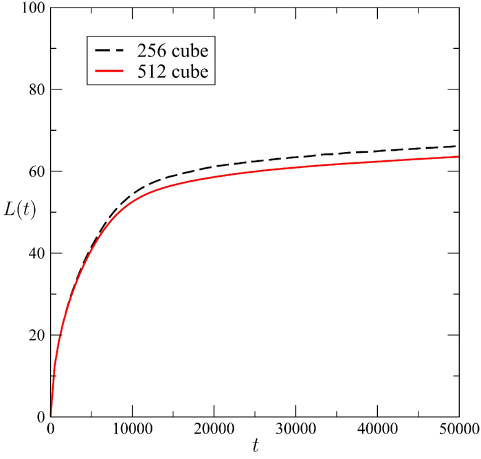
Figure 4: Average domain size over time for the two systems of cubic side 256 and 512 at 20% in particle volume fraction. After a rapid growth of the domain size to over 60 lattice units during the first 20000 time steps, the $L(t)$ trend is stable close to the asymptotic value of 70 lattice units.

Figure 5: 3D visualization of the system with cubic box of side 512 lattice units described in Figure 4 at four different times. The particles are located close to the interface between the fluid components. While the change in the particle configuration is evident from time steps 2000 up to 10000 (labelled $a$ and $b$, respectively), the domain growth is almost at rest in the following snapshots (snapshot $c$ and $d$) The density colour map is referred to the red fluid component.

The test case describes the phase separation dynamics of two immiscible liquids which is arrested in a rigid state by a jammed layer of colloidal particles located at the interface. The final metastable state is a bi-continuous interfacially jammed emulsion gel, also referred to as a bi-jel [53]. The resulting dynamics can be described in terms of the average domain size measured along the time evolution, denoted $L(t)$ in the following text. Here, $L(t)$ is expected to show an asymptotic behaviour as the jammed layer arrests the domain growth, whereas in absence of colloidal particles $L(t)$ increases, showing a stretched exponential trend in the average domain size [54]. Several definitions of the average domain size were proposed in literature [55, 54, 56, 57]. Here, the average size of domains is defined as the inverse of the first moment of the structure factor, $S(k,t)$, averaged on a sphere of radius $k$, being $k=|\vec{k}|$ the modulus of the wave vector in Fourier space. Thus, $L(t)$ reads:

$$L(t)=2\pi\frac{\displaystyle\int S(k,t)\mathrm{d}k}{\displaystyle\int kS(k,t)\mathrm{d}k}\>\text{,}$$ (40)

being $S(k,t)\equiv\langle\phi^{{}^{\prime}}(\vec{k},t)\phi^{{}^{\prime}}(-\vec{k},t)\rangle$ with $\phi^{{}^{\prime}}(\vec{k},t)$ the spatial Fourier transform of the fluctuations of the order parameter $\phi^{{}^{\prime}}=(\phi-\langle\phi\rangle)$. The order parameter $\phi$ is the phase field of the two components, called red and blue, $\phi=(\rho_{r}-\rho_{b})/(\rho_{r}+\rho_{b})$.

Figure 4 shows the average domain size versus time, $L(t)$, for the simulation box sizes of $256^{3}$ and $512^{3}$ lattice nodes with 5000 and 40000 particles, respectively, corresponding to case (3) with 20% in particle volume fraction. Here, the $L(t)$ trend clearly shows an initial increase due to a brief period of phase decomposition up to about 20000 time steps. After this initial jump, the asymptotic behaviour is observed for both the box sizes with the converging value close to $\sim 70$ lattice units. The result is in agreement with similar observations in literature [12, 58], validating the colloidal particle implementation in LBsoft. The arrest of the phase demixing process is also evident by visualizing the set of snapshots taken at different times (reported in Fig. 5) for the cubic box of side 512. In particular, Figure 5 clearly shows as the particles located at the fluid-fluid interface entrap the demixing process into a metastable state, the bi-continuous jammed gel state.

$n_{p}$	$t_{\text{s}}$ (s)	GLUPS	MLUPSCore	$S_{p}$	$E_{p}$
128	6.012	0.18	1.41	1.00	100%
256	2.9	0.37	1.45	2.06	103%
512	1.484	0.72	1.41	4.04	101%
1024	0.784	1.37	1.34	7.60	95%
128	6.4	0.17	1.33	1.00	100%
256	3.63	0.30	1.17	1.76	88%
512	2.12	0.51	1.00	3.04	76%
1024	1.40	0.76	0.45	4.56	57%
128	8.42	0.13	1.02	1.00	100%
256	4.79	0.22	0.86	1.76	88%
512	2.77	0.39	0.76	3.04	76%
1024	1.96	0.55	0.54	4.32	54%
128	10.53	0.10	0.78	1.00	100%
256	6.00	0.18	0.70	1.76	88%
512	3.63	0.30	0.59	2.92	73%
1024	2.61	0.41	0.40	4.00	50%

Table 3: Run (wall-clock) time, in seconds, per single time step iteration, $t_{\text{s}}$, with corresponding GLUPS, MLUPSCore, speed up, $S_{p}$, and parallel efficiency, $E_{p}$, versus the number of computing cores, $n_{p}$ for a two component fluid in a cubic box of side $1024$ without particles (case 0), and with three numbers of colloidal particles, $N$ (cases 1,2 and 3). From the top to the bottom, the box $1024^{3}$ was filled with $N=0$, $N=15407$, $N=154072$, and $N=308144$ (corresponding to a particle volume fraction equal to 0%, 1%, 10% and 20%, respectively). Note that the parallel efficiency is reported in percentage.

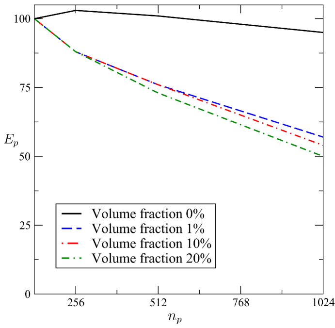
Figure 6: Parallel efficiency, $E_{p}$, measured in a cubic box of $1024$ with different values in particle volume fraction versus the number of computing cores, $n_{p}$. Note that the $E_{p}$ is reported in percentage.

Table 3 reports the strong scaling of wall-clock time per iteration step, $t_{\text{s}}$, as a function of the core number, $n_{p}$, for the cubic box of side 1024 filled with different numbers of particles. The respective GLUPS and parallel efficiency, $E_{p}$, are also reported in Tab. 3. The measurements are carried out for all the three values of volume fraction under investigation (case 1, 2, and 3). In particular, the comparison among the three cases provides valuable information on the performance scaling as a function of the particle number in order to probe the weight of the MD part on the simulation time.

As a first observation, the measured wall-clock timings are about 2 and 3 times higher than the corresponding values measured in the single-fluid case under the same conditions of cores number and box size. The last finding is in agreement with previous observations reported in the literature [36, 51].

In Tab. 3, the simulations of $case\;0$ without particles show wall-clock times which are about 2 and 3 higher than the corresponding values measured in the single-fluid case under the same conditions of cores number and box size. The last finding is in agreement with previous observations reported in the literature [36, 51].

Whenever the particle solver is activated, the parallel efficiency, $E_{p}$, remains above 50% in all the three cases under investigation (see Fig. 6). As a matter of fact, although it is apparent that the particle solver degrades the performance of the entire simulation, that decrease in $E_{p}$ is comparable to codes specifically designed for molecular dynamics simulations (e.g. LAMMPS [59], DL_poly [60], etc.). For instance, a simulation of Lennard-Jones liquid of 30000 atoms shows in LAMMPS code a parallel efficiency, $E_{p}$, oscillating from 10% up to 40% on 512 cores depending on the computing architecture [61].

Nonetheless, the analysis of the performance as a function of the number of particles shows a clear bottle-neck, going from 1% to 20% in the particle volume fraction. Here, the parallel efficiency is not scaling with the harder workload per core in the particle number, $N$. This is likely due to the Replicated Data strategy adopted in the implementation of the particle solver in LBsoft. In order to recover the parallel efficiency in the particle scaled-size problem, further code tuning is ongoing. The most promising strategy involves a mixed OpenMP + MPI parallelization, in which the code utilises only a few MPI processes per node, and exploits all cores of a node with no explicit communication using OpenMP. This paradigm will reduce consistently the MPI global communications needed for the evolution of the particles with overall benefits in the parallel efficiency.

Finally, the code was also tested in the same conditions on a cluster of servers based on Intel KNL processors, computing architecture (b), courtesy of CINECA supercomputing center. Regardless of changes introduced to let the Intel Fortran compiler provide a better optimisation of the code, we observed a factor close to three of performance degradation in all the conditions under investigations. Apart the obvious lower clock frequency, the quite poor result may be motivated by a sub-optimal exploitation of the limited MCDRAM size (16 GB) in the Intel Xeon Phi processor, which could be improved using arbitrary combinations of MPI and OpenMP threads within an hybrid parallel implementation paradigm [62].

5.2 New applications: confined bijels under shear

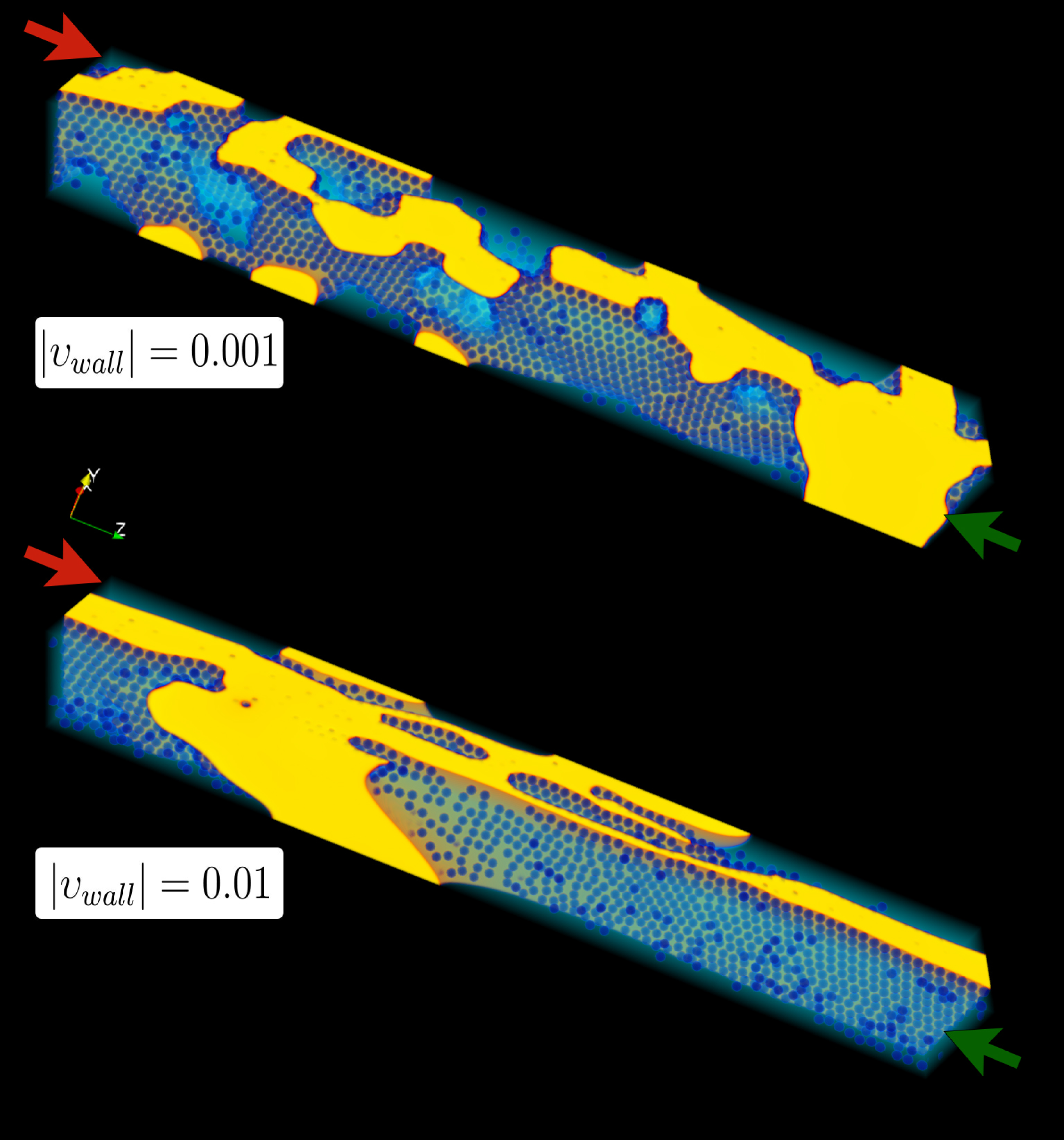
Figure 7: From top to bottom, two snapshots of the system undergo a shear rate, $|\upsilon_{wall}|$, of values $0.001$ and $0.01$, respectively. Both the images were collected after 400000 steps of time integration.

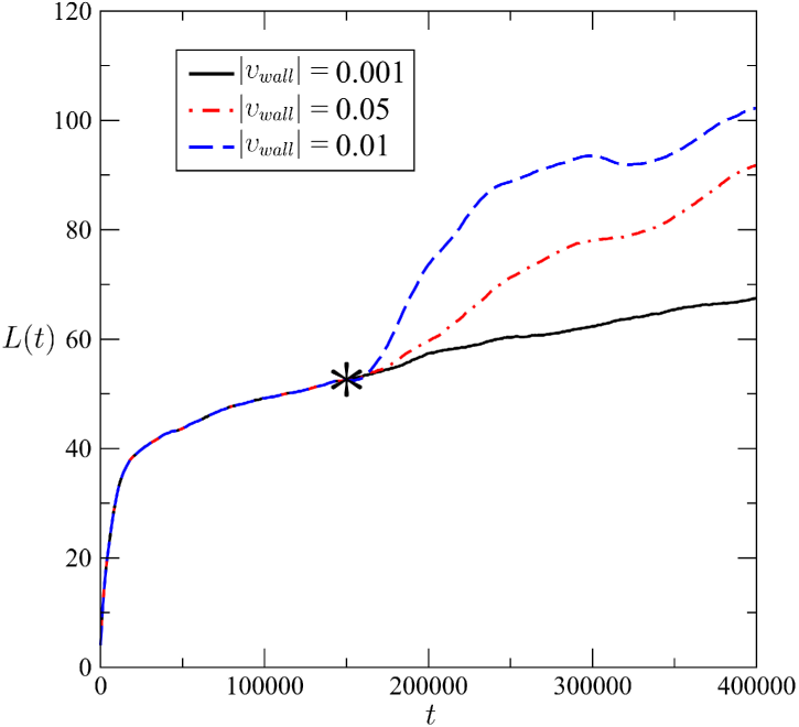
Figure 8: Average domain size over time for an orthogonal box of sides 128, 128, and 1024 at 15% in particle volume fraction. After a rapid growth of the domain size to over the initial 150000 time steps of equilibration, the system undergoes three different conditions of shear rate: $|\upsilon_{wall}|=0.001$, $0.05$, and $0.01$. The star symbol denotes the moment as the shear rate is applied on the bijel.

LBsoft opens up the opportunity to investigate the rheology of bijels not only in terms of bulk properties, but also under confinement. Leaving a detailed investigation to future publications, in the following we just wish to convey the flavor of the possibilities offered by the code. In particular, we report preliminary results of confined bijels under different conditions of shear rate.

This framework is of utmost importance not only as a fundamental non-equilibrium process, but also in view of numerous practical applications in material science, manufacturing, food processing, to name but a few. As an example, a better control of the bijel formation process in microfluidic devices would greatly benefit the rational design of the new bijel-based materials. Particularly notable is the case of 3D printing, where the possible application of the direct-write printing technique with bijels requires an in-depth knowledge of the effects of high shear rate as they occur in the micro-channels of the printing head.

The simulation setup discussed here involves an orthogonal box of sides $128\times 128\times 1024$ along the three Cartesian axes $x$, $y$, and $z$, respectively. The system is periodic along the $z$-axis (mainstream direction), while it is confined along the $x$ and $y$ directions. In particular, the two walls perpendicular to the $x$-axis move at a constant velocity,$|\upsilon_{wall}|$, oriented along the $z$-axis, with opposite directions (see Fig. 7). The walls perpendicular to the $y$-axis are set to no-slip boundary conditions.

The box is filled by two fluids, randomly distributed with initial fluid densities extracted from a Gaussian distribution of mean and standard deviation $1.0$ and $0.004$ lattice units, respectively. Colloidal spheres of radius $5.5$ are randomly distributed in the box, corresponding to a particle volume fraction of $0.15\%$. The system is initially equilibrated for $150,000$ timesteps, in order to attain the bijel formation. Subsequently, three different shear rates, $|\upsilon_{wall}|=0.001,0.005,0.01$ respectively, are applied to the system.

In the absence of shear and confinement, it is well known that the effect of colloids is to segregate around the interface, thereby slowing down and even arresting the coarse-graining of the binary mixture. This has far-reaching consequences on the mechanical and rheological properties of the corresponding materials. The application of a shear rate at the confining walls is expected to break up the fluid domains, thereby reviving the coarse-graining process against the blocking action of the colloids. This is exactly what the simulations show, as reported Fig. 7, which portrays two snapshots of the confined bijel configurations after $40,000$ timesteps.

In more quantitative terms, Fig. 8 reports the average domain size $L(t)$ for the three cases $|\upsilon_{wall}|=0.001,0.005,0.01$, as a function of time. As one can appreciate, the smallest shear leaves the coarsening process basically unaffected, while for $|\upsilon_{wall}|=0.005,0.01$, coarsening is clearly revived.

Many directions for future investigations can be envisaged: among others, i) a systematic study of the rheology of bijels under confinement, ii) the rheological behaviour under cyclic shear applications (hysteresis), iii) the inclusion of electrostatic interactions for the design of new materials based on polar bijels.

It hoped and expected that LBsoft may provide a valuable tool for the efficient exploration of the aforementioned topics and for the computational designed of bijel-like based materials in general.

6 Conclusion

We have presented LBsoft, an open-source software specifically aimed at numerical simulations of colloidal systems. LBsoft is implemented in FORTRAN programming language and permits to simulate large system sizes exploiting efficient parallel implementation. In particular, the strong scaling behaviour of the code shows that LBsoft delivers an excellent parallelization of the lattice-Boltzmann algorithm. Further, whenever the particle integrator is combined with the fluid solver, LBsoft continues to show a good performance in terms of scalability in both system size and number of processing cores.

In this work, the basic structure of LBsoft is reported along with the main guidelines of the actual implementation. Furthermore, several examples have been reported in order to convey to the reader a flavor of the typical problems which can be dealt with using LBsoft. In particular, the simulations of bi-jel systems demonstrate the capabilities of the present code to reproduce the complex dynamics of the particles trapped at the jammed layers in a rapid de-mixing emulsion.

The LBsoft code is open source and completely accessible on the public GitHub repository. This is in line with the spirit of open source software, namely to promote the contribution of independent developers to the user community.

7 Acknowledgments

We would like to thank Prof. Anthony Ladd for illuminating discussions on rigid body models and precious suggestions on their implementations. The software development process has received funding from the European Research Council under the European Union’s Horizon 2020 programme /ERC Grant Agreement n.739964 “COPMAT". ML acknowledges the project “3D-Phys" (PRIN 2017PHRM8X) from MIUR.

Appendix A Directives of input file

directive in system room:	meaning:
box $i_{1}$ $i_{2}$ $i_{3}$	dimension of the simulation box along the Cartesian axes
bound cond $i_{1}$ $i_{2}$ $i_{3}$	set boundary conditions along the Cartesian axes (0=wall,1=periodic)
close time $f$	Set job closure time to $f$ seconds
diagnostic yes	active the print of times measured in several subroutines of LBsoft code
decompos type $i$	type of domain decomposition fo parallel jobs
decompos dimen $i_{1}$ $i_{2}$ $i_{3}$	domain decomposition along the Cartesian axes
job time $f$	Set job time to $f$ seconds
print list $s_{1}\,\ldots$	print on terminal statistical data as indicated by symbolic strings
print list every $i$	print on terminal statistical data every $i$ steps
print binary yes	activate the raw data print in binary format
print binary every $i$	print raw data in binary file format every $i$ steps (default: 100)
print vtk yes	activate the output print in vtk files format
print vtk every $i$	print the output in vtk files format every $i$ steps
print vtk list $s_{1}\,\ldots$	print on vtk files the data indicated by symbolic strings
print xyz yes	activate the particle print in XYZ file format
print xyz every $i$	print particle positions in XYZ file format every $i$ steps (default: 100)
restart yes	restart LBsoft from a previous job
restart every $i$	print the restart files every $i$ steps (default: 10000)
seed $i$	seed control to the internal random number generator
steps $i$	number of time integration steps equal to $i$
test yes	activate an hash function for a deterministic initialization of LBsoft
directive in LB room:	meaning:
bound open east type $i$	type of open boundary on east wall
	(1=Dirichlet,2=Neumann,3=Equilibrium)
bound open west type $i$	type of open boundary on west wall
bound open front type $i$	type of open boundary on front wall
bound open rear type $i$	type of open boundary on rear wall
bound open north type $i$	type of open boundary on north wall
bound open south type $i$	type of open boundary on south wall
bound open east dens $f_{1}$ $f_{2}$	density of open boundary on east wall
bound open west dens $f_{1}$ $f_{2}$	density of open boundary on west wall
bound open front dens $f_{1}$ $f_{2}$	density of open boundary on front wall
bound open rear dens $f_{1}$ $f_{2}$	density of open boundary on rear wall
bound open north dens $f_{1}$ $f_{2}$	density of open boundary on north wall
bound open south dens $f_{1}$ $f_{2}$	density of open boundary on south wall
bound open east veloc $f_{1}$ $f_{2}$ $f_{3}$	velocity vector of open boundary on east wall
bound open west veloc $f_{1}$ $f_{2}$ $f_{3}$	velocity vector of open boundary on west wall
bound open front veloc $f_{1}$ $f_{2}$ $f_{3}$	velocity vector of open boundary on front wall
bound open rear veloc $f_{1}$ $f_{2}$ $f_{3}$	velocity vector of open boundary on rear wall
bound open north veloc $f_{1}$ $f_{2}$ $f_{3}$	velocity vector of open boundary on north wall
bound open south veloc $f_{1}$ $f_{2}$ $f_{3}$	velocity vector of open boundary on south wall
component $i$	number of fluid components equal to $i$
dens mean $f_{1}$ $f_{2}$	mean values of the initial fluid densities
dens stdev $f_{1}$ $f_{2}$	standard deviation values of the initial fluid densities
dens back $f_{1}$ $f_{2}$	background values of the initial fluid densities
dens rescal $i$ $f$	rescale the mass density every $i$ steps if deviating of $f$
	from the initial value taken as a reference point
dens ortho $i$ $f_{n}:n\in[1,\dots,8]$	orthogonal object numbered $i$ with extremes $f_{n}:n\in[1,\dots,6]$ and
	densities $f_{7}$ and $f_{8}$ in the box
dens sphere $i$ $f_{n}:n\in[1,\dots,7]$	spherical object numbered $i$ with center $f_{n}:n\in[1,\dots,3]$,
	radius and width $f_{4}$ and $f_{5}$ and densities $f_{6}$ and $f_{7}$
dens gauss	set a gaussian distribution of the initial fluid densities
dens uniform	set an uniform distribution of the initial fluid densities
dens special	set a special definition of the initial fluid densities by
	a set of objects defined in input file
force ext $f_{1}$ $f_{2}$ $f_{3}$	external force along the Cartesian axes
force shanc pair $f$	coupling constant of Shan-Chen force between the fluids
force cap $f$	set a capping value for the total force terms
veloc mean $f_{1}$ $f_{2}$ $f_{3}$	mean initial fluid velocities along the Cartesian axes
visc $f_{1}$ $f_{2}$	viscosity of the fluids
tau $f_{1}$ $f_{2}$	relaxation time of the fluids for the BGK collisional
wetting mode $i$ $f_{1}$ $f_{2}$	model of wetting wall and respective constants
	(0=averaged density,1=constant density)
directive in MD room:	meaning:
delr $f$	set Verlet neighbour list shell width to $f$
densvar $f$	density variation for particle arrays
field pair wca $i_{1}$ $i_{2}$ $f_{1}$ $f_{2}$	pair of particle types, force constant and
	minimum distance of the Weeks-Chandler-Andersen potential
field pair lj $i_{1}$ $i_{2}$ $f_{1}$ $f_{2}$	pair of particle types, force constant and
	minimum distance of the Lennard-Jones potential
field pair hz $i_{1}$ $i_{2}$ $f_{1}$ $f_{2}$	pair of particle types, force constant,
	minimum distance and capping distance of the Hertzian potential
force ext $f_{1}$ $f_{2}$ $f_{3}$	external particle force along the Cartesian axes
force shanc angle $f_{1}$ $f_{2}$	inflection and width of the switching function
	tuning the particle wettability
force shanc part $f_{1}$ $f_{2}$	constants of wetting wall on particles
force cap $f$	set a capping value for the total particle force terms
lubric yes $f_{1}$ $f_{2}$ $f_{3}$	activate lubrication force with rescaling constant,
	minimum distance and capping distance
init temperat $f$	amplitude of Maxwell distribution of initial particle velocity
mass $i$ $f$	set mass $f$ to the particle of type $i$
moment fix $i$	remove the linear momentum every $i$ steps
particle yes	activate the particle part of LBsoft
particle type $i$ $s$ $\dots$	number of particle types labelled by symbolic strings
rcut $f$	set required forces cutoff to $f$
rotate yes	activate the rotation of the particles
rotate yes	activate the rotation of the particles
side wall const $f$	constant of soft harmonic wall
side wall dist $f$	location of the minimum of soft harmonic wall
torque ext $f_{1}$ $f_{2}$ $f_{3}$	external particle torque along the Cartesian axes

Table 4: Here, we report the list of directives available in LBsoft. Note $i$, $f$, and $s$ denote an integer number, a floating point number, and a string, respectively. Note that the input parameters should be expresses in lattice units.

Appendix B List of keys of input particle file

keys:	meaning:
mass	mass of the particle
vx	particle velocity along x
vy	particle velocity along y
vz	particle velocity along z
ox	particle angular velocity along x
oy	particle angular velocity along y
oz	particle angular velocity along z
rad	radius of the spherical particle
radx	radius of the particle along x
rady	radius of the particle along y
radz	radius of the particle along z

Table 5: List of symbolic string keys is reported with their corresponding meanings for the particles input file named input.xyz.

Appendix C List of keys of output observables

keys:	meaning:
t	time
dens1	mean fluid density of first component
dens2	mean fluid density of second component
maxd1	max fluid density of first component
maxd2	max fluid density of second component
mind1	min fluid density of first component
mind2	min fluid density of second component
maxvx	max fluid velocity of fluid mix along x
minvx	min fluid velocity of fluid mix along x
maxvy	max fluid velocity of fluid mix along y
minvy	min fluid velocity of fluid mix along y
maxvz	max fluid velocity of fluid mix along z
minvz	min fluid velocity of fluid mix along z
fvx	mean fluid velocity along x
fvy	mean fluid velocity along y
fvz	mean fluid velocity along z
engkf	kinetic energy of fluid
engke	kinetic energy of particle
engcf	configuration energy
engrt	rotational energy
engto	total energy
intph	fluid interphase volume fraction
rminp	min pair distance between particles
tempp	particle temperature as ratio of KbT
maxpv	max particle velocity
pvm	mean particle velocity module
pvx	mean particle velocity along x
pvy	mean particle velocity along y
pvz	mean particle velocity along z
pfm	mean particle force module
pfx	mean particle force along x
pfy	mean particle force along y
pfz	mean particle force along z
cpu	time for every print interval in seconds
cpur	remaining time to the end in seconds
cpue	elapsed time in seconds

Table 6: In LBsoft a set of instantaneous and statistical data are available to be printed by selecting the corresponding key. Here, the list of symbolic string keys is reported with their corresponding meanings. All the quantities must be expressed in lattice units, if not explicitly declared in Table.

Appendix D Benchmark input files

Benchmark test 1. Input file of single fluid test.
[ROOM SYSTEM]
box 512 512 512
steps 5000
boundary condition 1 1 1
decomposition type 7
print list maxd1 mind1 maxvx maxvy maxvz
print every 10
test yes
[END ROOM]
[ROOM LB]
components 1
density gaussian
density mean 1.0
density stdev 1.d-4
velocity mean 0.d0
fluid tau 1.d0
[END ROOM]
[END]

Benchmark test 2. Input file of two fluid test.
[ROOM SYSTEM]
box 512 512 512
steps 5000
boundary condition 1 1 1
decomposition type 7
print list maxd1 mind1 maxvx maxvy maxvz
print every 10
test yes
[END ROOM]
[ROOM LB]
components 2
density gaussian
density mean 1.0 1.0
density stdev 1.d-4 1.d-4
velocity mean 0.d0 0.d0
fluid tau 1.d0 1.d0
force shanchen pair 0.65d0
[END ROOM]
[END]

Benchmark test 3. Input file of bi-jel test.
[ROOM SYSTEM]
box 512 512 512
steps 5000
boundary condition 1 1 1
decomposition type 7
print list maxd1 mind1 maxvx maxvy maxvz
print every 10
test yes
[END ROOM]
[ROOM LB]
components 2
density gaussian
density mean 1.0 1.0
density stdev 1.d-4 1.d-4
velocity mean 0.d0 0.d0
fluid tau 1.d0 1.d0
force shanchen pair 0.65d0
[END ROOM]
[ROOM MD]
particle yes
particle type 1
C
rotate yes
lubric yes 0.1d0 0.67d0 0.5d0
densvar 5.d0
rcut 12.d0
delr 1.0d0
shape spherical 1 5.5d0
field pair hz 1 1 20.d0 12.d0 11.d0
mass 1 472.d0
initial temperature 0.0
force shanchen angle 108.d0 10.d0
force shanchen particel 0.1d0 0.1d0
[END ROOM]
[END]

References

- [1] A. Fernandez-Nieves, A. M. Puertas, Fluids, Colloids and Soft Materials: An Introduction to Soft Matter Physics, Vol. 7, John Wiley & Sons, 2016.
- [2] R. Piazza, Soft matter: the stuff that dreams are made of, Springer Science & Business Media, 2011.
- [3] R. Mezzenga, P. Schurtenberger, A. Burbidge, M. Michel, Understanding foods as soft materials, Nature materials 4 (10) (2005) 729.
- [4] A. J. Ladd, Lattice-boltzmann methods for suspensions of solid particles, Molecular Physics 113 (17-18) (2015) 2531–2537.
- [5] A. Ladd, R. Verberg, Lattice-boltzmann simulations of particle-fluid suspensions, Journal of statistical physics 104 (5-6) (2001) 1191–1251.
- [6] C. K. Aidun, Y. Lu, E.-J. Ding, Direct analysis of particulate suspensions with inertia using the discrete boltzmann equation, Journal of Fluid Mechanics 373 (1998) 287–311.
- [7] A. J. Ladd, Numerical simulations of particulate suspensions via a discretized boltzmann equation. part 1. theoretical foundation, Journal of fluid mechanics 271 (1994) 285–309.
- [8] S. U. Pickering, Cxcvi.-emulsions, Journal of the Chemical Society, Transactions 91 (1907) 2001–2021.
- [9] Q. Xie, G. B. Davies, J. Harting, Direct assembly of magnetic janus particles at a droplet interface, ACS nano 11 (11) (2017) 11232–11239.
- [10] H. Liu, Q. Kang, C. R. Leonardi, S. Schmieschek, A. Narváez, B. D. Jones, J. R. Williams, A. J. Valocchi, J. Harting, Multiphase lattice boltzmann simulations for porous media applications, Computational Geosciences 20 (4) (2016) 777–805.
- [11] S. Frijters, F. Günther, J. Harting, Effects of nanoparticles and surfactant on droplets in shear flow, Soft Matter 8 (24) (2012) 6542–6556.
- [12] F. Jansen, J. Harting, From bijels to pickering emulsions: A lattice boltzmann study, Physical Review E 83 (4) (2011) 046707.
- [13] V. Heuveline, J. Latt, The openlb project: an open source and object oriented implementation of lattice boltzmann methods, International Journal of Modern Physics C 18 (04) (2007) 627–634.
- [14] M. A. Seaton, R. L. Anderson, S. Metz, W. Smith, Dl_meso: highly scalable mesoscale simulations, Molecular Simulation 39 (10) (2013) 796–821.
- [15] M. Bauer, S. Eibl, C. Godenschwager, N. Kohl, M. Kuron, C. Rettinger, F. Schornbaum, C. Schwarzmeier, D. Thönnes, H. Köstler, et al., walberla: A block-structured high-performance framework for multiphysics simulations, Computers & Mathematics with Applications.
- [16] F. Schornbaum, U. Rude, Massively parallel algorithms for the lattice boltzmann method on nonuniform grids, SIAM Journal on Scientific Computing 38 (2) (2016) C96–C126.
- [17] J. Latt, et al., Palabos, parallel lattice boltzmann solver, FlowKit, Lausanne, Switzerland.
- [18] J.-C. Desplat, I. Pagonabarraga, P. Bladon, Ludwig: A parallel lattice-boltzmann code for complex fluids, Computer Physics Communications 134 (3) (2001) 273–290.
- [19] M. D. Mazzeo, P. V. Coveney, Hemelb: A high performance parallel lattice-boltzmann code for large scale fluid flow in complex geometries, Computer Physics Communications 178 (12) (2008) 894–914.
- [20] D. M. Holman, R. M. Brionnaud, Z. Abiza, Solution to industry benchmark problems with the lattice-boltzmann code xflow, in: Proceeding in the European Congress on Computational Methods in Applied Sciences and Engineering (ECCOMAS), 2012.
- [21] D. P. Lockard, L.-S. Luo, S. D. Milder, B. A. Singer, Evaluation of powerflow for aerodynamic applications, Journal of Statistical Physics 107 (1-2) (2002) 423–478.
- [22] T. Krüger, H. Kusumaatmaja, A. Kuzmin, O. Shardt, G. Silva, E. M. Viggen, The lattice boltzmann method, Springer International Publishing 10 (2017) 978–3.
- [23] S. Succi, S. Succi, The Lattice Boltzmann Equation: For Complex States of Flowing Matter, Oxford University Press, 2018.
- [24] A. J. Ladd, Numerical simulations of particulate suspensions via a discretized boltzmann equation. part 2. numerical results, Journal of fluid mechanics 271 (1994) 311–339.
- [25] I. Ginzburg, F. Verhaeghe, D. d’Humieres, Two-relaxation-time lattice boltzmann scheme: About parametrization, velocity, pressure and mixed boundary conditions, Communications in computational physics 3 (2) (2008) 427–478.
- [26] M. Sbragaglia, R. Benzi, L. Biferale, S. Succi, F. Toschi, Surface roughness-hydrophobicity coupling in microchannel and nanochannel flows, Physical review letters 97 (20) (2006) 204503.
- [27] J. Onishi, A. Kawasaki, Y. Chen, H. Ohashi, Lattice boltzmann simulation of capillary interactions among colloidal particles, Computers & Mathematics with Applications 55 (7) (2008) 1541–1553.
- [28] H. Hertz, About the contact of elastic solid bodies (über die berührung fester elastischer körper), J Reine Angew Math 5 (1881) 12–23.
- [29] N.-Q. Nguyen, A. Ladd, Lubrication corrections for lattice-boltzmann simulations of particle suspensions, Physical Review E 66 (4) (2002) 046708.
- [30] S. L. Altmann, Rotations, quaternions, and double groups, Courier Corporation, 2005.
- [31] M. Svanberg, An improved leap-frog rotational algorithm, Molecular physics 92 (6) (1997) 1085–1088.
- [32] J. Racine, The cygwin tools: a gnu toolkit for windows, Journal of Applied Econometrics 15 (3) (2000) 331–341.
- [33] T. Pohl, M. Kowarschik, J. Wilke, K. Iglberger, U. Rüde, Optimization and profiling of the cache performance of parallel lattice boltzmann codes, Parallel Processing Letters 13 (04) (2003) 549–560.
- [34] K. Mattila, J. Hyväluoma, J. Timonen, T. Rossi, Comparison of implementations of the lattice-boltzmann method, Computers & Mathematics with Applications 55 (7) (2008) 1514–1524.
- [35] M. Wittmann, T. Zeiser, G. Hager, G. Wellein, Comparison of different propagation steps for lattice boltzmann methods, Computers & Mathematics with Applications 65 (6) (2013) 924–935.
- [36] S. Succi, G. Amati, M. Bernaschi, G. Falcucci, M. Lauricella, A. Montessori, Towards exascale lattice boltzmann computing, Computers & Fluids.
- [37] D. Fincham, Leapfrog rotational algorithms, Molecular Simulation 8 (3-5) (1992) 165–178.
- [38] D. Rozmanov, P. G. Kusalik, Robust rotational-velocity-verlet integration methods, Physical Review E 81 (5) (2010) 056706.
- [39] D. Frenkel, B. Smit, Understanding molecular simulation: from algorithms to applications, Vol. 1, Academic Press, London, UK, 2001.
- [40] R. W. Hockney, J. W. Eastwood, Computer simulation using particles, CRC Press, Boca Raton, USA, 1988.
- [41] D. Auerbach, W. Paul, A. Bakker, C. Lutz, W. Rudge, F. F. Abraham, A special purpose parallel computer for molecular dynamics: Motivation, design, implementation, and application, Journal of Physical Chemistry 91 (19) (1987) 4881–4890.
- [42] F. Darema, The spmd model: Past, present and future, in: European Parallel Virtual Machine/Message Passing Interface Users’ Group Meeting, Springer, 2001, pp. 1–1.
- [43] W. D. Gropp, Parallel computing and domain decomposition, in: Fifth International Symposium on Domain Decomposition Methods for Partial Differential Equations, Philadelphia, PA, 1992, pp. 349–361.
- [44] W. Smith, Molecular dynamics on hypercube parallel computers, Computer Physics Communications 62 (2-3) (1991) 229–248.
- [45] W. Smith, Molecular dynamics on distributed memory (mimd) parallel computers, Theoretica chimica acta 84 (4-5) (1993) 385–398.
- [46] M. Pinches, D. Tildesley, W. Smith, Large scale molecular dynamics on parallel computers using the link-cell algorithm, Molecular Simulation 6 (1-3) (1991) 51–87.
- [47] D. Rapaport, Multi-million particle molecular dynamics: Ii. design considerations for distributed processing, Computer Physics Communications 62 (2-3) (1991) 217–228.
- [48] W. J. Schroeder, B. Lorensen, K. Martin, The visualization toolkit: an object-oriented approach to 3D graphics, Kitware, New York, USA, 2004.
- [49] U. Ayachit, The paraview guide: a parallel visualization application, Kitware, New York, USA, 2015.
- [50] W. Humphrey, A. Dalke, K. Schulten, Vmd: visual molecular dynamics, Journal of molecular graphics 14 (1) (1996) 33–38.
- [51] S. Schmieschek, L. Shamardin, S. Frijters, T. Krüger, U. D. Schiller, J. Harting, P. V. Coveney, Lb3d: A parallel implementation of the lattice-boltzmann method for simulation of interacting amphiphilic fluids, Computer Physics Communications 217 (2017) 149–161.
- [52] E. Herzig, K. White, A. Schofield, W. Poon, P. Clegg, Bicontinuous emulsions stabilized solely by colloidal particles, Nature materials 6 (12) (2007) 966.
- [53] M. E. Cates, P. S. Clegg, Bijels: a new class of soft materials, Soft Matter 4 (11) (2008) 2132–2138.
- [54] J. Harting, G. Giupponi, P. V. Coveney, Structural transitions and arrest of domain growth in sheared binary immiscible fluids and microemulsions, Physical Review E 75 (4) (2007) 041504.
- [55] A. Tiribocchi, A. Piscitelli, G. Gonnella, A. Lamura, Pattern study of thermal phase separation for binary fluid mixtures, International Journal of Numerical Methods for Heat & Fluid Flow 21 (5) (2011) 572–583.
- [56] V. M. Kendon, M. E. Cates, I. Pagonabarraga, J.-C. Desplat, P. Bladon, Inertial effects in three-dimensional spinodal decomposition of a symmetric binary fluid mixture: a lattice boltzmann study, Journal of Fluid Mechanics 440 (2001) 147–203.
- [57] M. Laradji, S. Toxvaerd, O. G. Mouritsen, Molecular dynamics simulation of spinodal decomposition in three-dimensional binary fluids, Physical review letters 77 (11) (1996) 2253.
- [58] K. Stratford, R. Adhikari, I. Pagonabarraga, J.-C. Desplat, M. E. Cates, Colloidal jamming at interfaces: A route to fluid-bicontinuous gels, Science 309 (5744) (2005) 2198–2201.
- [59] S. Plimpton, Fast parallel algorithms for short-range molecular dynamics, Journal of computational physics 117 (1) (1995) 1–19.
- [60] I. T. Todorov, W. Smith, K. Trachenko, M. T. Dove, Dl_poly_3: new dimensions in molecular dynamics simulations via massive parallelism, Journal of Materials Chemistry 16 (20) (2006) 1911–1918.
-
[61]
P. Steve, Lammps benchmarks,
online; accessed 14-October-2019 (2016).
URL http://lammps.sandia.gov/bench.html/ - [62] S. Jarvis, S. Wright, S. Hammond, High Performance Computing Systems. Performance Modeling, Benchmarking, and Simulation: 8th International Workshop, PMBS 2017, Denver, CO, USA, November 13, 2017, Proceedings, Vol. 10724, Springer, 2017.