Large Steklov eigenvalues via homogenisation on manifolds

Abstract.

Using methods in the spirit of deterministic homogenisation theory we obtain convergence of the Steklov eigenvalues of a sequence of domains in a Riemannian manifold to weighted Laplace eigenvalues of that manifold. The domains are obtained by removing small geodesic balls that are asymptotically densely uniformly distributed as their radius tends to zero. We use this relationship to construct manifolds that have large Steklov eigenvalues.

In dimension two, and with constant weight equal to $1$, we prove that Kokarev’s upper bound of $8\pi$ for the first nonzero normalised Steklov eigenvalue on orientable surfaces of genus 0 is saturated. For other topological types and eigenvalue indices, we also obtain lower bounds on the best upper bound for the eigenvalue in terms of Laplace maximisers. For the first two eigenvalues, these lower bounds become equalities. A surprising consequence is the existence of free boundary minimal surfaces immersed in the unit ball by first Steklov eigenfunctions and with area strictly larger than $2\pi$. This was previously thought to be impossible. We provide numerical evidence that some of the already known examples of free boundary minimal surfaces have these properties and also exhibit simulations of new free boundary minimal surfaces of genus zero in the unit ball with even larger area. We prove that the first nonzero Steklov eigenvalue of all these examples is equal to 1, as a consequence of their symmetries and topology, so that they verify a general conjecture by Fraser and Li.

In dimension three and larger, we prove that the isoperimetric inequality of Colbois–El Soufi–Girouard is sharp and implies an upper bound for weighted Laplace eigenvalues. We also show that in any manifold with a fixed metric, one can construct by varying the weight a domain with connected boundary whose first nonzero normalised Steklov eigenvalue is arbitrarily large.

1. Introduction and main results

1.1. The Laplace and Steklov eigenvalue problems

Let $(M,g)$ be a smooth, closed connected Riemannian manifold of dimension $d\geq 2$ and let $\Omega\subset M$ be a domain with smooth boundary $\partial\Omega$. Let $\beta\in\mathrm{C}^{\infty}(M)$ be a smooth positive function. We study the weighted Laplace eigenvalue problem

$$-\Delta\varphi=\lambda\beta\varphi\qquad\text{in }M$$ (1)

and the Steklov eigenvalue problem

$$\begin{cases}\Delta u=0&\text{in }\Omega;\\ \partial_{\nu}u=\sigma u&\text{on }\partial\Omega;\end{cases}$$ (2)

where $\Delta$ is the Laplace operator and $\nu$ is the outwards unit normal. The spectra of the Laplace and Steklov problems are discrete and their eigenvalues form sequences

$$0=\lambda_{0}<\lambda_{1}(M,g,\beta)\leq\lambda_{2}(M,g,\beta)\leq\dotso\nearrow\infty$$ (3)

and

$$0=\sigma_{0}<\sigma_{1}(\Omega,g)\leq\sigma_{2}(\Omega,g)\leq\dotso\nearrow\infty$$ (4)

accumulating only at infinity. Problem (1) is a staple of geometric spectral theory, see e.g. [2, 8]. The eigenvalues $\lambda_{k}(M,g,\beta)$ correspond to natural frequencies of a membrane that is non-homogeneous when $\beta$ is not constant. It has recently been studied by Colbois–El Soufi [15] and Colbois–El Soufi–Savo [17] in the Riemannian setting. Problem (2) is a classical problem originating in mathematical physics [66] and which has received growing attention in the last few years. Its eigenvalues are those of the Dirichlet-to-Neumann operator, which maps a function $f$ on $\partial\Omega$ to the normal derivative on the boundary of its harmonic extension. See [35] for a survey.

Our main theorem states that for any positive $\beta\in\mathrm{C}^{\infty}(M)$, Problem (1) may be realized as a limit of Problem (2) defined on carefully constructed domains $\Omega^{\varepsilon}\subset M$. Denote by $\,\mathrm{d}\mu_{g}$ the Lebesgue measure on $M$ and for every domain $\Omega\subset M$ by $\,\mathrm{d}A_{\partial\Omega}$ the measure on $M$ defined by integration against the Hausdorff measure on $\partial\Omega$.

Theorem 1.1.

Let $(M,g)$ be a closed Riemannian manifold, and $\beta\in\mathrm{C}^{\infty}(M)$ positive. There is a sequence of domains $\Omega^{\varepsilon}\subset M$ such that $\,\mathrm{d}A_{\partial\Omega^{\varepsilon}}$ converges weak-$*$ to $\beta\,\mathrm{d}\mu_{g}$ and

$$\sigma_{k}(\Omega^{\varepsilon},g)\xrightarrow{\varepsilon\to 0}\lambda_{k}(M,g,\beta).$$ (5)

The proof of Theorem 1.1 is in the spirit of Girouard–Henrot–Lagacé [34] where Neumann eigenvalues of a domain in Euclidean space are related to Steklov eigenvalues of subdomains through periodic homogenisation by obstacles.

Homogenisation theory is a branch of applied mathematics that is interested in the study of PDEs and variational problems in the presence of structures at many different scales; in the presence of two scales they are usually referred to as the macrostructure and microstructure. The methods are usually divided in two general categories: deterministic (or periodic), and stochastic. The effectiveness of homogenisation in shape optimisation, see for example the Allaire’s influencial monograph [1] and the references therein, leads one to believe that it should also be useful elsewhere in geometric analysis.

The main obstacle to the application of deterministic homogenisation theory in the Riemannian setting is that most Riemannian manifolds do not exhibit any form of periodic structure. It is therefore not surprising that homogenisation theory in this setting has either been applied when an underlying manifold exhibits a periodic-like structure, see e.g. the work of Boutet de Monvel–Khruslov [3] and Contreras–Iturriaga–Siconolfi [22], or used the periodic structure of an ambient space in which a manifold is embedded, see Braides–Cancedda–Chiadò Piat [4] or relied on an imposed periodic structure in predetermined charts, see Dobberschütz–Böhm [24]. Our approach is distinct in that it is entirely intrinsic and does not require a periodic structure at any stage.

We note that stochastic homogenisation has been used in geometric contexts, see e.g. the recent paper by Li [57]. Chavel–Feldman [9, 10] also studied the effect on the spectrum of the Laplacian of removing a large, but fixed, number of small geodesic balls on which Dirichlet boundary conditions are imposed. However, no consideration was given to the distribution of those geodesic balls, nor to asymptotic behaviour joint in the number of balls removed and their size.

Remark 1.2.

It is natural to expect that the Steklov eigenvalues of a domain $\Omega$ with smooth boundary would be related to the eigenvalues $\lambda_{k}(\partial\Omega)$ of the Laplace operator of its boundary, since the Dirichlet-to-Neumann map is an elliptic pseudo-differential operator that has the same principal symbol as the square root of the Laplace operator on $\partial\Omega$, see [67, Section 7.11]. Indeed, upper bounds for $\sigma_{k}(\Omega)$ in terms of $\lambda_{k}(\partial\Omega)$ have been obtained by Wang–Xia [69] for $k=1$ and by Karpukhin [45] for higher eigenvalues. Quantitative estimate for $|\sigma_{k}(\Omega)-\sqrt{\lambda_{k}(\partial\Omega)}|$ have been obtained by Provenzano–Stubbe [62] for domains in Euclidean space and by Xiong [70] and Colbois–Girouard–Hassannezhad [19] in the Riemannian setting. The eigenvalues of various other spectral problems have also been compared with Steklov eigenvalues. See the work of Kuttler–Sigillito [52] and Hassannezhad–Siffert [38].

A different type of relationship was studied in Lamberti–Provenzano [54], where it is proved that the Steklov eigenvalues of a domain $\Omega\subset\mathbb{R}^{d}$ can be obtained as appropriate limits of non-homogeneous Neumann eigenvalues with the mass concentrated at the boundary of $\Omega$.

1.2. Isoperimetric inequalities

Theorem 1.1 has several applications to the study of isoperimetric inequalities for Steklov eigenvalues. These are most naturally stated in terms of the scale invariant eigenvalues

$$\Lambda_{k}(M,g):=\operatorname{Vol}_{g}(M)^{2/d}\lambda_{k}(M,g,1)$$ (6)

and

$$\Sigma_{k}(\Omega,g):=\mathcal{H}^{d-1}(\partial\Omega)^{1/(d-1)}\sigma_{k}(\Omega,g),$$ (7)

where $\operatorname{Vol}_{g}(M)$ is the volume of $M$ and $\mathcal{H}^{d-1}(\partial\Omega)$ is the $(d-1)$-Hausdorff measure of the boundary $\partial\Omega$. It is natural to ask for upper bounds on the functionals (6) and (7), and as such to define

$$\Lambda_{k}^{*}(M):=\sup_{g\in\mathcal{G}(M)}\Lambda_{k}(M,g)$$ (8)

and

$$\Sigma_{k}^{*}(M):=\sup_{\Omega\subset M}\sup_{g\in\mathcal{G}(\overline{\Omega})}\Sigma_{k}(\Omega,g)$$ (9)

where for any manifold, with or without boundary, $\mathcal{G}(M)$ is the set of all Riemannian metrics on $M$. Spectral isoperimetric inequalities often have a wildly different behaviour in dimension two than in dimension at least three, as exhibited in the work of Colbois–Dodziuk [13] and Korevaar [51]. As such, we study these cases separately.

1.2.1. Isoperimetric inequalities in dimension two

From Colbois–El Soufi–Girouard [16] it is known that $\Sigma_{k}^{*}(M)$ is finite for each surface. The next result provides an effective lower bound.

Theorem 1.3.

For every $k\in\mathbb{N}$ and every smooth, closed, connected surface $M$,

$$\Sigma_{k}^{*}(M)\geq\Lambda_{k}^{*}(M).$$ (10)

This should be compared with [34, Theorem 9] where a similar inequality was proved, relating Steklov and Neumann eigenvalues of a domain in Euclidean space. The storied study of $\Lambda_{k}^{*}$ for various $k$ and smooth surfaces $M$ of different topologies yields explicit lower bounds for $\Sigma_{k}^{*}$, which we record in Section 7. Kokarev [50, Theorem $A_{1}$, Example 1.3] proved that $\Sigma_{1}^{*}(\mathbb{S}^{2})\leq 8\pi$. Theorem 1.3 and the known value $\lambda_{1}(\mathbb{S}^{2},g_{0})=2$ for the round sphere, shows that Kokarev’s bound is sharp.

Corollary 1.4.

The following equality holds:

$$\Sigma_{1}^{*}(\mathbb{S}^{2})=8\pi.$$ (11)

Remark 1.5.

Both Corollary 1.4 and, further along, Theorem 1.13 along with (21) are in contradiction with parts of [31, Theorems 8.2], where the bound

$$\Sigma_{1}^{*}(\mathbb{S}^{2})\leq 4\pi$$ (12)

is given. Further discussion and related results are delayed to Appendix A.

Very recent work of Karpukhin–Stern [47, Theorem 5.2] in fact shows that for all surfaces $M$, and for $j\in\left\{1,2\right\}$

$$\Sigma_{j}^{*}(M)\leq\Lambda_{j}^{*}(M),$$ (13)

using methods from min-max theory of harmonic maps. In combination with Theorem 1.3, we obtain the following result, also presented as [47, Proposition 5.9], which extends Corollary 1.4.

Corollary 1.6.

For all closed surfaces $M$, the following equalities hold

$$\Sigma_{1}^{*}(M)=\Lambda_{1}^{*}(M)$$ (14)

and

$$\Sigma_{2}^{*}(M)=\Lambda_{2}^{*}(M).$$ (15)

This leads naturally to the following conjecture.

Conjecture.

For all closed surfaces $M$ and all $k\in\mathbb{N}$,

$$\Sigma_{k}^{*}(M)=\Lambda_{k}^{*}(M).$$ (16)

1.2.2. Isoperimetric inequalities in dimension at least three

For $d\geq 3$, it follows from the work of Colbois–Dodziuk [13] that $\Lambda_{1}^{*}(M)=+\infty$. Together with Theorem 1.1 this gives $\Sigma_{1}^{*}(M)=+\infty$. Using the extra freedom provided by the weight $\beta$, we arrive at more precise statements, starting with the following corollary to Theorem 1.1.

Corollary 1.7.

Let $(M,g)$ be a Riemannian manifold of dimension $d\geq 2$. For constant density $\beta>0$, the domains $\Omega^{\varepsilon}\subset M$ obtained in Theorem 1.1 satisfy

$$\Sigma_{k}(\Omega^{\varepsilon},g)\xrightarrow{\varepsilon\to 0}\beta^{\frac{2-d}{d-1}}\operatorname{Vol}_{g}(M)^{\frac{2-d}{d(d-1)}}\Lambda_{k}(M,g).$$ (17)

This is a direct consequence of Theorem 1.1 since for constant density $\beta>0$ one has

$$\lambda_{k}(M,g,\beta)=\frac{1}{\beta}\lambda_{k}(M,g).$$

By removing thin tubes joining boundary components of a domain $\Omega\subset M$, Fraser–Schoen [32] proved that in dimension $d\geq 3$, there is a family of domains $\Omega_{\delta}\subset\Omega$, with connected boundary and such that $\left\lvert\Sigma_{1}(\Omega)-\Sigma_{1}(\Omega_{\delta})\right\rvert<\delta$. In combination with the previous corollary, this leads to the following result.

Corollary 1.8.

Let $(M,g)$ be a Riemannian manifold of dimension $d\geq 3$. Then there exists a sequence of domains $\Omega^{\varepsilon}\subset M$ with connected boundary such that

$$\lim_{\varepsilon\to 0}\Sigma_{1}(\Omega^{\varepsilon},g)=+\infty.$$ (18)

In recent years several constructions of manifolds with large normalised Steklov eigenvalue $\Sigma_{1}$ have been proposed. Colbois–Girouard [18] and Binoy [20] constructed a sequence $\Omega_{n}$ of compact surfaces with connected boundary such that $\Sigma_{1}(\Omega_{n})\to\infty$. Cianci–Girouard [11] proved that some manifolds $M$ of dimension $d\geq 4$ carry Riemannian metrics that are prescribed on $\partial M$ with uniformly bounded volume and arbitrarily large first Steklov eigenvalue $\sigma_{1}$. Corollary 1.8 provides a new outlook on this question.

1.2.3. Transferring bounds for Steklov eigenvalues to bounds for Laplace eigenvalues

If $(M,g)$ is conformally equivalent to a Riemannian manifold with non-negative Ricci curvature, it follows from Colbois–Girouard–El Soufi [16] that for each domain $\Omega\subset M$ with smooth boundary, and for each $k\geq 1$,

$$\sigma_{k}(\Omega)\leq C_{d}\frac{\operatorname{Vol}_{g}(\Omega)^{\frac{d-2}{d}}}{\mathcal{H}^{d-1}(\partial\Omega)}k^{2/d}.$$ (19)

Using the domains $\Omega^{\varepsilon}$ from Theorem 1.1 and taking the limit as $\varepsilon\to 0$ leads to the following.

Corollary 1.9.

Let $(M,g)$ be a closed manifold with $g$ conformally equivalent to a metric with nonnegative Ricci curvature. For each $\beta\in C^{\infty}(M)$ positive,

$$\lambda_{k}(M,g,\beta)\int_{M}\beta\,d\mu_{g}\leq C_{d}\operatorname{Vol}_{g}(M)^{\frac{d-2}{d}}k^{2/d}.$$ (20)

This is a special case of an inequality that was proved in Grigor’yan–Netrusov–Yau [36, Theorem 5.9].

Corollary 1.10.

The exponent  $2/d$ cannot be improved in (19), and the exponents on $\operatorname{Vol}_{g}(\Omega)$ and $\mathcal{H}^{d-1}(\partial\Omega)$ cannot be replaced by any other exponents.

Indeed for $\beta>0$ constant, inequality (20) becomes $\lambda_{k}(M,g)\operatorname{Vol}_{g}(M)^{\frac{2}{d}}\leq C_{d}k^{2/d}$, where the exponent carries over from (19). That it cannot be improved follows from the Weyl Law. Now, changing the exponent of $\mathcal{H}^{d-1}(\partial\Omega)$ in (19) would yield an inequality with a non-trivial exponent for $\beta$, while changing the exponent of $\operatorname{Vol}_{g}(\Omega)$ would lead to an inequality similar to (20), but not invariant under scaling of the Riemannian metric.

Remark 1.11.

Corollary 1.10 improves uppon [16, Remark 1.4], where it was already observed that the exponent $2/d$ could not be replaced by $1/(d-1)$ in inequality (19). Note also that for an Euclidean domain $\Omega\subset\mathbb{R}^{d}$, it follows from the isoperimetric inequality and (19) that $\sigma_{k}(\Omega)|\partial\Omega|^{1/(d-1)}\leq Ck^{2/d}$. Deciding if the exponent $2/d$ can be improved in this inequality is still an open problem, which was proposed as [35, Open problem 5].

1.3. Free boundary minimal surfaces

In dimension $d=2$, the striking connection between the Steklov eigenvalue problem and free boundary minimal submanifolds in the unit ball was revealed by Fraser and Schoen in [29, 30, 31].

Definition 1.12 (cf. [55, Theorem 2.2]).

For $m\geq 3$, let $\mathbb{B}^{m}$ be the $m$-dimensional Euclidean unit ball and let $\Omega\subset\mathbb{B}^{m}$ be a $k$-dimensional submanifold with boundary $\partial\Omega=\overline{\Omega}\cap\partial\mathbb{B}^{m}$. We say that $\Omega$ is a free boundary minimal submanifold in $\mathbb{B}^{m}$ if one of the following equivalent conditions hold.

1. $\Omega$ it is a critical point for the area functional among all $k$-dimensional submanifolds of $\mathbb{B}^{m}$ with boundary on $\partial\mathbb{B}^{m}$.

2. $\Omega$ has vanishing mean curvature and meets $\partial\mathbb{B}^{m}$ orthogonally.

3. The coordinate functions $x^{1},\dotsc,x^{m}$ restricted to $\Omega$ are solutions to the Steklov eigenvalue problem (2) with eigenvalue $\sigma=1$.

Conditions (1) and (2) can be used to generalise Definition 1.12 to arbitrary background manifolds in place of $\mathbb{B}^{m}$, but the equivalence of condition (3) is a special property of the Euclidean unit ball. Conversely, in [31, Proposition 5.2], it was proven for surfaces that maximal metrics $g$ on $\Omega$ for $\Sigma_{1}$ have first Steklov eigenfunctions which realise an isometric immersion of $\Omega$ as a free boundary minimal surface inside the unit ball $\mathbb{B}^{m}$. It is conjectured by Fraser and Li [28, Conjecture 3.3] that $\sigma=1$ is actually equal to the first nonzero Steklov eigenvalue $\sigma_{1}(\Omega)$ for any given compact, properly embedded free boundary minimal hypersurface $\Omega$ in the unit ball. Even in the case $m=3$ it is a challenging problem to construct free boundary minimal surfaces with a given topology. The first nontrivial examples (apart from the equatorial disk and the critical catenoid) were found by Fraser and Schoen [31]. Their surfaces have genus 0 and an arbitrary number of boundary components. An independent construction of free boundary minimal surfaces with genus $\gamma\in\{0,1\}$ and any sufficiently large number $b$ of boundary components was given by Folha–Pacard–Zolotareva [27]. The sequence of surfaces converges as $b\to\infty$ to the equatorial disk with multiplicity two. McGrath [58, Corollary 2] proved that these surfaces indeed have the property that $\sigma_{1}=1$ as conjectured by Fraser and Li.

Let us now mention a few other constructions for which it is an open problem whether $\sigma_{1}=1$. Free boundary minimal surfaces with high genus were constructed by Kapouleas–Li [42] and Kapouleas–Wiygul [43] using desingularisation methods. The equivariant min-max theory developed by Ketover [48, 49] allowed the construction of free boundary minimal surfaces of arbitrary genus with dihedral symmetry and of genus 0 with symmetry group associated to one of the platonic solids. If their genus is sufficiently high, Ketover’s surfaces have three boundary components. More recently, Carlotto–Franz–Schulz [7] constructed free boundary minimal surfaces with dihedral symmetry, arbitrary genus and connected boundary.

For certain free boundary minimal surfaces which are invariant under the action of the symmetry group associated to one of the platonic solids (see [49, Theorem 6.1]) we confirm Fraser and Li’s conjecture about the first Steklov eigenvalue in the following theorem based on the work of McGrath [58].

Theorem 1.13.

Let  $\Omega\subset\mathbb{B}^{3}$ be an embedded free boundary minimal surface of genus $0$. If  $\Omega$ has tetrahedral symmetry and $b=4$ boundary components or octahedral symmetry and $b\in\{6,8\}$ boundary components or icosahedral symmetry and $b\in\{12,20,32\}$ boundary components, then $\sigma_{1}(\Omega)=1$.

Remark 1.14.

Ketover’s result [49, Theorem 6.1] states the existence of free boundary minimal surfaces with tetrahedral symmetry and $b=4$ boundary components, with octahedral symmetry and $b=6$ boundary components and with icosahedral symmetry and $b=12$ boundary components. We conjecture that free boundary minimal surfaces with $b\in\{8,20,32\}$ boundary components and corresponding symmetries as stated in Theorem 1.13 exist as well. In fact, we visualise all mentioned cases in Figures 1, 2 and 3. The simulation is based on Brakke’s surface evolver [5] which we use to approximate free boundary minimal disks $D$ inside a four-sided wedge as shown on the right of Figure 1. If the wedge is chosen suitably such that it forms a fundamental domain for the action of the symmetry group of one of the platonic solids (see Definition 7.1), then repeated reflection of $D$ leads to an approximation of a free boundary minimal surface in the unit ball.

The simulations allow approximations for $\Sigma_{1}$. Indeed, in Table 1 we numerically compute the area of each surface shown in Figures 1, 2 and 3 using the surface evolver. To increase accuracy, the area has been computed using a much finer triangulation than the one used to render the images. Since any free boundary minimal surface $\Omega\subset\mathbb{B}^{3}$ has boundary length equal to twice its area (see [55, Proposition 2.4]) and since symmetries and topology imply $\sigma_{1}(\Omega)=1$ by Theorem 1.13, we observe in each case

$$\Sigma_{1}(\Omega)=\mathcal{H}^{1}(\partial\Omega)\,\sigma_{1}(\Omega)>4\pi.$$ (21)

symmetry	boundary components	area	$\Sigma_{1}(\Omega)$
tetrahedral	4	$2.1752\,\pi$	$4.3505\,\pi$
octahedral	6	$2.4549\,\pi$	$4.9099\,\pi$
octahedral	8	$2.6141\,\pi$	$5.2282\,\pi$
icosahedral	12	$2.8757\,\pi$	$5.7514\,\pi$
icosahedral	20	$3.1149\,\pi$	$6.2299\,\pi$
icosahedral	32	$3.3444\,\pi$	$6.6888\,\pi$

Table 1. Areas and scale invariant eigenvalues of the surfaces shown in Figures 1, 2 and 3.

We emphasise that we do not answer the question whether or not any of the free boundary minimal surfaces discussed in Theorem 1.13 respectively Table 1 are maximisers for $\Sigma_{1}$ in the class of surfaces with the same topology.

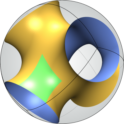
Figure 1. Free boundary minimal surface of genus 0 with tetrahedral symmetry and $4$ boundary components and its fundamental domain being a free boundary minimal disk inside a four-sided wedge.

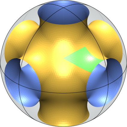
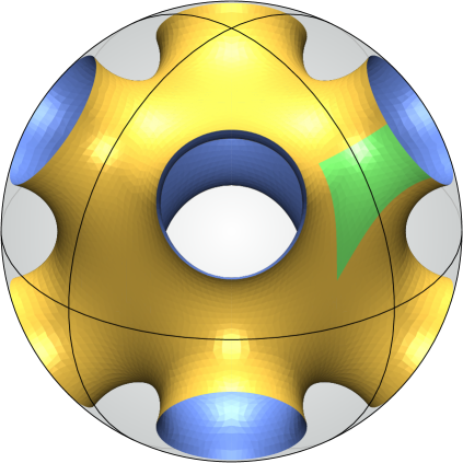
Figure 2. Free boundary minimal surfaces of genus $0$ with octahedral symmetry and $6$ or $8$ boundary components.

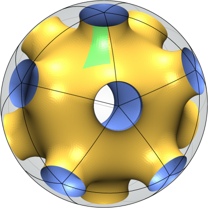
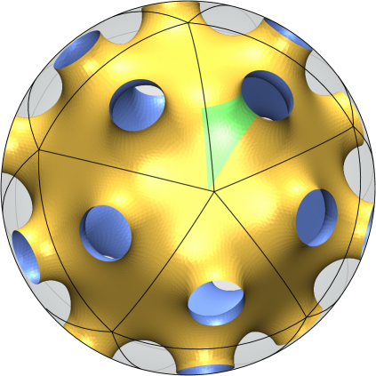
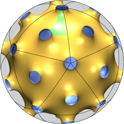
Figure 3. Free boundary minimal surfaces of genus $0$ with icosahedral symmetry and $12$, $20$ or $32$ boundary components.

Remark 1.15.

For Laplace eigenvalues, the eigenfunctions of a critical metric $g$ on $M$ for $\Lambda_{1}$ realise an isometric immersion of $M$ as a minimal surface in the sphere $\mathbb{S}^{m}$ for some $m$, see Nadirashvili [59].

Plan of the paper

In Section 2, we describe precisely the homogenisation construction in the Riemannian setting. Theorem 2.1 is a restatement of Theorem 1.1 in terms of the explicit sequence of domains for which the normalised Steklov eigenvalues converge to the weighted Laplace eigenvalues.

In Section 3 we prove various technical inequalities that will be used in the later stages. Some of these inequalities are known for domains in flat space and we extend their proofs to the Riemannian setting. We first need to control the norm of the traces $\gamma^{\varepsilon}:\mathrm{H}^{1}(\Omega^{\varepsilon})\to\mathrm{L}^{2}(\partial\Omega^{\varepsilon})$ and $\tau^{\varepsilon}:\mathrm{B}\mathrm{V}(\Omega^{\varepsilon})\to\mathrm{L}^{1}(\partial\Omega^{\varepsilon})$ uniformly in the parameter $\varepsilon$. We also need to bound uniformly the norm of the harmonic extension operator from $\mathrm{H}^{1}(\Omega^{\varepsilon})$ to $M$, and to have a uniform Poincaré–Wirtinger inequality for some topological perturbations of geodesically convex subsets of $M$. We point out that the usual sufficient conditions in term of conditions on tubular neighbourhoods of the boundary and inner cone conditions are not satisfied in our case, nevertheless we can use the structure of the problem to find the relevant bounds.

In Section 4, we prove boundedness properties for the Steklov eigenvalues and eigenfunctions of the domains $\Omega^{\varepsilon}$. More previsely, we prove that for every fixed $k$, $\sigma_{k}^{\varepsilon}$ is bounded in $\varepsilon$, and that the $\mathrm{L}^{\infty}$ norm of $u_{k}^{(\varepsilon)}$ is also bounded uniformly.

Section 5 is dedicated to the proof of Theorem 2.1. The proof proceeds in three main steps. The first one is to show that for every $k$, the eigenvalues $\sigma_{k}(\Omega^{\varepsilon})$ are bounded as $\varepsilon\to 0$ as well as to show that the families of harmonic extensions $U_{k}^{(\varepsilon)}$ are bounded in $\mathrm{H}^{1}(M)$. This gives us the existence along a subsequence of a limit $\sigma_{k}^{\varepsilon}\to\lambda$ and of a $\mathrm{H}^{1}(M)$ weak limit $U_{k}^{(\varepsilon)}\to\varphi$. The second step consists in studying the weak formulations to show that the pair $(\varphi,\lambda)$ is a solution to Problem (1). In the last step, we show that there is no mass lost in the process, and therefore that indeed $\lambda=\lambda_{k}(M,g,\beta)$.

In Section 6, we prove the isoperimetric inequality stated in Theorem 1.3 and give as a corollary explicit lower bounds on the maximiser for Steklov eigenvalues in terms of known bounds for Laplace eigenvalues.

Finally, in Section 7, we provide a proof of Theorem 1.13. This proof uses symmetries of the free boundary minimal surfaces, and properties of the nodal sets of first eigenfunctions.

Acknowledgements

We want to thank A. Fraser and R. Schoen for very useful discussions that led to better clarity in Appendix A. This project stemmed from a reading group at UCL, as such the authors want to thank in particular C. Belletini, F. Hiesmayr, M. Levitin, L. Parnovski, and F. Schulze for useful discussions and remarks as the project started, as well as I. Polterovich for raising the question leading to this paper. We would also like to thank H. Matthiesen and R. Petrides for very useful discussions about the state of the art concerning maximisers of normalised Steklov eigenvalues and free boundary minimal surfaces. We are grateful to M. Schulz for generously letting them use the pictures from his website [64]. Finaly, the authors would like to thank M. Karpukhin for very useful comments in the final stages of writing this paper.

AG acknowledges the support of NSERC. The research of JL was supported by EPSRC grant EP/P024793/1 and the NSERC Postdoctoral Fellowship.

2. The homogenisation construction

2.1. Notation

From this section on, we denote by $c$ and $C$ positive constants that may depend only on the manifold $(M,g)$, the dimension, and the positive smooth function $\beta\in C^{\infty}(M)$. Similarly, the homogenisation construction depends on a parameter $\varepsilon>0$ which must be chosen smaller than $\varepsilon_{0}>0$, a value also depending only on $(M,g)$, the dimension, and $\beta$. The precise values of $c,C$ and $\varepsilon_{0}$ may change from line to line, but changes occur only a finite number of times so that at the end $0<\varepsilon_{0},c,C<\infty$.

We will reserve the letters $\varphi,\lambda$ for general eigenfunctions and eigenvalues of Problem (1), and $\varphi_{k}$ and $\lambda_{k}$ representing specifically the $k$th ones. Similarly, we reserve $u^{(\varepsilon)}$ and $\sigma^{(\varepsilon)}$ for Steklov eigenvalues of the sequence of domains $\Omega^{\varepsilon}$. We drop in this notation any specific reference to $M$, to the metric $g$ and to the weight $\beta$ as they are kept fixed. We assume that eigenfunctions $u_{k}^{(\varepsilon)}$ and $\varphi_{k}$ are orthonormal, with respect to $\mathrm{L}^{2}(\partial\Omega^{\varepsilon})$ and $\mathrm{L}^{2}(M,\beta\,\mathrm{d}\mu_{g})$ respectively. We make use of various asymptotic notation.

• Indiscriminately, writing $f=O\left(g\right)$ or $f\ll g$ means that there exists $C,\varepsilon_{0}>0$ such that $\left\lvert f(x)\right\rvert\leq Cg(x)$ for all $0<x<\varepsilon_{0}$.

• Writing $f=o\left(g\right)$ means that $\frac{f}{g}\to 0$ as $\varepsilon\to 0$.

• Writing $f\asymp g$ means that both $f\ll g$ and $g\ll f$.

• Indices in the asymptotic notation (e.g. $f=O_{M}(g)$ or $f\ll_{k}g$) means that the implicit constants, the range of validity or the rate of convergence to $0$ for $o$ depends only on those quantities. We use $M$ as an index to represent dependence both on the manifold $M$ and on the metric $g$.

2.2. Geodesic polar coordinates

Some of our proofs are formulated using geodesic polar coordinates, so let us recall their construction, see [8, Chapter XII.8]. For a point $p\in M$ and $\delta<\operatorname{inj}(M)$, the exponential map is a diffeomorphism from the ball of radius $\delta$ in $T_{p}M$ to the geodesic ball $B_{\delta}(p)\subset M$. In $B_{\delta}(p)$, we use the polar coordinates $(\rho,\theta)$, where $\rho$ is the geodesic distance from $p$ and $\theta$ is a unit tangent vector in $T_{p}M$.

We recall that in those coordinates, the metric reads

$$g(\rho,\theta)=\,\mathrm{d}\rho^{2}+\rho^{2}(1+h(\rho,\theta))g_{\mathbb{S}^{d-1}},$$ (22)

where

$$\left\|h(\rho,\theta)\right\|_{\mathrm{C}^{1}(B_{\delta}(p))}=O_{M}(\delta).$$ (23)

We record as well that the volume element can be written in these coordinates as

$$\,\mathrm{d}V=\rho^{d-1}\left(1+O_{M}\left(\delta^{2}\right)\right)\,\mathrm{d}\rho\,\mathrm{d}A_{\mathbb{S}^{d-1}}$$ (24)

and for any geodesic sphere of radius $r\leq\delta$, its area element is of the form

$$\,\mathrm{d}A=r^{d-1}\left(1+O_{M}\left(r^{2}\right)\right)\,\mathrm{d}A_{\mathbb{S}^{d-1}}.$$ (25)

Compactness of $M$ ensures that the implicit constants in (23), (24) and (25) can be chosen independently of $p$.

2.3. Homogenisation by obstacles

For every $\varepsilon>0$, let $\mathbf{S}^{\varepsilon}$ be a maximal $\varepsilon$-separated subset of $M$, and let $\mathbf{V}^{\varepsilon}$ be the Voronoĭ tesselation associated with $\mathbf{S}^{\varepsilon}$, that is the set $\mathbf{V}^{\varepsilon}:=\left\{V_{p}^{\varepsilon}:p\in\mathbf{S}^{\varepsilon}\right\}$, with

$$V_{p}^{\varepsilon}:=\left\{x\in M:\operatorname{dist}(x,p)\leq\operatorname{dist}(x,q)\text{ for all }q\in\mathbf{S}^{\varepsilon}\right\}.$$ (26)

We note that for $\varepsilon<\varepsilon_{0}$ and every $p\in\mathbf{S}^{\varepsilon}$, $V_{p}^{\varepsilon}$ is a domain with piecewise smooth boundary, and that

$$\operatorname{Vol}_{g}(V_{p}^{\varepsilon})\asymp_{M}\varepsilon^{d}.$$ (27)

Indeed, by maximality of the $\varepsilon$-separated set $\mathbf{S}^{\varepsilon}$ we have that $B_{\varepsilon/2}(p)\subset V_{p}^{\varepsilon}\subset B_{3\varepsilon}(p)$. Let $\beta\in C^{\infty}(M)$ be a smooth positive function. For every $p\in\mathbf{S}^{\varepsilon}$, let $r_{\varepsilon,p}>0$ be such that

$$\mathcal{H}^{d-1}(\partial B_{r_{\varepsilon,p}}(p))=\beta(p)\operatorname{Vol}_{g}(V_{p}^{\varepsilon}).$$ (28)

It also follows from (24) and (25) that

$$r_{\varepsilon,p}\asymp_{M,\beta}\varepsilon^{\frac{d}{d-1}}.$$ (29)

Since the previous display holds uniformly for $p\in M$, we often abuse notation and write $r_{\varepsilon}$ for $r_{\varepsilon,p}$. We set

$$\mathbf{T}^{\varepsilon}:=\bigcup_{p\in\mathbf{S}^{\varepsilon}}B_{r_{\varepsilon}}(p),$$ (30)

$\Omega^{\varepsilon}=M\setminus\mathbf{T}^{\varepsilon}$, and $Q_{p}^{\varepsilon}=V_{p}^{\varepsilon}\setminus B_{r_{\varepsilon}}(p)$. See Figure 4 for a depiction of this construction.

Figure 4. Voronoĭ tesselation associated with a maximal $\varepsilon$-separated subset

Furthermore, we have that $\operatorname{dist}(B_{r_{\varepsilon,p}}(p),B_{r_{\varepsilon,q}}(q))\geq\varepsilon-O_{M,\beta}\left(\varepsilon^{\frac{d}{d-1}}\right)$ for all $p\neq q\in\mathbf{S}^{\varepsilon}$. We see that by construction, for every $0<\varepsilon<\varepsilon_{0}$,

$$\mathcal{H}^{d-1}(\partial\Omega^{\varepsilon})=\sum_{p\in\mathbf{S}^{\varepsilon}}\beta(p)\operatorname{Vol}_{g}(V_{p}^{\varepsilon}).$$ (31)

It also easy to see that the measure $\,\mathrm{d}A_{g}$ obtained on $M$ by restriction of the Hausdorff measure $\mathcal{H}^{d-1}$ to $\partial\Omega^{\varepsilon}$ converges weak-$*$ to the weighted Lebesgue measure $\beta\,\mathrm{d}\mu_{g}$ on $M$. That is, for each continuous function $f$ on $M$,

$$\int_{\partial\Omega^{\varepsilon}}f\,\mathrm{d}A_{g}\xrightarrow{\varepsilon\to 0}\int_{M}f\,\beta\,\mathrm{d}\mu_{g}.$$ (32)

This already addresses the first part of Theorem 1.1, and by considering $f\equiv 1$ in (32) we see that

$$\mathcal{H}^{d-1}(\partial\Omega^{\varepsilon})\xrightarrow{\varepsilon\to 0}\int_{M}\beta\,\mathrm{d}\mu_{g}.$$ (33)

We study the sequence of eigenvalue problems on $\Omega^{\varepsilon}$

$$\begin{cases}\Delta u^{(\varepsilon)}=0&\text{in }\Omega^{\varepsilon};\\ \partial_{\nu}u^{(\varepsilon)}=\sigma^{(\varepsilon)}u^{(\varepsilon)}&\text{on }\partial\Omega^{\varepsilon},\end{cases}$$ (34)

and for every eigenfunction $u_{k}^{(\varepsilon)}$, we define $U_{k}^{(\varepsilon)}:M\to\mathbb{R}$ as the unique function equal to $u_{k}^{(\varepsilon)}$ on $\overline{\Omega^{\varepsilon}}$ and harmonic in $\mathbf{T}^{\varepsilon}$. The next theorem is the central technical result of this paper, and is in the flavour of the main theorem of [34]. It is also readily seen to imply directly Theorem 1.1 by providing the appropriate sequence $\Omega^{\varepsilon}$.

Theorem 2.1.

The eigenvalues $\sigma_{k}^{(\varepsilon)}$ of Problem (34) converge as $\varepsilon\to 0$ to the eigenvalue $\lambda_{k}(M,g,\beta)$ defined in Problem (1). Up to choosing a subsequence, the extensions $U_{k}^{(\varepsilon)}$ to $M$ of the eigenfunctions $u_{k}^{(\varepsilon)}$ converge weakly in $\mathrm{H}^{1}(M)$ to the corresponding Laplace eigenfunction $f_{k}$ on $M$, where $f_{k}$ is normalised to $\mathrm{L}^{2}(M,\beta\,\mathrm{d}\mu_{g})$ norm $1$.

The proof is split in two main steps and is the subject of Section 5.

The first step is to show that there is a subsequence $(\sigma_{k}^{(\varepsilon)},U_{k}^{(\varepsilon)})$ converging to a weak solution $(\lambda,\varphi)$ of the weighted Laplace eigenvalue problem. In other words, the pair $(\lambda,\varphi)$ satisfies

$$\forall v\in\mathrm{H}^{1}(M),\qquad\int_{M}\nabla v\cdot\nabla\varphi\,\mathrm{d}\mu_{g}=\lambda\int_{M}v\,\varphi\,\beta\,\mathrm{d}\mu_{g}.$$ (35)

The second step consists in proving that $(\lambda,\varphi)$ has to be the $k$th eigenpair of the weighted Laplace eigenvalue problem. This will be done by showing that in the limit the functions $U_{k}^{(\varepsilon)}$ do not lose any mass. Physically, this can be interpreted as an instance of the Fermi exclusion principle, see. e.g. the work of Colin de Verdière [21] for an early application of such an idea to create manifolds whose first Laplace eigenvalue have large multiplicity.

3. Analytic properties of perforated domains

In this section we describe analytic properties of the perforated manifolds $\Omega^{\varepsilon}$ and of the Voronoĭ cells $V_{p}^{\varepsilon}$. More precisely, we show that trace and extension operators are well behaved in the homogenisation limiting process. We stress that many of the inequalities we show here would be obviously satisfied for a fixed domain $\Omega$. However, the usual sufficient conditions under which those inequalities would hold uniformly for a family of domains $\Omega^{\varepsilon}$ either are not satisfied, or it is nontrivial to show that they are indeed satisfied. We start by proving three lemmata about norms of trace operators. We denote the annuli $A_{p}^{\varepsilon}:=B_{\varepsilon/2}(p)\setminus B_{r_{\varepsilon}}(p)$.

The statement of Lemma 3.1 below is a generalisation of [6, Proposition 5.1] for domains in a closed manifold. For domains $\Omega\subset M$ whose boundary is not necessarily piecewise smooth, we denote by $\operatorname{Per}(\Omega,M)$ their perimeter in $M$, which corresponds to the Hausdorff measure of their reduced boundary $\partial^{*}\Omega$. Note that the topological boundary may in general be larger than the reduced boundary.

Lemma 3.1.

Let $\left\{\Omega_{n}\subset M:n\in\mathbb{N}\right\}$ be a sequence of open, bounded domains such that $\mathcal{H}^{d-1}(\partial\Omega_{n})$ is uniformly bounded. Assume that there exists $Q,\delta>0$ such that for all $n\in\mathbb{N}$ and $x\in\partial\Omega_{n}$,

$$\sup\left\{\frac{\mathcal{H}^{d-1}(\partial^{*}E\cap\partial^{*}\Omega_{n})}{\mathcal{H}^{d-1}(\partial^{*}E\cap\Omega_{n})}:E\subset\Omega_{n}\cap B_{\delta}(x),\operatorname{Per}(E,\Omega_{n})<\infty\right\}<Q.$$ (36)

Then, the trace operators $\tau_{n}:\mathrm{B}\mathrm{V}(\Omega_{n})\to\mathrm{L}^{1}(\partial\Omega_{n})$ are bounded uniformly in $n$.

Proof.

For any $\eta>0$, since $M$ is compact, we can choose $\delta$ small enough so that for every $x\in M$, the metric in geodesic polar coordinates in $B_{2\delta}(x)$ reads

$$g=\,\mathrm{d}\rho^{2}+\rho^{2}(1+h(\rho,\theta))\,\mathrm{d}\theta^{2},$$ (37)

with $\left\lvert h(\rho,\theta)\right\rvert+\left\lvert\nabla h(\rho,\theta)\right\rvert\leq\delta^{1/2}\leq\eta$. In other word, the diffeomorphism provided by the inverse of the exponential map, from $B_{2\delta}(x)$ to the ball of radius $2\delta$ in $\mathbb{R}^{d}$ is a $\mathrm{C}^{1}$ $\eta$-perturbation of an isometry. For any $n$, the norms of $\mathrm{L}^{1}(\partial\Omega_{n}\cap B_{\delta}(x))$ and $\mathrm{B}\mathrm{V}(\Omega_{n}\cap B_{\delta}(x))$ change uniformly continuously on bounded sets under $\mathrm{C}^{1}$ diffeomorphisms, and the same is true of the Hausdorff measures in (36). By [6, Proposition 5.1], (36) implies that the trace operators are uniformly bounded on the pullbacks to the balls, and by the above discussion we can bring these estimates back to the manifold. ∎

Lemma 3.2.

The trace operators $\tau^{\varepsilon}:\mathrm{B}\mathrm{V}(\Omega^{\varepsilon})\to\mathrm{L}^{1}(\partial\Omega^{\varepsilon})$ are bounded uniformly in $\varepsilon$.

Proof.

In order to apply Lemma 3.1, we need to find $\delta,Q>0$ such that for all $x\in\partial\Omega^{\varepsilon}$ and all $\varepsilon>0$, (36) holds. A simple volume comparison yields that there is $c>0$ such that for all $\delta>0$ and $x\in\partial\Omega^{\varepsilon}$,

$$\#\left\{p\in\mathbf{S}^{\varepsilon}:Q_{p}^{\varepsilon}\cap B_{\delta}(x)\neq\varnothing\right\}\leq c\left(\frac{\delta}{\varepsilon}\right)^{d}.$$ (38)

Combining (38) with (28), for any $E\subset\Omega^{\varepsilon}\cap B_{\delta}(x)$ of finite perimeter,

$$\mathcal{H}^{d-1}(\partial^{*}E\cap\partial\Omega^{\varepsilon})\leq\mathcal{H}^{d-1}(\partial\Omega^{\varepsilon}\cap B_{\delta}(x))\leq C\delta^{d},$$ (39)

where $C$ depends on $M$, $g$ and $\beta$. We may then assume that the supremum is taken over sets $E$ such that

$$\mathcal{H}^{d-1}(\partial^{*}E\cap\Omega^{\varepsilon})\leq C\delta^{d},$$ (40)

otherwise the ratio in (36) is bounded by $1$. Observe that

$$\mathcal{H}^{d-1}(\partial^{*}E\cap\partial\Omega^{\varepsilon})=\sum_{p\in\mathbf{S}^{\varepsilon}}\mathcal{H}^{d-1}(\partial^{*}E\cap\partial B_{r_{\varepsilon}}(p)).$$ (41)

For $p\in\mathbf{S}^{\varepsilon}$ and $t\in(0,\varepsilon/4)$, define

$$F_{p,t}=E\cap\left\{x:\operatorname{dist}(x,\partial B_{r_{\varepsilon}}(p))\leq t\right\}.$$ (42)

Assume that for some $t\in(0,\varepsilon/4)$ we have that

$$\mathcal{H}^{d-1}(\partial^{*}F_{p,t}\cap Q_{p}^{\varepsilon})\leq 2\mathcal{H}^{d-1}(\partial^{*}E\cap Q_{p}^{\varepsilon}).$$ (43)

Without loss of generality, we have chosen $\delta$ small enough so that the retraction on a geodesic ball of radius $\delta^{\prime}<\delta$ is a $2$-Lipschitz map uniformly for $x\in M$. This means that

$$\mathcal{H}^{d-1}(\partial^{*}E\cap\partial B_{r_{\varepsilon}}(p)) =\mathcal{H}^{d-1}(\partial^{*}F_{p,t}\cap\partial B_{r_{\varepsilon}}(p))$$ (44)

$$\leq 2\mathcal{H}^{d-1}(\partial^{*}F_{p,t}\cap Q_{p}^{\varepsilon})$$

$$\leq 4\mathcal{H}^{d-1}(\partial^{*}E\cap Q_{p}^{\varepsilon}).$$

Let $\widetilde{\mathbf{S}}^{\varepsilon}=\left\{p\in\mathbf{S}^{\varepsilon}:\eqref{eq:localised}\text{ does not hold}\right\}$. If $\widetilde{\mathbf{S}}^{\varepsilon}$ is empty, our claim holds since in that case (44) implies that (36) holds with $Q=4$. Let $p\in\widetilde{\mathbf{S}}^{\varepsilon}$.

Setting

$$h_{p}(t):=\mathcal{H}^{d-1}\left(\partial^{*}F_{p,t}\cap\left\{x:\operatorname{dist}(x,\partial B_{r_{\varepsilon}}(p))=t\right\}\right),$$ (45)

the coarea formula gives $\partial_{t}\operatorname{Vol}_{g}(F_{p,t})=h_{p}(t)$. It follows from the relative isoperimetric inequality [26, Theorem 5.6.2] that there is a constant $c>0$ depending on $M$ such that

$$c\operatorname{Vol}_{g}(F_{p,t})^{\frac{d-1}{d}} \leq\mathcal{H}^{d-1}(\partial^{*}F_{p,t}\cap Q_{p}^{\varepsilon})$$ (46)

$$\leq 2h_{p}(t),$$

where the second inequality follows from (43) not holding at $p$. Integrating, we therefore have that

$$2\operatorname{Vol}_{g}(F_{p,\varepsilon/4}) =\left(\int_{0}^{\varepsilon/4}\frac{h_{p}(t)}{\operatorname{Vol}_{g}(F_{p,t})^{\frac{d-1}{d}}}\,\mathrm{d}t\right)^{d}$$ (47)

$$\gg_{M}C\varepsilon^{d}$$

$$\gg_{M,\beta}C\mathcal{H}^{d-1}(\partial B_{r_{\varepsilon}}(p)).$$

On the other hand, it follows from the isoperimetric inequality and equation (44) that

$$\sum_{p\in\widetilde{\mathbf{S}}^{\varepsilon}}\operatorname{Vol}_{g}(E\cap Q_{p}^{\varepsilon}) \ll_{M,\beta}\mathcal{H}^{d-1}(\partial^{*}E)^{\frac{d}{d-1}}$$ (48)

$$\ll_{M,\beta}\left(\mathcal{H}^{d-1}(\partial^{*}E\cap\Omega^{\varepsilon})+\mathcal{H}^{d-1}(\partial^{*}E\cap\partial\Omega^{\varepsilon})\right)^{\frac{d}{d-1}}$$

$$\ll_{M,\beta}\Biggl{(}\mathcal{H}^{d-1}(\partial^{*}E\cap\Omega^{\varepsilon})+\sum_{p\in\widetilde{\mathbf{S}}^{\varepsilon}}\mathcal{H}^{d-1}(B_{r_{\varepsilon}}(p))\Biggr{)}^{\frac{d}{d-1}}.$$

Summing over $p\in\widetilde{\mathbf{S}}^{\varepsilon}$ in (47) and inserting in (48), we obtain $C$ depending only on $M$ and $\beta$ such that

$$1\leq C\Biggl{(}\sum_{p\in\widetilde{\mathbf{S}}^{\varepsilon}}\mathcal{H}^{d-1}(B_{r_{\varepsilon}}(p))\Biggr{)}^{\frac{1}{d-1}}\left(1+\frac{\mathcal{H}^{d-1}(\partial^{*}E\cap\Omega^{\varepsilon})}{\sum_{p\in\widetilde{\mathbf{S}}^{\varepsilon}}\mathcal{H}^{d-1}(\partial B_{r_{\varepsilon}}(p))}\right)^{\frac{d}{d-1}}.$$ (49)

It follows from the weak-$*$ convergence in (32) that for small enough $\varepsilon$,

$$\mathcal{H}^{d-1}(\partial\Omega^{\varepsilon}\cap B_{\delta}(x))<2\max_{p}\beta(p)\operatorname{Vol}_{g}(B_{\delta}(x)).$$ (50)

This means that we can choose $\delta$ small enough, depending on $M$ and $\beta$ but not on $\varepsilon$ so that

$$C\Biggl{(}\sum_{p\in\widetilde{\mathbf{S}}^{\varepsilon}}\mathcal{H}^{d-1}(\partial B_{r_{\varepsilon}}(p))\Biggr{)}^{\frac{d}{d-1}}\leq\frac{1}{4},$$ (51)

which means that

$$1\leq\frac{\mathcal{H}^{d-1}(\partial^{*}E\cap\Omega^{\varepsilon})}{\sum_{p\in\widetilde{\mathbf{S}}^{\varepsilon}}\mathcal{H}^{d-1}(\partial B_{r_{\varepsilon}}(p))}.$$ (52)

Combining estimates (44) with (52) gives us that for $\varepsilon$ small enough,

$$\mathcal{H}^{d-1}(\partial^{*}E\cap\partial\Omega^{\varepsilon})\leq 4\mathcal{H}^{d-1}(\partial^{*}E\cap\Omega^{\varepsilon}),$$ (53)

establishing our claim. ∎

The following lemma follows from the previous one rather directly, but we state it explicitly for ease of reference.

Lemma 3.3.

The Sobolev trace operators $\gamma^{\varepsilon}:\mathrm{H}^{1}(\Omega^{\varepsilon})\to\mathrm{L}^{2}(\partial\Omega^{\varepsilon})$ are bounded uniformly in $\varepsilon$.

Proof.

Observe first that if $f\in\mathrm{H}^{1}(\Omega^{\varepsilon})$, then $f^{2}\in\mathrm{B}\mathrm{V}(\Omega^{\varepsilon})$. Indeed, $\left\|f\right\|_{\mathrm{L}^{2}(\Omega^{\varepsilon})}^{2}=\left\|f^{2}\right\|_{\mathrm{L}^{1}(\Omega^{\varepsilon})}$, and

$$\int_{\Omega^{\varepsilon}}\left\lvert\nabla f^{2}\right\rvert\,\mathrm{d}\mu_{g} =\int_{\Omega^{\varepsilon}}2\left\lvert f\nabla f\right\rvert\,\mathrm{d}\mu_{g}$$ (54)

$$\leq\int_{\Omega^{\varepsilon}}f^{2}+\left\lvert\nabla f\right\rvert^{2}\,\mathrm{d}\mu_{g}.$$

We therefore have

$$\left\|f\right\|_{\mathrm{L}^{2}(\partial\Omega^{\varepsilon})}^{2} =\left\|f^{2}\right\|_{\mathrm{L}^{1}(\partial\Omega^{\varepsilon})}$$ (55)

$$\leq C\left\|f^{2}\right\|_{\mathrm{B}\mathrm{V}(\Omega^{\varepsilon})}$$

$$\leq 2C\left\|f\right\|_{\mathrm{H}^{1}(\Omega^{\varepsilon})}^{2},$$

proving our claim. ∎

The next Lemma describes the behaviour of the operator of harmonic extension inside the holes $\mathbf{T}^{\varepsilon}$.

Lemma 3.4.

The harmonic extension operator $h^{\varepsilon}:\mathrm{H}^{1}(\Omega^{\varepsilon})\to\mathrm{H}^{1}(\mathbf{T}^{\varepsilon})$ has norm uniformly bounded in $\varepsilon$. Furthermore,

$$\left\|h^{\varepsilon}\right\|_{\mathrm{H}^{1}(\Omega^{\varepsilon})\to\mathrm{L}^{2}(\mathbf{T}^{\varepsilon})}\xrightarrow{\varepsilon\to 0}0.$$ (56)

Proof.

It is clearly sufficient to show that for $\delta$ small enough and $p\in\Omega$, the harmonic extension operator $\mathrm{H}^{1}(B_{2\delta}(p)\setminus B_{\delta}(p))\to\mathrm{H}^{1}(B_{\delta}(p))$ is bounded uniformly in $\delta$, and that the $\mathrm{L}^{2}$ norm of the harmonic extension in $B_{\delta}(p)$ goes to $0$. This follows directly from [63, Example 1, p. 40], where this is shown in the Euclidean setting and the observation that for small enough $\delta$, c.f. equation (24), geodesic balls and spherical shells are mapped to Euclidean balls and spherical shells by $\mathrm{C}^{1}$-small perturbations of an isometry, and that all quantities involved are uniformly continuous in such perturbations. ∎

Finally, we will require that the Poincaré–Wirtinger inequality of the perforated Voronoĭ cells $Q_{p}^{\varepsilon}$ hold uniformly in both $p\in M$ and $\varepsilon>0$. To this end, for any domain $\Omega\subset M$, denote by $\mu_{1}(\Omega)$ the first non-trivial Neumann eigenvalue of $\Omega$, and for any $f:U\subset M\to\mathbb{R}$,

$$m_{f}:=\int_{U}f\,\mathrm{d}\mu_{g}.$$ (57)

Lemma 3.5.

There is $c,\varepsilon_{0}>0$ depending only on $M$ and $\beta$ such that for $0<\varepsilon<\varepsilon_{0}$, $p\in\mathbf{S}^{\varepsilon}$, and all $f\in\mathrm{H}^{1}(Q_{p}^{\varepsilon})$

$$\int_{Q_{p}^{\varepsilon}}\left\lvert f-m_{f}\right\rvert^{2}\,\mathrm{d}\mu_{g}\leq c\varepsilon^{2}\int_{Q_{p}^{\varepsilon}}\left\lvert\nabla f\right\rvert^{2}\,\mathrm{d}\mu_{g}.$$ (58)

Proof.

It follows from the variational characterisation for Neumann eigenvalues that

$$\int_{Q_{p}^{\varepsilon}}\left\lvert f-m_{f}\right\rvert^{2}\,\mathrm{d}\mu_{g}\leq\frac{1}{\mu_{1}(Q_{p}^{\varepsilon})}\int_{Q_{p}^{\varepsilon}}\left\lvert\nabla f\right\rvert^{2}\,\mathrm{d}\mu_{g}$$ (59)

so that it is equivalent to show that for all $0<\varepsilon<\varepsilon_{0}$,

$$\mu_{1}(Q_{p}^{\varepsilon})\geq c^{-1}\varepsilon^{-2}$$ (60)

for some $c>0$.

Since the Voronoĭ cells $V_{p}^{\varepsilon}$ are geodesically convex and have diameter $\operatorname{diam}(V_{p}^{\varepsilon})=O\left(\varepsilon\right)$, uniformly in $p\in\mathbf{S}^{\varepsilon}$, it follows from [37, Theorem 1.2] that there is a constant $C$ depending only on the curvature and dimension of $M$ such that

$$\mu_{1}(V_{p}^{\varepsilon})\geq C\varepsilon^{-2}.$$ (61)

Let $w$ be the first non-constant Neumann eigenfunction of $Q_{p}^{\varepsilon}$, normalised to $\left\|w\right\|_{\mathrm{L}^{2}(Q_{p}^{\varepsilon})}=1$, and let $\widehat{w}$ be the function defined on $V_{p}^{\varepsilon}$ as the harmonic extension to $B_{r_{\varepsilon}}(p)$, i.e. as

$$\widehat{w}(x)=\begin{cases}w(x)&\text{if }x\in Q_{p}^{\varepsilon}\\ h^{\varepsilon}w(x)&\text{if }x\in B_{r_{\varepsilon}}(p),\end{cases}$$ (62)

where $h^{\varepsilon}$ is defined in Lemma 3.4. It follows from the Cauchy–Schwarz inequality and Lemma 3.4 that

$$m_{w}:=\int_{V_{p}^{\varepsilon}}\widehat{w}(x)\,\mathrm{d}\mu_{g}=\int_{B_{r_{\varepsilon}}(p)}h^{\varepsilon}w(x)\,\mathrm{d}A_{g}=o\left(\varepsilon^{\frac{d^{2}}{2(d-1)}}\right).$$ (63)

Using $\widehat{w}-m_{w}$ as a test function for the first Neumann eigenvalue in $V_{p}^{\varepsilon}$ we have from Lemma 3.4 that there is a constant $c$ such that

$$\mu_{1}(Q_{p}^{\varepsilon}) =\int_{Q_{p}^{\varepsilon}}\left\lvert\nabla(\widehat{w}-m_{w})\right\rvert^{2}\,\mathrm{d}\mu_{g}$$ (64)

$$\geq c\int_{V_{p}^{\varepsilon}}\left\lvert\nabla(\widehat{w}-m_{w})\right\rvert^{2}\,\mathrm{d}\mu_{g}$$

$$\geq c\mu_{1}(V_{p}^{\varepsilon})\left\|\widehat{w}-m_{w}\right\|^{2}_{\mathrm{L}^{2}(V_{p}^{\varepsilon})}$$

$$\geq c\varepsilon^{-2}(1+o\left(1\right)),$$

concluding the proof. ∎

4. Analytic properties of Steklov eigenpairs

In this section, we obtain analytic properties of the Steklov eigenvalues $\sigma_{k}^{(\varepsilon)}:=\sigma_{k}(\Omega^{\varepsilon})$, and of Steklov eigenfunctions $u_{k}^{(\varepsilon)}$. We start by obtaining bounds on $\sigma_{k}^{(\varepsilon)}$ which are uniform in $\varepsilon$.

Lemma 4.1.

For all $k\in\mathbb{N}$, $\beta\in C^{\infty}(M)$, we have as $\varepsilon\to 0$

$$\sigma_{k}^{(\varepsilon)}:=\sigma_{k}(\Omega^{\varepsilon})\leq\lambda_{k}(M,g,\beta)+o_{M,k,\beta}(1).$$ (65)

Proof.

It is clearly sufficient to prove this statement for $\varepsilon<\varepsilon_{0}$ small enough. It follows from the variational characterisation of Steklov eigenvalues that

$$\sigma_{k}^{(\varepsilon)}=\min_{\begin{subarray}{c}E\subset\mathrm{L}^{2}(\partial\Omega^{\varepsilon})\\ \dim(E)=k+1\end{subarray}}\max_{u\in E}\frac{\int_{\Omega^{\varepsilon}}\left\lvert\nabla u\right\rvert^{2}\,\mathrm{d}\mu_{g}}{\int_{\partial\Omega^{\varepsilon}}u^{2}\,\mathrm{d}x}.$$ (66)

Let $f_{0},\dotsc,f_{k}$ be the first $k+1$ normalised eigenfunctions of the weighted Laplacian on $M$. They are pairwise $\mathrm{L}^{2}(M,\beta\,\mathrm{d}\mu_{g})$ orthogonal, and since the $(d-1)$-dimensional Hausdorff measure restricted to $\partial\Omega^{\varepsilon}$ converges weak-$*$ to $\beta\,\mathrm{d}\mu_{g}$, for $\varepsilon$ small enough they span a $k+1$ dimensional subspace of $\mathrm{L}^{2}(\partial\Omega^{\varepsilon})$, and for $0\leq j\leq k$,

$$\left\|f_{j}\right\|_{\mathrm{L}^{2}(\partial\Omega^{\varepsilon})}^{2} =\int_{M}f_{j}^{2}(x)\beta(x)\,\mathrm{d}\mu_{g}+o_{M,k,\beta}(1).$$ (67)

Therefore, using $E=\operatorname{span}(f_{0},\dotsc,f_{k})$ as a test subspace for $\sigma_{k}^{\varepsilon}$ yields

$$\sigma_{k}^{(\varepsilon)} \leq\max_{f\in E}\frac{\int_{\Omega^{\varepsilon}}\left\lvert\nabla f\right\rvert^{2}\,\mathrm{d}\mu_{g}}{\int_{\partial\Omega^{\varepsilon}}f^{2}\,\mathrm{d}\mu_{g}}$$ (68)

$$\leq\lambda_{k}(M,g,\beta)+o_{M,k,\beta}(1),$$

which is what we set out to prove. ∎

We turn to the boundedness of the sequence $\left\{u_{k}^{(\varepsilon)}\right\}$ in $\mathrm{L}^{\infty}(\Omega^{\varepsilon})$.

Lemma 4.2.

There is a $\varepsilon_{0},C>0$ depending only on $k,\beta,M$ such that for all $0<\varepsilon<\varepsilon_{0}$,

$$\left\|u_{k}^{(\varepsilon)}\right\|_{\mathrm{L}^{\infty}(\Omega^{\varepsilon})}\leq C$$ (69)

Proof.

It is shown in [6, Theorem 3.1] that for any Steklov eigenfunction $u$ with eigenvalue $\sigma$ on a domain $\Omega$,

$$\left\|u\right\|_{\mathrm{L}^{\infty}(\Omega)}\leq C\left\|u\right\|_{\mathrm{L}^{2}(\partial\Omega)},$$ (70)

with $C$ depending polynomially only on $\sigma$, $\operatorname{Vol}_{g}(\Omega)$ and the norm of the trace operator $\tau:\mathrm{B}\mathrm{V}(\Omega)\to\mathrm{L}^{1}(\partial\Omega)$. Note that they only prove this statement for domains in $\mathbb{R}^{d}$, however a close inspection of their proof reveals that geometric dependence appears in only two places. The first one is on the norm of the extension operator from $\mathrm{B}\mathrm{V}(\Omega)\to\mathrm{B}\mathrm{V}(M)$, which depends only on the norm of $\tau$ (see [26][Theorem 5.4.1]), and therefore is already accounted for. The second one is on the norm of the Sobolev embedding $\mathrm{B}\mathrm{V}(M)\to\mathrm{L}^{\frac{d}{d-1}}(M)$, whose norm depends only on the Gagliardo–Nirenberg–Sobolev inequality, which chnages by at most a constant for $M$ compact.

Lemma 3.2 gives a uniform bound for $\left\|\tau^{\varepsilon}\right\|$, Lemma 4.1 gives us a uniform bound for $\sigma_{k}^{(\varepsilon)}$ while $\operatorname{Vol}_{g}(\Omega)$ is obviously bounded by $\operatorname{Vol}_{g}(M)$ and $u_{k}^{(\varepsilon)}$ is normalised to $\|u_{k}^{(\varepsilon)}\|_{\mathrm{L}^{2}(\partial\Omega^{\varepsilon})}=1$. Thus $\|u_{k}^{(\varepsilon)}\|_{\mathrm{L}^{\infty}}$ is bounded, uniformly in $\varepsilon$. ∎

5. The homogenisation limit

In this section, we prove Theorem 2.1. While the general scheme of the proof follows the general idea in [34], we cannot use any periodic structure in order to define the auxiliary functions required to prove convergence. The major difference with general homogenisation methods will be the definition of those auxiliary functions on a cell by cell basis in such a way as to obtain the desired convergence.

Our first step is to show that there are converging subsequences. This is done in the following lemma. Recall that $u_{k}^{(\varepsilon)}$ are the Steklov eigenfunctions on $\Omega^{\varepsilon}$ and $U_{k}^{(\varepsilon)}$ their extension to $M$, harmonic in $\mathbf{T}^{\varepsilon}$.

Lemma 5.1.

There is a subsequence of $\left\{U_{k}^{(\varepsilon)}\right\}$, which we still label by $\varepsilon$, converging weakly in $\mathrm{H}^{1}(M)$.

Proof.

It suffices to show that the sequence $\left\{U_{k}^{(\varepsilon)}\right\}$ is bounded in $\mathrm{H}^{1}(\Omega)$ as $\varepsilon\to 0$. By Lemma 3.4, we have that

$$\left\|U_{k}^{(\varepsilon)}\right\|_{\mathrm{H}^{1}(M)}\ll_{M,\beta}\left\|u_{k}^{(\varepsilon)}\right\|_{\mathrm{H}^{1}(\Omega^{\varepsilon})}$$ (71)

On the other hand, we have that

$$\left\|\nabla u_{k}^{(\varepsilon)}\right\|_{\mathrm{L}^{2}(\Omega^{\varepsilon})^{d}}^{2}\leq\sigma_{k}^{(\varepsilon)}\leq\lambda_{k}(M,g,\beta)+o_{M,\beta,k}\left(1\right),$$ (72)

where the last bound follows from Lemma 4.1. Furthermore, it follows from Lemma 4.2 that

$$\left\|u_{k}^{(\varepsilon)}\right\|_{\mathrm{L}^{2}(\Omega^{\varepsilon})}\leq\operatorname{Vol}_{g}(\Omega^{\varepsilon})^{1/2}\left\|u_{k}^{(\varepsilon)}\right\|_{\mathrm{L}^{\infty}(\Omega^{\varepsilon})}=O_{M,\beta}\left(1\right).$$

Combining all of this yields indeed that the sequence $\left\{U_{k}^{(\varepsilon)}\right\}$ is uniformly bounded in $\mathrm{H}^{1}(M)$, so that it has a subsequence weakly converging in $\mathrm{H}^{1}(M)$. ∎

Proposition 5.2.

Let $k\in\mathbb{N}$. As $\varepsilon\to 0$, the pairs $(U_{k}^{(\varepsilon)},\sigma_{k}^{(\varepsilon)})$ converge to a pair $(f,\lambda)$, so that $f$ is an eigenfunction of the weighted Laplace problem on $M$ with eigenvalue $\lambda$, the convergence of $U_{k}^{(\varepsilon)}$ being weak in $\mathrm{H}^{1}$.

Proof.

Denote by $(\varphi,\lambda)$ the weak limit (up to a subsequence) of $(U_{k}^{(\varepsilon)},\sigma_{k}^{(\varepsilon)})$, we now aim to show that they are weak solutions of the weighted Laplace eigenvalue problem on $M$, i.e. that they satisfy (35). For a real valued $v\in\mathrm{H}^{1}(M)$, we have, using the weak formulation of Problem (34) that

$$\int_{M}\nabla U_{k}^{(\varepsilon)}\cdot\nabla v\,\mathrm{d}\mu_{g}=\sigma_{k}^{(\varepsilon)}\int_{\partial\Omega^{\varepsilon}}U_{k}^{(\varepsilon)}v\,\mathrm{d}A_{g}+\int_{\mathbf{T}^{\varepsilon}}\nabla U_{k}^{(\varepsilon)}\cdot\nabla v\,\mathrm{d}\mu_{g}.$$ (73)

In order to be able to consider smooth test functions in this weak formulation, we need to ensure that the family of bounded linear functionals $\Phi^{\varepsilon}\in\mathrm{H}^{1}(M)^{*}$ given by

$$\Phi^{\varepsilon}(v):=\sigma_{k}^{(\varepsilon)}\int_{\partial\Omega^{\varepsilon}}U_{k}^{(\varepsilon)}v\,\mathrm{d}A_{g}.$$ (74)

is bounded uniformly in $\varepsilon<\varepsilon_{0}$. It indeed is, since we know from Lemma 4.1 that $\sigma_{k}^{(\varepsilon)}$ is bounded as $\varepsilon\to 0$, and we have

$$\left\lvert\int_{\partial\Omega^{\varepsilon}}U_{k}^{(\varepsilon)}v\,\mathrm{d}A_{g}\right\rvert \leq\left\|\gamma^{\varepsilon}\right\|_{\mathrm{H}^{1}(\Omega^{\varepsilon})\to\mathrm{L}^{2}(\partial\Omega^{\varepsilon})}^{2}\left\|U_{k}^{(\varepsilon)}\right\|_{\mathrm{L}^{2}(\partial\Omega^{\varepsilon})}\left\|v\right\|_{\mathrm{H}^{1}(M)}$$ (75)

$$=\left\|\gamma^{\varepsilon}\right\|_{\mathrm{H}^{1}(\Omega^{\varepsilon})\to\mathrm{L}^{2}(\partial\Omega^{\varepsilon})}^{2}\left\|v\right\|_{\mathrm{H}^{1}(M)}.$$

We have shown in Lemma 3.3 that $\left\|\gamma^{\varepsilon}\right\|$ was bounded uniformly in $\varepsilon$ for $0<\varepsilon<\varepsilon_{0}$. By the Banach-Steinhaus theorem, the family $\left\{\Phi^{\varepsilon}\right\}$ is uniformly bounded. We may assume from now on that in the weak formulation of Problem (34), we consider only $v$ in a dense subspace of $\mathrm{H}^{1}(M)$, in particular we assume $v\in\mathrm{C}^{\infty}(M)$.

That the first term in (73) converges follows from weak convergence of $U_{k}^{(\varepsilon)}$. That the last term in (73) converges to $0$ follows from the Cauchy–Schwarz inequality and the observation that since $v\in\mathrm{C}^{\infty}(M)$,

$$\int_{\mathbf{T}^{\varepsilon}}\left\lvert\nabla v\right\rvert^{2}\,\mathrm{d}\mu_{g}\leq\max_{x\in M}\left\lvert\nabla v(x)\right\rvert^{2}\operatorname{Vol}_{g}(\mathbf{T}^{\varepsilon})\xrightarrow{\varepsilon\to 0}0.$$ (76)

We now study the boundary term in (73). For every $p\in\mathbf{S}^{\varepsilon}$, define a function $\Psi_{p}^{\varepsilon}:Q_{p}^{\varepsilon}\to\mathbb{R}$ satisfying the weak variational problem

$$\forall v\in\mathrm{H}^{1}(Q_{p}^{\varepsilon}),\qquad\int_{Q_{p}^{\varepsilon}}\nabla\Psi_{p}^{\varepsilon}\cdot\nabla v\,\mathrm{d}\mu_{g}=-c_{\varepsilon,p}\int_{Q_{p}^{\varepsilon}}v\,\mathrm{d}\mu_{g}+\int_{\partial B_{r_{\varepsilon}}(p)}v\,\mathrm{d}A_{g}$$ (77)

Choosing $v\equiv 1$, we see that a necessary and sufficient condition for the existence of a solution (see [68, Theorem 5.7.7]) is that uniformly in $p$,

$$c_{\varepsilon,p}=\frac{\mathcal{H}^{d-1}(\partial B_{r_{\varepsilon}}(p))}{\operatorname{Vol}_{g}(Q_{p}^{\varepsilon})}=\beta(p)+O_{M,\beta}\left(\varepsilon^{\frac{d}{d-1}}\right),$$ (78)

and uniqueness is guaranteed by requiring that $\int_{Q_{p}^{\varepsilon}}\Psi_{p}^{\varepsilon}\,\mathrm{d}A_{g}=0$. The function $\Psi_{p}^{\varepsilon}$ satisfies the differential equation

$$\begin{cases}\Delta\Psi_{p}^{\varepsilon}=c_{\varepsilon,p}&\text{in }Q_{p}^{\varepsilon}\\ \partial_{\nu}\Psi_{p}^{\varepsilon}=1&\text{on }\partial B_{r_{\varepsilon}}(p)\\ \partial_{\nu}\Psi_{p}^{\varepsilon}=0&\text{on }\partial V_{p}^{\varepsilon}.\end{cases}$$ (79)

We have that for all test functions $v$,

$$\int_{\partial\Omega^{\varepsilon}}u_{k}^{(\varepsilon)}v\,\mathrm{d}A_{g}=\sum_{p\in\mathbf{S}^{\varepsilon}}\int_{Q_{p}^{\varepsilon}}\nabla\Psi_{p}^{\varepsilon}\cdot\nabla(u_{k}^{(\varepsilon)}v)\,\mathrm{d}\mu_{g}+\underbrace{\sum_{p\in\mathbf{S}^{\varepsilon}}c_{\varepsilon,p}\int_{Q_{p}^{\varepsilon}}u_{k}^{(\varepsilon)}v\,\mathrm{d}\mu_{g}}_{\to\int_{M}\varphi v\beta\,\mathrm{d}\mu_{g}},$$ (80)

where convergence of the last term comes from strong $\mathrm{L}^{2}$ convergence of $\left\{U_{k}^{(\varepsilon)}\right\}$. We show that the other term converges to $0$. Applying the generalised Hölder inequality, we obtain

$$\left\lvert\int_{Q_{p}^{\varepsilon}}\nabla\Psi_{p}^{\varepsilon}\cdot\nabla(u_{k}^{(\varepsilon)}v)\,\mathrm{d}\mu_{g}\right\rvert\leq\left\|v\right\|_{\mathrm{C}^{1}(Q_{p}^{\varepsilon})}\left\|\nabla\Psi_{p}^{\varepsilon}\right\|_{\mathrm{L}^{2}(Q_{p}^{\varepsilon})^{d}}\left\|U_{k}^{(\varepsilon)}\right\|_{\mathrm{H}^{1}(Q_{p}^{\varepsilon})}.$$ (81)

Since $v$ is smooth, $\left\|v\right\|_{\mathrm{C}^{1}(M)}$ is bounded, and a fortiori the restriction to $Q_{p}^{\varepsilon}$ is bounded as well. By applying the variational characterisation of $\Psi_{p}^{\varepsilon}$ to itself, we obtain

$$\left\|\nabla\Psi_{p}^{\varepsilon}\right\|^{2}_{\mathrm{L}^{2}(Q_{p}^{\varepsilon})^{d}} =\int_{\partial B_{r_{\varepsilon}}(p)}\Psi_{p}^{\varepsilon}\,\mathrm{d}A_{g}$$ (82)

$$\leq\left\|\gamma^{\varepsilon}\right\|\sqrt{\mathcal{H}^{d-1}(\partial B_{r_{\varepsilon}}(p))}\left\|\Psi_{p}^{\varepsilon}\right\|_{\mathrm{H}^{1}(Q_{p}^{\varepsilon})}.$$

By Lemma 3.3, $\left\|\gamma^{\varepsilon}\right\|$ is bounded. Since $\Psi_{p}^{\varepsilon}$ has average $0$ on $Q_{p}^{\varepsilon}$, the Poincaré–Wirtinger inequality tells us that

$$\left\|\Psi_{p}^{\varepsilon}\right\|_{\mathrm{H}^{1}(Q_{p}^{\varepsilon})}\leq\Biggl{(}1+\frac{1}{\mu_{1}(Q_{p}^{\varepsilon})}\Biggr{)}^{1/2}\left\|\nabla\Psi_{p}^{\varepsilon}\right\|_{\mathrm{L}^{2}(Q_{p}^{\varepsilon})^{d}}.$$ (83)

By Lemma 3.5, $\mu_{1}(Q_{p}^{\varepsilon})\to\infty$ as $\varepsilon\to 0$. This, along with the fact that $\mathcal{H}^{d-1}(\partial B_{r_{\varepsilon}}(p))\asymp\varepsilon^{d}$ tells us that

$$\left\|\nabla\Psi_{p}^{\varepsilon}\right\|_{\mathrm{L}^{2}(Q_{p}^{\varepsilon})^{d}}=O\left(\varepsilon^{d/2}\right).$$ (84)

Putting this estimate and (81) into (80) yields

$$\sum_{p\in\mathbf{S}^{\varepsilon}}\int_{Q_{p}^{\varepsilon}}\nabla\Psi_{p}^{\varepsilon}\cdot\nabla(u_{k}^{(\varepsilon)}v)\,\mathrm{d}\mu_{g} \leq\sum_{p\in\mathbf{S}^{\varepsilon}}\left\|\gamma^{\varepsilon}\right\|\left\|v\right\|_{\mathrm{C}^{1}(M)}\sqrt{\mathcal{H}^{d-1}(\partial B_{r_{\varepsilon}}(p))}\left\|U_{k}^{(\varepsilon)}\right\|_{\mathrm{H}^{1}(Q_{p}^{\varepsilon})}$$ (85)

$$\ll_{M,\beta,v}\varepsilon^{d/2}\left\|U_{k}^{(\varepsilon)}\right\|_{\mathrm{H}^{1}(M)},$$

which goes to $0$ as $\varepsilon\to 0$. Therefore, in view of (80) and (73), we have that if $(\varphi,\lambda)$ are the limits of $(U_{k}^{(\varepsilon)},\sigma_{k}^{\varepsilon})$ they do indeed satisfy the weak variational problem

$$\forall v\in\mathrm{H}^{1}(M),\qquad\int_{M}\nabla\varphi\cdot\nabla v\,\mathrm{d}\mu_{g}=\lambda\int_{M}\varphi v\beta\,\mathrm{d}\mu_{g},$$ (86)

in other word $\varphi$ is a weak eigenfunction of the weighted Laplacian on $M$ with eigenvalue $\lambda$. ∎

Now that we have established convergence to solutions of the limit problem, we need the following lemma to show that there is no mass lost in the interior.

Lemma 5.3.

Let $\varphi$ be the weak limit in $\mathrm{H}^{1}$ of $U_{k}^{(\varepsilon)}$. Then,

$$1=\lim_{\varepsilon\to 0}\int_{\partial\Omega^{\varepsilon}}(U_{k}^{(\varepsilon)})^{2}\,\mathrm{d}A_{g}=\int_{M}\varphi^{2}\beta\,\mathrm{d}\mu_{g}.$$ (87)

Proof.

By considering $v=u_{k}^{(\varepsilon)}$ in equation (80) we have that

$$\int_{\partial\Omega^{\varepsilon}}(u_{k}^{(\varepsilon)})^{2}\,\mathrm{d}A_{g}=\sum_{p\in\mathbf{S}^{\varepsilon}}\int_{Q_{p}^{\varepsilon}}\nabla\Psi_{p}^{\varepsilon}\cdot\nabla(u_{k}^{(\varepsilon)})^{2}\,\mathrm{d}\mu_{g}+\underbrace{\sum_{p\in\mathbf{S}^{\varepsilon}}c_{\varepsilon,p}\int_{Q_{p}^{\varepsilon}}(u_{k}^{(\varepsilon)})^{2}\,\mathrm{d}\mu_{g}}_{\to\int_{M}\varphi^{2}\beta\,\mathrm{d}\mu_{g}}.$$ (88)

Once again, we have to show that the other term converges to $0$ as $\varepsilon\to 0$. From the generalised Hölder inequality, we see that

$$\int_{Q_{p}^{\varepsilon}}\nabla\Psi_{p}^{\varepsilon}\cdot\nabla(u_{k}^{(\varepsilon)})^{2}\,\mathrm{d}\mu_{g} =2\int_{Q_{p}^{\varepsilon}}u_{k}^{(\varepsilon)}\nabla\Psi_{p}^{\varepsilon}\cdot\nabla u_{k}^{(\varepsilon)}\,\mathrm{d}\mu_{g}$$ (89)

$$\leq 2\left\|\nabla\Psi_{p}^{\varepsilon}\right\|_{\mathrm{L}^{2}(Q_{p}^{\varepsilon})^{2}}\left\|u_{k}^{(\varepsilon)}\right\|_{\mathrm{L}^{\infty}(Q_{p}^{\varepsilon})}\left\|\nabla u_{k}^{(\varepsilon)}\right\|_{\mathrm{L}^{2}(Q_{p}^{\varepsilon})^{2}}.$$

It follows from Lemma 4.2 that $\left\|u_{k}^{(\varepsilon)}\right\|_{\mathrm{L}^{\infty}(Q_{p}^{\varepsilon})}$ is bounded, uniformly in $\varepsilon$. Furthermore, it follows from equation (84) that $\left\|\nabla\Psi_{p}^{\varepsilon}\right\|_{\mathrm{L}^{2}(Q_{p}^{\varepsilon})^{d}}\ll\varepsilon^{d/2}$, so that

$$\sum_{p\in\mathbf{S}^{\varepsilon}}\int_{Q_{p}^{\varepsilon}}\nabla\Psi_{p}^{\varepsilon}\cdot\nabla(u_{k}^{(\varepsilon)})^{2}\,\mathrm{d}\mu_{g} \leq\sum_{p\in\mathbf{S}^{\varepsilon}}C\varepsilon^{d/2}\left\|\nabla u_{k}^{(\varepsilon)}\right\|_{\mathrm{L}^{2}(Q_{p}^{\varepsilon})^{d}}$$ (90)

$$\leq C\varepsilon^{d/2}\left\|\nabla u_{k}^{(\varepsilon)}\right\|_{\mathrm{L}^{2}(\Omega^{\varepsilon})^{d}},$$

which goes to $0$ as $\varepsilon\to 0$, thereby finishing the proof. ∎

Proof of Theorem 2.1.

We first prove that all the eigenvalues converge, proceeding by induction on the rank $k$. The base case $k=0$ is trivial : indeed, the eigenvalue $\sigma_{0}^{(\varepsilon)}$ obviously converges to $\lambda_{0}=0$, and the normalised constant eigenfunctions of each problem satisfy by construction

$$U_{0}^{(\varepsilon)}(x) =\mathcal{H}^{d-1}(\partial\Omega^{\varepsilon})^{-1/2}$$ (91)

$$\xrightarrow{\varepsilon\to 0}\left(\int_{M}\beta\,\mathrm{d}\mu_{g}\right)^{-1/2}$$

$$=\varphi_{0}(x)$$

Suppose now that for all $0\leq j\leq k-1$, $U_{j}^{(\varepsilon)}$ converges to $\varphi_{j}$ weakly in $\mathrm{H}^{1}(\Omega)$. We have already shown in Lemma 4.1 that for all $k$, $\sigma_{k}^{(\varepsilon)}\leq\lambda_{k}(M,g,\beta)+o\left(1\right)$. We now show that the eigenvalues $\lambda_{k}(M,g,\beta)$ are bounded above by $\sigma_{k}^{(\varepsilon)}+o\left(1\right)$. Suppose that the limit eigenpair for $(\sigma_{k}^{(\varepsilon)},u_{k}^{(\varepsilon)})$ is $(\lambda_{j},\varphi_{j})$ for some $0\leq j\leq k-1$. We have that

$$0 =\lim_{\varepsilon\to 0}\int_{\partial\Omega^{\varepsilon}}u_{k}^{(\varepsilon)}u_{j}^{(\varepsilon)}\,\mathrm{d}A_{g}$$ (92)

$$=\lim_{\varepsilon\to 0}\int_{\partial\Omega^{\varepsilon}}u_{k}^{(\varepsilon)}\varphi_{j}\,\mathrm{d}A_{g}+\int_{\partial\Omega^{\varepsilon}}u_{k}^{(\varepsilon)}(u_{j}^{(\varepsilon)}-\varphi_{j})\,\mathrm{d}A_{g}.$$

The first term converges to $1$ by the assumption that

$$\int_{M}\varphi_{j}^{2}\beta\,\mathrm{d}\mu_{g}=1.$$ (93)

For the second term, Cauchy-Schwarz inequality and the normalisation of $u_{k}^{(\varepsilon)}$ tells us that

$$\int_{\partial\Omega^{\varepsilon}}u_{k}^{(\varepsilon)}(u_{j}^{(\varepsilon)}-\varphi_{j})\,\mathrm{d}A_{g}\leq\left\|u_{j}^{(\varepsilon)}-f_{j}\right\|_{\mathrm{L}^{2}(\partial\Omega^{\varepsilon})}.$$ (94)

It follows from Lemma 87 that this limit converges to $0$, resulting in a contradiction. This means that the eigenvalue $\lambda_{k}$ to which $\sigma_{k}^{(\varepsilon)}$ converges has a rank higher than $k-1$. Combining this with the upper bound on $\lambda_{k}$ implies that $\sigma_{k}^{(\varepsilon)}$ converges indeed to $\lambda_{k}$. Weak convergence of the eigenfunctions therefore follows, up to taking a subsequence when the eigenvalues are multiple. ∎

6. Isoperimetric inequalities

We are now in a position to prove Theorem 1.3.

Proof of Theorem 1.3.

Let $\delta>0$ and $g_{\delta}$ be a metric on the surface $M$ such that

$$\Lambda_{k}(M,g_{\delta})\geq\Lambda_{k}^{*}(M)-\frac{\delta}{2}.$$ (95)

By taking $\beta=1$ in Theorem 1.1, there is a family of domains $\Omega^{\varepsilon}\subset M$ such that for all $0<\varepsilon<\varepsilon_{0}$, $\mathcal{H}^{1}(\partial\Omega^{\varepsilon})=\operatorname{Vol}_{g}(M)$ and such that $\sigma_{k}(\Omega^{\varepsilon},g_{\delta})\to\lambda_{k}(M,g_{\delta})$ as $\varepsilon\to 0$. In other words,

$$\lim_{\varepsilon\to 0}\Sigma_{k}(\Omega^{\varepsilon},g_{\delta})=\Lambda_{k}(M,g_{\delta}),$$ (96)

so that there is $\varepsilon>0$ such that $\Sigma_{k}(\Omega^{\varepsilon},g_{\delta})\geq\Lambda_{k}^{*}(M)-\delta$. Since $\delta$ is arbitrary, we have that

$$\Sigma_{k}^{*}(M)\geq\Lambda_{k}^{*}(M).$$ (97)

for all $k\in\mathbb{N}$ and surfaces $M$. ∎

6.1. Lower bounds and exact values for $\Sigma_{k}^{*}$

For any closed surface $M$ for which $\Lambda_{k}^{*}(M)$ is known, Theorem 1.3, along with Corollary 1.6 leads to an exact value for $\Sigma_{k}^{*}$ when $k\in\left\{1,2\right\}$, whereas it yields lower bounds when $k\geq 3$. We have already seen that $\Sigma_{1}^{*}(\mathbb{S}^{2})=\Lambda_{1}^{*}(\mathbb{S}^{2})=8\pi$ in Corollary 1.4. More generally, it follows from Karpukhin–Nadirashvili–Penskoi–Polterovich [46] that

$$\Sigma_{k}^{*}(\mathbb{S}^{2})\geq\Lambda_{k}^{*}(\mathbb{S}^{2})=8\pi k,$$

with equality when $k\leq 2$. The supremum is saturated by a sequence of Riemannian metrics degenerating to $k$ kissing spheres of equal area. It follows from Nadirashvili [59] that

$$\Sigma_{1}^{*}(\mathbb{T}^{2})=\Lambda_{1}(\mathbb{T}^{2})=\frac{8\pi^{2}}{\sqrt{3}}.$$

The maximizer is the equilateral flat torus. For the orientable surface $M$ of genus two, it follows from Nayatoni–Shoda [61] that

$$\Sigma_{1}^{*}(M)=\Lambda_{1}^{*}(M)=16\pi.$$

Where the equality $\Lambda_{1}^{*}(M)=16\pi$ was initially conjectured in the paper [39] by Jakobson–Levitin–Nadirashvili–Nigam–Polterovich. This time the maximizer is realized by a singular conformal metric on the Bolza surface. Some results are also known for non-orientable surfaces. For instance, it follows from the work of Li–Yau [56] that for the projective plane,

$$\Sigma_{1}^{*}(\mathbb{RP}^{2})=\Lambda_{1}^{*}(\mathbb{RP}^{2})=12\pi,$$

where the maximal metric is the canonical Fubini–Study metric. It follows from Nadirashvili–Penskoi [60] that

$$\Sigma_{2}(\mathbb{RP}^{2})=\Lambda_{2}^{*}(\mathbb{RP}^{2})=20\pi,$$

and from Karpukhin [44] that for all $k\geq 3$,

$$\Sigma_{k}(\mathbb{RP}^{2})\geq\Lambda_{k}^{*}(\mathbb{RP}^{2})=4\pi(2k+1).$$

This time the maximal metric is achieved by a sequence of surfaces degenerating to a union of a projective plane and $k-1$ spheres with their canonical metrics, the ratio of the area of the projective planes to the area of the union of the spheres being $3:2$.

Finally, it follows from El Soufi–Giacomini–Jazar [25] and Cianci–Karpukhin–Medvedev [12] that

$$\Sigma_{1}(\mathbb{KL})=\Lambda_{1}^{*}(\mathbb{KL})=12\pi E\Biggl{(}\frac{2\sqrt{2}}{3}\Biggr{)},$$

where $E$ is the complete elliptic integral of the second type. The supremum for is realized by a bipolar Lawson surface corresponding to the $\tau_{3,1}$-torus. The equality for $\Lambda_{1}^{*}$ was first conjectured by Jakobson–Nadirashvili–Polterovich [40].

There are also situations where lower bounds for $\Lambda_{k}^{*}$ can be transfered to $\Sigma_{k}^{*}$. For instance, restricting to flat metrics on $\mathbb{T}^{2}$, it follows from Kao–Lai–Osting [41] and Lagacé [53] that

$$\Lambda_{k}^{*}(\mathbb{T}^{2})_{\text{flat}}:=\sup_{\begin{subarray}{c}g\in\mathcal{G}(M)\end{subarray}g\\ \text{ flat}}\Lambda_{k}(M,g)\geq\frac{4\pi^{2}\left\lceil\frac{k}{2}\right\rceil^{2}}{\sqrt{\left\lceil\frac{k}{2}\right\rceil^{2}-\frac{1}{4}}}$$ (98)

and that $\Lambda_{k}^{*}$ is realised by a family of flat tori degenerating to a circle as $k\to\infty$. It follows from Theorem 1.3 that

$$\Sigma_{k}^{*}(\mathbb{T}^{2})_{\text{flat}}:=\sup_{\begin{subarray}{c}g\text{ flat}\\ \Omega\subset M\end{subarray}}\Sigma_{k}(\Omega)\geq\frac{4\pi^{2}\left\lceil\frac{k}{2}\right\rceil^{2}}{\sqrt{\left\lceil\frac{k}{2}\right\rceil^{2}-\frac{1}{4}}}.$$

Note that it is also conjecture in [41] that (98) is an equality. We record one last general result following from the same strategy.

Corollary 6.1.

$$\Sigma_{k}^{*}(M)\geq\Lambda_{1}^{*}(M)+8\pi(k-1)$$

Proof.

This follows from the work of Colbois–El Soufi [14], see also [41, 46] for further discussion, where it is shown that one can glue in appropriate ratios maximisers for the first eigenvalue in a topological class with spheres to obtain bounds on the $k$th normalised eigenvalue of the Laplacian. ∎

7. First Steklov eigenvalue of free boundary minimal surfaces

In view of the proof of Theorem 1.13, we recall a few definitions.

Definition 7.1.

Let $G$ be a subgroup of the group of isometries of $\mathbb{B}^{3}$. A submanifold $\Omega\subset\mathbb{B}^{3}$ is called invariant under the action of $G$ if $\psi(\Omega)=\Omega$ for all $\psi\in G$. Given $x\in\mathbb{B}^{3}$ we denote by $G(x)=\bigcup_{\psi\in G}\psi(x)$ the orbit of $x$. A connected subset $W\subset\mathbb{B}^{3}$ is a fundamental domain for the action of $G$ on $\mathbb{B}^{3}$ if $G(x)\cap W$ contains exactly one element for every $x\in\mathbb{B}^{3}$. Similarly, a connected subset $D\subset\Omega$ is called fundamental domain for $\Omega$ if $G(x)\cap D$ contains exactly one element for every $x\in\Omega$.

We fist prove the following lemma, concerning connectedness of subsets of fundamental domains for reflection groups.

Lemma 7.2.

Let $G$ be a finite group generated by reflection along planes $\Pi_{1},\dotsc,\Pi_{n}\subset\mathbb{R}^{3}$ passing through the origin such that $W\subset\mathbb{B}^{3}$ bounded by the planes $\Pi_{1},\dotsc,\Pi_{n}$ and $\partial\mathbb{B}^{3}$ is a fundamental domain for the action of $G$ on $\mathbb{B}^{3}$. Let $E\subset W$ be such that $G(E)$ is path connected. Then, $E$ is path connected.

Proof.

By Definition 7.1, every $x\in\mathbb{B}^{3}$ has a unique $\widetilde{x}\in G(x)\cap W$. Moreover, it follows from the definition of $W$ that for every $x\in\mathbb{B}^{3}$ there exists $\delta_{x}>0$ such that

$$\left\{\widetilde{y}\;:\;y\in B_{\delta_{x}}(x)\cap\mathbb{B}^{3}\right\}\subset B_{\delta_{x}}(\widetilde{x})\cap W.$$ (99)

Let $x_{0},x_{1}\in E$ be arbitrary and let $\gamma\colon[0,1]\to G(E)$ be a continuous path with $\gamma(0)=x_{0}$ and $\gamma(1)=x_{1}$. Let $\widetilde{\gamma}\colon[0,1]\to E$ be given by $\widetilde{\gamma}(t)=\widetilde{\gamma(t)}$. Since $E\subset W$, it is clear that $\widetilde{\gamma}$ is well-defined satisfying $\widetilde{\gamma}(0)=x_{0}$ and $\widetilde{\gamma}(1)=x_{1}$. Moreover, (99) implies that $\widetilde{\gamma}$ is continuous, and thus connecting $x_{0}$ and $x_{1}$ in $E$. ∎

The following Lemma states that the surfaces satisfying the hypotheses of Theorem 1.13 have fundamental domains with the same structure as those visualised in Figures 1, 2 and 3.

Lemma 7.3.

Let $\Omega\subset\mathbb{B}^{3}$ be an embedded free boundary minimal surface of genus $0$ which has tetrahedral symmetry and $b=4$ boundary components or octahedral symmetry and $b\in\{6,8\}$ boundary components or icosahedral symmetry and $b\in\{12,20,32\}$ boundary components. Then $\Omega$ has a simply connected fundamental domain $D$ with piecewise smooth boundary $\partial D$. If $b=32$ then $\partial D$ consists of five edges and five right-angled corners. In the other cases, $\partial D$ has four edges and four corners, three of which are right-angled.

Proof.

The assumption that $\Omega$ has tetrahedral, octahedral or icosahedral symmetry means that it is invariant under the action of the full symmetry group $G$ of a certain platonic solid. Any such group is generated by reflections along planes through the origin. We can realise a fundamental domain $W$ for the action of $G$ on $\mathbb{B}^{3}$ as a four-sided wedge which is bounded by three symmetry planes $\Pi_{1}$, $\Pi_{2}$, $\Pi_{3}$ of $\Omega$ and by $\partial\mathbb{B}^{3}$ as shown in Figure 1 on the right. Indeed, given a platonic solid centred at the origin, let $v_{1}$ and $v_{2}$ be two of its adjacent vertices, let $c_{1}=\frac{1}{2}(v_{1}+v_{2})$ and let $c_{2}$ be the center of a face adjacent to the edge between $v_{1}$ and $v_{2}$. Then, we can choose $\Pi_{1}$ as the plane through $v_{1}$, $v_{2}$ and the origin, $\Pi_{2}$ as the plane through $v_{1}$, $c_{1}$ and the origin and $\Pi_{3}$ as the plane through $c_{1}$, $c_{2}$ and the origin (see Figure 5). In particular, $\Pi_{1}$ and $\Pi_{3}$ are orthogonal. See the classical book [23] for details on symmetries of platonic solids.

Figure 5. Reflection symmetries.

The set $D\vcentcolon=W\cap\Omega$ is connected. This is a consequence of Lemma 7.2 and the fact that $\Omega$ is connected, being a free boundary minimal surface in the unit ball. Moreover, $D$ meets $\partial W$ orthogonally. Along the planar faces of $W$, this follows from the assumption that $\Omega$ is embedded and invariant under reflection and along $\partial\mathbb{B}^{3}\cap\partial W$ it is a direct consequence from the free boundary condition. Hence, the curve $\partial D$ is piecewise smooth with corners where it meets the edges of $W$. Moreover, the exterior angles along $\partial D$ are given by the angles between the faces of $\partial W$. Let $\alpha_{1}\pi$ be the larger angle between $\Pi_{1}$ and $\Pi_{2}$ and let $\alpha_{2}\pi$ be the larger angle between $\Pi_{2}$ and $\Pi_{3}$. All the other faces of $\partial W$ are pairwise orthogonal. Let $j,\ell_{1},\ell_{2}$ be the numbers of exterior angles along $\partial D$ with values $\frac{\pi}{2}$, $\alpha_{1}\pi$, $\alpha_{2}\pi$ respectively. By the argument above, these are all possible cases. We first observe that

$$\int_{\Omega}K =\left\lvert G\right\rvert\int_{D}K, \int_{\partial\Omega}\kappa =\left\lvert G\right\rvert\int_{\partial D}\kappa,$$

where we denote the Gauß curvature of a surface (here $\Omega$ or $D$) by $K$, the geodesic curvature of its boundary by $\kappa$ and the number of elements in the symmetry group $G$ by $\left\lvert G\right\rvert$. By the Gauß–Bonnet theorem, we have the following formula for the Euler characteristic $\chi(\Omega)$ of $\Omega$.

$$2\pi\chi(\Omega) =\int_{\Omega}K+\int_{\partial\Omega}\kappa=\left\lvert G\right\rvert\biggl{(}\int_{D}K+\int_{\partial D}\kappa\biggr{)}=\left\lvert G\right\rvert\bigl{(}2\pi\chi(D)-j\tfrac{\pi}{2}-\ell_{1}\alpha_{1}\pi-\ell_{2}\alpha_{2}\pi\bigr{)}.$$ (100)

Since $\Omega$ has genus $0$ and $b$ boundary components, $\chi(\Omega)=2-b$ and equation (100) yields

$$2\left\lvert G\right\rvert\chi(D) =\left\lvert G\right\rvert\tfrac{j}{2}+\left\lvert G\right\rvert\ell_{1}\alpha_{1}+\left\lvert G\right\rvert\ell_{2}\alpha_{2}+2(2-b).$$ (101)

In the case of tetrahedral symmetry we have $\left\lvert G\right\rvert=24$ and $b=4$ as well as $\alpha_{1}=\alpha_{2}=\frac{2}{3}$. Simplifying equation (101), we obtain

$$12\chi(D) =3j+4(\ell_{1}+\ell_{2})-1.$$ (102)

Any connected surface $D$ with boundary has Euler characteristic $\chi(D)\leq 1$. Since $j,\ell_{1},\ell_{2}$ must be nonnegative integers, the right hand side of equation (102) is bounded from below by $-1$ and does not vanish which implies $\chi(D)=1$. Moreover, equation (102) implies $j,\ell_{1},\ell_{2}\leq 4$. By testing all combinations we obtain $j=3$ and $\ell_{1}+\ell_{2}=1$ as the only possibility. In particular, $D$ has $j+\ell_{1}+\ell_{2}=4$ corners and the topology of a disk as claimed.

In the octahedral case, we have $\left\lvert G\right\rvert=48$ and $b\in\{6,8\}$ as well as $\alpha_{1}=\frac{2}{3}$ and $\alpha_{2}=\frac{3}{4}$. In this case, equation (101) implies

$$24\chi(D) =6j+8\ell_{1}+9\ell_{2}-\begin{cases}2&\text{ if $b=6$,}\\ 3&\text{ if $b=8$.}\end{cases}$$

As before, we conclude $\chi(D)=1$ and obtain $(j,\ell_{1},\ell_{2})=(3,1,0)$ if $b=6$ or $(j,\ell_{1},\ell_{2})=(3,0,1)$ if $b=8$.

With icosahedral symmetry, we have $\left\lvert G\right\rvert=120$ and $b\in\{12,20,32\}$ as well as $\alpha_{1}=\frac{2}{3}$ and $\alpha_{2}=\frac{4}{5}$. Then, equation (101) implies

$$60\chi(D) =15j+20\ell_{1}+36\ell_{2}-\begin{cases}5&\text{ if $b=12$,}\\ 9&\text{ if $b=20$,}\\ 15&\text{ if $b=32$.}\\ \end{cases}$$ (103)

If $b\in\{12,20\}$ we obtain $\chi(D)=1$ and $(j,\ell_{1},\ell_{2})=(3,1,0)$ respectively $(j,\ell_{1},\ell_{2})=(3,0,1)$ as above. In the case $b=32$, equation (103) has the solution $(j,\ell_{1},\ell_{2})=(1,0,0)$ with $\chi(D)=0$ which we need to exclude. Since the group order $\left\lvert G\right\rvert=120$ exceeds the number $b=32$ of boundary components, there are no closed curves in $\partial D\cap\partial\mathbb{B}^{3}$. Consequently, and since $\Omega$ is embedded with boundary, $\partial D$ must have at least two corners on $\partial\mathbb{B}^{3}$ which implies $j\geq 2$. In this case, the right hand side of (103) is positive which implies $\chi(D)=1$. The equation simplifies to

$$45 =15(j-2)+20\ell_{1}+36\ell_{2}$$

and the only solution with integers $(j-2),\ell_{1},\ell_{2}\geq 0$ is $(j,\ell_{1},\ell_{2})=(5,0,0)$. ∎

We are now ready to prove our main result regarding free boundary minimal surfaces.

Proof of Theorem 1.13.

A result by McGrath [58, Theorem 4.2] states $\sigma_{1}(\Omega)=1$ provided that $\Omega\subset\mathbb{B}^{3}$ is an embedded free boundary minimal surface which is invariant under a finite group $G$ of reflections satisfying the following two conditions.

1. The fundamental domain for the action of $G$ on $\mathbb{B}^{3}$ is a four-sided wedge $W$ bounded by three planes and $\partial\mathbb{B}^{3}$.

2. The fundamental domain $D=W\cap\Omega$ for $\Omega$ is simply connected with boundary $\partial D$ which has at most five edges and intersects $\partial\Omega$ in a single connected curve.

Let $D$ be the fundamental domain for $\Omega$ as given by Lemma 7.3. Interpreting $D$ as free boundary minimal disk inside $W$, a result by Smyth [65, Lemma 1] states that the integral of the outward unit normal vector field along $\partial D$ vanishes. Consequently, $D$ meets all four faces of $W$ at least once. Hence, in the cases where $\partial D$ has exactly four edges, $\partial D\cap\partial\Omega$ must be connected and [58, Theorem 4.2] applies.

In the case $b=32$ where $\partial D$ has five edges and right angles, $\partial D\cap\partial\Omega$ could be disconnected which would violate condition (2). We recall from the proof of Lemma 7.3 that the plane $\Pi_{2}$ intersects $\Pi_{1}$ and $\Pi_{3}$ at angles different from $\frac{\pi}{2}$.

Since $\partial D$ has only right angles, it must avoid these two intersections while still meeting the adjacent faces of $W$ (see Figure 3 lower image). Hence, $\gamma=\partial D\cap\partial\Omega$ has indeed two connected components $\gamma_{1}$ and $\gamma_{2}$. Let $e_{i}$ be the edge of $\partial D$ on $\Pi_{i}$ for $i\in\{1,2,3\}$ such that in consecutive order

$$\partial D =e_{1}\cup\gamma_{1}\cup e_{2}\cup\gamma_{2}\cup e_{3}.$$

In the following, we adapt McGrath’s [58] approach to prove $\sigma_{1}(\Omega)=1$ for the case at hand. Towards a contradiction, suppose that $\sigma_{1}(\Omega)<1$ and let $u$ be a first eigenfunction for the Steklov eigenvalue problem satisfying

$$\int_{\partial\Omega}u\,\,\mathrm{d}s =0.$$ (104)

Let $\mathcal{N}=\{x\in\Omega\mid u(x)=0\}$ denote the nodal set of $u$. As remarked in [58], $\mathcal{N}$ consists of finitely many arcs which intersect in a finite set of points. By definition a nodal domain of $u$ is a connected component of $\Omega\setminus\mathcal{N}$. By Courant’s nodal domain theorem, $u$ has exactly two nodal domains $\mathcal{N}^{\pm}\vcentcolon=\{x\in\Omega\mid\pm u(x)>0\}$, being a first non-trivial eigenfunction.

We recall that the symmetry group $G$ of $\Omega$ is generated by reflections. Let $R\in G$ be any such reflection. According to [58, Lemma 3.2] we have $u=\frac{1}{2}(u+u\circ R)$ since $\Omega$ is $R$-invariant with $\sigma_{1}(\Omega)<1$.

This implies that $u=u\circ\psi$ for any $\psi\in G$ which means that the two nodal sets $\mathcal{N}^{\pm}$ are invariant under the group action, i. e. they must intersect every fundamental domain of $\Omega$ and still both be connected. Below we show that this contradicts the fact that the order of an element of the icosahedral group is at most $10$.

Assumption (104) implies that $u$ restricted to $\gamma=\partial D\cap\partial\Omega$ changes sign because being a Steklov eigenfunction, $u$ does not vanish on all of $\partial\Omega$. Consequently, an arc $\eta$ in $\mathcal{N}$ either meets one connected component of $\gamma$ or separates them by connecting two edges $e_{i}$ and $e_{j}$. In this case, at most ten alternating reflections on $\Pi_{i}$ and $\Pi_{j}$ close up the curve $\eta$ and the enclosed region of $\Omega$ intersects at most ten fundamental domains. However, $\Omega$ has $\left\lvert G\right\rvert=120$ pairwise disjoint fundamental domains in total. This contradicts the fact that there are only two nodal domains which are invariant under the group action. If the nodal line $\eta$ meets $\gamma_{1}$ or $\gamma_{2}$ then a similar reflection argument shows that $u$ restricted to the corresponding connected component of $\partial\Omega$ changes sign at least six times. Since $\Omega$ has genus $0$, this implies that at least one of the two sets $\mathcal{N}^{\pm}$ is disconnected which again contradicts [58, Lemma 2.2]. This completes the proof. ∎

Appendix A On the monotonicity of Steklov eigenvalues

In this appendix, we elaborate on Remark 1.5, following communication with Fraser and Schoen [33]. Given a compact orientable surface $\Omega$ of genus $\gamma$ with $b$ boundary components, we recall the notation from (7) and set

$$\sigma_{1}^{*}(\gamma,b)\vcentcolon=\sup_{g\in\mathcal{G}(\Omega)}\Sigma_{1}(\Omega,g)$$

as in [31]. The limit result [31, Theorem 8.2] states that $\sigma_{1}^{*}(0,b)\to 4\pi$ as $b\to\infty$ and that the associated free boundary minimal surfaces $\Omega_{b}$ converge to a double disk. In the proof, it is shown that the area of $\Omega_{b}$ cannot concentrate near its boundary. While this is true, a gap appears where this non-concentration phenomenon is used to deduce that all $\Omega_{b}$ must intersect a fixed smaller ball. In [31] this is used to show convergence of $\Omega_{b}$ to a non-trivial limit. There is another possibility: that the sequence of maximisers $\Omega_{b}$ converge to the boundary $\mathbb{S}^{2}$. It is this latter behaviour that is suggested by Theorem 1.1 and Corollary 1.4, which leads us to state the following conjecture.

Conjecture.

There is a sequence $\left\{\Omega_{b}:b\in\mathbb{N}\right\}\subset\mathbb{B}^{3}$ of free boundary minimal surfaces of genus $0$ with $b$ boundary components which enjoys the following properties.

1. For every $b$, $\Omega_{b}$ maximises $\Sigma_{1}$ among surfaces of genus $0$ with $b$ boundary components.

2. As $b\to\infty$, the measure on $\mathbb{R}^{3}$ obtained by restriction of the Hausdorff measure $\mathcal{H}^{1}$ to $\partial\Omega_{b}$ converges weak-$*$ to twice the measure obtained by restriction of $\mathcal{H}^{2}$ on $\mathbb{S}^{2}$.

3. As $b\to\infty$, $\Omega_{b}$ converges in the sense of varifolds to $\mathbb{S}^{2}$.

Furthermore, $\mathbb{S}^{2}$ is the unique limit point for $\left\{\Omega_{b}\right\}$ under the condition that they maximise $\Sigma_{1}$.

We remark that this is not in contradiction with the existence of free boundary minimal surfaces converging to the double disk as the number of boundary components goes to infinity, it simply means that they are not global maximisers for $\Sigma_{1}$. We also remark that a part of the gap in the proof of [31, Theorem 8.2] appears also in the monotonicity result [31, Proposition 4.3], stating that $\sigma_{1}^{*}(\gamma,b)<\sigma_{1}^{*}(\gamma,b+1)$. This was also mentioned to us in [33], along with a statement that the result still holds and that a corrigendum is in preparation.

References

• [1] G. Allaire. Shape optimization by the homogenization method, volume 146 of Applied Mathematical Sciences. Springer-Verlag, New York, 2002.
• [2] M. Berger, P. Gauduchon, and E. Mazet. Le spectre d’une variété riemannienne. Lecture Notes in Mathematics, Vol. 194. Springer-Verlag, Berlin-New York, 1971.
• [3] L. Boutet de Monvel and E. Khruslov. Homogenization of harmonic vector fields on Riemannian manifolds with complicated microstructure. Math. Phys. Anal. Geom., 1(1):1–22, 1998.
• [4] A. Braides, A. Cancedda, and V. Chiadò Piat. Homogenization of metrics in oscillating manifolds. ESAIM Control Optim. Calc. Var., 23(3):889–912, 2017.
• [5] K. A. Brakke. The surface evolver. Experiment. Math., 1(2):141–165, 1992.
• [6] D. Bucur, A. Giacomini, and P. Trebeschi. ${L}^{\infty}$ bounds of Steklov eigenfunctions and spectrum stability under domain variations. cvgmt preprint.
• [7] A. Carlotto, G. Franz, and M. B. Schulz. Free boundary minimal surfaces with connected boundary and arbitrary genus. preprint (arXiv:2001.04920).
• [8] I. Chavel. Eigenvalues in Riemannian geometry, volume 115 of Pure and Applied Mathematics. Academic Press, Inc., Orlando, FL, 1984. Including a chapter by Burton Randol, With an appendix by Jozef Dodziuk.
• [9] I. Chavel and E. A. Feldman. Spectra of domains in compact manifolds. J. Functional Analysis, 30(2):198–222, 1978.
• [10] I. Chavel and E. A. Feldman. Spectra of manifolds less a small domain. Duke Math. J., 56(2):399–414, 1988.
• [11] D. Cianci and A. Girouard. Large spectral gaps for Steklov eigenvalues under volume constraints and under localized conformal deformations. Ann. Global Anal. Geom., 54(4):529–539, 2018.
• [12] D. Cianci, M. Karpukhin, and V. Medvedev. On branched minimal immersions of surfaces by first eigenfunctions. preprint (arXiv:1711.05916).
• [13] B. Colbois and J. Dodziuk. Riemannian metrics with large $\lambda_{1}$. Proc. Amer. Math. Soc., 122(3):905–906, 1994.
• [14] B. Colbois and A. El Soufi. Extremal eigenvalues of the Laplacian in a conformal class of metrics: the ‘conformal spectrum’. Ann. Global Anal. Geom., 24(4):337–349, 2003.
• [15] B. Colbois and A. El Soufi. Spectrum of the Laplacian with weights. Ann. Global Anal. Geom., 55(2):149–180, 2019.
• [16] B. Colbois, A. El Soufi, and A. Girouard. Isoperimetric control of the Steklov spectrum. J. Funct. Anal., 261(5):1384–1399, 2011.
• [17] B. Colbois, A. El Soufi, and A. Savo. Eigenvalues of the Laplacian on a compact manifold with density. Comm. Anal. Geom., 23(3):639–670, 2015.
• [18] B. Colbois and A. Girouard. The spectral gap of graphs and Steklov eigenvalues on surfaces. Electron. Res. Announc. Math. Sci., 21:19–27, 2014.
• [19] B. Colbois, A. Girouard, and A. Hassannezhad. The Steklov and Laplacian spectra of Riemannian manifolds with boundary. J. Funct. Anal., 278(6):108409, 2020.
• [20] B. Colbois, A. Girouard, and B. Raveendran. The Steklov spectrum and coarse discretizations of manifolds with boundary. Pure Appl. Math. Q., 14(2):357–392, 2018.
• [21] Y. Colin de Verdière. Sur la multiplicité de la première valeur propre non nulle du laplacien. Comment. Math. Helv., 61(2):254–270, 1986.
• [22] G. Contreras, R. Iturriaga, and A. Siconolfi. Homogenization on arbitrary manifolds. Calc. Var. Partial Differential Equations, 52(1-2):237–252, 2015.
• [23] H. S. M. Coxeter. Regular polytopes. Dover Publications, Inc., New York, third edition, 1973.
• [24] S. Dobberschütz and M. Böhm. The construction of periodic unfolding operators on some compact Riemannian manifolds. Adv. Pure Appl. Math., 5(1):31–45, 2014.
• [25] A. El Soufi, A. Giacomini, and M. Jazar. A unique extremal metric for the least eigenvalue of the Laplacian on the Klein bottle. Duke Math. J., 135(1):181–202, 2006.
• [26] L. C. Evans and R. F. Gariepy. Measure theory and fine properties of functions. Textbooks in Mathematics. CRC Press, Boca Raton, FL, revised edition, 2015.
• [27] A. Folha, F. Pacard, and T. Zolotareva. Free boundary minimal surfaces in the unit 3-ball. Manuscripta Math., 154(3-4):359–409, 2017.
• [28] A. Fraser and M. Li. Compactness of the space of embedded minimal surfaces with free boundary in three-manifolds with nonnegative Ricci curvature and convex boundary. J. Differential Geom., 96(2):183–200, 2014.
• [29] A. Fraser and R. Schoen. The first Steklov eigenvalue, conformal geometry, and minimal surfaces. Adv. Math., 226(5):4011–4030, 2011.
• [30] A. Fraser and R. Schoen. Minimal surfaces and eigenvalue problems. In Geometric analysis, mathematical relativity, and nonlinear partial differential equations, volume 599 of Contemp. Math., pages 105–121. Amer. Math. Soc., Providence, RI, 2013.
• [31] A. Fraser and R. Schoen. Sharp eigenvalue bounds and minimal surfaces in the ball. Invent. Math., 203(3):823–890, 2016.
• [32] A. Fraser and R. Schoen. Shape optimization for the Steklov problem in higher dimensions. Adv. Math., 348:146–162, 2019.
• [33] A. Fraser and R. Schoen. Private communication, 2020.
• [34] A. Girouard, A. Henrot, and J. Lagacé. From Steklov to Neumann, via homogenisation. preprint (arXiv:1906.09638).
• [35] A. Girouard and I. Polterovich. Spectral geometry of the Steklov problem (survey article). J. Spectr. Theory, 7(2):321–359, 2017.
• [36] A. Grigor’yan, Y. Netrusov, and S.-T. Yau. Eigenvalues of elliptic operators and geometric applications. In Surveys in differential geometry. Vol. IX, Surv. Differ. Geom., IX. Int. Press, Somerville, MA, 2004.
• [37] A. Hassannezhad, G. Kokarev, and I. Polterovich. Eigenvalue inequalities on Riemannian manifolds with a lower Ricci curvature bound. J. Spectr. Theory, 6(4):807–835, 2016.
• [38] A. Hassannezhad and A. Siffert. A note on Kuttler–Sigillito’s inequalities. Ann. Math. Qué., 44(1):125–147, 2020.
• [39] D. Jakobson, M. Levitin, N. Nadirashvili, N. Nigam, and I. Polterovich. How large can the first eigenvalue be on a surface of genus two? Int. Math. Res. Not., 2005(63):3967–3985, 2005.
• [40] D. Jakobson, N. Nadirashvili, and I. Polterovich. Extremal metrics for the first eigenvalue on a Klein bottle. Canad. J. Math, 58(2):381–400, 2006.
• [41] C.-Y. Kao, R. Lai, and B. Osting. Maximization of Laplace-Beltrami eigenvalues on closed Riemannian surfaces. ESAIM Control Optim. Calc. Var., 23(2):685–720, 2017.
• [42] N. Kapouleas and M. Li. Free boundary minimal surfaces in the unit three-ball via desingularization of the critical catenoid and the equatorial disk. preprint (arXiv:1709.08556).
• [43] N. Kapouleas and D. Wiygul. Free-boundary minimal surfaces with connected boundary in the $3$-ball by tripling the equatorial disc. preprint (arXiv:1711.00818).
• [44] M. Karpukhin. Index of minimal spheres and isoperimetric eigenvalue inequalities. preprint (arXiv:1905.03174).
• [45] M. Karpukhin. Bounds between Laplace and Steklov eigenvalues on nonnegatively curved manifolds. Electron. Res. Announc. Math. Sci., 24:100–109, 2017.
• [46] M. Karpukhin, N. Nadirashvili, A. Penskoi, and I. Polterovich. An isoperimetric inequality for Laplace eigenvalues on the sphere. J. Diff. Geom., to appear.
• [47] M. Karpukhin and D. Stern. Min-max harmonic maps and a new characterization of conformal eigenvalues. preprint (arXiv).
• [48] D. Ketover. Equivariant min-max theory. preprint (arXiv:1612.08692).
• [49] D. Ketover. Free boundary minimal surfaces of unbounded genus. preprint (arXiv:1612.08691).
• [50] G. Kokarev. Variational aspects of Laplace eigenvalues on Riemannian surfaces. Adv. Math., 258:191–239, 2014.
• [51] N. Korevaar. Upper bounds for eigenvalues of conformal metrics. J. Differential Geom., 37(1):73–93, 1993.
• [52] J. R. Kuttler and V. G. Sigillito. Inequalities for membrane and Stekloff eigenvalues. J. Math. Anal. Appl., 23:148–160, 1968.
• [53] J. Lagacé. Eigenvalue optimisation on flat tori and lattice points in anisotropically expanding domains. Canadian Journal of Mathematics, pages 1–21, 2020.
• [54] P. D. Lamberti and L. Provenzano. Viewing the Steklov eigenvalues of the Laplace operator as critical Neumann eigenvalues. In Current trends in analysis and its applications, Trends Math., pages 171–178. Birkhäuser/Springer, Cham, 2015.
• [55] M. Li. Free boundary minimal surfaces in the unit ball: recent advances and open questions. preprint (arXiv:1907.05053).
• [56] P. Li and S.-T. Yau. A new conformal invariant and its applications to the Willmore conjecture and the first eigenvalue of compact surfaces. Invent. Math., 69(2):269–291, 1982.
• [57] X.-M. Li. Homogenisation on homogeneous spaces. J. Math. Soc. Japan, 70(2):519–572, 2018. With an appendix by Dmitriy Rumynin.
• [58] P. McGrath. A characterization of the critical catenoid. Indiana Univ. Math. J., 67(2):889–897, 2018.
• [59] N. Nadirashvili. Berger’s isoperimetric problem and minimal immersions of surfaces. Geom. Funct. Anal., 6(5):877–897, 1996.
• [60] N. Nadirashvili and A. Penskoi. An isoperimetric inequality for the second non-zero eigenvalue of the Laplacian on the projective plane. Geom. Funct. Anal., 28(5):1368–1393, 2018.
• [61] S. Nayatani and T. Shoda. Metrics on a closed surface of genus two which maximize the first eigenvalue of the Laplacian. C. R. Math. Acad. Sci. Paris, 357(1):84–98, 2019.
• [62] L. Provenzano and J. Stubbe. Weyl-type bounds for Steklov eigenvalues. J. Spectr. Theory, 9(1):349–377, 2019.
• [63] J. Rauch and M. E. Taylor. Potential and scattering theory on wildly perturbed domains. J. Funct. Anal., 18:27–59, 1975.
• [64] M. Schulz. Geometric analysis gallery. https://mbschulz.github.io/. Accessed: 2020-03-19.
• [65] B. Smyth. Stationary minimal surfaces with boundary on a simplex. Invent. Math., 76(3):411–420, 1984.
• [66] W. Stekloff. Sur les problèmes fondamentaux de la physique mathématique. Ann. Sci. École Norm. Sup. (3), 19:191–259, 1902.
• [67] M. E. Taylor. Partial differential equations. II, volume 116 of Applied Mathematical Sciences. Springer-Verlag, New York, 1996.
• [68] M. E. Taylor. Partial differential equations I. Basic theory, volume 115 of Applied Mathematical Sciences. Springer, New York, second edition, 2011.
• [69] Q. Wang and C. Xia. Sharp bounds for the first non-zero Stekloff eigenvalues. J. Funct. Anal., 257(8):2635–2644, 2009.
• [70] C. Xiong. Comparison of Steklov eigenvalues on a domain and Laplacian eigenvalues on its boundary in Riemannian manifolds. J. Funct. Anal., 275(12):3245–3258, 2018.