Estimating the number of COVID-19 infections in Indian hot-spots using fatality data

Abstract

In India the COVID-19 infected population has not yet been accurately established. As always in the early stages of any epidemic, the need to test serious cases first has meant that the population with asymptomatic or mild sub-clinical symptoms has not yet been analyzed. Using counts of fatalities, and previously estimated parameters for the progress of the disease, we give statistical estimates of the infected population. The doubling time, $\tau$, is a crucial unknown input parameter which affects these estimates, and may differ strongly from one geographical location to another. We suggest a method for estimating epidemiological parameters for COVID-19 in different locations within a few days, so adding to the information required for gauging the success of public health interventions.
TIFR/TH/20-10 (DRAFT)

I Introduction

It is generally accepted that in many parts of the world the actual number of infected people is much more than the number of confirmed cases. This is due to limited testing which biased towards the serious cases. The number of documented fatalities on the other hand is likely to be much closer to the actual number. In this note we use a method to estimate the actual number of infections from the documented number of fatalities. This estimate is one of our main results. It is important because it is seems possible that asymptomatic and sub-clinical infections may also infect others news . We find large uncertainties in these predictions at this time, and suggest a method to improve the estimates systematically day by day. This gives us a secondary motivation, which is to refine epidemiological parameters for COVID-19 infections using only the daily statistics of fatalities.

We do not utilize detailed epidemiological models. Our model input is a hypothesis of exponential growth. There is no data from India at present which contradicts this. The other inputs we need are about the progress of the disease. There is agreement in the literature that post-infection there is a short asymptomatic period. We use statistical models for the progression of the disease from asymptomatic to resolution into recovery or fatality which are parametrized to fit reports. We also need the infection fatality ratio (IFR), which we take from previous studies. Using these we make predictions for the infected population now and in future for various scenarios for the exponential growth rate. We discuss how our predictions can be used to validate some of the model assumptions.

The distribution of population in India is highly non-uniform, and this could cause geographical fluctuations in the progress of the epidemic. So we apply our estimators to various localized outbreaks seen in India till now, and make predictions for the number of fatalities in these regions for about a week from now. Using the statistical inputs which we discuss here, we give confidence limits on the predictions, and discuss how to match them to future data in order to extract the remaining epidemiological parameters. It should be noted that current data is available aggregated over districts. Finer details may be very useful for discussing exit strategies from a lock-down. In view of this, the availability of data from each hospital separately would be of great use.

II Inputs

II.1 Model for growth of infections

In the early stages of a typical epidemic, when the number infected are a very small fraction of the population, the number of infected cases, $I$, rises exponentially. This may be parametrized as

$$I(t)=I(t_{0}){\rm e}^{\lambda(t-t_{0})}=I(t_{0})2^{(t-t_{0})/\tau},$$ (1)

where the doubling time $\tau=\ln 2/\lambda$, and $t_{0}$ is the initial time at which the counting starts.

The doubling time $\tau$ is related to the basic reproductive rate parameter $R_{0}$. This is affected by both the virulence of the pathogen and the rate of social contact. Estimates of $R_{0}$ in China vary from as low as 2.2 to as high as 14.8, with a cluster of estimates close to the median of 2.79 repraterev . See also an interesting estimate of the effect of public health interventions on $R_{0}$ using data from the cruise ship Diamond Princess diamond . Converting $R_{0}$ to $\tau$ requires an epidemiological model. In this note, we do not use any particular model. Our only assumption about the dynamics of the epidemic is the exponential growth of infections given by eq. (1).

Due to the extreme heterogeneity of the population in India, $R_{0}$, or $\tau$, could vary from one place to another. The most definitive estimates of population densities are almost a decade old, since they come from the 2011 census of India census . According to this source, the population density of Indore is 9718 $/{\rm Km\/}^{2}$, whereas that for Mumbai is 28,185 $/{\rm Km\/}^{2}$. Inside Mumbai again there is extreme heterogeneity, with high density areas like Dharavi having a density of 3,35,743 $/{\rm Km\/}^{2}$. These numbers are indicative of the possibility that different cities, and even districts within a city, may have very different doubling times $\tau$.

In view of this, we do not assume a single value for $\tau$, but work with two scenarios: in Scenario A infections double every 10 days, i.e., $\tau=10$ days; in Scenario B doubling is twice as rapid, with $\tau=5$ days. In comparison, the aggregated data on fatalities in India taken until 30 March, indicates a doubling time of roughly 4 days. We note that between March 30 and April 2, the number of fatalities in the Mumbai-Navi Mumbai-Pune area changed from 8 to 14, which supports the idea that Scenario B may not be far from the current doubling time in this location. The aggregated Indian fatality numbers could either be dominated by rapid growth in some local outbreaks, or a general spread of the disease. The geographically disaggregated data is capable of indicating which is the case.

II.2 Model for disease progression

For COVID-19 infections the incubation period, $t_{i}$, is estimated to be 5.1 days (95% CL $4.5$–$5.8$ days), with a long tail incubation . Early observers reported that the recovery time, $t_{r}$, the time from the onset of symptoms to recovery, ranged from 12 to 32 days crt . The interval from onset of symptoms to release from hospital for a recovery may depend on various factors. It is seen to be larger from the time to death. This latter number is seen to have a mean of 17.8 days ifr , and is the one relevant for our analysis. We will take the duration of the disease, $T$, to be the sum of these two periods, i.e., $T=t_{i}+t_{r}$. We will take the incubation period to be a minimum of 3 days and have an exponential distribution after that, so that the mean incubation period is 5.1 days. We shall take the recovery time to have a minimum of 12 days, and be exponentially distributed such that the mean time to death is 17.8 days. In other words, $t_{i}$ and $t_{r}$ are random variates chosen from the distribution

$$P(t_{i})=\begin{cases}0&{\rm for\ }t_{i}<3,\\ 2.1\,{\rm e}^{-(t_{i}-3)/2.1}&{\rm for\ }t_{i}>3\\ \end{cases}\qquad{\rm and}\qquad P(t_{r})=\begin{cases}0&{\rm for\ }t_{r}<12,\\ 5.8\,{\rm e}^{-(t_{r}-12)/5.8}&{\rm for\ }t_{i}>12.\\ \end{cases}$$ (2)

With these assumptions, the mean infected period, $T$, is about 19 days, with the 95% CL being 15–27 days. These distributions can be improved in future. The core point to note is that a Gaussian distribution is not a good description when the data shows a long tail and skewness. Note that each of the random variates is applicable to a different case.

II.3 Model for the chance of fatality

The fraction of the infected population which dies is called the infection fatality ratio, ${\rm IFR\/}$. This is most reliably estimated after the end of an epidemic. Estimates based on Chinese data for COVID-19 give ${\rm IFR\/}=0.0066$ (i.e., $0.66$%) on average ifr , with a strong age structure ifr ; cfr ; agestr . The analysis of ifr gives a skewed posterior distribution of this quantity, so We will take ${\rm IFR\/}$ to have a minimum value of 0.0035, and exponentially after this so that it has a mean of $0.0066$ and a width of $0.005$.

$$P({\rm IFR\/})=\begin{cases}0&{\rm for\ }{\rm IFR\/}<0.0035,\\ 0.00307\,{\rm e}^{-({\rm IFR\/}-0.0035)/0.00307}&{\rm for\ }{\rm IFR\/}>0.0035\\ \end{cases}$$ (3)

Since the case fatality ratio, ${\rm CFR\/}$, is discussed more frequently, we discuss the relation between ${\rm CFR\/}$ and ${\rm IFR\/}$ in the final section.

Note that ${\rm IFR\/}$ is a population averaged quantity, and the random values assumed for it are a measure of our uncertainty about this number. We have assumed that there is no correlation between $T$ and ${\rm IFR\/}$, since we have not taken age structuring into account. In a more detailed, age structured analysis, correlations may be important.

II.4 Data for India

The remainder of our analysis will use the data on fatalities reported by the Ministry of Health and Family Welfare mohfw . Before embarking on the analysis it is useful to separate out the data on fatalities into two sets. One is the set of fatalities known to be of persons who arrived from a foreign country and was very soon after diagnosed as being infected with COVID-19. The statistics of such deaths relate to infections in the country where it was picked up. So this set is not of relevance to our analysis of the infections within the country. It is the complement, namely the set of fatalities to which no travel history can be attributed, which is of relevance to the analysis. This separation is not made in mohfw . However, the data tracked in wiki adds this information from press reports, and the totals tally with the data of mohfw . This is the data set we utilize here.

Due to the extreme variability in population density across India, it is good to avoid a country-averaged analysis if possible. We analyze clusters of fatalities due to COVID-19 in India, with data that was complete at the end of March 30, 2020. The fatalities of persons with no history of recent foreign travel fell into two groups: sporadic, defined as single fatalities in isolated geographical locations, and clusters, defined as more than one fatality in the same city or in towns very close to each other. We decided not to use sporadic cases, since statistical estimates are meaningless for single incidents. We found four clusters which are listed in Table 1. These are the epidemic hot-spots in the country according to currently available data.

III Methods and Results

The observation of the number of fatalities, $D(t)$, on day $t$, may be converted to an estimate of the actual number of infections, $I(t)$, on the same day by using the formula

$$I(t)=\left[\frac{D(t)}{{\rm IFR\/}}\right]2^{(t-T)/\tau}$$ (4)

The first factor, $D(t)/{\rm IFR\/}$ is an estimate of the number of infections, $I(t-T)$, on day $t-T$. The second factor is the exponential growth of eq. (1) which evolves this older number of infections to its current value, leading to eq. (4).

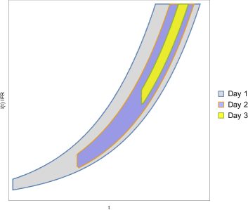
Figure 1: A scheme for the successive improvement of the predicted ${\cal D}(t)$ with successive days’ data on $D(t)$. Each day, the observed value of $D(t)$ is extrapolated back to the initial time to narrow the initial predicted interval of $I(t)$ through a Bayesian procedure.

Note that the very broad and skewed distributions of $T$ and ${\rm IFR\/}$ will give similarly broad and skewed distributions of $I(t)$. Here we suggest how to narrow these estimates progressively. Any knowledge of $I(t)$ gives a prediction of $I(t^{\prime})$ at a future date $t^{\prime}$. Uncertainties in $I(t)$ expand into larger uncertainties in $I(t^{\prime})$ due to exponential growth. However, the number of fatalities up to date $t^{\prime}$, i.e.. $D(t^{\prime})$, is directly observable. A time series for $D(t^{\prime})$ allows us to estimate $\tau$ directly. Furthermore, with each day’s data on fatalities, one can run the evolution backwards to rule out some of the uncertainty in the starting prediction $I(t)$ on 30 March. This means that the prediction for ${\cal D}(t^{\prime})=I(t^{\prime})\times{\rm IFR\/}$ further in the future is narrowed down. We show this inference procedure schematically in Figure 1. As the allowed range of the initial $I(t)$ successively narrows, one also narrows the allowed range of $T$ and ${\rm IFR\/}$ through a Bayesian inference paradigm.

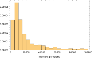
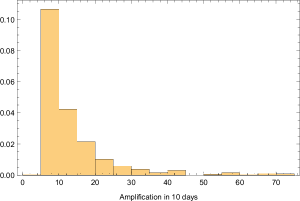
Figure 2: We show the probability distraction of the ratio $I(t)/D(t)$ (histogram on the left) and ${\cal D}(t+10)/D(10)$ (histogram on the right) in scenario B. The 95% confidence limit from the distribution on the left is the estimate quoted in eq. (5).

There are statistical uncertainties in the parameters $T$ and ${\rm CFR\/}$. We have combined them through a random Monte Carlo sampling using the probability distribution functions defined above. We implemented the Monte Carlo in Mathematica. The use of eq. (5) to make estimates of $I(t)$, and the future values $I(t^{\prime})$ and $D(t^{\prime})$, then gives a statistical distribution of these quantities. These are implemented in the same Monte Carlo estimator. The basic result is for the amplification factor, $I(t)/D(t)$, which we obtain with this numerical estimate,

$$I(t)=\begin{cases}\left(460\;{\rm to}\;9,700\right)\times D(t)&{\rm for\ scenario\ A}\\ \left(2,700\;{\rm to}\;3,80,000\right)\times D(t)&{\rm for\ scenario\ B}\\ \end{cases}$$ (5)

The ranges given here are 95% CL, and have been rounded to two significant digits. The median values are 1,500 in scenario A and 12,000 in scenario B.

We tested the effect of changing the skewness of the distribution by replacing the shifted Exponential distributions in eq. (2) and eq. (3) by Gamma distributions tuned so as to reproduce the same means and variances. However, the Gamma distributions then have smaller skewness.

$$I(t)=\begin{cases}\left(440\;{\rm to}\;7,700\right)\times D(t)&{\rm for\ scenario\ A}\\ \left(1,800\;{\rm to}\;2,00,000\right)\times D(t)&{\rm for\ scenario\ B}\\ \end{cases}$$ (6)

The medians are 1,600 in scenario A and 15,000 in scenario B. One sees that the medians and lower limits of the 95% CL change by relatively small amounts, whereas the upper limits are quite different.

Geographical Cluster	D(30/3)	Scenario A			Scenario B
		I(30/3)	$\cal D$(10/4)	$\cal D$(19/4)	I(30/3)	$\cal D$(10/4)	$\cal D$(19/4)
Mumbai-Navi Mumbai-Pune	8	3,700 – 77,000	18 – 61	39 – 380	22,000 – 3,00,000	42 – 470	189 – 18,000
Indore-Ujjain	6	2,800 – 58,000	13 – 46	29 – 290	16,000 – 2,30,000	32 – 350	140 – 14,000
Ahmbedabad-Bhavnagar	5	2,300 – 48,000	11 – 38	24 – 240	14,000 – 1,90,000	26 – 290	120 – 11,000
Kolkata-Howrah	2	930 – 19,000	5 – 15	10 – 96	5,400 – 7,50,000	10 – 120	47 – 4,600
Karnataka North	2	930 – 19,000	5 – 15	10 – 96	5,400 – 7,50,000	10 – 120	47 – 4,600

Table 1: Clusters of outbreaks, the number of reported fatalities up to March 30, the number of infected persons inferred from this up to 30 March, and the projected number of fatalities by 10 and 19 April in two different scenarios. All ranges quoted are 95% confidence limits and have been rounded to two significant digits. Scenario A has doubling time $\tau=10$ days, and in Scenario B $\tau=5$ days. The projected number of fatalities, $\cal D$, provides observational tests of the model. Note that the distributions are very skewed and that the median lies close to the lower limit of the very large 95% CL.

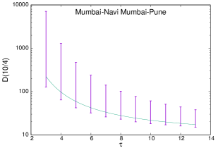
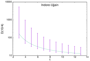
Figure 3: The 95% CL prediction for fatality counts ${\cal D}=I\times{\rm IFR\/}$ on 10 April for different values of $\tau$ are shown as the vertical lines. The continuous line joins the medians of these distributions. The plot on the left is for the Mumbai-Navi Mumbai-Pune hot-spot and that on the right for the Indore-Ujjain hot-spot.

We list the COVID-19 hot-spots in Table 1 along with estimates of $I$ and $\cal D$ on various dates for each in the two different scenarios defined earlier. We emphasize that different geographical locations may have different doubling times, so both scenarios may be relevant. These are our major results. For later use we also show in Figure 3 the 95% CL predictions for $\cal D$ on 10 April in two different hot-spots in Scenario B. Any limits that we can extract on disease and epidemiological parameters would help us to plan ahead for the kind of demands that may be put on medical facilities in the near future.

IV Discussion

From the data on the geographical distribution of fatalities in India, we identified four possible hot-spots for COVID-19. The clustering of fatalities into hot-spots is an indication that there is perhaps no general spread of the epidemic through the country, and gives hope for partial removal of lock-down if the situation does not change.

We used the simple statistical estimator given in eq. (4) to make a prediction for the total number of infections in each of these hot-spots on 30 March, in two scenarios. Estimating $I(t)$ is important, especially since there is a good chance that the part of this population which is pre-symptomatic, non-symptomatic, or has sub-clinical symptoms are all able to communicate the disease to others.

Our predictions are exhibited in Table 1. Note that the 95% CL spans an enormous range, due to the spread in the input parameters, mainly the time interval between infection and death. Note that the distribution of $I(t)$ is very skew, and the median is close to the lower end of the 95% CL. In Scenario B, the upper end of the 95% CL is more than 1% of the population of Mumbai. We consider this highly unlikely, although statistically possible. We have outlined a procedure refine these estimates by incorporating daily data progressively into the computation.

Given the very large values of $I(t)$ which the model predicts, medical professionals may legitimately ask whether one sees so many respiratory cases arriving in hospitals. Note however, that a very large fraction are likely to be either asymptomatic, or exhibit sub clinical symptoms. In fact ifr simultaneously reports ${\rm IFR\/}$ and the fraction of infected individuals who are hospitalized, $H$. This ratio, averaged over the population is reported to be in the range $H=2$–4%. In Scenario B, therefore one may expect 440–12,000 people to arrive in a hospital. Even among these, some may not be able to consult a physician during a lock-down. Nevertheless, current experience strongly disfavours the upper end of this 95% CL range. One recalls again, that the median is close to the lower end. This estimate again emphasizes how important it is to narrow the range of prediction from the model.

We are able to perform another simple estimate from these numbers. The case fatality ratio, ${\rm CFR\/}$, is defined as the number of fatalities divided by the number of cases tested. Assuming that the tests are largely done on the people who arrive at a hospital, one can see that

$${\rm CFR\/}\approx\frac{D(t)}{HI(t)}=\frac{{\rm IFR\/}}{H}.$$ (7)

With ${\rm IFR\/}=0.657$% and $H=2$–4%, we find ${\rm CFR\/}=0.16$–0.33, i.e., in the range of 16% to 33%. This is precisely in the range that is seen in the current data for India. This also means that the current policy for testing is likely to be catching most cases which need to be hospitalized. One hopes that with the decision to administer the faster serum test, it might become possible to sample the larger population more effectively.

Finally we point out that there is a strong age structure to all the model parameters, which we have ignored. This we plan to do in future. Along with the planned Bayesian narrowing of the parameter space of COVID-19 pathology and epidemiology, this would provide valuable inputs for more detailed models which can be used to inform future policy.

V Acknowledgements

The authors would like to thank Sandhya Koushika, Gautam Menon, and Rahul Siddharthan for crucial inputs, and many members of the ISRC (Indian Scientists’ Response to COVID-19) mailing list for discussions.

References

- (1) N. van Doremalen, et al., Aerosol and Surface Stability of SARS-CoV-2 as Compared with SARS-CoV-1 New England J. Med. (2020) [DOI: 10.1056/NEJMc2004973]
- (2) S. A. Lauer, K. H. Grantz, Q. Bi, F. K. Jones, Q. Zheng, H. R. Meredith, A. S. Azman, and N. G. Reich, The Incubation Period of Coronavirus Disease 2019 (COVID-19) from Publicly Reported Confirmed Cases: Estimation and Application, Ann. Int. Med. (2020) [preprint version doi:10.1101/2020.02.02.20020016]
- (3) L. Lan, D. Xu, G. Ye, C. Xia, S. Wang, Y. Li, and H. Xu, Positive RT-PCR Test Results in Patients Recovered from COVID-19, JAMA (2020)
- (4) Y. Liu, A. A. Gayle, A. Wilder-Smith, and J. Rocklöv, The reproductive number of COVID-19 is higher compared to SARS Coronavirus, J. Travel Medicine, 27, taaa021, 2020. [https://doi.org/10.1093/jtm/taaa021]
- (5) J. Rocklöv, H. Sjödin, A. Wilder-Smith, COVID-19 outbreak on the Diamond Princess cruise ship: estimating the epidemic potential and the effectiveness of public health countermeasures, J. Travel Medicine, 27, taaa030, 2020. [https://doi.org/10.1093/jtm/taaa030]
- (6) http://censusindia.gov.in/2011-Common/CensusData2011.html
- (7) Z. Wu and J. M. McGoogan, Characteristics of and Important Lessons from the Coronavirus Disease 2019 (COVID-19) Outbreak in China, JAMA, (2020). [doi:10.1001/jama.2020.2648]
- (8) R. Verity, et al., Estimates of the severity of Coronavirus disease 2019: a model based analysis, Lancet Infectious Diseases, (2020) [https://doi.org/10.1016/S1473-3099(20)30243-7]
- (9) Q. Ruan, K. Yang, W. Wang, L. Jiang and J. Song, Clinical predictors of mortality due to COVID-19 base on an analysis of data of 150 patients from Wuhan, China, Intensive Care Med. (2020). [https://doi.org/10.1007/s00134-020-05991-x]
- (10) M. Lipsitch et al., Potential Biases in Estimating Absolute and Relative Case-Fatality Risks during Outbreaks, PLoS Negl. Trop. Dis. 9(7): e0003846 [doi:10.1371/journal.pntd.0003846]
- (11) https://www.mohfw.gov.in/index.html
- (12) https://en.wikipedia.org/wiki/Timeline_of_the_2020_coronavirus_pandemic_in_India