Comment on “The negative flow of probability”

Abstract

The left-to-right motion of a free quantum Gaussian wave packet can be accompanied by the right-to-left flow of the probability density, the effect recently studied by Villanueva [Am. J. Phys. 88, 325 (2020)]. Using the Wigner representation of the wave packet, we analyze the effect in phase space, and demonstrate that its physical origin is rooted in classical mechanics.

In a recent paper Villanueva (2020), Villanueva has explored a seemingly paradoxical effect associated with the motion of a free quantum particle. The particle state is represented by a Gaussian wave packet:

$$\psi(x,t)=\exp\left(\frac{i}{\hbar}\alpha_{t}(x-x_{t})^{2}+\frac{i}{\hbar}p_{0}(x-x_{t})+\frac{i}{\hbar}\gamma_{t}\right)\,,$$ (1)

where $x$ and $t$ are the position and time variables, respectively. Here,

$$x_{t}=x_{0}+\frac{p_{0}t}{m}\,,$$ (2)

is the wave packet center at time $t$, with $x_{0}$ and $p_{0}$ being the initial mean position and momentum, respectively; $m$ is the particle mass. The complex-valued function $\alpha_{t}$ is defined as

$$\frac{1}{\alpha_{t}}=\frac{1}{\alpha_{0}}+\frac{2t}{m}\,,$$ (3)

and controls the wave packet spread,

$$(\Delta x)_{t}\equiv\sqrt{\langle x^{2}\rangle_{t}-\langle x\rangle_{t}^{2}}=\frac{1}{2}\sqrt{\frac{\hbar}{\operatorname{Im}\alpha_{t}}}\,,$$

along with position-momentum correlations. Its initial value, $\alpha_{0}$, must satisfy $\operatorname{Im}\alpha_{0}>0$ for the wave packet to be normalizable. Finally, the complex-valued function $\gamma_{t}$ encapsulates both the normalization constant and global phase; the imaginary part of $\gamma_{t}$ is related to that of $\alpha_{t}$ via

$$\exp\left(-\frac{2\operatorname{Im}\gamma_{t}}{\hbar}\right)=\sqrt{\frac{2\operatorname{Im}\alpha_{t}}{\pi\hbar}}\,.$$ (4)

The wave function $\psi(x,t)$ satisfies the free particle Schrödinger equation:

$$i\hbar\frac{\partial\psi}{\partial t}=-\frac{\hbar^{2}}{2m}\frac{\partial^{2}\psi}{\partial x^{2}}\,.$$ (5)

The effect addressed by Villanueva can be summarized as follows. Let $q$ be some fixed point on the $x$-axis, and consider the scenario in which

$$q-x_{0}\gg(\Delta x)_{0}\qquad\text{and}\qquad p_{0}>0\,.$$

In other words, the initial wave packet is localized (almost entirely) on the left of $q$ and is moving to the right. Naively, one might think that, as the wave packet approaches the point $q$ from the left (that is, as long as $x_{t}<q$), the probability of finding the particle in the region $x>q$, namely

$$\Pi(t)=\int_{q}^{+\infty}dx\,|\psi(x,t)|^{2}\,,$$ (6)

grows monotonically with time, i.e. one might expect that $\frac{d}{dt}\Pi(t)>0$ for $0<t<t_{\text{cl}}\equiv\frac{m(q-x_{0})}{p_{0}}$. However, as Villanueva demonstrates, this naive intuition can be false: If the value of the parameter $\alpha_{0}$ is such that

$$\operatorname{Re}\alpha_{t}<-\frac{p_{0}}{2(q-x_{t})}\,,$$ (7)

at an instant $t<t_{\text{cl}}$, then the probability $\Pi(t)$ appears to be decreasing,

$$\frac{d}{dt}\Pi(t)<0\,.$$

Here we point out that, if considered in phase space, the above effect has a simple intuitive explanation. In fact, the effect is rooted in classical mechanics: The same negative flow of probability takes place in an ensemble of free classical particles with an appropriate Gaussian distribution of positions and momenta. We also present a phase-space-based derivation of condition (7).

Let us regard the motion of a free particle, described in the Schrödinger picture by the wave function $\psi(x,t)$, as the time evolution of the Wigner phase-space (quasiprobability) density Snygg (1980); Case (2008)

$$W(x,p,t)=\frac{1}{\pi\hbar}\int_{-\infty}^{+\infty}dy\,e^{-i2py/\hbar}\psi(x+y,t)\psi^{*}(x-y,t)\,.$$

The reader is referred to review articles Snygg (1980); Case (2008) for a discussion of many fascinating properties of the Wigner density. Here, we only state the following two properties, particularly relevant to the present discussion. First, the time evolution of $W(x,p,t)$ in free space is governed by

$$W(x,p,t)=W(x-pt/m,p,0)\,.$$ (8)

This equation is the phase-space representation to the free-particle Schrödinger equation (5). Second, in terms of the Wigner function, the probability of finding the particle in the region $x>q$ reads

$$\Pi(t)=\int_{q}^{+\infty}dx\int_{-\infty}^{+\infty}dp\,W(x,p,t)\,.$$ (9)

This is the phase-space representation of Eq. (6).

Substituting $\psi(x,t)$, given by Eq. (1), into Eq. (8), performing the integration, and using identity (4), we obtain

$$W(x,p,t)=\frac{1}{\pi\hbar}\exp\left(-\frac{2\widetilde{x}^{2}\operatorname{Im}\alpha_{t}}{\hbar}-\frac{\left(\widetilde{p}-2\widetilde{x}\operatorname{Re}\alpha_{t}\right)^{2}}{2\hbar\operatorname{Im}\alpha_{t}}\right)\,,$$ (10)

where

$$\widetilde{x}=x-x_{t}\qquad\text{and}\qquad\widetilde{p}=p-p_{0}$$

are, respectively, the particle position and momentum measured relative to their mean values. The Wigner function (10) is positive at all times, $W(x,p,t)>0$.

Now comes an important (and well known) argument. Imagine an ensemble of $N$ free noninteracting classical particles of mass $m$. We are interested in the limit of large $N$. Let $NW_{\text{cl}}(x,p,t)$ be the number density of the particles at the phase-space point $(x,p)$ at time $t$. So, $W_{\text{cl}}(x,p,t)$ is the probability density for a given particle to be found at $(x,p)$ at time $t$. Since the momentum of a free particle is conserved, the time evolution of $W_{\text{cl}}$ is given by

$$W_{\text{cl}}(x,p,t)=W_{\text{cl}}(x-pt/m,p,0)\,.$$ (11)

The number of particles in the region $x>q$ at time $t$ equals $N\Pi_{\text{cl}}(t)$, where

$$\Pi_{\text{cl}}(t)=\int_{q}^{+\infty}dx\int_{-\infty}^{+\infty}dp\,W_{\text{cl}}(x,p,t)$$ (12)

represents the probability for a given particle to satisfy $x>q$ at time $t$. Observe that Eqs. (8) and (9) for the Wigner function $W$ of a quantum particle are identical to Eqs. (11) and (12) for the classical phase-space probability density $W_{\text{cl}}$, respectively . It then immediately follows that

$$\Pi(t)=\Pi_{\text{cl}}(t)\,,$$ (13)

provided that $W(x,p,0)=W_{\text{cl}}(x,p,0)$. In general Snygg (1980); Case (2008), the set of all possible Wigner functions $W(x,p,0)$ is not the same as the set of all possible classical probability densities $W_{\text{cl}}(x,p,0)$. For example, $W(x,p,0)$ can have negative values, whereas $W_{\text{cl}}(x,p,0)$ is nonnegative by construction; on the other hand, the value of $W_{\text{cl}}(x,p,0)$ can in principle be arbitrarily large, whereas $|W(x,p,0)|\leq 1/\pi\hbar$ for all $x$ and $p$. However, the Wigner function $W$ representing a Gaussian wave packet is everywhere positive, Eq. (10), and therefore can be regarded as a valid classical probability density $W_{\text{cl}}$. This guaranties that the behavior of $\Pi(t)$ for a Gaussian quantum state, described by an initial Wigner function $W(x,p,0)$, is identical to the behavior of $\Pi_{\text{cl}}(t)$ for an ensemble of free classical particles, initially distributed in accordance with the phase-space density $W_{\text{cl}}(x,p,0)=W(x,p,0)$. In particular, this means that the negative flow of probability addressed by Villanueva Villanueva (2020) is essentially a classical-mechanical effect.

We now present a phase-space interpretation of the effect. For the discussion below, it is important to introduce dimensionless versions of the position, momentum, and time variables. This requires defining a natural length scale $L$. We achieve this by noticing that, according to Eq. (3), the quantity $\operatorname{Im}\left(1/\alpha_{t}\right)=-(\operatorname{Im}\alpha_{t})/|\alpha_{t}|^{2}$ does not depend on time, i.e. $\operatorname{Im}\left(1/\alpha_{t}\right)=\operatorname{Im}\left(1/\alpha_{0}\right)$. Thus, $L$ can be defined as

$$L^{2}\equiv\frac{\hbar}{2}\frac{\operatorname{Im}\alpha_{t}}{|\alpha_{t}|^{2}}=\frac{\hbar}{2}\frac{\operatorname{Im}\alpha_{0}}{|\alpha_{0}|^{2}}\,.$$ (14)

Subsequently, we introduce dimensionless positions

$$\xi=\frac{x}{L}\,,\qquad\xi_{0}=\frac{x_{0}}{L}\,,\qquad\delta=\frac{q}{L}\,,$$ (15)

dimensionless momenta

$$\eta=\frac{p}{\hbar/L}\,,\qquad\eta_{0}=\frac{p_{0}}{\hbar/L}\,,$$ (16)

dimensionless time

$$\tau=\frac{t}{mL^{2}/\hbar}\,,$$

and dimensionless (quasi)probability density

$$\Omega(\xi,\eta,\tau)=\frac{W(x,p,t)}{1/\hbar}\,.$$

A straightforward calculation yields the following dimensionless version of the Wigner function (10):

$$\Omega(\xi,\eta,\tau)=\frac{1}{\pi}e^{-\left(\widetilde{\xi}-\epsilon_{\tau}\widetilde{\eta}\right)^{2}-\widetilde{\eta}^{2}}\,,$$ (17)

where

$$\epsilon_{\tau}=\left.\frac{\operatorname{Re}\alpha_{t}}{\operatorname{Im}\alpha_{t}}\,\right|_{t=\frac{mL^{2}}{\hbar}\tau}\,,$$ (18)

and

$$\widetilde{\xi}=\xi-\xi_{\tau}\qquad\text{and}\qquad\widetilde{\eta}=\eta-\eta_{0}\,.$$ (19)

The time dependence of the dimensionless Wigner function is specified by

$$\xi_{\tau}=\xi_{0}+\eta_{0}\tau\,,$$ (20)

cf. Eq. (2), and

$$\epsilon_{\tau}=\epsilon_{0}+\tau\,,$$ (21)

cf. Eq. (3), where $\epsilon_{0}=\operatorname{Re}\alpha_{0}/\operatorname{Im}\alpha_{0}$. It is easy to check that the dimensionless Wigner function satisfies the free particle evolution equation

$$\Omega(\xi,\eta,\tau)=\Omega(\xi-\eta\tau,\eta,0)\,,$$ (22)

cf. Eqs. (8) and (11), and that the probability of finding the particle in the region $\xi>\delta$ (or $x>q$) at time $\tau$ (or $t$) is given by

$$\Pi(\tau)=\int_{\delta}^{+\infty}d\xi\int_{-\infty}^{+\infty}d\eta\,\Omega(\xi,\eta,\tau)\,,$$

cf. Eqs. (9) and (12).

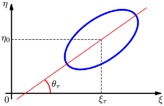
Figure 1: An elliptical curve in phase space on which the Wigner function $\Omega(\xi,\eta,\tau)$ has a constant value. The ellipse becomes a circle when $\epsilon_{\tau}=0$; this corresponds to a minimal uncertainty state.

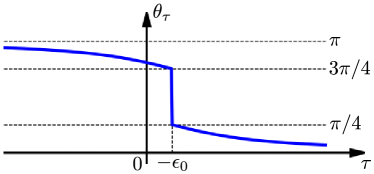
Figure 2: Angle $\theta_{\tau}$, illustrated in Fig. 1, as a function of time $\tau$. At $\tau=-\epsilon_{0}$, the particle is in a minimal uncertainty state, for which $\theta_{\tau}$ is not defined.

Equations (17), (19), (20), and (21) provide the complete description of the motion of a free Gaussian wave packet. At time $\tau$, the wave packet is parametrized by three dimensionless real numbers: $\xi_{\tau}$, $\eta_{0}$, and $\epsilon_{\tau}$. Figure 1 shows a phase-space curve of a constant value of $\Omega(\xi,\eta,\tau)$. The curve is an ellipse centered at $(\xi_{\tau},\eta_{0})$. It is easy to show (see Appendix A) that the angle between the major axis of the ellipse and the $\xi$-axis is given by

$$\theta_{\tau}=\left\{\begin{array}[]{ll}\displaystyle\frac{1}{2}\arctan\frac{2}{\epsilon_{\tau}}&\text{if}\quad\epsilon_{\tau}>0\\[11.38092pt] \displaystyle\pi+\frac{1}{2}\arctan\frac{2}{\epsilon_{\tau}}&\text{if}\quad\epsilon_{\tau}<0\end{array}\right.\,.$$ (23)

The angle $\theta_{\tau}$ decreases monotonically from $\pi$ to $0$ as time $\tau$ increases from $-\infty$ to $+\infty$. This is shown in Fig. 2. According to Eq. (21), $\epsilon_{\tau}=0$ when time $\tau=-\epsilon_{0}$. At this instant, the Wigner function representing the wave packet reads

$$\Omega(\xi,\eta,-\epsilon_{0})=\frac{1}{\pi}e^{-\tilde{\xi}^{2}-\tilde{\eta}^{2}}\,.$$

This is a minimal uncertainty state. The phase-space contour lines representing minimal uncertainty states are circles, and so the angle $\theta_{\tau}$ is not defined at $\tau=-\epsilon_{0}$. In Fig. 2, the value of $\epsilon_{0}$ is chosen to be negative.

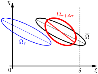
Figure 3: The time evolution of the Wigner function from $\Omega_{\tau}\equiv\Omega(\xi,\eta,\tau)$ to $\Omega_{\tau+\Delta\tau}\equiv\Omega(\xi,\eta,\tau+\Delta\tau)$ as a sequence two consecutive transformations: $\Omega_{\tau}\to\overline{\Omega}$ and $\overline{\Omega}\to\Omega_{\tau+\Delta\tau}$. See the text for details. Each Wigner function is represented by an elliptical contour line, along with the corresponding major axis. The left boundary of the spatial region $\xi>\delta$ is shown with a dashed line.

The time evolution of the Wigner function during the time interval between $\tau$ and $\tau+\Delta\tau$, i.e.

$$\Omega(\xi,\eta,\tau)\quad\to\quad\Omega(\xi,\eta,\tau+\Delta\tau)=\Omega(\xi-\eta\Delta\tau,\eta,\tau)\,,$$

can be viewed as the result of two consecutive transformations, both illustrated in Fig. 3. The first transformation is a rigid shift of the Wigner distribution along the $\xi$-axis by $\eta_{0}\Delta\tau$:

$$\Omega(\xi,\eta,\tau)\quad\to\quad\overline{\Omega}(\xi,\eta)=\Omega(\xi-\eta_{0}\Delta\tau,\eta,\tau)\,.$$ (24)

The second transformation is a simple shear leaving the distribution center unchanged:

$$\overline{\Omega}(\xi,\eta)\quad\to\quad\Omega(\xi,\eta,\tau+\Delta\tau)=\overline{\Omega}\big{(}\xi-(\eta-\eta_{0})\Delta\tau,\eta\big{)}\,.$$ (25)

The change in the Wigner density $\Delta\Omega$ during the time interval between $\tau$ and $\tau+\Delta\tau$ is given by

$$\Delta\Omega \equiv\Omega(\xi,\eta,\tau+\Delta\tau)-\Omega(\xi,\eta,\tau)$$

$$=(\Delta\Omega)_{\text{shift}}+(\Delta\Omega)_{\text{shear}}\,,$$

where

$$(\Delta\Omega)_{\text{shift}}=\overline{\Omega}(\xi,\eta)-\Omega(\xi,\eta,\tau)$$ (26)

is the change due to the shift transformation, and

$$(\Delta\Omega)_{\text{shear}}=\Omega(\xi,\eta,\tau+\Delta\tau)-\overline{\Omega}(\xi,\eta)$$ (27)

is the change due to the shear transformation. Consequently, the corresponding change in the probability of finding the particle in the region $\xi>\delta$ is

$$\Delta\Pi \equiv\Pi(\tau+\Delta\tau)-\Pi(\tau)$$

$$=\int_{\delta}^{+\infty}d\xi\int_{-\infty}^{+\infty}d\eta\,\Delta\Omega$$

$$=(\Delta\Pi)_{\text{shift}}+(\Delta\Pi)_{\text{shear}}\,,$$

where

$$(\Delta\Pi)_{\text{shift}}=\int_{\delta}^{+\infty}d\xi\int_{-\infty}^{+\infty}d\eta\,(\Delta\Omega)_{\text{shift}}$$ (28)

and

$$(\Delta\Pi)_{\text{shear}}=\int_{\delta}^{+\infty}d\xi\int_{-\infty}^{+\infty}d\eta\,(\Delta\Omega)_{\text{shear}}\,.$$ (29)

It is straightforward to show (see Appendix B) that, in the limit of small $\Delta\tau$,

$$(\Delta\Pi)_{\text{shift}}=\eta_{0}\Delta\tau\int_{-\infty}^{+\infty}d\eta\,\Omega(\delta,\eta,\tau)$$ (30)

and

$$(\Delta\Pi)_{\text{shear}}=\Delta\tau\int_{-\infty}^{+\infty}d\eta\,(\eta-\eta_{0})\Omega(\delta,\eta,\tau)\,.$$ (31)

In the case of the Wigner function $\Omega$ given by Eq. (17), the probability change due to the shift transformation is always positive:

$$(\Delta\Pi)_{\text{shift}}>0\,.$$

This follows directly from the fact that $\Omega(\xi,\eta,\tau)>0$. However, the probability change due to the shear transformation, $(\Delta\Pi)_{\text{shear}}$, can be negative for some values of the wave packet parameters. Figure 3 provides an example of the situation in which $(\Delta\Pi)_{\text{shear}}<0$; it is clear that $\epsilon_{\tau}<0$ (or, equivalently, $\theta_{\tau}>3\pi/4$) is a necessary condition for $(\Delta\Pi)_{\text{shear}}$ to be negative. The negative flow of the net probability, $\Delta\Pi<0$, occurs if and only if

$$(\Delta\Pi)_{\text{shear}}<-(\Delta\Pi)_{\text{shift}}\,.$$ (32)

This condition is the phase-space equivalent of Eq. (7).

In order to explicitly recover Eq. (7) from Eq. (32), we substitute Eq. (17) into Eqs. (30) and (31), and evaluate the corresponding momentum integrals. This yields (see Appendix B)

$$(\Delta\Pi)_{\text{shift}}=\frac{\eta_{0}\Delta\tau}{\sqrt{\pi\left(1+\epsilon_{\tau}^{2}\right)}}\exp\left[-\frac{(\delta-\xi_{\tau})^{2}}{1+\epsilon_{\tau}^{2}}\right]$$ (33)

and

$$(\Delta\Pi)_{\text{shear}}=\frac{\epsilon_{\tau}(\delta-\xi_{\tau})\Delta\tau}{\sqrt{\pi\left(1+\epsilon_{\tau}^{2}\right)^{3}}}\exp\left[-\frac{(\delta-\xi_{\tau})^{2}}{1+\epsilon_{\tau}^{2}}\right]\,.$$ (34)

Substituting these expressions into Eq. (32), we obtain

$$\frac{\epsilon_{\tau}}{1+\epsilon_{\tau}^{2}}<-\frac{\eta_{0}}{\delta-\xi_{\tau}}\,.$$ (35)

Using the rescaling transformations (14), (15), (16), and (18), it can be easily verified that Eq. (35) is the dimensionless version of the negative probability flow condition (7). The geometrical meaning of this condition is discussed in Appendix C.

In summary, we have shown that the effect of the negative probability flow, studied by Villanueva Villanueva (2020), has an intuitive explanation when considered in phase space. The effect is classical-mechanical in nature, and occurs not only for a free quantum particle with a Gaussian wave function, but also for an ensemble of free classical particles with a Gaussian distribution of positions and momenta.

Appendix A Derivation of Eq. (23)

There are many ways to derive Eq. (23). Here we adopt a direct one. It follows from Eq. (17) that phase-space points $(\xi,\eta)$ corresponding to the same value of $\Omega(\xi,\eta,\tau)$ lie on the ellipse

$$\left(\widetilde{\xi}-\epsilon_{\tau}\widetilde{\eta}\right)^{2}+\widetilde{\eta}^{2}=C\,,$$

where $C>0$ is a constant. In polar coordinates,

$$\widetilde{\xi}=r\cos\theta\,,\qquad\widetilde{\eta}=r\sin\theta\,,$$

the ellipse equation takes the form

$$r^{2}=\frac{C}{1-\epsilon_{\tau}\sin 2\theta+\epsilon_{\tau}^{2}\sin^{2}\theta}\,.$$

The angle $\theta=\theta_{\tau}$ is the one that maximizes $r$, and therefore satisfies the equation

$$\frac{dr^{2}}{d\theta}=0\,,$$

which is equivalent to

$$2\epsilon_{\tau}\cos 2\theta-\epsilon_{\tau}^{2}\sin 2\theta=0\,.$$

For $\epsilon_{\tau}\not=0$, this reduces to

$$\tan 2\theta=\frac{2}{\epsilon_{\tau}}\,.$$

On the interval $0<\theta<\pi$, this equation has two solutions: (i) the solution given by Eq. (23), and (ii) the one representing the orthogonal direction, i.e.

$$\theta_{\tau}^{\perp}=\frac{\pi}{2}+\frac{1}{2}\arctan\frac{2}{\epsilon_{\tau}}\,.$$

A straightforward evaluation of $\frac{d^{2}r}{d\theta^{2}}$ shows that it is the solution given by Eq. (23) that maximizes $r$.

Appendix B Derivation of Eqs. (30), (31), (33), (34)

We first derive Eqs. (30) and (31). From Eqs. (26) and (24), we have

$$(\Delta\Omega)_{\text{shift}} =\Omega(\xi-\eta_{0}\Delta\tau,\eta,\tau)-\Omega(\xi,\eta,\tau)$$

$$=-\eta_{0}\Delta\tau\frac{\partial\Omega(\xi,\eta,\tau)}{\partial\xi}+O\left(\Delta\tau^{2}\right)\,.$$

Substituting this into Eq. (28), and only keeping the leading order term in $\Delta\tau$, we obtain

$$(\Delta\Pi)_{\text{shift}} =-\eta_{0}\Delta\tau\int_{-\infty}^{+\infty}d\eta\int_{\delta}^{+\infty}d\xi\,\frac{\partial\Omega(\xi,\eta,\tau)}{\partial\xi}$$

$$=\eta_{0}\Delta\tau\int_{-\infty}^{+\infty}d\eta\,\Omega(\delta,\eta,\tau)\,,$$

where we have taken into account the fact that $\Omega(\xi,\eta,\tau)\to 0$ as $\xi\to\infty$. Similarly, from Eqs. (27), (25), and (24), we have

$$(\Delta\Omega)_{\text{shear}} =\overline{\Omega}\big{(}\xi-(\eta-\eta_{0})\Delta,\eta\big{)}-\overline{\Omega}(\xi,\eta)$$

$$=-(\eta-\eta_{0})\Delta\tau\frac{\partial\overline{\Omega}(\xi,\eta)}{\partial\xi}+O\left(\Delta\tau^{2}\right)$$

$$=-(\eta-\eta_{0})\Delta\tau\frac{\partial}{\partial\xi}\Omega(\xi-\eta_{0}\Delta\tau,\eta,\tau)+O\left(\Delta\tau^{2}\right)$$

$$=-(\eta-\eta_{0})\Delta\tau\frac{\partial\Omega(\xi,\eta,\tau)}{\partial\xi}+O\left(\Delta\tau^{2}\right)\,.$$

Substituting this into Eq. (29), and only keeping the leading order term in $\Delta\tau$, we obtain

$$(\Delta\Pi)_{\text{shear}} =-\Delta\tau\int_{-\infty}^{+\infty}d\eta\,(\eta-\eta_{0})\int_{\delta}^{+\infty}d\xi\,\frac{\partial\Omega(\xi,\eta,\tau)}{\partial\xi}$$

$$=\Delta\tau\int_{-\infty}^{+\infty}d\eta\,(\eta-\eta_{0})\Omega(\delta,\eta,\tau)\,.$$

Now we derive Eq. (33) and (34). According to Eq. (17), $\Omega$ can be written as

$$\Omega(\xi,\eta,\tau)=\frac{1}{\pi}e^{-a\eta^{2}+2b\eta-c}$$

with

$$a=1+\epsilon_{\tau}^{2}\,,$$

$$b=\left(1+\epsilon_{\tau}^{2}\right)\eta_{0}+\epsilon_{\tau}(\delta-\xi_{\tau})\,,$$

$$c=(\delta-\xi_{\tau}+\epsilon_{\tau}\eta_{0})^{2}+\eta_{0}^{2}\,.$$

Hence,

$$\int_{-\infty}^{+\infty}d\eta\,\Omega(\delta,\eta,\tau)=\frac{1}{\pi}\int_{-\infty}^{+\infty}d\eta\,e^{-a\eta^{2}+2b\eta-c}=\frac{e^{b^{2}/a-c}}{\sqrt{\pi a}}\,.$$

Since

$$\frac{b^{2}}{a}-c=-\frac{(\delta-\xi_{\tau})^{2}}{1+\epsilon_{\tau}^{2}}\,,$$

we get

$$\int_{-\infty}^{+\infty}d\eta\,\Omega(\delta,\eta,\tau)=\frac{1}{\sqrt{\pi\left(1+\epsilon_{\tau}^{2}\right)}}\exp\left[-\frac{(\delta-\xi_{\tau})^{2}}{1+\epsilon_{\tau}^{2}}\right]\,,$$

which, in turn, leads to Eq. (33). Then,

$$\int_{-\infty}^{+\infty}d\eta\,\eta\Omega(\delta,\eta,\tau) =\frac{1}{\pi}\int_{-\infty}^{+\infty}d\eta\,\eta e^{-a\eta^{2}+2b\eta-c}$$

$$=\frac{b}{a}\frac{e^{b^{2}/a-c}}{\sqrt{\pi a}}\,,$$

and so

$$\int_{-\infty}^{+\infty}d\eta\,(\eta-\eta_{0}) \Omega(\delta,\eta,\tau)=(b-a\eta_{0})\frac{e^{b^{2}/a-c}}{\sqrt{\pi a^{3}}}$$

$$=\frac{\epsilon_{\tau}(\delta-\xi_{\tau})}{\sqrt{\pi\left(1+\epsilon_{\tau}^{2}\right)^{3}}}\exp\left[-\frac{(\delta-\xi_{\tau})^{2}}{1+\epsilon_{\tau}^{2}}\right]\,.$$

This yields Eq. (34).

Appendix C Geometrical meaning of Eq. (35)

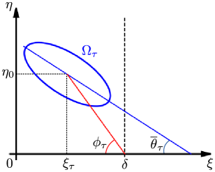
Figure 4: Angles $\overline{\theta}_{\tau}=\pi-\theta_{\tau}$ and $\phi_{\tau}$ for the Wigner function $\Omega_{\tau}\equiv\Omega(\xi,\eta,\tau)$.

Condition (35) determines the phase-space position and orientation of the Wigner function $\Omega(\xi,\eta,\tau)$ accompanied by negative probability flow at the point $\xi=\delta$. The geometrical meaning of this condition becomes clear if we rewrite Eq. (35) in terms of angles $\overline{\theta}_{\tau}=\pi-\theta_{\tau}$ and $\phi_{\tau}$, defined in Fig. 4. We have

$$\frac{\eta_{0}}{\delta-\xi_{\tau}}=\tan\phi_{\tau}>0$$

and, in view of Eq. (23),

$$\epsilon_{\tau}=\frac{2}{\tan 2\theta_{\tau}}=-\frac{2}{\tan 2\overline{\theta}_{\tau}}\,.$$

Substituting these two expressions into Eq. (35), we find that $\overline{\theta}_{\tau}$ must lie inside the interval $(0,\pi/4)$ and satisfy the inequality

$$\frac{\tan 2\overline{\theta}_{\tau}}{2}+\frac{2}{\tan 2\overline{\theta}_{\tau}}<\frac{1}{\tan\phi_{\tau}}\,.$$ (36)

This inequality is equivalent to Eq. (35).

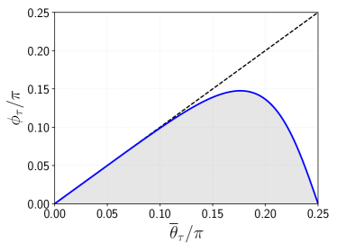
Figure 5: The shaded area shows the angles $\overline{\theta}_{\tau}$ and $\phi_{\tau}$ for which condition (36) is fulfilled. The dashed line corresponds to $\phi_{\tau}=\overline{\theta}_{\tau}$.

Figure 5 shows the set of angle pairs $(\overline{\theta}_{\tau},\phi_{\tau})$ fulfilling condition (36). The condition becomes especially simple in the limit of small $\overline{\theta}_{\tau}$: If $\overline{\theta}_{\tau}\ll 1$, then negative probability flow at $\xi=\delta$ occurs for $\phi_{\tau}<\overline{\theta}_{\tau}$.