Is the variance swap rate affine in the spot variance? Evidence from S&P500 data

Abstract

We empirically investigate the functional link between the variance swap rate and the spot variance. Using S&P500 data over the period 2006-2018, we find overwhelming empirical evidence supporting the affine link analytically found by Kallsen et al. (2011) in the context of exponentially affine stochastic volatility models. Tests on yearly subsamples suggest that exponentially mean-reverting variance models provide a good fit during periods of extreme volatility, while polynomial models, introduced in Cuchiero (2011), are suited for years characterized by more frequent price jumps.

C2, C12, C51, G12, G13.

1 Introduction

The class of the exponentially affine processes, introduced in the seminal paper by Duffie et al. (2000) and characterized by Filipovic (2001), has received large consensus in the quantitative finance literature, based on its main advantages in terms of analytical tractability and empirical flexibility. The classic example of an exponentially affine process, and the only one with continuous paths, is the CIR diffusion, see Cox et al. (1985). The related stochastic volatility model, studied by Heston (1993), is considered as a reference model by scholars and practitioners. Kallsen et al. (2011) have studied the valuation of options written on the quadratic variation of the asset price within the exponentially affine stochastic volatility framework. In particular, they have proved, analytically, the existence of an affine link between the expected cumulated variance, i.e., the variance swap rate, and the spot variance. Note that the class of stochastic volatility models considered in Kallsen et al. (2011) allows for jumps and leverage effects, but fails to include some popular stochastic volatility models, e.g., the models by Beckers (1980); Grasselli (2016); Hagan et al. (2002); Platen (1997). The variance swap is possibly the most plain vanilla contingent claim written on the realized variance. Indeed, it can be seen, to some extent, as the forward of the integrated variance of log-returns (see, for instance, Bernis et al. (2019); Carr and Sun (2007); Carr and Wu (2008); Filipovic et al. (2016); Jiao et al. (2019); Kallsen et al. (2011)). Volatility derivatives appear nowadays with a vast demand, especially after the global financial crisis of 2008, which induced large fluctuations in the volatility and other indicators of market stress. The large demand for volatility derivatives has resulted in a major increase in their liquidity, and thus in the reliability of their prices (see, for instance, Carr and Wu (2008)).

Based on the study by Kallsen et al. (2011), two natural questions arise: (i) could we analytically identify a wider class of models which admits an affine link between the variance swap rates and the spot variance? (ii) is it possible to test if empirical data satisfy a given link (e.g., affine, quadratic) between the variance swap rate and the unobservable spot variance? This paper contributes to answering both questions. With regard to question (i), we prove that a larger class of models exhibits a linear link between the variance swap rate and the spot variance, and we show that a quadratic (respectively, affine) link appears between the variance swap rate and the multidimensional stochastic process characterizing the model, in the presence (respectively, absence) of jumps, within the class of polynomial models (see Cuchiero (2011) and Cuchiero et al. (2012)). With regard to question (ii), we set up a simple testing procedure, based on Ordinary-Least-Squares (OLS), in which the unobservable spot variance is replaced with efficient Fourier estimates thereof. Then, we apply it to S&P500 empirical data over the period 2006-2018.

In particular, our first result is showing that a model exhibits the affine link between the variance swap rate and the spot variance if the stochastic differential equation satisfied by the latter is the sum of an affine drift and a zero-mean stochastic process. We term this class exponentially mean-reverting variance models. This class is fairly large. In fact, it contains not only exponentially affine processes with jumps (see, e.g., Bates (1996); Barndorff-Nielsen and Shephard (2001); Barndorff-Nielsen and Shephard (2002a); Duffie et al. (2003); Jiao et al. (2017, 2019)), but also, under suitable conditions (see Cuchiero et al. (2012); Ackerer et al. (2018)), polynomial processes. Moreover, it also contains some models based on the fractional Brownian motion, like the rough Heston model (see, for instance Bayer et al. (2016); El Euch et al. (2019); El Euch and Rosenbaum (2019); Gatheral et al. (2018)). However, it is worth noting that many popular models, e.g., the CEV model (Beckers (1980)), the SABR model (Hagan et al. (2002)), the $3/2$ and $4/2$ models (Platen (1997); Grasselli (2016)), fail to verify the affine link (see, for instance, the analysis in Section 4 of Jarrow et al. (2013) for the 3/2 model). Further, we consider the class of stochastic volatility models based on polynomial processes, introduced in Cuchiero (2011) and Cuchiero et al. (2012). The exponentially affine models by Kallsen et al. (2011), which exhibit an affine link between the variance swap rate and the spot variance, are included in the polynomial class, as a special case, see Example 3.1 in Cuchiero et al. (2012). In the polynomial framework, we prove the existence, in the presence of jumps, of a quadratic correction in the link between the theoretical variance swap rate and the spot variance.

In the financial market, traded variance swaps are actually written on the realized variance, that is the finite sum of squared log-returns sampled over a discrete grid. Instead, the corresponding theoretical pricing formulae use the continuous time approximation given by the quadratic variation of the log-price, in virtue of higher mathematical tractability. Thus, we also study the case where the theoretical variance swap rate, i.e., the expected future quadratic variation, is replaced by its empirical counterpart, namely the expected future realized variance. In this regard, we show that polynomial processes exhibit a quadratic link between the expected future realized variance and the (multidimensional) stochastic process characterizing the model. The pricing error related to this approximation has been investigated by Broadie and Jain (2008), who conclude that the approximation works quite well, based on simulated data obtained from four different models (the Black-Scholes model, the Heston stochastic volatility model, the Merton jump-diffusion model and the Bates stochastic volatility and jump model).

Based on these results, our second contribution is testing, using OLS, if an affine or a quadratic link is satisfied by actual financial data, namely S&P 500 daily data. This may allow us to determine which class of models, affine or polynomial, provides a better fit for empirical data. Clearly, such a test requires the availability of a the daily time-series of price, variance swap rate and spot variance observations. However, while S&P 500 prices and variance swap rates, in the form of the (squared) VIX index (see Carr and Wu (2008); CBOE (2019)), are quoted on the market, the spot variance is a latent process. Thus, the main hurdle impeding the testing of the affine/quadratic link is the latent nature of volatility process. To overcome this hurdle, the spot variance is estimated by means of the Fourier method proposed in Malliavin and Mancino (2009) and extended to jump-diffusions in Cuchiero and Teichmann (2015). The topic of the efficient estimation of the spot variance is relatively recent, unlike that of the efficient estimation of the integrated variance. An early attempt goes through the following idea: first, the integrated variance is estimated over a local time window, relying on the realized variance formula; then, a localized spot variance estimate is obtained through a numerical derivative. However, this differentiation-based estimation procedure gives rise to strong numerical instabilities, see Mykland and Zhang (2006); Foster and Nelson (1996); Comte and Renault (1998). Further, this procedure requires the use of high-frequency prices to be efficient. However, it is well known that empirical high-frequency (tick-by-tick) prices are contaminated by microstructure noise, preventing the realized variance from converging to the integrated variance of the price process. The Fourier spot variance estimator allows to mitigate numerical instabilities, by relying on the integration of the price observations rather than on a differentiation procedure. Further, it results to be robust to different kinds of microstructure noise contaminations, provided that the highest frequency to be included in the Fourier series is chosen appropriately (see Mancino and Sanfelici (2008)).

The findings of our empirical tests are summarized as follows. First, we obtain overwhelming empirical evidence supporting the use of exponentially affine models in financial applications. Exponentially affine models imply the existence of an affine link between the variance swap rate and the spot variance, with strictly positive coefficients. The test of the affine link over the period 2006-2018 is coherent with this prediction, in that it yields statistically significant positive coefficients and an $R^{2}$ larger than $0.95$. Instead, the test of the quadratic link between the variance swap rate and the spot variance over the period 2006-2018 yields a non-significant quadratic coefficient. This result may shed light on the negligibility of the discrete sampling effect affecting the variance-swap pricing formula. In fact, the absence of a significant quadratic coefficient confirms that the daily sampling used to compute the VIX index is enough to match the continuous-time approximation of the latter, i.e., the expected future quadratic variation. This empirical finding, which is achieved in a non-parametric fashion, i.e., without assuming any parametric form for the price evolution, supports the numerical findings by Broadie and Jain (2008).

The affine and quadratic tests are performed also on yearly subsamples, to investigate the sensitivity of the results to different economic scenarios. Test results on yearly subsamples are more nuanced. In particular, the intercept in the affine test is not significant in 2008 and 2011, two years characterized by extreme volatility spikes. This suggests that S&P500 data in 2008 and 2011 are consistent only with the broader assumption of an exponentially mean-reverting variance framework, which does not put any restrictions on the sign of the intercept (see, e.g., the rough-Bergomi model in Bayer et al. (2016); Jacquier et al. (2018)). Moreover, the quadratic test yields significant quadratic corrections in the years characterized by a relatively high number of price jumps. This findings support the use of polynomial models with jumps in periods when jumps are frequent. In general, our empirical analysis reveals that jumps play a non-negligible role, as we detect price-jumps in approximately $10\%$ of days of our 13-year sample. This result is in accordance with a large literature, see, e.g., Bakshi et al. (1997); Barndorff-Nielsen and Shephard (2002b); Bates (1996); Eraker (2004). Perhaps surprisingly, high-volatility periods and periods with a larger number of jumps do not necessarily coincide. For example, in 2007, 2010 and 2013, in spite of a relatively low VIX index, the number of days with jumps is relatively large.

The paper is organized as follows. In Section 2 we describe the analytical framework of the paper, illustrating the exponentially affine model, the exponentially mean-reverting variance model and the polynomial model. In Section 3 we detail the spot variance estimation method and perform empirical tests to investigate if S&P500 daily data over the period 2006-2018 are consistent with the affine or the quadratic link. Section 4 concludes. The proofs are in the Appendix.

2 Variance swap rate and model set-up

In this section we introduce the problem of the variance swap valuation and investigate the types of models under which an affine link between the variance swap rate and the spot variance exists.

According to the fundamental theorem of asset pricing by Delbaen and Schachermayer (1994), the time evolution of the logarithm of the asset price follows a square-integrable semimartingale model, that is

$$X_{t}=A_{t}^{X}+M^{X}_{t},$$ (1)

where $M$ is a square-integrable martingale and $A$ is a finite-variation process on a filtered space $(\Omega,\mathcal{F},P)$. Being interested in the pricing problem, asset price dynamics are specified under a risk neutral measure along the paper. Moreover, in the paper we denote by $[X]_{t}$ the quadratic variation of the process $X$ up to time $t$. The semimartingale hypothesis assures that the $[X]_{t}$ is finite for all times $t$ and coincides with the quadratic variation of the martingale $M^{X}$, if the finite-variation process $A$ has continuous paths.

A classical result proves that the quadratic variation can be obtained as the limit of the realized variance. More precisely, letting $\pi_{m}:=\{0=t_{0}<t_{1}<\ldots<t_{m}=\tau\}$ be a partition of a generic interval $[0,\tau]$ and $|\pi_{m}|:=\displaystyle\sup_{k=1,\ldots,m}(t_{k}-t_{k-1})$ be the step of the partition, the realized variance is defined as

$$RV^{m}_{[0,\tau]}=\sum_{k=1}^{m}(X_{t_{k}}-X_{t_{k-1}})^{2}.$$ (2)

Then, the following convergence holds in probability

$$[X]_{\tau}=\lim_{|\pi_{m}|\rightarrow 0}RV^{m}_{[0,\tau]}.$$ (3)

A financial product, called variance swap, was introduced to hedge volatility risk.

Definition 1.

(Variance Swap) A variance swap is a financial derivative characterized by two legs, one paying the mean realized variance over an interval $[t,t+\tau]$, the other paying a fixed amount, generally called the rate or strike. Variance swap buyer pays the fix amount and receives the realized variance $RV^{m}_{[t,t+\tau]}$, with the convention that $t_{k}-t_{k-1}$ is one day, $t_{0}=t$ and $t_{m}=t+\tau$. The strike $VS^{\tau}_{t}$ reads

$$VS^{\tau}_{t}=\tau^{-1}{E}\left[RV^{m}_{[t,t+\tau]}\,|\,{\cal F}_{t}\right].$$ (4)

Based on higher mathematical tractability, the finite-sample realized variance (2) is replaced, in the theoretical variance swap pricing formula, by its continuous-time approximation, the quadratic variation $[X]_{\tau}$. As a consequence, the strike of the variance swap (4), under the continuous-time limit, reads

$$VS^{\tau}_{t}=\tau^{-1}{E}\left[[X]_{t+\tau}-[X]_{t}\,|\,{\cal F}_{t}\right].$$ (5)

The simulation study by Broadie and Jain (2008), based on four different models (the Black-Scholes model, the Heston stochastic volatility model, the Merton jump-diffusion model and the Bates stochastic volatility and jump model), suggests that the continuous-time approximation for the variance swap pricing formula works quite well.

A model-free pricing method, used to compute the VIX index (see CBOE (2019)), has been also proposed by Carr and Lee (2008). This method exploits the fact that the variance swap can be perfectly statically replicated through vanilla Puts and Calls, as pointed by the next result (see Carr and Wu (2006) for the proof).

Proposition 2.1.

(Variance Swap rate) Assuming that the underlying asset price $X_{t}$ has continuous paths, then the variance swap can be statically replicated by a weighted position on vanilla Puts and Calls, that reads

$$VS^{\tau}_{0}=\frac{2}{\tau}e^{r\tau}\left(\int_{0}^{F}\frac{1}{K^{2}}P(K){\rm d}K+\int_{F}^{\infty}\frac{1}{K^{2}}C(K){\rm d}K\right),$$ (6)

where $F$, $\tau$ and $r$ denote, respectively, the forward of the underlying, the maturity and the risk-free interest rate, which is assumed to be constant. The prices of the Call and Put options with strike $K$ and maturity $\tau$ are denoted, respectively, by $C(K)$ and $P(K)$.

Moreover, in the presence of jumps in the price process $X_{t}$, the formula (6) is subject to the correction $\epsilon_{\rm{J}}$, which depends only on the jump measure and reads

$$\epsilon_{\rm{J}}=-\frac{2}{\tau}\;{E}\left[\int_{0}^{\tau}\int\left(e^{x}-1-x-\frac{1}{2}x^{2}\right)\nu({\rm d}\it t,{\rm d}x)\right],$$ (7)

where $\nu({\rm d}\it t,{\rm d}\it x)$ denotes the compensated Levy measure of the jump process.

As far as equity models are concerned, in this work we focus on a two-dimensional framework, where the first process is the logarithm of asset price as in (1) and the second, called variance process, is the variance of the martingale part in (1) or a function of the latter. More precisely, in the rest of the paper we consider various model specifications within the following general class for the price evolution

$$\begin{cases}{\rm d}\it{X_{t}=\mu_{t}}{\rm d}\it t+\sqrt{V_{t}}{\rm d}\it B_{t}+{\rm d}\it J_{t}\\ {\rm d}V_{t}=\alpha_{t}{\rm d}\it t+{\rm d}\it Z_{t}\end{cases}$$ (8)

where $B$ is a Brownian motion, $J$ is a compensated jump process characterized by the Levy measure $\nu$ and $Z$ is an integrable stochastic process with zero mean. Note that the process $Z$ is not required to be a semimartingale. This allows us to include also the fractional Brownian motion case, see, for instance, Section 7 of Alòs et al. (2007). The class of models (8) and its extension to multi-dimensional volatility processes are extremely large and include almost all stochastic volatility models commonly used in finance.

2.1 Exponentially affine model

With pricing and forecasting applications in mind, researchers focus on some subclasses of (8), which are able to capture equity stylized facts while still remaining parsimonious. During the last two decades, a large literature, started by Duffie et al. (2000), has focused on exponentially affine models, which are defined as follows, see Definition 2.1 in Duffie et al. (2003).

Definition 2.

(Exponentially affine stochastic volatility model) A Markov process $(X,V)$ is called affine if the characteristic function of the process has an exponential affine dependence on the initial condition.

That is, for every $0\leq u<t$, there exists functions $(\psi^{x}_{(a,b)}(t,u),\psi^{v}_{(a,b)}(t,u),\phi_{(a,b)}(t,u))$ such that

$${E}\left[e^{aX_{t}+bV_{t}}|{\cal F}_{u}\right]=\exp\,\{X_{u}\psi^{x}_{(a,b)}(t-u)+V_{u}\psi^{v}_{(a,b)}(t-u)+\phi_{(a,b)}(t,u)\,\}.$$

Under natural financial hypotheses, we have $\psi^{x}_{(a,b)}(t-u)=1$. Moreover, Duffie et al. (2000) show that $\psi^{v}_{(a,b)}$ satisfies a generalised first order non-linear differential equation of Riccati type and $\phi_{(a,b)}$ is a primitive of a functional of $\psi^{v}_{(a,b)}$.

The most popular exponentially affine model, and the only one with continuous paths, is the model by Heston (1993), which reads

$$\begin{cases}{\rm d}X_{t}=\left(r-\frac{1}{2}V_{t}\right){\rm d}t+\sqrt{V_{t}}{\rm d}B_{t}\\ {\rm d}V_{t}=\kappa(\theta-V_{t}){\rm d}t+\sigma\sqrt{V_{t}}{\rm d}W_{t}\end{cases}$$ (9)

where $B$ and $W$ are correlated Brownian motions. Moreover, it is easy to verify that, under the Heston model, the variance swap strike (5) has the following expression:

$$VS_{t}^{\tau}=\theta+(V_{t}-\theta)\frac{1-e^{-\kappa\tau}}{\kappa\tau}.$$ (10)

The class of exponentially affine models is wide, including also jumps processes, and has been extensively investigated, see for instance Bates (1996); Benth (2011); Bernis et al. (2019); Filipovic and Mayerhofer (2009); Hubalek et al. (2017); Horst and Xu (2019); Jiao et al. (2019); Keller-Ressel (2011). In this regard, we highlight the results by Keller-Ressel et al. (2011) and Cuchiero and Teichmann (2013), who show that exponentially affine processes are regular. Note that, in the exponentially affine framework, the variance process $V$ needs to be driven by a martingale $Z$ (see (8)) with finite quadratic variation. Moreover, the drift process $\alpha$ and the Levy measure $\nu$ of the jump process $J$ in (8) need to be affine with respect to the variance process $V$.

Kallsen et al. (2011) show that the affine link between the spot variance and the expected integrated variance holds for any exponentially affine stochastic volatility model. Their result is presented in the following proposition.

Proposition 2.2.

(Laplace transform of the quadratic variation) Let $(X,V)$ be an exponential affine stochastic volatility model. Then, the triplet $(X_{t},V_{t},[X]_{t})$ is a Markov exponentially affine process. Moreover, the process $[X]_{t}$ has the following characteristic function

$${E}\left[e^{u[X]_{t+\tau}}|{\cal F}_{t}\right]=\exp\left\{u[X]_{t}+V_{t}\Psi^{V}_{u}(\tau)+\Phi^{V}_{u}(\tau)\right\},$$

where $\Psi_{u}^{V}$ satisfies a couple of first order non-linear differential equations of Riccati type and $\Phi_{u}^{V}$ is a primitive of a functional of $\Psi_{u}^{V}$. More precisely, using the parameter notation for the exponentially affine model introduced in Lemma 4.2 of Kallsen et al. (2011), they satisfy

$$\frac{\upartial\Psi^{V}_{u}}{\upartial t}(t) = \frac{1}{2}\gamma_{1}^{11}\left(\Psi^{V}_{u}(t)\right)^{2}+\beta_{1}^{1}\Psi^{V}_{u}(t)+\gamma_{1}^{22}u+\int_{\mathbb{R}^{+}\times\mathbb{R}}\left(e^{x_{1}\Psi^{V}_{u}(t)+ux_{2}^{2}}-1-\Psi^{V}_{u}(t)h(x_{1})\right)\kappa_{1}({\rm d}x),$$

$$\Psi^{V}_{u}(0) = 0,$$

$$\Phi^{V}_{u}(t) = \int_{0}^{t}\left[\beta_{0}^{1}\Psi^{V}_{u}(s)+\gamma_{0}^{22}u+\int_{\mathbb{R}^{+}\times\mathbb{R}}\left(e^{x_{1}\Psi^{V}_{u}(s)+ux_{2}^{2}}-1-\Psi^{V}_{u}(s)h(x_{1})\right)\kappa_{0}({\rm d}x)\right]{\rm d}s.$$

Moreover, assuming that $\int_{0}^{\tau}{E}[V_{t}]{\rm d}t<\infty$, then

$$VS^{\tau}_{t}=V_{t}\Psi(\tau)+\Phi(\tau),$$ (11)

where $\Psi(\tau)$ (respectively, $\Phi(\tau)$) is the partial derivative of $\Psi^{V}_{u}(\tau)$ (respectively, $\Phi^{V}_{u}(\tau)$) with respect to $u$, at $u=0$.

Note that this affine link is not satisfied by all stochastic volatility models with an explicit Laplace transform. For instance, it is not satisfied by the $3/2$ model of Platen (1997) and by the $4/2$ model of Grasselli (2016) , see, also, the analysis in Section 4.3 of Jarrow et al. (2013).

In the following proposition we complete the result by Kallsen et al. (2011), showing that the functions $\Psi(\tau)$ and $\Phi(\tau)$ are strictly positive. This additional result is interesting in view of our empirical study of section 3, where we test if S&P data are coherent with the exponential affine framework, based on the significance of the estimates of the coefficients in (11). The proof of this additional result crucially relies on the characterization of exponentially affine models by Filipovic (2001), who shows, under mild conditions (mainly the non-negativity of $V$), that the volatility process $V$ has to be a continuous-state branching processes with immigration in the exponentially affine framework. Note that the explicit stochastic differential equation satisfied by a generic continuous-state branching process with immigration is provided by Dawson and Li (2006) and Li and Ma (2008), who also detail the conditions to have a stationary distribution for the variance process. The existence of a stationary distribution is usually considered as a natural property of the variance process.

Proposition 2.3.

Let $(X,V)$ follow an exponentially affine stochastic volatility model and assume that the variance process $V$ admits a non-degenerate stationary distribution. Then $\Psi(t)>0$ and $\Phi(t)>0$ for all $t>0$.

Based on Proposition 2.3, the exponential affine framework could be rejected by empirical data if any of the coefficient estimates is not strictly positive. In that event, it could be worth investigating the adequacy of the more general exponentially mean-reverting variance and polynomial frameworks, respectively detailed in Subsection 2.2 and 2.3.

2.2 Exponentially mean-reverting variance model

In this subsection we introduce a more general subclass of the stochastic volatility models included in (8), which we name exponentially mean-reverting variance models. Moreover, we show that, under this paradigm, an affine relationship between the variance swap rate and the spot variance holds.

Definition 3.

(Exponentially mean-reverting model) The stochastic volatility model $(X,V)$ is an exponentially mean-reverting variance model if $(X,V)$ satisfies

$$\begin{cases}{\rm d}X_{t}=\mu_{t}{\rm d}t+\sqrt{V_{t}}{\rm d}B_{t}+{\rm d}J_{t}\\ {\rm d}V_{t}=\kappa(\theta-V_{t}){\rm d}t+{\rm d}Z_{t}\end{cases}$$ (12)

where $\kappa>0$, the jump process $J$ is square-integrable and its Levy measure is affine in the volatility process.

A relevant example inside this class is the rough-Heston model (see, e.g., El Euch et al. (2019); El Euch and Rosenbaum (2019); Gatheral et al. (2018)). In fact, we do not put any constraint on the process $Z$, except the fact that it has zero mean. Therefore, this class includes not only exponentially affine processes but also processes driven by a fractional Brownian motion.

The next result shows that the expected quadratic variation of an exponentially mean-reverting variance model is affine in the spot variance.

Proposition 2.4.

Let $(X,V)$ be an exponentially mean-reverting variance model, as defined in (12). Then the expectation of the quadratic variation $[X]$ of the log-price is an affine function of the spot variance $V$, i.e., there exist deterministic functions $\Psi$ and $\Phi$ such that

$${E}\left[[X]_{\tau}\right]=V_{0}\Psi(\tau)+\Phi(\tau).$$ (13)

Differently from the case of the exponentially affine framework, in this case the coefficients $\Psi(\tau)$ and $\Phi(\tau)$ are not strictly positive. A first example of a model satisfying Definition 3 but not Definition 2 is the Hull-White stochastic volatility model, see Hull and White (1987), under which the volatility is log-normal. In particular, the Hull-White model fits Definition 3 for $\theta=0$ and $dZ_{t}=\xi V_{t}dW_{t}$, where $W$ is a Brownian motion and $\xi>0$. A straightforward computation shows that the variance swap rate is linear with respect to the spot volatility. Moreover, note that this model only admits a degenerate steady-state distribution, namely a Dirac delta on zero. A more interesting example is the rough-Bergomi volatility model, see Bayer et al. (2016). This case could be seen as an extension of the Hull-White model, where the Brownian motion is replaced by a fractional Brownian motion with Hurst parameter smaller than $1/2$. The main mathematical difficulty inherent to rough models is that the volatility is not a Markov process. This problem could be overcome by taking an infinite-dimensional point of view (see, e.g., Jaber et al. (2019) and references therein). The initial value of the variance process $V_{0}$ is then replaced by a function $g_{0}$ that takes into account the initial conditions. Thus, under the infinite-dimensional viewpoint, the link between the variance swap rate and the initial variance is the functional linear link between the variance swap rate and the function $g_{0}$. The particular case of the rough-Bergomi volatility model is studied in Jacquier et al. (2018), where a linear link is detailed. Finally, note that it is not possible to work with the function $g_{0}$ empirically, unless this function is assigned a parametric form.

In Section 3.2.1, we show that empirical subsamples related to the years 2008 and 2011, where, respectively, the outbreak of the global financial crisis and the Euro-zone debt crisis took place, exhibit a non-significant intercept parameter. This result can tilt the balance in favor of log-normal models like Hull-White and rough-Bergomi during crisis periods.

2.3 Polynomial model

In this section we consider the class of stochastic volatility models based on polynomial processes, introduced in Cuchiero (2011) and Cuchiero et al. (2012). As pointed out in Cuchiero et al. (2012), exponentially affine processes are polynomial processes. Moreover, under suitable restrictions, the polynomial class could be considered as a sub-class of (8), see Cuchiero (2018).

Let ${\cal P}_{k}$ denote the vector space of polynomials up to degree $k$. In the bi-dimensional case, we have the following definition of a polynomial process.

Definition 4.

(Polynomial Process) A time-homogeneous Markov process $(X,V)$ is said $m$-polynomial, if, for all $k\in\{0,\ldots,m\}$, $f\in\mathcal{P}_{k}$, $(x,v)$ in the state space and $t>0$, it holds that

$$(x,v)\rightarrow{E}^{(x,v)}\left[f(X_{t},V_{t})\right]\in{\cal P}_{k},$$ (14)

where, for any $0\leq u<t$, we adopt the standard notation ${E}^{(x,v)}\left[f(X_{t},V_{t})\right]={E}[f(X_{t},V_{t})|X_{u}=x,V_{u}=v]$. Also, the semigroup is assumed to be strongly continuous. Moreover, if $(X,V)$ is $m$-polynomial for all $m\in{\mathbb{R}}$, then $(X,V)$ is said polynomial.

A relevant non-affine example in this class is the Jacobi stochastic volatility model, see Ackerer et al. (2018). Other examples and applications of polynomial process could be found in Ackerer and Filipovic (2020); Callegaro et al. (2017); Cuchiero (2011, 2018); Cuchiero et al. (2018); Filipovic et al. (2016).

The following proposition allows us to investigate the existence of a quadratic correction in the link between theoretical variance swap rates and spot variance in the polynomial framework.

Proposition 2.5.

Let $(X,V)$ be a $2$-polynomial process describing a stochastic volatility model, then the expected quadratic variation of $X$ belongs to ${\cal P}_{2}$ in $(x,v)$. Moreover, if $(X,V)$ has continuous paths, then the expected quadratic variation of $X$ is affine in $(x,v)$.

This result suggests that the presence of a statistically significant quadratic correction could be explained by the presence of jumps in the underlying. In fact, the empirical analysis in Section 3.2 seems to support this finding. In particular, in Section 3.2.2, we point out that a quadratic coefficient is statistically significant in the years with a higher frequency of price jumps.

We conclude the section by discussing the effects of discrete sampling on the functional form of the variance swap rate. Indeed, the actual price of traded variance swaps relies on the computation of the realized variance in place of its asymptotic approximation, given by the quadratic variation (see Definition 1). In this regard, the following result holds.

Proposition 2.6.

If $(X,V)$ is a $2$-polynomial process describing a stochastic volatility model, then the expected realized variance of $X$ belongs to ${\cal P}_{2}$.

Based on Proposition 2.6, the variance swap rate for a polynomial stochastic volatility model is at most quadratic in $(X,V)$, that is there exist coefficients $p_{i,j}(\cdot),\,i,j=0,1,2$, such that

$$VS^{\tau}_{t}=p_{0,0}(\tau)+p_{1,0}(\tau)\;X_{t}+p_{0,1}(\tau)\;V_{t}+p_{2,0}(\tau)\;X^{2}_{t}+p_{1,1}(\tau)\;X_{t}\,V_{t}+p_{0,2}(\tau)\;V^{2}_{t}\,.$$ (15)

This result is interesting in that it may help collect empirical evidence supporting the result by Broadie and Jain (2008). The authors show, for some well known models, that the expected quadratic variation provides an efficient approximation of the actual VIX index, whose computation is based on a daily sampling scheme (see Carr and Wu (2006); CBOE (2019)). In other words, non-significant estimates of the quadratic coefficients in (15) may represent empirical evidence that the continuous-time approximation works well enough.

Finally, note that, based on Proposition 2.5, the expression (15) is also implied by the assumption that the data-generating process is a polynomial stochastic volatility model with jumps. Section 3.2 analyzes if a second order correction fits S&P500 data better than the affine link implied by the affine framework (11).

3 Empirical study

In this Section we perform an empirical study to investigate if S&P500 daily data over the period $2006-2018$ are consistent with the affine framework (see Paragraph 3.2.1) or the polynomial framework (see Paragraphs 3.2.2 and 3.2.3), based on the statistical significance of the estimates of the coefficients $p_{i,j}(\cdot),i,j=0,1,2$, in (15). To perform this study, we use the daily series of variance swap rate and log-price observations, plus a daily series of estimates of the unobservable spot variance. Accordingly, this Section begins with the description of the dataset used for the empirical exercise, while Section 3.1 describes the method employed to reconstruct the spot variance path on a daily grid from the series of high-frequency prices in the dataset.

The dataset, ranging over the period 2006-2018, is composed of the series of S&P500 trade prices, recorded at the $1$-minute sampling frequency (see panel a) in Figure 1), and the series of VIX index values, recorded at the beginning of each trading day (see panel b) in Figure 1). The period 2006-2018 encompasses a number of volatility peaks, corresponding to historical financial events such as the global financial crisis of 2008, the flash-crash of May 2010, the Eurozone debt crisis of 2011, the Brexit events of 2016 and the US-China ‘trade war’ of 2018. For a detailed description of the events that have affected the US stock market since the 1990s, see Horst and Xu (2019).

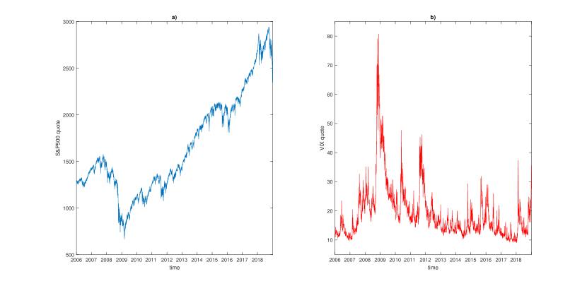
Figure 1: Panel a): 1-minute S&P500 trade prices over the period 2006-2018; panel b): Opening quotes of the VIX index over the period 2006-2018.

3.1 Spot variance estimation

The latent spot variance at the beginning of each trading day is reconstructed from $1$-minute prices using the Fourier methodology, according to Malliavin and Mancino (2009) and Cuchiero and Teichmann (2015). More precisely, we first detect the presence of jumps in our sample data and, secondly, we use the the estimator by Cuchiero and Teichmann (2015), with sparse sampling, in days where jumps are detected. In the other days, the estimator by Malliavin and Mancino (2009) is employed with the entire high frequency data set. For the reader convenience, we briefly recall the definition and main properties of these spot volatility estimators.

The Fourier estimator by Malliavin and Mancino (2009) is defined as follows. Let $[0,2\pi]$ be the time horizon and consider the time grid $\{0=t_{0}<\ldots<t_{m}=2\pi\}$. For any integer $k$, $|k|\leq 2N$, define the discrete Fourier transform

$$c_{k}({\rm d}X_{m}):={1\over{2\pi}}\sum_{j=1}^{m}e^{-{\rm i}kt_{j-1}}(X_{t_{j}}-X_{t_{j-1}}).$$ (16)

Then, for any integer $k$, $|k|\leq N$, consider the following convolution formula

$$c_{k}(V^{m}_{N}):={2\pi\over{2N+1}}\sum_{|h|\leq N}c_{h}({\rm d}X_{m})c_{k-h}({\rm d}X_{m}).$$ (17)

Formula (17) contains the identity relating the Fourier transform of the log-price process $X_{t}$ to the Fourier transform of the variance $V_{t}$. By (17) we gather all the Fourier coefficients of the variance function by means of the Fourier transform of the log-returns. Then, the reconstruction of the variance function $V_{t}$ from its Fourier coefficients is obtained through the Fourier-Fejér summation, i.e., the Fourier estimator of the spot variance is defined as follows: for any $t\in(0,2\pi)$,

$$\widehat{V}^{m}_{N,M}(t)=\sum_{|k|<M}\left(1-{|k|\over M}\right)c_{k}(V^{m}_{N})\ {\rm e}^{{\rm i}kt}.$$ (18)

We note that the definition of the estimator $\widehat{V}^{m}_{N,M}(t)$ depends on three parameters, the number of data $m$ and the two cutting frequencies $N,M$. An appropriate choice of the cutting frequencies is needed to filter out the microstructure noise effects. In fact, on one side the estimation of the instantaneous volatility benefits from the availability of a large amount of data, at least from a statistical point of view. On the other side, high-frequency data are affected by microstructure noise effects deriving from, e.g., bid-ask bounces, infrequent trading and price discreteness. Therefore, it is necessary to employ volatility estimators which are able to filter out microstructure noise contaminations. The estimator of the spot variance $V_{t}$ by means of the Fourier method has been designed to this aim, and is robust to the presence of different types of noise contaminations in the price process, see Mancino and Sanfelici (2008).

The Fourier method to estimate the spot variance has been extended to the case where jumps are present in the price process by Cuchiero and Teichmann (2015). The procedure has two steps. First, an estimate of the Fourier coefficients of a continuous invertible function $\varrho(V)$ of the instantaneous variance is obtained. The estimator of the $k$-th Fourier coefficient takes the form

$$\sum_{j=1}^{m}{1\over m}\,{\rm e}^{-{\rm i}kt_{j-1}}g(\sqrt{m}(X_{t_{j}}-X_{t_{j-1}})),$$ (19)

where the function $g$ can assume different specifications. We will consider $\varrho_{g}(V_{t})={\rm e}^{-{V_{t}/2}}$, that is we choose here $g(x)={\rm cos}\ x$. Second, we invoke the Fourier-Fejér inversion formula as in (18) to reconstruct the path of the process $\varrho(V)$ as follows:

$$\frac{1}{2\pi}\sum_{j=1}^{m}\frac{1}{m}F_{M}(t-t_{j-1})\ g(\sqrt{m}(X_{t_{j}}-X_{t_{j-1}})),$$ (20)

where $F_{M}(x)$ is the Fejér kernel. Note that also (18) can be re-written by means of $F_{M}(x)$, see Mancino and Recchioni (2015). Finally, this is translated into an estimator of the spot variance by inverting the function $\varrho(\cdot)$. The obtained estimator of the instantaneous variance is consistent and asymptotically efficient in the absence of microstructure noise.

In order to assess whether the characteristics of the S&P500 $1$-minute prices data require either the use of the jump-robust Fourier estimator of spot volatility or not, we perform the following tests. First, we split the sample into daily subsamples and apply the test by Aït-Sahalia and Xiu (2019) for the null hypothesis that the price is an Itô semimartingale. Test results at the $95\%$ confidence level, illustrated in the Figure 2, panel a), show, consistently with the literature Andersen et al. (2001), that the impact of microstructure noise on prices can be considered negligible at the $5$-minute frequency. This finding is consistent with the behavior of the volatility signature (Figure 2, panel b)), which shows that the total Realized Variance of the sample stabilizes, around $0.4$, from the $5$-minute frequency and downwards.

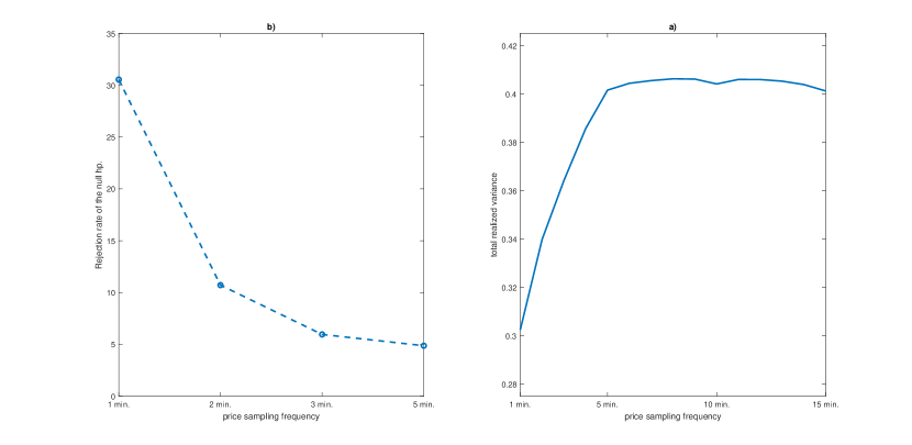
Figure 2: Panel a): rejection rate of the null hypothesis of the noise-detection test by Aït-Sahalia and Xiu (2019), performed on daily subsamples of S&P500 prices over the period 2006-2018, for different sampling frequencies; panel b): volatility signature plot, i.e., total S&P500 realized variance for the period 2006-2018 as a function of the price sampling frequency.

Secondly, after downsampling the log-price series at the $5$-minute frequency, we apply the jump detection test by Corsi et al. (2010) for the null hypothesis that the price is a continuous semimartingale. Test results at the $99.9\%$ confidence level show that jumps are detected in $10.35\%$ of the daily subsamples over the period 2006-2018. Figure 3 shows the values of the test statistic computed from daily subsamples (panel a)) and the ensuing percentage of days with jumps per year (panel b)). The percentage of jumps detected per year is compatible with the empirical results in Corsi et al. (2010).

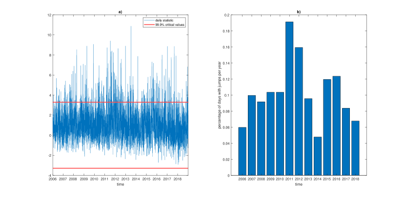
Figure 3: Panel a): values of the statistic of the jump-detection test by Corsi et al. (2010) computed over the period 2006-2018; panel b): ensuing percentage of days with jumps per year.

Based on the results of the two tests, in order to obtain spot variance estimates, we proceed as follows. On the consecutive days in which the hypothesis of absence of jumps is not rejected (amounting approximately to $90\%$ of the sample), the Fourier estimator (18) is applied with all prices recorded at $1$-minute frequency. Instead, for the sparse days in which jumps are detected (amounting approximately $10\%$ of the sample) we use spot variance estimates obtain through the Fourier estimator (20), applied to sparsely sampled 5-minute prices. In the case of the estimator (18), the cutting frequencies have been selected as $N=m^{2/3}/2$ and $M=m^{2/3}/(16\pi)$, according to Mancino and Recchioni (2015), who find these cutting frequencies to be optimal in the presence of different types of noise and noise intensities. For the estimator (20), instead, the frequency $M$ is selected as $M=(m/4)^{2/3}$, in accordance to Cuchiero and Teichmann (2015). The resulting spot variance estimates at the beginning of each trading day are shown in Figure 4.

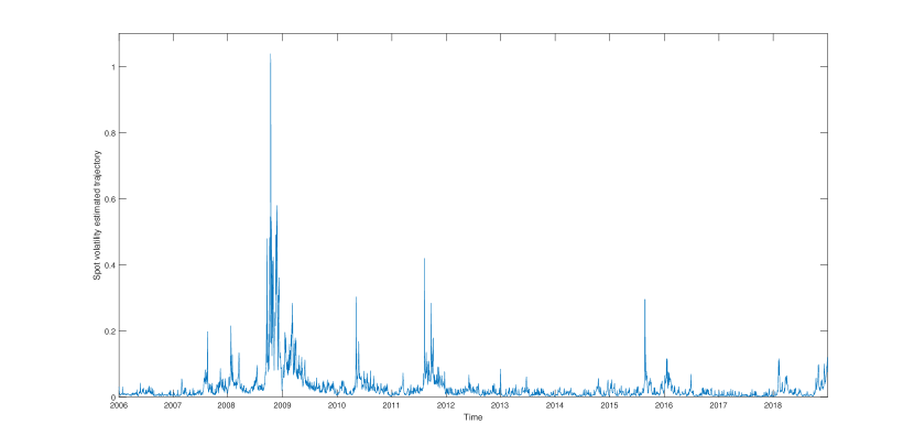
Figure 4: Estimated S&P500 spot variance trajectory on a daily grid over the period 2006-2018.

3.2 Empirical test results

We now focus on testing the empirical link between the rate of the variance swap with time to maturity equal to one month, i.e., the VIX index squared, and the couple spot variance - log return. If estimates of the unobservable spot variance are available, equation (15) can be rewritten, in the case of the S&P500 index, as follows. Let $L=3267$ denote the number of days in our sample and let $\tau=1/12$. Then, for $t_{i}=\frac{i-1}{252}$, $i=1,2,...,L$, we write

$${\rm VIX}^{2}_{t_{i}}=p_{0,0}(\tau)+p_{1,0}(\tau)\,X_{t_{i}}+p_{0,1}(\tau)\,\widehat{V}^{m}_{{t_{i}}}+p_{2,0}(\tau)\,X^{2}_{t_{i}}+p_{1,1}(\tau)\,X_{t_{i}}\,\widehat{V}^{m}_{{t_{i}}}+p_{0,2}(\tau)\,(\widehat{V}^{m}_{{t_{i}}})^{2},$$ (21)

where:

• ${\rm VIX}_{t_{i}}$ denotes the opening quote of the VIX index on $i$-th day;

• $X_{t_{i}}$ denotes the opening log-price of the S&P500 index on $i$-th day;

• $\widehat{V}^{m}_{{t_{i}}}$ denotes the estimated spot variance at the beginning of the $i$-th day, obtained from a sample of size $m$ using the estimator (18) or (20).

Some comments are needed. First, based on the results of Propositions 2.2 and 2.5, the presence of jumps does not spoil the affine/polynomial structure, thus the regression coefficients $p_{i,j}(\tau),\ i,j=0,1,2$, include the potential contribution of jumps. In the following, we drop the argument $\tau$ from $p_{i,j}(\tau)$ as we always consider monthly coefficients. Secondly, the consistency of the spot variance estimators (18) and (20) allows us to neglect the finite-sample error related to estimation of $V^{m}_{t_{i}}$.

We aim at testing the significance of the estimates of the coefficients in equation (21) within three progressively broader frameworks: the affine framework, introduced in Definition 2 and extended in Definition 3 (hereafter, affine framework); the polynomial framework of Definition 4, where the variance swap rate is first assumed to be a quadratic function of $V$ only (hereafter, quadratic framework) and then is assumed to be a polynomial function of the couple $(X,V)$ (hereafter, polynomial framework).

3.2.1 Affine framework

In this paragraph we consider the exponentially affine and exponentially mean-reverting variance models, which both imply the existence of an affine relationship between the variance swap rate and the spot variance. Note that in the affine framework the equation (21) reduces to

$${\rm VIX}_{t_{i}}^{2}=p_{0,0}+p_{0,1}\,\widehat{V}^{m}_{{t_{i}}}.$$ (22)

Recall that the main discriminant factor between the exponentially affine model and its extension to the exponentially mean-reverting variance class is that the former implies the coefficients $p_{0,0}$ and $p_{0,1}$ in equation (22) are strictly positive. Thus, we are not only interested in testing if the affine dependence between the variance swap rate and the spot variance is satisfied by empirical data, but also in verifying if both parameter estimates are significantly different from zero, as this would allow us to accept or reject the exponentially affine framework.

The coefficients in (22) are estimated using OLS. Note that ${\rm VIX}^{2}_{t_{i}}$ is scaled as $({{\rm VIX}_{t_{i}}}/{100})^{2}/({30}/{365})$, in order to obtain properly normalized coefficient estimates. In order to avoid performing a spurious regression (see Granger and Newbold (1974)), we first test for the null hypothesis of the presence of a unit root in the VIX squared series and in the spot volatility estimates series, using the Augmented Dickey-Fuller test (see Dickey and Fuller (1979)). For both series, test results at the $99\%$ confidence level reject the null hypothesis. Thus, the two series are assumed to be stationary in the rest of the analysis. The results of the OLS estimation are overwhelming: we obtain an $R^{2}$ larger than $0.95$ and significant coefficients estimates, as shown in Table 1. In particular, the fact that both coefficient estimates are significant and positive suggests that an exponentially affine framework is a suitable fit for the S&P500 data over the period 2006-2018. Note that the regression standard errors have been computed using the Newey-West methodology (see Newey and West (1987)), to account for the presence of heteroskedasticity and autocorrelations in the residuals.

Table 1: Affine framework (22): estimation from S&P500 data over the period 2006-2018
(p-values less than $10^{-4}$ are reported as zero).

framework	coeff.	estimate	std. err.	t stat.	p value	${R}^{2}$
affine	$p_{0,0}$	0.0011	0.0003	4.1312	0	0.9582
	$p_{0,1}$	0.0801	0.0106	7.5512	0

A natural question that arises is whether the coefficients in (22) are sensitive to events of distress, such as the global financial crisis of 2008, or are stable over time, instead. To investigate this aspect, the coefficients of (22) are estimated on yearly subsamples. Estimation results are detailed in Table 2 and offer interesting insights.

Table 2: Affine framework (22): estimation from S&P500 data over yearly subsamples
(p-values less than $10^{-4}$ are reported as zero).

Affine framework
year	coeff.	estimate	std. err.	t stat.	p value	${R}^{2}$
2006	$p_{0,0}$	0.0009	0.0001	10.5224	0	0.4405
	$p_{0,1}$	0.0394	0.0144	2.7279	0.0064
2007	$p_{0,0}$	0.0012	0.0003	3.6437	0.0003	0.6587
	$p_{0,1}$	0.0714	0.0171	4.1778	0
2008	$p_{0,0}$	0.0017	0.0013	1.3576	0.1746	0.9795
	$p_{0,1}$	0.0776	0.0147	5.2930	0
2009	$p_{0,0}$	0.0026	0.0007	3.8468	0.0001	0.8630
	$p_{0,1}$	0.1095	0.0134	8.1877	0
2010	$p_{0,0}$	0.0021	0.0007	3.1524	0.0016	0.8235
	$p_{0,1}$	0.0779	0.0261	2.9862	0.0028
2011	$p_{0,0}$	0.0012	0.0011	1.0170	0.3092	0.9110
	$p_{0,1}$	0.1194	0.0344	3.4696	0.0005
2012	$p_{0,0}$	0.0019	0.0002	12.4158	0	0.3193
	$p_{0,1}$	0.0458	0.0103	4.4609	0
2013	$p_{0,0}$	0.0013	0.0001	17.2232	0	0.4952
	$p_{0,1}$	0.0292	0.0069	4.2261	0
2014	$p_{0,0}$	0.0012	0.0001	8.0686	0	0.5410
	$p_{0,1}$	0.0405	0.0179	2.2641	0.0236
2015	$p_{0,0}$	0.0012	0.0005	2.4669	0.0136	0.8869
	$p_{0,1}$	0.0579	0.0276	2.0938	0.0363
2016	$p_{0,0}$	0.0012	0.0001	15.9943	0	0.8168
	$p_{0,1}$	0.0499	0.0048	10.3033	0
2017	$p_{0,0}$	0.0009	0.0001	21.6109	0	0.2484
	$p_{0,1}$	0.0204	0.0050	4.0758	0
2018	$p_{0,0}$	0.0010	0.0001	10.0552	0	0.9122
	$p_{0,1}$	0.0627	0.0051	12.1783	0

In periods of distress, like 2008, when the global financial crisis broke out, or 2011, when the financial turmoil related to sovereign debt crisis in the Euro area took place, the intercept estimates are not significant at the 95% confidence level. Thus, based on Proposition 2.3, S&P500 data in 2008 and 2011 look consistent only with the broader assumption of an exponentially mean-reverting variance data-generating process, which poses no restrictions on the sign of the coefficients. In other words, results on yearly subsamples tilt the balance in favor of the use, during crisis periods, of models that imply a linear relationship between the variance swap rate and the spot variance, such as the model by Hull and White (1987) and the rough-Bergomi by Bayer et al. (2016); Jacquier et al. (2018) model (see the discussion in Section 2.2). Finally, note that the empirical analysis suggests that the drift of the variance process is affine in the variance itself. As a consequence, models with stronger mean reversion, e.g., the $3/2$ model, are not coherent with our empirical findings.

3.2.2 Quadratic framework

In this paragraph we extend the analysis to take into account a possible quadratic link between variance swap rates and spot variance. Through this section, the term quadratic is used to refer to polynomial models that are not exponentially affine, where no risk of confusion exists. According to Propositions 2.5 and 2.6, when polynomial models with jumps are considered and/or discrete-sampling effects can not be neglected, the variance swap rate is a bivariate polynomial in $X$ and $V$. Based on these results, the rest of our empirical study is aimed to investigating the possible existence of a quadratic link between the variance swap rate and the spot variance and/or the log-price. In particular, the analysis is split into two parts. In this paragraph, devoted to what we have called the quadratic framework, we check if a quadratic form with respect to the spot variance fits the data better than an affine form. In the next paragraph we will deal with the general form as in (21). In the quadratic framework, equation (21) reads

$${\rm VIX}^{2}_{t_{i}}=p_{0,0}+p_{0,1}\,\widehat{V}^{m}_{{t_{i}}}+p_{0,2}\,\left(\widehat{V}^{m}_{{t_{i}}}\right)^{2}.$$ (23)

However, we measure the sample linear correlation between spot variance estimates and their square and find it to be approximately equal to $0.84$, thus signalling the presence of collinearity, which represents a violation of the OLS hypotheses. The problem of collinearity is typical of polynomial regressions and can be solved by transforming the regressors in equation (23) through the use of orthogonal polynomials, i.e., by performing an orthogonal polynomial regression (see Narula (1979)). This way we are able to isolate the actual additional contribution of the square of variance estimates to the dynamics of the VIX index squared, if any. Accordingly, using the Gram-Schmidt algorithm, we transform the vector of spot variance estimates and the vector of their squared values into orthogonal vectors and estimate the following regression model:

$${\rm VIX}^{2}_{t}=q_{0,0}+q_{0,1}\;Z^{(1)}_{t}+q_{0,2}\;Z^{(2)}_{t},$$ (24)

where $Z^{(1)}$ and $Z^{(2)}$ denote, respectively, the orthogonal transformations of the vector of the spot variance estimates and the vector of the squared spot variance estimates. Clearly, the coefficients in equation (24) are not comparable to those those in (23). However, this is not relevant for our study, as we aim only at assessing the significance of the additional contribution of the squared variance estimates to the dynamics of the VIX squared, not at making inference of the coefficients in equation (23).

The results of the OLS estimation of the coefficients in (24) over the period 2006-2018 are reported in Table 3. These results point out that the additional contribution of the squared spot variance is not statistically significant. In order to interpret these results, we first need to recall that, from one side the class of polynomial models includes exponentially affine one as a subclass, from the other, in the presence of jumps, while the polynomial model gives rise to a quadratic correction (see Proposition 2.5), the exponentially affine model still ensures an affine link between the variance swap rate and the spot variance. Therefore, as in Paragraph 3.2.1, we have already ascertained that the exponentially affine framework is a suitable fit for S&P500 data over the period 2006-2018, we deduce that the results in Table 3 confirm the adequacy of the exponentially affine framework in capturing the empirical features of S&P500 data. In other words, Table 3 points towards the fact that the extension to the quadratic framework is not necessary to capture the empirical link between the variance swap rate and the spot variance.

Furthermore, Table 3 offers additional interesting insight. Recall that the computation of the VIX index is based on a daily sampling scheme. Thus, it is natural to ask whether the VIX index squared is adequately approximated by its asymptotic counterpart, namely the future expected quadratic variation. If this were not the case, one would observe a significant quadratic correction due to the discrete sampling, see Proposition 2.6. As this is not the case, we infer that the continuous limit represents a very good approximation, thus providing empirical support to the numerical result by Broadie and Jain (2008).

Table 3: Quadratic framework (24): estimation from S&P500 data over the period 2006-2018
(p-values less than $10^{-4}$ are reported as zero).

framework	coeff.	estimate	std. err.	t stat.	p value	$R^{2}$
quadratic	$q_{0,0}$	0.0033	0.0001	27.1498	0	0.9585
	$q_{0,1}$	0.2464	0.0328	7.5065	0
	$q_{0,2}$	0.0016	0.0471	0.0339	0.9730

As in the affine framework (see Paragraph 3.2.1), we also analyze yearly sub-samples in order to evaluate if coefficient estimates are sensitive to events of distress. The ensuing estimation results are shown in Table 4.

Table 4: Quadratic framework (24): estimation from S&P500 data over yearly subsamples
(p-values less than $10^{-4}$ are reported as zero).

Quadratic framework
year	coeff.	estimate	std. err.	t stat.	p value	$R^{2}$
2006	$q_{0,0}$	0.0017	0.0007	2.4286	0.0152	0.4482
	$q_{0,1}$	0.6899	0.3807	2.4578	0.0140
	$q_{0,2}$	-0.5633	0.5811	-0.9694	0.3323
2007	$q_{0,0}$	0.0023	0.0001	19.2127	0	0.6695
	$q_{0,1}$	0.2461	0.0486	5.0580	0
	$q_{0,2}$	-0.3650	0.0543	-6.7178	0
2008	$q_{0,0}$	0.0043	0.0030	1.4330	0.1518	0.9799
	$q_{0,1}$	0.2366	0.0290	8.1595	0
	$q_{0,2}$	0.0602	0.1030	0.5846	0.5588
2009	$q_{0,0}$	0.0047	0.0002	20.4214	0	0.8720
	$q_{0,1}$	0.1540	0.0510	3.0196	0.0025
	$q_{0,2}$	-0.3213	0.0665	-4.8310	0
2010	$q_{0,0}$	0.0037	0.0001	30.3236	0	0.8377
	$q_{0,1}$	0.0257	0.0118	2.1780	0.0294
	$q_{0,2}$	-0.1861	0.0560	-3.3243	0.0009
2011	$q_{0,0}$	0.0037	0.0030	1.2330	0.2175	0.9298
	$q_{0,1}$	0.0426	0.0164	2.5976	0.0094
	$q_{0,2}$	-0.3284	0.1004	-3.2707	0.0011
2012	$q_{0,0}$	0.0032	0.0008	3.7571	0	0.3196
	$q_{0,1}$	0.1534	0.0337	4.5479	0
	$q_{0,2}$	0.0099	0.2435	0.0407	0.9676
2013	$q_{0,0}$	0.0011	0.0003	3.7472	0.0002	0.4961
	$q_{0,1}$	0.3715	0.1235	2.1682	0.0026
	$q_{0,2}$	-0.3151	0.0872	-3.6135	0
2014	$q_{0,0}$	0.0053	0.0014	3.2852	0.0002	0.7387
	$q_{0,1}$	1.2842	0.5923	2.0560	0.0301
	$q_{0,2}$	0.7698	0.4071	1.8909	0.0586
2015	$q_{0,0}$	0.0025	0.0001	23.5592	0	0.8896
	$q_{0,1}$	0.0283	0.0035	8.0547	0
	$q_{0,2}$	-0.0919	0.0195	-4.7018	0
2016	$q_{0,0}$	0.0023	0.0001	16.8683	0	0.8668
	$q_{0,1}$	0.1083	0.0407	2.6609	0.0078
	$q_{0,2}$	-0.2189	0.0865	-2.5289	0.0114
2017	$q_{0,0}$	0.0054	0.0018	3.0369	0.0024	0.3295
	$q_{0,1}$	2.7480	0.7214	3.8095	0.0001
	$q_{0,2}$	-1.8918	0.4822	-3.9233	0.0001
2018	$q_{0,0}$	0.0029	0.0003	10.0292	0	0.9140
	$q_{0,1}$	0.2417	0.1191	2.0294	0.0424
	$q_{0,2}$	0.0377	0.1037	0.3636	0.7162

Note that the quadratic term is not statistically significant in 2006, 2008, 2012, 2014 and 2018. Based on Figure 1, panel b), and the detailed analysis in Horst and Xu (2019), these years appear truly different, in terms of the state of the financial market. For instance, during 2008 and 2018, the VIX exhibits spikes, related, respectively, to the global financial crisis and the ‘China-US trade war’. In contrast, 2006 and 2012 do not experience relevant economic events, see Horst and Xu (2019). The year 2014 represents an intermediate situation, where the VIX is almost flat until the end of October, when a cluster of spikes arises due to the end of quantitative easing policy by the Federal Reserve in the US. Thus, it is hard to attribute the statistical significance of the quadratic terms in Table 4 to events of financial distress.

Focusing on the frequency of price jumps in Figure 3, panel b), we highlight that 2006, 2014, and 2018 show a relatively low percentage of days with jumps. Thus, keeping in mind the result in Proposition 2.5, the non-significance of the quadratic coefficient in these years could be linked to the low percentage of days with jumps. The number of jumps in 2012 seems not coherent with this interpretation of the results in Table 4. Indeed, the quadratic term is not statistically significant in 2012, despite the fact that the percentage of days with jumps in 2012 is the second largest after 2011. However, 2012 can be deemed as an atypical year, in terms of market liquidity. In 2012 a series of important expansionary monetary policies were started by central banks to respond to the Euro-zone debt crisis and its international ramifications. These include the decision by the European Central Bank to cut its rates in multiple steps and to start a long-term refinancing operation (LTRO) during the first trimester of 2012, and the decision by the US Federal Open Market Committee to start a quantitative easing in September and to increase it in December of 2012. Thus, the year 2012 is characterized by an atypical number of positive jumps in response to this new paradigm of ‘Infinity Quantitative Easing’, that massively increased the market liquidity.

3.2.3 Polynomial framework

In the last paragraph, the polynomial framework (21) is analyzed. Before fitting this model, we examine the sample correlation matrix of the regressors, which is shown in Table 5.

Table 5: Sample correlation matrix of the regressors of the polynomial form (21) over the period 2006-2018.

	$\widehat{V}_{t}$	$\widehat{V}^{2}_{t}$	$X_{t}$	$X^{2}_{t}$	$X_{t}\widehat{V}_{t}$
$\widehat{V}_{t}$	1
$\widehat{V}^{2}_{t}$	0.8394	1
$X_{t}$	-0.3702	-0.1814	1
$X^{2}_{t}$	-0.3615	-0.1765	0.9997	1
$X_{t}\widehat{V}_{t}$	0.9992	0.8341	-0.3550	-0.3465	1

This table provides empirical evidence of the existence of an almost perfect linear dependence between the log-price and its square, and between the spot variance and the product of the log-price and the spot variance. Moreover, the analysis conducted in Section 3.2.2 has already shown that the additional contribution of the squared spot variance estimates to the dynamics of the squared VIX is not significant. Thus, it remains only to evaluate the additional contribution of the log-price. This polynomial framework could then be associated with a fully affine form in both the log-return and the spot variance.

In this regard, recall that it is a well-known stylized fact that asset price series are non-stationary. Indeed, the Augmented Dickey Fuller test, performed at the 90% confidence level, confirms that our log-price series has a unit root. To cope with the non-stationarity of the log-price series, we estimate the coefficients in equation (23) after replacing log-prices with their detrended values, i.e., their values minus their sample mean. The estimation results are summarized in Table 6.

Table 6: Polynomial (fully affine) framework: estimation from S&P500 data over the period 2006-2018
(p-values less than $10^{-4}$ are reported as zero; $p_{1,0}$ indicates the coefficient of the detrended price).

framework	coeff.	estimate	std. err.	t stat.	p value	${R}^{2}$
polynomial	$p_{0,0}$	0.0013	0.0003	4.9275	0	0.9592
(fully affine)	$p_{0,1}$	0.0725	0.0106	6.8284	0
	$p_{1,0}$	-0.0015	0.0009	-1.7653	0.0775

Based on Table 6, the contribution of the log-price is not statistically significant at the $95\%$ confidence level, but only at $90\%$ level. Overall, this result confirms that the affine framework is sufficient to adequately fit for our sample.

Finally, it is worth evaluating if the additional contribution of the price in explaining the dynamics of the VIX index squared is statistically significant on yearly subsamples, i.e., under different economic scenarios. The results of the year-by-year estimation are summarized in Table 7 and are in line with the whole-sample results.

Table 7: Polynomial (fully affine) framework: estimation from S&P500 data over yearly subsamples
(p-values less than $10^{-4}$ are reported as zero; $p_{1,0}$ indicates the coefficient of the detrended price).

Polynomial (fully affine) framework
year	coeff.	estimate	std. err.	t stat.	p value	${R}^{2}$
2006	$p_{0,0}$	0.0009	0.0004	2.2500	0.0244	0.6012
	$p_{0,1}$	0.0240	0.0105	2.2850	0.0223
	$p_{1,0}$	-0.0043	0.0019	-2.3374	0.0194
2007	$p_{0,0}$	0.0016	0.0004	4.1944	0.0000	0.6699
	$p_{0,1}$	0.0712	0.0163	4.3566	0.0000
	$p_{1,0}$	0.0054	0.0031	1.7258	0.0844
2008	$p_{0,0}$	0.0019	0.0011	1.7273	0.0841	0.9796
	$p_{0,1}$	0.0501	0.0159	3.1520	0.0016
	$p_{1,0}$	-0.0322	0.0084	-3.8116	0.0001
2009	$p_{0,0}$	0.0038	0.0013	2.8957	0.0038	0.9093
	$p_{0,1}$	0.0728	0.0188	3.8755	0.0001
	$p_{1,0}$	-0.0164	0.0041	-3.9743	0.0001
2010	$p_{0,0}$	0.0020	0.0007	2.8571	0.0043	0.8291
	$p_{0,1}$	0.0428	0.0149	2.8654	0.0042
	$p_{1,0}$	-0.0150	0.0043	-3.5235	0.0004
2011	$p_{0,0}$	0.0056	0.0033	1.6970	0.0897	0.9338
	$p_{0,1}$	0.0567	0.0251	2.2543	0.0242
	$p_{1,0}$	-0.0402	0.0111	-3.6063	0.0003
2012	$p_{0,0}$	0.0014	0.0005	2.8000	0.0051	0.3944
	$p_{0,1}$	0.0216	0.0068	3.1747	0.0015
	$p_{1,0}$	0.0003	0.0003	0.8642	0.3875
2013	$p_{0,0}$	0.0013	0.0001	17.5755	0	0.4959
	$p_{0,1}$	0.0296	0.0068	4.3350	0
	$p_{1,0}$	0.0003	0.0004	0.7629	0.4455
2014	$p_{0,0}$	0.0014	0.0004	3.2852	0.0010	0.5516
	$p_{0,1}$	0.0384	0.0187	2.0560	0.0398
	$p_{1,0}$	-0.0012	0.0020	-0.5993	0.5490
2015	$p_{0,0}$	0.0101	0.0016	6.3290	0	0.8942
	$p_{0,1}$	0.0117	0.0030	3.8894	0.0001
	$p_{1,0}$	-0.0305	0.0057	-5.3606	0
2016	$p_{0,0}$	0.0040	0.0008	4.7158	0	0.8996
	$p_{0,1}$	0.0350	0.0040	8.7464	0
	$p_{1,0}$	-0.0088	0.0027	-3.2395	0.0012
2017	$p_{0,0}$	0.0018	0.0003	6.2120	0	0.4695
	$p_{0,1}$	0.0155	0.0048	3.2280	0.0012
	$p_{1,0}$	-0.0021	0.0006	-3.5198	0.0004
2018	$p_{0,0}$	0.0054	0.0021	2.5861	0.0097	0.9133
	$p_{0,1}$	0.0489	0.0074	6.6009	0
	$p_{1,0}$	-0.0075	0.0036	-2.1090	0.0349

Remark 1.

The study of Section 3.2 can be performed also using alternative spot variance estimators to reconstruct the series $\widehat{V}^{m}_{t_{i}}$. In fact, we have replicated the empirical study using the localized version of the two-scale realized variance and bipower variation (see Chapter 8 in Aït-Sahalia and Jacod (2014)), in place, respectively, of the Fourier estimator by Malliavin and Mancino (2009) and the Fourier estimator by Cuchiero and Teichmann (2015). The corresponding results are perfectly in line with those in Tables $1-7$, both in terms of the significance of the coefficient estimates and the $R^{2}$ values.

4 Conclusions

This paper provides empirical evidence that S&P500 data over the period 2006-2018 are coherent with the exponentially affine framework, introduced by Kallsen et al. (2011), who analytically prove the existence of an affine relationship between the expected future variance, i.e., the variance swap rate, and the spot variance. This paper collects empirical evidence that this affine relationship fits the data overwhelmingly well, with statistically significant coefficients and an $R^{2}$ larger than $0.95$. Further, this paper provides empirical evidence that the daily sampling used to compute the actual variance swap rates is frequent enough to erase the quadratic correction due to discrete sampling. The quadratic correction is expected within the polynomial framework, which includes the exponentially affine framework as a special case. This empirical non-parametric result confirms the result by Broadie and Jain (2008), which was obtained on data simulated from four parametric models belonging to the exponentially affine class.

The paper focuses also on yearly subsamples, in order to evaluate the sensitivity to events of financial distress. Empirical results on yearly subsamples are more nuanced. In particular, it emerges that the exponentially affine framework could be rejected in 2008 and 2011. These two years include the outbreaks of two global financial crisis sparked, respectively, by the American housing market and the sovereign debt in the Euro area. Models in the exponentially mean-reverting variance framework seem more adequate to capture the features of empirical data in those two years of financial distress. Finally, the significance of the quadratic coefficients in years with a relatively large number of price jumps supports the use of polynomial models in the presence of more frequent jumps.

Funding

S.Scotti acknowledges financial support from the Institut Europlace de Finance grant ‘Clusters and Information Flow: Modelling, Analysis and Implications’ and from a visiting grant received by the University of Florence.
Part of the research was completed while M.E.Mancino was visiting the Université de Paris under a visiting funding scheme, which the author acknowledges.

5 Proofs

Proof.

(of Proposition 2.3)

Here we adopt, where no ambiguity arises, the parameter notation introduced in Lemma 4.2 of Kallsen et al. (2011) for the exponentially affine model. Using the equation for $\Psi^{V}_{u}$ and $\Phi^{V}_{u}$ in Proposition 2.2 and differentiating the two equations with respect to $u$, we have

$$\frac{\upartial^{2}\Psi^{V}_{u}}{\upartial u\upartial t}(t) = \gamma_{1}^{11}\Psi^{V}_{u}(t)\frac{\upartial\Psi^{V}_{u}(t)}{\upartial u}+\beta_{1}^{1}\frac{\upartial\Psi^{V}_{u}(t)}{\upartial u}+\gamma_{1}^{22}$$

$$+\int_{\mathbb{R}^{+}\times\mathbb{R}}\left(e^{x_{1}\Psi^{V}_{u}(t)+ux_{2}^{2}}\left(x_{1}\frac{\upartial\Psi^{V}_{u}(t)}{\upartial u}+x_{2}^{2}\right)-\frac{\upartial\Psi^{V}_{u}(t)}{\upartial u}h(x_{1})\right)\kappa_{1}({\rm d}x),$$

$$\frac{\upartial\Phi^{V}_{u}(t)}{\upartial u} = \int_{0}^{t}\left[\beta_{0}^{1}\frac{\upartial\Psi^{V}_{u}(s)}{\upartial u}+\gamma_{0}^{22}+\int_{\mathbb{R}^{+}\times\mathbb{R}}\left(e^{x_{1}\Psi^{V}_{u}(s)+ux_{2}^{2}}\left(x_{1}\frac{\upartial\Psi^{V}_{u}(s)}{\upartial u}+x_{2}^{2}\right)-\frac{\upartial\Psi^{V}_{u}(s)}{\upartial u}h(x_{1})\right)\kappa_{0}({\rm d}x)\right]{\rm d}s\,.$$

Taking $u=0$ and recalling that $\Psi^{V}_{0}(t)=0$ for all $t$, we obtain the relations satisfied by $(\Psi,\Phi)$, that read

$$\frac{\upartial\Psi}{\upartial t}(t) = \beta_{1}^{1}\Psi(t)+\gamma_{1}^{22}+\int_{\mathbb{R}^{+}\times\mathbb{R}}\left(x_{1}\Psi(t)+x_{2}^{2}-\Psi(t)h(x_{1})\right)\kappa_{1}({\rm d}x),$$

$$\Phi(t) = \int_{0}^{t}\left[\beta_{0}^{1}\Psi(s)+\gamma_{0}^{22}+\int_{\mathbb{R}^{+}\times\mathbb{R}}\left(x_{1}\Psi(s)+x_{2}^{2}-\Psi(s)h(x_{1})\right)\kappa_{0}({\rm d}x)\right]{\rm d}s\,.$$

Note that in our case $\gamma_{0}^{22}=0$, see (8). Then, splitting the integrals and recalling that $h(x)$ is a truncating function, there exists non-negative parameters $(\widetilde{\beta}_{1}^{1},\widetilde{\beta}_{0}^{1})$, that is the parameters associated with the truncating function $h(x)=x$, such that:

$$\frac{\upartial\Psi}{\upartial t}(t) = \widetilde{\beta}_{1}^{1}\Psi(t)+\gamma_{1}^{22}+\int_{\mathbb{R}^{+}\times\mathbb{R}}x_{2}^{2}\;\kappa_{1}({\rm d}x),$$

$$\Phi(t) = \int_{0}^{t}\left[\widetilde{\beta}_{0}^{1}\Psi(s)+\int_{\mathbb{R}^{+}\times\mathbb{R}}x_{2}^{2}\;\kappa_{0}({\rm d}x)\right]{\rm d}s\,.$$

Note that $\Psi$ solves a non-homogeneous linear differential equation with non-negative external term $\gamma_{1}^{22}+\int_{\mathbb{R}^{+}\times\mathbb{R}}x_{2}^{2}\;\kappa_{1}({\rm d}x)$. This term is zero if and only if $\gamma_{1}^{22}=0$ and $\kappa_{1}({\rm d}x)=0$, that is in the case of the exponential Levy model. We deduce that $\Psi(s)>0$ for all positive $s$, except for the exponential Levy model, for which volatility is constant and thus the stationary distribution is degenerate. We now turn to $\Phi$ and assume $\Psi(s)>0$. Using the integral representation of $\Phi$, we easily obtain that $\Phi>0$ if and only if $\widetilde{\beta}_{0}^{1}\neq 0$ or $\kappa_{0}({\rm d}x)\neq 0$, see also Filipovic (2001). This is equivalent to assuming that the process $V$ is a continuous-state branching process with immigration. Instead, in the case $\widetilde{\beta}_{0}^{1}=0$ and $\kappa_{0}({\rm d}x)=0$, the process $V$ is a continuous-state branching process without immigration. Without immigration continuous-state branching processes do not have a stationary distribution, see Theorem 3.20 and Corollary 3.21 in Li (2011). ∎

Proof.

(of Proposition 2.4)

The quadratic variation of $X$ is rewritten as $[X]_{t}=[X^{c}]_{t}+\sum_{s\leq t}(\Delta X_{s})^{2}$, where $X^{c}$ denotes the continuous part of the log-price $X$. According to (12), we have $[X^{c}]_{t}=\int_{0}^{t}V_{s}{\rm d}s$. It is easy to show that the variance process $V$ is integrable using Gronwall’s lemma, since the drift of the variance process is affine and $Z$ is integrable by hypothesis. We now focus on the jump contribution, $\sum_{s\leq t}(\Delta X_{s})^{2}=\sum_{s\leq t}(\Delta J_{s})^{2}$. Recalling that the process $J$ is square-integrable, we obtain that the optional version of the quadratic variation $[X]_{t}$ is finite almost surely. Introducing the predictable version $\langle X\rangle_{t}$ of the quadratic variation and recalling that the optional and the predictable version of the quadratic variation differ by a martingale, we obtain that

$${E}\left[[X]_{\tau}\right]={E}\left[\langle X\rangle_{\tau}\right]={E}\left[\int_{0}^{\tau}V_{s}{\rm d}s+\int\int_{0}^{\tau}\zeta^{2}\nu(d\zeta,{\rm d}s)\right]\,.$$

Considering first the jump term, exploiting that $\nu$ is affine in the variance process $V$, we deduce that the jump part is affine in the expectation of the integral of the variance process. Focusing now on the term ${E}\left[\int_{0}^{\tau}V_{s}{\rm d}s\right]$, we consider the integral version of the SDE (12), i.e.

$$V_{t}-V_{0}=\kappa\int_{0}^{t}(\theta-V_{s}){\rm d}s+Z_{t}.$$

Taking the expectation, we obtain that ${E}\left[\int_{0}^{\tau}V_{s}{\rm d}s\right]=\kappa^{-1}\left(\tau\kappa\theta+V_{0}-{E}\left[V_{\tau}\right]\right)$ and ${E}\left[V_{t}\right]$ satisfies a linear ODE. This result, combined with the previous result, proves that the expectation of the quadratic variation is an affine function of the initial spot variance. ∎

Proof.

(of Proposition 2.5)

According to the characterization in Proposition 2.12 of Cuchiero et al. (2012), if $(X,V)$ is a $2$-polynomial process then

$$[X,X]_{t}=\int_{0}^{t}V_{s}{\rm d}s+\int_{0}^{t}\int\zeta^{2}\nu({\rm d}\zeta,{\rm d}s)=:\int_{0}^{t}a(X_{s},V_{s}){\rm d}s,$$

where $a\in{\cal P}_{2}$. Then, the result for $E^{(x,v)}[[X,X]_{t}]$ follows from Theorem 3.2 in Cuchiero (2011) and the application of the stochastic Fubini theorem.

In particular, if we consider the quadratic variation of $X^{c}$, together with the evolution (8), we have that $[X^{c}]_{t}=\int_{0}^{t}V_{s}{\rm d}s$. Taking the expectation and applying the stochastic Fubini theorem, we obtain ${E}\left[[X^{c}]_{t}\right]=\int_{0}^{t}{E}\left[V_{s}\right]{\rm d}s$. Now, using the hypothesis that $(X,V)$ is $2$-polynomial, we see that the function $f(x,v)=v\in{\cal P}_{1}$, and integrating we obtain the result. ∎

Proof.

(of Proposition 2.6)

Using the definition of realized variance $RV^{m}_{[0,\tau]}$ given in (2), we take the expected value of $RV^{m}$. Due to the finiteness of the sum, the expected value of $RV^{m}_{[0,\tau]}$ gives

$${E}^{(x,v)}\left[RV^{m}_{[0,\tau]}\right]=\sum_{k=1}^{m}{E}^{(x,v)}\left[\left(X_{t_{k}}-X_{t_{k-1}}\right)^{2}\right].$$

Noting that the function inside the expectation belongs to ${\cal P}_{2}$, we have that ${E}\left[RV^{m}_{[0,\tau]}\right]$ belongs to ${\cal P}_{2}$. ∎

References

- Ackerer and Filipovic (2020) Ackerer, D. and Filipovic, D., Linear credit risk models. Finance and Stochastics, 2020, 24, 169–214.
- Ackerer et al. (2018) Ackerer, D., Filipovic, D. and Pulido, S., The Jacobi stochastic volatility model. Finance and Stochastics, 2018, 22, 667–700.
- Aït-Sahalia and Jacod (2014) Aït-Sahalia, Y. and Jacod, J., High-frequency financial econometrics. Princeton University Press, 2014.
- Aït-Sahalia and Xiu (2019) Aït-Sahalia, Y. and Xiu, D., A Hausman test for the presence of noise in high frequency data. Journal of Econometrics, 2019, 211, 176–205.
- Alòs et al. (2007) Alòs, E., Leon, J.A. and Vives, J., On the short-time behaviour of the implied volatility for jump-diffusion models with stochastic volatility. Finance and Stochastics, 2007, 11, 571–589.
- Andersen et al. (2001) Andersen, T., Bollerslev, T., Diebold, F. and Ebens, H., The distribution of realized stock return volatility. Journal of Financial Economics, 2001, 61, 43–76.
- Bakshi et al. (1997) Bakshi, G., Cao, C. and Chen, Z., Empirical performance of alternative option pricing models. The Journal of Finance, 1997, 52, 2003–2049.
- Barndorff-Nielsen and Shephard (2001) Barndorff-Nielsen, O.E. and Shephard, N., Non‐Gaussian Ornstein–Uhlenbeck‐based models and some of their uses in financial economics. Journal of the Royal Statistical Society, 2001, 63, 167–241.
- Barndorff-Nielsen and Shephard (2002a) Barndorff-Nielsen, O.E. and Shephard, N., Estimating quadratic variation using realized variance. Journal of Applied Econometrics, 2002a, 17, 457–477.
- Barndorff-Nielsen and Shephard (2002b) Barndorff-Nielsen, O. and Shephard, N., Econometric analysis of realised volatility and its use in estimating stochastic volatility models. Journal of the Royal Statistical Society. Series B (Statistical Methodology), 2002b, 64, 253–280.
- Bates (1996) Bates, D.S., Jumps and stochastic volatility: exchange rate processes implicit in Deutsche mark options. The Review of Financial Studies, 1996, 9, 69–107.
- Bayer et al. (2016) Bayer, C., Friz, P. and Gatheral, J., Pricing under rough volatility. Quantitative Finance, 2016, 16, 887–904.
- Beckers (1980) Beckers, S., The constant elasticity of variance model and its implications for option pricing. The Journal of Finance, 1980, 35, 661–673.
- Benth (2011) Benth, F.E., The stochastic volatility model of Barndorff-Nielsen and Shephard in commodity markets. Mathematical Finance, 2011, 21, 595–625.
- Bernis et al. (2019) Bernis, G., Brignone, R., Scotti, S. and Sgarra, C., A Gamma Ornstein-Uhlenbeck Model Driven by a Hawkes Process. SSRN paper n.3370304, 2019.
- Broadie and Jain (2008) Broadie, M. and Jain, A., The effects of jumps and discrete sampling on volatility and variance swaps. International Journal of Theoretical and Applied Finance, 2008, 11, 761– 797.
- Callegaro et al. (2017) Callegaro, G., Fiorin, L. and Pallavicini, A., Quantization goes polynomial. ArXiv paper n.1710.11435, 2017.
- Carr and Lee (2008) Carr, P. and Lee, R., Robust replication of volatility derivatives. SSRN paper n.1108429, 2008.
- Carr and Sun (2007) Carr, P. and Sun, J., A new approach for option pricing under stochastic volatility. Review of Derivatives Research, 2007, 10, 87–150.
- Carr and Wu (2006) Carr, P. and Wu, L., A tale of two indices. The Journal of Derivatives, 2006, 13, 13–29.
- Carr and Wu (2008) Carr, P. and Wu, L., Variance risk premiums. The Review of Financial Studies, 2008, 22, 1311–1341.
- CBOE (2019) CBOE, VIX White paper. Available at: www.cboe.com/micro/vix/vixwhite.pdf, 2019.
- Comte and Renault (1998) Comte, F. and Renault, E., Long memory in continuous time stochastic volatility models. Mathematical Finance, 1998, 8, 291–323.
- Corsi et al. (2010) Corsi, F., Pirino, D. and Renò, R., Threshold bipower variation and the impact of jumps on volatility forecasting. Journal of Econometrics, 2010, 159, 276–288.
- Cox et al. (1985) Cox, J., Ingersoll, J. and Ross, S., A theory of the term structure of interest rates. Econometrica, 1985, 53, 385–407.
- Cuchiero (2011) Cuchiero, C., Affine and polynomial processes. Ph.D. thesis (ETH Zurich), 2011.
- Cuchiero (2018) Cuchiero, C., Polynomial processes in stochastic portfolio theory. Forthcoming in Stochastic processes and their applications, 2018.
- Cuchiero et al. (2012) Cuchiero, C., Keller-Ressel, M. and Teichmann, J., Polynomial processes and their applications to mathematical finance. Finance and Stochastics, 2012, 16, 711–740.
- Cuchiero et al. (2018) Cuchiero, C., Larsson, M. and Svaluto-Ferro, S., Polynomial jump-diffusions on the unit simplex. Annals of Applied Probability, 2018, 28, 2451–2500.
- Cuchiero and Teichmann (2013) Cuchiero, C. and Teichmann, J., Path properties and regularity of affine processes on general state spaces. in Séminaire de Probabilités XLV, Springer, 2013.
- Cuchiero and Teichmann (2015) Cuchiero, C. and Teichmann, J., Fourier transform methods for pathwise covariance estimation in the presence of jumps. Stochastic Processes and Their Applications, 2015, 125, 116–160.
- Dawson and Li (2006) Dawson, D. and Li, Z., Skew convolution semigroups and affine Markov processes. The Annals of Probability, 2006, 34, 1103–1142.
- Delbaen and Schachermayer (1994) Delbaen, F. and Schachermayer, W., A general version of the fundamental theorem of asset pricing. Mathematische Annalen, 1994, 300, 463–520.
- Dickey and Fuller (1979) Dickey, D.A. and Fuller, W.A., Distribution of the estimators for autoregressive time series with a unit root. Journal of the American Statistical Association, 1979, 74, 427–443.
- Duffie et al. (2003) Duffie, D., Filipovic, D. and Schachermayer, W., Affine processes and applications in finance. The Annals of Applied Probability, 2003, 13, 984–1053.
- Duffie et al. (2000) Duffie, D., Pan, J. and Singleton, K., Transform analysis and asset pricing for affine jump diffusions. Econometrica, 2000, 68, 1343–1376.
- El Euch et al. (2019) El Euch, O., Gatheral, J. and Rosenbaum, M., Roughening Heston. Risk, May 2019, pp. 84–89.
- El Euch and Rosenbaum (2019) El Euch, O. and Rosenbaum, M., The characteristic function of rough Heston models. Mathematical Finance, 2019, 29, 3–38.
- Eraker (2004) Eraker, B., Do stock prices and volatility jump? Reconciling evidence from spot and option prices. The Journal of Finance, 2004, 59, 1367–1403.
- Filipovic (2001) Filipovic, D., A general characterization of one factor affine term structure models. Finance and Stochastics, 2001, 5, 389–412.
- Filipovic et al. (2016) Filipovic, D., Gourier, E. and Mancini, L., Quadratic variance swap models. Journal of Financial Economics, 2016, 119, 44–68.
- Filipovic and Mayerhofer (2009) Filipovic, D. and Mayerhofer, E., Affine diffusion processes: theory and applications. Advanced financial modelling, 2009, 8, 1–40.
- Foster and Nelson (1996) Foster, D.P. and Nelson, D.B., Continuous record asymptotics for rolling sample variance estimators. Econometrica, 1996, 64, 139–174.
- Gatheral et al. (2018) Gatheral, J., Jaisson, T. and Rosenbaum, M., Volatility is rough. Quantitative Finance, 2018, 18, 933–949.
- Granger and Newbold (1974) Granger, C. and Newbold, P., Spurious regressions in econometrics. Journal of Econometrics, 1974, 2, 111–120.
- Grasselli (2016) Grasselli, M., The 4/2 stochastic volatility model: a unified approach for the Heston and the 3/2 model. Mathematical Finance, 2016, 27, 1013–1034.
- Hagan et al. (2002) Hagan, P., Kumar, D., Lesniewski, A. and Woodward, D., Managing smile risk. The Best of Wilmott, 2002, 1, 249–296.
- Heston (1993) Heston, S., A closed-form solution for options with stochastic volatility with applications to bond and currency options. The Review of Financial Studies, 1993, 6, 327–343.
- Horst and Xu (2019) Horst, U. and Xu, W., The microstructure of stochastic volatility models with self exciting jump dynamics. ArXiv paper n.1911.12969, 2019.
- Hubalek et al. (2017) Hubalek, F., Keller-Ressel, M. and Sgarra, C., Geometric Asian option pricing in general affine stochastic volatility models with jumps. Quantitative Finance, 2017, 17, 873–888.
- Hull and White (1987) Hull, J. and White, A., The pricing of options on assets with stochastic volatilities. The Journal of Finance, 1987, 42, 281–300.
- Jaber et al. (2019) Jaber, E.A., Cuchiero, C., Larsson, M. and Pulido, S., A weak solution theory for stochastic Volterra equations of convolution type. arXiv preprint arXiv:1909.01166, 2019.
- Jacquier et al. (2018) Jacquier, A., Martini, C. and Muguruza, A., On VIX futures in the rough Bergomi model. Quantitative Finance, 2018, 18, 45–61.
- Jarrow et al. (2013) Jarrow, R., Kchia, Y., Larsson, M. and Protter, P., Discretely sampled variance and volatility swaps versus their continuous approximations. Finance and Stochastics, 2013, 17, 305–324.
- Jiao et al. (2017) Jiao, Y., Ma, C. and Scotti, S., Alpha-CIR model with branching processes in sovereign interest rate modeling. Finance and Stochastics, 2017, 21, 789–813.
- Jiao et al. (2019) Jiao, Y., Ma, C., Scotti, S. and Zhou, C., The Alpha-Heston stochastic volatility model. https://arxiv.org/abs/1812.01914, 2019.
- Kallsen et al. (2011) Kallsen, J., Muhle-Karbe, J. and Voss, M., Pricing option on variance in affine stochastic volatility models. Mathematical Finance, 2011, 21, 627–641.
- Keller-Ressel (2011) Keller-Ressel, M., Moment explosions and long-term behavior of affine stochastic volatility models. Mathematical Finance, 2011, 21, 73–98.
- Keller-Ressel et al. (2011) Keller-Ressel, M., Schachermayer, W. and Teichmann, J., Affine processes are regular. Probability Theory and Related Fields, 2011, 151, 591–611.
- Li (2011) Li, Z., Measure-Valued Branching Markov Processes. Springer, 2011.
- Li and Ma (2008) Li, Z. and Ma, C., Catalytic discrete state branching models and related limit theorems. Journal of Theoretical Probability, 2008, 21, 936–965.
- Malliavin and Mancino (2009) Malliavin, P. and Mancino, M., A Fourier transform method for nonparametric estimation of multivariate volatility. The Annals of Statistics, 2009, 37, 1983–2010.
- Mancino and Recchioni (2015) Mancino, M. and Recchioni, M., Fourier spot volatility estimator: asymptotic normality and efficiency with liquid and illiquid high-frequency data. PLoS ONE, 2015, 10.
- Mancino and Sanfelici (2008) Mancino, M. and Sanfelici, S., Robustness of Fourier estimator of integrated volatility in the presence of microstructure noise. Computational Statistics and Data Analysis, 2008, 52, 2966–2989.
- Mykland and Zhang (2006) Mykland, P. and Zhang, L., Anova for diffusions. Annals of Statistics, 2006, 34, 1931–1963.
- Narula (1979) Narula, S., Orthogonal Polynomial Regression. International Statistical Review, 1979, 47, 31–36.
- Newey and West (1987) Newey, W. and West, K., A simple, positive semi-definite, heteroskedasticity and autocorrelation consistent covariance matrix. Econometrica, 1987, 55, 703–708.
- Platen (1997) Platen, E., A non-linear stochastic volatility model. Financial Mathematics Research Report No.FMRR005-97, Center for Financial Mathematics, Australian National University, 1997.