Domain decomposition preconditioners for high-order discretisations of the heterogeneous Helmholtz equation

Abstract

We consider one-level additive Schwarz domain decomposition preconditioners for the Helmholtz equation with variable coefficients (modelling wave propagation in heterogeneous media), subject to boundary conditions that include wave scattering problems. Absorption is included as a parameter in the problem. This problem is discretised using $H^{1}$-conforming nodal finite elements of fixed local degree $p$ on meshes with diameter $h=h(k)$, chosen so that the error remains bounded with increasing $k$. The action of the one-level preconditioner consists of the parallel solution of problems on subdomains (which can be of general geometry), each equipped with an impedance boundary condition. We prove rigorous estimates on the norm and field of values of the left- or right-preconditioned matrix that show explicitly how the absorption, the heterogeneity in the coefficients and the dependence on the degree enter the estimates. These estimates prove rigorously that, with enough absorption and for $k$ large enough, GMRES is guaranteed to converge in a number of iterations that is independent of $k,p,$ and the coefficients. The theoretical threshold for $k$ to be large enough depends on $p$ and on the local variation of coefficients in subdomains (and not globally). Extensive numerical experiments are given for both the absorptive and the propagative cases; in the latter case we investigate examples both when the coefficients are nontrapping and when they are trapping. These experiments (i) support our theory in terms of dependence on polynomial degree and the coefficients; (ii) support the sharpness of our field of values estimates in terms of the level of absorption required.

MSC2010 classification: 65N22, 65N55, 65F08, 65F10, 35J05

Keywords: Preconditioning, Helmholtz equation, High Frequency, Variable Coefficients, High Order Elements, Domain Decomposition

1 Introduction

1.1 Preconditioning the Helmholtz equation

Motivated by the large range of applications, there is currently great interest in designing and analysing preconditioners for finite element discretisations of the Helmholtz equation

$$\nabla\cdot(A\nabla u)+k^{2}n\,u=-f,$$ (1.1)

on a $d-$dimensional domain ($d=2,3$), with $A$ and $n$ describing (possibly varying) material properties, and $k$ the (possibly large) angular frequency. The discrete systems are large (because at least $\mathcal{O}(k^{d})$ degrees of freedom are needed to resolve the oscillatory solution), non self-adjoint (because of the radiation condition present in scattering problems), and indefinite. They are therefore notoriously difficult to solve and many “standard” preconditioning techniques that are motivated by positive-definite problems are unusable in practice.

While there are a large number of groups actively working on preconditioning Helmholtz problems (see the discussion in §1.4), enjoying substantial algorithmic success backed up by physically-based insight, there remains limited rigorous analysis on this topic.

The main theoretical aim of our work is to analyse a preconditioner (based on a Helmholtz-related modification of a classical method for elliptic problems) that is additive (and can be applied in massively parallel computing environments), and for which (under appropriate assumptions) the number of GMRES iterations is provably independent of both $k$ and the degree of the underlying finite element method; the proof requires that a certain amount of absorption is introduced into (1.1).

The action of our preconditioner involves parallel solution of subproblems that, although substantially smaller than the global problem, can still be costly to solve by sparse direct methods. The fast resolution of these subproblems is not a topic of this paper, but multilevel approaches for these have been discussed in [34], although rigorous analysis of these remains an open question.

We consider linear systems that arise from discretisation of (1.1) by $H^{1}$-conforming nodal finite element methods of polynomial order $p\geq 1$ on shape-regular meshes of diameter $h=h(k)$ chosen to avoid the “pollution effect”, i.e., to ensure that the finite element error remains bounded as $k\rightarrow\infty$ (explained later in Remark 2.7). We are concerned with one-level additive-Schwarz domain decomposition preconditioners, where the local problems have impedance boundary conditions on the subdomain boundaries and the action of the preconditioner combines the local problems additively using a partition of unity; see §2.2 for a precise definition. The preconditioner we analyse is the one-level part of a two level preconditioner (called “OBDD-H”) first proposed (and studied empirically for moderate $k$) by Kimn and Sarkis in [42].

The domain decomposition consists of a family of shape-regular overlapping subdomains of characteristic length scale $H$ and overlap determined by parameter $\delta\leq H$. The overlap is assumed to be finite, i.e. any point in the domain $\Omega$ belongs to no more than a fixed number $\Lambda$ of subdomains for all $h,H$. For our main theorems in §5, our assumptions are

$$\text{(a)}\ \ kh\rightarrow 0\quad\text{and}\quad\text{(b)}\ \ k\delta\rightarrow\infty,\quad\text{as}\quad k\rightarrow\infty,$$

The condition (a) is naturally satisfied when we choose the mesh fine enough to avoid the pollution effect, whereas condition (b) requires that the overlaps of the subdomains have to contain a (possibly slowly) increasing number of wavelengths as $k$ increases.

In the following two sections we explain the background and the novel contributions of the current paper. Since an up-to-date survey of related work is contained in [34], we restrict here to a brief literature survey in §1.4.

1.2 One-level additive-Schwarz preconditioners: overview and previous work

In the paper [34], the same preconditioner as considered here was analysed for discretisations of the homogeneous Helmholtz equation with absorption:

$$\Delta u+(k^{2}+{\rm i}\varepsilon)u=-f,$$ (1.2)

where $0\leq|\varepsilon|\leq k^{2}$ is the absorption parameter and the case $\varepsilon=0$ is referred to as the propagative case. Alternatively, one can perturb the wavenumber $k\mapsto k+{\rm i}\rho$, in which case, asymptotically as $k\rightarrow\infty$, $\varepsilon\sim k^{2}$ corresponds to $\rho\sim k$ and $\varepsilon\sim k$ corresponds to $\rho\sim 1$. Absorptive (or “lossy”) Helmholtz problems are of physical interest in their own right (see, e.g., the MEDIMAX problem [67], [10, §6.1], and the references in [50]). Here our theory covers the absorptive case but we show experimentally that our preconditioners can also be effective in the propagative case.

In [34], a rigorous bound on the number of GMRES iterations was given under conditions relating the wavenumber $k$, the absorption $\varepsilon$, and the size of the overlap. To motivate the results of the present paper, we briefly summarise here the main theoretical results of [34] for the PDE (1.2).

We write the finite element discretisation of (1.6) as ${\mathsf{A}}_{\varepsilon}\mathbf{u}_{\varepsilon}=\mathbf{f}$ and the one-level additive-Schwarz preconditioner as ${\mathsf{B}}^{-1}_{\varepsilon}$ (see §2.2 below for precise definitions). One of the results in [34] showed, under the conditions outlined above, and provided the subdomains are star-shaped with respect to a ball, that there exist constants $C_{1},\,C_{2}$ (which may depend on the polynomial degree $p$, but not on other parameters) such that, for $k$ sufficently large,

$$\quad\|{\mathsf{B}}^{-1}_{\varepsilon}{\mathsf{A}}_{\varepsilon}\|_{{\mathsf{D}}_{k}}\ \leq\ \ \Lambda\left(C_{1}+C_{2}\min\left\{\frac{H}{\delta},\frac{k}{|\varepsilon|\delta}\right\}\right),$$ (1.3)

where $\|\cdot\|_{{\mathsf{D}}_{k}}$ denotes the Euclidean norm weighted with ${\mathsf{D}}_{k}$, the stiffness matrix induced on the finite element space by the Helmholtz energy inner product

$$(v,w)_{1,k}=(\nabla v,\nabla w)+k^{2}(v,w),$$ (1.4)

where $(\cdot,\cdot)$ is the usual $L^{2}(\Omega)$ inner product

Since the right-hand side of (1.3) is bounded above independently of $k$, one can obtain a bound on the number of iterations of GMRES applied to the preconditioned system ${\mathsf{B}}^{-1}_{\varepsilon}{\mathsf{A}}_{\varepsilon}$ by proving, in addition, a lower bound for the distance of the field of values of ${\mathsf{B}}^{-1}_{\varepsilon}{\mathsf{A}}_{\varepsilon}$ from the origin and then using the so-called “Elman estimate” for GMRES [20, 19], [6]. In [34] it was shown that there is another constant $C_{3}>0$ (which again may depend on $p$ but not on any other parameter) such that

$$\min_{\mathbf{V}\not=\boldsymbol{0}}\frac{|\langle\mathbf{V},{\mathsf{B}}_{\varepsilon}^{-1}{\mathsf{A}}_{\varepsilon}\mathbf{V}\rangle_{{\mathsf{D}}_{k}}|}{\|\mathbf{V}\|_{{\mathsf{D}}_{k}}^{2}}\ \geq\ \left(\frac{1}{2\Lambda}-C_{3}\,\Lambda\min\left\{\frac{H}{\delta},\frac{k}{|\varepsilon|\delta}\right\}\right).$$ (1.5)

Therefore, by choosing parameters so that $k/(|\varepsilon|\delta)$ is sufficiently small, one can prove that the field of values of ${\mathsf{B}}_{\varepsilon}^{-1}{\mathsf{A}}_{\varepsilon}$ (in the ${\mathsf{D}}_{k}$ inner product) is bounded away from the origin. The Elman estimate then implies that GMRES applied to ${\mathsf{B}}_{\varepsilon}^{-1}{\mathsf{A}}_{\varepsilon}$ converges with the number of iterations independent of $k$, $\varepsilon$, $h$, and $H$.

Although the argument in [34] is not rigorous for the pure Helmholtz case $\varepsilon=0$, the method still empirically provides a very effective preconditioner for the $\varepsilon=0$ case, provided $H$ and $\delta$ do not decay too quickly as $k$ increases – see both the numerical experiments in [34, §4] and §6. A heuristic explaining this is given in [34, Appendix 1], using the fact that the problem with absorption is a good preconditioner for the pure Helmholtz problem (i.e. ${\mathsf{A}}_{\varepsilon}^{-1}\approx{\mathsf{A}}^{-1}$) when $\varepsilon$ is not too big [27].

Important features of the results in [34] are that (a) they hold for Lipschitz polyhedral domains and cover sound-soft scattering problems, truncated using first order absorbing boundary conditions (see Definition 2.2 below); (b) the theory covers finite element methods of any fixed order on shape regular meshes, and general shape-regular subdomains (but the dependence of the estimates on the order is not explicit); (c) via a duality argument, the theory covers both left- and right-preconditioning simultaneously; and (d) the proof constitutes a substantial extension of classical Schwarz theory to the non-self-adjoint case.

1.3 The main results of this paper

Theory.

On the theoretical side, the main achievements of this paper are

1. extending the analysis in [34] to keep track of the dependence on the polynomial degree $p$, and

2. extending the analysis in [34] to the variable-coefficient Helmholtz problem

   $$\nabla\cdot(A\nabla u)+(k^{2}+{\rm i}\varepsilon)nu=-f$$ (1.6)

   (modelling wave propagation in heterogeneous media).

Regarding 1: the significance of analysing the $p$-dependence is that high-order methods suffer less from the pollution effect than low-order methods (see Remark 2.7 below), and are therefore preferable for high-frequency Helmholtz problems. We show that for sufficiently large $k$, the constants $C_{1},C_{2},C_{3}$ in (1.3) and (1.5) are independent of the degree $p$. The Elman estimate then implies that, for sufficiently large $k$, GMRES applied to ${\mathsf{B}}_{\varepsilon}^{-1}{\mathsf{A}}_{\varepsilon}$ converges with the number of iterations independent of $p$. The threshold on $k$ for achieving these results is, in principle, $p$-dependent, but in all our numerical experiments the iteration counts are independent of $p$ for all $k$.

Regarding 2: the significance of the analysis allowing variable coefficients is that a main motivation for the development of preconditioners for FEM discretisations of (1.1) comes from practical applications involving waves travelling in heterogeneous media (e.g. in seismic imaging). We show that the constants $C_{2},C_{3}$ in (1.3) and (1.5) have to be replaced by coefficient-dependent quantities, but these only depend on the “local” variation of $A,n$ on each of the subdomains $\Omega_{\ell}$; consequentially we obtain conditions for $k$-independent GMRES iterations, with these conditions depending on $A$ and $n$ only through this “local” variation.

More precisely, our main theoretical results (stated for left-preconditioning, but holding also for right-preconditioning – see Remark 5.9 below) prove that there are absolute constants $c_{2},c_{3}$ independent of all parameters such that

$$\quad\|{\mathsf{B}}^{-1}_{\varepsilon}{\mathsf{A}}_{\varepsilon}\|_{{\mathsf{D}}_{k}}\ \leq\ \ \Lambda\left(8+c_{2}\mathcal{C}_{\mathrm{local}}(A,n)\,\min\left\{\frac{H}{\delta},\frac{k}{|\varepsilon|\delta}\right\}\right),$$

where ${\mathsf{D}}_{k}$ is the same stiffness matrix introduced above and,

$$\min_{\mathbf{V}\not=\boldsymbol{0}}\frac{|\langle\mathbf{V},{\mathsf{B}}_{\varepsilon}^{-1}{\mathsf{A}}_{\varepsilon}\mathbf{V}\rangle_{{\mathsf{D}}_{k}}|}{\|\mathbf{V}\|_{{\mathsf{D}}_{k}}^{2}}\ \geq\ \left(\frac{1}{2\Lambda}-c_{3}\,\Lambda\mathcal{C}_{\mathrm{local}}(A,n)\min\left\{\frac{H}{\delta},\frac{k}{|\varepsilon|\delta}\right\}\right),$$ (1.7)

where the “local contrast” $\mathcal{C}_{\mathrm{local}}(A,n)$ depends only on the variation of $A,n$ in each subdomain and not globally (see (5.11)). Hence we can still guarantee that GMRES will converge in a $k$-independent number of iterations provided we now also make $k/(|\varepsilon|\delta)$ sufficiently small relative to the local contrast. This is true if, for example, the overlapping subdomains are fixed and $\varepsilon$ is a sufficiently large constant multiple of $k$ (equivalently the wave number is $k+{\rm i}\rho$ with $\rho$ a sufficiently large constant).

Another important feature of our theory is that we prove convergence results for implementations of GMRES both in the weighted inner product $\langle\cdot,\cdot\rangle_{{\mathsf{D}}_{k}}$ and in the standard Euclidean inner product; this is in contrast to [32], [10], and [34], which only prove convergence results in the weighted inner product. Corollary 5.8 below shows that standard GMRES requires at most $(\log k)/(pC)$ more iterations than weighted GMRES, where $C$ is a constant independent of all parameters.

Our theory relies on error estimates for the finite-element method that are explicit in both $k$ and the variable coefficients. Obtaining such error estimates is the subject of current research, see [12],[4],[60],[13],[29],[31],[26],[44], and we make contact with these results in Remarks 2.7, 3.17, and 3.18 below.

Computation.

In our numerical experiments, we investigate the dependence of the preconditioner on both the polynomial degree $p$ and the coefficients $A$ and $n$ for a variety of 2D variable coefficient Helmholtz problems (both with and without absorption). In agreement with the theoretical results, we find that the number of GMRES iterations for the preconditioned system is independent of $p$ for $p=1,2,3,4$, and depends only on the local variation of $A$ and $n$.

We also investigate the limits of the theory by computing the field of values of the preconditioned system ${\mathsf{B}}^{-1}_{\varepsilon}{\mathsf{A}}_{\varepsilon}$ for various choices of absorption $\varepsilon$. We give results showing that the estimates (1.5), (1.7) appear to be sharp; i.e. we give an example where $k/|\varepsilon|\delta$ does not approach $0$ and for which the origin lies inside the field of values of ${\mathsf{B}}^{-1}_{\varepsilon}{\mathsf{A}}_{\varepsilon}$. This example indicates that the dependence of the bound (1.7) on $k/|\varepsilon|\delta$ cannot be removed. However for this example, GMRES often performs well, once again highlighting the important point that having both the norm bounded above and the distance of the field of values bounded away from the origin are sufficient but certainly not necessary for good convergence of GMRES.

Remark 1.1 (How trapping affects our results).

The behaviour of the solution of (1.6) when $\varepsilon=0$ depends crucially on whether or not the coefficients $A$ and $n$ and any impenetrable obstacles in the domain are such that the problem is trapping. A precise definition of the converse of trapping (known as nontrapping) is given in Definition 3.8 below, but roughly speaking a problem is trapping if there exist arbitrarily-long rays in the domain (corresponding to high-frequency waves being “trapped”).

Under the strongest form of trapping, the Helmholtz solution operator grows exponentially through a discrete sequence of frequencies $0<k_{1}<k_{2}<\ldots<k_{j}\rightarrow\infty$; see [7, §2.5] for this behaviour caused by an obstacle, [59], [30, Theorem 7.7] for this behaviour caused by a continuous coefficient, and [57], [54, Section 6] for this behaviour caused by a discontinuous coefficient.

The vast majority of numerical analysis of the Helmholtz equation when $\varepsilon=0$ therefore takes place under a nontrapping assumption (see the references in [44, §1.3.1]) and we make a similar assumption in this paper for our theory when $\varepsilon=0$; see Assumption 3.11 below.

However, it is known empirically that this exponential growth in the solution operator is “rare”, in the sense that the solution operator under trapping is well behaved for “most” frequencies, and a first rigorous result establishing this was recently obtained in [44, Theorem 1.1]. We see the rareness of “bad behaviour” under trapping in the numerical experiments in §6; indeed, several of the problems with variable $A$ and $n$ considered in this section are provably trapping, and yet we never see the extreme ill-conditioning associated with trapping for any of the frequencies at which we compute.

1.4 Brief survey of other work on Helmholtz preconditioners

We mention here some recent papers on iterative solution of the Helmholtz equation. A complete and up-to-date survey with more detail is available in [34].

Two important classes of algorithms for high frequency Helmholtz problems are those based on multigrid with “shifted Laplace” preconditioning and those based on inexact factorizations via “sweeping-type methods”. Foundational papers for these methods are [25, 23] and [22, 21] respectively. Recent work on shifted Laplace has focused on improving robustness using deflation e.g. [63, 24, 45]. Following earlier work on parallel sweeping methods (e.g. [58]), efficient parallel implementations of sweeping-type methods via off/online strategies are a focus of the polarized-trace algorithms [69, 70, 65],

While much of this work is empirical, often based on considerable physical insight, there has been a parallel development of theoretical underpinning of these algorithms. A theoretical basis for sweeping algorithms on the continuous level is given in [14]. A modern survey linking sweeping-type algorithms with optimized Schwarz methods is given in [28]. The current authors have been involved in the development of a theory for additive Schwarz preconditioners for Helmholtz problems (e.g., [32, 34]). So far this theory has not examined the dependence of the theory on heterogeneity or finite-element degree. These topics are the focus of the present paper.

In the final stages of writing this paper, we learned of the paper [8]. Both [8] and the present paper start from the analysis of the homogeneous Helmholtz equation in [34] and extend it in various ways. Whilst the present paper focuses on extensions to the heterogeneous Helmholtz equation, [8] instead obtains general conditions under which results analogous to those in [34] hold, and then applies these to obtain results about preconditioners for a heterogeneous reaction-convection-diffusion equation. Both papers share the goal of determining the constants in the field-of-value estimates in terms of more fundamental constants. In our case these are $k,h,H,\delta,\varepsilon,p$ and $\mathcal{C}_{\mathrm{local}}(A,n)$ – see [8, Section 4.2] for more details of their analysis.

1.5 Organisation of the paper

In §2 we define precisely the variable-coefficient Helmholtz boundary-value problem, its finite-element discretisation, and the one-level additive Schwarz DD preconditioner. In §3 we study the solution operator of the global and local problems, at both continuous and discrete levels. In §4, we give some preliminary estimates on the interpolations and the local projections. The main theoretical results are presented in §5 and the numerical results are presented in §6.

2 The PDE problem, its discretisation and the preconditioner

2.1 The PDE problem and its finite-element discretisation

We consider the PDE problem (1.1), posed in a certain domain $\Omega$ that is a subset of the domain exterior to a bounded obstacle $\Omega_{-}$.

Assumption 2.1 (Assumptions on $\Omega_{-},\Omega$ and on the coefficients $A,n$).

(i) $\Omega_{-}$ is assumed to be a bounded Lipschitz polygon ($d=2$) or polyhedron ($d=3$), with connected open complement $\Omega_{+}:=\mathbb{R}^{d}\setminus\overline{\Omega_{-}}$. Also, $\overline{\Omega_{-}}\subset\subset\Omega^{\prime}$, for some connected Lipschitz polygon/polyhedron $\Omega^{\prime}$. Then $\Omega:=\Omega^{\prime}\setminus\overline{\Omega_{-}}$ with boundary $\partial\Omega=\Gamma_{D}\cup\Gamma_{I}$, where $\Gamma_{D}:=\partial\Omega_{-}$ (the ‘scattering’ boundary), and $\Gamma_{I}:=\partial\Omega^{\prime}$ (the ‘far field’ boundary). Note that $\Gamma_{D}\cap\Gamma_{I}=\emptyset$.

(ii) $A\in L^{\infty}(\Omega,{\mathsf{SPD}})$ (where ${\mathsf{SPD}}$ denotes the set of $d\times d$ real, symmetric, positive-definite matrices) and there exist $0<A_{\min}\leq A_{\max}<\infty$ such that, in the sense of quadratic forms,

$$A_{\min}\leq A(\boldsymbol{x})\leq A_{\max}\quad\text{ for almost every }\boldsymbol{x}\in\Omega.$$ (2.1)

(iii) $n\in L^{\infty}(\Omega,\mathbb{R})$, and there exist $0<n_{\min}\leq n_{\max}<\infty$ such that

$$0<n_{\min}\leq n(\boldsymbol{x})\leq n_{\max}<\infty\,\,\text{ for almost every }\boldsymbol{x}\in\Omega.$$ (2.2)

The PDE is posed in the space

$$H_{0,\Gamma_{D}}^{1}(\Omega):=\big{\{}v\in H^{1}(\Omega):v=0\text{ on }\Gamma_{D}\big{\}},$$ (2.3)

where we do not use any specific notation for the trace operator on $\Gamma_{D}$ (or on any other boundary). The complex $L^{2}$ inner products on the domain $\Omega$ and the boundary $\Gamma_{I}$ are denoted by $(u,v):=\int_{\Omega}u\bar{v}~{}{\rm d}x$ and $\langle u,v\rangle:=\int_{\Gamma_{I}}u\bar{v}~{}{\rm d}s$, respectively. The $L^{2}$ norm on $\Omega$ is denoted by $\|\cdot\|$. Subscripts will be used to denote norms and inner products over other domains or surfaces, e.g., $(u,v)_{\tilde{\Omega}}$ and $\langle u,v\rangle_{\tilde{\Gamma}}$.

Definition 2.2 (Truncated Exterior Dirichlet Problem (TEDP)).

Given $\Omega$, $A$, and $n$ satisfying Assumption 2.1, $f\in L^{2}(\Omega)$, $g_{I}\in L^{2}(\Gamma_{I})$, $k>0$, and $\eta>0$, we say $u\in H_{0,\Gamma_{D}}^{1}(\Omega)$ satisfies the truncated exterior Dirichlet problem if

$$a_{\varepsilon}(u,v)=F(v),\quad\text{ for all }v\in H^{1}_{0,\Gamma_{D}}(\Omega),$$ (2.4)

where

$$a_{\varepsilon}(u,v):=(A\nabla u,\nabla{v})-(k^{2}+{\rm i}\varepsilon)(nu,{v})-{\rm i}\eta\langle\sqrt{n}u,{v}\rangle\quad{\text{and}}\quad F(v):=(f,{v})+\langle g_{I},v\rangle.$$ (2.5)

That is, $u$ satisfies the PDE (1.6), a zero Dirichlet boundary condition on $\Gamma_{D}$, and the impedance boundary condition

$$\partial_{\mathbf{n},A}u-{\rm i}\eta\sqrt{n}u=g_{I}\text{ on }\Gamma_{I},$$ (2.6)

where $\partial_{\mathbf{n},A}u$ is the conormal derivative of $u$, which is such that, if $A$ is Lipschitz and $u\in H^{2}$, then $\partial_{\mathbf{n},A}u=(A\nabla u)\cdot\mathbf{n}$, with $\mathbf{n}$ denoting the unit normal on $\Gamma_{I}$, pointing outward from $\Omega$ (see, e.g., [46, Lemma 4.3]).

Assumption 2.3 (The choice of $\eta$).

In the following, we set either $\eta=\mathrm{sign}(\varepsilon)k$ or $\eta=\sqrt{k^{2}+{\rm i}\varepsilon}$ (with both choices understood as $\eta=k$ when $\varepsilon=0$), where the square root is defined with the branch cut on the positive real axis.

We record for later the facts that, under either of the choices of $\eta$ in Assumption 2.3,

$$\Im(\eta)\geq 0,\quad\mathrm{sign}(\varepsilon)\Re(\eta)>0.$$ (2.7)

Lemma 2.4 (Well-posedness of the TEDP).

With $\eta$ chosen as in Assumption 2.3, the solution of the TEDP of Definition 2.2 exists, is unique, and depends continuously on the data in the following situations.

(i) $|\varepsilon|\neq 0$, $d=2,3$,

(ii) $\varepsilon=0$, $d=2$,

(iv) $\varepsilon=0$, $d=3$, and $A$ is piecewise Lipschitz.

References for proof.

When $|\varepsilon|\neq 0$, the result follows from the Lax–Milgram theorem, since $a_{\varepsilon}$ is continuous and coercive on $H^{1}_{0,\Gamma_{D}}(\Omega)$ by Lemmas 3.2 and 3.3 below.

For the case $\varepsilon=0$, first observe that the first inequality in (2.7) implies that $a_{0}$ satisfies the Gårding inequality

$$\Re a_{0}(v,v)\geq A_{\min}\left\|\nabla v\right\|^{2}-k^{2}n_{\max}\left\|v\right\|^{2},$$

and therefore well-posedness follows from uniqueness by Fredholm theory (see, e.g., [46, Theorem 2.33]). Uniqueness follows from the unique continuation principle (UCP), with the condition that $A$ is piecewise Lipschitz when $d=3$ ensuring that this principle holds. In the case when $A$ is scalar-valued (and, when $d=3$, Lipschitz), these UCP results are recapped and then applied to the TEDP for the Helmholtz equation in [31, §2]. When $A$ is matrix-valued, the relevant UCP results are summarised in [30, §1]. The result that, if a UCP holds for Lipschitz $A$, then a UCP holds for piecewise Lipschitz $A$ is proved in [2]; see the discussion in [30, §2.4]. ∎

Remark 2.5 (The behaviour of $A$ and $n$ in a neighbourhood of $\Gamma_{I}$.).

It would be natural to add the extra conditions to Assumption 2.1 that $\mathrm{supp}(I-A)$ is compact in $\Omega^{\prime}$ and $\mathrm{supp}(1-n)$ is compact in $\Omega^{\prime}$, implying that $A=I$ and $n=1$ in a neighbourhood of $\Gamma_{I}$. Indeed, the rationale for imposing the impedance boundary condition (2.6) is that (with $A=I$, $n=1$, $\eta=k$ and $g_{I}=0$) it is the simplest-possible approximation of the Sommerfeld radiation condition

$$\frac{\partial u}{\partial r}(\boldsymbol{x})-{\rm i}ku(\boldsymbol{x})=o\left(\frac{1}{r^{(d-1)/2}}\right)\text{ as }r:=|\boldsymbol{x}|\rightarrow\infty,\text{ uniformly in }\widehat{\boldsymbol{x}}:=\boldsymbol{x}/r,$$

which appears in exterior Helmholtz problems. When solving a scattering problem by truncating the domain, one would naturally place the truncation boundary $\Gamma_{I}$ so that it encloses the entire scatterer $\mathrm{supp}(I-A)\cup\mathrm{supp}(1-n)\cup\overline{\Omega_{-}}$, ensuring that $A=I$ and $n=1$ in a neighbourhood of $\Gamma_{I}$. All our numerical experiments in §6 are for this situation, but we allow more general $A$ and $n$ in our analysis. This is because the local sesquilinear form $a_{\varepsilon,\ell}$, defined by (2.10) below, is very similar to $a_{\varepsilon}$, except that the region of integration is the $\ell$th subdomain of the domain decomposition (denoted $\Omega_{\ell}$) instead of $\Omega$. In §3, we prove results for both $a_{\varepsilon}$ and $a_{\varepsilon,\ell}$ simultaneously, and in doing so we do not make any assumptions about $A$ and $n$ on the boundary of the domain in Assumption 2.1 This permits the domain decomposition to have subdomains that pass through regions with variable coefficient, thus maximising generality (e.g., to allow the application of automatic mesh partitioners).

Remark 2.6 (Interior impedance problem).

Note that the case $\Omega_{-}=\emptyset$ (i.e., there is no impentrable scatterer) is included in this set-up, and in this case the space (2.3) is simply $H^{1}(\Omega)$. The resulting PDE problem is often called the Interior Impedance Problem.

Finite-element discretisation.

We approximate (2.4) in a conforming nodal finite element space $\mathcal{V}^{h}\subset H^{1}_{0,\Gamma_{D}}$ that consists of continuous piecewise polynomials of total degree no more than $p$ on a shape-regular mesh $\mathcal{T}^{h}$ with mesh size $h$. This yields the linear system

$${\mathsf{A}}_{\varepsilon}\mathbf{u}=\mathbf{f},\quad\text{where}\quad{\mathsf{A}}_{\varepsilon}={\mathsf{S}}-(k^{2}+{\rm i}\varepsilon){\mathsf{M}}-{\rm i}\eta{\mathsf{N}},$$ (2.8)

and

$$({\mathsf{S}})_{i,j}=(A\nabla\phi_{j},\nabla\phi_{i}),\quad({\mathsf{M}})_{i,j}=(n\phi_{j},\phi_{i}),\quad({\mathsf{N}})_{i,j}=\langle\sqrt{n}\phi_{j},\phi_{i}\rangle,\quad\text{and}\quad(\mathbf{f})_{i}=F(\phi_{i}).$$ (2.9)

Here $\{\phi_{j}:j\in\mathcal{I}^{h}\}$ is the nodal basis of the finite element space $\mathcal{V}^{h}$ and $\mathcal{I}^{h}$ is a suitable index set for the nodes $\{\boldsymbol{x}_{j}:j\in\mathcal{I}^{h}\}$. We use the $h$-version of the finite-element method where, in the context of solving the high-frequency Helmholtz equation, $p$ is fixed and then $h$ is chosen as a function of $k$ and $p$ to maintain accuracy as $k$ increases.

Remark 2.7 (Under what conditions on $h$, $p$, and $k$ does the finite-element solution exist?).

When $|\varepsilon|>0$, $a_{\varepsilon}$ is continuous and coercive (see Lemmas 3.2 and 3.3 below) and so, by the Lax–Milgram theorem and Céa’s lemma, the finite-element solution exists and is unique for any ${\mathcal{V}}^{h}$. The finite element error is then bounded in terms of the best approximation error, but with a constant that in general depends on $k$ and $\varepsilon$.

When $\varepsilon=0$, $A=I$, and $n=1$ (i.e.,  for the constant-coefficient Helmholtz equation), the question of how $h$ and $p$ must depend on $k$ for the finite-element solution to exist has been studied since the work of Ihlenburg and Babuška in the 90’s [41, 40]. For the $h$-version of the FEM (where accuracy is increased by decreasing $h$ with $p$ fixed), provided that the problem is nontrapping (i.e. $C_{\rm sol}$ defined in Definition 3.4 below is bounded independently of $k$), then the Galerkin method is quasioptimal when $k^{p+1}h^{p}$ is sufficiently small [47, 61, 48, 49]. However the Galerkin solution exists and is bounded by the data under the weaker condition that $k^{2p+1}h^{2p}$ is sufficiently small [68, 71, 17]. For the $hp$-version (where accuracy is increased by decreasing $h$ and increasing $p$), the Galerkin method is quasioptimal if $hk/p$ is sufficiently small and $p$ grows logarithmically with $k$ by [48, 49], with this property holding for scattering problems even under the strongest-possible trapping by [44, Corollary 1.3].

Obtaining the analogues of these results when $A\neq I$ and $n\neq 1$ (i.e. for variable-coefficient Helmholtz problems) is the subject of current research, with the property “$k^{p+1}h^{p}$ sufficiently small for quasioptimality” proved for the TEDP in [13, Proposition 2.5, Theorem 2.15] (see also [31, §4] and [26, §6] for the case $p=1$), the property “$k^{2p+1}h^{2p}$ sufficiently small for error bounded by the data” proved in [56, Theorem 2.35], and the property “$k^{3}h^{2}$ sufficiently small for relative error bounded when $p=1$” proved for scattering problems in [43] (and all these results assume that the problem is nontrapping). We highlight that, when $p>1$, these results require additional smoothness conditions on $\Gamma_{D}$, $\Gamma_{I}$, $A$, and $n$ in addition to Assumption 2.1; see [13, §2.1], [56, Assumption 2.31].

2.2 The preconditioner

To precondition the linear system (2.8), we use a variant of the simple one-level additive Schwarz method, based on a set of Lipschitz polyhedral subdomains $\{\Omega_{\ell}\}_{\ell=1}^{N}$, forming an overlapping cover of $\Omega$. We assume that each $\overline{\Omega_{\ell}}$ is non-empty and is a union of elements of the mesh ${\mathcal{T}}^{h}$. We also assume that if $\partial\Omega_{\ell}\cap\Gamma_{D}\not=\emptyset$, then it has positive surface measure. Because $\Omega_{\ell}$ consists of a union of fine-grid elements, $\partial\Omega_{\ell}\cap\Gamma_{D}$ then contains at least one face of a fine-grid element.

Recall that a domain is said to have characteristic length scale $L$ if its diameter $\sim L$, its surface area $\sim L^{d-1}$, and its volume $\sim L^{d}$. We assume that each $\Omega_{\ell}$ has characteristic length scale $H_{\ell}$, and we set $H=\max_{\ell}H_{\ell}$. In our analysis we allow $H$ to depend on $k$ including the possibility that $H$ could approach $0$ as $k\rightarrow\infty$.

The key component of the preconditioner for (2.8) is the solution of discrete “local” impedance boundary-value problems:

$$\nabla\cdot(A\nabla u)+(k^{2}+{\rm i}\varepsilon)nu=-f\quad\text{on}\quad\Omega_{\ell},$$

with

$$\partial_{\boldsymbol{\nu},A}u-{\rm i}\eta\sqrt{n}u=0\,\,\text{ on }\,\,\Gamma_{I,\ell}:=\partial\Omega_{\ell}\backslash\Gamma_{D}\quad\text{and}\quad u=0\,\,\text{ on }\,\,\Gamma_{D,\ell}:=\partial\Omega_{\ell}\cap\Gamma_{D};$$

where $\boldsymbol{\nu}$ is the outward-pointing unit normal vector to $\Omega_{\ell}$ and $\partial_{\boldsymbol{\nu},A}u$ is the conormal derivative of $u$. Observe that the geometric set-up in Assumption 2.1 implies that $\partial\Omega_{\ell}\backslash\Gamma_{D}$ has positive measure, and so each of these local problems is well-posed. The local impedance sesquilinear form on $\Omega_{\ell}$ is, for $u,v\in H^{1}(\Omega_{\ell})$,

$$a_{\varepsilon,\ell}(u,v):=(A\nabla u,\nabla{v})_{\Omega_{\ell}}-(k^{2}+{\rm i}\varepsilon)(nu,{v})_{\Omega_{\ell}}-{\rm i}\eta\langle\sqrt{n}u,{v}\rangle_{\Gamma_{I,\ell}}.$$ (2.10)

We denote by ${\mathsf{A}}_{\varepsilon,\ell}$ the matrix obtained by approximating (2.10) in the local finite element space

$${\mathcal{V}}_{\ell}^{h}:=\{v_{h}|_{\Omega_{\ell}}~{}:~{}v_{h}\in\mathcal{V}^{h}\};$$ (2.11)

this matrix is a local analogue of the matrix ${\mathsf{A}}_{\varepsilon}$ in (2.8). Recalling that functions in ${\mathcal{V}}^{h}$ vanish on the Dirichlet boundary $\Gamma_{D}$, we observe that functions in ${\mathcal{V}}^{h}_{\ell}$ also vanish on $\partial\Omega_{\ell}\cap\Gamma_{D}$ (which contains at least one face of one fine-grid element if it is non-empty, but are otherwise unconstrained). To connect these local problems, we use a partition of unity $\{\chi_{\ell}\}_{\ell=1}^{N}$ with the properties that, for each $\ell$,

$$\mathrm{supp}\chi_{\ell}\subset\overline{\Omega_{\ell}},\quad 0\leq\chi_{\ell}(\boldsymbol{x})\leq 1\,\,\text{when }\boldsymbol{x}\in\overline{\Omega_{\ell}},\quad\text{ and }\quad\sum_{\ell}\chi_{\ell}(\boldsymbol{x})=1\,\text{ for all }\boldsymbol{x}\in\overline{\Omega},$$ (2.12)

where we define $\mathrm{supp}\chi_{\ell}=\{\boldsymbol{x}\in\overline{\Omega}:\chi_{\ell}(\boldsymbol{x})\not=0\}$. Additional properties of these functions are needed later – see (4.3), (4.4). Note that each $v_{h}\in{\mathcal{V}}^{h}$ is uniquely determined by its values $\{V_{q}:=v_{h}(\boldsymbol{x}_{q}),\ q\in{\mathcal{I}}^{h}\}$ on all the nodes. Nodes on the subdomain $\overline{\Omega_{\ell}}$ are denoted by $\{\boldsymbol{x}_{q}:q\in{\mathcal{I}}^{h}(\overline{\Omega_{\ell}})\}$. Using this notation, we define a restriction matrix $\widetilde{\mathsf{R}}_{\ell}$ that uses $\chi_{\ell}$ to map a nodal vector defined on $\overline{\Omega}$ to a nodal vector on $\overline{\Omega_{\ell}}$:

$$(\widetilde{\mathsf{R}}_{\ell}\mathbf{V})_{q}\ =\ \chi_{\ell}(\boldsymbol{x}_{q})V_{q},\quad q\in{\mathcal{I}}^{h}(\overline{\Omega_{\ell}}).$$ (2.13)

The preconditioner for ${\mathsf{A}}_{\varepsilon}$ that we analyse in this paper is then simply:

$${\mathsf{B}}_{\varepsilon}^{-1}:=\sum_{\ell=1}^{N}\widetilde{\mathsf{R}}_{\ell}^{\top}({\mathsf{A}}_{\varepsilon,\ell})^{-1}\widetilde{\mathsf{R}}_{\ell}\ ,$$ (2.14)

where $\widetilde{\mathsf{R}}_{\ell}^{\top}$ is the transpose of $\widetilde{\mathsf{R}}_{\ell}$. The action of ${\mathsf{B}}_{\varepsilon}^{-1}$ therefore consists of $N$ parallel “local impedance solves” added up with the aid of appropriate restrictions/prolongations.

We now describe a related preconditioner, for which we give no theory, but which we consider in our numerical experiments (alongside (2.14)). This second preconditioner involves the simpler “restriction by chopping” operator ${\mathsf{R}}_{\ell}$ that maps a nodal vector on $\overline{\Omega}$ to a nodal vector on $\overline{\Omega}_{\ell}$, according to the rule:

$${\color[rgb]{0,0,0}{({\mathsf{R}}_{\ell}\mathbf{V})_{q}\ =\ V_{q},\quad q\in{\mathcal{I}}^{h}(\overline{\Omega_{\ell}}).}}$$ (2.15)

Then, we replace the occurence of $\widetilde{\mathsf{R}}_{\ell}$ on the right-hand side of (2.14) by ${\mathsf{R}}_{\ell}$, to obtain

$${\widehat{{\mathsf{B}}}}_{\varepsilon}^{-1}:=\sum_{\ell=1}^{N}\widetilde{\mathsf{R}}_{\ell}^{\top}({\mathsf{A}}_{\varepsilon,\ell})^{-1}{\mathsf{R}}_{\ell}\ .$$ (2.16)

Preconditioners (2.14) and (2.16) were both originally introduced in [42], where they comprise the one-level components of the preconditioners there named, respectively, OBDD-H and WRAS-H.

As the name suggests, (2.16) also bears some resemblance to the Optimized Restricted Additive Schwarz (ORAS) method, discussed, for example in [64], [16]. In the simplest purely algebraic case (as described in [64]) one can start with a non-overlapping decomposition of the unknowns into subsets, which is then extended to an overlapping one. Then, ORAS can be written in the form (2.16), with $\mathsf{R}_{\ell}$ denoting restriction by chopping onto the $\ell$th overlapping subdomain, and $\widetilde{\mathsf{R}}_{\ell}^{\top}$ denoting extension by zero with respect to the non-overlapping cover.

The term ‘optimized’ usually refers to the case when the parameter(s) in a Robin boundary condition are chosen to enhance the convergence rate of an iterative solver. In the Helmholtz case here, the classical impedance condition is used on subdomain boundaries, without optimization. Nevertheless the name ORAS is sometimes used for (2.16), and we use that name here. Also we call (2.14) the SORAS preconditioner for Helmholtz, since the restriction $\widetilde{\mathsf{R}}_{\ell}$ and prolongation $\widetilde{\mathsf{R}}_{\ell}^{\top}$ are here applied in a ‘symmetric’ way. This terminology is used elsewhere in the literature; see, e.g., [9, 8].

Finally, we mention that a one level RAS-type method with Impedance boundary conditions for Helmholtz was discussed in [32, 33], where it was called IMPHRAS1.

3 The solution operators for the continuous and discrete global and local problems

A key step in the analysis of (2.14) is to obtain estimates for the local inverse matrices ${\mathsf{A}}_{\varepsilon,\ell}^{-1}$. We obtain these in §3.3 below. The preceding subsections are devoted the analogous results for the corresponding continuous problems. The following assumption is sufficient for many of our technical estimates. The results in §5 require the addition of stronger assumption (Assumption 5.2 below).

Assumption 3.1.

$$k\geq 1,\quad|\varepsilon|\leq k^{2}\quad\text{ and }\quad hk\leq 1.$$ (3.1)

We perform the analysis of this paper in the following weighted $H^{1}$ norm (also called the “Helmholtz energy norm”) defined by

$$\|v\|_{1,k}:=(v,v)_{1,k}^{1/2},$$ (3.2)

where $(v,w)_{1,k}$ is defined in (1.4). When $\widetilde{\Omega}$ is any subdomain of $\Omega$ we write $(\cdot,\cdot)_{1,k,\widetilde{\Omega}}$ and $\|\cdot\|_{1,k,\widetilde{\Omega}}$ for the corresponding inner product and norm on $\widetilde{\Omega}$. The inner product $(\cdot,\cdot)_{1,k}$ and norm $\|\cdot\|_{1,k}$ in (3.2) induce an inner-product and norm on finite-element functions. Suppose $v_{h},w_{h}\in{\mathcal{V}}^{h}$ are represented by the vectors $\mathbf{V},\mathbf{W}$ with respect to the nodal basis $\{\phi_{j}:j\in\mathcal{I}^{h}\}$. Then

$$(v_{h},w_{h})_{1,k}=\langle{\mathsf{D}}_{k}\mathbf{V},\mathbf{W}\rangle_{2}=\mathbf{W}^{*}{\mathsf{D}}_{k}\mathbf{V}$$

where $\langle\cdot,\cdot\rangle_{2}$ denotes the standard Euclidean inner product on $\mathbb{C}^{n}$, and where ${\mathsf{D}}_{k}={\mathsf{S}}+k^{2}{\mathsf{M}}$, with ${\mathsf{S}}$ and ${\mathsf{M}}$ as defined in (2.9) with $A=I$ and $n=1$. We therefore define on $\mathbb{C}^{n}$

$$\langle\mathbf{V},\mathbf{W}\rangle_{{\mathsf{D}}_{k}}:=\mathbf{W}^{*}{\mathsf{D}}_{k}\mathbf{V},\quad\|\mathbf{V}\|_{{\mathsf{D}}_{k}}:=\langle\mathbf{V},\mathbf{V}\rangle_{{\mathsf{D}}_{k}}^{1/2}.$$

With $A_{\max},A_{\min},n_{\max},$ and $n_{\min}$ as defined in Assumption 2.1, we define $A_{\max,\ell},A_{\min,\ell},n_{\max,\ell},$ and $n_{\min,\ell}$ in an analogous way, i.e., for almost every $\boldsymbol{x}\in\Omega_{\ell}$,

$$A_{\min,\ell}\leq A(\boldsymbol{x})\leq A_{\max,\ell}\quad\text{and}\quad 0<n_{\min,\ell}\leq n(\boldsymbol{x})\leq n_{\max,\ell}<\infty,$$ (3.3)

with the first inequality holding in the sense of quadratic forms.

3.1 Continuity and coercivity of $a_{\varepsilon}$ and $a_{\varepsilon,\ell}$

Since $a_{\varepsilon}$ and $a_{\varepsilon,\ell}$ given by (2.5),(2.10) differ only in their domains of integration, we state and prove the results for $a_{\varepsilon}$, with the results for $a_{\varepsilon,\ell}$ following in an analogous way.

Recall that, for any Lipschitz domain $D$ with characteristic length scale $L$, there exists a dimensionless quantity $C_{\rm tr}$ such that

$$\left\|v\right\|^{2}_{\partial D}\leq C_{\rm tr}\left\|v\right\|_{D}\big{(}L^{-1}\left\|v\right\|_{D}+\left\|\nabla v\right\|_{D}\big{)};$$ (3.4)

see, e.g., [35, Theorem 1.5.1.10, last formula on p. 41].

Lemma 3.2 (Continuity of $a_{\varepsilon}$).

Assume that $\Omega$ has characteristic length $L$. Then, for all $u,v\in H^{1}_{0,\Gamma_{D}}(\Omega)$,

$$|a_{\varepsilon}(u,v)|\leq C_{\mathrm{cont}}\|u\|_{1,k}\|v\|_{1,k},$$

where

$$C_{\mathrm{cont}}:=\max\big{\{}A_{\max},\sqrt{2}n_{\max}\big{\}}+\sqrt{n_{\max}}C_{\rm tr}\frac{|\eta|}{k}\left(\frac{1}{2}+\frac{1}{kL}\right).$$

Observe that if $kL\geq 1$ and $|\eta|\leq Ck$ for some $C>0$, independent of all parameters, then $C_{\mathrm{cont}}$ is independent of $k$, $\eta$, and $L$.

Proof of Lemma 3.2.

By the definition of $a_{\varepsilon}$ (2.5), the Cauchy–Schwarz inequality, and the inequalities (2.1), (2.2), and (3.1),

$$|a_{\varepsilon}(u,v)|\leq A_{\max}\|\nabla u\|\|\nabla v\|+\sqrt{2}k^{2}n_{\max}\|u\|\|v\|+\sqrt{n_{\max}}|\eta|\left\|u\right\|_{\Gamma_{I}}\left\|v\right\|_{\Gamma_{I}}.$$

By the multiplicative trace inequality (3.4) (noting that $\Gamma_{I}\subset\partial\Omega$) and the inequality $ab\leq\frac{1}{2}(a^{2}+b^{2})$,

$$\|v\|^{2}_{\Gamma_{I}}\leq\frac{C_{\rm tr}}{k}k\|v\|\left(\frac{k}{kL}\left\|v\right\|+\|\nabla v\|\right)\leq\frac{C_{\rm tr}}{k}\left(\frac{1}{2}+\frac{1}{kL}\right)\left\|v\right\|_{1,k}^{2};$$

The result then follows from combining these last two inequalities. ∎

For later use, we define $C_{\mathrm{cont},\ell}$, the continuity constant for $a_{\varepsilon,\ell}$:

$$C_{\mathrm{cont},\ell}:=\max\big{\{}A_{\max,\ell},\sqrt{2}n_{\max,\ell}\big{\}}+\sqrt{n_{\max,\ell}}C_{\rm tr}\frac{|\eta|}{k}\left(\frac{1}{2}+\frac{1}{kH_{\ell}}\right).$$ (3.5)

Lemma 3.3 (Coercivity of $a_{\varepsilon}$).

With $\eta$ chosen as in Assumption 2.3, for all $k>0$ and $v\in H^{1}(\Omega)$,

$$|a_{\varepsilon}(v,v)|\geq\frac{1}{4}\min\big{\{}A_{\min},n_{\min}\big{\}}\frac{|\varepsilon|}{k^{2}}\,\left\|v\right\|^{2}_{1,k}.$$ (3.6)

Proof.

Within this proof (only) we use the notation $\|\mathbf{v}\|_{A}^{2}=(A\mathbf{v},\mathbf{v})$, $\|v\|_{n}^{2}=(nv,v)$, and $\|v\|_{\partial\Omega,\sqrt{n}}^{2}=\langle\sqrt{n}v,v\rangle_{\partial\Omega}$. for any vector-valued function $\mathbf{v}$ and scalar-valued function $v$ defined on $\Omega$, where $A,n$ are the coefficients described in Assumption 2.1. Let $z=\sqrt{k^{2}+{\rm i}\varepsilon}$ (defined, as in Assumption 2.3, with the branch cut on the real axis). Writing $z=p+iq$ and using the definitions of $a_{\varepsilon}$ (2.5), we have

$$a_{\varepsilon}(v,v)\ =\ \|\nabla v\|_{A}^{2}-(p+{\rm i}q)^{2}\|v\|_{n}^{2}-{\rm i}\eta\|v\|_{\partial\Omega,\sqrt{n}}^{2}\ .$$

$$\text{Therefore}\quad\quad\quad\quad\Im\left[-(p-{\rm i}q)a_{\varepsilon}(v,v)\right]\ =\ q\|\nabla v\|_{A}^{2}+q(p^{2}+q^{2})\|v\|_{n}^{2}+\Re\left[(p-{\rm i}q)\eta\right]\|v\|_{\partial\Omega,\sqrt{n}}^{2}\ .$$

Hence, dividing through by $|z|=\sqrt{p^{2}+q^{2}}$, and setting $\Theta=-\overline{z}/|z|$, we have

$$\Im\left[\Theta a_{\varepsilon}(v,v)\right]\ =\ \frac{\Im(z)}{|z|}\left[\|\nabla v\|_{A}^{2}+|z|^{2}\|v\|_{n}^{2}\right]+\frac{\Re\left(\overline{z}\eta\right)}{|z|}\|v\|_{\partial\Omega,\sqrt{n}}^{2}\ .$$

With either of the choices $\eta={\rm sign}(\varepsilon)k$ or $\eta=\sqrt{k^{2}+{\rm i}\varepsilon}(=z)$, we have that $\Re(\overline{z}\eta)\geq 0$ (when $\eta={\rm sign}(\varepsilon)k$, this follows from the second inequality in (2.7)). Furthermore, the definition of $z$ implies that

$$\frac{\Im(z)}{|z|}\geq\frac{1}{2\sqrt{1+\sqrt{2}}}\,\frac{|\varepsilon|}{k^{2}}\,\geq\,\frac{1}{4}\,\frac{|\varepsilon|}{k^{2}}.$$

see [32, Equation 2.10]. The result (3.6) follows using these inequalities, along with the inequalities (2.1), (2.2), and $|z|\geq k$. ∎

3.2 Bounds on the solution operators of the continuous global and local problems

Because the matrices ${\mathsf{A}}_{\varepsilon,\ell}^{-1}$ appearing in (2.14) correspond to problems with zero impedance data, we only need here to consider the case $g_{I}=0$ in Definition 2.2 and its local analogue. First we define what we mean by bounds on the global and local solution operators (at the continuous level).

Definition 3.4 (Bound on global solution operator).

Let Assumption 2.1 hold and assume further than $A$ is piecewise Lipschitz when $d=3$ and $\varepsilon=0$. Assume that $\Omega$ has characteristic length scale $L$. Then, by Lemma 2.4, the TEDP of Definition 2.2 is well-posed, and there exists $C_{\rm sol}=C_{\rm sol}(k,\varepsilon,A,n,\Omega_{-},\widetilde{\Omega})$ such that the solution $u$ of the TEDP with $g_{I}=0$ satisfies

$$\left\|u\right\|_{1,k}\leq C_{\rm sol}L\left\|f\right\|\quad\text{ for all }k>0.$$ (3.7)

The factor of $L$ on the right-hand side of (3.7) is chosen so that $C_{\rm sol}$ is a dimensionless quantity. We define $C_{\rm sol,\ell}$ in an analogous way as a bound on the solution operator for the local problems (at the continuous level) on each subdomain $\Omega_{\ell}$. We first define

$$H^{1}_{0,\Gamma_{D}}(\Omega_{\ell}):=\{z\in H^{1}(\Omega_{\ell}):\ z=0\ \text{on}\ \partial\Omega_{\ell}\cap\Gamma_{D}\}.$$

Definition 3.5 (Bound on local solution operator).

Let Assumption 2.1 hold and assume further that $A$ is piecewise Lipschitz when $d=3$ and $\varepsilon=0$. For any $\ell$, let $u\in H^{1}_{0,\Gamma_{D}}(\Omega_{\ell})$ be the solution of the variational problem

$$a_{\varepsilon,\ell}(u,v)=(f,v)_{\Omega_{\ell}},\quad\text{ for all }v\in H^{1}_{0,\Gamma_{D}}(\Omega_{\ell}).$$ (3.8)

Then, by Lemma 2.4, $u$ exists, is unique, and there exists $C_{\rm sol,\ell}=C_{\rm sol,\ell}(k,\varepsilon,A,n,\Omega_{\ell})$ such that

$$\left\|u\right\|_{1,k,\Omega_{\ell}}\leq C_{\rm sol,\ell}H\left\|f\right\|_{\Omega_{\ell}}\quad\text{ for all }k>0.$$ (3.9)

The rest of this subsection consists of obtaining bounds on $C_{\rm sol}$ and $C_{\rm sol,\ell}$, with the main result contained in Corollary 3.12 below. First we use the coercivity result of Lemma 3.3 combined with the Lax–Milgram theorem to obtain the following result.

Corollary 3.6 (Bounds on $C_{\rm sol}$ and $C_{\rm sol,\ell}$ when $|\varepsilon|>0$).

Let Assumption 2.1 hold. If $|\varepsilon|>0$, then

$$C_{\rm sol}\leq\frac{4k}{|\varepsilon|L}\Big{(}\min\big{\{}A_{\min},n_{\min}\big{\}}\Big{)}^{-1}\quad\text{ and }\quad C_{\rm sol,\ell}\leq\frac{4k}{|\varepsilon|H_{\ell}}\Big{(}\min\big{\{}A_{\min,\ell},n_{\min,\ell}\big{\}}\Big{)}^{-1}.$$ (3.10)

Proof.

Since $a_{\varepsilon}$ is continuous and coercive, the Lax–Milgram theorem implies that the solution of the TEDP with $|\varepsilon|\neq 0$ satisfies

$$\left\|u\right\|_{1,k}\leq\frac{4k^{2}}{|\varepsilon|}\Big{(}\min\big{\{}A_{\min},n_{\min}\big{\}}\Big{)}^{-1}\sup_{v\neq 0}\frac{\big{|}(f,v)\big{|}}{\left\|v\right\|_{1,k}}\leq\frac{4k}{|\varepsilon|}\Big{(}\min\big{\{}A_{\min},n_{\min}\big{\}}\Big{)}^{-1}\left\|f\right\|,$$

and the bound on $C_{\rm sol}$ in (3.10) follows on comparison with (3.7); the bound on $C_{\rm sol,\ell}$ is obtained analogously. ∎

Estimates in the case $|\varepsilon|=0$ are more delicate and are discussed at the end of this subsection. First we show how bounds for $\varepsilon=0$ imply bounds for $\varepsilon\not=0$ (although these are only optimal when $|\varepsilon|$ is small – see Corollary 3.12 below). For this purpose, in the following lemma we write $C_{\rm sol}=C_{\rm sol}(\varepsilon)$ and $C_{\rm sol,\ell}=C_{\rm sol,\ell}(\varepsilon)$ to indicate the dependence of these quantities on $\varepsilon$.

Lemma 3.7.

Let Assumption 2.1 hold. For all $|\varepsilon|>0$,

$$C_{\rm sol}(\varepsilon)\leq C_{\rm sol}(0)\left(1+\frac{n_{\max}}{n_{\min}}\right),$$ (3.11)

with the analogous result also holding for $C_{\rm sol,\ell}$, $\ell=1,\ldots,N$.

Proof.

If $u$ is the solution of the TEDP with $g_{I}=0$ and $\varepsilon\neq 0$, then

$$\nabla\cdot(A\nabla u)+k^{2}nu=-f-{\rm i}\varepsilon nu,$$

and so, by the definition of $C_{\rm sol}(0)$,

$$\left\|u\right\|_{1,k}\leq C_{\rm sol}(0)L\Big{(}\left\|f\right\|+|\varepsilon|n_{\max}\left\|u\right\|\Big{)}.$$ (3.12)

Putting $g_{I}=0$ and $v=u$ in the variational problem of the TEDP (2.4) and then taking the imaginary part, we obtain that

$$\varepsilon(nu,u)+(\Re\eta)\langle\sqrt{n}u,u\rangle_{\Gamma_{I}}=-\Im(f,u).$$

The second inequality in (2.7) implies that the two terms on the left-hand side have the same sign, and thus

$$|\varepsilon|n_{\min}\left\|u\right\|^{2}\leq\left\|f\right\|\left\|u\right\|\quad\text{ so that }\quad|\varepsilon|n_{\min}\left\|u\right\|\leq\left\|f\right\|.$$

Inputting this last inequality into (3.12) and recalling the definition of $C_{\rm sol}(\varepsilon)$, we obtain (3.11). The result for $C_{\rm sol,\ell}(\varepsilon)$ is proved similarly. ∎

When $\varepsilon=0$, bounds on $C_{\rm sol}$ and $C_{\rm sol,\ell}$ depend on whether or not the problem is nontrapping. In the context of scattering by obstacles, the problem is nontrapping when (informally) all the rays starting in a neighbourhood of the scatterer $\mathrm{supp}(I-A)\cup\mathrm{supp}(1-n)\cup\Omega_{-}$ escape from that neighbourhood in a uniform time. The analogous concept here is that all the rays hit the far-field boundary $\Gamma_{I}$ in a uniform time.

Definition 3.8 (Nontrapping).

$A,n,$ and $\Omega_{-}$ are nontrapping if they are all $C^{\infty}$ and there exists $T>0$ such that all the Melrose–Sjöstrand generalized bicharacteristics (see [39, Section 24.3]) starting in $\Omega$ at time $t=0$ hit $\Gamma_{I}$ at some time $t\leq T$.

Remark 3.9 (Understanding the definition of nontrapping).

Away from $\Gamma_{D}$, the bicharacteristics are defined as the solution $(\boldsymbol{x}(t),\boldsymbol{\xi}(t))$ (with $\boldsymbol{x}$ understood as position and $\boldsymbol{\xi}$ understood as momentum) of the Hamiltonian system

$$\dot{x_{i}}(t)=\partial_{\xi_{i}}p\big{(}\boldsymbol{x}(t),\boldsymbol{\xi}(t)\big{)},\qquad\dot{\xi_{i}}(t)=-\partial_{x_{i}}p\big{(}\boldsymbol{x}(t),\boldsymbol{\xi}(t)\big{)},$$

where the Hamiltonian is given by the semi-classical principal symbol of the Helmholtz equation (1.6) with $\varepsilon=0$, namely

$$p(\boldsymbol{x},\boldsymbol{\xi}):=\sum_{i=1}^{d}\sum_{j=1}^{d}A_{ij}(\boldsymbol{x})\xi_{i}\xi_{j}-n(\boldsymbol{x}).$$

When $(\boldsymbol{x}(t),\boldsymbol{\xi}(t))$ is a bicharacteristic, $\boldsymbol{x}(t)$ is called a ray (i.e. the rays are the projections of the bicharacteristics in space). The notion of generalized bicharacteristics (in the sense of Melrose–Sjöstrand [51, 52]) is needed to rigorously describe how the bicharacteristics interact with $\Gamma_{D}$.

The significance of bicharacteristics in the study of the wave/Helmholtz equations stems from the result of [18, §VI] that (in the absence of boundaries) singularities of pseudodifferential operators (understood in terms of the wavefront set) travel along null bicharacteristics (i.e. those on which $p(\boldsymbol{x},\boldsymbol{\xi})=0$); see, e.g., [39, Chapter 24], [72, §12.3].

Theorem 3.10 (Bound on $C_{\rm sol}$ and $C_{\rm sol,\ell}$ when $\varepsilon=0$).

Suppose that $A,n,$ and $\Omega_{-}$ are nontrapping in the sense of Definition 3.8 and assume further that $n=1$. Then, given $k_{0}>0$, there exists $\widetilde{C}$, dependent on $A$, $\Omega$, and $k_{0}$ but independent of $k$, such that

$$C_{\rm sol}\leq\widetilde{C}\quad\text{ for all }k\geq k_{0}.$$

Furthermore, if $\partial\Omega_{\ell}$ is $C^{\infty}$, then

$$C_{\rm sol,\ell}\leq\widetilde{C}\quad\text{ for all }k\geq k_{0}\quad\text{ and for all }\ell=1,\ldots,N.$$ (3.13)

Proof.

The bound on $C_{\rm sol}$ follows from combining [5, Theorem 1.8] (which proves the bound when $A=I$ and $n=1$) and [5, Remark 5.6] (which describes how the bound also holds when $A\neq I$). Note that [5] considers the case when $\Omega_{-}=\emptyset$ (i.e. there is no Dirichlet obstacle), but the results from [3] used in the proof of [5, Theorem 1.8] (specifically [3, Theorems 5.5 and 5.6 and Proposition 5.3]) also hold when there is a nontrapping Dirichlet obstacle in the domain (see [3, Equation 5.2]).

The idea behind the proof of the bound (3.13) on $C_{\rm sol,\ell}$ is that (informally) if $A$ and $\Omega_{-}$ are nontrapping then so are $A|_{\Omega_{\ell}}$ and $\Omega_{\ell}$, since if the rays starting in $\Omega$ all escape to the impedance boundary $\Gamma_{I}$, then all the rays in a given subdomain $\Omega_{\ell}$ must all hit $\partial\Omega_{\ell}\setminus\Gamma_{D}$. More formally, if $A$ and $\Omega_{-}$ are nontrapping in the sense of Definition 3.8, then there exists $0<T_{\ell}\leq T$ such that all the Melrose–Sjöstrand generalized bicharacteristics starting in $\Omega_{\ell}$ at time $t=0$ hit $\partial\Omega_{\ell}\setminus\Gamma_{D}$ for time $t\leq T_{\ell}$. The results of [3, 5] discussed in the previous paragraph can therefore be applied to the problem (3.8) on $\Omega_{\ell}$, resulting in an analogous bound on $C_{\rm sol,\ell}$. ∎

Based on the recent work [26] for the exterior Dirichlet problem (as opposed to its truncated variant), one expects the constant $\widetilde{C}$ in Theorem 3.10 to be related to the length of the longest ray in $\Omega$; see [26, Theorems 1 and 2, and Equation 6.32].

Theorem 3.10 assumes that $\partial\Omega$ and $\partial\Omega_{\ell}$ are $C^{\infty}$ (or rather, $C^{m}$ for some large and unspecified $m$). Because each $\Omega_{\ell}$ is assumed to be a union of elements of the mesh ${\mathcal{T}}^{h}$, these smoothness requirements are not realisable in practical implementations of the preconditioner in §2.2. However, motivated by Theorem 3.10 we prove results about the performance of the preconditioner under the following “nontrapping-type” assumption, with Theorem 3.10 giving one scenario when it holds.

Assumption 3.11 (“Nontrapping-type” assumption on $C_{\rm sol,\ell}$).

$A,n,\Omega$, and $\Omega_{\ell}$, $\ell=1,\ldots,N$ are such that, given any $k_{0}>0$, there exists $\widetilde{C}$, dependent on $A,n,\Omega$, $\Omega_{\ell}$, and $k_{0}$, but independent of $k$, such that, when $\varepsilon=0$,

$$C_{\rm sol,\ell}\leq\widetilde{C}\quad\text{ for all }k\geq k_{0}\quad\text{ and for all }\ell=1,\ldots,N.$$

We now summarise the bounds on $C_{\rm sol}$, $C_{\rm sol,\ell}$ coming from Corollary 3.6, Lemma 3.7, and Assumption 3.11. For brevity, we state these bounds only for $C_{\rm sol,\ell}$, but analogous results hold for $C_{\rm sol}$.

Corollary 3.12 (Summary of bounds on $C_{\rm sol,\ell}$).

Let Assumption 2.1 hold. Then

$$C_{\rm sol,\ell}\leq\frac{4k}{|\varepsilon|H_{\ell}}\Big{(}\min\big{\{}A_{\min,\ell},n_{\min,\ell}\big{\}}\Big{)}^{-1}\quad\text{ for all }|\varepsilon|,k,H_{\ell}>0.$$ (3.14)

Furthermore, if Assumption 3.11 holds then, given $k_{0}>0$, there exists $\widetilde{C}$ (depending on $k_{0}$ but independent of $k$) such that, for all $\ell=1,\ldots,N$,

$$C_{\rm sol,\ell}\leq\widetilde{C}\left(1+\frac{n_{\max}}{n_{\min}}\right),\quad\quad\text{ for all }|\varepsilon|\geq 0,\,H_{\ell}>0,\,\text{ and }k\geq k_{0}.$$ (3.15)

Observe that (3.15) shows that $C_{\rm sol,\ell}$ is bounded (independently of $k,\varepsilon,$ and $H_{\ell}$) for $|\varepsilon|H_{\ell}/k\lesssim 1$, whereas (3.14) shows that $C_{\rm sol,\ell}$ decreases with increasing $|\varepsilon|H_{\ell}/k\gg 1$.

Remark 3.13.

Results essentially equivalent to those summarised in Corollary 3.12 in the case $A=I$ and $n=1$ were obtained in [27, Theorem 2.7 and 2.9] and more recently in [50, Lemma 4.2]. Recall that, when $A=I$ and $n=1$, the nontrapping bound on the solution of the TEDP for $\varepsilon=0$ is available for smooth $\Omega^{\prime}$ and $\Omega_{-}$ by [5, Theorem 1.8] and for Lipschitz star-shaped $\Omega^{\prime}$ and $\Omega_{-}$ by [53, Remark 3.6] (following earlier work by [38]).

3.3 Bounds on the solution operators of the discrete local problems

Recall the definition (2.11) of the local spaces ${\mathcal{V}}_{\ell}^{h}$. The discrete local problems are: given $F$ a continuous linear functional on ${\mathcal{V}}_{\ell}^{h}$, find $u_{h,\ell}\in{\mathcal{V}}_{\ell}^{h}$ such that

$$a_{\varepsilon,\ell}(u_{h,\ell},v_{h,\ell})=F(v_{h,\ell})\quad\text{for all}~{}v_{h,l}\in{\mathcal{V}}_{\ell}^{h}.$$ (3.16)

The following lemma is the discrete analogue of Corollary 3.6, and is an immediate consequence of the coercivity property proved in Lemma 3.3.

Lemma 3.14 (Bounds on the solutions of the discrete local problems when $|\varepsilon|>0$).

Let Assumption 2.1 hold. For all $|\varepsilon|>0$, $h$ and $p$ (3.16) has a unique solution $u_{h,\ell}$ which satisfies

$$\|u_{h,\ell}\|_{1,k,\Omega_{\ell}}\leq\frac{4k^{2}}{|\varepsilon|}\Big{(}\min\big{\{}A_{\min},n_{\min}\big{\}}\Big{)}^{-1}\max_{v_{h}\in{\mathcal{V}}_{\ell}^{h}}\left(\frac{|F(v_{h})|}{\|v_{h}\|_{1,k,\Omega_{\ell}}}\right).$$ (3.17)

We now prove a bound on the solution of the discrete local problems that is valid when $|\varepsilon|\geq 0$, and gives a bound with better $k$-dependence than (3.17) when $|\varepsilon|\ll k$.

We first define the operator ${\mathcal{S}}_{\varepsilon,\ell}^{*}:L^{2}(\Omega_{\ell})\mapsto H^{1}_{0,\Gamma_{D}}(\Omega_{\ell})$ as the solution of the variational problem

$$a_{\varepsilon,\ell}(v,{\mathcal{S}}_{\varepsilon,\ell}^{*}f)=(v,f)_{\Omega_{\ell}},\quad\text{ for all }v\in H^{1}_{0,\Gamma_{D}}(\Omega_{\ell});$$

i.e. ${\mathcal{S}}_{\varepsilon,\ell}^{*}$ is the solution operator of the adjoint Helmholtz problem on $\Omega_{\ell}$ with data in $L^{2}(\Omega_{\ell})$.

Lemma 3.15 (Bound on ${\mathcal{S}}_{\varepsilon,\ell}^{*}$ in terms of $C_{\rm sol,\ell}$).

Let Assumption 2.1 hold and assume further than $A$ is piecewise Lipschitz when $d=3$ and $\varepsilon=0$. Then

$$\|{\mathcal{S}}_{\varepsilon,\ell}^{*}f\|_{1,k,\Omega_{\ell}}\leq C_{\rm sol,\ell}H\|f\|_{L^{2}(\Omega_{\ell})}.$$ (3.18)

Proof.

This follows from definition (3.9) and the fact that, if $u$ is the solution of the variational problem (3.8) with data $\overline{f}$, then $a_{\varepsilon,\ell}(v,\overline{u})=(v,f)$ for all $v\in H^{1}_{0,\Gamma_{D}}(\Omega_{\ell})$; i.e. the solution of the adjoint problem with data $f$ is the complex-conjugate of the solution of the standard problem with data $\overline{f}$. ∎

Following the notation introduced in [61], we then define

$$\eta({\mathcal{V}}^{h}_{\ell}):=\sup_{f\in L^{2}(\Omega_{\ell})\backslash\{0\}}\min_{v_{h}\in{\mathcal{V}}^{h}_{\ell}}\frac{\|{\mathcal{S}}_{\varepsilon,\ell}^{*}f-v_{h}\|_{1,k,\Omega_{\ell}}}{\|f\|_{L^{2}(\Omega_{\ell})}}.$$ (3.19)

(Although this notation clashes slightly with our choice of $\eta$ for the impedance parameter in (2.6), we persist here with these notations since both are overwhelmingly used in the literature.)

Lemma 3.16 (Bounds on the solutions of the discrete local problems when $|\varepsilon|\geq 0$).

Let Assumption 2.1 hold and assume further that $A$ is piecewise Lipschitz when $d=3$ and $\varepsilon=0$. If

$$\frac{|\varepsilon-{\rm sign}(\varepsilon)k^{2}|}{k}\eta({\mathcal{V}}^{h}_{\ell})\leq\frac{\min\big{\{}A_{\min,\ell},n_{\min,\ell}\big{\}}}{8C_{\mathrm{cont},\ell}\,n_{\max,\ell}}$$ (3.20)

Then (3.16) has a unique solution $u_{h,\ell}$ which satisfies

$$\|u_{h,\ell}\|_{1,k,\Omega_{\ell}}\leq\left(\frac{9+8C_{\rm sol,\ell}Hn_{\max,\ell}|\varepsilon-{\rm sign}(\varepsilon)k^{2}|k^{-1}}{\min\big{\{}A_{\min,\ell},n_{\min,\ell}\big{\}}}\right)\max_{v_{h}\in{\mathcal{V}}_{\ell}^{h}}\left(\frac{|F(v_{h})|}{\|v_{h}\|_{1,k,\Omega_{\ell}}}\right),$$ (3.21)

Remark 3.17 (Understanding the condition (3.20)).

The summary is that, under suitable smoothness conditions on $A$, $n$, and $\Omega$ and when $\varepsilon\ll k^{2}$, (3.20) is essentially the condition “$k^{p+1}h^{p}H$ sufficiently small”, where the constant in “sufficiently small” in principle depends on $A$ and $n$. (When $p=1$ and $H\sim 1$, this is the familiar “$k^{2}h$ sufficiently small” condition for quasioptimality – recall Remark 2.7.) In our current setting, [13, Lemma 2.13] shows that provided (i) $C_{\rm sol}$ is bounded independently of $k$, and (ii) $\Gamma_{D},\Gamma_{I}\in C^{\gamma+1,1}$ and $A\in C^{\gamma,1}$ for some integer $\gamma\geq p-1$, then

$$\eta({\mathcal{V}}_{\ell}^{h})\leq C\big{(}H(hk)^{p}+h\big{)},$$

where $C$ depends on $A,n$ and $p$. [13, Lemma 2.13] also contains analogous estimates for polygonal domains and discontinuous coefficients, assuming local mesh refinement to treat singularities (see [13, Equations 2.27 and 2.28]). In the simpler setting of $p=1$, $A,n\in C^{0,1}$, and $\Omega$ a convex polygon, [31, Theorem 4.5] showed that $\eta({\mathcal{V}}_{\ell}^{h})\leq CH\big{(}(hk)+(hk)^{2}\big{)}$. In either case, if (3.20) is to hold for all $\varepsilon\ll k^{2}$, then the requirement is that $k(kh)^{p}H$ should be sufficiently small.

Proof of Lemma 3.16.

By a standard argument (e.g., [62, Theorem 2.1.44]), the bound (3.21) is equivalent to proving the “inf-sup condition”, namely that, given $v_{h,\ell}\in{\mathcal{V}}^{h}_{\ell}$, there exists $w_{h,\ell}\in{\mathcal{V}}^{h}_{\ell}$ such that

$$\frac{|a_{\varepsilon,\ell}(v_{h,\ell},w_{h,\ell})|}{\left\|v_{h,\ell}\right\|_{1,k,\Omega_{\ell}}\left\|w_{h,\ell}\right\|_{1,k,\Omega_{\ell}}}\geq\frac{\min\big{\{}A_{\min,\ell},n_{\min,\ell}\big{\}}}{9+8C_{\rm sol,\ell}Hn_{\max,\ell}|\varepsilon-{\rm sign}(\varepsilon)k^{2}|k^{-1}}$$ (3.22)

By the definition (2.10) of $a_{\varepsilon,\ell}$ , for any $z\in H^{1}(\Omega_{\ell})$,

$$a_{\varepsilon,\ell}(v_{h,\ell},v_{h,\ell}+z) =a_{\varepsilon,\ell}(v_{h,\ell},v_{h,\ell})+a_{\varepsilon,\ell}(v_{h,\ell},z)$$

$$=a_{{\rm sign}(\varepsilon)k^{2},\ell}(v_{h,\ell},v_{h,\ell})-{\rm i}\big{(}\varepsilon-{\rm sign}(\varepsilon)k^{2}\big{)}\int_{\Omega}n|v_{h,\ell}|^{2}+a_{\varepsilon,\ell}(v_{h,\ell},z).$$

We therefore define $z$ as the solution of the variational problem

$$a_{\varepsilon,\ell}(w,z)={\rm i}\big{(}\varepsilon-{\rm sign}(\varepsilon)k^{2}\big{)}\int_{\Omega}nw\,\overline{v_{h,\ell}}\quad\text{ for all }w\in H^{1}_{0,\Gamma_{D}}(\Omega_{\ell}),$$

i.e. $z=-{\rm i}(\varepsilon-{\rm sign}(\varepsilon)k^{2}){\mathcal{S}}^{*}_{\varepsilon,\ell}(nv_{h,\ell})$. With this choice of $z$,

$$\big{|}a_{\varepsilon,\ell}(v_{h,\ell},v_{h,\ell}+z)\big{|}\,=\,\left|a_{{\rm sign}(\varepsilon)k^{2},\ell}(v_{h,\ell},v_{h,\ell})\right|\,\geq\,\frac{1}{4}\min\big{\{}A_{\min,\ell},n_{\min,\ell}\big{\}}\left\|v_{h,\ell}\right\|^{2}_{1,k,\Omega_{\ell}},$$ (3.23)

where in the last step we used the analogue of Lemma 3.3 on $\Omega_{\ell}$. Now let $z_{h,\ell}$ be the best approximation to $z$ in the space ${\mathcal{V}}^{h}_{\ell}$; by the definition of $\eta({\mathcal{V}}^{h}_{\ell})$ (3.19) we have

$$\left\|z-z_{h,\ell}\right\|_{1,k,\Omega_{\ell}}\leq\eta({\mathcal{V}}^{h}_{\ell})\,\big{|}\varepsilon-{\rm sign}(\varepsilon)k^{2}\big{|}\,n_{\max,\ell}\left\|v_{h,\ell}\right\|_{\Omega_{\ell}}.$$ (3.24)

Then, using Lemma 3.2 and the inequalities (3.23) and (3.24), we have

$$\big{|}a_{\varepsilon,\ell}(v_{h,\ell},v_{h,\ell}+z_{h,\ell})\big{|} \geq\big{|}a_{\varepsilon,\ell}(v_{h,\ell},v_{h,\ell}+z)\big{|}-\big{|}a_{\varepsilon,\ell}(v_{h,\ell},z-z_{h,\ell})\big{|},$$

$$\geq\frac{1}{4}\min\big{\{}A_{\min,\ell},n_{\min,\ell}\big{\}}\left\|v_{h,\ell}\right\|^{2}_{1,k,\Omega_{\ell}}-C_{\mathrm{cont},\ell}\left\|v_{h,\ell}\right\|_{1,k,\Omega_{\ell}}\left\|z-z_{h,\ell}\right\|_{1,k,\Omega_{\ell}},$$

$$\geq\Big{(}\frac{1}{4}\min\big{\{}A_{\min,\ell},n_{\min,\ell}\big{\}}-C_{\mathrm{cont},\ell}\eta({\mathcal{V}}^{h}_{\ell})\big{|}\varepsilon-{\rm sign}(\varepsilon)k^{2}\big{|}k^{-1}n_{\max,\ell}\Big{)}\left\|v_{h,\ell}\right\|^{2}_{1,k,\Omega_{\ell}}.$$ (3.25)

Also, by the triangle inequality and the bounds (3.24) and (3.18),

$$\left\|v_{h,\ell}+z_{h,\ell}\right\|_{1,k,\Omega_{\ell}} \leq\left\|v_{h,\ell}\right\|_{1,k,\Omega_{\ell}}+\left\|z-z_{h,\ell}\right\|_{1,k,\Omega_{\ell}}+\left\|z\right\|_{1,k,\Omega_{\ell}},$$

$$\leq\Big{(}1+\big{|}\varepsilon-{\rm sign}(\varepsilon)k^{2}\big{|}k^{-1}\eta({\mathcal{V}}^{h}_{\ell})n_{\max,\ell}+C_{\rm sol,\ell}H\big{|}\varepsilon-{\rm sign}(\varepsilon)k^{2}\big{|}k^{-1}n_{\max,\ell}\Big{)}\left\|v_{h,\ell}\right\|_{1,k,\Omega_{\ell}},$$ (3.26)

and combining (3.25) and (3.26) we obtain with $w_{h,\ell}:=v_{h,\ell}+z_{h,\ell}$,

$$\frac{|a(v_{h,\ell},w_{h,\ell})|}{\left\|v_{h,\ell}\right\|_{1,k,\Omega_{\ell}}\left\|w_{h,\ell}\right\|_{1,k,\Omega_{\ell}}}\geq\frac{\frac{1}{4}\min\big{\{}A_{\min,\ell},n_{\min,\ell}\big{\}}-\big{|}\varepsilon-{\rm sign}(\varepsilon)k^{2}\big{|}k^{-1}\eta({\mathcal{V}}^{h}_{\ell})C_{\mathrm{cont},\ell}n_{\max,\ell}}{1+\big{|}\varepsilon-{\rm sign}(\varepsilon)k^{2}\big{|}k^{-1}\eta({\mathcal{V}}^{h}_{\ell})n_{\max,\ell}+C_{\rm sol,\ell}H\big{|}\varepsilon-{\rm sign}(\varepsilon)k^{2}\big{|}k^{-1}n_{\max,\ell}}.$$ (3.27)

The result (3.22) follows under the constraint (3.20), noting that, from the definition (3.5) of $C_{\mathrm{cont},\ell}$, $C_{\mathrm{cont},\ell}\geq\min\{A_{\min,\ell},n_{\min,\ell}\}$. ∎

Remark 3.18 (How to improve the condition on $h$ and $p$ in (3.20)).

Remark 3.17 described how, the condition on $h$ and $p$ in (3.20) (which is a sufficient condition for the bound (3.21) to hold) is the requirement that $k^{p+1}h^{p}H$ is sufficiently small. Existence and uniqueness of $u_{h,\ell}$ for $|\varepsilon|\geq 0$, along with a bound with identical $k$-dependence to (3.21), can be proved under the weaker requirement that $k^{2p+1}h^{2p}H^{2}$ is sufficiently small using the results of [56], under additional smoothness requirements on $A,n$, and $\Omega$ when $p>1$.

4 Domain decomposition, interpolation, and local projections

4.1 Domain decomposition and interpolation

We introduce some technical assumptions concerning the overlapping subdomains $\Omega_{\ell},\ \ell=1,\ldots,N$ introduced in §2.2. For each $\ell=1,\ldots,N$, we let $\mathring{\Omega}_{\ell}$ denote the part of $\Omega_{\ell}$ that is not overlapped by any other subdomains. (Note that $\mathring{\Omega}_{\ell}=\emptyset$ is possible.) For $\mu>0$ let $\Omega_{\ell,\mu}$ denote the set of points in $\Omega_{\ell}$ that are a distance no more than $\mu$ from the interior boundary $\partial\Omega_{\ell}\backslash\Gamma$ . Then we assume that there exist constants $0<\delta_{\ell}\leq H_{\ell}$ and $0<b<1$ such that, for each $\ell=1,\ldots,N$,

$$\Omega_{\ell,b\delta_{\ell}}\subset\Omega_{\ell}\backslash\mathring{\Omega}_{\ell}\subset\Omega_{\ell,\delta_{\ell}};$$

The case when $\delta_{\ell}\geq cH_{\ell}$ for some constant $c$ independent of $\ell$ is called generous overlap. We introduce the parameter

$$\delta:=\min_{\ell=1,\ldots,N}\delta_{\ell}.$$

We make the finite-overlap assumption: There exists a finite $\Lambda>1$ independent of $N$ such that

$$\Lambda\ =\ \max\big{\{}\#\Lambda(\ell):\ell=1,\ldots,N\big{\}},\quad\text{where}\quad\Lambda(\ell)=\big{\{}\ell^{\prime}:\Omega_{\ell}\cap\Omega_{\ell^{\prime}}\not=\emptyset\big{\}}\ .$$ (4.1)

It follows immediately from (4.1) that, for all $v\in L^{2}(\Omega)$,

$$\sum_{\ell=1}^{N}\left\|v\right\|^{2}_{L^{2}(\Omega_{\ell})}\leq\Lambda\left\|v\right\|^{2}\ \text{ and }\ \sum_{\ell=1}^{N}\left\|v\right\|^{2}_{1,k,\Omega_{\ell}}\leq\Lambda\left\|v\right\|^{2}_{1,k},\ \text{when}\ \ v\in H^{1}(\Omega).$$ (4.2)

We recap the following result from [34, Lemma 3.6], [32, Lemma 4.2].

Lemma 4.1.

For each $\ell=1,\ldots,N$, choose any function $v_{\ell}\in H^{1}(\Omega)$, with $\mathrm{supp}\,v_{\ell}\subset\overline{\Omega_{\ell}}$. Then

$$\quad\left\|\,\sum_{\ell=1}^{N}v_{\ell}\,\right\|_{1,k}^{2}\ \leq\Lambda\sum_{\ell=1}^{N}\|v_{\ell}\|_{1,k,\Omega_{\ell}}^{2}\ .$$

Concerning the partition of unity introduced in (2.12), we assume the functions $\chi_{\ell}$ to be continuous piecewise linear on the mesh ${\mathcal{T}}^{h}$, and to satisfy

$$\|\nabla\chi_{\ell}\|_{L^{\infty}(\tau)}\leq\frac{C_{\chi,\ell}}{\delta_{\ell}},\quad\text{for all }\quad\tau\in{\mathcal{T}}^{h},$$ (4.3)

for some $C_{\chi,\ell}$ independent of the element $\tau$. We let

$${C_{\chi}}:=\max_{\ell}C_{\chi,\ell}\quad\text{ so that }\quad\left\|\nabla\chi_{\ell}\right\|_{L^{\infty}(\Omega)}\leq\frac{{C_{\chi}}}{\delta}\quad\text{ for all }\ell=1,\ldots,N.$$ (4.4)

A partition of unity satisfying this condition is explicitly constructed in [66, §3.2].

Let $\Pi^{h}:C(\overline{\Omega})\mapsto\mathcal{V}^{h}$ denote the nodal interpolation operator, set $\Pi^{h}_{\ell}:=\Pi^{h}\circ\chi_{\ell}$ and observe that, if $w_{h,\ell}\in{\mathcal{V}}^{h}_{\ell}$ with nodal values $\mathbf{W}$, then

$$\Pi^{h}_{\ell}w_{h,\ell}:=\Pi^{h}\big{(}\chi_{\ell}w_{h,\ell}\big{)}=\sum_{p\in{\mathcal{I}}^{h}}\big{(}\widetilde{\mathsf{R}}^{\top}_{\ell}\mathbf{W}\big{)}_{p}\phi_{p},$$ (4.5)

where $\widetilde{\mathsf{R}}_{\ell}$ is defined by (2.13), and thus $\Pi^{h}_{\ell}$ defines a prolongation from ${\mathcal{V}}_{\ell}^{h}$ to ${\mathcal{V}}^{h}$. $\Pi^{h}_{\ell}$ can also be viewed as a restriction operator mapping $C(\overline{\Omega})$ to ${\mathcal{V}}_{\ell}^{h}$, and is used is this way in Lemma 4.7.

The following lemma is proved in [34, Lemma 3.3].

Lemma 4.2 (Error in interpolation of $\chi_{\ell}w_{h}$).

There exist $C_{\rm int,\ell}=C_{\rm int,\ell}(p)$, $\ell=1,\ldots,N$ such that

$$\|({\rm I}-\Pi^{h})(\chi_{l}v_{h})\|_{1,k,\Omega_{l}}\leq C_{\rm int,\ell}\left(1+kh_{\ell}\right)\,\left(\frac{h_{\ell}}{\delta_{\ell}}\right)\|v_{h}\|_{H^{1}(\Omega_{l})}\quad\text{ for all }v_{h}\in{\mathcal{V}}^{h}_{\ell},$$ (4.6)

where $h_{\ell}\ :=\ \max_{\tau\subset\overline{\Omega_{\ell}}}h_{\tau}$.

Let ${C_{\rm int}}:=\max_{\ell=1,\ldots,N}C_{\rm int,\ell}$. Since (by Assumption 3.1), $hk\leq 1$, we mostly use (4.6) in the form

$$\|(\chi_{\ell}-\Pi^{h}_{\ell})v_{h}\|_{1,k,\Omega_{l}}\leq 2{C_{\rm int}}\left(\frac{h}{\delta}\right)\|v_{h}\|_{H^{1}(\Omega_{l})}\quad\text{ for all }v_{h}\in{\mathcal{V}}^{h}_{\ell}\quad\text{ and for all }\ell=1,\ldots,N,$$ (4.7)

where we have used the estimate ${h_{\ell}}/{\delta_{\ell}}\ \leq\ {h}/{\delta}$, where $h$ is the global maximal mesh diameter and $\delta$ is the global minimum overlap parameter.

Remark 4.3 ($h/\delta$ is “higher order” than $(k\delta)^{-1}$).

Some of our later results require the additional assumption that $kh\rightarrow 0$ and $k\delta\rightarrow\infty$ as $k\rightarrow\infty$ (see Assumption 5.2 below). This assumption implies $h/\delta=(kh)/(k\delta)$ is “higher order”, (i.e. approaches zero more quickly) than $(k\delta)^{-1}$, as $k\rightarrow\infty$.

The following bounds are proved using properties of the overlapping domain decomposition.

Lemma 4.4 (Bounds on norms involving $\chi_{\ell}$).

$$\|\chi_{\ell}v\|_{1,k,\Omega_{\ell}}\ \leq\ \sqrt{2}\left(1+\frac{C_{\chi}}{k\delta}\right)\|v\|_{1,k,\Omega_{\ell}}\quad\text{for all }v\in H^{1}(\Omega_{\ell}).$$ (4.8)

$$\sum_{\ell}\|\chi_{\ell}v\|_{1,k,\Omega_{\ell}}^{2}\ \geq\ \frac{1}{\Lambda}\|v\|_{1,k}^{2}-\Lambda\frac{C_{\chi}}{k\delta}\,\left(1+\frac{C_{\chi}}{k\delta}\right)\,\|v\|_{1,k}^{2}\quad\text{for all }v\in H^{1}(\Omega).$$ (4.9)

References for the proof.

Both (4.8) and (4.9) are proved in [34, Lemma 3.1]. The constants on the right-hand sides are not given explicitly there, but can be obtained by examining the proof. ∎

Corollary 4.5 (Boundedness of $\Pi_{\ell}^{h}$).

Let Assumption 3.1 hold. Then, for all $v_{h}\in{\mathcal{V}}^{h}$,

$$\|\Pi^{h}_{\ell}v_{h}\|_{1,k,\Omega_{\ell}}\leq{C_{\Pi}}(p)\left\|v_{h}\right\|_{1,k,\Omega_{\ell}},$$ (4.10)

where

$${C_{\Pi}}(p):=2{C_{\rm int}}(p)\left(\frac{h}{\delta}\right)+\sqrt{2}\left(1+\frac{{C_{\chi}}}{k\delta}\right)=\sqrt{2}+\frac{1}{k\delta}\Big{(}2kh{C_{\rm int}}(p)+\sqrt{2}{C_{\chi}}\Big{)}.$$ (4.11)

Proof.

By the triangle inequality $\|\Pi^{h}_{\ell}v_{h}\|_{1,k,\Omega_{\ell}}\leq\|(I-\Pi^{h})\chi_{\ell}v_{h}\|_{1,k,\Omega_{\ell}}+\|\chi_{\ell}v_{h}\|_{1,k,\Omega_{\ell}}$, and the result follows from (4.7) and (4.8). ∎

4.2 The local projection operators $Q_{\varepsilon,\ell}^{h}$

To analyse the preconditioner (2.14), we define the projections $Q_{\varepsilon,\ell}^{h}:H^{1}(\Omega)\rightarrow{\mathcal{V}}^{h}_{\ell}$, by requiring that, given $v\in H^{1}(\Omega)$, $Q_{\varepsilon,\ell}^{h}v\in{\mathcal{V}}^{h}_{\ell}$ satisfies the equation

$$a_{\varepsilon,\ell}(Q_{\varepsilon,\ell}^{h}v,w_{h,\ell})\ =\ a_{\varepsilon}(v,\Pi^{h}(\chi_{\ell}w_{h,\ell}))\quad\text{for all}\quad w_{h,\ell}\in{\mathcal{V}}^{h}_{\ell}.$$ (4.12)

For $|\varepsilon|>0$, $Q_{\varepsilon,\ell}$ is well-defined by Lemma 3.14. For $\varepsilon=0$, $Q_{\varepsilon,\ell}$ is well-defined by Lemma 3.16 when $h$, $p$, and $k$ satisfy the condition (3.20) (see also Remark 3.17).

To combine the actions of these local projections additively, we define the global projection by

$$Q_{\varepsilon}^{h}\ :=\ \sum_{\ell=1}^{N}\Pi^{h}(\chi_{\ell}Q_{\varepsilon,\ell}^{h})=\sum_{\ell=1}^{N}\Pi^{h}_{\ell}Q_{\varepsilon,\ell}^{h},$$ (4.13)

where again, each term in the sum can be interpreted as an element of $H^{1}(\Omega)$. The following result, proved in [34, Theorem 2.10], shows that the matrix representation of $Q^{h}_{\varepsilon}$ restricted to ${\mathcal{V}}^{h}$ coincides with the preconditioned matrix ${\mathsf{B}}_{\varepsilon}^{-1}{\mathsf{A}}_{\varepsilon}$.

Lemma 4.6 (From projection operators to matrices).

If $v_{h},w_{h}\in{\mathcal{V}}^{h}$, with nodal values given in the vectors $\mathbf{V},\mathbf{W}$, then

$$(v_{h},Q_{\varepsilon}^{h}w_{h})_{1,k}\ =\ \langle\mathbf{V},{\mathsf{B}}_{\varepsilon}^{-1}{\mathsf{A}}_{\varepsilon}\mathbf{W}\rangle_{D_{k}}.$$

We now combine the results in this section with the results in §3 to prove bounds on how close $Q_{\varepsilon,\ell}^{h}$ is to $\Pi_{\ell}^{h}$, with the end result being Corollary 4.9. This estimate of $Q_{\varepsilon,\ell}^{h}v_{h}-\Pi_{\ell}^{h}v_{h}$ is crucial in proving our main results in §5.

Lemma 4.7 (Discrete BVP on $\Omega_{\ell}$ satisfied by $Q_{\varepsilon,\ell}^{h}v_{h}-\Pi^{h}_{\ell}v_{h}$).

Given $v_{h}\in{\mathcal{V}}^{h}$,

$$a_{\varepsilon,\ell}(Q_{\varepsilon,\ell}^{h}v_{h}-\Pi^{h}_{\ell}v_{h},w_{h,\ell})=F_{\ell}(w_{h,\ell})\quad\text{ for all }w_{h,\ell}\in{\mathcal{V}}^{h}_{\ell},$$ (4.14)

where

$$F_{\ell}(w_{h,\ell}):=a_{\varepsilon,\ell}((\mathrm{I}-\Pi^{h})(\chi_{\ell}v_{h}),w_{h,\ell})-a_{\varepsilon,\ell}(v_{h},(\mathrm{I}-\Pi^{h})(\chi_{\ell}w_{h,\ell}))+b_{\ell}(v_{h},w_{h,\ell}),$$ (4.15)

where

$$b_{\ell}(v,w):=\int_{\Omega_{\ell}}(A\nabla\chi_{\ell})\cdot(\overline{w}\nabla v-v\nabla\overline{w}).$$ (4.16)

Proof.

When $w_{h,\ell}\in{\mathcal{V}}^{h}_{\ell}$, $\Pi^{h}(\chi_{\ell}w_{h,\ell})$ is supported on $\Omega_{\ell}$ and vanishes on $\partial\Omega_{\ell}\backslash\Gamma_{I}$. Therefore, by (4.12), for all $w_{h,\ell}\in{\mathcal{V}}^{h}_{\ell}$ and $v_{h}\in{\mathcal{V}}^{h}$,

$$a_{\varepsilon,\ell}(Q_{\varepsilon,\ell}^{h}v_{h},w_{h,\ell})\ =\ a_{\varepsilon,\ell}(v_{h},\Pi^{h}(\chi_{\ell}w_{h,\ell}))$$

and hence

$$a_{\varepsilon,\ell}(Q_{\varepsilon,\ell}^{h}v_{h}-\Pi^{h}(\chi_{\ell}v_{h}),w_{h,\ell})=a_{\varepsilon,\ell}(v_{h},\Pi^{h}(\chi_{\ell}w_{h,\ell}))-a_{\varepsilon,\ell}(\Pi^{h}(\chi_{\ell}v_{h}),w_{h,\ell}).$$

The result then follows by observing that

$$a_{\varepsilon,\ell}(v_{h},\Pi^{h}(\chi_{\ell}w_{h,\ell}))-a_{\varepsilon,\ell}(\Pi^{h}(\chi_{\ell}v_{h}),w_{h,\ell}) =a_{\varepsilon,\ell}((I-\Pi^{h})(\chi_{\ell}v_{h}),w_{h,\ell})-a_{\varepsilon,\ell}(v_{h},(I-\Pi^{h})(\chi_{\ell}w_{h,\ell}))$$

$$\hskip 113.81102pt+a_{\varepsilon,\ell}(v_{h},\chi_{\ell}w_{h,\ell})-a_{\varepsilon,\ell}(\chi_{\ell}v_{h},w_{h,\ell})$$

and, using the symmetry of the matrix $A$,

$$a_{\varepsilon,\ell}(v_{h},\chi_{\ell}w_{h,\ell})-a_{\varepsilon,\ell}(\chi_{\ell}v_{h},w_{h,\ell}) =\big{(}A\nabla v_{h},\nabla(\chi_{\ell}w_{h,\ell})\big{)}_{\Omega_{\ell}}-\big{(}A\nabla(\chi_{\ell}v_{h}),\nabla w_{h,\ell}\big{)}_{\Omega_{\ell}}$$

$$=\int_{\Omega_{\ell}}(A\nabla\chi_{\ell})\cdot(\overline{w_{h,\ell}}\nabla v_{h}-v_{h}\nabla\overline{w_{h,\ell}}).$$

∎

Lemma 4.8 (Bound on the right-hand side of (4.14) ).

(i) For all $v,w\in H^{1}(\Omega_{\ell})$,

$${|b_{\ell}(v,w)|}\leq A_{\max,\ell}\,C_{\chi,\ell}\,(k\delta_{\ell})^{-1}\,{\|v\|_{1,k,\Omega_{\ell}}\|w\|_{1,k,\Omega_{\ell}}}.$$

(ii) For all $v_{h}\in{\mathcal{V}}^{h},w_{h,\ell}\in{\mathcal{V}}^{h}_{\ell}$,

$$\max\Big{\{}{|a_{\varepsilon,\ell}(v_{h},(\mathrm{I}-\Pi^{h})(\chi_{\ell}w_{h,\ell}))|,|a_{\varepsilon,\ell}((\mathrm{I}-\Pi^{h})(\chi_{\ell}v_{h}),w_{h,\ell})|}\Big{\}}\leq 2C_{\mathrm{cont},\ell}C_{\rm int,\ell}\frac{h_{\ell}}{\delta_{\ell}}\|v_{h}\|_{1,k,\Omega_{\ell}}\|w_{h,\ell}\|_{1,k,\Omega_{\ell}}.$$

(iii) As a corollary of (i) and (ii), with $F_{\ell}$ defined by (4.15),

$$\max_{w_{h,\ell}\in{\mathcal{V}}^{h}_{\ell}}\left(\frac{|F_{\ell}(w_{h,\ell})|}{\|w_{h,\ell}\|_{1,k,\Omega_{\ell}}}\right)\leq\left(\frac{A_{\max,\ell}\,C_{\chi,\ell}}{k\delta_{\ell}}+4C_{\mathrm{cont},\ell}C_{\rm int,\ell}\frac{h_{\ell}}{\delta_{\ell}}\right)\left\|v_{h}\right\|_{1,k,\Omega_{\ell}}.$$ (4.17)

Proof.

The result (i) follows from using the definition of $A_{\max,\ell}$ in (3.3), then applying the Cauchy-Schwarz inequality to (4.16), using the bound (4.3), and then applying the Cauchy-Schwarz inequality with respect to the Euclidean inner product in $\mathbb{R}^{2}$. The result (ii) follows from the continuity of $a_{\varepsilon,\ell}$, the definition of $C_{\mathrm{cont},\ell}$ (3.5), and the bound (4.6). ∎

Combining Lemmas 3.14 and 3.16 with the bound (4.17), we obtain the following two bounds on $\|Q_{\varepsilon,\ell}^{h}v_{h}-\Pi_{\ell}^{h}v_{h}\|_{1,k,\Omega_{\ell}}$ in terms of $C_{\rm sol,\ell}$ (the bound on the local continuous solution operator). The first estimate requires $|\varepsilon|>0$, but the second holds for all $|\varepsilon|\geq 0$.

Corollary 4.9 (Approximation of the local problems in terms of $C_{\rm sol,\ell}$).

(i) If $|\varepsilon|>0$, then for all $h$ and $p$ and $v_{h}\in{\mathcal{V}}^{h}$,

$$\frac{\|Q_{\varepsilon,\ell}^{h}v_{h}-\Pi_{\ell}^{h}v_{h}\|_{1,k,\Omega_{\ell}}}{\|v_{h}\|_{1,k,\Omega_{\ell}}} \leq 4\frac{k^{2}}{|\varepsilon|}\Big{(}\min\big{\{}A_{\min,\ell},n_{\min,\ell}\big{\}}\Big{)}^{-1}\left(\frac{A_{\max,\ell}\,C_{\chi,\ell}}{k\delta_{\ell}}+4C_{\mathrm{cont},\ell}C_{\rm int,\ell}\frac{h_{\ell}}{\delta_{\ell}}\right).$$ (4.18)

(ii) If $|\varepsilon|\geq 0$ and $h$ and $p$ are such that ${\mathcal{V}}^{h}_{\ell}$ satisfies (3.20) (see Remark 3.17 for sufficient conditions for this), then, for all $v_{h}\in{\mathcal{V}}^{h}$,

$$\frac{\|Q_{\varepsilon,\ell}^{h}v_{h}-\Pi_{\ell}^{h}v_{h}\|_{1,k,\Omega_{\ell}}}{\|v_{h}\|_{1,k,\Omega_{\ell}}} \leq\left(\frac{4\big{(}9+8C_{\rm sol,\ell}Hn_{\max,\ell}|\varepsilon-{\rm sign}(\varepsilon)k^{2}|k^{-1}\big{)}}{\min\big{\{}A_{\min,\ell},n_{\min,\ell}\big{\}}}\right)$$

$$\hskip 56.9055pt\cdot\left(\frac{A_{\max,\ell}\,C_{\chi,\ell}}{k\delta_{\ell}}+4C_{\mathrm{cont},\ell}C_{\rm int,\ell}\frac{h_{\ell}}{\delta_{\ell}}\right).$$ (4.19)

5 The main theoretical results on the convergence of GMRES

5.1 Bounds on the norm and field of values of ${\mathsf{B}}_{\varepsilon}^{-1}{\mathsf{A}}_{\varepsilon}$

The main purpose of this section is to obtain both (i) an upper bound on the norm of the preconditioned matrix ${\mathsf{B}}_{\varepsilon}^{-1}{\mathsf{A}}_{\varepsilon}$ and (ii) a lower bound on the distance of its field of values from the origin. By Lemma 4.6, this is equivalent to proving analogous properties of the projection operator $Q_{\varepsilon}^{h}$. Our first result, Theorem 5.1, sets out a criterion on the local projection operators $Q_{\varepsilon,\ell}^{h}$ that ensures good bounds on the norm and field of values of $Q_{\varepsilon}^{h}$. We then investigate conditions under which this criterion is satisfied; these conditions are explicit in the polynomial degree $p$ of the finite elements and in the coefficients $A$ and $n$.

Theorem 5.1.

Assume $kh\leq 1$. Suppose

$$\left\|Q_{\varepsilon,\ell}^{h}v_{h}-\Pi^{h}_{\ell}v_{h}\right\|_{1,k,\Omega_{\ell}}\leq\sigma\left\|v_{h}\right\|_{1,k,\Omega_{\ell}},\quad\text{for all }v_{h}\in{\mathcal{V}}^{h}\text{ and for all }\ell=1,\ldots,N.$$ (5.1)

Then,

$$\max_{v_{h}\in{\mathcal{V}}^{h}}\frac{\left\|Q_{\varepsilon}^{h}v_{h}\right\|_{1,k}}{{\left\|v_{h}\right\|_{1,k}}}\ \leq\ \Lambda{C_{\Pi}}(p)({C_{\Pi}}(p)+\sigma),$$ (5.2)

and

$$\min_{v_{h}\in{\mathcal{V}}^{h}}\,\frac{\big{|}(v_{h},Q_{\varepsilon}^{h}v_{h})_{1,k}\big{|}}{\left\|v_{h}\right\|^{2}_{1,k}}\ \geq\ \left(\frac{1}{\Lambda}-\sqrt{2}\sigma\Lambda\right)\ -\ R\,$$ (5.3)

where

$$R\ =\ \frac{\Lambda{C_{\chi}}}{k\delta}\left(1+(1+\sqrt{2})\sigma+{C_{\Pi}}(p)+\frac{{C_{\chi}}}{k\delta}\right)\,+\,2\Lambda\frac{kh{C_{\rm int}}(p)}{k\delta}\left(\sqrt{2}+\sigma+{C_{\Pi}}(p)+\frac{\sqrt{2}{C_{\chi}}}{k\delta}\right),$$ (5.4)

and ${C_{\Pi}}(p)$ is given in (4.11).

Proof.

Throughout the proof, we use the notation

$$z_{l}\,:=\,Q_{\varepsilon,\ell}^{h}v_{h}-\Pi^{h}_{\ell}v_{h},\quad\text{so that, by \eqref{eq:sigma},}\quad\|z_{\ell}\|_{1,k,\Omega_{\ell}}\leq\sigma\|v_{h}\|_{1,k,\Omega_{\ell}}.$$

To obtain the upper bound (5.2), we use the triangle inequality, then (4.10) and (5.1), to obtain

$$\|Q_{\varepsilon,\ell}^{h}v_{h}\|_{1,k,\Omega_{\ell}}\ \leq\ \|\Pi^{h}_{\ell}v_{h}\|_{1,k,\Omega_{\ell}}\ +\ \|z_{l}\|_{1,k,\Omega_{\ell}}\leq\left({C_{\Pi}}+\sigma\right)\|v_{h}\|_{1,k,\Omega_{\ell}}.$$ (5.5)

Then, using (4.13), Lemma 4.1, (4.10) and (5.5),

$$\|Q_{\varepsilon}^{h}v_{h}\|_{1,k}^{2} \ =\ \left\|\sum_{\ell}\Pi^{h}\left(\chi_{\ell}Q_{\varepsilon,\ell}^{h}v_{h}\right)\right\|_{1,k}^{2}\ \leq\ \Lambda\sum_{\ell}\left\|\Pi^{h}\left(\chi_{\ell}Q_{\varepsilon,\ell}^{h}v_{h}\right)\right\|_{1,k,\Omega_{\ell}}^{2}$$

$$\leq\Lambda({C_{\Pi}})^{2}\sum_{\ell}\left\|Q_{\varepsilon,\ell}^{h}v_{h}\right\|_{1,k,\Omega_{\ell}}^{2}\leq\Lambda({C_{\Pi}})^{2}({C_{\Pi}}+\sigma)^{2}\sum_{\ell}\left\|v_{h}\right\|_{1,k,\Omega_{\ell}}^{2},$$

and (5.2) then follows on using (4.2).

To obtain the lower bound (5.3), we first split the left-hand side into several terms and then estimate it term by term:

$$(v_{h},Q_{\varepsilon}^{h}v_{h})_{1,k} =\sum_{\ell}\left(v_{h},\Pi^{h}_{\ell}Q_{\varepsilon,\ell}^{h}v_{h}\right)_{1,k,\Omega_{\ell}}$$

$$=\sum_{\ell}\Big{[}\left(v_{h},(\Pi^{h}_{\ell}-\chi_{\ell})Q_{\varepsilon,\ell}^{h}v_{h})\right)_{1,k,\Omega_{\ell}}+\left(v_{h},\chi_{\ell}Q_{\varepsilon,\ell}^{h}v_{h}\right)_{1,k,\Omega_{\ell}}-\left(\chi_{\ell}v_{h},Q_{\varepsilon,\ell}^{h}v_{h}\right)_{1,k,\Omega_{\ell}}$$

$$~{}~{}~{}~{}~{}+\left(\chi_{\ell}v_{h},(Q_{\varepsilon,\ell}^{h}-\Pi^{h}_{\ell})v_{h}\right)_{1,k,\Omega_{\ell}}+\left(\chi_{\ell}v_{h},(\Pi^{h}_{\ell}-\chi_{\ell})v_{h}\right)_{1,k,\Omega_{\ell}}+\|\chi_{\ell}v_{h}\|_{1,k,\Omega_{\ell}}^{2}\Big{]}$$ (5.6)

$$=\sum_{\ell}\left[\|\chi_{\ell}v_{h}\|_{1,k,\Omega_{\ell}}^{2}+\left(\chi_{\ell}v_{h},(Q_{\varepsilon,\ell}^{h}-\Pi^{h}_{\ell})v_{h}\right)_{1,k,\Omega_{\ell}}\right]$$

$$+\sum_{\ell}\left[\left(v_{h},(\Pi^{h}_{\ell}-\chi_{\ell})Q_{\varepsilon,\ell}^{h}v_{h}\right)_{1,k,\Omega_{\ell}}+\left(\chi_{\ell}v_{h},(\Pi_{\ell}^{h}-\chi_{\ell})v_{h}\right)_{1,k,\Omega_{\ell}}\right]$$

$$+\sum_{\ell}\left[(v_{h},\chi_{\ell}Q_{\varepsilon,\ell}^{h}v_{h})_{1,k,\Omega_{\ell}}-(\chi_{\ell}v_{h},Q_{\varepsilon,\ell}^{h}v_{h})_{1,k,\Omega_{\ell}}\right]\ =:\ T1+T2+T3.$$ (5.7)

(Note that (5.7) is just a simple rearrangement of (5.6).)

Consider first $T1$. For the second term in its summand, we have, using (4.8) and (5.1),

$$\left|\left(\chi_{\ell}v_{h},(Q_{\varepsilon,\ell}^{h}-\Pi^{h}_{\ell})v_{h}\right)_{1,k,\Omega_{\ell}}\right| \leq\sqrt{2}\left(1+\frac{{C_{\chi}}}{k\delta}\right)\sigma\|v_{h}\|_{1,k,\Omega_{\ell}}^{2}.$$

Combining this with (4.9) and (4.2), we obtain

$$T1\ \geq\ \left(\frac{1}{\Lambda}-\sqrt{2}\sigma\Lambda\right)\|v_{h}\|_{1,k}^{2}-\Lambda\frac{{C_{\chi}}}{k\delta}\left(1+\sqrt{2}\sigma+\frac{{C_{\chi}}}{k\delta}\right)\|v_{h}\|_{1,k}^{2}.$$ (5.8)

Then for the summand in $T2$, using Lemma 4.2 and (5.5), we have the estimates

$$\left|\left(v_{h},(\Pi^{h}_{\ell}-\chi_{\ell})Q_{\varepsilon,\ell}^{h}v_{h})\right)_{1,k,\Omega_{\ell}}\right|\ \leq\ 2{C_{\rm int}}\frac{h}{\delta}({C_{\Pi}}+\sigma)\|v_{h}\|_{1,k,\Omega_{\ell}}^{2}.$$

$$\left|\left(\chi_{\ell}v_{h},(\Pi^{h}_{\ell}-\chi_{\ell})v_{h})\right)_{1,k,\Omega_{\ell}}\right|\ \leq\ 2{C_{\rm int}}\frac{h}{\delta}\sqrt{2}\left(1+\frac{{C_{\chi}}}{k\delta}\right)\|v_{h}\|_{1,k,\Omega_{\ell}}^{2}.$$

Combining these with (4.2), we obtain

$$T2\ \leq\ 2\Lambda{C_{\rm int}}\frac{h}{\delta}\left({C_{\Pi}}+\sigma+\sqrt{2}\left(1+\frac{{C_{\chi}}}{k\delta}\right)\right)\|v_{h}\|_{1,k}^{2}.$$ (5.9)

For the summand in $T3$, we have by (4.4) and (5.5),

$$\left|\left(v_{h},\chi_{\ell}Q_{\varepsilon,\ell}^{h}v_{h}\right)_{1,k,\Omega_{\ell}}-\left(\chi_{\ell}v_{h},Q_{\varepsilon,\ell}^{h}v_{h}\right)_{1,k,\Omega_{\ell}}\right|=\left|\int_{\Omega_{\ell}}~{}\nabla\chi_{\ell}\cdot\left(\overline{Q_{\varepsilon,\ell}^{h}v_{h}}\nabla v_{h}-v_{h}\nabla(\overline{Q_{\varepsilon,\ell}^{h}v_{h}})\right)\right|$$

$$\mbox{\hskip 72.26999pt }\leq\frac{{C_{\chi}}}{\delta}\int_{\Omega_{\ell}}~{}\left|\overline{Q_{\varepsilon,\ell}^{h}v_{h}}\nabla v_{h}-v_{h}\nabla(\overline{Q_{\varepsilon,\ell}^{h}v_{h}})\right|\ \leq\ \frac{{C_{\chi}}}{k\delta}\|Q_{\varepsilon,\ell}^{h}v_{h}\|_{1,k,\Omega_{\ell}}\|v_{h}\|_{1,k,\Omega_{\ell}}$$

$$\mbox{\hskip 72.26999pt }\leq\frac{{C_{\chi}}}{k\delta}({C_{\Pi}}+\sigma)\|v_{h}\|_{1,k,\Omega_{\ell}}^{2}.$$

Hence

$$T3\ \leq\ \Lambda\frac{{C_{\chi}}}{k\delta}({C_{\Pi}}+\sigma)\|v_{h}\|_{1,k}^{2}$$ (5.10)

The result is obtained by combining the estimates (5.8), (5.9), and (5.10) within the triangle inequality to obtain (5.3), with $R$ given by (5.4). ∎

We now introduce a stronger condition than Assumption 3.1.

Assumption 5.2.

We assume that $h=h(k)$ and $\delta=\delta(k)$ satisfy:

$$(i)\ kh\rightarrow 0\quad\text{and}\quad(ii)\ k\delta\rightarrow\infty.$$

The assumption (i) is a very natural strengthening of Assumption 3.1: to avoid the pollution effect for the fine-grid problem we require that $k(kh)^{2p}$ is small enough. (see Remarks 3.17 and 3.18). Thus it is natural to assume that $kh\rightarrow 0$ as $k\rightarrow\infty$. The assumption (ii) essentially says that the overlap of subdomains should contain a (perhaps slowly) growing number of wavelengths. Whilst minimal overlap has also been used successfully on physically-relevant benchmark problems (see, e.g., [10]), there is numerical evidence that a bigger overlap is necessary in order to obtain iteration counts that are independent of $k$.

Corollary 5.3.

Let Assumptions 3.1 and 5.2 hold, then for $k$ sufficiently large,

$$\max_{v_{h}\in{\mathcal{V}}^{h}}\frac{\left\|Q_{\varepsilon}^{h}v_{h}\right\|_{1,k}}{{\left\|v_{h}\right\|_{1,k}}}\ \leq(8+2\sqrt{2}\sigma)\Lambda,\quad\text{and}\quad\min_{v_{h}\in{\mathcal{V}}^{h}}\,\frac{\big{|}(v_{h},Q_{\varepsilon}^{h}v_{h})_{1,k}\big{|}}{\left\|v_{h}\right\|^{2}_{1,k}}\ \geq\ \left(\frac{1}{2\Lambda}-2\sigma\Lambda\right).$$

Proof.

Using Assumption 5.2, together with (4.11) and (5.4), we have, for $k$ suffciently large, that ${C_{\Pi}}(p)\leq 2\sqrt{2}$ and $|R|\leq(2-\sqrt{2})\Lambda\sigma+1/(2\Lambda)$. Combining these inequalities with (5.2), (5.3) and (5.4), we obtain the result. ∎

Motivated by this corollary, we now obtain an upper bound on $\sigma$ and then investigate under what conditions this can be made small. This allows us to obtain a positive lower bound on the distance of the the field of values from the origin. We focus on the case $|\varepsilon|>0$, with a discussion on the case $|\varepsilon|\geq 0$ given in the remark following the next lemma.

Lemma 5.4 (Bound on $\sigma$ for $|\varepsilon|>0$).

If Assumptions 3.1 and 5.2 hold, $|\varepsilon|>0$, and $k$ is sufficiently large, then (5.1) holds with $\sigma$ satisfying the bound

$$\sigma\leq 5{C_{\chi}}\frac{k}{|\varepsilon|\delta}\,\mathcal{C}_{\mathrm{local}}(A,n),\quad\text{where}\quad\mathcal{C}_{\mathrm{local}}(A,n):=\ \max_{\ell}\frac{A_{\max,\ell}}{\min\big{\{}A_{\min,\ell},n_{\min,\ell}\big{\}}}.$$ (5.11)

Proof.

From (4.18), we have

$$\sigma\ \leq\ 4\frac{k^{2}}{|\varepsilon|}\Big{(}\min\big{\{}A_{\min,\ell},n_{\min,\ell}\big{\}}\Big{)}^{-1}\left(\frac{A_{\max,\ell}\,C_{\chi,\ell}}{k\delta_{\ell}}+4C_{\mathrm{cont},\ell}C_{\rm int,\ell}(p)\frac{h_{\ell}}{\delta_{\ell}}\right)$$

$$\leq 4\frac{k}{|\varepsilon|\delta}\,\max_{\ell}\left(\frac{A_{\max,\ell}C_{\chi,\ell}+4C_{\mathrm{cont}}{C_{\rm int}}(p)kh}{\min\big{\{}A_{\min,\ell},n_{\min,\ell}\big{\}}}\right),$$

and the result follows on using Assumption 5.2 (i). ∎

Remark 5.5.

(i) One can see from the final step of the proof of Lemma 5.4 that the size of $k$ needed to obtain the estimate (5.11) depends on both $p$ and the coefficients $A,n$.
(ii) To get an estimate for $\sigma$ that is valid for all $|\varepsilon|\geq 0$, one can repeat the argument in Lemma 5.4, but using (4.19) instead of (4.18) and needing also Assumption 3.11. The result (for $k$ sufficiently large) is an estimate of the form $\sigma\leq\mathcal{C}_{\mathrm{local}}^{*}(A,n){H}/{\delta},$ which is independent of $k$, with $\mathcal{C}_{\mathrm{local}}^{*}(A,n)$ a slightly different expression to that in (5.11), but still depending only on local variation.

Now, combining Corollary 5.3 with Lemma 5.4, we obtain a condition on $\varepsilon$ that guarantees a positive lower bound for the field of values:

Corollary 5.6.

Under Assumptions 3.1 and 5.2, suppose $\varepsilon=\varepsilon(k)$ is chosen so that

$$\frac{k}{|\varepsilon|\delta}\ \leq\ \frac{1}{40{C_{\chi}}\mathcal{C}_{\mathrm{local}}(A,n)\Lambda^{2}}\quad\text{for}\ k\ \text{sufficiently large}.$$ (5.12)

Then for $k$ sufficiently large,

$$\max_{v_{h}\in{\mathcal{V}}^{h}}\frac{\left\|Q_{\varepsilon}^{h}v_{h}\right\|_{1,k}}{{\left\|v_{h}\right\|_{1,k}}}\ \leq 9\Lambda,\quad\text{and}\quad\min_{v_{h}\in{\mathcal{V}}^{h}}\,\frac{\big{|}(v_{h},Q_{\varepsilon}^{h}v_{h})_{1,k}\big{|}}{\left\|v_{h}\right\|^{2}_{1,k}}\ \geq\ \frac{1}{4\Lambda}.$$

Using Lemma 4.6 we can turn Corollary 5.6 into a statement about preconditioned matrices.

Corollary 5.7.

Let Assumptions 3.1 and 5.2 and condition (5.12) hold. Then, for $k$ sufficiently large,

$$\left\|{\mathsf{B}}_{\varepsilon}^{-1}{\mathsf{A}}_{\varepsilon}\right\|_{{\mathsf{D}}_{k}}\ \leq 9\Lambda\quad\text{and}\quad\min_{\mathbf{V}\in\mathbb{C}^{n}}\,\frac{\big{|}\left\langle\mathbf{V},{\mathsf{B}}_{\varepsilon}^{-1}{\mathsf{A}}_{\varepsilon}\mathbf{V}\right\rangle_{{\mathsf{D}}_{k}}\big{|}}{\left\|\mathbf{V}\right\|^{2}_{{\mathsf{D}}_{k}}}\ \geq\ \frac{1}{4\Lambda}.$$ (5.13)

In the next corollary we deduce bounds on the number of GMRES iterations. In the previous papers [34] and [32] we proved analogous results about GMRES in the $D_{k}$ inner product applied to the Helmholtz problem with constant coefficients. Part (i) of the following result generalises this to the variable-coeffiicent case. Part (ii) uses a novel argument to prove a corresponding result about GMRES in the Euclidean inner product (i.e. “standard GMRES”).

Corollary 5.8 (Bounds on the number of GMRES iterations).

Under the assumptions of Corollary 5.7:

(i) If GMRES is applied to the linear system (2.8), with ${\mathsf{B}}_{\varepsilon}^{-1}$ as a left preconditioner in the inner product induced by ${\mathsf{D}}_{k}$, then, for $k$ sufficiently large, the number of iterations needed to achieve a prescribed relative residual is independent of $k,\varepsilon,H,\delta,p,A$, and $n$.

(ii) If the fine mesh sequence ${\mathcal{T}}_{h}$ is quasiuniform and $k(kh)^{2p}\leq 1$ (see Remark 3.18), then GMRES applied in the Euclidean inner product with the same initial residual as in Part (i) takes at most extra $(\log_{2}(k))/(pC)$ iterations to ensure the same relative residual as if GMRES were applied in the ${\mathsf{D}}_{k}$ weighted inner product, where $C$ is a constant independent of all parameters.

Proof.

(i) Let $\mathbf{R}_{{\mathsf{D}}_{k}}^{n}$ denote the $n$-th residual of the ${\mathsf{B}}_{\varepsilon}^{-1}$-preconditioned GMRES applied to ${\mathsf{A}}_{\varepsilon}$ in the ${\mathsf{D}}_{k}$ weighted inner product. Using the Elman estimate [20, 19] and Corollary 5.7, we have

$$\frac{\left\|\mathbf{R}_{{\mathsf{D}}_{k}}^{n}\right\|_{{\mathsf{D}}_{k}}}{\left\|\mathbf{R}_{{\mathsf{D}}_{k}}^{0}\right\|_{{\mathsf{D}}_{k}}}\leq(1-c)^{n},$$ (5.14)

where $c<1$ depends only on the constants on the right-hand side of the bounds in (5.13); the result then follows from the fact that these constants are independent of all parameters except for $\Lambda$.

(ii) Let $\mathbf{R}^{n}$ denote the $n$-th residual of the ${\mathsf{B}}_{\varepsilon}^{-1}$-preconditioned GMRES applied to ${\mathsf{A}}_{\varepsilon}$ in the Euclidean inner product. Because of the optimisation property of GMRES residuals [36], we have

$$\|\mathbf{R}^{n}\|\leq\|\mathbf{R}_{{\mathsf{D}}_{k}}^{n}\|\quad\text{ for all }n.$$ (5.15)

By the inverse estimate for quasiuniform meshes (see, e.g., [11, Theorem 4.5.11 and Remark 4.5.20]), and the fact that $h^{-1}\gg k$, we have that, for any $\mathbf{V}\in\mathbb{C}^{n}$, with $v_{h}\in{\mathcal{V}}^{h}$ denoting the corresponding finite element function,

$$kh^{d/2}\|\mathbf{V}\|\lesssim k\|v_{h}\|_{\Omega}\lesssim\|\mathbf{V}\|_{{\mathsf{D}}_{k}}\lesssim\sqrt{h^{-2}+k^{2}}\|v_{h}\|_{\Omega}\lesssim h^{-1}\|v_{h}\|_{\Omega}\lesssim h^{d/2-1}\|\mathbf{V}\|,$$ (5.16)

where $\lesssim$ denotes $\leq$ with hidden constant independent of all parameters of interest.

Suppose GMRES in the ${\mathsf{D}}_{k}$ weighted inner product satisfies the bound (5.14) for all $n\in\mathbb{N}$. Suppose GMRES in the Euclidean inner product performs $n+m$ iterations with the same initial residual $\mathbf{R}^{0}=\mathbf{R}_{{\mathsf{D}}_{k}}^{0}$. Then, by (5.15), (5.16), and the fact that $k(kh)^{2p}\leq 1$, we have,

$$\frac{\left\|\mathbf{R}^{n+m}\right\|}{\left\|\mathbf{R}^{0}\right\|}\leq\frac{\left\|\mathbf{R}_{{\mathsf{D}}_{k}}^{n+m}\right\|}{\left\|\mathbf{R}_{{\mathsf{D}}_{k}}^{0}\right\|}\lesssim(hk)^{-1}\frac{\left\|\mathbf{R}_{{\mathsf{D}}_{k}}^{n+m}\right\|_{{\mathsf{D}}_{k}}}{\left\|\mathbf{R}_{{\mathsf{D}}_{k}}^{0}\right\|_{{\mathsf{D}}_{k}}}\lesssim k^{\frac{1}{2p}}(1-c)^{m}(1-c)^{n}.$$

Therefore, to ensure that the relative residual is bounded by $(1-c)^{n}$, we require that $k^{\frac{1}{2p}}(1-c)^{m}\leq 1$. This is ensured by choosing $m$ to be the smallest integer larger than $\log_{2}(k)(2p\log_{2}(1/(1-c)))^{-1}$, and the result follows with $C:=2\log_{2}(1/(1-c))$. ∎

Remark 5.9 (Right preconditioning).

Based on the following equality (see [32, 33, 34] for details), the results about right preconditioning (working in the ${\mathsf{D}}_{k}^{-1}$ inner product) can be obtained from analogous results about the left preconditioning of the adjoint problem (working in the ${\mathsf{D}}_{k}$ inner product)

$$\frac{\big{|}\langle\mathbf{V}_{1},{\mathsf{A}}_{\varepsilon}{\mathsf{B}}_{\varepsilon}^{-1}\mathbf{V}_{2}\rangle_{{\mathsf{D}}_{k}^{-1}}\big{|}}{\|\mathbf{V}_{1}\|_{{\mathsf{D}}^{-1}}\|\mathbf{V}_{2}\|_{{\mathsf{D}}^{-1}}}=\frac{\big{|}\langle\mathbf{W}_{1},({\mathsf{B}}_{\varepsilon}^{*})^{-1}{\mathsf{A}}_{\varepsilon}^{*}\mathbf{W}_{2}\rangle_{{\mathsf{D}}_{k}}\big{|}}{\|\mathbf{W}_{1}\|_{{\mathsf{D}}_{k}}\|\mathbf{W}_{2}\|_{{\mathsf{D}}_{k}}},\quad\text{ for all }{\bf 0}\neq\mathbf{V}_{i}\in\mathbb{C}^{n},\mathbf{W}_{i}={\mathsf{D}}_{k}^{-1}\mathbf{V}_{i},i=1,2.$$

The results in §3-4 all hold when the problem in Definition 2.2 is replaced by its adjoint; therefore the results in this section about left preconditioning (in the ${\mathsf{D}}_{k}$ inner product) also hold for right preconditioning (in the ${\mathsf{D}}_{k}^{-1}$ inner product).

6 Numerical Experiments

In this section we give numerical experiments to validate our theoretical results and to investigate practical one-level preconditioners for heterogeneous Helmholtz problems. All computations were done within the Freefem++ software system [37] and were performed on a single core (with 8GB memory) on the University of Bath’s Balena HPC system. When using finite elements of degree $p$ we compute stiffness and mass matrices using quadrature rules that are exact for polynomials of degree $2p-2$.

We first state the overall setting for the experiments, all of which consider the plane wave scattering problem. More precisely, given an incident field $u^{i}$, we seek the solution $u=u^{i}+u^{s}$ to the TEDP in Definition 2.2 such that the scattered field $u^{s}$ satisfies the approximate Sommerfeld radiation condition $\partial_{\mathbf{n}}u^{s}-{\rm i}ku^{s}=0$ on the truncated boundary $\Gamma^{I}$. The truncated domain is the unit square in 2-d, $\Omega=(0,1)^{2}$ and the impenetrable obstacle domain $\Omega_{-}=\emptyset$ (i.e., the problem we consider is the Interior Impedance Problem). Setting $u^{i}(\boldsymbol{x})=e^{{\rm i}k\hat{\mathbf{d}}\cdot\boldsymbol{x}}$, a plane wave with $\hat{\mathbf{d}}=(1/\sqrt{2},1/\sqrt{2})^{T}$, the TEDP satisfied by $u$ has the data: $f=0$ and $g={\rm i}k(\hat{\mathbf{d}}\cdot\hat{\mathbf{n}}-1)e^{{\rm i}k\hat{\mathbf{d}}\cdot\boldsymbol{x}},$ where $\hat{\mathbf{n}}$ is the outward normal. Other parameters in the TEDP, such as $A,n,\varepsilon$ and $k$, are stated in each experiment. Note that when $A=I$ and $n=1$ (the homogeneous interior impedance problem), the exact solution of the TEDP is $u(\boldsymbol{x})=u^{i}(\boldsymbol{x})=e^{{\rm i}k\hat{\mathbf{d}}\cdot\boldsymbol{x}}$.

To discretise the TEDP, we first choose a uniform coarse mesh ${\mathcal{T}}^{H}$ of equal square elements of side length $H=1/M$ on $\Omega$ (with $M$ being a positive integer), and then uniformly refine the coarse mesh to obtain a fine mesh ${\mathcal{T}}^{h}$. According to Remarks 2.7 and 3.18, we choose the fine mesh size $h\sim k^{-1-\frac{1}{2p}}$. When absorption is present, we always choose $0\leq\varepsilon\leq k^{2}$. Assumption 3.1 is therefore always satisfied (in fact $hk\rightarrow 0$ as $k\rightarrow\infty$).

The definition of a specific preconditioner requires an overlapping domain decomposition $\{\Omega_{\ell}\}_{\ell=1}^{N}$ and a corresponding partition of unity $\{\chi_{\ell}\}_{\ell=1}^{N}$. Based on the coarse mesh introduced above, we consider two options for the partition:

• Partition strategy 1: Let $\{\phi^{H}_{\ell}\}_{\ell=1}^{N}$ be the basis functions of the bilinear finite element space on ${\mathcal{T}}^{H}$. Choose the overlapping subdomains as $\Omega_{\ell}={\rm supp}(\phi^{H}_{\ell})$. Then $\{\chi_{\ell}:=\phi^{H}_{\ell},\ \ell=1,\ldots,N$} forms a natural partition of unity for $\{\Omega_{\ell}\}_{\ell=1}^{N}$ with generous overlap, and was used in [34].

• Partition strategy 2: Take the coarse elements $\{\tilde{\Omega}_{\ell}\}_{\ell=1}^{N}$ of ${\mathcal{T}}^{H}$ as a non-overlapping domain decomposition. Extend each domain $\tilde{\Omega}_{\ell}$ to get $\Omega_{\ell}$ by adding one or more layers of adjacent fine grid elements, so that the boundary of each extended domain has distance no more than $\delta$ from $\partial\tilde{\Omega}_{\ell}$. Let $\pi_{\ell}$ be a non-negative function in $\Omega_{\ell}$ with $\pi_{\ell}(\boldsymbol{x})=1$ for $\boldsymbol{x}\in\tilde{\Omega}_{\ell}$ and decreasing linearly to $0$ on the boundary of $\tilde{\Omega}_{\ell}$. Then set $\chi_{\ell}(\boldsymbol{x})=\pi_{\ell}(\boldsymbol{x})/(\sum_{i}\pi_{i}(\boldsymbol{x}))$ (see for example [66, Lemma 3.4]).

In all experiments below we solve the preconditioned system using standard GMRES (in the Euclidean inner product) with relative residual stopping tolerance $10^{-6}$ and with initial guess chosen to be a random complex vector with entries uniformly distributed on the complex unit circle.

In Experiment 6.1 we show that, in a wide range of cases, the performance of the preconditioner appears to be independent of the polynomial degree of the elements. In some cases this is predicted by the theory of §5, but the property persists even outside the reach of the theory. We also illustrate the benefits of higher order elements in terms of efficiency. In Experiment 6.3 we compare the performance of Partitioning Strategies 1 and 2 (including different overlap choices in Strategy 2). In the rest of the experiments we use finite element order $p=3$, and Partition Strategy 2 with overlap $\delta=H/4$. In Experiment 6.4 we compute and plot the boundary of the field of values of the preconditioned operator for different choices of absorption $\varepsilon$. These show that the analysis leading to Corollaries 5.7 and 5.8 is sharp in a way made precise below. In Experiments 6.5-6.6, we investigate how the heterogeneity affects the performance of the preconditioner; these experiments support the theory in terms of its dependence on $\varepsilon$ and on the local variation of coefficients, but also illustrate interesting and complex behaviour outside the range of the theory.

In all tables of iteration numbers below we give iteration counts for the SORAS preconditioner (2.14), which is the preconditioner analysed above. In brackets in some of the tables we also give iteration numbers for the ORAS preconditioner (2.16), since this is popular in practice. However there is no theory for ORAS applied to Helmholtz problems.

Experiment 6.1 (Effect of polynomial degree).

Linear system setting:

$$A=I,n=1,\quad\text{with}\quad p\in\{1,2,3,4\}$$

Preconditioner setting:

$$\text{Partition strategy 1 with }H=k^{-0.3}$$

Tables 1-2 give the numbers of GMRES iterations for solving the homogeneous Helmholtz problem with absorption $\varepsilon=k^{1.5}$ and without absorption $\varepsilon=0$, respectively. The preconditioner is the SORAS method (2.14) with Partition Strategy 1, $\delta=H$ and so Assumptions 3.1, 5.2 are satisfied. Also in the case when $\varepsilon=k^{1.5}$ we have $k/\varepsilon\delta=k^{-0.1}\rightarrow 0$. Thus by Corollary 5.8, we expect the performance of the preconditioner to be independent of $k$ and $p$ as $k\rightarrow\infty$. This is what we observe in Table 1. We see the same $p-$independence in Table 2, with near $k-$independence as well. The last number in Column $2$ of Table 1-2 is missing, since the system with $p=1$ was too large for the single core used for the experiments. Higher $p$ yields smaller systems since the restriction on the mesh diameter $h\sim k^{-1-1/2p}$ becomes less stringent.

Another advantage of using higher order methods is the improved accuracy of the numerical solution. Table 3 gives the relative errors of the FEM solution in $L^{2}$ and $H^{1}$. In each column the error remains close to constant but the error is reduced by at least one order of magnitude each time the degree is increased by $1$ (recall that the exact solution $u$ is known analytically in this case so errors can be computed). For the rest of our tests we fix $p=3$.

$k\backslash p$	$1$	$2$	$3$	$4$
40	12	12	12	12
80	12	12	12	12
120	12	12	12	12
160	–	12	12	12

Table 1: Experiment 6.1: #GMRES iterations versus degree $p$, $\varepsilon=k^{1.5}$, SORAS preconditioner, Partition Strategy 1, $H=k^{-0.3}$.

$k\backslash p$	$1$	$2$	$3$	$4$
40	13	14	13	13
80	12	13	12	12
120	13	14	14	13
160	–	17	16	15

Table 2: Experiment 6.1: #GMRES iterations versus degree $p$, $\varepsilon=0$, SORAS, Partition Strategy 1, $H=k^{-0.3}$.

$k\backslash p$	$1$		$2$		$3$		$4$
	$e_{0}$	$e_{1}$	$e_{0}$	$e_{1}$	$e_{0}$	$e_{1}$	$e_{0}$	$e_{1}$
$40$	$5.73$e$-2$	$9.09$e$-2$	$1.33$e$-3$	$1.04$e$-2$	$6.76$e$-5$	$6.49$e$-4$	$2.79$e$-6$	$6.51$e$-5$
$60$	$5.73$e$-2$	$8.11$e$-2$	$1.30$e$-3$	$8.58$e$-3$	$5.04$e$-5$	$5.19$e$-4$	$2.31$e$-6$	$5.20$e$-5$
$80$	$5.72$e$-2$	$7.59$e$-2$	$1.25$e$-3$	$7.39$e$-3$	$4.10$e$-5$	$4.42$e$-4$	$2.33$e$-6$	$4.52$e$-5$
$100$	$5.72$e$-2$	$7.25$e$-2$	$1.25$e$-3$	$6.63$e$-3$	$3.60$e$-5$	$3.97$e$-4$	$2.52$e$-6$	$4.10$e$-5$

Table 3: Experiment 6.1: Relative errors $e_{0}:=\frac{\|u-u_{h}\|_{\Omega}}{\|u\|_{\Omega}}$, $e_{1}:=\frac{\|\nabla(u-u_{h})\|_{\Omega}}{\|\nabla u\|_{\Omega}}$

We see from Tables 1 and 2 that the GMRES iteration counts remain fairly constant for all $k$ tested. In contrast, the theoretical results require that $k$ should be sufficiently large before the bounds on the norm and the field of values of the preconditioned matrix can be guaranteed (see, e.g., Corollary 5.6). In fact under the assumptions of Experiment 6.1, we have $C_{\chi}=\sqrt{2}$, and $\Lambda=4$, so with $\delta=k^{-0.3}$ and $\varepsilon=k^{1.5}$, condition (5.12) reads $k^{-0.2}\leq(640\sqrt{2})^{-1},$ requiring a very large $k$ to be satisfied. However these are sufficient and not necessary conditions for good GMRES convergence, and we see this clearly in the results of Experiment 6.1. To explore this issue further, in the next experiment we compute numerical bounds on the norm and field of values of the preconditioned matrix (which were theoretically estimated in Corollary 5.6) and we see that these bounds vary very little over the range of $k$ considered. However we know no way of proving such results for pre-asymptotic $k$.

Experiment 6.2 (Numerical bounds for the field of values and norm ).

Linear system setting:

$$A=I,n=1,\quad\text{with}\quad p\in\{1,2,3,4\}$$

Preconditioner setting:

$$\text{Partition strategy 1 with }H=k^{-0.3},k^{-0.4},k^{-0.5}$$

We begin by recalling that any complex matrix ${\mathsf{X}}$ (with the same dimension as the finite element space ${\mathcal{V}}^{h}$) can be written as the sum of its Hermitian and skew-Hermitian parts: ${\mathsf{X}}={\mathsf{X}}_{R}+{\rm i}{\mathsf{X}}_{C}$ with ${\mathsf{X}}_{R}$ and ${\mathsf{X}}_{C}$ both Hermitian. Thus, for any vector $\mathbf{V}$ of nodal values,

$$\langle\mathbf{V},{\mathsf{X}}\mathbf{V}\rangle=\langle\mathbf{V},{\mathsf{X}}_{R}\mathbf{V}\rangle+{\rm i}\langle\mathbf{V},{\mathsf{X}}_{C}\mathbf{V}\rangle,$$

so that, provided ${\mathsf{X}}_{R}$ is positive definite, then the distance of the field of values of ${\mathsf{X}}$ from the origin can be estimated below by the minimum eigenvalue of ${\mathsf{X}}_{R}$. We use this fact to obtain a lower bound on the distance of the field of values of the preconditioned matrix ${\mathsf{B}}_{\varepsilon}^{-1}{\mathsf{A}}_{\varepsilon}$ from the origin, by noting that, for all $\mathbf{V}\not=\mathbf{0}$,

$$\frac{\left\langle\mathbf{V},{\mathsf{B}}_{\varepsilon}^{-1}{\mathsf{A}}_{\varepsilon}\mathbf{V}\right\rangle_{{\mathsf{D}}_{k}}}{\left\|\mathbf{V}\right\|^{2}_{{\mathsf{D}}_{k}}} =\ \frac{\left\langle\mathbf{W},{\mathsf{D}}_{k}^{1/2}{\mathsf{B}}_{\varepsilon}^{-1}{\mathsf{A}}_{\varepsilon}{\mathsf{D}}_{k}^{-1/2}\mathbf{W}\right\rangle}{\left\|\mathbf{W}\right\|^{2}},\quad\text{where}\quad\mathbf{W}={\mathsf{D}}_{k}^{1/2}\mathbf{V},$$

and then estimating the modulus of the right-hand side from below by the minimum eigenvalue of the Hermitian part of ${\mathsf{D}}_{k}^{1/2}{\mathsf{B}}_{\varepsilon}^{-1}{\mathsf{A}}_{\varepsilon}{\mathsf{D}}_{k}^{-1/2}$ (when this is positive).

Analogously, the quantity $\left\|{\mathsf{B}}_{\varepsilon}^{-1}{\mathsf{A}}_{\varepsilon}\right\|_{{\mathsf{D}}_{k}}$ is computed as the largest eigenvalue of

$${\mathsf{D}}_{k}^{-1/2}(({\mathsf{B}}_{\varepsilon}^{-1}){\mathsf{A}}_{\varepsilon})^{*}{\mathsf{D}}_{k}({\mathsf{B}}_{\varepsilon}^{-1}{\mathsf{A}}_{\varepsilon}){\mathsf{D}}_{k}^{-1/2}.$$

We computed these eigenvalues using the package SLEPc within the finite element package FreeFEM++.

Tables 4-6 list the computed bounds for different subdomain sizes $H=k^{-0.3},k^{-0.4},$ and $H=k^{-0.5}$. In each table, the first number in the brackets is a lower bound of the distance of the field of values of the preconditoned matrix from the origin, and the second number in the brackets is the ${\mathsf{D}}_{k}$ norm of the preconditioned matrix.

We observe that the field of values is bounded away from the origin for all choices of $H$ and for all values of $k$ tested, even though these are outside the theoretical range of Corollary 5.6. Nevertheless we see qualitative agreement with Corollary 5.6 in the sense that the distance of the field of values from the origin gets smaller as $\sigma\sim\frac{k}{\epsilon H}$ increases. In contrast, the norm of the preconditioned matrix changes very little (and is very close to $1$) as $H$ and $k$ vary. Furthermore, all the bounds appear to be independent of the polynomial degree $p\in\{1,2,3,4\}$.

$k\backslash p$	$1$	$2$	$3$	$4$
40	(0.175, 1.030)	(0.176, 1.029)	(0.176, 1.028)	(0.176, 1.040)
80	(0.203, 1.020)	(0.203, 1.020)	(0.203, 1.020)	(0.203, 1.021)
120	(0.193, 1.022)	(0.193, 1.022)	(0.193, 1.021)	(0.193, 1.022)
160	(–, –)	(0.203, 1.019)	(0.203, 1.019)	(0.203, 1.019)

Table 4: Experiment 6.2: bounds for the distance of the field of values from the origin (first number in brackets) and the norm (second number) of the preconditioned matrix, $\varepsilon=k^{1.5}$, SORAS preconditioner, Partition Strategy 1, $\delta\sim H=k^{-0.3}$.

$k\backslash p$	$1$	$2$	$3$	$4$
40	(0.147, 1.043)	(0.148, 1.041)	(0.148, 1.041)	(0.148, 1.054)
80	(0.154, 1.037)	(0.154, 1.037)	(0.154, 1.036)	(0.154, 1.038)
120	(0.155, 1.035)	(0.155, 1.035)	(0.155, 1.035)	(0.155, 1.035)
160	(–, –)	(0.150, 1.037)	(0.150, 1.037)	(0.150, 1.037)

Table 5: Experiment 6.2: bounds for the distance of the field of values from the origin (first number in brackets) and the norm (second number) of the preconditioned matrix , $\varepsilon=k^{1.5}$, SORAS preconditioner, Partition Strategy 1, $\delta\sim H=k^{-0.4}$.

$k\backslash p$	$1$	$2$	$3$	$4$
40	(0.100, 1.071)	(0.101, 1.070)	(0.101, 1.069)	(0.101, 1.082)
80	(0.104, 1.060)	(0.104, 1.060)	(0.104, 1.059)	(0.104, 1.061)
120	(0.100, 1.046)	(0.100, 1.046)	(0.100, 1.046)	(0.100, 1.048)
160	(–, –)	(0.093, 1.064)	(0.093, 1.064)	(0.093, 1.064)

Table 6: Experiment 6.2: bounds for the distance of the field of values from the origin (first number in brackets) and the norm (second number) of the preconditioned matrix , $\varepsilon=k^{1.5}$, SORAS preconditioner, Partition Strategy 1, $\delta\sim H=k^{-0.5}$.

Experiment 6.3 (Effect of sizes of subdomains and overlap).

Linear system setting:

$$A=I,\quad n=1,\quad p=3$$

Preconditioner setting:

$$\text{different partition strategies with different }H,\delta$$

Experiment 6.1 used fairly large subdomains and generous overlap and would represent a relatively heavy communication load in parallel implementation. Here we look for more practical alternatives, first comparing Partition Strategies 1 and 2.

In Table 7 we give results using Partition Strategy 1 with $H=k^{-\alpha}$, for various $\alpha=0.4,0.5,0.6$. When $\varepsilon=k^{1.5}$ the GMRES convergence is still independent of $k$, as $k$ increases, for all $\alpha$ (and this is guaranteed by Corollaries 5.7 and 5.8 when $\alpha=0.4$. The choice $\alpha=0.4$ also gives $k-$independent iterations when $\varepsilon=0$, but the iterations grow significantly for $\alpha>0.5$.

In Table 8, we compare this with Partition Strategy 2 with $H=k^{-0.4}$, and various choices of overlap $\delta$. Note that smaller overlap means a reduced communication load in parallel implementations. By comparing the columns in Table 7 (for $\alpha=0.4$) with Table 8 (for $\delta=H/4$), we see that reducing the overlap from $H$ to $H/4$ does not degrade the GMRES convergence. However smaller overlap choices do not give good preconditioners for the case $\varepsilon=0$. In Tables 7, 8 we have also included results for the ORAS preconditioner (2.16). Although this is often better than the SORAS preconditioner, we have no theory for it, and we see that in the next experiment that a theory based on simply estimating the field of values is bound to fail.

	$\varepsilon=k^{1.5}$			$\varepsilon=0$
$k$	$\alpha=0.4$	$\alpha=0.5$	$\alpha=0.6$	$\alpha=0.4$	$\alpha=0.5$	$\alpha=0.6$
$40$	12 (6)	14 (9)	20 (15)	16 (10)	24 (18)	40 (28)
$80$	12 (7)	15 (10)	20 (16)	20 (14)	30 (23)	45 (39)
$120$	12 (6)	14 (11)	20 (18)	22 (16)	32 (25)	55 (41)
$160$	12 (6)	13 (10)	21 (19)	21 (15)	31 (26)	65 (55)

Table 7: Experiment 6.3: #GMRES iterations with the SORAS (ORAS) preconditioner: subdomain size $H^{-\alpha}$, Partition strategy 1

	$\varepsilon=k^{1.5}$				$\varepsilon=0$
$k$	$\delta=\frac{H}{4}$	$\delta=\frac{1}{k}$	$\delta=2h$	$\delta=h$	$\delta=\frac{H}{4}$	$\delta=\frac{2}{k}$	$\delta=\frac{1}{k}$	$\delta=2h$	$\delta=h$
$40$	13 (7)	17 (10)	17 (10)	23 (12)	18 (13)	19 (13)	29 (17)	29 (17)	40 (19)
$80$	12 (7)	16 (10)	19 (11)	25 (13)	20 (15)	22 (17)	30 (21)	40 (23)	61 (26)
$120$	12 (7)	17 (11)	20 (12)	26 (14)	22 (18)	27 (23)	38 (27)	53 (29)	77 (31)
$160$	12 (7)	18 (12)	21 (13)	28 (15)	24 (19)	35 (29)	47 (31)	64 (34)	97 (35)

Table 8: Experiment 6.3: #GMRES iterations with the SORAS (ORAS) preconditioner: subdomain size $H=k^{-0.4}$, overlap $\delta$, Partition strategy 2

In the rest of our tests, we use the preconditioners based on Partition Strategy 2 with $H=k^{-0.4}$ and $\delta=H/4,$ since this works well in cases both with and without absorption and presents a reasonable compromise between subdomain size and overlap. In fact in practice, we set $H=1/M\sim k^{-0.4}$ where $M$ is an integer. For $k=40,80,120,160$, $M$ is equal to $4,5,6,7$ respectively. Thus in the following experiments we are using subdomains that shrink in size as $k$ increases.

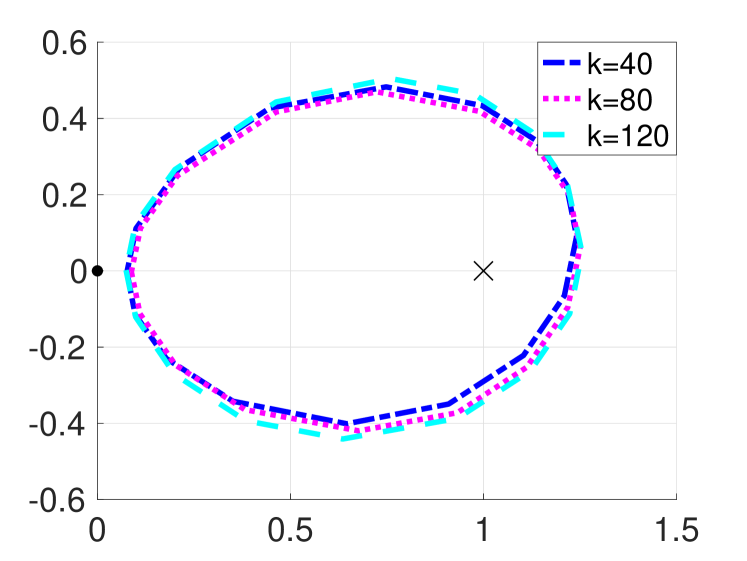
(a) SORAS, $\varepsilon=k^{1.5}$

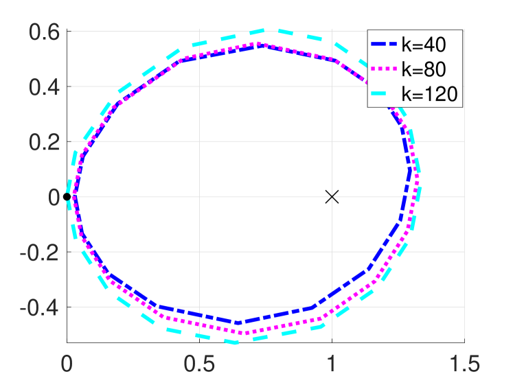
(b) SORAS, $\varepsilon=k^{1.4}$

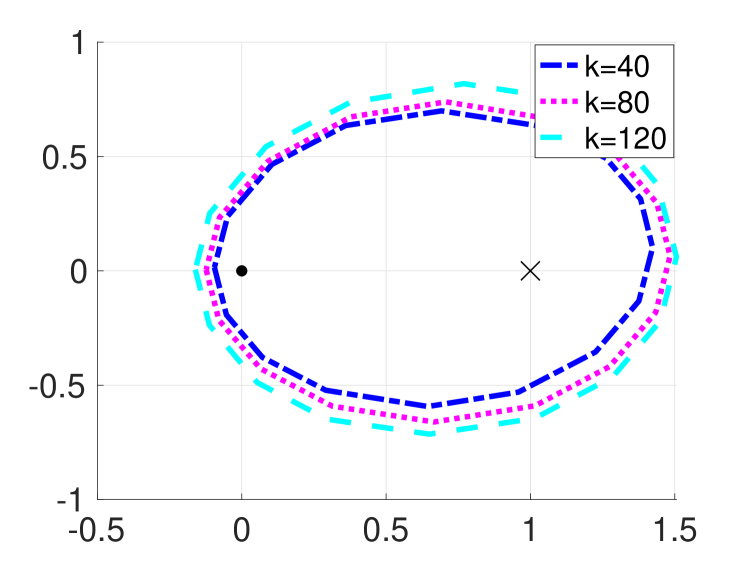
(c) SORAS, $\varepsilon=k$

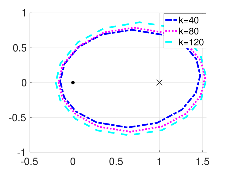
(d) SORAS, $\varepsilon=0$

Figure 1: Experiment 6.4: field of values for various $\varepsilon$ (SORAS). The origin is denoted with a bold dot and the point $1$ with an $\times$.

Experiment 6.4 (Plots of the field of values).

Linear system setting:

$$A=I,\ n=1,\text{ and }p=3$$

Preconditioner setting:

$$\text{Partition strategy 2 with }H=k^{-0.4},\delta=\frac{H}{4}$$

Corollary 5.8 used the Elman estimate to prove $k$-independent bounds on the number of GMRES iterations. This estimate requires an upper bound on the norm of the preconditioned system and a positive lower bound on the distance of its field of values from the origin and gave us a rigorous result about the $k$-independence of GMRES iterations for absorptive problems. In this experiment we illustrate two things: (i) that our estimates for the field of values are sharp in terms of their dependence on absorption, and (ii) that (given an upper bound on the norm of the preconditioned operator) the positive separation of the field of values from the origin is sufficient but appears far from necessary for good convergence of GMRES. Point (ii) is reinforced again by later experiments.

Throughout we have used the algorithm of Cowen and Harel [15] to plot the boundary of the field of values (in the inner product of $\langle\cdot,\cdot\rangle_{{\mathsf{D}}_{k}}$) for any given matrix. Recall that the field of values is a convex subset of $\mathbb{C}$. In all plots of the field of values, the origin in $\mathbb{C}$ is denoted with a bold dot, while the point at $1$ is denoted with a cross.

Figure 1 shows the boundaries of the field of values for the SORAS preconditioner in Experiment 6.4 with different choices of $\varepsilon$. Here $\delta=H/4\sim k^{-0.4}$. In Figure 1(a) $k/(|\varepsilon|\delta)=k^{-0.1}\rightarrow 0$ as $k\rightarrow\infty$ and the field of values is well away from the origin, thus confirming our estimate from Corollary 5.7. Figure 1(b) shows the case $k/(|\varepsilon|\delta)=\mathcal{O}(1)$; here the requirement (5.12) of Corollary 5.7 just fails, and we see in Figure 1(b) that the boundary of the field of values moves towards the origin as $k$ increases. For the cases shown in Figures 1(c)-1(d), $k/(|\varepsilon|\delta)$ blows up as $k$ increases and here we see that the field of values contains the origin. This experiment verifies the sharpness of the field of values estimates in §5 in terms of their dependence on $\varepsilon$. However the numerical results in Table 8 show that the preconditioners work well even in some cases where the corresponding field of values of the preconditioned problem contains the origin. For the field of values given in Figure 1(d), the preconditioner arguably still works well with increasing $k$ (6th column of Table 8). Indeed we expect that Columns 3-6 of Table 8 all correspond to fields of values that contain the origin. Thus GMRES continues to work well even in some cases where our sufficient conditions for $k$-independent iterations are violated.

We further emphasise this point by plotting in Figure 2 the field of values of the ORAS preconditioned matrices for $\varepsilon=k^{1.5}$ and $\varepsilon=0$. GMRES iteration numbers for these are given (in brackets) in Columns 2 and 6 of Table 8. In Column 2 we see convincingly $k$-independent convergence of GMRES and in Column 6 we see very good convergence; however the field of values contains the origin in all cases.

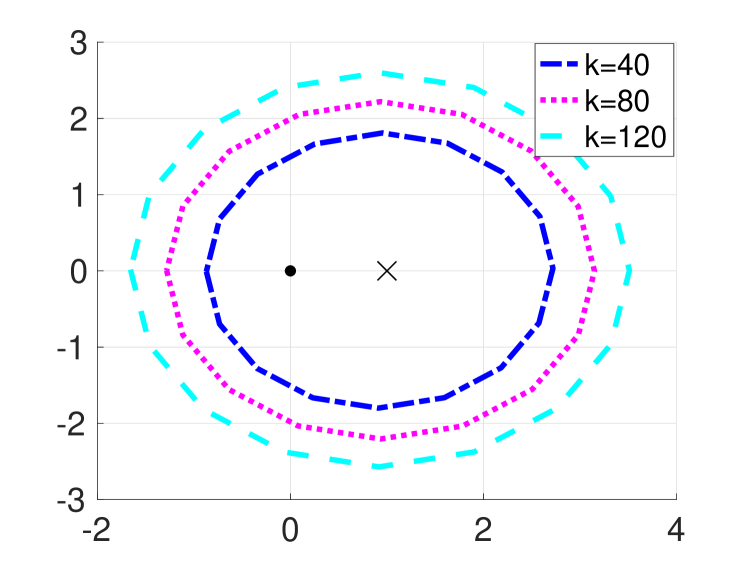
(a) ORAS, $\varepsilon=k^{1.5}$

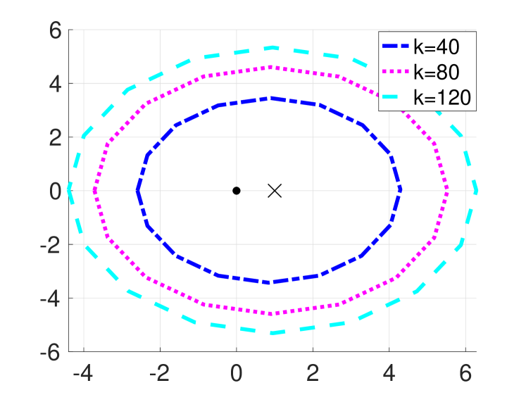
(b) ORAS, $\varepsilon=0$

Figure 2: Experiment 6.4: field of values for various $\varepsilon$ (ORAS). The origin is denoted with a bold dot and the point $1$ with an $\times$.

Experiment 6.5 (Effect of the heterogeneity of the media.).

Linear system setting:

$$\text{variable }A,\,\,n,\text{ and }p=3$$

Preconditioner setting:

$$\text{Partition strategy 2 with }H=k^{-0.4},\delta=\frac{H}{4}$$

In the domain $\Omega=(0,1)^{2}$ we introduce a penetrable obstacle that is either a disk of radius $1/4$ or a square of side length $1/2$, centred at $(1/2,1/2)$. In this experiment the penetrable obstacle corresponds to either $A$ or $n$ being variable. Although our theory allows $A$ to be a matrix, in these experiments it is scalar. Exterior to the penetrable obstacle the coefficients are $A=1$ and $n=1$. The profiles studied are shown in Figure 3. In these, grey denotes a coefficient value equal to $1$, while blue denotes a value $<1$ and red denotes a value $>1$ (with actual values to be given below). In addition:

1. Figures 3(a) and 3(d): coefficient linearly decreases from the center to the boundary of the obstacle;

2. Figures 3(b) and 3(e): coefficient linearly increases from the center to the boundary of the obstacle;

3. Figures 3(c) and 3(f): coefficient oscillates with the maximum and minimum values inside obstacle.

For the oscillating profiles in Figures 3(c) and 3(f), there are 7 layers of uniform thickness as we proceed outward from the center to the boundary of the obstacle with the maximum attained in the red layer and the minimum in the blue layer. Thus by stating the maximum and minimum values of the coefficient, all profiles are uniquely defined.

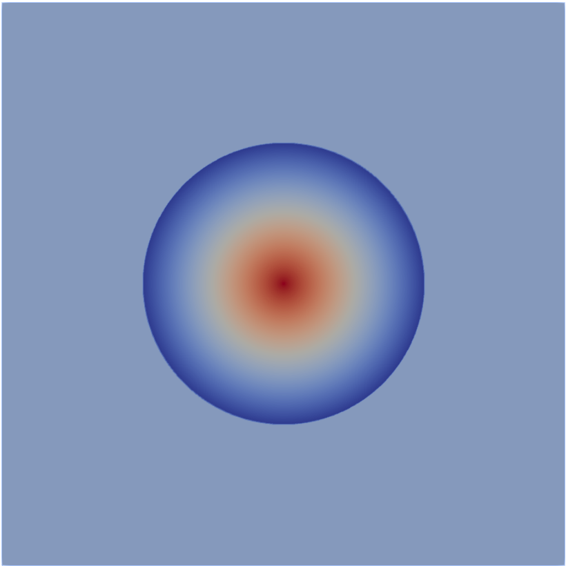
(a) maxima at center

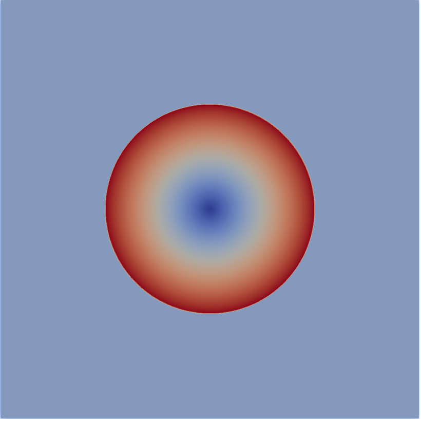
(b) minima at center

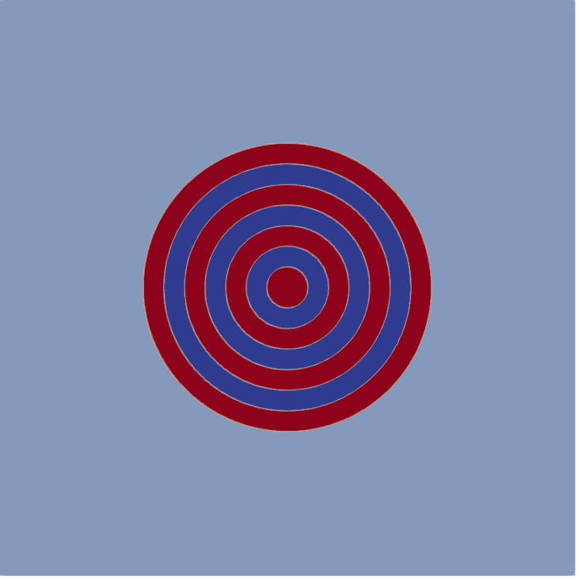
(c) oscillates

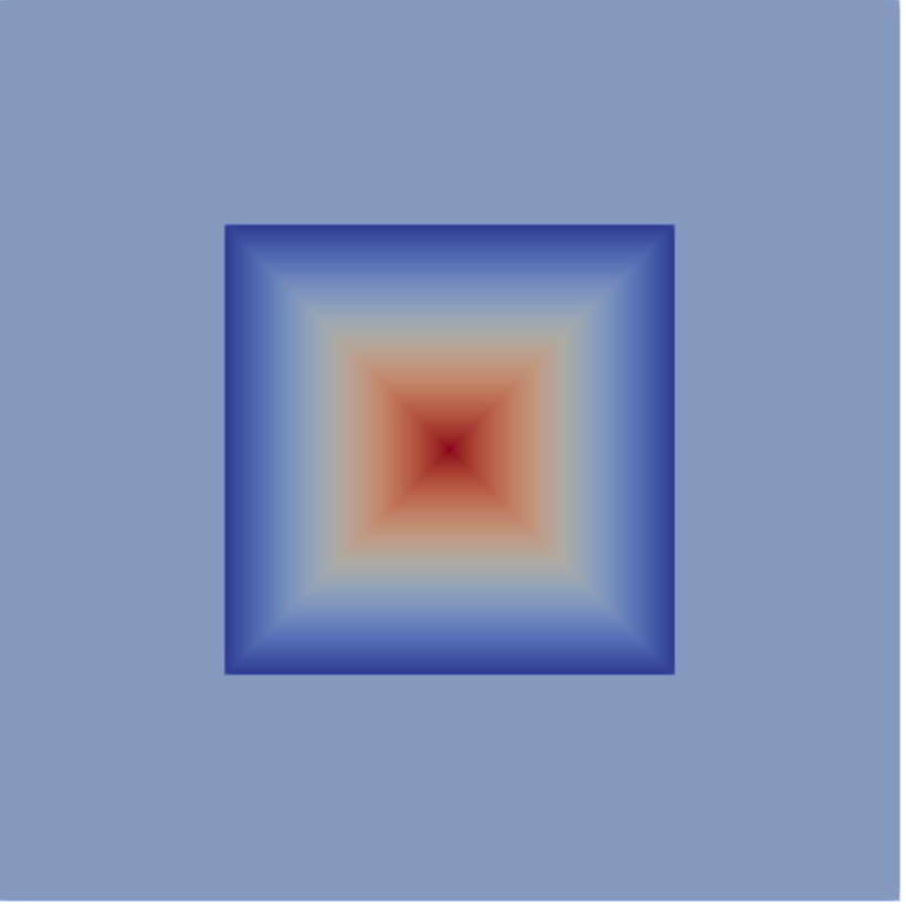
(d) maxima at center

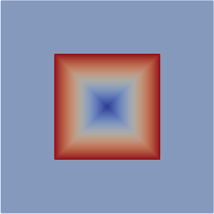
(e) minima at center

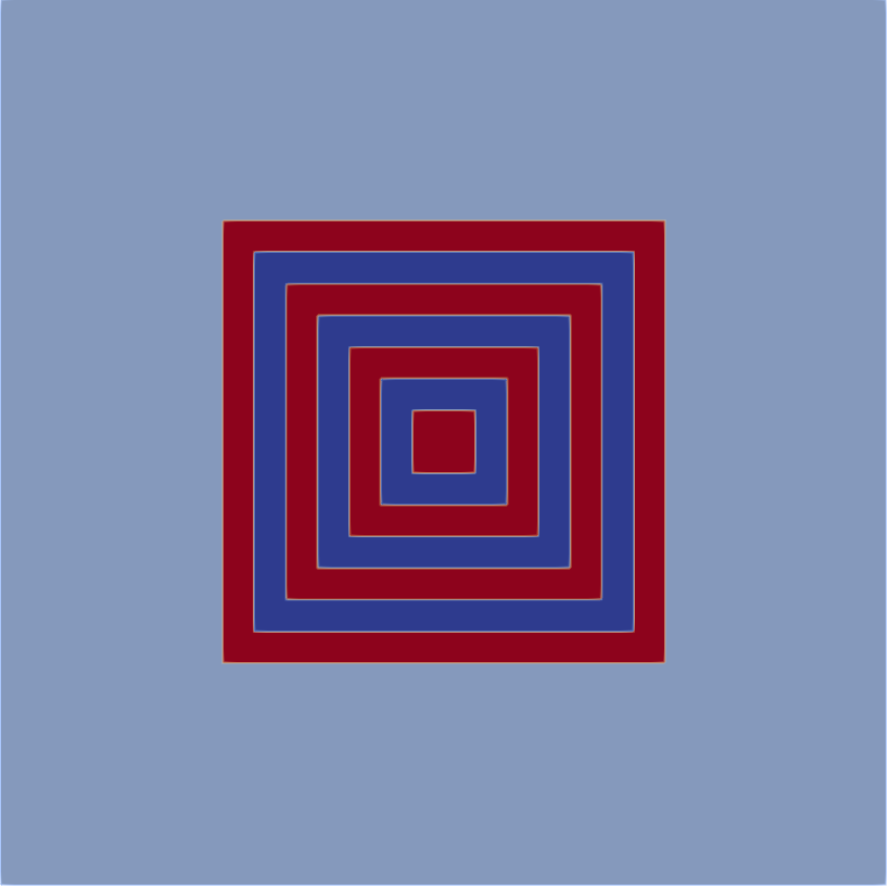
(f) oscillates

Figure 3: Different profiles for variable coefficients

Remark (Are the coefficients $A$ and $n$ arising from the profiles in Figure 3 trapping or nontrapping?).

We now describe to what extent it is known whether $A$ and $n$ arising from the profiles in Figure 3 are trapping or nontrapping. We highlight, however, (recalling the discussion and references in Remark 1.1) that even if $A$ or $n$ are trapping, we only expect to see the “bad behaviour” at certain frequencies, and indeed we do not see the extreme ill-conditioning associated with trapping for any of the frequencies used in the examples below. The summary is that

• Profile (c) is provably trapping for both $A$ and $n$.

• Profile (b) is provably trapping for $n$, and Profile (a) is provably trapping for $A$.

• We expect Profile (a) to be trapping for $n$ and Profile (b) to be trapping for $A$ (but neither is rigorously proved).

• We expect Profiles (d), (e), and (f) to be nontrapping for $n$ and $A$.

For understanding these points, recall that red indicates a coefficient value $>1$, blue indicates a coefficient value $<1$, and the coefficient away from the obstacle equals $1$.

Regarding (i): when the coefficients jump on a smooth convex interface, the problem is trapping if $n$ jumps down (moving outwards radially from the centre) or $A$ jumps up; see [57], [54, Section 6].

Regarding (ii): When $n$ is a radial function that jumps down (moving outwards from the centre) on a circular interface from a linear function to a constant, the problem is trapping by [55, §6.2], [1], similarly when $A$ is a radial function that jumps up.

Regarding (iii): when $n$ is a continuous radial function that decreases linearly and $n_{\max}$ is sufficiently large, then $n$ is trapping by [59], [30, Theorem 7.7]. We therefore expect the linear decrease in Profile (a) to mean that this profile is trapping for $n$. We cannot immediately conclude this from [59], [30, Theorem 7.7], since Profile (a) is discontinuous; however, because of the localisation of trapped waves we expect the subsequent nontrapping jump of $n$ not to affect the trapping caused by the linear decrease). Similarly, when $A$ is a continuous radial function that increases linearly and $A_{\max}$ is sufficiently large we expect Profile (b) to be trapping for $A$.

Regarding (iv): it is not yet rigorously known whether Profiles (d), (e), and (f) are trapping or nontrapping for $A$ or $n$. Indeed, all the examples of trapping described above rely on a trapped wave either circling an interface that is either radial, or smooth and convex [57], [55, §6.2], [1], or supported by a change in a radial coefficient [59], [30, Theorem 7.7]. Certainly for Profile (f) we expect $A$ and $n$ to be nontrapping, since any wave moving parallel to one of the sides of the square interfaces loses energy when it hits the next side perpendicularly; thus long-lived waves moving parallel to square interfaces cannot exist.

In Tables 9 and 10 we give the performance of GMRES for the six profiles above in the case $\varepsilon=k^{1.5}$. In Table 9, we fix $A=1$, $n_{\min}=0.02$ and $n_{\max}=50$, while in Table 10, we fix $n=1$, $A_{\min}=0.02$ and $A_{\max}=50$. We see that while the iteration counts are affected by variation in $A$, there seems no effect from the variation in $n$. In fact the performance in Table 9 is similar to the homogeneous case $A=n=1$ (Table 1). The worst cases in Table 10 are for oscillating $A$ (columns Fig 3(c) and Fig 3(f)), while $A$ increasing outwards is worse than $A$ decreasing outwards. Neverthess it does appear that iteration numbers in Table 10 are not increasing significantly with $k$.

This is a case where the field of values plots do give some indication of convergence rates. In Figure 4 we plot the field of values for the two cases of Tables 9 and 10 with $k=120$ ($n$ varying on the left and $A$ varying on the right). In this case $k/\varepsilon\delta\sim k^{-0.1}\rightarrow 0$, so Corollary 5.7 ensures that, for $k$ large enough (relative to $p$ and $\mathcal{C}_{\mathrm{local}}(A,n)$), the field of values does not include the origin. When $n$ is varying and not $A$, $\mathcal{C}_{\mathrm{local}}(A,n)$ just depends on $n_{\mathrm{min}}$ whereas when $A$ is varying and not $n$ it depends on both $A_{\mathrm{min}}$ and $A_{\mathrm{max}}$. However we also tested the case of $n_{\max}=10^{4}$, $n_{\min}=10^{-4}$ and $A=1$, in which case the iteration counts are similar to those in Table 9.

$k\backslash n$	Fig 3(a)	Fig 3(b)	Fig 3(c)	Fig 3(d)	Fig 3(e)	Fig 3(f)
40	13	13	13	13	13	13
80	12	12	12	12	12	12
120	12	12	12	12	12	12
160	12	12	12	12	12	12

Table 9: Experiment 6.5: SORAS, $\varepsilon=k^{1.5},A=1,n_{\min}=0.02,n_{\max}=50$

$k\backslash A$	Fig 3(a)	Fig 3(b)	Fig 3(c)	Fig 3(d)	Fig 3(e)	Fig 3(f)
40	20	27	47	20	29	41
80	17	30	51	18	27	46
120	21	30	54	21	30	50
160	17	26	38	19	28	46

Table 10: Experiment 6.5: SORAS, $\varepsilon=k^{1.5},n=1,A_{\min}=0.02,A_{\max}=50$

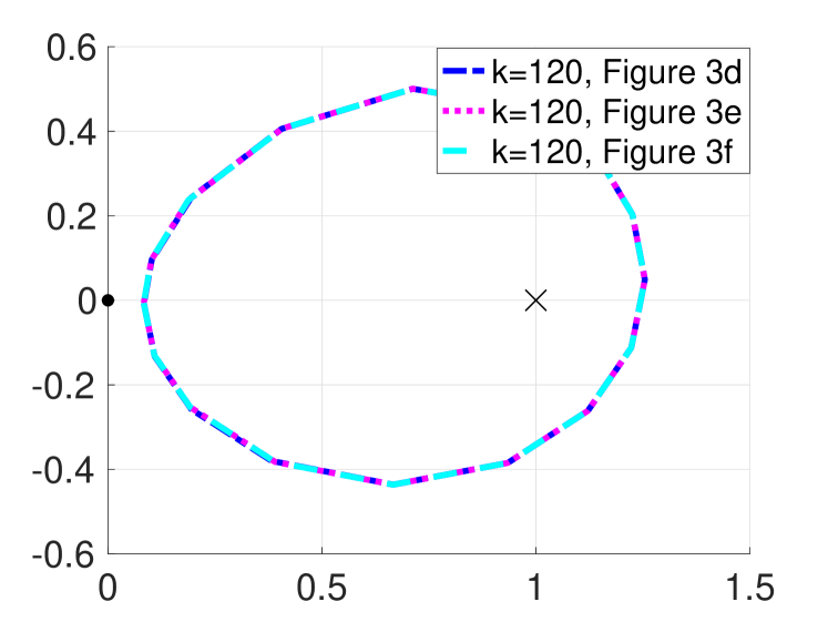
(a) $\varepsilon=k^{1.5}$, $A=1,n_{\min}=0.02,n_{\max}=50$

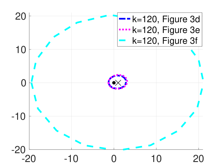
(b) $\varepsilon=k^{1.5}$, $n=1,A_{\min}=0.02,A_{\max}=50$

Figure 4: Experiment 6.5: field of values of SORAS preconditioned matrix, heterogeneous case with square obstacle, $\varepsilon=k^{1.5}$

Without absorption, the performance of GMRES becomes sensitive to variation in both $A$ and $n$. For a harder problem, in Tables 11-12, we set the quantity $\max(A_{\max},n_{\max})/(\min(A_{\min},n_{\min}))$ to $4$ and let either $A$ or $n$ vary, keeping the other fixed. The performance is worst in the cases of oscillating coefficients, while in the other cases the performance as $k$ increases is still very reasonable.

In Tables 13-14, we increase the quantity $\max(A_{\max},n_{\max})/(\min(A_{\min},n_{\min}))$ to $16$. The way the variation of $A$ affects the performance of the preconditioners does not change. But there is a big increase in GMRES iterations when the range of $n$ gets bigger. This is reflected in our estimates for the pure Helmholtz problem $\varepsilon=0$, for which the approximation of local problems (given by the estimate (4.19)) deteriorates as $n_{\max}$ increases. We also plot the field of values for the cases in Tables 13-14. The case of oscillating $A$ produces a much larger fields of values, while varying $n$ does not change the boundary of the field of values much.

$k\backslash n$	Fig 3(a)	Fig 3(b)	Fig 3(c)	Fig 3(d)	Fig 3(e)	Fig 3(f)
40	18	21	24	18	19	28
80	22	26	39	20	21	30
120	27	34	50	24	24	26
160	29	37	64	25	25	38

Table 11: Experiment 6.5: SORAS $\varepsilon=0,A=1,n_{\min}=0.5,n_{\max}=2.0$

$k\backslash A$	Fig 3(a)	Fig 3(b)	Fig 3(c)	Fig 3(d)	Fig 3(e)	Fig 3(f)
40	18	18	20	18	18	21
80	21	18	38	18	18	28
120	31	21	35	21	20	29
160	32	22	47	23	21	33

Table 12: Experiment 6.5: SORAS, $\varepsilon=0,n=1,A_{\min}=0.5,A_{\max}=2.0$

$k\backslash n$	Fig 3(a)	Fig 3(b)	Fig 3(c)	Fig 3(d)	Fig 3(e)	Fig 3(f)
40	22	26	38	21	25	32
80	35	47	44	31	28	61
120	54	56	61	41	39	67
160	61	58	55	40	39	59

Table 13: Experiment 6.5: SORAS $\varepsilon=0,A=1,n_{\min}=0.25,n_{\max}=4.0$

$k\backslash A$	Fig 3(a)	Fig 3(b)	Fig 3(c)	Fig 3(d)	Fig 3(e)	Fig 3(f)
40	19	20	23	19	19	27
80	24	21	48	19	21	40
120	29	26	49	25	21	56
160	28	24	57	25	20	57

Table 14: Experiment 6.5: SORAS, $\varepsilon=0,n=1,A_{\min}=0.25,A_{\max}=4.0$

To conclude, the observations in the heterogeneous case are:

• In the case of absorption, the performance is mainly affected by the variation of $A$, but only weakly affected by $n$;

• In the case without absorption, the performance is sensitive to the variation of both $A$ and $n$. Increasing the range of $n$ now seems to increase the iteration count more strongly than increasing the range of $A$.

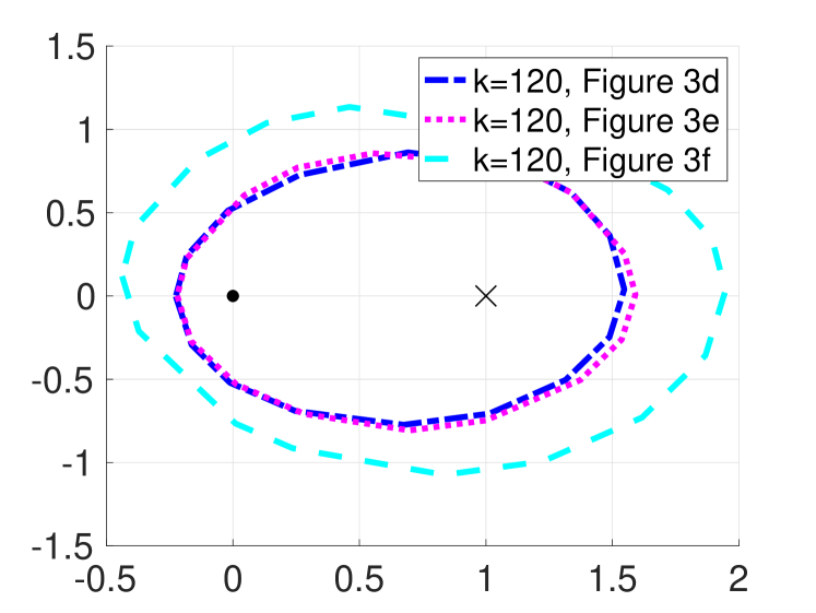
(a) $\varepsilon=0$, $A=1,n_{\min}=0.25,n_{\max}=4$

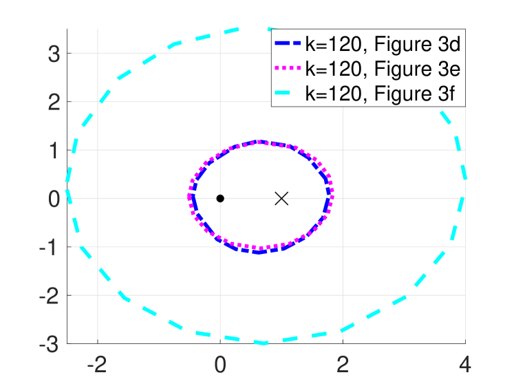
(b) $\varepsilon=0$, $n=1,A_{\min}=0.25,A_{\max}=4$

Figure 5: Experiment 6.5: SORAS, field of values in the heterogeneous case with square obstacle, $\varepsilon=0$

Experiment 6.6 (Effect of local variation of the heterogeneity.).

Linear system setting:

$$\text{variable }A,n,\text{ and }p=3$$

Preconditioner setting:

$$\text{Partition strategy 2 with }H=\frac{1}{8},\delta=\frac{H}{4}$$

In Experiment 6.5, the number of the subdomains is $4\times 4$, $5\times 5$, $6\times 6$ and $7\times 7$ for the cases $k=40,80,120$ and $160$, respectively. Thus there always exist subdomains where both global maximum and minimum coefficient values are attained for any of the profiles in Figure 3. Here we use smaller subdomain sizes (in fact $8\times 8$) in order to illustrate the local heterogeneity dependence identified in the theory (Corollary 5.7). In the case of the linear variation profiles Figures 3(a), 3(b), 3(d), 3(e), both the maximum and minimum values of the varying coefficients cannot be attained in a single subdomain. For the oscillating profiles 3(c), 3(f), however, there always exist some subdomains capturing both extreme values. Therefore Profiles 3(c), 3(f) have worse estimates for the local contrast $\mathcal{C}_{\mathrm{local}}(A,n)$ than the others and hence yield worse estimates for the field of values. In Tables 15-16 we present the results for these profiles with $\varepsilon=0$; we see that Profiles 3(c), 3(f) have noticeably worse iteration counts than the others.

$k\backslash A$	Fig 3(a)	Fig 3(b)	Fig 3(c)	Fig 3(d)	Fig 3(e)	Fig 3(f)
40	40 (28)	41 (30)	52 (33)	42 (28)	40 (30)	64 (43)
80	46 (38)	39 (29)	103 (88)	38 (27)	36 (28)	66 (59)
120	42 (37)	32 (27)	59 (61)	31 (25)	26 (23)	68 (73)
160	35 (34)	31 (25)	73 (96)	27 (23)	24 (27)	85 (103)

Table 15: Fixed subdomains, $\varepsilon=0,n=1,A_{\min}=0.25,A_{\max}=4.0$

$k\backslash n$	Fig 3(a)	Fig 3(b)	Fig 3(c)	Fig 3(d)	Fig 3(e)	Fig 3(f)
40	48 (32)	63 (54)	73 (72)	49 (38)	57 (43)	75 (56)
80	58 (51)	75 (70)	79 (84)	52 (44)	50 (40)	103 (102)
120	73 (66)	74 (90)	90 (132)	52 (44)	45 (39)	102 (124)
160	75 (82)	69 (87)	100 (124)	48 (44)	41 (36)	59 (73)

Table 16: Fixed subdomains, $\varepsilon=0,A=1,n_{\min}=0.25,n_{\max}=4.0$

Acknowledgement:  We thank Victorita Dolean (University of Strathclyde and Université Côte d’Azur) for useful mathematical discussions and also advice on FreeFEM++. We gratefully acknowledge support from the UK Engineering and Physical Sciences Research Council Grants EP/R005591/1 (EAS) and EP/S003975/1 (SG, IGG, and EAS). This research made use of the Balena High Performance Computing (HPC) Service at the University of Bath. We thank the anonymous referees for making several penetrating remarks which have improved the manuscript.

References

- [1] S. Balac, M. Dauge, and Z. Moitier. Asymptotic expansions of whispering gallery modes in optical micro-cavities. preprint, 2019.
- [2] J. M. Ball, Y. Capdeboscq, and B. Tsering-Xiao. On uniqueness for time harmonic anisotropic Maxwell’s equations with piecewise regular coefficients. Mathematical Models and Methods in Applied Sciences, 22(11):1250036, 2012.
- [3] C. Bardos, G. Lebeau, and J. Rauch. Sharp sufficient conditions for the observation, control, and stabilization of waves from the boundary. SIAM J. Control Optim., 30:1024–1065, 1992.
- [4] H. Barucq, T. Chaumont-Frelet, and C. Gout. Stability analysis of heterogeneous Helmholtz problems and finite element solution based on propagation media approximation. Math. Comp., 86(307):2129–2157, 2017.
- [5] D. Baskin, E. A. Spence, and J. Wunsch. Sharp high-frequency estimates for the Helmholtz equation and applications to boundary integral equations. SIAM Journal on Mathematical Analysis, 48(1):229–267, 2016.
- [6] B. Beckermann, S. A. Goreinov, and E. E. Tyrtyshnikov. Some remarks on the Elman estimate for GMRES. SIAM journal on Matrix Analysis and Applications, 27(3):772–778, 2006.
- [7] T. Betcke, S. N. Chandler-Wilde, I. G. Graham, S. Langdon, and M. Lindner. Condition number estimates for combined potential boundary integral operators in acoustics and their boundary element discretisation. Numerical Methods for Partial Differential Equations, 27(1):31–69, 2011.
- [8] M. Bonazzoli, X. Claeys, F. Nataf, and P.-H. Tournier. Analysis of the SORAS domain decomposition preconditioner for non-self-adjoint or indefinite problems. arXiv preprint 2003.09251, 2020.
- [9] M. Bonazzoli, V. Dolean, I. G. Graham, E. A. Spence, and P.-H. Tournier. Two-level preconditioners for the Helmholtz equation. Domain Decomposition Methods in Science and Engineering XXIV, 2018.
- [10] M. Bonazzoli, V. Dolean, I. G. Graham, E. A. Spence, and P.-H. Tournier. Domain decomposition preconditioning for the high-frequency time-harmonic Maxwell equations with absorption. Math. Comp., 88:2559–2604, 2019.
- [11] S. C. Brenner and L. R. Scott. The Mathematical Theory of Finite Element Methods, volume 15 of Texts in Applied Mathathematics. Springer Science+Business Media, New York, 3rd edition, 2008.
- [12] T. Chaumont-Frelet. On high order methods for the heterogeneous Helmholtz equation. Computers & Mathematics with Applications, 72(9):2203–2225, 2016.
- [13] T. Chaumont-Frelet and S. Nicaise. Wavenumber explicit convergence analysis for finite element discretizations of general wave propagation problem. IMA J. Num. Anal., https://doi.org/10.1093/imanum/drz020, 2019.
- [14] Z. Chen and X. Xiang. A source transfer domain decomposition method for Helmholtz equations in unbounded domain. SIAM J. Num. Anal., 51(4):2331–2356, 2013.
- [15] C. C. Cowen and E. Harel. An effective algorithm for computing the numerical range, 1995. Unpublished manuscript.
- [16] V. Dolean, P. Jolivet, and F. Nataf. An introduction to domain decomposition methods: algorithms, theory, and parallel implementation. SIAM, 2015.
- [17] Y. Du and H. Wu. Preasymptotic error analysis of higher order FEM and CIP-FEM for Helmholtz equation with high wavenumber. SIAM J. Numer. Anal., 53:782–804, 2015.
- [18] J. J. Duistermaat and L. Hörmander. Fourier integral operators. II. Acta mathematica, 128(1):183–269, 1972.
- [19] S. C. Eisenstat, H. C. Elman, and M. H. Schultz. Variational iterative methods for nonsymmetric systems of linear equations. SIAM J. Numer. Anal., pages 345–357, 1983.
- [20] H. C. Elman. Iterative Methods for Sparse Nonsymmetric Systems of Linear Equations. PhD thesis, Yale University, 1982.
- [21] B. Engquist and L. Ying. Sweeping preconditioner for the Helmholtz equation: hierarchical matrix representation. Comm. Pure Appl. Math., 64:697–735, 2011.
- [22] B. Engquist and L. Ying. Sweeping preconditioner for the Helmholtz equation: moving perfectly matched layers. Multiscale. Model. Simul., 9:686–710, 2011.
- [23] Y. A. Erlangga, C. W. Oosterlee, and C. Vuik. A novel multigrid based precconditioner for heterogeneous Helmholtz problems. SIAM J. Sci. Comp., 27:1471–1492, 2006.
- [24] Y. A. Erlangga, L. G. Ramos, and R. Nabben. The multilevel Krylov-multigrid method for the Helmholtz equation preconditioned by the shifted Laplacian. In Modern Solvers for Helmholtz Problems, pages 113–139. Springer, 2017.
- [25] Y. A. Erlangga, C. Vuik, and C. W. Oosterlee. On a class of preconditioners for solving the Helmholtz equation. Appl. Numer. Math., 50(3):409–425, 2004.
- [26] J. Galkowski, E. A. Spence, and J. Wunsch. Optimal constants in nontrapping resolvent estimates. Pure and Applied Analysis, 2(1):157–202, 2020.
- [27] M. J. Gander, I. G. Graham, and E. A. Spence. Applying GMRES to the Helmholtz equation with shifted Laplacian preconditioning: What is the largest shift for which wavenumber-independent convergence is guaranteed? Numer. Math., 131(3):567–614, 2015.
- [28] M.J. Gander and H. Zhang. A class of iterative solvers for the Helmholtz equation: factorizations, sweeping preconditioners, source transfer, single layer potentials, polarized traces, and optimized Schwarz methods. SIAM Review, 61(1):3–76, 2019.
- [29] M. Ganesh and C. Morgenstern. A coercive heterogeneous media Helmholtz model: formulation, wavenumber-explicit analysis, and preconditioned high-order FEM. Numerical Algorithms, pages 1–47, 2019.
- [30] I. G. Graham, O. R. Pembery, and E. A. Spence. The Helmholtz equation in heterogeneous media: a priori bounds, well-posedness, and resonances. Journal of Differential Equations, 266(6):2869–2923, 2019.
- [31] I. G. Graham and S. A. Sauter. Stability and finite element error analysis for the Helmholtz equation with variable coefficients. Mathematics of Computation, 89(321):105–138, 2020.
- [32] I. G. Graham, E. A. Spence, and E. Vainikko. Domain decomposition preconditioning for high-frequency Helmholtz problems with absorption. Math. Comp., 86(307):2089–2127, 2017.
- [33] I. G. Graham, E. A. Spence, and E. Vainikko. Recent results on domain decomposition preconditioning for the high-frequency Helmholtz equation using absorption. In Domenico Lahaye, Jok Tang, and Kees Vuik, editors, Modern solvers for Helmholtz problems. Birkhauser series in Geosystems Mathematics, 2017.
- [34] I. G. Graham, E. A. Spence, and J. Zou. Domain Decomposition with local impedance conditions for the Helmholtz equation. to appear in SIAM J Numer. Anal., arXiv:1806.03731, 2020.
- [35] P. Grisvard. Elliptic Problems in Nonsmooth Domains. Pitman, Boston, 1985.
- [36] S. Güttel and J. Pestana. Some observations on weighted GMRES. Numerical Algorithms, 67(4):733–752, 2014.
- [37] F. Hecht. Freefem++ manual (version 3.58-1), 2019.
- [38] U. Hetmaniuk. Stability estimates for a class of Helmholtz problems. Commun. Math. Sci, 5(3):665–678, 2007.
- [39] L. Hörmander. The analysis of linear partial differential operators III: pseudo-differential operators. Springer, 1985.
- [40] F. Ihlenburg and I. Babuska. Finite element solution of the Helmholtz equation with high wave number part II: the version of the FEM. SIAM J. Numer. Anal., 34(1):315–358, 1997.
- [41] F. Ihlenburg and I. Babuška. Dispersion analysis and error estimation of Galerkin finite element methods for the Helmholtz equation. Int. J. Numer. Meth. Eng., 38, Issue 22:3745–3774, 1995.
- [42] J-H. Kimn and M. Sarkis. Restricted overlapping balancing domain decomposition methods and restricted coarse problems for the Helmholtz problem. Comput. Method Appl. M., 196(8):1507–1514, 2007.
- [43] D. Lafontaine, E. A. Spence, and J. Wunsch. A sharp relative-error bound for the Helmholtz -fem at high frequency. arXiv preprint 1911.11093, 2019.
- [44] D. Lafontaine, E. A. Spence, and J. Wunsch. For most frequencies, strong trapping has a weak effect in frequency-domain scattering. arXiv preprint arXiv:1903.12172, 2019.
- [45] D. Lahaye, J. Tang, and K. Vuik, editors. Modern solvers for Helmholtz problems. Birkhauser series in Geosystems Mathematics, 2017.
- [46] W. C. H. McLean. Strongly elliptic systems and boundary integral equations. Cambridge University Press, 2000.
- [47] J. M. Melenk. On generalized finite element methods. PhD thesis, The University of Maryland, 1995.
- [48] J. M. Melenk and S. Sauter. Convergence analysis for finite element discretizations of the Helmholtz equation with Dirichlet-to-Neumann boundary conditions. Math. Comp, 79(272):1871–1914, 2010.
- [49] J. M. Melenk and S. Sauter. Wavenumber explicit convergence analysis for Galerkin discretizations of the Helmholtz equation. SIAM J. Numer. Anal., 49:1210–1243, 2011.
- [50] J. M. Melenk, S. A. Sauter, and C. Torres. Wave number-Explicit Analysis for Galerkin Discretizations of Lossy Helmholtz Problems. arXiv preprint arXiv:1904.00207, 2019.
- [51] R. B. Melrose and J. Sjöstrand. Singularities of boundary value problems. i. Communications on Pure and Applied Mathematics, 31(5):593–617, 1978.
- [52] R. B. Melrose and J. Sjöstrand. Singularities of boundary value problems. ii. Communications on Pure and Applied Mathematics, 35(2):129–168, 1982.
- [53] A. Moiola and E. A. Spence. Is the Helmholtz equation really sign-indefinite? SIAM Rev., 56(2):274–312, 2014.
- [54] A. Moiola and E. A. Spence. Acoustic transmission problems: wavenumber-explicit bounds and resonance-free regions. Math. Models Methods Appl. Sci., 29(2):317–354, 2019.
- [55] Z. Moitier. Étude mathématique et numérique des résonances dans une micro-cavité optique. PhD thesis, Universit’e de Rennes 1, 2019.
- [56] O. R. Pembery. The Helmholtz Equation in Heterogeneous and Random Media: Analysis and Numerics. PhD thesis, University of Bath, 2019.
- [57] G. Popov and G. Vodev. Resonances Near the Real Axis for Transparent Obstacles. Communications in Mathematical Physics, 207(2):411–438, 1999.
- [58] J. Poulson, B. Engquist, S. Li, and L. Ying. A parallel sweeping preconditioner for heterogeneous 3d Helmholtz equations. SIAM J. Sci. Comp., 35(3):C194–C212, 2013.
- [59] J. V. Ralston. Trapped Rays in Spherically Symmetric Media and Poles of the Scattering Matrix. Comm. Pure Appl. Math., 24(4):571–582, 1971.
- [60] S. Sauter and C. Torres. Stability estimate for the Helmholtz equation with rapidly jumping coefficients. Zeitschrift für angewandte Mathematik und Physik, 69(6):139, 2018.
- [61] S. A. Sauter. A refined finite element convergence theory for highly indefinite Helmholtz problems. Computing, 78(2):101–115, 2006.
- [62] S. A. Sauter and C. Schwab. Boundary Element Methods. Springer-Verlag, Berlin, 2011.
- [63] A. H. Sheikh, D. Lahaye, L. G. Ramos, R. Nabben, and C. Vuik. Accelerating the shifted Laplace preconditioner for the Helmholtz equation by multilevel deflation. J. Comp. Phys., 322:473–490, 2016.
- [64] A. St-Cyr, M. J. Gander, and S. J. Thomas. Optimized multiplicative, additive, and restricted additive Schwarz preconditioning. SIAM Journal on Scientific Computing, 29(6):2402–2425, 2007.
- [65] M. Taus, L. Zepeda-Núñez, R. J. Hewett, and L. Demanet. L-Sweeps: A scalable, parallel preconditioner for the high-frequency Helmholtz equation. arXiv preprint arXiv:1909.01467, 2019.
- [66] A. Toselli and O. Widlund. Domain Decomposition Methods: Algorithms and Theory. Springer, 2005.
- [67] P. H. Tournier, I. Aliferis, M. Bonazzoli, M. de Buhan, M. Darbas, V. Dolean, F. Hecht, P. Jolivet, I. El Kanfoud, C. Migliaccio, F. Nataf, Ch. Pichot, and S. Semenov. Microwave tomographic imaging of cerebro vascular accidents by using high-performance computing. Parallel Computing, 2019.
- [68] H. Wu. Pre-asymptotic error analysis of CIP-FEM and FEM for the Helmholtz equation with high wave number. Part I: linear version. IMA J. Numer. Anal., 34(3):1266–1288, 2014.
- [69] L. Zepeda-Núñez and L. Demanet. The method of polarized traces for the 2D Helmholtz equation. J. Comp. Phys., 308:347–388, 2016.
- [70] L. Zepeda-Núñez and L. Demanet. Nested domain decomposition with polarized traces for the 2D Helmholtz equation. SIAM J. Sci. Comp., 48:B942–B981, 2018.
- [71] L. Zhu and H. Wu. Preasymptotic error analysis of CIP-FEM and FEM for Helmholtz equation with high wave number. Part II: version. SIAM J. Numer. Anal., 51(3):1828–1852, 2013.
- [72] M. Zworski. Semiclassical analysis. American Mathematical Society Providence, RI, 2012.