Generalized positivity bounds on chiral perturbation theory

Abstract

Recently, a new set of positivity bounds with $t$ derivatives have been discovered. We explore the generic features of these generalized positivity bounds with loop amplitudes and apply these bounds to constrain the parameters in chiral perturbation theory up to the next-to-next-to-leading order. We show that the generalized positivity bounds give rise to stronger constraints on the $\bar{l}_{i}$ constants, compared to the existing axiomatic bounds. The parameter space of the $b_{i}$ constants is constrained by the generalized positivity bounds to be a convex region that is enclosed for many sections of the total space. We also show that the improved version of these positivity bounds can further enhance the constraints on the parameters. The often used Padé unitarization method however does not improve the analyticity of the amplitudes in the chiral perturbation theory at low energies.

1 Introduction

Chiral perturbation theory (ChPT) is one of the oldest and most widely studied effective field theories (EFTs) Weinberg:1966kf ; Li:1971vr ; Gasser:1983yg ; Gasser:1984gg ; Pich:1995bw ; Scherer:2002tk ; Bernard:2006gx . It is the low energy description of quantum chromodynamics (QCD), which is perturbative at high energies but strongly coupled at low energies, giving rise to the vast richness of hadron physics. The essential feature of the theory is that a chiral symmetry group, a product of two groups of the same structure, is spontaneously (and often mildly explicitly) broken down to the diagonal subgroup, which generates a nonlinear realization of the chiral symmetry. The structure of ChPT thus is largely determined by the nonlinearly realized symmetry Weinberg:1966kf ; Coleman:1969sm ; Callan:1969sn . Because of the universal structure, ChPT is also relevant for other physical scenarios as long the underlying symmetry breaking pattern is the same. Indeed, the SU(2) ChPT was also widely used as a low energy EFT for the electroweak symmetry breaking before the discovery of the light Higgs boson (see, e.g., Dobado:1990jy ; Distler:2006if ).

Although the construction of higher dimensional operators of an EFT is determined by the symmetry of the system, there are often many of them that are relevant for a given problem. Each of these operators is accompanied by a Wilson coefficient or low energy constant (LEC). The number of LECs proliferates very quickly with the dimension of the operators, so if the LECs are allowed to take any values, the parameter space of the EFT is very large. However, the LECs are not allowed to take arbitrary values if one is to assume the ultraviolet (UV) completion of the EFT satisfies axiomatic principles of quantum field theory or the scattering amplitude such as Lorentz invariance, unitarity, locality, crossing symmetry and analyticity. In particular, there are the so called positivity bounds which the LECs must satisfy Pham:1985cr ; Pennington:1994kc ; Ananthanarayan:1994hf ; Comellas:1995hq ; Dita:1998mh ; Adams:2006sv . The simplest positivity bound (see, e.g., Adams:2006sv ) states that the second $s$ derivative ($s,t,u$ being the conventional Mandelstam variables) of the pole subtracted scattering amplitude has to be positive. At low energies, the scattering amplitude can be well described by the LECs. As a result, the LECs are constrained by positivity bounds. This bound utilizes the optical theorem that is valid in the forward scattering limit, but the extension away from the forward limit is also possible Dita:1998mh ; Manohar:2008tc ; Mateu:2008gv ; Nicolis:2009qm ; Bellazzini:2016xrt . Recently, an infinite set of generalized positivity bounds have been discovered deRham:2017avq , which makes use of the simple fact that arbitrary numbers of $t$ derivatives on the imaginary part of the amplitude is positive at and away from the forward limit, though quite a few technical points need to be resolved for the generalization of these bounds for particles with spin deRham:2017zjm . We will briefly review the derivation of the generalized positivity bounds in Section 3.2 for the case of multiple scalars. Recently, there has been a renewed interest in applying positivity bounds, the forward limit bound and its generalizations, in various EFTs from particle physics and cosmology deRham:2018qqo ; deRham:2017imi ; Zhang:2018shp ; Bi:2019phv ; Remmen:2019cyz ; Bellazzini:2018paj ; Baumann:2015nta ; Bellazzini:2015cra ; Cheung:2016yqr ; Cheung:2016wjt ; Bellazzini:2017fep ; Bonifacio:2016wcb ; Hinterbichler:2017qyt ; Bonifacio:2017nnt ; Bellazzini:2017bkb ; Bonifacio:2018vzv ; Bellazzini:2019xts ; Melville:2019wyy ; deRham:2019ctd ; Alberte:2019xfh ; Alberte:2019zhd ; Ye:2019oxx ; Herrero-Valea:2019hde .

Chiral perturbation theory often serves as an exemplary EFT where features of EFTs are shown with or referred to, and as a test ground where new ideas are applied up on. In this paper, we shall apply the newly discovered generalized positivity bounds to ChPT for $\pi\pi$ scatterings. The purpose is twofold. Positivity bounds have been previously used to constrain the LECs in ChPT Pennington:1994kc ; Ananthanarayan:1994hf ; Dita:1998mh ; Distler:2006if ; Manohar:2008tc ; Mateu:2008gv (see also Refs. Sanz-Cillero:2013ipa ; Du:2016tgp for applications to ChPT with matter fields). In terms of the generalized positivity bounds of Refs. deRham:2017avq ; deRham:2017zjm , the earlier bounds are roughly the lowest order bound with only two $s$ derivatives in an infinite set of bounds with the new ingredients of arbitrary numbers of $t$ (and $s$) derivatives. Another new ingredient that one may add into the generalized bounds is the use of the improved bounds, where the low energy part of the dispersion integral is subtracted to improve the strength of the bounds. With these new ingredients, it is of interest to see how the generalized positivity bounds can improve the previous bounds on the LECs, and we will see that, indeed, the improvements are obvious, as will be shown in a number of ways. Secondly, we also use ChPT to uncover some salient properties of generalized positivity bounds for an EFT amplitude computed to higher loops. This is interesting despite previous applications of the generalized bounds in other models, as most previous applications of generalized positivity bounds are for tree level amplitudes in cosmology, where high derivative interactions can provide high momentum powers in the amplitude already at tree level. Particularly, we will explore the properties of the improved version of the generalized bounds with an explicit high-loop amplitude.

The rest of the paper is organized as follows: We start by introducing ChPT and the amplitudes for the $\pi\pi$ scattering processes in Section 2, with some long formulas of the amplitudes presented in Appendix A. In Section 3, we briefly review how to derive the generalized positivity bounds, the $Y$ bounds and the improved version. In Section 4, we first explore the structure of the infinite set of the $Y$ bounds, charting out the strengths of the different bounds and preparing for the later applications, and then use the strongest bounds to constrain the $\bar{l}_{i}$ and $b_{i}$ constants, which are the LECs in the next-to-leading order (NLO) chiral Lagrangian and combinations of the NLO and the next-to-next-to-leading (NNLO) LECs, respectively; part of the results (the 3D sections) are deferred to Appendix B. In Section 5, we discuss the structure of the improved $Y$ bounds and use them to extract the energy scale where ChPT breaks down and, more importantly, to enhance the constraints on the $\bar{l}_{i}$ and $b_{i}$ constants; we also show that the Padé unitarized amplitude has worse analytical properties than the original amplitude. We conclude in Section 6.

2 Chiral perturbation theory

Chiral perturbation theory is a low energy EFT of a field theory with (approximate) chiral symmetry group ${\rm G}_{L}\times{\rm G}_{R}$ that is spontaneously broken to the diagonal vector subgroup ${\rm G}_{V}$. The chiral symmetry is often approximate because it may be explicitly broken. For example, in QCD, it is explicitly broken by the quark mass terms (which in turn come from spontaneous breaking of other symmetries), so the degrees of the freedom associated with the breaking are pseudo-Goldstone pseudoscalars, called pions, and in this paper we only consider pion scatterings. One of the simplest chiral EFTs is where the chiral symmetry ${\rm SU}(2)_{L}\times{\rm SU}(2)_{R}$ is spontaneously broken to ${\rm SU}(2)_{V}$, which contains 3 pseudoscalars $\pi^{a}$. This model is the prototype of modern EFTs and has been extensively used to describe the low-energy dynamics of QCD involving the lightest $u$ and $d$ quarks Weinberg:1966kf ; Li:1971vr ; Gasser:1983yg ; Pich:1995bw ; Scherer:2002tk ; Bernard:2006gx . It was also used to parametrize possible symmetry breaking patterns of electroweak interactions in the limit of a heavy Higgs Appelquist:1980vg ; Longhitano:1980tm ; Longhitano:1980iz ; Herrero:1993nc ; now, with the discovery of a light Higgs, it has also been extended to include the light Higgs explicitly Buchalla:2012qq ; Buchalla:2013rka ; Alonso:2012px ; Guo:2015isa ; Buchalla:2017jlu ; Alonso:2017tdy ; Jenkins:2017dyc (for a review see Ref. Pich:2018ltt ).

The quark mass terms explicitly break the chiral symmetry, but one may add the Stückelberg or spurion fields to introduce the same symmetry breaking pattern into the effective Lagrangian, and then the chiral Lagrangian can be systematically obtained by the coset construction order by order in positive powers of the momenta and the quark masses. In the standard ChPT power counting, each insertion of the light quark mass matrix is counted as order $\mathcal{O}(p^{2})$ with $p$ the typical small momentum. For ChPT without any matter field, the leading order is $\mathcal{O}(p^{2})$. Using the sigma model parametrization, the basic building blocks for pion scatterings in the isospin symmetry limit are given by

$$U=\sqrt{1-\frac{\pi^{a}\pi^{a}}{F^{2}}}\mathbf{1}+i\frac{\pi^{a}\tau^{a}}{F}~{}~{}~{}~{}{\rm and}~{}~{}~{}~{}\chi=M^{2}\mathbf{1},$$ (1)

where $F$ and $M$, being positive constants, are the pion decay constant in the chiral limit and the leading order pion mass, respectively, ${\tau}^{a}$ is the Pauli matrix, $\mathbf{1}$ is the $2\times 2$ identity matrix and the summation for the repeated index $a$ from 1 to 3 is implied. Taking the square root of matrix $U$: $u=\sqrt{U}$, we can construct the following Hermitian matrices

$$u_{\mu}=iu^{\dagger}\partial_{\mu}Uu^{\dagger}=u_{\mu}^{\dagger},~{}~{}~{}{\rm and}~{}~{}~{}~{}\chi_{+}=u^{\dagger}\chi u^{\dagger}+u\chi^{\dagger}u=\chi_{+}^{\dagger}.$$ (2)

Then the chiral Lagrangian needed to calculate the pion scatterings up to $\mathcal{O}(p^{6})$, the next-to-next-to leading order, is Gasser:1983yg ; Bijnens:1997vq

$$\mathcal{L}_{\mathrm{ChPT}} =\mathcal{L}_{2}+\mathcal{L}_{4}+\mathcal{L}_{6}$$ (3)

$$=\frac{F^{2}}{4}\left\langle u_{\mu}u^{\mu}+\chi_{+}\right\rangle+\frac{l_{1}}{4}\left\langle u^{\mu}u_{\mu}\right\rangle^{2}+\frac{l_{2}}{4}\left\langle u_{\mu}u_{\nu}\right\rangle\left\langle u^{\mu}u^{\nu}\right\rangle+\frac{l_{3}}{16}\left\langle\chi_{+}\right\rangle^{2}+\sum_{i}c_{i}Y_{i},$$ (4)

where $\left\langle~{}\right\rangle$ denotes taking the trace of the matrix in the flavor space, $l_{i}$ and $c_{i}$ are the LECs in the $\mathcal{O}(p^{4})$ and $\mathcal{O}(p^{6})$ Lagrangians, respectively, and the $Y_{i}$ operators can be found in Table 2 of Ref. Bijnens:1999sh . The amplitude of $\pi\pi$ scatterings have been calculated up to two loops Bijnens:1995yn ; Bijnens:1997vq , which for the $\pi^{a}\pi^{b}\to\pi^{c}\pi^{d}$ scattering is given by

$$T_{ab\rightarrow cd}(s,t,u)=A(s,t,u)\delta^{ab}\delta^{cd}+A(t,s,u)\delta^{ac}\delta^{bd}+A(u,t,s)\delta^{ad}\delta^{bc},$$ (5)

with

$$A(s,t,u) =x_{2}[s-1]+x_{2}^{2}\left[b_{1}+b_{2}s+b_{3}s^{2}+b_{4}(t-u)^{2}\right]$$

$$~{}~{}~{}+x_{2}^{2}\left[F^{(1)}(s)+G^{(1)}(s,t)+G^{(1)}(s,u)\right]+x_{2}^{3}\left[b_{5}s^{3}+b_{6}s(t-u)^{2}\right]$$

$$~{}~{}~{}+x_{2}^{3}\left[F^{(2)}(s)+G^{(2)}(s,t)+G^{(2)}(s,u)\right]+O\left(x_{2}^{4}\right),$$ (6)

where $x_{2}={M_{\pi}^{2}}/{F_{\pi}^{2}}$ is the power counting parameter, with $M_{\pi}$ the pion mass and $F_{\pi}$ the pion decay constant, and $s,t,u$ are the dimensionless Mandelstam variables

$$s=\frac{\left(p_{a}+p_{b}\right)^{2}}{M_{\pi}^{2}},~{}t=\frac{\left(p_{a}-p_{c}\right)^{2}}{M_{\pi}^{2}},~{}u=\frac{\left(p_{a}-p_{d}\right)^{2}}{M_{\pi}^{2}}.$$ (7)

$F^{(i)}(s)$ and $G^{(i)}(s,t)$ are loop functions defined in Appendix A, and the $b_{i}$ constants are functions of the renormalised LECs $l_{i}^{r}(\mu)$ and $r_{i}^{r}(\mu)$ in $\mathcal{L}_{4}$ and $\mathcal{L}_{6}$, respectively (see Appendix A). Using the positivity bounds, we can impose bounds on the $b_{i}$ constants. For the case of QCD, we take $M_{\pi}=139.57~{}{\rm MeV}$ and $F_{\pi}=92.28(9)$ MeV Tanabashi:2018oca . Note that in the above expressions we apparently used $F_{\pi}$ or $x_{2}$ to order the EFT expansion. However, we would like to emphasize that the real perturbative expansion parameter is actually ${M_{\pi}^{2}}/\Lambda^{2}$ with $\Lambda=4\pi F_{\pi}$ Manohar:1983md .

We will consider a generic elastic scattering process $\left|\pi^{\alpha}\right\rangle+\left|\pi^{\beta}\right\rangle\rightarrow\left|\pi^{\alpha}\right\rangle+\left|\pi^{\beta}\right\rangle$ with $\left|\pi^{\alpha}\right\rangle$ and $\left|\pi^{\beta}\right\rangle$ states being superpositions of the isospin states

$$\left|\pi^{\alpha}\right\rangle =\alpha_{a}\left|\pi^{a}\right\rangle=\alpha_{1}\left|\pi^{1}\right\rangle+\alpha_{2}\left|\pi^{2}\right\rangle+\alpha_{3}\left|\pi^{3}\right\rangle,$$ (8)

$$\left|\pi^{\beta}\right\rangle =\beta_{a}\left|\pi^{a}\right\rangle=\beta_{1}\left|\pi^{1}\right\rangle+\beta_{2}\left|\pi^{2}\right\rangle+\beta_{3}\left|\pi^{3}\right\rangle,$$ (9)

where $\alpha_{a}$ and $\beta_{a}$ are arbitrary complex constants satisfying the normalized conditions: $|\alpha_{a}|^{2}=1$ and $|\beta_{a}|^{2}=1$. In this case, the scattering amplitude is given by

$$T_{\alpha\beta\rightarrow\alpha\beta}(s,t,u)=\eta_{1}A(s,t,u)+A(t,s,u)+\eta_{2}A(u,t,s),$$ (10)

with $\eta_{1}=|\alpha_{a}\beta_{a}|^{2}$ and $\eta_{2}=|\alpha_{a}\beta_{a}^{*}|^{2}$. By the Cauchy–Schwarz inequality, we have

$$0\leq{\eta}_{1}\leq 1~{}~{}{\rm and}~{}~{}0\leq\eta_{2}\leq 1.$$ (11)

As we shall see below, positivity bounds can be derived for a general elastic scattering $\left|\pi^{\alpha}\right\rangle+\left|\pi^{\beta}\right\rangle\rightarrow\left|\pi^{\alpha}\right\rangle+\left|\pi^{\beta}\right\rangle$ with general $\eta_{1}$ and $\eta_{2}$.

3 Generalized positivity bounds

The properties of the UV theory of an EFT such as unitarity, locality, analyticity and crossing symmetry can be used to derive some conditions that constrain the LECs of the EFT. A forward limit positivity bound was derived in Ref. Adams:2006sv , and this has been generalized away from the forward limit in ChPT Manohar:2008tc . In this section, we will briefly summarize the generalized positivity bounds proposed in Refs. deRham:2017avq ; deRham:2017zjm , which includes the one in Ref. Manohar:2008tc as a special case.

3.1 The $Y$ bounds

We shall use the shorthand notation $T(s,t)=T_{\alpha\beta\rightarrow\alpha\beta}(s,t,u)={\alpha}_{a}{\beta}_{b}{\alpha}_{c}^{*}{\beta}_{d}^{*}T_{ab\rightarrow cd}(s,t,u)$. By Cauchy’s integral theorem, crossing symmetry and the Froissart-Martin bound Froissart:1961ux ; Martin:1962rt ; Jin:1964zza

$$\lim_{s\rightarrow\infty}|T(s,t)|<Cs^{1+\varepsilon(t)},~{}\varepsilon(t)<1,~{}0\leq t<4,~{}C={\rm\;const},$$ (12)

we can derive a fixed-$t$ dispersion relation for the amplitude $T(s,t)$

$$B(s,t) \equiv T(s,t)-\frac{\lambda}{1-s}-\frac{\lambda}{1-t}-\frac{\lambda}{1-u}$$ (13)

$$=a(t)+\int_{4}^{\infty}\frac{\mathrm{d}\mu}{\pi\left(\mu-\mu_{p}\right)^{2}}\left[\frac{\left(s-\mu_{p}\right)^{2}}{\mu-s}\operatorname{Im}T(\mu,t)+\frac{\left(u-\mu_{p}\right)^{2}}{\mu-u}\operatorname{Im}\tilde{T}(\mu,t)\right],$$ (14)

where we have used the dimensionless Mandelstam variables defined in Eq. (7), ${\lambda}$ is a constant, the subtraction point is chosen to be $\mu_{p}=-t/2$, and the $s\leftrightarrow u$ crossed amplitude is $\tilde{T}(s,t)={\alpha}_{a}{\beta}^{*}_{b}{\alpha}_{c}^{*}{\beta}_{d}T_{ab\rightarrow cd}(s,t,u)$. Expanding the amplitude in terms of partial waves,

$$T(s,t)=16\pi\sqrt{\frac{s}{s-4}}\sum_{\ell=0}^{\infty}(2\ell+1)P_{\ell}\left(1+\frac{2t}{s-4}\right)t_{\ell}(s),$$ (15)

the partial wave unitarity requires $\left|t_{\ell}(s)\right|^{2}\leq\operatorname{Im}t_{\ell}(s)$ for $s\geq 4$. Utilizing the positivity properties of the Legendre polynomials $\mathrm{d}^{n}P_{\ell}(x=1)/\mathrm{d}x^{n}\geq 0$ for $n\geq 0$ and Martin’s extension of analyticity Martin:1965jj we can obtain deRham:2017avq

$$\frac{\mathrm{d}^{n}}{\mathrm{d}t^{n}}\operatorname{Im}T(s,t)>0,\quad s>4,\quad 0\leq t<4,\quad n\geq 0.$$ (16)

(See Appendix B of Ref. deRham:2017imi for the reason why this is a strict positivity (rather than semi-positivity) condition for a nontrivial scattering.) Since the $t$ variable is proportional to the cosine of the scattering angle, the inequality (16) essentially gives rise to constraints for all of the partial waves. The same relation holds for the $s\leftrightarrow u$ crossed amplitude $\tilde{T}(s,t)$. It is also convenient to use $v=s+t/2-2$ instead of $s$, for which we have $v=0$ when $s=u$. Thanks to the two ingredients (14) and (16), we see that if an even number of $v$ derivatives act on ${B}(s,t)$, we get a quantity that is positive definite. That is, if we define

$$B^{(2N,M)}(t)=\left.\frac{1}{M!}\partial_{v}^{2N}\partial_{t}^{M}{B}(s,t)\right|_{v=0},$$ (17)

we have $B^{(2N,0)}(t)>0$ for $N\geq 1$. $N$ needs to be greater than 0 because we need to eliminate the unknown subtraction function $a(t)$. Actually, when $M=0$, these inequalities also hold away from $v=0$, as explained in Ref. Manohar:2008tc . The same, however, is not true for the $t$ derivatives because the sign of $B^{(2N,M)}(t)$ alternates for different $M$, due to the $u$ channel part of the integrand of Eq. (14). This can be overcome if we linearly combine different $B^{(2N,M)}(t)$ and use the “relaxing” inequality of a positive integration $\int_{4}^{\infty}\mathrm{d}\mu\,(...)/({\mu}+{t}/2-2)<\int_{4}^{\infty}\mathrm{d}\mu\,(...)/\mathcal{M}^{2}$, where $(...)$ denotes a positive quantity and $\mathcal{M}^{2}=2+\frac{t}{2}$ is the minimum of $({\mu}+{t}/2-2)$. With some algebra, we can get deRham:2017avq ; deRham:2017zjm

$$Y^{(2N,M)}(t)=\sum_{r=0}^{M/2}c_{r}B^{(2(N+r),M-2r)}+\frac{1}{\mathcal{M}^{2}}\sum_{\text{even }k=0}^{(M-1)/2}(2(N+k)+1)\beta_{k}Y^{(2(N+k),M-2k-1)}>0,$$ (18)

where $N\geq 1$, $M\geq 0$, $0\leq t<4$, $Y^{(2N,0)}(t)=B^{(2N,0)}(t)$ and $c_{k}$ and $\beta_{k}$ are given by

$$c_{k}=-\sum_{r=0}^{k-1}\frac{2^{2(r-k)}c_{r}}{(2(k-r))!},\quad c_{0}=1\quad\text{ and }\quad\beta_{k}=(-1)^{k}\sum_{r=0}^{k}\frac{2^{2(r-k)-1}}{(2(k-r)+1)!}c_{r}.$$ (19)

An intriguing fact is that $c_{k}$ and $\beta_{k}$ are simply the Taylor expansion coefficients of the ${\rm sech}(x/2)$ and $\tan(x/2)$ functions, respectively deRham:2017imi . The full amplitude satisfying analyticity, unitarity and crossing symmetry is used to derive the positivity bounds derived above. However, at low energies, a decent EFT amplitude must approximate the full amplitude perturbatively to a desired accuracy by power counting, so the positivity bounds can be obtained with the EFT amplitude within that accuracy, and the bounds then translate into inequalities on the LECs.

3.2 The improved $Y$ bounds

The dispersion relation (14) integrates the imaginary part of the amplitude from $4$ to $\infty$. However, within the EFT, we can actually compute ${\rm Im}A(s,t)$ at low energies below the cutoff, so we can subtract out the low energy part of the integral to get deRham:2017imi ; Bellazzini:2016xrt ; Bellazzini:2017fep ; deRham:2017xox

$$B_{\epsilon\Lambda}(t)=B(t)-\int_{4}^{(\epsilon\Lambda)^{2}}\frac{\mathrm{d}\mu}{\pi\left(\mu-\mu_{p}\right)^{2}}\left[\frac{\left(s-\mu_{p}\right)^{2}}{\mu-s}\operatorname{Im}T(\mu,t)+\frac{\left(u-\mu_{p}\right)^{2}}{\mu-u}\operatorname{Im}\tilde{T}(\mu,t)\right],$$ (20)

where we choose $\epsilon\ll 1/M_{\pi}$ ($\epsilon\Lambda$ being dimensionless) to stay well below the cutoff. By doing so, we have assumed that the imaginary part of the amplitude can be determined with a desired accuracy below $\epsilon\Lambda$ within a given order of EFT – note that unitarity is only perturbatively satisfied in an EFT constructed from a derivative expansion. Since the integrand is positive, we can use $B_{\epsilon\Lambda}^{(2N,M)}(t)$ and go through the same steps and get

$$Y_{\epsilon\Lambda}^{(2N,M)}(t)>0.$$ (21)

where now $\mathcal{M}^{2}=\epsilon^{2}\Lambda^{2}+t/2-2$. This is an improvement compared to the $Y$ bounds in the previous subsection, because essentially the improved bounds state that $Y^{(2N,M)}$ is actually greater than a positive number, as opposed to 0 as in the original $Y$ bounds. In addition, it raises the scale of $\mathcal{M}^{2}$ from $\mathcal{O}(1)$ to $\epsilon^{2}\Lambda^{2}\gg 1$, which in turn leads to enhancement of the higher order $Y$ bounds.

4 $Y$ bounds on ChPT

As discussed in Section 3, the generalized positivity bounds are a large set of new constraints with different choices of $\{\eta_{1},\eta_{2},t,N,M\}$. Up to two loops, the LECs in ChPT are bundled in the $b_{i}$ constants and the amplitude is linear in $b_{i}$, so for a given set of $\{\eta_{1},\eta_{2},t,N,M\}$ the positivity bound is a linear inhomogeneous inequality for $b_{i}$. To get the best bounds on the LECs in ChPT, we should survey all the different choices and solve a large, principally infinite, set of inequalities, and, as we will explain later, the final bounded region has to be convex. Before doing that, we shall first explore how the positivity bounds look like for different choices of the parameters mentioned above, so as to set up a guide to proceed more effectively. Note that, for ChPT up to $\mathcal{O}(p^{6})$, despite that the analytic polynomial terms, which contain the $b_{i}$ LECs, are at most to the third power of the Mandelstam variables, the amplitude nevertheless contains complicated logarithmic functions (see Appendix A) which give rise to the $Y$ bounds with large $N,M$.

However, numerically evaluating the higher order bounds with those logarithmic functions is relatively slow, as imaginary numbers would appear and cancel later for the $s$ and $t$ values we are interested in. To alleviate this problem, we replace the logarithmic functions in the amplitude with the arc tangent functions using the identity ${\arctan}(z)=\frac{1}{2i}{\ln}(\frac{1+i\cdot z}{1-i\cdot z})$. Additionally, we shall Taylor expand the arc tangent functions at $t_{0}$ ($0<t_{0}<4$) to order $\mathcal{O}(\left(t-t_{0}\right)^{60})$, which further speeds up the numerical evaluations for large $N,M$.

4.1 Structure of the bounds

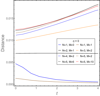
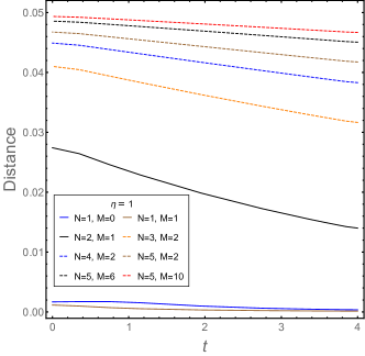
Figure 1: Distances between the bound plane and a fiducial point of $b_{i}$ of in the $(b_{1},b_{2},b_{3},b_{4},b_{5},b_{6})$ space for the cases of $\eta=0,1$. The bound plane is depicted by $Y^{(2N,M)}(t)=a_{0}+\sum_{i=1}^{6}a_{i}b_{i}=0$ for a given set of $\{\eta,t,N,M\}$. The fiducial point is taken to be the fitted values of $b_{i}$ in Eq. (33). For most bounds, the distance varies monotonically with $t$, except for $\{\eta=0,N=2,M=1\}$ and $\{\eta=1,N=1,M=0\}$, but in all of these cases the shortest distances are always at $t=0$ or $4$.

First of all, note that the $\eta_{1}$ and $\eta_{2}$ parameters appear linearly in the positivity bounds, so the strongest bounds can be obtained when $\eta_{1}$ and $\eta_{2}$ are evaluated at 0 and 1. Furthermore, in the $Y$ bounds, $\eta_{1}$ and $\eta_{2}$ always appear in the combination of

$$\eta\equiv\frac{\eta_{1}+\eta_{2}}{2}.$$ (22)

This is due to the fact that the $Y$ bounds by construction are evaluated at the $s\leftrightarrow u$ symmetric point, i.e., at $v=s+\frac{t}{2}-2=0$ (or $s=u$). To see this at a technical level, we can recast the amplitude as

$$T_{\alpha\beta\rightarrow\alpha\beta}(s,t,u)=\frac{\eta_{1}+\eta_{2}}{2}[A(s,t,u)+A(u,t,s)]+A(t,s,u)+\frac{\eta_{1}-\eta_{2}}{2}[A(s,t,u)-A(u,t,s)].$$ (23)

The $Y$ positivity bounds are just a linear combination of the $v$ and $t$ derivatives of the amplitude with $v$ evaluated at $0$. Note that the last term in the amplitude $A(s,t,u)-A(u,t,s)$ is $s\leftrightarrow u$ antisymmetric, i.e., $A(s,t,u)-A(u,t,s)$ changes its sign when $v$ goes to $-v$, so $A(s,t,u)-A(u,t,s)$ can be expanded in terms of odd powers of $v$. Thus, any even order $v$ derivatives of $A(s,t,u)-A(u,t,s)$ vanishes when evaluated at $v=0$. Since the $Y$ bounds only involve even order $v$ derivatives of the amplitude (see Eqs. (17) and (18)), this implies that $A(s,t,u)-A(u,t,s)$, thus in turn $(\eta_{1}-\eta_{2})/2$, does not contribute to the $Y$ bounds, so the $Y$ bounds only depend on $\eta$. This can also be easily checked by explicit computations. Now, since the amplitude is linear on $\eta$, we only need to consider the extremum of $\eta$, i.e., $\eta=0~{}{\rm or}~{}1$, which will give the strongest bounds for fixed $\{N,M,t\}$. That is, the strongest bounds are given by the choices of, for example, the $\pi^{1}\pi^{1}\to\pi^{1}\pi^{1}$ scattering ($\eta=1$) and the $\pi^{1}\pi^{2}\to\pi^{1}\pi^{2}$ scattering ($\eta=0$). This is probably not surprising considering the symmetry of the isospin space.

For the other continuous parameter $t$, the situation is slightly subtler. For a given set of $\{\eta,t,N,M\}$, any of the $Y$ bounds is of the form: $a_{0}+\sum_{i=1}^{6}a_{i}b_{i}>0$, which after replacing $>$ with $=$ can be viewed as a plane in the 6D space of $(b_{1},b_{2},b_{3},b_{4},b_{5},b_{6})$. Thus one may hope to devise a fiducial measure of the strength of the bound as the distance between the plane and a fiducial point. A reasonable fiducial point can be taken as the central values of the parameters determined in Ref. Colangelo:2001df using Roy’s dispersive equations with inputs from experiments (see Eq. (33)). In Figure 1, we plot how the distances of various bounds vary with $t$. We see that for the bounds with $N<6$ and $M<11$ most of the bounds monotonically increase or decrease with $t$, the only two exceptions being $\{\eta=0,N=2,M=1\}$ and $\{\eta=1,N=1,M=0\}$. Even for these two exceptional cases, the bound plane at either $t=0$ or $4$ is the nearest to the fiducial point. However, this does not mean that we can simply take $t=0$ and $t=4$ when evaluating the bounds, because the $Y$ bounds are tilted in different directions, so bounds with greater distances from the fiducial point can also contribute to the strongest bounds – the final convex region of the bounds, see Figure 2 for an example. Therefore, we shall sample the whole range of $t$ where the $Y$ bounds are valid to get the strongest bounds.

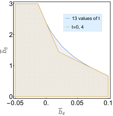
Figure 2: The positivity constraints on the parameter space of $\{b_{4},b_{6}\}$ with other $b_{i}$ set to the central values of the fit (33). The yellow region is ruled out by the $Y$ bounds with $\eta=0,t=0,4$, and is smaller than the blue region that is ruled out by the $Y$ bounds with $\eta=0$ and $13$ values of $t$.

On the other hand, for fixed $t$ and $\eta$, the lowest few $N$ and $M$ give the strongest bounds. In Figures 3 and 4, we plot the strengths of the bounds for different $\{\eta,t,N,M\}$. The color value is the rescaled value of $Y^{(2N,M)}(t)$, that is, the value of $Y^{(2N,M)}(t)/a_{0}=1+\sum_{i=1}^{6}a^{\prime}_{i}b_{i}$ with $b_{i}$ substituted by the central values of Ref. Colangelo:2001df . So in the following, we will consider bounds with $\eta=0,1,N<6,M<11$ and with different values of $t$ sampling the allowed range.

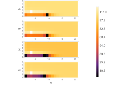
Figure 3: Rescaled values of $Y^{(2N,M)}(t)$ for $\eta=0$ and different $\{N,M\}$ at $t=4,3.5,2,0.4$ (from top to bottom). The rescaled value of $Y^{(2N,M)}(t)$ is defined as $Y^{(2N,M)}(t)/a_{0}=1+\sum_{i=1}^{6}a^{\prime}_{i}b_{i}$. The strongest bounds are given by small $N$ and $M$.

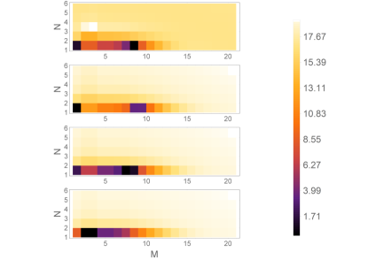
Figure 4: Similar to Figure 3 but for the case of $\eta=1$.

4.2 Bounds on $\bar{l}_{1}$ and $\bar{l}_{2}$

The scale-independent LECs $\bar{l}_{1}$ and $\bar{l}_{2}$, which are related to $l^{r}_{i}$ by

$$l_{1}^{r}=\frac{1}{96\pi^{2}}\left(\bar{l}_{1}+\ln\frac{M_{\pi}^{2}}{\mu^{2}}\right),~{}~{}~{}l_{2}^{r}=\frac{1}{48\pi^{2}}\left(\bar{l}_{2}+\ln\frac{M_{\pi}^{2}}{\mu^{2}}\right),$$ (24)

have been constrained previously using field theoretical principles Pennington:1994kc ; Ananthanarayan:1994hf ; Dita:1998mh ; Comellas:1995hq ; Manohar:2008tc . The strongest among them is given by Ref. Manohar:2008tc , which used essentially, in our notation, the $Y^{(2,0)}(t)$ positivity bound to constrain the two LECs. In this section, we will see how the bounds with $t$ or higher order $s$ derivatives can improve the constraints on $\bar{l}_{1}$ and $\bar{l}_{2}$.

To this end, we can truncate the amplitude to $\mathcal{O}(p^{4})$. That means for $b_{i}$ we only keep the leading order LECs $16\pi^{2}b_{3}=\frac{1}{3}\bar{l}_{1}+\frac{1}{6}\bar{l}_{2}-\frac{7}{12}$ and $16\pi^{2}b_{4}=\frac{1}{6}\bar{l}_{2}-\frac{5}{36}$, while $b_{1}$ and $b_{2}$ do not enter the positivity bounds. Since the leading Weinberg tree amplitude has at most linear terms in Mandelstam variables, and thus do not contribute to the positivity bounds after two $s$ derivatives, the bounds obtained are independent of the pion mass and decay constant. Thus, the bounds on $\bar{l}_{1}$ and $\bar{l}_{2}$ at one loop are universal, not just for ChPT from QCD.

Up to $\mathcal{O}(p^{4})$, the $\bar{l}_{1}$ and $\bar{l}_{2}$ coefficients only appear in the polynomial part of the amplitude, which is only up to quadratic order in Mandelstam’s variables, so one may wonder whether the higher derivative $Y$ bounds can play any role here. As we see momentarily, they do provide further constraints. This is because the higher derivative bounds are built up on the lower derivative ones which contain the $\bar{l}_{1}$ and $\bar{l}_{2}$ coefficients, as one can see from Eq. (18), and the loop logarithmic functions can contribute negatively to the positivity bounds. (By the same token, if we include the ${\cal O}(p^{6})$ contributions we will not get new constraints on $\bar{l}_{1}$ and $\bar{l}_{2}$ alone — the bounds will then contain LECs other than $\bar{l}_{1}$ and $\bar{l}_{2}$.)

Ref. Manohar:2008tc works with amplitudes for fixed total isospins. In this approach, the $s\leftrightarrow u$ crossing for a total isospin amplitude often generates terms with negative coefficients in front of the amplitudes, for which case one may not establish the positivity for the left hand cut in the fixed-$t$ dispersion relation. A linear combination of the total isospin amplitudes can overcome this problem, which allows Ref. Manohar:2008tc to apply the 2nd $s$ derivative bound for the following processes: $\pi^{0}\pi^{0}\rightarrow\pi^{0}\pi^{0}$, $\pi^{+}\pi^{0}\rightarrow\pi^{+}\pi^{0}$, $\pi^{+}\pi^{+}\rightarrow\pi^{+}\pi^{+}$. Note that the fields in the isospin basis are related to those in the Cartesian basis via $\pi^{1}=(\pi^{+}+\pi^{-})/\sqrt{2}$, $\pi^{2}=i(\pi^{+}-\pi^{-})/\sqrt{2}$ and $\pi^{3}=\pi^{0}$, while a conventional isospin basis can be chosen as $|1,+1\rangle=-\left|\pi^{+}\right\rangle$, $|1,-1\rangle=+\left|\pi^{-}\right\rangle$, $|1,0\rangle=\left|\pi^{0}\right\rangle$. The strongest bounds in that approach are given by

$$\pi^{0}\pi^{0}\rightarrow\pi^{0}\pi^{0}: ~{}~{}\bar{l}_{1}+2\bar{l}_{2}>\frac{157}{40}=3.9\pm 0.4, \text{for}~{}\eta=1,t=4,s=0,N=1,M=0,$$ (25)

$$\pi^{+}\pi^{0}\rightarrow\pi^{+}\pi^{0}: ~{}~{}\bar{l}_{2}>\frac{27}{20}=1.4\pm 0.4, \text{for}~{}\eta=0,t=4,s=0,N=1,M=0,$$ (26)

$$\pi^{+}\pi^{+}\rightarrow\pi^{+}\pi^{+}: ~{}~{}\bar{l}_{1}+3\bar{l}_{2}>5.6\pm 0.4, \text{for}~{}\eta=\frac{1}{2},t=4,s=1.114,N=1,M=0.$$ (27)

Note that the third bound above corresponds to $\eta_{1}=0$ and $\eta_{2}=1$, i.e., $\eta=1/2$ and $(\eta_{1}-\eta_{2})/2=-1/2$, so this bound is not one of the $Y$ bounds. This marks a subtle difference between the Manohar-Mateu bounds and the $s$ derivative $Y$ bounds. Previously, below Eq. (23), we have pointed out that only the parameter combination $\eta=(\eta_{1}+\eta_{2})/2$ appears in the $Y$ bounds, and since $\eta$ appears linearly in the $Y$ bounds, the strongest results can be obtained with either $\eta=0$ or $\eta=1$. This is valid because the $Y$ bounds by construction are evaluated at $v=s+\frac{t}{2}-2=0$, which is convenient for systematically obtaining all the higher order $t$ derivative bounds but does not include all possible valid values of $s$ and $t$ for the $s$ derivative bounds. Indeed, the third bound above is evaluated at $v\neq 0$ with $s=1.114$ and $t=4$, and thus not covered by the $Y$ bounds. However, as we shall see shortly, the restriction of the $Y$ bounds being evaluated at $v=0$ is well compensated by the addition of the $t$ derivative bounds, and the $Y$ bounds ultimately provide stronger bounds.

Following Manohar:2008tc , we have also added the error estimates for the bounds Eqs. (25) to (27) from the $\mathcal{O}(p^{6})$ contributions of the amplitude. There are three parts of the $\mathcal{O}(p^{6})$ contributions: tree level contribution from the $\mathcal{O}(p^{6})$ LECs, one loop contribution involving the $\mathcal{O}(p^{4})$ LECs and two loop contribution from the leading chiral Lagrangian. Here we are bounding $\bar{l}_{1}$ and $\bar{l}_{2}$, while other ${\cal O}(p^{4})$ LECs and the ${\cal O}(p^{6})$ LECs are badly known. On the other hand, the two loop contribution only depends on $M_{\pi}$ and $F_{\pi}$, which we have better control over. Assuming naturalness, one may expect that the three contributions are around the same order, so a rough estimate of the errors is to multiply the two loop contribution by a factor of 3 and take the maximum of them as a common error estimate, which is the 0.4 quoted in Eqs. (25) to (27).

In our approach, we consider a general elastic scattering $\pi^{\alpha}\pi^{\beta}\to\pi^{\alpha}\pi^{\beta}$: ${T}_{\alpha\beta\rightarrow\alpha\beta}(s,t,u)={\eta}{A}(s,t,u)+{A}(t,s,u)+{\eta}{A}(u,t,s)$, with all possible ${\eta}$ ranging from 0 to 1, and also make use of bounds $Y^{(2N,M)}(t)>0$ with up to $N$-th $t$ derivatives and $2N$-th $s$ derivatives. As discussed in the previous Section 4.1, we only need to consider $\eta=0,1$. For fixed $\eta$, we find that all the $Y^{(2N,M)}(t)>0$ bounds with $N>1$ give rise to trivial results, as the coefficients of $\bar{l}_{1}$ and $\bar{l}_{2}$ in the function $\tilde{A}(s,t,u)$ are polynomials of $v$ and $t$ with degrees less than $4$. On the other hand, all the $Y^{(2N,M)}(t)>0$ with $N=1$ but different $M$ can be cast as

$${\eta}\bar{l}_{1}+(1+{\eta})\bar{l}_{2}>{\eta}f_{M}(t)+g_{M}(t),$$ (28)

where $f_{M}(t),g_{M}(t)$ are all monotonic increasing functions of $t$ within $0\leq t<4$. Thus, all the $N=1$ bounds are all parallel to each other and become the strongest at $t=4$. Numerically computing the different $N$ and $M$ bounds with these choices, we find that the strongest bounds are given by

$$\pi^{0}\pi^{0}\rightarrow\pi^{0}\pi^{0}: ~{}~{}~{}~{}\bar{l}_{1}+2\bar{l}_{2}>\frac{1559}{280}=5.6\pm 0.8, \text{for}~{}\eta=1,t=4,s=0,N=1,M=2,$$ (29)

$$\pi^{+}\pi^{0}\rightarrow\pi^{+}\pi^{0}: ~{}~{}~{}~{}\bar{l}_{2}>\frac{719}{420}=1.7\pm 0.8, \text{for}~{}\eta=0,t=4,s=0,N=1,M=2.$$ (30)

These bounds are stronger than the bounds obtained by Manohar and Mateu Manohar:2008tc and others Pennington:1994kc ; Ananthanarayan:1994hf ; Distler:2006if . Again, we have provided error estimates for these bounds following the method used in Ref. Manohar:2008tc , that is, taking the larger error of the two bounds from the two loop contributions and multiplying it by a factor of 3. The error estimates in these bounds are slightly greater than those of Eqs. (25) to (27), purely due to the technical steps of taking $t$ derivatives in the $Y$ bounds. Nevertheless, we would like to emphasize that those error estimates are quite rough for the contributions from the $\mathcal{O}(p^{6})$ and $\mathcal{O}(p^{4})$ LECs. In Figure 5, we plot the improvement of our bounds against those of Manohar and Mateu Manohar:2008tc in Eq. (25), and also compare them with the fitted experimental values. We see that while the bounds by Manohar and Mateu Manohar:2008tc barely touch the one sigma regions of the empirical values, our bounds already eliminate some of those one sigma regions.

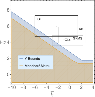
Figure 5: Comparison of our positivity bounds on $\bar{l}_{1}$ and $\bar{l}_{2}$ with those of Manohar and Mateu Manohar:2008tc for the $\pi\pi$ scattering to one loop. See Eqs. (25) to (30) for the error estimates for these bounds. The rectangles GL, ABT, GKMS and the small ellipse inside it are the ranges of the fitted values of $\bar{l}_{1}$ and $\bar{l}_{2}$ given in Refs. Gasser:1983yg , Girlanda:1997ed , Amoros:2000mc and Colangelo:2001df respectively.

4.3 Bounds on the $b_{i}$ constants

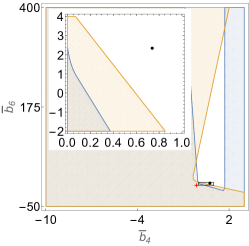
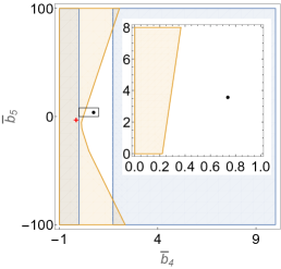
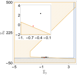
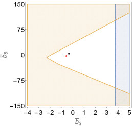
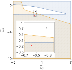
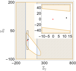
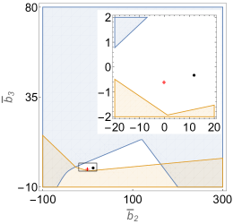
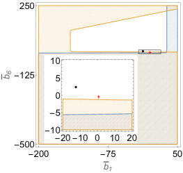
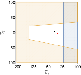
Figure 6: 2D sections of the constrained $b_{i}$ space. The 2D sections are obtained by setting the other $4$ parameters to the central values of the fit (33). The yellow (blue) region is the region ruled out by the bounds with $\eta=1$ ($\eta=0$). The black point represents the central values of the fit (33) with inputs from the experimental data and theoretical estimates, and the red cross represents the theoretical point computed from the Weinberg Lagrangian. To be continued in Fig 7.

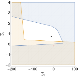
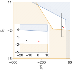
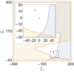
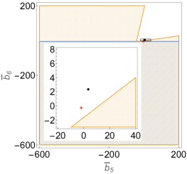
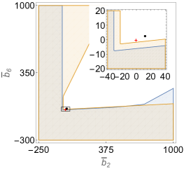
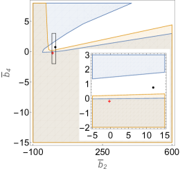
Figure 7: Continuation of Fig 6.

There are six $b_{i}$ constants ($i=1,2,...,6$) which appear linearly in the amplitude (5) and are functions of the $\mathcal{O}(p^{4})$ and $\mathcal{O}(p^{6})$ LECs. In this section, we shall apply the $Y$ positivity bounds on the two-loop ChPT amplitude to get the strongest bounds on the $b_{i}$ constants for different choices of $\{\eta,t,N,M\}$. Specifically, we will apply $1430$ $Y$ bounds with $\eta=0,1$, $N<6$, $M<11$ and $13$ values of $t$.

The $b_{i}$ constants contain powers of the $4\pi$ factor and are not naturally order one, so instead we will present results in terms of

$$\bar{b}_{i}\equiv(16\pi^{2})^{\zeta_{i}}b_{i},~{}~{}~{}~{}\zeta_{i}=1~{}{\rm for}~{}i=1,2,3,4,~{}~{}\zeta_{i}=2~{}{\rm for}~{}i=5,6.$$ (31)

The values of $\bar{b}_{i}$ from the $\mathcal{L}_{0}$ Weinberg Lagrangian with all the higher order LECs setting to zero up to two loops are given by

$${\bar{b}^{0}_{1}=\frac{13}{18},}~{}~{}{\bar{b}^{0}_{2}=-\frac{2}{9},}~{}~{}{\bar{b}^{0}_{3}=-\frac{7}{12},}~{}~{}{\bar{b}^{0}_{4}=-\frac{5}{36},}~{}~{}{\bar{b}^{0}_{5}=\frac{-66029+2688\pi^{2}}{20736},}~{}~{}{\bar{b}^{0}_{6}=\frac{-11375+768\pi^{2}}{20736}}.$$ (32)

This is, however, not a good approximation of the amplitude to that order, even not considering the fact that the LECs in the higher order Lagrangian are needed to absorb the UV divergence from the loop integrals. A good fit of these constants is provided by Colangelo et al. Colangelo:2001df

$$\begin{array}[]{lll}{\bar{b}_{1}=-12.4\pm 1.6,}&{\bar{b}_{2}=11.8\pm 0.6,}&{\bar{b}_{3}=-0.33\pm 0.07},\\ {\bar{b}_{4}=0.74\pm 0.01,}&{\bar{b}_{5}=3.58\pm 0.37,}&{\bar{b}_{6}=2.35\pm 0.02}.\end{array}$$ (33)

where the uncertainties come from higher order corrections in the EFT and from the experimental data input when solving the Roy equations.

The positivity bounds on ChPT carve out a geometric shape in 6D space $(b_{1},b_{2},b_{3},b_{4},b_{5},b_{6})$. It is clear that the constrained $b_{i}$ space has to be convex. This is simply because if two points $b_{i}$ and $b^{\prime}_{i}$ satisfy the positivity bounds $\sum_{i}a_{i}b_{i}>a_{0}$ and $\sum_{i}a_{i}b^{\prime}_{i}>a_{0}$, then any point in between the two points $b^{\prime\prime}_{i}={\lambda}b_{i}+(1-{\lambda})b^{\prime}_{i}$ also satisfies the positivity bounds. We cannot visualize a 6D constrained $b_{i}$ space, so we will look at the lower dimensional sections of the space with extra dimensions projected to the central values of the fit (33).

Let us look at the 2D projections of the constrained $b_{i}$ space (the 3D sections can be found in Appendix B). Setting the other $4$ parameters to the central values of the fit in Eq. (33), there are $15$ pairs of $\{\bar{b}_{i},\bar{b}_{j}\}$. We see from Figures 6 and 7 that for most of these sections of the constrained $b_{i}$ space (except for $\{\bar{b}_{5},\bar{b}_{6}\}$, $\{\bar{b}_{2},\bar{b}_{6}\}$, $\{\bar{b}_{2},\bar{b}_{4}\}$), the parameter space allowed by our positivity bounds are enclosed/compact regions. The boundary of the constrained $b_{i}$ space can be either straight lines or curly lines, the latter corresponding to choosing continuous values of $t$ in the positivity bounds. The black point represents the central value point of Eq. (33) and the red cross represents the parameters computed from the $\mathcal{L}_{0}$ Lagrangian with necessary counter terms. The $\mathcal{L}_{0}$ value is, not surprisingly, ruled out by our bounds in some sections, while the fit in Eq. (33) with its error bars are consistent with our positivity bounds. The constraints on the scale-independent coefficients $\bar{r}_{i}$ can be easily deduced from those on $b_{i}$ since they are linearly related to each other, see Appendix A.

5 Improved $Y$ bounds on ChPT

As discussed in Section 3.2, if the imaginary part of the amplitude can be accurately determined, one may subtract out the low energy contribution of the dispersion integral, and this will improve the positivity bounds.

5.1 Structure of the bounds

The dependence of the improved bounds on the parameters $\{\eta_{1},\eta_{2},t,N,M\}$ is very similar to that of the original $Y$ bounds. In particular, the improved dispersion relation is still $s\leftrightarrow u$ symmetric, so only $\eta=(\eta_{1}+\eta_{2})/2$ appears in the bounds linearly, and we only need to consider the bounds with $\eta=0$ and $1$. We need to consider different $t$ and only need to consider the low orders of $N$ and $M$. However, for improved bounds, we also have the parameter $\epsilon\Lambda$ to choose. A small $\epsilon\Lambda$ does not improve the bounds very much, while, to achieve a sufficient accuracy, $\epsilon\Lambda$ cannot be too close to $\Lambda$ ($\epsilon\Lambda=4$ corresponding to the original positivity bounds for which there is no subtraction of the imaginary part of the amplitude). The possible choice of $\epsilon\Lambda$ is clearly limited by how well the EFT at a given order can approximate the imaginary part of the full amplitude. Indeed, we find that the improved $Y$ bounds will break down at energies far below $\Lambda$ in ChPT. Assuming the current experimental determination of the $b_{i}$ constants are more or less accurate, this can be used to set a rough scale when the EFT at a given order stops being an effective description of the underlying physics. In Figure 8, we plot the distance in the $b_{i}$ space between the positivity plane and the fiducial point of $b_{i}$ given by the experimentally fitted values in (33). A negative distance in the plot indicates that the positivity plane has excluded the fiducial point, which implies that the improved positivity bound breaks down around that scale, as a valid positivity bound should not exclude the relatively good experimental values. We see that the first bound to become invalid is that of $N=2,M=1,2$ when $\epsilon\Lambda M_{\pi}\simeq 490{\rm MeV}$, with the other bounds also becoming negative at around $600{\rm MeV}$. Thus, we should not use the improved positivity bounds beyond $\epsilon\Lambda M_{\pi}\simeq 490{\rm MeV}$ and preferably somewhat below that scale. Nevertheless, a priori the exact scale $\epsilon\Lambda$ at which the improved positivity bounds lose their accuracy is difficult to pin down, so we shall present the results for different $\epsilon\Lambda M_{\pi}$ below $490{\rm MeV}$.

Physically, the limit of the choices of $\epsilon\Lambda$ is due to the onset of the scalar isoscalar resonance $f_{0}(500)$ (also known as the $\sigma$ meson), which couples to the $\pi\pi$ $S$ wave with isospin 0 and has a pole at $449^{+22}_{-16}-i(275\pm 12)$ MeV in the second Riemann sheet of the complex energy plane as determined from dispersive analyses Pelaez:2015qba . It is not included explicitly in ChPT, and a pole cannot be obtained with a perturbative momentum expansion to any finite order. Thus, perturbativity will break down at a scale where the $f_{0}(500)$ becomes important.

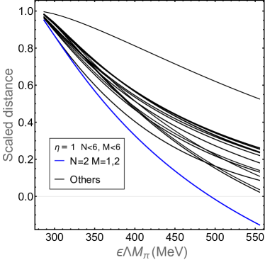
Figure 8: Distances between the improved bound planes and a fiducial point of $b_{i}$ (the central value of the empirically fitted values in Eq. (33)) in the $(b_{1},b_{2},b_{3},b_{4},b_{5},b_{6})$ space for $\eta=1$, $t=4$ at different energy scales. The distances are normalized to 1 at $\epsilon\Lambda=2$ (i.e., the original $Y$ bounds without improved subtractions) to facilitate visualization in the plot, and a negative distance indicates that the positivity plane has excluded the fiducial point. The $\{N=2,M=1,2\}$ bounds are the first bounds to become negative at $\epsilon\Lambda M_{\pi}\simeq 490{\rm MeV}$, beyond which the improved bounds become invalid.

Another thing one needs to consider in applying the improved bounds, actually somewhat related to what was discussed above, is that we need to check whether the perturbative expansion of the bounds themselves is respected. Let us see how this is supposed to work. At low energies, the usual EFT power counting suggests that $\tilde{B}_{\epsilon\Lambda}(v,t)$ be expanded as

$$B_{\epsilon\Lambda}(s,t)=\tilde{B}_{\epsilon\Lambda}(v,t)=B_{0}\sum_{i=0}^{\infty}\left(\frac{M_{\pi}^{2}}{\Lambda^{2}}\right)^{i}f^{\epsilon\Lambda}_{i}(v,t),$$ (34)

where $B_{0}$ is a dimensionless constant and $f^{\epsilon\Lambda}_{i}(v,t)$ is a dimensionless function of dimensionless variables $v$ and $t$. This expansion is valid when $f^{\epsilon\Lambda}_{i}(v,t)\sim v\sim t\sim 1$, as usually assumed. Plugging this into the improved $Y$ bounds, we get

$$\sum_{i=0}^{\infty}\left(\frac{M_{\pi}^{2}}{\Lambda^{2}}\right)^{i}Y_{\epsilon\Lambda,i}^{(2N,M)}(t)>0,$$ (35)

where $Y_{\epsilon\Lambda,i}^{(2N,M)}(t)$ is similar to $Y_{\epsilon\Lambda}^{(2N,M)}(t)$ with the replacement of $\tilde{B}_{\epsilon\Lambda}(v,t)$ with $f^{\epsilon\Lambda}_{i}(v,t)$. Assuming that higher order terms are smaller and truncating the expansion to a finite order, we get the positivity bounds for the EFT, and the truncation error may be estimated by the term after the truncation. For the original $Y$ bounds in ChPT, this perturbative structure is respected for a reasonably small ${M_{\pi}^{2}}/{\Lambda^{2}}$, where the two-loop contribution is smaller than the one-loop contribution. This, however, may not be so for the improved bounds with a large $\epsilon\Lambda$ subtraction. For an amplitude up to two loops, this can be verified, and we shall discard the bounds for which perturbativity is violated. Furthermore, even if perturbativity is respected for the expansion, at a practical level, it is also desirable that the improvements on the bounds gained by the $\epsilon\Lambda$ subtractions can outrun the extra uncertainties introduced by the subtractions per se.

5.2 Bounds on $\bar{l}_{1}$ and $\bar{l}_{2}$

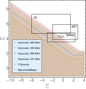
Figure 9: Improved $Y$ bounds on $\bar{l}_{1}$ and $\bar{l}_{2}$ for the $\pi\pi$ scattering to one loop for different $\epsilon\Lambda$ subtractions. For example, the red line is for $\epsilon\Lambda M_{\pi}=468~{}{\rm MeV}$. “Y bounds” indicates no $\epsilon\Lambda$ subtraction and “Manohar&Mateu” is the bounds from Manohar:2008tc . The rectangles GL, ABT, GKMS and the small ellipse inside it are the ranges of the fitted values of $\bar{l}_{1}$ and $\bar{l}_{2}$ given in Gasser:1983yg , Girlanda:1997ed , Amoros:2000mc and Colangelo:2001df respectively.

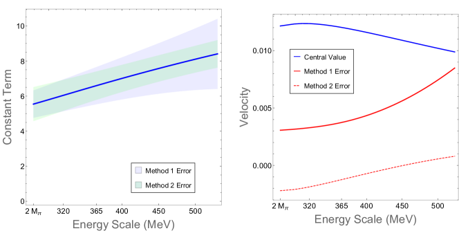
Figure 10: Error estimates of the improved $\bar{l}_{1}$ and $\bar{l}_{2}$ bounds for different $\epsilon\Lambda$ subtractions (“Energy Scale” denotes the value of $\epsilon\Lambda M_{\pi}$). The left subfigure shows the error estimates of the $\bar{l}_{2}+2\bar{l}_{2}$ bounds (“Constant Term” denotes the right hand side of $\bar{l}_{2}+2\bar{l}_{2}>{\rm Constant~{}Term}$, which depends on the $\epsilon\Lambda$ subtraction). The blue solid line is the $\mathcal{O}(p^{4})$ value of the Constant Term, and the error is estimated with the value of the Constant Term at $\mathcal{O}(p^{6})$. Two error estimation methods are represented: Method 1 (light blue region) is to only compute the two loop contribution at $\mathcal{O}(p^{6})$ and multiply it by a factor of 3, which is to roughly account for the badly known tree and one loop contributions at $\mathcal{O}(p^{6})$; Method 2 (light green region) is to set all the $b_{i}$ constants to the central values of their estimates provided by Colangelo et al. Colangelo:2001df at $\mathcal{O}(p^{6})$ (see Eq. (33)). The right subfigure shows the growth rate of the $\mathcal{O}(p^{4})$ value of the Constant Term (blue line, ”Central Value”) and the error estimates (red solid line for Method 1 and red dashed line for Method 2) for the left subfigure. We see that for $\epsilon\Lambda$ below $490$MeV the improvement of the bounds outruns the increase of the error estimates.

We first use the improved $Y$ bounds to constrain the LECs $\bar{l}_{1}$ and $\bar{l}_{2}$ at NLO. As mentioned above, we shall discard the improved bounds where perturbativity breaks down, for which we need to compare the $\mathcal{O}(p^{4})$ and $\mathcal{O}(p^{6})$ contributions. As mentioned above, improved positivity bounds become invalid when $\epsilon\Lambda M_{\pi}>490$ MeV. For improved subtractions below 490 MeV, we will further check whether the improvements on the constraints on $\bar{l}_{1}$ and $\bar{l}_{2}$ can outrun the errors introduced by the very subtraction procedure. While the constraints on $\bar{l}_{1}$ and $\bar{l}_{2}$ can be obtained with the $\mathcal{O}(p^{4})$ amplitude, we can estimate errors from the higher orders. As mentioned before, the LECs needed to evaluate the $\mathcal{O}(p^{6})$ amplitude are badly known. We will however use two different methods to estimate the errors: Method 1 is again to only compute the two loop contribution at $\mathcal{O}(p^{6})$ and multiply it by a factor of 3, to roughly account for the badly known tree and one loop contributions at $\mathcal{O}(p^{6})$; Method 2 is to set all the $b_{i}$ constants to the central values of their estimates provided by Colangelo et al. Colangelo:2001df at $\mathcal{O}(p^{6})$ (see Eq. (33)). As with Method 1, Method 2 is not a rigorous procedure either, but one can see in Figure 10 that the two methods are mostly consistent with each other. For the parameter space of $\bar{l}_{1}$ and $\bar{l}_{2}$, it is the improved $\bar{l}_{1}+2\bar{l}_{2}$ bounds that provide essential improvements on the constraints as compared to the original bounds. See Figure 10 for the error estimates of the improved $\bar{l}_{1}+2\bar{l}_{2}$ bounds for different $\epsilon\Lambda$ subtractions, which shows that the errors increase relatively slower than the improvements on the bounds. One can count a couple of reasons for this. First, in the construction of the improved $Y$ bounds, $\mathcal{M}^{2}$ is increased from $2+t/2$ to $\epsilon^{2}\Lambda^{2}+t/2-2$, which suppresses the errors as the improved $Y$ bounds contain various factors of $1/\mathcal{M}^{2}$. Also, the $\mathcal{O}(p^{6})$ contribution from the subtraction integral of the improved bound is much smaller than the $\mathcal{O}(p^{6})$ contribution from the original $B(s,t)$ amplitude, the former being less than $\sim 2\%$ of the later for $\epsilon\Lambda M_{\pi}$ up to 550MeV. Therefore, the improvements on the bounds gained by the $\epsilon\Lambda$ subtractions in this case appear to outrun the extra errors introduced by the subtractions (See the right subfigure of Figure 10).

To illustrate the results, we choose to look at 4 choices for $\epsilon\Lambda M_{\pi}$: 341 MeV, 388 MeV, 430 MeV and 468 MeV, and vary different $\{\eta,t,N,M\}$ to get the strongest bounds. Not surprisingly, the constraints are stronger for large $\epsilon\Lambda$; see Figure 9 for the results. For this particular case, the shape of the strongest bounds are unchanged after the $\epsilon\Lambda$ subtraction, and the improved bounds shift the bounds upwards.

Note that the improved bounds are also independent of the pion mass and decay constant at the one-loop level, and similar to the original $Y$ bounds, the bounds with $N>1$ give rise to trivial results. We have checked that the improved bounds $Y_{\epsilon\Lambda}^{(2N,M)}(t)={\rm const}>0$ are satisfied for $2\leq\epsilon\Lambda\leq 10$, $1<N<6,M<11$ and $13$ values of $t$.

5.3 Bounds on the $b_{i}$ constants

We also want to use the improved bounds to enhance the bounds on the $b_{i}$ constants. Again, we shall discard the improved bounds where perturbativity breaks down, and we choose to look at 4 choices for $\epsilon\Lambda M_{\pi}$: 341 MeV, 388 MeV, 430 MeV and 468 MeV, and vary different $\{\eta,t,N,M\}$ to get the strongest bounds. Similarly, we see that greater $\epsilon\Lambda$ leads to better constraints on $b_{i}$; see Figure 11 and 12.

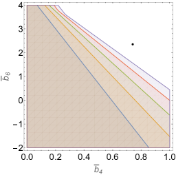
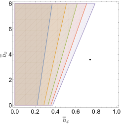
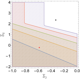
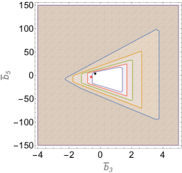
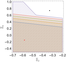
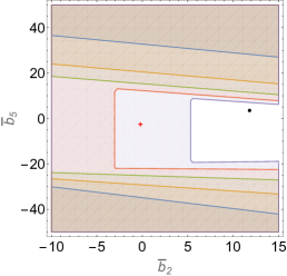
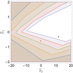
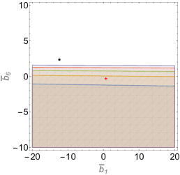
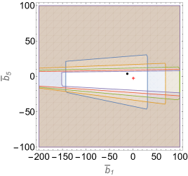
Figure 11: 2D sections of the improved constrained $b_{i}$ space. The 2D sections are obtained by setting the other $4$ parameters to the central values of the fit (33). The black point represents the central values of the fit (33) with inputs from the experimental data and theoretical estimates, and the red cross represents the theoretical point computed from the Weinberg Lagrangian. Different lines corresponds to different choices of $\epsilon\Lambda M_{\pi}$: $341$ MeV (Orange), $388$ MeV (green), $430$ MeV (Red), $468$ MeV (Purple), original $Y$ bounds (blue). To be continued in Figure 12.

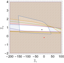
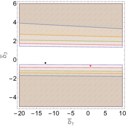
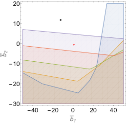
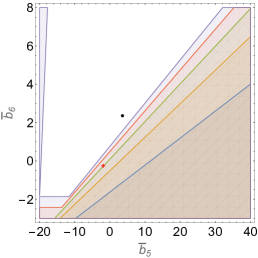
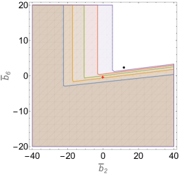
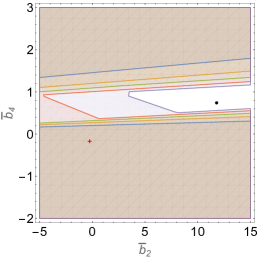
Figure 12: Continuation of Figure 11.

5.4 Padé approximation

Unitarity is only perturbatively respected in ChPT. It is well-known that the ChPT amplitude at leading orders violates unitarity at relatively low energy scales because of the existence of the $f_{0}(500)$ resonance. There are various methods to resum the ChPT scattering amplitudes in order to restore the exact unitarity Truong:1988zp ; Dobado:1989qm ; Truong:1991gv ; Dobado:1996ps ; Oller:1997ti ; Oller:1997ng ; Oller:1998hw ; Oller:1998zr ; Hannah:1999ev ; Nieves:1999bx ; Oller:2000fj ; Oller:2000ma ; GomezNicola:2001as ; Pelaez:2015qba (for works on unitarized ChPT at two loops, see Refs. Nieves:1999bx ; Pelaez:2006nj ); the meson-meson scattering data can be described in such nonperturbative approaches up to around 1.2 GeV, far higher than that of the perturbative ChPT. A very convenient and extensively used method to restore unitarity up to close to the cutoff scale is to make use of a mathematical tool, called Padé approximation Truong:1988zp ; Dobado:1989qm ; Dobado:1996ps ; Oller:1997ng ; Oller:1998hw ; Hannah:1999ev . We want to check whether the same trick can be applied to the improved positivity bounds.

In the Padé unitarization, the Padé approximation is applied to the partial waves of the isospin amplitude

$$T^{I}(s,t,u)=16\pi\sqrt{\frac{s}{s-4}}\sum_{\ell}(2\ell+1)P_{\ell}(\cos\theta)T_{I}^{\ell}(s).$$ (36)

In our case, the ChPT amplitude is calculated to two loops, $T_{{\ell}}^{I}(s)=T_{{\ell},1}^{I}(s)+T_{{\ell},2}^{I}(s)+T_{{\ell},3}^{I}(s)$ with subscripts 1,2,3 indicating the order of $x_{2}$, so we can take the [1,2] Padé approximation, which is to replace $T_{I}^{\ell}(s)$ with

$$T_{{\ell}}^{I[1,2]}(s)=\frac{T_{{\ell},1}^{I}(s)}{1-\frac{T_{{\ell},2}^{I}(s)}{T_{{\ell},1}^{I}(s)}-\frac{T_{{\ell},3}^{I}(s)}{T_{{\ell},1}^{I}(s)}+\left(\frac{T_{{\ell},2}^{I}(s)}{T_{{\ell},1}^{I}(s)}\right)^{2}}.$$ (37)

Since perturbative unitarity is satisfied order by order, we can show that the unitarized partial wave amplitude $T_{{\ell}}^{I[1,2]}(s)$ satisfies the unitarity relation $\operatorname{Im}T_{{\ell}}^{I[1,2]}(s)=\left|T_{{\ell}}^{I[1,2]}(s)\right|^{2}$, which is very useful in many circumstances (for reviews, see Refs. Oller:2000ma ; Pelaez:2015qba ; Oller:2019opk ).

However, we find that the unitarized Padé amplitude actually significantly lower the value of $\epsilon\Lambda$ that can be used to subtract the dispersion integral in the improved positivity bounds. In other words, in a sense, the Padé amplitude has worse dispersive properties than the original amplitude. For example, if we Padé unitarize the $\pi^{0}\pi^{0}\rightarrow\pi^{0}\pi^{0}$ amplitude, using it for the improved $Y$ bounds, and employ the same $b_{i}$ constants in Eq. (33), the energy scale $\epsilon\Lambda M_{\pi}$ at which the improved $t=1.1,N=2,M=8$ bound becomes negative is at $305$ MeV; see Figure 13. In comparison, using the original amplitude, the $t=1.1,N=2,M=2$ bound only breaks down after $500$ MeV. One need, however, to bear in mind that in principle the LECs in the unitarized amplitudes should take different values than those determined from the ChPT amplitude. For example, it was found previously for the scattering between the pseudo-Goldstone bosons and charmed mesons: the LECs determined from lattice QCD data using the unitarized ChPT in that case do not fulfill the positivity bounds derived for the perturbative amplitudes Du:2016tgp . In any case, the simple Padé unitarization procedure does not improve the analytic properties of the amplitude in terms of dispersion relations. Other undesirable properties of the Padé unitarization have been noticed previously, such as predicting spurious physical sheet resonances Ang:2001bd ; Qin:2002hk and incorrect coefficients for the leading chiral logarithms in higher loop diagrams Gasser:1990bv .

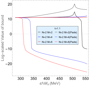
Figure 13: Comparison of the improved $Y$ bounds with (solid lines) and without (dashed lines) the Padé approximation. The example is for the $\pi^{0}\pi^{0}\rightarrow\pi^{0}\pi^{0}$ scattering amplitude up to two loops. The longitudinal axis indicates the logarithmically scaled values of the bounds.

6 Summary

We have applied the generalized positivity bounds (the $Y$ bounds and the improved $Y$ bounds) to ChPT to NNLO. This allows us to constrain the $\bar{l}_{i}$ LECs and the $b_{i}$ constants, which are combinations of LECs, to be within convex regions respectively. The constrained regions are convex because the $Y$ bounds produce inequalities that are linear in $\bar{l}_{i}$ and $b_{i}$. We see that constraints from the new bounds are stronger than the constraints obtained by the previous positivity bounds. For the $\bar{l}_{i}$ constants, although the values fitted from experimental data combined with other theoretical estimates are widely believed to be relatively accurate by now, the constraints from the positivity bounds are still interesting because of the cleanness in its assumptions, which are merely the fundamental principles of quantum field theory such as unitarity and analyticity. Also, the bounds we obtained for the $\bar{l}_{i}$ constants are independent of the pion mass and the pion decay constant, so these bounds apply to any ChPT with the same underlying symmetry, not just for the ChPT derived from QCD. For the bounds on the six $b_{i}$ constants, we see that most of its 2D sections near the empirically fitted central values are enclosed, with the constraints in some directions stronger than the others. Moreover, we have applied the improved positivity bounds to constrain the $\bar{l}_{i}$ and $b_{i}$ constants, which can further enhance the bounds.

Using the improved positivity, we can detect an energy scale at which ChPT as an EFT must break down. This is because when the $\epsilon\Lambda$ subtraction is set sufficiently high, the empirically fitted values of the LECs will be in conflict with the positivity bounds. For ChPT from QCD, this scale is around 490 MeV, consistent with the existence of the $f_{0}(500)$ resonance. A well-known method to “magically” restore unitarity is to apply the Padé approximant for the partial waves of the isospin amplitude. However, we find that the Padé method is rather unsatisfactory to restore the dispersion relation, as the improved bounds with the Padé unitarized amplitude actually break down at much lower energy scales.

Appendix A Loop functions and $b_{i}$ constants

Here we list the explicit expressions for the loop functions and the $b_{i}$ constants. The loop functions $F^{(i)}(s)$ and $G^{(i)}(s,t)$ are defined as follows Bijnens:1995yn

$$F^{(1)}(s) =\frac{1}{2}\overline{J}(s)\left(s^{2}-1\right),$$ (38)

$$G^{(1)}(s,t) =\frac{1}{6}\overline{J}(t)\left(14-4s-10t+st+2t^{2}\right),$$ (39)

$$F^{(2)}(s) =\overline{J}(s)\left\{\frac{1}{16\pi^{2}}\left(\frac{503}{108}s^{3}-\frac{929}{54}s^{2}+\frac{887}{27}s-\frac{140}{9}\right)+b_{1}(4s-3)+b_{2}\left(s^{2}+4s-4\right)\right.$$

$$~{}~{}~{}\left.+\frac{b_{3}}{3}\left(8s^{3}-21s^{2}+48s-32\right)+\frac{b_{4}}{3}\left(16s^{3}-71s^{2}+112s-48\right)\right\}$$

$$~{}~{}~{}+\frac{1}{18}K_{1}(s)\left\{20s^{3}-119s^{2}+210s-135-\frac{9}{16}\pi^{2}(s-4)\right\}$$

$$~{}~{}~{}+\frac{1}{32}K_{2}(s)\left\{s\pi^{2}-24\right\}+\frac{1}{9}K_{3}(s)\left\{3s^{2}-17s+9\right\},$$ (40)

$$G^{(2)}(s,t) =\overline{J}(t)\left\{\frac{1}{16\pi^{2}}\left[\frac{412}{27}-\frac{s}{54}\left(t^{2}+5t+159\right)-t\left(\frac{267}{216}t^{2}-\frac{727}{108}t+\frac{1571}{108}\right)\right]\right.$$

$$~{}~{}~{}+b_{1}(2-t)+\frac{b_{2}}{3}(t-4)(2t+s-5)-\frac{b_{3}}{6}(t-4)^{2}(3t+2s-8)$$

$$~{}~{}~{}\left.+\frac{b_{4}}{6}\left(2s(3t-4)(t-4)-32t+40t^{2}-11t^{3}\right)\right\}$$

$$~{}~{}~{}+\frac{1}{36}K_{1}(t)\left\{174+8s-10t^{3}+72t^{2}-185t-\frac{\pi^{2}}{16}(t-4)(3s-8)\right\}$$

$$~{}~{}~{}+\frac{1}{9}K_{2}(t)\left\{1+4s+\frac{\pi^{2}}{64}t(3s-8)\right\}$$

$$~{}~{}~{}+\frac{1}{9}K_{3}(t)\left\{1+3st-s+3t^{2}-9t\right\}+\frac{5}{3}K_{4}(t)\left\{4-2s-t\right\},$$ (41)

where the functions $\overline{J}$ and $K_{i}$ are given by

$$\left(\begin{array}[]{c}{\overline{J}}\\ {K_{1}}\\ {K_{2}}\\ {K_{3}}\end{array}\right) =\left(\begin{array}[]{cccc}{0}&{0}&{z}&{-4\bar{N}}\\ {0}&{z}&{0}&{0}\\ {0}&{z^{2}}&{0}&{8}\\ {\bar{N}zs^{-1}}&{0}&{\pi^{2}(\bar{N}s)^{-1}}&{\pi^{2}}\end{array}\right)\left(\begin{array}[]{c}{h^{3}}\\ {h^{2}}\\ {h}\\ {-\left(2\bar{N}^{2}\right)^{-1}}\end{array}\right),$$ (54)

$$K_{4} =\frac{1}{sz}\left(\frac{1}{2}K_{1}+\frac{1}{3}K_{3}+\frac{1}{\bar{N}}\overline{J}+\frac{\left(\pi^{2}-6\right)s}{12\bar{N}^{2}}\right),$$ (55)

with

$$h(s)=\frac{1}{\bar{N}\sqrt{z}}\ln\frac{\sqrt{z}-1}{\sqrt{z}+1}\quad,\quad z=1-\frac{4}{s},\quad\bar{N}=16\pi^{2}.$$ (56)

The constants $b_{1},b_{2},...,b_{6}$ are given by

$$b_{1} =8l_{1}^{r}+2l_{3}^{r}-2l_{4}^{r}+\frac{7}{6}L+\frac{1}{16\pi^{2}}\frac{13}{18}$$

$$~{}~{}~{}+x_{2}\left\{\frac{1}{16\pi^{2}}\left[\frac{56}{9}l_{1}^{r}+\frac{80}{9}l_{2}^{r}+15l_{3}^{r}+\frac{26}{9}l_{4}^{r}+\frac{47}{108}L-\frac{17}{216}+\frac{1}{16\pi^{2}}\frac{3509}{1296}\right]\right.$$

$$~{}~{}~{}\left.+\frac{1}{6}\left[4k_{1}+28k_{2}-6k_{3}+13k_{4}\right]+\left[32l_{1}^{r}+12l_{3}^{r}-5l_{4}^{r}\right]l_{4}^{r}-8l_{3}^{r2}+r_{1}^{r}\right\},$$ (57)

$$b_{2} =-8l_{1}^{r}+2l_{4}^{r}-\frac{2}{3}L-\frac{1}{16\pi^{2}}\frac{2}{9}$$

$$~{}~{}~{}+x_{2}\left\{\frac{1}{16\pi^{2}}\left[-24l_{1}^{r}-\frac{166}{9}l_{2}^{r}-18l_{3}^{r}-\frac{8}{9}l_{4}^{r}-\frac{203}{54}L+\frac{317}{3456}-\frac{1}{16\pi^{2}}\frac{1789}{432}\right]\right.$$

$$~{}~{}~{}\left.-\frac{1}{6}\left[54k_{1}+62k_{2}+15k_{3}+10k_{4}\right]-\left[32l_{1}^{r}+4l_{3}^{r}-5l_{4}^{r}\right]l_{4}^{r}+r_{2}^{r}\right\},$$ (58)

$$b_{3} =2l_{1}^{r}+\frac{1}{2}l_{2}^{r}-\frac{1}{2}L-\frac{1}{16\pi^{2}}\frac{7}{12}$$

$$~{}~{}~{}+x_{2}\left\{\frac{1}{16\pi^{2}}\left[\frac{178}{9}l_{1}^{r}+\frac{38}{3}l_{2}^{r}-\frac{7}{3}l_{4}^{r}-\frac{365}{216}L-\frac{311}{6912}+\frac{1}{16\pi^{2}}\frac{7063}{864}\right]\right.$$

$$~{}~{}~{}\left.+2\left[4l_{1}^{r}+l_{2}^{r}\right]l_{4}^{r}+\frac{1}{6}\left[38k_{1}+30k_{2}-3k_{4}\right]+r_{3}^{r}\right\},$$ (59)

$$b_{4} =\frac{1}{2}l_{2}^{r}-\frac{1}{6}L-\frac{1}{16\pi^{2}}\frac{5}{36}$$ (60)

$$~{}~{}~{}+x_{2}\left\{\frac{1}{16\pi^{2}}\left[\frac{10}{9}l_{1}^{r}+\frac{4}{9}l_{2}^{r}-\frac{5}{9}l_{4}^{r}+\frac{47}{216}L+\frac{17}{3456}+\frac{1}{16\pi^{2}}\frac{1655}{2592}\right]\right.$$

$$~{}~{}~{}\left.+2l_{2}^{r}l_{4}^{r}-\frac{1}{6}\left[k_{1}+4k_{2}+k_{4}\right]+r_{4}^{r}\right\},$$ (61)

$$b_{5} =\frac{1}{16\pi^{2}}\left[-\frac{31}{6}l_{1}^{r}-\frac{145}{36}l_{2}^{r}+\frac{625}{288}L+\frac{7}{864}-\frac{1}{16\pi^{2}}\frac{66029}{20736}\right]-\frac{21}{16}k_{1}-\frac{107}{96}k_{2}+r_{5}^{r},$$ (62)

$$b_{6} =\frac{1}{16\pi^{2}}\left[-\frac{7}{18}l_{1}^{r}-\frac{35}{36}l_{2}^{r}+\frac{257}{864}L+\frac{1}{432}-\frac{1}{16\pi^{2}}\frac{11375}{20736}\right]-\frac{5}{48}k_{1}-\frac{25}{96}k_{2}+r_{6}^{r},$$ (63)

where $L=\frac{1}{16\pi^{2}}\ln\frac{M_{\pi}^{2}}{\mu^{2}}$ and $k_{i}=\left(4r_{i}^{r}-\gamma_{i}L\right)L$ with $\gamma_{1}={1}/{3},~{}\gamma_{2}={2}/{3},~{}\gamma_{3}=-{1}/{2},~{}\gamma_{4}=2$. $r_{i}^{r}$ are linear combinations of $c_{i}^{r}$, the renormalized LECs of $\mathcal{L}_{6}$; see Ref. Bijnens:1999hw for the explicit relations. The scale dependence of $l^{r}_{i}(\mu)$ and $r_{i}^{r}(\mu)$ can be separated out as follows

$$l_{i}^{r}(\mu) =\frac{\gamma_{i}}{32\pi^{2}}\left(\bar{l}_{i}+\ln\frac{M_{\pi}^{2}}{\mu^{2}}\right),$$ (64)

$$r_{i}^{r}(\mu) =d^{(2)}_{i}\left(\ln\frac{M_{\pi}^{2}}{\mu^{2}}\right)^{2}+d^{(1)}_{i}\ln\frac{M_{\pi}^{2}}{\mu^{2}}+\bar{r}_{i},$$ (65)

where $\bar{l}_{i}$ and $\bar{r}_{i}$ are scale independent LECs and $d^{(1)}_{i}$ and $d^{(2)}_{i}$ are fixed by $\mu{\mathrm{d}b_{i}}/{\mathrm{d}\mu}=0$. With these, we can write $\bar{r}_{i}$ in the following form

$$\bar{r}_{i}=q_{i}\cdot b_{i}+h_{i},$$ (66)

where $q_{1}=q_{2}=q_{3}=q_{4}={1}/{x_{2}},~{}q_{5}=q_{6}=1$, and

$$h_{1} =\frac{\bar{l}_{3}{}^{2}}{512\pi^{4}}+\frac{5\bar{l}_{4}{}^{2}}{256\pi^{4}}+\frac{3\bar{l}_{4}\bar{l}_{3}}{256\pi^{4}}+\frac{15\bar{l}_{3}}{1024\pi^{4}}-\frac{7\bar{l}_{1}}{1728\pi^{4}}-\frac{5\bar{l}_{2}}{432\pi^{4}}-\frac{\bar{l}_{1}\bar{l}_{4}}{48\pi^{4}}-\frac{13\bar{l}_{4}}{1152\pi^{4}}+\frac{17}{3456\pi^{2}}-\frac{3509}{331776\pi^{4}}$$

$$~{}~{}~{}+\frac{1}{x_{2}}\left(-\frac{\bar{l}_{1}}{12\pi^{2}}+\frac{\bar{l}_{3}}{32\pi^{2}}+\frac{\bar{l}_{4}}{8\pi^{2}}-\frac{13}{288\pi^{2}}\right),$$ (67)

$$h_{2} =-\frac{5\bar{l}_{4}{}^{2}}{256\pi^{4}}+\frac{\bar{l}_{1}\bar{l}_{4}}{48\pi^{4}}-\frac{\bar{l}_{3}\bar{l}_{4}}{256\pi^{4}}+\frac{\bar{l}_{4}}{288\pi^{4}}+\frac{\bar{l}_{1}}{64\pi^{4}}+\frac{83\bar{l}_{2}}{3456\pi^{4}}-\frac{9\bar{l}_{3}}{512\pi^{4}}-\frac{317}{55296\pi^{2}}+\frac{1789}{110592\pi^{4}}$$

$$~{}~{}~{}+\frac{1}{x_{2}}\left(\frac{\bar{l}_{1}}{12\pi^{2}}-\frac{\bar{l}_{4}}{8\pi^{2}}+\frac{1}{72\pi^{2}}\right),$$ (68)

$$h_{3} =-\frac{\bar{l}_{4}\bar{l}_{1}}{192\pi^{4}}-\frac{89\bar{l}_{1}}{6912\pi^{4}}-\frac{19\bar{l}_{2}}{1152\pi^{4}}-\frac{\bar{l}_{2}\bar{l}_{4}}{384\pi^{4}}+\frac{7\bar{l}_{4}}{768\pi^{4}}+\frac{311}{110592\pi^{2}}-\frac{7063}{221184\pi^{4}}$$

$$~{}~{}~{}+\frac{1}{x_{2}}\left(-\frac{\bar{l}_{1}}{48\pi^{2}}-\frac{\bar{l}_{2}}{96\pi^{2}}+\frac{7}{192\pi^{2}}\right),$$ (69)

$$h_{4} =-\frac{5\bar{l}_{1}}{6912\pi^{4}}-\frac{\bar{l}_{2}}{1728\pi^{4}}-\frac{\bar{l}_{2}\bar{l}_{4}}{384\pi^{4}}+\frac{5\bar{l}_{4}}{2304\pi^{4}}-\frac{17}{55296\pi^{2}}-\frac{1655}{663552\pi^{4}}$$

$$~{}~{}~{}+\frac{1}{x_{2}}\left(\frac{5}{576\pi^{2}}-\frac{\bar{l}_{2}}{96\pi^{2}}\right),$$ (70)

$$h_{5} =\frac{31\bar{l}_{1}}{9216\pi^{4}}+\frac{145\bar{l}_{2}}{27648\pi^{4}}-\frac{7}{13824\pi^{2}}+\frac{66029}{5308416\pi^{4}},$$ (71)

$$h_{6} =\frac{7\bar{l}_{1}}{27648\pi^{4}}+\frac{35\bar{l}_{2}}{27648\pi^{4}}-\frac{1}{6912\pi^{2}}+\frac{11375}{5308416\pi^{4}}.$$ (72)

Appendix B 3D sections of the constrained $b_{i}$ space

Here we list the plots of the 3D sections of the constrained $b_{i}$ space for the original $Y$ bounds. The 3D sections are obtained by setting the three of the six $b_{i}$ parameters to the central values of the fit (33). See Figures 14 and 15.

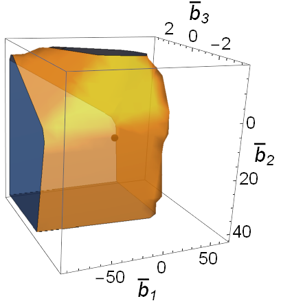
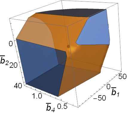
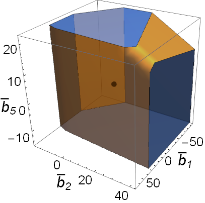
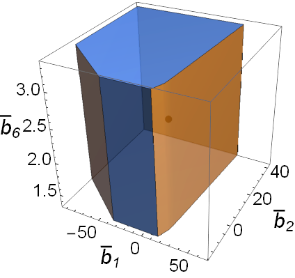
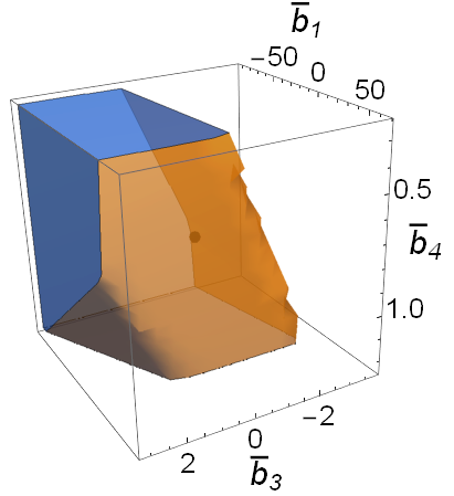
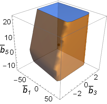
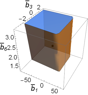
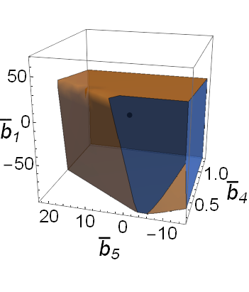
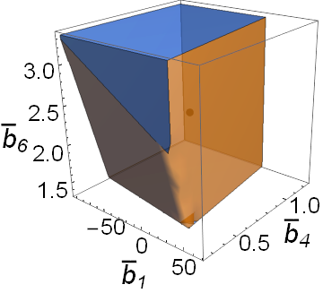
Figure 14: 3D sections of the constrained $b_{i}$ space. The 3D sections are obtained by setting the other $3$ parameters to the central values of the fit (33). The black point represents the central values of the fit (33) with inputs from the experimental data and theoretical estimates. To be continued in Figure 15.

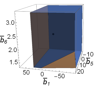
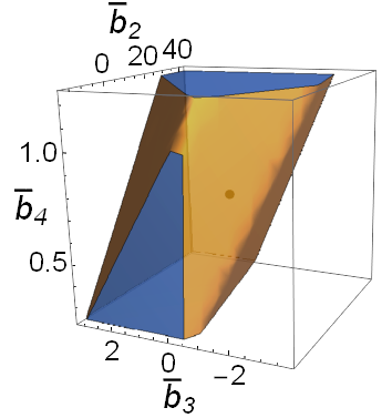
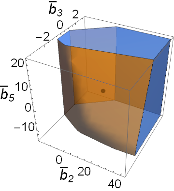
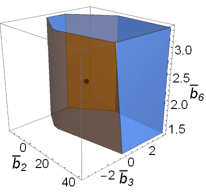
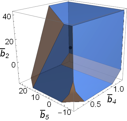
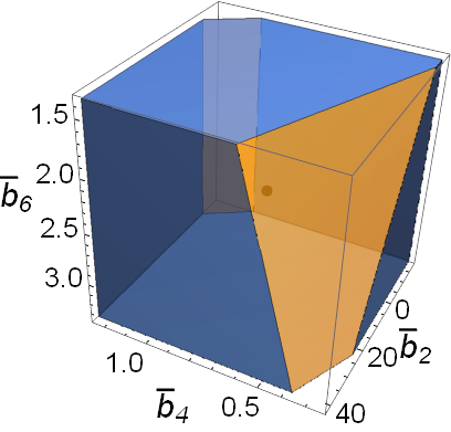
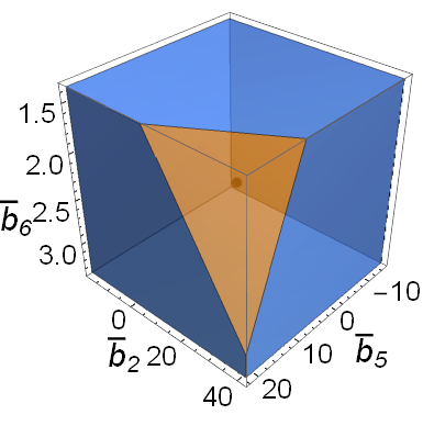
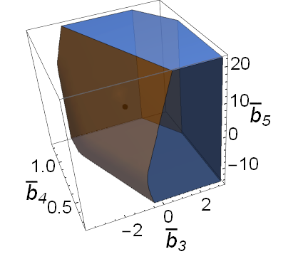
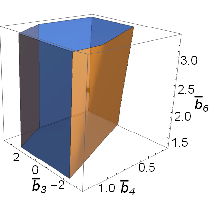
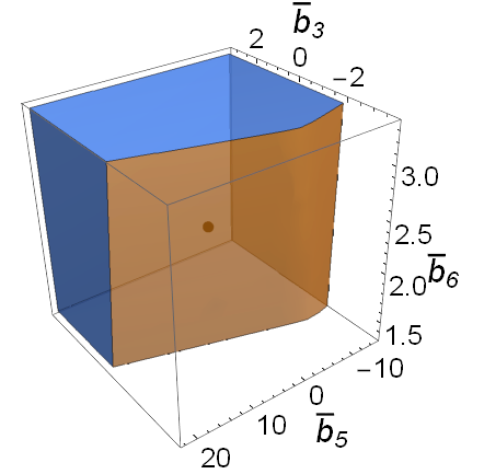
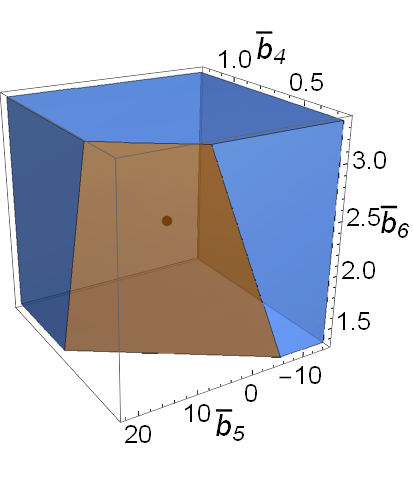
Figure 15: Continuation of Figure 14.

References

- (1) S. Weinberg, Pion scattering lengths, Phys. Rev. Lett. 17 (1966) 616–621.
- (2) L.-F. Li and H. Pagels, Perturbation theory about a Goldstone symmetry, Phys. Rev. Lett. 26 (1971) 1204–1206.
- (3) J. Gasser and H. Leutwyler, Chiral Perturbation Theory to One Loop, Annals Phys. 158 (1984) 142.
- (4) J. Gasser and H. Leutwyler, Chiral Perturbation Theory: Expansions in the Mass of the Strange Quark, Nucl. Phys. B250 (1985) 465–516.
- (5) A. Pich, Chiral perturbation theory, Rept. Prog. Phys. 58 (1995) 563–610, [hep-ph/9502366].
- (6) S. Scherer, Introduction to chiral perturbation theory, Adv. Nucl. Phys. 27 (2003) 277, [hep-ph/0210398].
- (7) V. Bernard and U.-G. Meißner, Chiral perturbation theory, Ann. Rev. Nucl. Part. Sci. 57 (2007) 33–60, [hep-ph/0611231].
- (8) S. R. Coleman, J. Wess and B. Zumino, Structure of phenomenological Lagrangians. 1., Phys. Rev. 177 (1969) 2239–2247.
- (9) C. G. Callan, Jr., S. R. Coleman, J. Wess and B. Zumino, Structure of phenomenological Lagrangians. 2., Phys. Rev. 177 (1969) 2247–2250.
- (10) A. Dobado, M. J. Herrero and J. Terron, The Role of Chiral Lagrangians in Strongly Interacting Signals at Supercolliders, Z. Phys. C50 (1991) 205–220.
- (11) J. Distler, B. Grinstein, R. A. Porto and I. Z. Rothstein, Falsifying Models of New Physics via WW Scattering, Phys. Rev. Lett. 98 (2007) 041601, [hep-ph/0604255].
- (12) T. N. Pham and T. N. Truong, Evaluation of the Derivative Quartic Terms of the Meson Chiral Lagrangian From Forward Dispersion Relation, Phys. Rev. D31 (1985) 3027.
- (13) M. R. Pennington and J. Portoles, The Chiral Lagrangian parameters, , , are determined by the resonance, Phys. Lett. B344 (1995) 399–406, [hep-ph/9409426].
- (14) B. Ananthanarayan, D. Toublan and G. Wanders, Consistency of the chiral pion pion scattering amplitudes with axiomatic constraints, Phys. Rev. D51 (1995) 1093–1100, [hep-ph/9410302].
- (15) J. Comellas, J. I. Latorre and J. Taron, Constraints on chiral perturbation theory parameters from QCD inequalities, Phys. Lett. B360 (1995) 109–116, [hep-ph/9507258].
- (16) P. Dita, Positivity constraints on chiral perturbation theory pion pion scattering amplitudes, Phys. Rev. D59 (1999) 094007, [hep-ph/9809568].
- (17) A. Adams, N. Arkani-Hamed, S. Dubovsky, A. Nicolis and R. Rattazzi, Causality, analyticity and an IR obstruction to UV completion, JHEP 10 (2006) 014, [hep-th/0602178].
- (18) A. V. Manohar and V. Mateu, Dispersion Relation Bounds for Scattering, Phys. Rev. D77 (2008) 094019, [0801.3222].
- (19) V. Mateu, Universal Bounds for SU(3) Low Energy Constants, Phys. Rev. D 77 (2008) 094020, [0801.3627].
- (20) A. Nicolis, R. Rattazzi and E. Trincherini, Energy’s and amplitudes’ positivity, JHEP 05 (2010) 095, [0912.4258].
- (21) B. Bellazzini, Softness and amplitudes’ positivity for spinning particles, JHEP 02 (2017) 034, [1605.06111].
- (22) C. de Rham, S. Melville, A. J. Tolley and S.-Y. Zhou, Positivity bounds for scalar field theories, Phys. Rev. D96 (2017) 081702, [1702.06134].
- (23) C. de Rham, S. Melville, A. J. Tolley and S.-Y. Zhou, UV complete me: Positivity Bounds for Particles with Spin, JHEP 03 (2018) 011, [1706.02712].
- (24) C. de Rham, S. Melville, A. J. Tolley and S.-Y. Zhou, Positivity Bounds for Massive Spin-1 and Spin-2 Fields, JHEP 03 (2019) 182, [1804.10624].
- (25) C. de Rham, S. Melville, A. J. Tolley and S.-Y. Zhou, Massive Galileon Positivity Bounds, JHEP 09 (2017) 072, [1702.08577].
- (26) C. Zhang and S.-Y. Zhou, Positivity bounds on vector boson scattering at the LHC, Phys. Rev. D100 (2019) 095003, [1808.00010].
- (27) Q. Bi, C. Zhang and S.-Y. Zhou, Positivity constraints on aQGC: carving out the physical parameter space, JHEP 06 (2019) 137, [1902.08977].
- (28) G. N. Remmen and N. L. Rodd, Consistency of the Standard Model Effective Field Theory, JHEP 12 (2019) 032, [1908.09845].
- (29) B. Bellazzini and F. Riva, New phenomenological and theoretical perspective on anomalous and processes, Phys. Rev. D98 (2018) 095021, [1806.09640].
- (30) D. Baumann, D. Green, H. Lee and R. A. Porto, Signs of Analyticity in Single-Field Inflation, Phys. Rev. D93 (2016) 023523, [1502.07304].
- (31) B. Bellazzini, C. Cheung and G. N. Remmen, Quantum Gravity Constraints from Unitarity and Analyticity, Phys. Rev. D93 (2016) 064076, [1509.00851].
- (32) C. Cheung and G. N. Remmen, Positive Signs in Massive Gravity, JHEP 04 (2016) 002, [1601.04068].
- (33) C. Cheung and G. N. Remmen, Positivity of Curvature-Squared Corrections in Gravity, Phys. Rev. Lett. 118 (2017) 051601, [1608.02942].
- (34) B. Bellazzini, F. Riva, J. Serra and F. Sgarlata, Beyond Positivity Bounds and the Fate of Massive Gravity, Phys. Rev. Lett. 120 (2018) 161101, [1710.02539].
- (35) J. Bonifacio, K. Hinterbichler and R. A. Rosen, Positivity constraints for pseudolinear massive spin-2 and vector Galileons, Phys. Rev. D94 (2016) 104001, [1607.06084].
- (36) K. Hinterbichler, A. Joyce and R. A. Rosen, Massive Spin-2 Scattering and Asymptotic Superluminality, JHEP 03 (2018) 051, [1708.05716].
- (37) J. Bonifacio, K. Hinterbichler, A. Joyce and R. A. Rosen, Massive and Massless Spin-2 Scattering and Asymptotic Superluminality, JHEP 06 (2018) 075, [1712.10020].
- (38) B. Bellazzini, F. Riva, J. Serra and F. Sgarlata, The other effective fermion compositeness, JHEP 11 (2017) 020, [1706.03070].
- (39) J. Bonifacio and K. Hinterbichler, Bounds on Amplitudes in Effective Theories with Massive Spinning Particles, Phys. Rev. D98 (2018) 045003, [1804.08686].
- (40) B. Bellazzini, M. Lewandowski and J. Serra, Positivity of Amplitudes, Weak Gravity Conjecture, and Modified Gravity, Phys. Rev. Lett. 123 (2019) 251103, [1902.03250].
- (41) S. Melville and J. Noller, Positivity in the Sky: Constraining dark energy and modified gravity from the UV, Phys. Rev. D101 (2020) 021502, [1904.05874].
- (42) C. de Rham and A. J. Tolley, The Speed of Gravity, 1909.00881.
- (43) L. Alberte, C. de Rham, A. Momeni, J. Rumbutis and A. J. Tolley, Positivity Constraints on Interacting Spin-2 Fields, 1910.11799.
- (44) L. Alberte, C. de Rham, A. Momeni, J. Rumbutis and A. J. Tolley, Positivity Constraints on Interacting Pseudo-Linear Spin-2 Fields, 1912.10018.
- (45) G. Ye and Y.-S. Piao, Positivity in the effective field theory of cosmological perturbations, 1908.08644.
- (46) M. Herrero-Valea, I. Timiryasov and A. Tokareva, To Positivity and Beyond, where Higgs-Dilaton Inflation has never gone before, 1905.08816.
- (47) J. J. Sanz-Cillero, D.-L. Yao and H.-Q. Zheng, Positivity constraints on the low-energy constants of the chiral pion-nucleon Lagrangian, Eur. Phys. J. C74 (2014) 2763, [1312.0664].
- (48) M.-L. Du, F.-K. Guo, U.-G. Meißner and D.-L. Yao, Aspects of the low-energy constants in the chiral Lagrangian for charmed mesons, Phys. Rev. D94 (2016) 094037, [1610.02963].
- (49) T. Appelquist and C. W. Bernard, Strongly Interacting Higgs Bosons, Phys. Rev. D22 (1980) 200.
- (50) A. C. Longhitano, Low-Energy Impact of a Heavy Higgs Boson Sector, Nucl. Phys. B188 (1981) 118–154.
- (51) A. C. Longhitano, Heavy Higgs Bosons in the Weinberg-Salam Model, Phys. Rev. D22 (1980) 1166.
- (52) M. J. Herrero and E. Ruiz Morales, The Electroweak chiral Lagrangian for the Standard Model with a heavy Higgs, Nucl. Phys. B418 (1994) 431–455, [hep-ph/9308276].
- (53) G. Buchalla and O. Cata, Effective Theory of a Dynamically Broken Electroweak Standard Model at NLO, JHEP 07 (2012) 101, [1203.6510].
- (54) G. Buchalla, O. Catà and C. Krause, Complete Electroweak Chiral Lagrangian with a Light Higgs at NLO, Nucl. Phys. B880 (2014) 552–573, [1307.5017].
- (55) R. Alonso, M. B. Gavela, L. Merlo, S. Rigolin and J. Yepes, The Effective Chiral Lagrangian for a Light Dynamical “Higgs Particle”, Phys. Lett. B722 (2013) 330–335, [1212.3305].
- (56) F.-K. Guo, P. Ruiz-Femenia and J. J. Sanz-Cillero, One loop renormalization of the electroweak chiral Lagrangian with a light Higgs boson, Phys. Rev. D92 (2015) 074005, [1506.04204].
- (57) G. Buchalla, O. Cata, A. Celis, M. Knecht and C. Krause, Complete One-Loop Renormalization of the Higgs-Electroweak Chiral Lagrangian, Nucl. Phys. B928 (2018) 93–106, [1710.06412].
- (58) R. Alonso, K. Kanshin and S. Saa, Renormalization group evolution of Higgs effective field theory, Phys. Rev. D97 (2018) 035010, [1710.06848].
- (59) E. E. Jenkins, A. V. Manohar and P. Stoffer, Low-Energy Effective Field Theory below the Electroweak Scale: Anomalous Dimensions, JHEP 01 (2018) 084, [1711.05270].
- (60) A. Pich, Effective Field Theory with Nambu-Goldstone Modes, in Les Houches summer school: EFT in Particle Physics and Cosmology Les Houches, Chamonix Valley, France, July 3-28, 2017, 2018. 1804.05664.
- (61) J. Bijnens, G. Colangelo, G. Ecker, J. Gasser and M. E. Sainio, Pion-pion scattering at low energy, Nucl. Phys. B508 (1997) 263–310, [hep-ph/9707291].
- (62) J. Bijnens, G. Colangelo and G. Ecker, The Mesonic chiral Lagrangian of order , JHEP 02 (1999) 020, [hep-ph/9902437].
- (63) J. Bijnens, G. Colangelo, G. Ecker, J. Gasser and M. E. Sainio, Elastic scattering to two loops, Phys. Lett. B374 (1996) 210–216, [hep-ph/9511397].
- (64) Particle Data Group collaboration, M. Tanabashi et al., Review of Particle Physics, Phys. Rev. D98 (2018) 030001.
- (65) A. Manohar and H. Georgi, Chiral Quarks and the Nonrelativistic Quark Model, Nucl. Phys. B234 (1984) 189–212.
- (66) M. Froissart, Asymptotic behavior and subtractions in the Mandelstam representation, Phys. Rev. 123 (1961) 1053–1057.
- (67) A. Martin, Unitarity and high-energy behavior of scattering amplitudes, Phys. Rev. 129 (1963) 1432–1436.
- (68) Y. S. Jin and A. Martin, Number of Subtractions in Fixed-Transfer Dispersion Relations, Phys. Rev. 135 (1964) B1375–B1377.
- (69) A. Martin, Extension of the axiomatic analyticity domain of scattering amplitudes by unitarity. 1., Nuovo Cim. A42 (1965) 930–953.
- (70) C. de Rham, S. Melville and A. J. Tolley, Improved Positivity Bounds and Massive Gravity, JHEP 04 (2018) 083, [1710.09611].
- (71) G. Colangelo, J. Gasser and H. Leutwyler, scattering, Nucl. Phys. B603 (2001) 125–179, [hep-ph/0103088].
- (72) L. Girlanda, M. Knecht, B. Moussallam and J. Stern, Comment on the prediction of two loop standard chiral perturbation theory for low-energy scattering, Phys. Lett. B409 (1997) 461–468, [hep-ph/9703448].
- (73) G. Amoros, J. Bijnens and P. Talavera, form-factors and - scattering, Nucl. Phys. B585 (2000) 293–352, [hep-ph/0003258].
- (74) J. R. Peláez, From controversy to precision on the sigma meson: a review on the status of the non-ordinary resonance, Phys. Rept. 658 (2016) 1, [1510.00653].
- (75) T. N. Truong, Chiral Perturbation Theory and Final State Theorem, Phys. Rev. Lett. 61 (1988) 2526.
- (76) A. Dobado, M. J. Herrero and T. N. Truong, Unitarized Chiral Perturbation Theory for Elastic Pion-Pion Scattering, Phys. Lett. B235 (1990) 134–140.
- (77) T. N. Truong, Remarks on the unitarization methods, Phys. Rev. Lett. 67 (1991) 2260–2263.
- (78) A. Dobado and J. R. Peláez, The Inverse amplitude method in chiral perturbation theory, Phys. Rev. D56 (1997) 3057–3073, [hep-ph/9604416].
- (79) J. A. Oller and E. Oset, Chiral symmetry amplitudes in the wave isoscalar and isovector channels and the , , scalar mesons, Nucl. Phys. A620 (1997) 438–456, [hep-ph/9702314].
- (80) J. A. Oller, E. Oset and J. R. Peláez, Nonperturbative approach to effective chiral Lagrangians and meson interactions, Phys. Rev. Lett. 80 (1998) 3452–3455, [hep-ph/9803242].
- (81) J. A. Oller, E. Oset and J. R. Peláez, Meson meson interaction in a nonperturbative chiral approach, Phys. Rev. D59 (1999) 074001, [hep-ph/9804209].
- (82) J. A. Oller and E. Oset, N/D description of two meson amplitudes and chiral symmetry, Phys. Rev. D60 (1999) 074023, [hep-ph/9809337].
- (83) T. Hannah, Pion scalar form-factor and the sigma meson, Phys. Rev. D60 (1999) 017502, [hep-ph/9905236].
- (84) J. Nieves and E. Ruiz Arriola, Bethe-Salpeter approach for unitarized chiral perturbation theory, Nucl. Phys. A679 (2000) 57–117, [hep-ph/9907469].
- (85) J. A. Oller and U.-G. Meißner, Chiral dynamics in the presence of bound states: Kaon nucleon interactions revisited, Phys. Lett. B500 (2001) 263–272, [hep-ph/0011146].
- (86) J. A. Oller, E. Oset and A. Ramos, Chiral unitary approach to meson meson and meson-baryon interactions and nuclear applications, Prog. Part. Nucl. Phys. 45 (2000) 157–242, [hep-ph/0002193].
- (87) A. Gomez Nicola and J. R. Pelaez, Meson meson scattering within one loop chiral perturbation theory and its unitarization, Phys. Rev. D65 (2002) 054009, [hep-ph/0109056].
- (88) J. R. Peláez and G. Rios, Nature of the from its dependence at two loops in unitarized Chiral Perturbation Theory, Phys. Rev. Lett. 97 (2006) 242002, [hep-ph/0610397].
- (89) J. A. Oller, Coupled-channel approach in hadron-hadron scattering, Prog. Part. Nucl. Phys. 110 (2020) 103728, [1909.00370].
- (90) Q. Ang, Z. Xiao, H. Zheng and X. C. Song, A Critical examination to the unitarized scattering chiral amplitudes, Commun. Theor. Phys. 36 (2001) 563–568, [hep-ph/0109012].
- (91) G.-Y. Qin, W. Z. Deng, Z. Xiao and H. Q. Zheng, The [1,2] Padé amplitudes for scatterings in chiral perturbation theory, Phys. Lett. B542 (2002) 89–99, [hep-ph/0205214].
- (92) J. Gasser and U. G. Meissner, Chiral expansion of pion form-factors beyond one loop, Nucl. Phys. B357 (1991) 90–128.
- (93) J. Bijnens, G. Colangelo and G. Ecker, Renormalization of chiral perturbation theory to order , Annals Phys. 280 (2000) 100–139, [hep-ph/9907333].