The general theory of permutation equivarant neural networks and higher order graph variational encoders

The general theory of permutation equivarant neural networks and higher order graph variational encoders

Abstract

Previous work on symmetric group equivariant neural networks generally only considered the case where the group acts by permuting the elements of a single vector. In this paper we derive formulae for general permutation equivariant layers, including the case where the layer acts on matrices by permuting their rows and columns simultaneously. This case arises naturally in graph learning and relation learning applications. As a specific case of higher order permutation equivariant networks, we present a second order graph variational encoder, and show that the latent distribution of equivariant generative models must be exchangeable. We demonstrate the efficacy of this architecture on the tasks of link prediction in citation graphs and molecular graph generation.

8pt SE[DOWHILE]DodoWhiledo[1]while #1

1 Introduction

Generalizing from the success of convolutional neural networks in computer vision, equivariance has emerged as a core organzing principle of deep neural network architectures. Classical CNNs are equivariant to translations (LeCun et al., 1989). In recent years, starting with (Cohen & Welling, 2016), researchers have also constructed networks that are equivariant to the three dimensional rotation group (CohenSpherical2018) (Kondor et al., 2018a), the Euclidean group of translations and rotations (Cohen & Welling, 2017)(Weiler et al., 2018), and other symmetry groups (Ravanbakhsh et al., 2017). Closely related are generalizations of convolution to manifolds (Marcos et al., 2017)(Worrall et al., 2017). Gauge equivariant CNNs form an overarching framework that connects the two domains (Cohen et al., 2019a).

The set of all permutations of $n$ objects also forms a group, called the symmetric group of degree $n$, commonly denoted ${\mathbb{S}_{n}}$. The concept of permutation equivariant neural networks was proposed in (Guttenberg et al., 2016), and discussed in depth in “Deep sets” by (Zaheer et al., 2017). Since then, permutation equivariant models have found applications in a number of domains, including understanding the compositional structure of language (Gordon et al., 2020), and such models were analyzed from theoretical point of view in (Keriven & Peyré, 2019) (Sannai et al., 2019). The common feature of all of these approaches however is that they only consider one specific way that permutations can act on vectors, namely $\smash{(f_{1},\ldots,f_{n})\mapsto(f_{\sigma^{-1}(1)},\ldots,f_{\sigma^{-1}(n)})}$. This is not sufficient to describe certain naturally occurring situations, for example, when ${\mathbb{S}_{n}}$ permutes the rows and columns of an adjacency matrix.

In the present paper we generalize the notion of permutation equivariant neural networks to other actions of the symmetric group, and derive the explicit form of the corresponding equivariant layers, including how many learnable parameters they can have. In this sense our paper is similar to recent works such as (Cohen et al., 2019b; Kondor & Trivedi, 2018; Yarotsky, 2018) which examined the algebric aspects of equivariant nets, but with a specific focus on the symmetric group.

On the practical side, higher order permutation equivariant neural networks appear naturally in graph learning and graph generation (Maron et al., 2019; Hy et al., 2018). More generally, we argue that this symmetry is critical for encoding relations between pairs, triples, quadruples etc. of entities rather than just whether a given object is a member of a set or not. As a specific example of our framework we present a second order equivariant graph variational encoder and demonstrate its use on link preduction and graph generation tasks. The distribution on the latent layer of such a model must be exchangeable (but not necessarily IID), forming and interesting connection to Bayesian nonparametric models (Bloem-Reddy & Teh, 2019).

2 Equivariance to permutations

A permutation (of order $n$) is a bijective map $\sigma\colon\{1,2,\ldots,n\}\to\{1,2,\ldots,n\}$. The product of one permutation $\sigma_{1}$ with another permutation $\sigma_{2}$ is the permutation that we get by first performing $\sigma_{1}$, then $\sigma_{2}$, i.e., $(\sigma_{2}\sigma_{1})(i):=\sigma_{2}(\sigma_{1}(i))$. It is easy to see that with respect to this notion of product, the set of all $n!$ permutations of order $n$ form a group. This group is called the symmetric group of degree $n$, and denoted ${\mathbb{S}_{n}}$.

Now consider a feed-forward neural network consisting of $s$ neurons, $\mathfrak{n}_{1},\mathfrak{n}_{2},\ldots,\mathfrak{n}_{s}$. We will denote the activation of the $i$’th neuron $f^{i}$. Each activation may be a scalar, a vector, a matrix or a tensor. As usual, we assume that the input to our network is a fixed size vector/matrix/tensor $x$, and the ouput is a fixed sized vector/matrix/tensor $y$.

The focus of the present paper is to study the behavior of neural networks under the action of ${\mathbb{S}_{n}}$ on the input $x$. This encompasses a range of special cases, relevant to different applications:

1. Trivial action. The simplest case is when ${\mathbb{S}_{n}}$ acts on $x$ trivially, i.e., $\sigma(x)=x$, so permutations don’t change $x$ at all. This case is not very interesting for our purposes.

2. First order permutation action. The simplest non-trivial ${\mathbb{S}_{n}}$–action is when $x$ is an $n$ dimensional vector and ${\mathbb{S}_{n}}$ permutes its elements:

   $$[\sigma(x)]_{i}=x_{\sigma^{-1}(i)}.$$ (1)

   This is the case that was investigated in (Zaheer et al., 2017) because it arises naturally when learning from sets, in particular when $x_{i}$ relates to the $i$’th element of a set $S$ of $n$ objects $\{o_{1},\ldots,o_{n}\}$. Permuting the numbering of the objects does not change $S$ as a set, but it does change the ordering of the elements of $x$ exactly as in (1). When learning from sets the goal is to construct a network which, as a whole, is invariant to the permutation action. A natural extension allowing us to describe each object with more than just a single number is when $x$ is an $n\times d$ dimensional matrix on which ${\mathbb{S}_{n}}$ acts by permuting its rows, $[\sigma(x)]_{i,j}=x_{\sigma^{-1}(i),\,j}$.

3. Second order permutation action. The second level in the hierarchy of permutation actions is the case when $x$ is an $n\times n$ matrix on which the symmetric group acts by permuting both its rows and its columns:

   $$[\sigma(x)]_{i,j}=x_{\sigma^{-1}(i),\,\sigma^{-1}(j)}.$$

   While this might look exotic at first sight, it is exactly the case faced by graph neural networks, where $x$ is the adjacency matrix of a graph. More generally, this case encompasses any situation involving learning from binary relations on a set.

4. Higher order cases. Extending the above, if $x$ is a tensor of order $k$, the $k$’th order permutation action of ${\mathbb{S}_{n}}$ on $x$ transforms it as

   $$[\sigma(x)]_{i_{1},\ldots,i_{k}}=x_{\sigma^{-1}(i_{1}),\ldots,\sigma^{-1}(i_{k})}.$$ (2)

   This case arises, for example, in problems involving rankings, and was also investigated in (Maron et al., 2019).

5. Other actions. Not all actions of ${\mathbb{S}_{n}}$ can be reduced to actually permuting the elements of a tensor. We will discuss more general cases in Section 4.

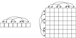
Figure 1: The symmetric group acts on vectors by permuting their elements (left). However, in this paper we also consider equivariance to other types of ${\mathbb{S}_{n}}$–actions, such as the way that a single permutation $\sigma\in{\mathbb{S}_{n}}$ permutes the rows and columns of an adjacency matrix simultaneously (right). The most general types of ${\mathbb{S}_{n}}$–actions are best expressed in Fourier space.

2.1 Invariance vs. equivariance

Neural networks learning from sets or graphs must be invariant to the action of the symmetric group on their inputs. However, even when a network is overall invariant, its internal activations are often expected to be equivariant (covariant) rather than invariant. In graph neural networks, for example, the output of the $\ell$’th layer is often a matrix $\smash{f^{\ell}}$ whose rows are indexed by the vertices (Bruna et al., 2014). If we permute the vertices, $\smash{f^{\ell}}$ will to change to $f^{\ell}\prime$, where $\smash{[f^{\ell}\prime]_{i,j}=[f^{\ell}]_{\sigma^{-1}(i),\,j}}$. It is only at the top of the network that invariance is enforced, typically by summing over the $i$ index of the penultimate layer.

Other applications demand that the output of the network be covariant with the permutation action. Consider, for example the case of learning to fill in the missing edges of a graph of $n$ vertices. In this case both the inputs and the outputs of the network are $n\times n$ adjacency matrices, so the output must transform according to the same action as the input. Naturally, the internal nodes of such a network must also co-vary with permutations. action on the inputs and cannot just be invariant.

In this paper we assume that every activation of the network covaries with permutations. However, each $f^{i}$ may transform according to a different action of the symmetric group. The general term for how these activations transform in a coordinated way is equivariance, which we define formally below. Note that invariance is a special case of equivariance corresponding to the trivial ${\mathbb{S}_{n}}$–action $\smash{\sigma(f^{i})=f^{i}}$. Finally, we note that in this paper we use the terms covariant and equivariant essentially interchangeably: in general, the former is more commonly used in the context of compositional architectures, whereas the latter is the generic term used for convolutional nets.

2.2 General definition of permutation equivariance

To keep our discussion as general as possible, we start with a general definition of symmetric group actions.

Definition 1.

Let $f$ be a vector, matrix or tensor representing the input to a neural network or the activation of one of its neurons. We say that the symmetric group ${\mathbb{S}_{n}}$ acts linearly on $f$ if under a permutation $\sigma\in{\mathbb{S}_{n}}$, $f$ changes to $T_{\sigma}(f)$ for some fixed collection of linear maps $\smash{\{\hskip 1.00006pt{T_{\sigma}}\>|\>{\sigma\in{\mathbb{S}_{n}}\hskip 1.00006pt}\}}$.

This definition is more general than the first, second and $k$’th order permutation actions described above, because it does not constrain $T_{\sigma}$ to just permute the entries of $f$. Rather, $T_{\sigma}$ can be any linear map. Our general notion of permutation equivariant networks is then the following.

Definition 2.

Let $\mathcal{N}$ be a neural network whose input is $x$ and whose activations are $f^{1},f^{2},\ldots f^{s}$. Assume that the symmetric group ${\mathbb{S}_{n}}$ acts on $x$ linearly by the maps $\smash{\{\hskip 1.00006pt{T^{\textrm{in}}_{\sigma}}\>|\>{\sigma\in{\mathbb{S}_{n}}\hskip 1.00006pt}\}}$. We say that $\mathcal{N}$ is equivariant to permutations if each of its neurons has a corresponding ${\mathbb{S}_{n}}$–action $\smash{\{\hskip 1.00006pt{T^{i}_{\sigma}}\>|\>{\sigma\in{\mathbb{S}_{n}}\hskip 1.00006pt}\}}$ such that when $x\mapsto T^{\textrm{in}}_{\sigma}(x)$,  $f^{i}$ will correspondingly transform as $\smash{f^{i}\mapsto T^{i}_{\sigma}(f^{i})}$.

Note that (Zaheer et al., 2017) only considered the case of first order permutation actions

$$(f^{i}_{1},\ldots,f^{i}_{n})\overset{\sigma}{\longmapsto}(f^{i}_{\sigma^{-1}(1)},\ldots,f^{i}_{\sigma^{-1}(n)}),$$ (3)

whereas our definition also covers richer forms of equivariance, including the second order case

$$(f^{i}_{1,1},f^{i}_{1,2},\ldots,f^{i}_{n,n})\overset{\sigma}{\longmapsto}\\ (f^{i}_{\sigma^{-1}(1),\sigma^{-1}(1)},f^{i}_{\sigma^{-1}(1),\sigma^{-1}(2)},\ldots,f^{i}_{\sigma^{-1}(n),\sigma^{-1}(n)})$$ (4)

that is relevant to graph and learning relation learning.

3 Convolutional architectures

Classical convolutional networks and their generalizations to groups are characterized by the following three features:

1. The neurons of the network are organized into distinct layers $\ell=0,1,\ldots L$. We will use $f^{\ell}$ to collectively denote the activations of all the neurons in layer $\ell$.

2. The output of layer $\ell$ can be expressed as

   $$f^{\ell}=\xi_{\ell}(\phi_{\ell}(f^{\ell-1})),$$

   where $\phi_{\ell}$ is a learnable linear function, while $\xi_{\ell}$ is a fixed nonlinearity.

3. The entire network is equivariant to the action of a global symmetry group $G$ in the sense that each $f_{\ell}$ has a corresponding $G$–action that is equivariant to the action of $G$ on the inputs.

Generalized convolutional networks have found applications in a wide range of domains and their properties have been thoroughly investigated (Cohen & Welling, 2016) (Ravanbakhsh et al., 2017) (Cohen et al., 2019b).

Kondor & Trivedi (2018) proved that in any neural network that follows the above axioms, the linear operation $\phi_{\ell}$ must be a generalized form of covolution, as long as $f^{\ell-1}$ and $f^{\ell}$ can be conceived of as functions on quotient spaces $G/H_{\ell-1}$ and $G/H_{\ell}$ with associated actions

$$\mathfrak{f}\overset{g}{\longmapsto}\mathfrak{f}^{g}\qquad\quad\mathfrak{f}^{g}(u)=\mathfrak{f}(g^{-1}u).$$

In this section we show that this result can be used to derive the most general form of convolutional networks whose activations transform according to $k$’th order permutation actions. Our key tools are Propositions 1–3 in the Appendix, which show that the quotient spaces corresponding to the first, second and $k$’th order permutation actions are ${\mathbb{S}_{n}}/\mathbb{S}_{n-1}$, ${\mathbb{S}_{n}}/\mathbb{S}_{n-2}$ and ${\mathbb{S}_{n}}/\mathbb{S}_{n-k}$:

1. First order action. If $f\in\mathbb{R}^{d}$ is a vector transforming as $f\overset{\sigma}{\longmapsto}f^{\sigma}$ with $f^{\sigma}=(f_{\sigma^{-1}(1)},\ldots,f_{\sigma^{-1}(n)})$, then the corresponding quotient space function is

   $$\mathfrak{f}(\mu)=f_{\mu(n)}\qquad\quad\qquad\quad\mu\in{\mathbb{S}_{n}}/\mathbb{S}_{n-1}.$$

2. Second order action. If $f\in\mathbb{R}^{n\times n}$ is a matrix with zero diagonal transforming as $f\overset{\sigma}{\longmapsto}f^{\sigma}$ where $f^{\sigma}_{i,j}=f_{\sigma^{-1}(i),\hskip 0.70004pt\sigma^{-1}(j)}$,  then the corresponding quotient space function is

   $$\mathfrak{f}(\mu)=f_{\mu(n),\,\mu(n-1)}\qquad\quad\mu\in{\mathbb{S}_{n}}/\mathbb{S}_{n-2}.$$

3. k’th order action. Let $f\in\mathbb{R}^{n\times\ldots\times n}$ be a $k$’th order tensor such that $f_{i_{1},\ldots,i_{k}}=0$ unless $i_{1},\ldots,i_{k}$ are all distinct. If $f$ transforms under permutations as $\smash{f\overset{\sigma}{\longmapsto}f^{\sigma}}$ where $\smash{f^{\sigma}_{i_{1},\ldots,i_{k}}=f_{\sigma^{-1}(i_{1}),\ldots,\sigma^{-1}(i_{k})}}$, then the corresponding quotient space function is

   $$\mathfrak{f}(\mu)=f_{\mu(n),\ldots,\mu(n-k+1)}\qquad\quad\mu\in{\mathbb{S}_{n}}/\mathbb{S}_{n-k}.$$

Theorem 1 of (Kondor & Trivedi, 2018) states that if the equivariant activations $f^{\ell-1}$ and $f^{\ell}$ both correspond to the same quotient space $S$, then the linear operation $\phi_{\ell}$ must be of the form

$$\phi_{\ell}(\mathfrak{f}_{\ell-1})=\mathfrak{f}_{\ell-1}\ast h_{\ell},$$

where $\ast$ denotes convolution on ${\mathbb{S}_{n}}$, and $h_{\ell}$ is a function $S\backslash{\mathbb{S}_{n}}/S\to\mathbb{R}$. Mapping $\phi(\mathfrak{f}_{\ell-1})$ back to the original vector/matrix/tensor domain we get the following results.

Theorem 1.

If the $\ell$’th layer of a convolutional neural network maps a first order ${\mathbb{S}_{n}}$–equivariant vector $f^{\textrm{in}}\in\mathbb{R}^{n}$ to a first order ${\mathbb{S}_{n}}$–equivariant vector $f^{out}\in\mathbb{R}^{n}$, then the functional form of the layer must be

$$f^{out}_{i}=\xi\bigl{(}w_{0}f^{\textrm{in}}_{i}+w_{1}f^{\textrm{in}}_{\ast}\bigr{)},$$

where $\smash{f^{\textrm{in}}_{\ast}=\sum_{k=1}^{n}f^{\textrm{in}}_{k}}$ and $w_{0},w_{1}\in\mathbb{R}$ are learnable weights.

Theorem 2.

If the $\ell$’th layer of a convolutional neural network maps a second order ${\mathbb{S}_{n}}$–equivariant activation $f^{\textrm{in}}\in\mathbb{R}^{n\times n}$ (with zero diagonal) to a second order ${\mathbb{S}_{n}}$–equivariant activation $f^{out}\in\mathbb{R}^{n\times n}$ (with zero diagonal), then the functional form of the layer must be

$$f^{out}_{i,j}=\xi\bigl{(}w_{0}f^{\textrm{in}}_{i,j}+w_{1}f^{\textrm{in}}_{j,i}+w_{2}f^{\textrm{in}}_{i,\ast}+w_{3}f^{\textrm{in}}_{\ast,i}+\\ w_{4}f^{\textrm{in}}_{\ast,j}+w_{5}f^{\textrm{in}}_{j,\ast}+w_{6}f^{\textrm{in}}_{\ast,\ast}\bigr{)},$$

where $f^{\textrm{in}}_{p,\ast}=\sum_{k}f^{\textrm{in}}_{p,k}$ ,  $f^{\textrm{in}}_{\ast,p}=\sum_{k}f^{\textrm{in}}_{k,p}$ ,  $f^{\textrm{in}}_{\ast,\ast}=\sum_{k,l}f^{\textrm{in}}_{k,l}$,  and $w_{0},\ldots,w_{6}\in\mathbb{R}$ are learnable weights.

Theorem 1 is a restatement of the main result of (Zaheer et al., 2017), which here we prove without relying on the Kolmogorov–Arnold theorem. Theorem 2 is its generalization to second order permutation actions. The form of third and higher order equivariant layers can be derived similarly, but the corresponding formulae are more complicated. These results also generalize naturally to the case when $f^{\textrm{in}}$ and $f^{out}$ have multiple channels.

Having to map each activation to a homogeneous space does put some restrictions on its form. For example, Theorem 2 requires that $f$ have zeros on its diagonal, because the diagonal and off-diagonal parts of $f$ actually form two separate homogeneous spaces. The Fourier formalism of the next section exposes the general case and removes these limitations.

4 Fourier space activations

Given any ${\mathbb{S}_{n}}$–action $\smash{\{\hskip 1.00006pt{T_{\sigma}}\>|\>{\sigma\in{\mathbb{S}_{n}}\hskip 1.00006pt}\}}$, for any $\sigma_{1},\sigma_{2}$, we must have that $T_{\sigma_{2}\sigma_{1}}=T_{\sigma_{2}}T_{\sigma_{1}}$. This implies that $\{T_{\sigma}\}_{\sigma}$ is a representation of the symmetric group, bringing the full power of representation theory to bear on our problem (Serre, 1977)(Fulton & Harris, 1991). In particular, representation theory tells us that there is a unitary transformation $U$ that simultaneously block diagonalizes all $T_{\sigma}$ operators:

$$U\hskip 1.00006ptT_{\sigma}\hskip 1.00006ptU^{\dagger}=\bigoplus_{\lambda\vdash n}\bigoplus_{i=1}^{\kappa(\lambda)}\rho_{\lambda}(\sigma),$$ (5)

where the $\rho_{\lambda}(\sigma)$ matrix valued functions are the so-called irreducible representations (irreps) of ${\mathbb{S}_{n}}$. Here $\lambda\vdash n$ means that $\lambda$ ranges over the so-called integer partitions of $n$, i.e., non-decreasing sequences of positive integers $\smash{\lambda=(\lambda_{1},\ldots,\lambda_{k})}$ such that $\smash{\sum_{i=1}^{k}\lambda_{i}=n}$. It is convenient to depict integer partitions with so-called Young diagrams, such as

$$\yng(4,3,1)$$

for $\lambda=(4,3,1)$. It is a peculiar facet of the symmetric group that its irreps are best indexed by these combinatorial objects (Sagan, 2001). The integer $\kappa(\lambda)$ tells us how many times $\rho_{\lambda}$ appears in the decomposition of the given action. Finally, we note that while in general the irreps of finite groups are complex valued, in the special case of the symmetric group they can be chosen to be real, allowing us to formulate everything in terms of real numbers.

It is advantageous to put activations in the same basis that block diagonalizes the group action, i.e., to use Fourier space activations $\smash{\widehat{f}=Uf}$. Similar Fourier space ideas have proved crucial in the context of other group equivariant architectures (Cohen et al., 2018)(Kondor et al., 2018b). Numbering integer partitions and hence irreps according to inverse lexicographic order $(n)<(n-1,1)<(n-2,2)<(n-2,1,1)<\ldots$ we define the type $\tau=(\tau_{1},\tau_{2},\ldots)$ of a given activation as the vector specifying how many times each irrep appears in the decomposition of the corresponding action. It is easy to see that if $f$ is a first order permutation equivariant activation, then its type is $(1,1)$, whereas if it is a second order equivariant activation (with zero diagonal) then its type is $(1,2,1,1)$. The Fourier formalism allows further refinements. For example, if $f$ is second order and symmetric, then its type reduces to $(1,2,1)$. On the other hand, if it has a non-zero diagonal, then its type will be $(2,3,1,1)$.

It is natural to collect all parts of $\smash{\widehat{f}}$ that correspond to the same irrep $\rho_{\lambda_{i}}$ into a $d_{\lambda_{i}}\!\times\tau_{i}$ matrix $F_{\lambda_{i}}$, where $d_{\lambda_{i}}$ is dimension of $\smash{\rho_{\lambda}}$ (i.e., $\smash{\rho_{\lambda}(\sigma)\in\mathbb{R}^{d_{\lambda}\times d_{\lambda}}}$). The real power of the Fourier formalism manifests in the following theorem, which gives a complete characterization of permutation equivariant convolutional architectures.

Theorem 3.

Assume that the input to a given layer of a convolutional type ${\mathbb{S}_{n}}$–equivariant network is of type $\tau=(\tau_{1},\tau_{2},\ldots)$, and the output is of type $\tau^{\prime}=(\tau^{\prime}_{1},\tau^{\prime}_{2},\ldots)$. Then $\phi$, the linear part of the layer, in Fourier space must be of the form

$$F_{i}\mapsto F_{i}W_{i},$$

where $\smash{\{F_{i}\in\mathbb{R}^{d_{\lambda_{i}}\times\tau_{i}}\}_{i}}$ are the Fourier matrices of the input to the layer, and $\smash{\{W_{i}\in\mathbb{R}^{\tau_{i}\times\tau^{\prime}_{i}}\}_{i}}$ are (learnable) weight matrices. In particular, the total number of learnable parameters is $\sum_{i}\tau_{i}\times\tau^{\prime}_{i}$.

This theorem is similar to the results of (Kondor & Trivedi, 2018), but is more general because it does not restrict the actiations to be functions on individual homogeneous spaces. In particular, it makes it easy to count the number of allowable parameters in any layer, and derive the form of the layer, such as in the following corollary.

Corollary 4.

If a given layer of a convolutional neural network maps a second order ${\mathbb{S}_{n}}$–equivariant activation $f^{\textrm{in}}\in\mathbb{R}^{n\times n}$ (with non-zero diagonal) to a second order ${\mathbb{S}_{n}}$–equivariant activation $f^{out}\in\mathbb{R}^{n\times n}$ (with non-zero diagonal), then the layer’s operation must be

$$f^{out}_{i,j}=\xi\bigl{(}w_{0}f^{\textrm{in}}_{i,j}+w_{1}f^{\textrm{in}}_{j,i}+w_{2}f^{\textrm{in}}_{i,\ast}+w_{3}f^{\textrm{in}}_{\ast,i}+w_{4}f^{\textrm{in}}_{\ast,j}+\\ w_{5}f^{\textrm{in}}_{j,\ast}+w_{6}f^{\textrm{in}}_{\ast,\ast}+w_{7}\overline{f^{\textrm{in}}_{\ast}}+w_{8}f^{\textrm{in}}_{i,i}+w_{9}f^{\textrm{in}}_{j,j}+\\ \delta_{i,j}(w_{10}\overline{f^{\textrm{in}}_{i}}+w_{11}\overline{f^{\textrm{in}}_{\ast}}+w_{12}f^{\textrm{in}}_{\ast,\ast}+w_{13}f^{\textrm{in}}_{i,\ast}+w_{14}f^{\textrm{in}}_{\ast,i})\bigr{)}.$$

where $f^{\textrm{in}}_{p,\ast}\!=\!\sum_{k}f^{\textrm{in}}_{p,k}$ , $f^{\textrm{in}}_{\ast,p}\!=\!\sum_{k}f^{\textrm{in}}_{k,p}$ , $f^{\textrm{in}}_{\ast,\ast}\!=\!\sum_{k,l}f^{\textrm{in}}_{k,l}$ , $\overline{f^{\textrm{in}}_{p}}\!=f^{\textrm{in}}_{p,p}$, and $\smash{\overline{f^{\textrm{in}}_{\ast}}=\sum_{k}f^{\textrm{in}}_{k,k}}$. Here $w_{0},\ldots,w_{14}$ are learnable parameters.

This case was also discussed in (Maron et al., 2019), Appendix A. In the general case, computing the $F_{1},\ldots,F_{p}$ matrices from $\smash{f^{\textrm{in}}}$ requires a (partial) ${\mathbb{S}_{n}}$–Fourier transform, whereas computing the $\smash{f^{out}}$ from the $F_{i}W_{i}$ matrices requires an inverse Fourier transform. Fast ${\mathbb{S}_{n}}$ Fourier transforms have been developed that can accomplish these transformations in $O(ksn^{2})$ operations, where $k$ is the order of the action and $s=\sum_{i}\tau_{i}$ is the total size of the input (or output) activation (Clausen, 1989)(Maslen & Rockmore, 1997). Unfortunately this topic is beyond the scope of the present paper. We note that since the Fourier transform is a unitary transformation, the notion of ${\mathbb{S}_{n}}$–type of an activation and the statement in Theorem 3 regarding the number of learnable parameters remains valid no matter whether a given neural network actually stores activations in Fourier form.

5 Compositional networks

Most prior work on ${\mathbb{S}_{n}}$–equivariant networks considers the case where each activation is acted on by the entire group ${\mathbb{S}_{n}}$. In many cases, however, a given neuron’s ouput only depends on a subset of objects, and therefore we should only consider a subgroup $\mathbb{S}_{k}$ of ${\mathbb{S}_{n}}$. Most notably, this is the case in message passing graph neural networks (MPNNs) (Gilmer et al., 2017), where the output of a given neuron in the $\ell$’th layer only depends on a neighborhood of the corresponding vertex in the graph of radius $\ell$. Of course, as stated in the Introduction, in most existing MPNNs the activations are simply invariant to permutations. However, there have been attempts in the literature to build covariance into graph neural networks, such as in (Hy et al., 2018), where, in the language of the present paper, the internal activations are first or second order permutation equivariant. Another natural example are networks that learn rankings by fusing partial rankings.

Definition 3.

Let $\mathcal{O}=\{o_{1},\ldots,o_{n}\}$ be a set of $n$ objects that serve as inputs to a feed-forward neural network $\smash{\mathcal{N}}$. Given a neuron $\mathfrak{n}$, we define the domain $\mathop{\mathrm{dom}}(\mathfrak{n})$ of $\mathfrak{n}$ as the largest ordered subset of $\smash{\mathcal{O}}$ such that the ouput of $\mathfrak{n}$ does not depend on $\smash{\mathcal{O}\setminus\mathcal{O}_{\mathfrak{n}}}$. A permutation covariant compositional neural network is a neural network in which:

1. The neurons form a partially ordered set such that if $\smash{\mathfrak{n}_{c_{1}},\ldots,\mathfrak{n}_{c_{k}}}$ form the inputs to $\mathfrak{n}$, then $\mathop{\mathrm{dom}}(\mathfrak{n})=\bigcup_{i}\mathop{\mathrm{dom}}(\mathfrak{n}_{c_{i}})$.

2. Under the action of $\sigma\in{\mathbb{S}_{n}}$ on $\mathcal{O}$, the network transforms to $\mathcal{N}^{\prime}$, such that for each $\mathfrak{n}\in\mathcal{N}$ there is a corresponding $\mathfrak{n}^{\prime}\in\mathcal{N}^{\prime}$ with $\mathop{\mathrm{dom}}(\mathfrak{n}^{\prime})=\pi(\sigma(\mathop{\mathrm{dom}}(\mathfrak{n})))$ for some $\pi\in\mathbb{S}_{\left|\mathop{\mathrm{dom}}{\mathfrak{n}}\right|}$.

3. Each neuron has a corresponding action $\smash{\{\hskip 1.00006pt{T^{\mathfrak{n}}_{\pi}}\>|\>{\pi\in\mathbb{S}_{\left|\mathop{\mathrm{dom}}(\mathfrak{n})\right|}\hskip 1.00006pt}\}}$ such that $f_{\mathfrak{n}^{\prime}}=T^{\mathfrak{n}}_{\pi}(f_{\mathfrak{n}^{\prime}})$.

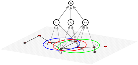
Figure 2: In a compositional network each neuron $\mathfrak{n}$ is only equivariant to the permutations of a subset of objects $\mathop{\mathrm{dom}}(\mathfrak{n})\subseteq\mathcal{O}$. Here, for example, $\mathfrak{n}_{1}$ captures information from vertices $\{v_{1},v_{2},v_{3}\}$; $\mathfrak{n}_{2}$ from $\{v_{2},v_{3},v_{4}\}$; and $\mathfrak{n}_{3}$ from $\{v_{2},v_{3},v_{4},v_{5}\}$. When the outputs of these three neurons are aggregated in a higher level neuron, whose domain covers all five vertices, the outputs of $\mathfrak{n}_{1},\mathfrak{n}_{2}$ and $\mathfrak{n}_{3}$ must be promoted to transform equivariantly wrt. $\mathbb{S}_{5}$.

The above definition captures the natural way in which any network that involves a hierarchical decomposition of a complex objects into parts is expected to behave. Informally, the definition says that each neuron is only responsible for a subset of objects ($\smash{\mathop{\mathrm{dom}}(\mathfrak{n})}$) and if the objects are permuted by $\sigma$, then the output of the neuron is going to transform according the restriction of $\sigma$ to this subset, which is $\pi$. For example, message passing neural networks follow this schema with $\mathop{\mathrm{dom}}(\mathfrak{n})$ being the $1$-neighborhoods, $2$-neighborhoods, etc., of each vertex. However, in most MPNNs the activations are invariant under permutations, which corresponds to $\{T^{\mathfrak{n}}_{\pi}\}$ being the trivial action of $\smash{\mathbb{S}_{\left|\mathop{\mathrm{dom}}{\mathfrak{n}}\right|}}$. If we want to capture a richer set of interactions, specifically interactions where the output of $\mathfrak{n}$ retains information about the individual identities of the objects in its domain, relations between the objects, or their relative rankings, for example, then it is essential that the outputs of the neurons be allowed to vary with higher order permutation actions (Figure 2).

Each neuron in a compositional architecture aggregates information related to $\smash{\mathop{\mathrm{dom}}(\mathfrak{n}_{c_{1}}),\ldots,\mathop{\mathrm{dom}}(\mathfrak{n}_{c_{k}})\subseteq\mathop{\mathrm{dom}}(\mathfrak{n})}$ to $\smash{\mathop{\mathrm{dom}}(\mathfrak{n})}$ itself. Being able to do this without losing equivariance requires knowing the correspondence between each element of $\smash{\mathop{\mathrm{dom}}(\mathfrak{n}_{c_{p}})}$ and $\smash{\mathop{\mathrm{dom}}(\mathfrak{n})}$. To be explicit, we will denote which element of $\smash{\mathop{\mathrm{dom}}(\mathfrak{n})}$ any given $\smash{i\in\mathop{\mathrm{dom}}(\mathfrak{n}_{c_{p}})}$ corresponds to by $\chi^{\mathfrak{n}}_{p}(i)$, and we will call promotion the act of reindexing each incoming activation $\smash{f^{\mathfrak{n}_{c_{p}}}}$ to transform covariantly with permutations of the larger set $\smash{\mathop{\mathrm{dom}}(\mathfrak{n})}$. The promoted version of $\smash{f^{\mathfrak{n}_{c_{p}}}}$ we denote $\smash{\widetilde{f}{}^{\mathfrak{n}_{c_{p}}}}$. In the case of first, second, etc., order activations stored in vector/matrix/tensor form, promotion corresponds to simple reindexing:

$$[\widetilde{f}{}^{\mathfrak{n}_{c_{p}}}]_{\chi^{\mathfrak{n}}_{p}(i)}=[f^{\mathfrak{n}_{c_{p}}}]_{i},\quad[\widetilde{f}{}^{\mathfrak{n}_{c_{p}}}]_{\chi^{\mathfrak{n}}_{p}(i),\hskip 0.70004pt\chi^{\mathfrak{n}}_{p}(j)}=[f^{\mathfrak{n}_{c_{p}}}]_{i,j}.$$ (6)

In the case of Fourier space activations, with the help of FFT methods, computing each $\smash{\widetilde{F}{}^{\mathfrak{n}_{c_{p}}}_{i}}$ takes $\smash{O((|\mathop{\mathrm{dom}}(\mathfrak{n})|-|\mathop{\mathrm{dom}}(\mathfrak{n}_{c_{p}})|)\hskip 1.00006ptd_{\lambda_{i}}\hskip 1.00006pt\tau_{i})}$ operations. Describing this process in detail is unforutnately beyond the scope of the present paper.

Once promoted, $\smash{\widetilde{f}{}^{\mathfrak{n}_{c_{1}}},\ldots,\widetilde{f}{}^{\mathfrak{n}_{c_{k}}}}$ must be combined in a way that is itself covariant with permutations of $\mathop{\mathrm{dom}}(\mathfrak{n})$. The simple way to do this is to just to sum them. For example, in a second order network, using Theorem 2 we might have

$$f^{out}_{i,j}=\xi\bigl{(}w_{0}\bar{f}_{i,j}+w_{1}\bar{f}_{j,i}+w_{2}\bar{f}_{i,\ast}+w_{3}\bar{f}_{\ast,i}+\\ w_{4}\bar{f}_{\ast,j}+w_{5}\bar{f}_{j,\ast}+w_{6}\bar{f}_{\ast,\ast}\bigr{)},$$

where $\bar{f}=\sum_{i}\widetilde{f}{}^{\mathfrak{n}_{c_{k}}}$. This type of aggregation rule is similar to the summation operation used in MPNNs. In particular, while it correctly accounts for the overlap between the domains of upstream neurons, it does not take into account which $\smash{\widetilde{f}{}^{\mathfrak{n}_{c_{i}}}}$ relates to which subset of $\mathop{\mathrm{dom}}(\mathfrak{n})$. A richer class of models is obtained by forming potentially higher order covariant products of the promoted incoming activations rather than just sums. Such networks are still covariant but go beyond the mold of convolutional nets because by virtue of the nonlinear interaction, one input to the given neuron can modulate the other inputs.

6 Second order permutation equivariant variational graph auto-encoder

To demonstrate the power of higher-order permutation-equivariant layers, we apply them to the problem of graph learning, where the meaning of both equivariance and compositionality is very intuitive. We focus on generative models rather than just learning from graphs, as the exact structure of the graph is uncertain. Consequently, edges over all possible pairs of nodes must, at least in theory, be considered. This makes a natural connection with the permutation group.

Variational Auto-encoders (VAE’s) consist of an encoder/decoder pair where the encoder learns a low dimensional representation of, while the decoder learns to reconstruct using a simple probabilistic model on a latent representation.(Kingma & Welling, 2013) The objective function combines two terms: the first term measures how well the decoder can reconstruct each input in the training set from its latent representation, whereas the second term aims to ensure that the distribution corresponding to the training data is as close as possible to some fixed target distribution such as a multivariate normal. After training, sampling from the target distribution, possibly with constraints, will generate samples that are similar to those in the training set.

Equivariance is important when constructing VAE’s for graphs because in order to compare each input graph to the output graph generated by the decoder, the network needs to know which input vertex corresponds to which output vertex. This allows the quality of the reconstruction to be measured without solving an expensive graph-matching problem. The first architectures were based on spectral ideas, in which case equivariance comes “for free” (Kipf & Welling, 2016). However, spectral VGAE’s are limited in the extent to which they can capture the combinatorial structure of graphs because they draw every edge independently (albeit with different parameters).

An alternative approach is to generate the output graph in a sequential manner, somewhat similarly to how RNNs and LSTMs generate word sequences (You et al., 2018)(Liao et al., 2019). These methods can incorporate rich local information in the generative process, such as a library of known functional groups in chemistry applications. On the other hand, this can break the direct correspondence between the vertices of the input graph and the output graph, so the loss function can only compare them via global graph properties such as the frequency of certain small subgraphs, etc..

6.1 The latent layer

To ensure end-to-end equivariance, we set the latent layer to be a matrix $P\in\mathbb{R}^{n\times C}$, whose first index is first order equivariant with permutations. At training time, $P$ is computed from $\smash{f^{\mathfrak{n}^{\textrm{top}}}_{i,j,a}}$ simply by summing over the $j$ index. For generating new graphs, however, we must specify a distribution for $P$ that is invariant to permutations. In the language of probability theory, such distributions are called exchangeable (Kallenberg, 2006).

For infinite exchangeable sequences de Finetti’s theorem states that any such distribution is a mixture of iid. distributions (De Finetti, 1930). For finite dimensional sequences the situation is somewhat more complicated (Diaconis & Freedman, 1980). Recently a number of researchers have revisited exchangeability from the perspective of machine learning, and specifically graph generation (Orbanz & Roy, 2015)(Cai et al., 2016)(Bloem-Reddy & Teh, 2019).

Link prediction on citation graphs.

To demonstrate the efficacy of higher order ${\mathbb{S}_{n}}$-equivariant layers, we compose them with the original VGAE architecture in (Kipf & Welling, 2016). While this architecture is a key historical benchmark on link-prediction tasks, it has the drawback that the encoder takes the form $\xi\left(zz^{\top}\right)$, where $z$ is the value of the graph encoded in the latent layer. Effectively, the decoder of the graph has no hidden layers, which limits its expressive power. However, we show that if this can be mitigated by composing the same architecture with ${\mathbb{S}_{n}}$-convolutional layers. Specifically, we place additional convolutional layers between the outer product $zz^{\top}$ and the final sigmoid, interspersed with ReLU nonlinearities. We then apply the resulting network to link prediction on the citation network datasets Cora and Citeseer (Sen et al., 2008). In training time, 15% of the citation links (edges) have been removed while all node features are kept. The models are trained on an incomplete graph Laplacian constructed from the remaining 85% of the edges. From previously removed edges, we sample the same number of pairs of unconnected nodes (non-edges). We form the validation and test sets that contain 5% and 10% of edges with an equal amount of non-edges, respectively. Hyperparameters optimization (e.g. number of layers, dimension of the latent representation, etc.) is done on the validation set.

We then compare the architecture against the original (variational) graph autoencoder (Kipf & Welling, 2016), as well as spectral clustering (SC) (Tang & Liu, 2011), deep walk (DW) (Perozzi et al., 2014), and GraphStar (Haonan et al., 2019) and compare the ability to correctly classify edges and non-edges using two metrics: area under the ROC curve (AUC) and average precision (AP). Numerical results of SC, DW, GAE and VGAE and experimental settings are taken from (Kipf & Welling, 2016). We initialize weights by Glorot initialization (Glorot & Bengio, 2010). We train for 2,048 epochs using Adam optimization (Kingma & Ba, 2015) with a starting learning rate of $0.01$. The number of layers range from 1 to 4. The size of latent representation is 64.

Method	AUC	AP
SC	84.6 $\pm$ 0.01	88.5 $\pm$ 0.00
DW	83.1 $\pm$ 0.01	85.0 $\pm$ 0.00
GAE	91.0 $\pm$ 0.02	92.0 $\pm$ 0.03
VGAE	91.4 $\pm$ 0.01	92.6 $\pm$ 0.01
GraphStar	95.65 $\pm$ ?	96.15 $\pm$ ?
2nd order VGAE (our method)	96.1 $\pm$ 0.07	96.4 $\pm$ 0.06

Table 1: Cora link prediction results (AUC & AP)

Method	AUC	AP
SC	80.5 $\pm$ 0.01	85.0 $\pm$ 0.01
DW	80.5 $\pm$ 0.02	83.6 $\pm$ 0.01
GAE	89.5 $\pm$ 0.04	89.9 $\pm$ 0.05
VGAE	90.8 $\pm$ 0.02	92.0 $\pm$ 0.02
GraphStar	97.47 $\pm$ ?	97.93 $\pm$ ?
2nd order VGAE (our method)	95.3 $\pm$ 0.02	94.3 $\pm$ 0.02

Table 2: Citeseer link prediction results (AUC & AP)

We found that these additional layers make VGAE so expressive it quickly overfits. We consequently regularize the models through early stopping. Tables 1 and 2 show our numerical results in Cora and Citeseer datasets. We give the performance of our best model for each task, as well as the performance from only adding a single layer to VGAE. Our results improve over the original VGAE architecture in all categories. For Cora, VGAE becomes competitive with more recent architectures such as GraphStar. Moreover, we see that already a single layer of the second-order equivariant gives a tangible improvement over the previous VGAE results.

Molecular generation.

We next explore the ability of ${\mathbb{S}_{n}}$-equivariant layers to build graphs with highly structured graphs by applying them to the task of molecular generation. We do not incorporate any domain knowledge in our architecture; the only input to the network is a one-hot vector of the atom identities and the adjacency matrix. As we intend to only test the expressive power of the convolutional layers, here we construct both the encoder and the decoder using activations of the form in 4 with ReLU nonlinearities. Node features can be incorporated naturally as a second-order features with zero off-diagonal elements. Similar to (V)GAE, we use a latent layer of shape $n\times c$, where $c$ is a the size of the latent embedding for each node. To do form the values in the latent layer, we take a linear combination of first-order terms in Corollary 4,

$$f^{\textrm{latent}}_{i}=\xi\bigl{(}w_{1}f^{\textrm{in}}_{i,\ast}+w_{2}f^{\textrm{in}}_{\ast,i}+w_{3}f^{\textrm{in}}_{\ast,\ast}+w_{4}\overline{f^{\textrm{in}}_{\ast}}+w_{5}f^{\textrm{in}}_{i,i}\bigr{)}.$$ (7)

We take our target distribution in the variational autoencoder to be $\smash{\mathcal{N}\left(0,1\right)}$ on this space, independently on all of the entries. To reconstruct a second-order feature from the latent layer in the decoder, we take the tensor product of each channel of $f^{\textrm{latent}}_{i}$ to build a collection of rank one second-order features. The rest of the decoder then consists of layers formed as described in Corollary 4. In the final layer we apply a sigmoid to a predicted tensor of size $n\times n\times 3$. This tensor represents our estimate of the labelled adjacency matrix, which should $1$ in the $i,j,k$’th element if atoms $i$ and $j$ are connected by a bond of type $k$ in the (kekulized) molecule. Similarly, we also predict atom labels by constructing a first-order feature as in (7) with the number of channels equal to the number of possible atoms and apply a softmax across channels. The accuracy of our estimate is then evaluated using a binary cross-entropy loss to the predicted bonds and a negative log-likelihood loss to the predicted atom labels. To actually generate the molecule, we choose the atom label with largest value in the softmax, and connect it with all other atoms where our bond prediction tensor is larger than $0.5$.

To test this architecture, we apply it to the ZINC dataset (Sterling & Irwin, 2015) and attempt to both encode the molecules in the dataset and generate new molecules. Both the encoder and the decoder have 4 layers of with 100 channel indices with a ReLU nonlinearity, and we set the latent space to be of dimension $n_{max}\times 20$, where $n_{max}$ is the largest molecule in the dataset (smaller molecules are treated using disconnected ghost atoms). We train for 256 epochs, again using the Adam algorithm.(Kingma & Ba, 2015) Interestingly, we achieved better reconstruction accuracy and generated molecules when disabling the KL divergence term in the VAE loss function. We discuss potential reasons for this in the supplement.

To evaluate the accuracy of the encodings, we evaluate the reconstruction accuracy using the testing split described in (Kusner et al., 2017). In table 3, we report numerical results for two metrics: reconstruction accuracy of molecules in the test set, and validity of new molecules generated from the prior and compare with other algorithms.

Method	Accuracy	Validity
CVAE	44.6%	0.7%
GVAE	53.7%	7.2%
SD-VAE	76.2%	43.5%
GraphVAE	-	13.5%
Atom-by-Atom LSTM	-	89.2%
JT-VAE	76.7 %	100.0%
2nd order ${\mathbb{S}_{n}}$-Conv VAE (our method)	98.4%	33.4%

Table 3: ZINC results (reconstruction accuracy & validity)

Our algorithm gives the best reconstruction among the accuracies considered. Moreover, we note that our algorithm requires considerably less domain knowledge than many of the other algorithms in Table 3. The SD-VAE, Grammar VAE (GVAE) (Kusner et al., 2017), and Character VAE (CVAE) (Gomez-Bombarelli et al., 2016) treat the task of molecular graph generation as text generation in Natural Language Processing by explicitly using the SMILES strings: structured representations of molecules that, in their construction, encode rules about chemical connectivity. JT-VAE explicitly draws from a vocabulary of chemical structures and explicitly ensures that the output obeys known chemical rules. In contrast, our model is given no knowledge of basic chemical principles such as valency or of functional groups, and must learn it from first principles.

To test the validity of newly generated molecules, we take 5000 samples from our target distribution, feed them into the decoder, and determine how many correspond to valid SMILES strings using RDKit. Our model does not learn to construct construct a single, connected graph; consequently we take the largest connected component of the graph as our predicted molecule. Perhaps a result of our procedure for reading the continuous bond features into a single molecule with discrete bonds, we find that our results are biased towards small molecules: roughly 20 percent of the valid molecules we generate have 5 heavy atoms or less. In figure 3 we give a random sample of 12 of the generated molecules that are syntactically valid and have more than 10 atoms. Comparing with the molecules in the ZINC dataset, our network constructs many molecules that are sterically strained. Many generated molecules have 4-atom rings, features which are rare seen in stable organic molecules. Indeed, the ability to make inferences over types of molecular rings is an example of higher-order information, requiring direct comparison over multiple atoms at once. However, we note that our model is able to construct molecules with relatively reasonable bonding patterns and carbon backbones. In conjunction with our reconstruction results, we believe that even simple higher-order information can be used to infer more complex graph structure.

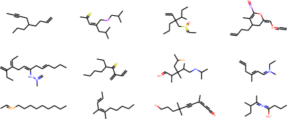
Figure 3: A sample of 12 molecules of generated by the second-order graph variational autoencoder. Molecules are constrained to be syntactically valid (can be converted into valid SMILES strings) and have more than 10 atoms.

7 Conclusions

In this paper we argued that to fully take into account the action of permutations on neural networks, one must consider not just the defining representation of ${\mathbb{S}_{n}}$, but also some of the higher order irreps. This situation is similar to, for example, recent work on spherical CNNs, where images on the surface of the sphere are expressed in terms of spherical harmonics up to a specific order (Cohen et al., 2018). Specifically, to correctly learn $k$’th order relations between members of a set requires a $k$’th order permutation equivariant architecture.

Graphs are but the simplest case of this, since whether or not two vertices are connected by an edge is a second order relationship. Already in this case, our experiments on link prediction and molecule generation show that equivariance gives us an edge over other algorithms, which is noteworthy given that the other algorithms use hand crafted chemical features (or rules). Going further, a 4th order equivariant model for example could learn highly specific chemical rules by itself relating to quadruples of atoms, such as “when do these four atoms form a peptide group?”. Higher order relation learning would work similarly.

Interestingly, permutation equivariant generative models are also related to the theory of finite exchangeable sequences, which we plan to explore in future work.

8 Appendix A:  Supporting propositions

Proposition 5.

Let $f\in\mathbb{R}^{n}$ be any vector on which ${\mathbb{S}_{n}}$ acts by the first order permutation action

$$f\overset{\sigma}{\longmapsto}f^{\sigma}\qquad\text{with}\qquad f^{\sigma}=(f_{\sigma^{-1}(1)},\ldots,f_{\sigma^{-1}(n)})\qquad\quad\sigma\in{\mathbb{S}_{n}}.$$

Let us associate to $f$ the function $\mathfrak{f}\colon{\mathbb{S}_{n}}/\mathbb{S}_{n-1}\to\mathbb{R}$ defined

$$\mathfrak{f}(\mu)=f_{\mu(n)}\qquad\quad\qquad\quad\mu\in\mathcal{R},$$ (8)

where $\mathcal{R}$ is a complete set of ${\mathbb{S}_{n}}/\mathbb{S}_{n-1}$ coset representatives. Then, the mapping $f\mapsto\mathfrak{f}$ is bijective. Moreover, under permutations $\smash{\mathfrak{f}\mapsto\mathfrak{f}^{\sigma}}$ with $\smash{\mathfrak{f}^{\sigma}(\mu)=\mathfrak{f}(\sigma^{-1}\mu)}$.

Proof. Recall that ${\mathbb{S}_{n}}/\mathbb{S}_{n-1}$ is defined as the collection of left cosets $\smash{\{\mu\,\mathbb{S}_{n-1}\}_{\mu}}$ with $\smash{\mu\hskip 1.00006pt\mathbb{S}_{n-1}\!:=\!\{\hskip 1.00006pt{\mu\nu}\>|\>{\nu\in\mathbb{S}_{n-1}\hskip 1.00006pt}\}\subset{\mathbb{S}_{n}}}$. Any member of a given coset can be used to serve as the representative of that coset. Therefore, we first need to verify that (8) is well defined, i.e., that $\mu(n)=(\mu\nu)(n)$ for any $\nu\in\mathbb{S}_{n-1}$. Since $(\mu\nu)(n)=\mu(\nu(n))$ and $\nu$ fixes $n$, this is clearly true.

Now, for any $i\in\{1,2,\ldots,n\}$ there is exactly one coset $\mu\hskip 1.00006pt\mathbb{S}_{n-1}$ such that $\mu(n)=i$ Therefore, the mapping $f\mapsto\mathfrak{f}$ is bijective. Finally, to show that $\mathfrak{f}$ transforms correctly consider that $\mathfrak{f}^{\sigma}(\mu):=(f^{\sigma})_{\mu(n)}=f_{\sigma^{-1}(\mu(n))}=f_{(\sigma^{-1}\mu)(n)}=\mathfrak{f}(\sigma^{-1}\mu)$. $\blacksquare$

The second order case is analogous with the only added complication that to ensure bijectivity we need to require that the activation as a matrix be symmetric and have zero diagonal. For the adjacency matrices of simple graphs these conditions are satisfied automatically.

Proposition 6.

Let $F\in\mathbb{R}^{n\times n}$ be a matrix with zero diagonal on which ${\mathbb{S}_{n}}$ acts by the second order permutation action

$$F\overset{\sigma}{\longmapsto}F^{\sigma}\qquad\text{with}\qquad F^{\sigma}_{i,j}=F_{\sigma^{-1}(i),\hskip 0.70004pt\sigma^{-1}(j)}\qquad\quad\sigma\in{\mathbb{S}_{n}}.$$

Let us associate to $F$ the function $\mathfrak{f}\colon{\mathbb{S}_{n}}/\mathbb{S}_{n-2}\to\mathbb{R}$ defined

$$\mathfrak{f}(\mu)=F_{\mu(n),\,\mu(n-1)}\qquad\quad\mu\in\mathcal{R},$$ (9)

where $\mathcal{R}$ is a complete set of ${\mathbb{S}_{n}}/\mathbb{S}_{n-1}$ coset representatives. Then, the mapping $F\mapsto\mathfrak{f}$ is bijective. Moreover, under permutations $\smash{\mathfrak{f}\mapsto\mathfrak{f}^{\sigma}}$ with $\mathfrak{f}^{\sigma}(\mu)=\mathfrak{f}(\sigma^{-1}\mu)$.

Proof. The proof is analogous to the first order case. First, ${\mathbb{S}_{n}}/\mathbb{S}_{n-2}$ is the set of left cosets of the form $\smash{\mu\hskip 1.00006pt\mathbb{S}_{n-2}\!:=\!\{\hskip 1.00006pt{\mu\nu}\>|\>{\nu\in\mathbb{S}_{n-2}\hskip 1.00006pt}\}}$. Since any $\nu\in\mathbb{S}_{n-2}$ fixes $\{n,n-1\}$, for any $\mu\nu\in\mu\hskip 1.00006pt\mathbb{S}_{n-2}$, $\mu\nu(n)=\mu(n)$ and $\mu\nu(n-1)=\mu(n-1)$. Therefore $\mathfrak{f}$ is well defined.

It is also easy to see that for any $(i,j)$ pair with $i,j\in\{1,2,\ldots,n\}$ and $i\neq j$, then there is exactly one $\mu\,\mathbb{S}_{n-2}$ coset satisfying $\mu(n)=i$ and $\mu(n-1)=j$. Finally, to show that $\mathfrak{f}$ transforms correctly, $\smash{\mathfrak{f}^{\sigma}(\mu)=(F^{\sigma})_{\mu(n),\hskip 0.70004pt\mu(n-1)}=F_{\sigma^{-1}(\mu(n)),\hskip 0.70004pt\sigma^{-1}(\mu(n-1))}=F_{(\sigma^{-1}\mu)(n),\,(\sigma^{-1}\mu)(n-1)}=\mathfrak{f}(\sigma^{-1}\mu)}$. $\blacksquare$

Proposition 7.

Let $F\in\mathbb{R}^{n\times\ldots\times n}$ be a $k$’th order tensor satisfying $F_{i_{1},\ldots,i_{k}}=0$ unless $i_{1},\ldots,i_{k}$ are all distinct. Assume that ${\mathbb{S}_{n}}$ acts on $F$ by the $k$’th order permutation action

$$F\overset{\sigma}{\longmapsto}F^{\sigma}\qquad\text{with}\qquad F^{\sigma}_{i_{1},\ldots,i_{k}}=F_{\sigma^{-1}(i_{1}),\ldots,\sigma^{-1}(i_{k})}\qquad\quad\sigma\in{\mathbb{S}_{n}}.$$

Let us associate to $F$ the function $\mathfrak{f}\colon{\mathbb{S}_{n}}/\mathbb{S}_{n-k}\to\mathbb{R}$ defined

$$\mathfrak{f}(\mu)=F_{\mu(n),\ldots,\mu(n-k+1)}\qquad\quad\mu\in\mathcal{R},$$ (10)

where $\mathcal{R}$ is a complete set of ${\mathbb{S}_{n}}/\mathbb{S}_{n-k}$ coset representatives. Then, the mapping $F\mapsto\mathfrak{f}$ is bijective. Moreover, under permutations $\smash{\mathfrak{f}\mapsto\mathfrak{f}^{\sigma}}$ with $\mathfrak{f}^{\sigma}(\mu)=\mathfrak{f}(\sigma^{-1}\mu)$.

Proof.  Analogous to the first and and second order cases.

9 Appendix B:  Proofs

Proof of Theorem 1. Let $\mathfrak{f}^{\textrm{in}}$ and $\mathfrak{f}^{\textrm{out}}$ be the quotient space functions corresponding to $f^{\textrm{in}}$ and $f^{out}$. Then, by Theorem 1 of (Kondor & Trivedi, 2018),

$$\mathfrak{f}^{\textrm{out}}(\mu)=\xi\biggl{(}\>\sum_{\nu\in{\mathbb{S}_{n}}}\mathfrak{f}^{\textrm{in}}(\mu\nu^{-1})\,\chi(\nu)\biggr{)}$$

for some appropriate pointwise nonlinearity $\xi$ and some (learnable) filter $\chi\colon\mathbb{S}_{n-1}\backslash{\mathbb{S}_{n}}/\mathbb{S}_{n-1}\to\mathbb{R}$. Alternatively, mapping $\mathfrak{f}^{\textrm{out}}$ back to vector form, we can write

$$f^{out}_{i}=\xi(\tilde{f}_{i})\qquad\quad\qquad\quad\tilde{f}_{i}=\sum_{\nu\in{\mathbb{S}_{n}}}\mathfrak{f}^{\textrm{in}}(\mu_{i}\nu^{-1})\,\chi(\nu),$$

where $\mu_{i}$ denote the representative of the coset that maps $n\mapsto i$,

Let $e$ denote the identity element of ${\mathbb{S}_{n}}$ and $\tau_{n,n-1}\in{\mathbb{S}_{n}}$ denote the element that swaps $n$ and $n-1$. There are only two $\mathbb{S}_{n-1}\backslash{\mathbb{S}_{n}}/\mathbb{S}_{n-1}$ cosets:

$$S_{0}=\mathbb{S}_{n-1}e\,\mathbb{S}_{n-1}=\left\{\,{\mu\in{\mathbb{S}_{n}}}\>\middle|\>{\mu(n)=n\,}\right\}$$

$$S_{1}=\mathbb{S}_{n-1}\tau_{n,n-1}\,\mathbb{S}_{n-1}=\left\{\,{\mu\in{\mathbb{S}_{n}}}\>\middle|\>{\mu(n)\neq n\,}\right\}.$$

Assume that $\chi$ takes on the value $\chi_{0}$ on $S_{0}$ and the value $\chi_{1}$ on $S_{1}$. Then

$$\tilde{f}_{i}=\sum_{\nu\in S_{0}}\mathfrak{f}^{\textrm{in}}(\mu_{i}\nu^{-1})\,\chi(\nu)+\sum_{\nu\in S_{1}}\mathfrak{f}^{\textrm{in}}(\mu_{i}\nu^{-1})\,\chi(\nu).$$

For the $\nu\in S_{0}$ case note that $\left|S_{0}\right|=(n-1)!$ and that $\mu$ and $\mu\nu^{-1}$ will always fall in the same left $\mathbb{S}_{n-1}$-coset. Therefore,

$$\sum_{\nu\in S_{0}}\mathfrak{f}^{\textrm{in}}(\mu_{i}\nu^{-1})\,\chi(\nu)=\chi_{0}\sum_{\nu\in S_{0}}\mathfrak{f}^{\textrm{in}}(\mu_{i}\nu^{-1})=(n-1)!\>\chi_{0}\>\mathfrak{f}^{\textrm{in}}(\mu_{i})=(n-1)!\>\chi_{0}\>f^{\textrm{in}}_{i}.$$

For the $\nu\in S_{1}$ case note that $\nu$ as traverses $S_{1}$, $\mu\nu^{-1}$ will never fall in the same coset as $\mu$, but will fall in each of the other cosets exactly $(n-1)!$ times. Therefore,

$$\sum_{\nu\in S_{1}}\mathfrak{f}^{\textrm{in}}(\mu_{i}\nu^{-1})\,\chi(\nu)=\chi_{1}\sum_{\nu\in S_{1}}\mathfrak{f}^{\textrm{in}}(\mu_{i}\nu^{-1})=(n-1)!\>\chi_{0}\!\!\!\!\!\sum_{\begin{subarray}{c}\pi\in{\mathbb{S}_{n}}/\mathbb{S}_{n-1}\\ \pi\not\in\mu_{i}\mathbb{S}_{n-1}\end{subarray}}\!\!\!\!\mathfrak{f}^{\textrm{in}}(\pi)=(n-1)!\>\chi_{0}\sum_{j\neq i}f^{\textrm{in}}_{j}.$$

Combining the above,

$$f^{out}_{i}=\xi\Bigl{[}(n-1)!\>\Bigl{(}\chi_{0}\,f^{\textrm{in}}_{i}+\chi_{1}\sum_{j\neq i}f^{\textrm{in}}_{j}\Bigr{)}\Bigr{]}=\xi\Bigl{[}(n-1)!\>\Bigl{(}\chi_{0}\,f^{\textrm{in}}_{i}+\chi_{1}\sum_{j}f^{\textrm{in}}_{j}-\chi_{1}f^{\textrm{in}}_{i}\Bigr{)}\Bigr{]}.$$

Setting $w_{0}=(n-1)!(\chi_{0}-\chi_{1})$ and $w_{1}=(n-1)!\>\chi_{1}$ proves the result. $\blacksquare$

Proof of Theorem 2. Let $\mathfrak{f}^{\textrm{in}}$, $\mathfrak{f}^{\textrm{out}}$, $\tau_{i,j}$ and $\chi$ be as in the proof of Theorem 1. Now, however, $f$ is indexed by two indices, $i,j\in\{1,2,\ldots,n\}$ and $i\neq j$. Correspondingly, we let $\mu_{i}$ denote the representative of the $\mathbb{S}_{n-2}$–coset consisting of permutations that take $n\mapsto i$ and $n-1\mapsto j$. Similarly to the proof of Theorem 1, we set

$$f^{out}_{i,j}=\xi(\tilde{f}_{i,j})\qquad\quad\qquad\quad\tilde{f}_{i,j}=\sum_{\nu\in{\mathbb{S}_{n}}}\mathfrak{f}^{\textrm{in}}(\mu_{i,j}\nu^{-1})\,\chi(\nu),\vspace{-6pt}$$

where now $\chi\colon\mathbb{S}_{n-2}\backslash{\mathbb{S}_{n}}/\mathbb{S}_{n-2}\to\mathbb{R}$.

There are a rotal of seven $\mathbb{S}_{n-2}\backslash{\mathbb{S}_{n}}/\mathbb{S}_{n-2}\to\mathbb{R}$ cosets:

$$S_{0}=\mathbb{S}_{n-2}\,e\,\mathbb{S}_{n-2}=\left\{\,{\mu\in{\mathbb{S}_{n}}}\>\middle|\>{\mu(n)=n,~{}\mu(n-1)=n-1\,}\right\}$$

$$S_{1}=\mathbb{S}_{n-2}\,\tau_{n,n-1}\,\mathbb{S}_{n-2}=\left\{\,{\mu\in{\mathbb{S}_{n}}}\>\middle|\>{\mu(n)=n-1,~{}\mu(n-1)=n\,}\right\}$$

$$S_{2}=\mathbb{S}_{n-1}\,\tau_{n-1,n-2}\,\mathbb{S}_{n-1}=\left\{\,{\mu\in{\mathbb{S}_{n}}}\>\middle|\>{\mu(n)=n,~{}\mu(n-1)\in\{1,\ldots,n-2\}\,}\right\},$$

$$S_{3}=\mathbb{S}_{n-1}\,\tau_{n,n-1}\,\tau_{n-1,n-2}\,\mathbb{S}_{n-1}=\left\{\,{\mu\in{\mathbb{S}_{n}}}\>\middle|\>{\mu(n)=n-1,~{}\mu(n-1)\in\{1,\ldots,n-2\}\,}\right\},$$

$$S_{4}=\mathbb{S}_{n-1}\,\tau_{n,n-2}\,\mathbb{S}_{n-1}=\left\{\,{\mu\in{\mathbb{S}_{n}}}\>\middle|\>{\mu(n)\in\{1,\ldots,n-2\},~{}\mu(n-1)=n-1\,}\right\},$$

$$S_{5}=\mathbb{S}_{n-1}\,\tau_{n,n-1}\,\tau_{n,n-2}\,\mathbb{S}_{n-1}=\left\{\,{\mu\in{\mathbb{S}_{n}}}\>\middle|\>{\mu(n)\in\{1,\ldots,n-2\},~{}\mu(n-1)=n\,}\right\},$$

$$S_{6}=\mathbb{S}_{n-1}\,\tau_{n,n-2}\,\tau_{n-1,n-3}\,\mathbb{S}_{n-1}=\left\{\,{\mu\in{\mathbb{S}_{n}}}\>\middle|\>{\mu(n)\in\{1,\ldots,n-2\},~{}\mu(n-1)\in\{1,\ldots,n-2\}\,}\right\}.$$

Assuming that $\chi$ takes on the values $\chi_{0},\ldots,\chi_{6}$ on these seven cosets,

$$\tilde{f}_{i,j}=\sum_{p=0}^{6}\>\chi_{p}\!\underbrace{\sum_{\nu\in S_{p}}\mathfrak{f}^{\textrm{in}}(\mu_{i,j}\nu^{-1})}_{h_{i,j}^{p}}.\vspace{-6pt}$$

Now we analyze the $p=0,1,\ldots,6$ cases separately.

1. In the $p=0$ case $\left|S_{0}\right|=(n-2)!$  and  $\mu_{i,j}\nu^{-1}\!\in\mu_{i,j}\hskip 1.00006pt\mathbb{S}_{n-1}$, therefore

   $$h_{i,j}^{0}=\sum_{\nu\in S_{0}}\mathfrak{f}^{\textrm{in}}(\mu_{i,j}\nu^{-1})=(n-2)!\>f^{\textrm{in}}_{i,j}.$$

2. In the $p=1$ case $\left|S_{1}\right|=(n-2)!$  and  $\mu_{i,j}\nu^{-1}\!\in\mu_{j,i}\hskip 1.00006pt\mathbb{S}_{n-1}$, therefore

   $$h_{i,j}^{1}=\sum_{\nu\in S_{1}}\mathfrak{f}^{\textrm{in}}(\mu_{i,j}\nu^{-1})=(n-2)!\>f^{\textrm{in}}_{j,i}.$$

3. In the $p=2$ case, as $\nu$ traverses $S_{2}$,  $\mu_{i,j}\nu^{-1}$ will hit each $\mu_{i,k}\hskip 1.00006pt\mathbb{S}_{n-2}$ coset with $k\!\not\in\!\{i,j\}$ exactly $(n-2)!$ times, therefore

   $$h_{i,j}^{2}=\sum_{\nu\in S_{2}}\mathfrak{f}^{\textrm{in}}(\mu_{i,j}\nu^{-1})=(n-2)!\>\sum_{k\not\in\left\{i,j\right\}}f^{\textrm{in}}_{i,k}.$$

4. In the $p=3$ case, as $\nu$ traverses $S_{3}$,  $\mu_{i,j}\nu^{-1}$ will hit each $\mu_{k,i}\hskip 1.00006pt\mathbb{S}_{n-2}$ coset with $k\!\not\in\!\{i,j\}$ exactly $(n-2)!$ times, therefore

   $$h_{i,j}^{3}=\sum_{\nu\in S_{3}}\mathfrak{f}^{\textrm{in}}(\mu_{i,j}\nu^{-1})=(n-2)!\>\sum_{k\not\in\left\{i,j\right\}}f^{\textrm{in}}_{k,i}.$$

5. In the $p=4$ case, as $\nu$ traverses $S_{4}$,  $\mu_{i,j}\nu^{-1}$ will hit each $\mu_{k,j}\hskip 1.00006pt\mathbb{S}_{n-2}$ coset with $k\!\not\in\!\{i,j\}$ exactly $(n-2)!$ times, therefore

   $$h_{i,j}^{4}=\sum_{\nu\in S_{4}}\mathfrak{f}^{\textrm{in}}(\mu_{i,j}\nu^{-1})=(n-2)!\>\sum_{k\not\in\left\{i,j\right\}}f^{\textrm{in}}_{k,j}.$$

6. In the $p=5$ case, as $\nu$ traverses $S_{5}$,  $\mu_{i,j}\nu^{-1}$ will hit each $\mu_{j,k}\hskip 1.00006pt\mathbb{S}_{n-2}$ coset with $k\!\not\in\!\{i,j\}$ exactly $(n-2)!$ times, therefore

   $$h_{i,j}^{5}=\sum_{\nu\in S_{5}}\mathfrak{f}^{\textrm{in}}(\mu_{i,j}\nu^{-1})=(n-2)!\>\sum_{k\not\in\left\{i,j\right\}}f^{\textrm{in}}_{j,k}.$$

7. In the $p=6$ case, as $\nu$ traverses $S_{6}$,  $\mu_{i,j}\nu^{-1}$ will hit each $\mu_{k,l}\hskip 1.00006pt\mathbb{S}_{n-2}$ coset with $k\!\not\in\!\{i,j\}$ and $l\!\not\in\!\{i,j\}$ exactly $(n-2)!$ times, therefore

   $$h_{i,j}^{6}=\sum_{\nu\in S_{6}}\mathfrak{f}^{\textrm{in}}(\mu_{i,j}\nu^{-1})=(n-2)!\>\sum_{k,l\not\in\left\{i,j\right\}}f^{\textrm{in}}_{k,l}.$$

Summing each of the above terms gives

$$f^{out}_{i,j}=\xi\Bigl{(}(n-2)!\>\bigl{(}\chi_{0}\hskip 1.00006ptf^{\textrm{in}}_{i,j}+\chi_{1}\hskip 1.00006ptf^{\textrm{in}}_{j,i}+\chi_{2}(f^{\textrm{in}}_{i,\ast}-f^{\textrm{in}}_{i,j})+\chi_{3}(f^{\textrm{in}}_{\ast,i}-f^{\textrm{in}}_{j,i})+\chi_{4}(f^{\textrm{in}}_{\ast,j}-f^{\textrm{in}}_{i,j})+$$

$$\chi_{5}(f^{\textrm{in}}_{j,\ast}-f^{\textrm{in}}_{j,i})+\chi_{6}(f^{\textrm{in}}_{\ast,\ast}-f^{\textrm{in}}_{i,*}-f^{\textrm{in}}_{*,j}+f^{\textrm{in}}_{i,j}-f^{\textrm{in}}_{j,*}-f^{\textrm{in}}_{*,i}+f^{\textrm{in}}_{j,i})\bigr{)}\Bigr{)}.$$

The results follows by setting

$$w_{0}=\chi_{0}-\chi_{2}-\chi_{4}+\chi_{6}$$

$$w_{1}=\chi_{1}-\chi_{3}-\chi_{5}+\chi_{6}$$

$$w_{2}=\chi_{2}-\chi_{6}$$

$$w_{3}=\chi_{3}-\chi_{6}$$

$$w_{4}=\chi_{4}-\chi_{6}$$

$$w_{5}=\chi_{5}-\chi_{6}$$

$$w_{6}=\chi_{6}.$$

$\blacksquare$

Proof of Corollary 4.. The general theory of harmonic analysis on ${\mathbb{S}_{n}}$ tells us that the off-diagonal part of $f^{\textrm{in}}$ transforms as a representation of type $(1,2,1,1)$ whereas the diagonal part transforms as a representation of type $(1,1)$. Putting these together, the overall type of $f^{\textrm{in}}$ is $(2,3,1,1)$. Therefore, the Fourier transform of $f^{\textrm{in}}$ consists of four matrices $F_{1},F_{2},F_{3},F_{4}$, and the corresponding $W_{i}$ weight matrices are of size $2\times 2$, $3\times 3$, $1\times 1$ and $1\times 1$, respectively.

By Theorem 3, $f^{out}_{i,j}=\xi(\tilde{f}_{i,j})$, where the Fourier transform of $\tilde{f}_{i,j}$ is $(F_{1}W_{1},F_{2}W_{2},F_{3}W_{3},F_{4}W_{4})$. Therefore, for a given $f^{\textrm{in}}$ any given component $\tilde{f}_{i,j}$ of $\tilde{f}$ lives in a 15 dimensional space parametrized by the 15 entries of the $W_{i}$ weight matrices. It is easy to see that the various polynomials $f^{\textrm{in}}_{i,j},f^{\textrm{in}}_{j,i},f^{\textrm{in}}_{i,\ast}$, etc. appearing in Corollary 4 are all equivariant and they are linearly independent of each other. Since there are exactly 15 of them, so the expression for $f^{out}_{i,j}$ appearing in the Corollary is indeed the most general possible. $\blacksquare$

10 Appendix C:  Third order Layer

Here, we describe the form of the third-order layer. The functional form for a layer that maps a third order ${\mathbb{S}_{n}}$–equivariant activation $f^{\textrm{in}}\in\mathbb{R}^{n\times n\times n}$ to another third-order ${\mathbb{S}_{n}}$–equivariant activation $f^{out}\in\mathbb{R}^{n\times n\times n}$ can be derived in a manner similar to Corollary 4.

10.1 Counting the number of parameters

Just as the second order activation could be decomposed into a second order off-diagonal component and a first order diagonal, here we decompose a third-order tensor $f_{ijk}$ into five types of elements:

1. Elements where $i\neq j\neq k$

2. Elements where $i=j\neq k$,

3. Elements where $i\neq j=k$

4. Elements where $i=k\neq j$

5. Elements where $i=j=k$

Each type of item is band-limited in Fourier space, consisting only of Young tableaus $\left[n-3,1,1,1\right]$ or greater. Specifically, elements of type 1) are representations of type $\left(1,3,3,3,1,2,1\right)$, elements of type 2-4) are representations of type $\left(1,2,1,1,0,0,0\right)$, and elements of type 5) are representations of type $\left(1,1,0,0,0,0,0\right)$. By the same arguments as before, this means the number of free parameters in the convolutional layer is given by

$$\left(1+3\times 1+1\right)^{2}+\left(3+3\times 2+1\right)^{2}+\left(3+3\times 1\right)^{2}+\left(3+3\times 1\right)^{2}+1^{2}+2^{2}+1^{2}=203$$

10.2 Constructing the layer

Due to the large number of parameters, we will not explicitly explicitly give the form of the layer. However, we will describe the construction of the layer algorithmically. We begin by writing the possible contractions that can be the added to $f_{ijk}$.

1. Contractions giving third order tensors:

   1. Keep the original value $f_{ijk}$. This can be done only one way.

2. Contractions giving second order tensors:

   1. Sum over a single index, e.g. $\sum_{i}f_{ijk}$ or $\sum_{j}f_{ijk}$ This gives three tensors: one for each index.

   2. Set one index equal to a second one, e.g. $f_{iik}$, $f_{ijj}$. This gives three tensors: one for each unchanged index.

3. Contractions giving first order tensors:

   1. Sum over two indices, e.g. $\sum_{ij}f_{ijk}$ or $\sum_{j}f_{ijk}$ This gives three tensors: one for each index that isn’t summed over.

   2. Set one index equal to a second one and then sum over the third, e.g. $\sum_{k}f_{iik}$. This gives three tensors, each corresponding to the summed index.

   3. Set one index equal to a second one and then sum over it, e.g. $\sum_{i}f_{iik}$, $f_{ijj}$. This gives three tensors, each corresponding to the untouched index.

   4. Set all indexes equal to each other, e.g. $f_{iii}$, $f_{jjj}$, $f_{kkk}$. This gives one tensor.

4. Contractions giving zeroth order tensors:

   1. Sum over all indices, $\sum_{ijk}f_{ijk}$ This gives one tensor.

   2. Set one index equal to a second one, sum over it, and then sum over the third, e.g. $\sum_{i,k}f_{iik}$. This gives three tensors, each corresponding to the index that is not set equal before summation.

   3. Set all indexes equal to each other and then sum over them e.g. $\sum_{i}f_{iii}$ This gives three tensors.

In summary, the contractions yield 1 third-order tensor, 6 second order tensors, 10 first order tensors, and 5 zeroth order tensors. We now add the elements of the contracted tensors together to form $f^{out}$. As we can permute the indices of the contracted tensors without breaking equivariance, we consider all possible permutations as well. For instance, when $i\neq j\neq k$, we have

$$f^{out}_{ijk}=w_{0}f^{\textrm{in}}_{ijk}+w_{1}f^{\textrm{in}}_{jik}+w_{2}f^{\textrm{in}}_{ikj}\ldots+w_{6}A_{ij}+w_{7}A_{ji}+w_{8}A_{ik}+\ldots+w_{42}B_{i}+w_{43}B_{j}\ldots$$

where $A$ is a generic second-order contraction and $B$ is a generic first-order contraction. This means that, for a generic element in $f^{out}_{ijk}$, we have 6 terms from a single third order contraction, 6 terms from a single second order contraction, 3 terms from a single first order contraction, and 1 term from a zeroth contraction.

However, as in Corollary 4, elements where two or more indices match have additional flexibility, as they can be treated as linear combinations with separate, lower order tensors. Consequently, we can add additional contractions to those terms of equal or lower order. The total number of terms that contribute to each part of $f^{out}$ is summarized in Table 4.

Table 4: How many terms in a given component of $f^{out}$ are from a given contraction.

$f^{out}$ Component	3rd order Contr.	2nd order Contr.	1st order Contr.	0th order Contr.	Total
$>0$ indices shared	6 $\times$ 1	6 $\times$ 6	3 $\times$ 10	1 $\times$ 5	77
$>1$ index shared	0 $\times$ 1	2 $\times$ 6	2 $\times$ 10	1 $\times$ 5	37
$>2$ indices shared	0 $\times$ 1	0 $\times$ 6	1 $\times$ 10	1 $\times$ 5	15

This gives a total of $77+3\times 37+15=203$ linear weights, which matches the results of Subsection 10.1.

11 Effect of Loss Function on Molecular Generation

When training the $Sn$-Conv VAE, we disabled the VAE loss function ($\beta=0$). This removes the penalty constraining the amortization distribution from being close to the prior. Initially, we might expect that turning off the KL divergence would increase reconstruction accuracy as the model has less constraints in the latent layer. At the same time, it would decrease molecular validity, as the amortized distribution would drift further from the $N(0,1)$ prior.

Table 5: ZINC results with latent layer of dimension 20.

Method	Accuracy	Validity	Unique
2nd order ${\mathbb{S}_{n}}$-Conv VAE w. KL	87.1%	93.%	7.3%
2nd order ${\mathbb{S}_{n}}$-Conv VAE w.o. KL	98.4%	33.4%	82.7%

At first glancer, our results shown in Table 5, would support this hypothesis. Indeed, we see higher reconstruction accuracy, but lower validity, when we disable the KL divergence term. However, closer inspection shows that the high validity of the 2nd-order VAE is an artifact: the model is merely choosing to predict multiple small molecules with five atoms or less. This is reflected by the considerably lower uniqueness of the valid molecules produced when the KL divergence is used. Indeed, if the KL divergence included, the architecture only produces 8 valid molecules with more than 10 toms in 5000 attempts. Omitting the KL divergence, in contrast, produces 355.

One explanation for these results might be mode-collapse. However, the fact that the architecture with KL divergence can still successfully reconstruct encoded molecules, suggests this is not the case. Rather, these results may point towards the limits of simple, IID latent distributions, as forcing the distribution seems to worsen the generative results of the network. This suggests that the construction of networks that leverage more complex, exchangeable distributions may lead to improved results.

References

- Bloem-Reddy & Teh (2019) Bloem-Reddy, B. and Teh, Y. W. Probabilistic symmetry and invariant neural networks, 2019.
- Bruna et al. (2014) Bruna, J., Zaremba, W., Szlam, A., and LeCun, Y. Spectral networks and locally connected networks on graphs. 3, 2014.
- Cai et al. (2016) Cai, D., Campbell, T., and Broderick, T. Edge-exchangeable graphs and sparsity. In Lee, D. D., Sugiyama, M., Luxburg, U. V., Guyon, I., and Garnett, R. (eds.), Advances in Neural Information Processing Systems 29, pp. 4249–4257. Curran Associates, Inc., 2016.
- Clausen (1989) Clausen, M. Fast generalized Fourier transforms. Theor. Comput. Sci., 67(1):55–63, 1989.
- Cohen & Welling (2016) Cohen, T. and Welling, M. Group equivariant convolutional networks. In Balcan, M. F. and Weinberger, K. Q. (eds.), Proceedings of The 33rd International Conference on Machine Learning, volume 48 of Proceedings of Machine Learning Research, pp. 2990–2999, New York, New York, USA, 20–22 Jun 2016. PMLR.
- Cohen et al. (2019a) Cohen, T., Weiler, M., Kicanaoglu, B., and Welling, M. Gauge equivariant convolutional networks and the icosahedral CNN. In Chaudhuri, K. and Salakhutdinov, R. (eds.), Proceedings of the 36th International Conference on Machine Learning, volume 97 of Proceedings of Machine Learning Research, pp. 1321–1330, Long Beach, California, USA, 09–15 Jun 2019a. PMLR.
- Cohen & Welling (2017) Cohen, T. S. and Welling, M. Steerable CNNs. In International Conference on Learning Representations (ICLR), 2017.
- Cohen et al. (2018) Cohen, T. S., Geiger, M., Köhler, J., and Welling, M. Spherical CNNs. In International Conference on Learning Representations (ICLR), 2018.
- Cohen et al. (2019b) Cohen, T. S., Geiger, M., and Weiler, M. A general theory of equivariant cnns on homogeneous spaces. In Wallach, H., Larochelle, H., Beygelzimer, A., d'Alché-Buc, F., Fox, E., and Garnett, R. (eds.), Advances in Neural Information Processing Systems 32, pp. 9142–9153. Curran Associates, Inc., 2019b.
- De Finetti (1930) De Finetti, B. Funzione caratteristica di un fenomeno aleatorio, mem. Accad. Naz. Lincei. Cl. Sci. Fis. Mat. Natur. ser, 6, 1930.
- Diaconis & Freedman (1980) Diaconis, P. and Freedman, D. Finite exchangeable sequences. The Annals of Probability, pp. 745–764, 1980.
- Fulton & Harris (1991) Fulton, W. and Harris, J. Representation Theory. Graduate texts in mathematics. Springer Verlag, 1991.
- Gilmer et al. (2017) Gilmer, J., Schoenholz, S. S., Riley, P. F., Vinyals, O., and Dahl, G. E. Neural message passing for quantum chemistry. Proceedings of International Conference on Machine Learning (ICML), 2017.
- Glorot & Bengio (2010) Glorot, X. and Bengio, Y. Understanding the difficulty of training deep feedforward neural networks. Proceedings of the 13th International Conference on Artificial Intelligence and Statistics (AISTATS), 9 (JMLR), 2010.
- Gomez-Bombarelli et al. (2016) Gomez-Bombarelli, Wei, R., Duvenaud, J. N., Hernandez-Lobato, D., Sanchez-Lengeling, J. M., Sheberla, B., Aguilera-Iparraguirre, D., Hirzel, J., Adams, T. D., P., R., , and A., A.-G. Automatic chemical design using a data-driven continuous representation of molecules. ACS Central Science, 2016. doi: 10.1021/acscentsci.7b00572.
- Gordon et al. (2020) Gordon, J., Lopez-Paz, D., Baroni, M., and Bouchacourt, D. Permutation equivariant models for compositional generalization in language. In International Conference on Learning Representations, 2020.
- Guttenberg et al. (2016) Guttenberg, N., Virgo, N., Witkowski, O., Aoki, H., and Kanai, R. Permutation-equivariant neural networks applied to dynamics prediction. CoRR, 2016.
- Haonan et al. (2019) Haonan, L., Huang, S. H., Ye, T., and Xiuyan, G. Graph star net for generalized multi-task learning. arXiv preprint arXiv:1906.12330, 2019.
- Hy et al. (2018) Hy, T. S., Trivedi, S., Pan, H., Anderson, B. M., and Kondor, R. Predicting molecular properties with covariant compositional networks. The Journal of Chemical Physics, 148(24):241745, 2018. doi: 10.1063/1.5024797.
- Kallenberg (2006) Kallenberg, O. Probabilistic Symmetries and Invariance Principles. Probability and Its Applications. Springer New York, 2006. ISBN 9780387288611.
- Keriven & Peyré (2019) Keriven, N. and Peyré, G. Universal invariant and equivariant graph neural networks. In Wallach, H., Larochelle, H., Beygelzimer, A., d'Alché-Buc, F., Fox, E., and Garnett, R. (eds.), Advances in Neural Information Processing Systems 32, pp. 7090–7099. Curran Associates, Inc., 2019.
- Kingma & Ba (2015) Kingma, D. P. and Ba, L. Adam: A method for stochastic optimization. International Conference on Learning Representations (ICLR) 2015, 2015.
- Kingma & Welling (2013) Kingma, D. P. and Welling, M. Auto-encoding variational bayes. arXiv preprint arXiv:1312.6114, 2013.
- Kipf & Welling (2016) Kipf, T. N. and Welling, M. Variational graph auto-encoders. arXiv preprint arXiv:1611.07308, 2016.
- Kondor & Trivedi (2018) Kondor, R. and Trivedi, S. On the generalization of equivariance and convolution in neural networks to the action of compact groups. In Dy, J. and Krause, A. (eds.), Proceedings of the 35th International Conference on Machine Learning, volume 80 of Proceedings of Machine Learning Research, pp. 2747–2755, Stockholmsmässan, Stockholm Sweden, 10–15 Jul 2018. PMLR.
- Kondor et al. (2018a) Kondor, R., Lin, Z., and Trivedi, S. Clebsch–gordan nets: a fully fourier space spherical convolutional neural network. In Bengio, S., Wallach, H., Larochelle, H., Grauman, K., Cesa-Bianchi, N., and Garnett, R. (eds.), Advances in Neural Information Processing Systems 31, pp. 10117–10126. Curran Associates, Inc., 2018a.
- Kondor et al. (2018b) Kondor, R., Lin, Z., and Trivedi, S. Clebsch–gordan nets: a fully fourier space spherical convolutional neural network. In Bengio, S., Wallach, H., Larochelle, H., Grauman, K., Cesa-Bianchi, N., and Garnett, R. (eds.), Advances in Neural Information Processing Systems 31, pp. 10117–10126. Curran Associates, Inc., 2018b.
- Kusner et al. (2017) Kusner, M. J., Paige, B., and Hernández-Lobato, J. M. Grammar variational autoencoder. In Precup, D. and Teh, Y. W. (eds.), Proceedings of the 34th International Conference on Machine Learning, volume 70 of Proceedings of Machine Learning Research, pp. 1945–1954, International Convention Centre, Sydney, Australia, 06–11 Aug 2017. PMLR.
- LeCun et al. (1989) LeCun, Y., Boser, B., Denker, J. S., Henderson, D., Howard, R. E., Hubbard, W., and Jackel, L. D. Backpropagation applied to handwritten zip code recognition. Neural Computation, 1989.
- Liao et al. (2019) Liao, R., Li, Y., Song, Y., Wang, S., Hamilton, W., Duvenaud, D. K., Urtasun, R., and Zemel, R. Efficient graph generation with graph recurrent attention networks. In Wallach, H., Larochelle, H., Beygelzimer, A., d'Alché-Buc, F., Fox, E., and Garnett, R. (eds.), Advances in Neural Information Processing Systems 32, pp. 4257–4267. Curran Associates, Inc., 2019.
- Marcos et al. (2017) Marcos, D., Volpi, M., Komodakis, N., and Tuia, D. Rotation equivariant vector field networks. In International Conference on Computer Vision (ICCV), 2017.
- Maron et al. (2019) Maron, H., Ben-Hamu, H., Shamir, N., and Lipman, Y. Invariant and equivariant graph networks. In International Conference on Learning Representations, 2019.
- Maslen & Rockmore (1997) Maslen, D. K. and Rockmore, D. N. Separation of Variables and the Computation of Fourier Transforms on Finite Groups, I. Journal of the American Mathematical Society, 10:169–214, 1997.
- Orbanz & Roy (2015) Orbanz, P. and Roy, D. M. Bayesian models of graphs, arrays and other exchangeable random structures. IEEE Transactions on Pattern Analysis and Machine Intelligence, 37(2):437–461, Feb 2015. ISSN 1939-3539. doi: 10.1109/TPAMI.2014.2334607.
- Perozzi et al. (2014) Perozzi, B., Al-Rfou, R., and Skiena, S. Deepwalk: Online learning of social representations. Proceedings of the 20th ACM SIGKDD International Conference on Knowledge Discovery and Data Mining (KDD), pp. 701–710, 2014.
- Ravanbakhsh et al. (2017) Ravanbakhsh, S., Schneider, J., and Poczos, B. Equivariance through parameter-sharing. In Proceedings of International Conference on Machine Learning (ICML), 2017.
- Sagan (2001) Sagan, B. E. The Symmetric Group. Graduate Texts in Mathematics. Springer, 2001.
- Sannai et al. (2019) Sannai, A., Takai, Y., and Cordonnier, M. Universal approximations of permutation invariant/equivariant functions by deep neural networks. CoRR, abs/1903.01939, 2019.
- Sen et al. (2008) Sen, P., Namata, G. M., Bilgic, M., Getoor, L., Gallagher, B., , and Eliassi-Rad, T. Collective classification in network data. AI Magazine, 29(3):93–106, 2008.
- Serre (1977) Serre, J.-P. Linear Representations of Finite Groups, volume 42 of Graduate Texts in Mathamatics. Springer-Verlag, 1977.
- Sterling & Irwin (2015) Sterling, T. and Irwin, J. J. Zinc 15 – ligand discovery for everyone. J Chem Inf Model, 55(11):2324–2337, 2015. doi: 10.1021/acs.jcim.5b00559.
- Tang & Liu (2011) Tang, L. and Liu, H. Leveraging social media networks for classification. Data Mining and Knowledge Discovery, 23(3):447–478, 2011.
- Weiler et al. (2018) Weiler, M., Geiger, M., Welling, M., Boomsma, W., and Cohen, T. 3D steerable CNNs: Learning rotationally equivariant features in volumetric data. ArXiv e-prints, 1807.02547, July 2018.
- Worrall et al. (2017) Worrall, D. E., Garbin, S. J., Turmukhambetov, D., and Brostow, G. J. Harmonic networks: Deep translation and rotation equivariance. In Proceedings of International Conference on Computer Vision and Pattern Recognition (CVPR), 2017.
- Yarotsky (2018) Yarotsky, D. Universal approximations of invariant maps by neural networks. CoRR, abs/1804.10306, 2018.
- You et al. (2018) You, J., Liu, B., Ying, Z., Pande, V., and Leskovec, J. Graph convolutional policy network for goal-directed molecular graph generation. In Bengio, S., Wallach, H., Larochelle, H., Grauman, K., Cesa-Bianchi, N., and Garnett, R. (eds.), Advances in Neural Information Processing Systems 31, pp. 6410–6421. Curran Associates, Inc., 2018.
- Zaheer et al. (2017) Zaheer, M., Kottur, S., Ravanbakhsh, S., Poczos, B., Salakhutdinov, R. R., and Smola, A. J. Deep sets. In Advances in Neural Information Processing Systems 30. 2017.