A new fitting function for GRB MeV spectra based on the internal shock synchrotron model

Abstract

Aims. The physical origin of the GRB prompt emission is still a subject of debate. Internal shock models have been widely explored owing to their ability to explain most of the high-energy properties of this emission phase. While the Band function or other phenomenological functions are commonly used to fit GRB prompt emission spectra, we propose a new parametric function that is inspired by an internal shock physical model. We use this function as a proxy of the model to confront it easily to GRB observations.

Methods. We built a parametric function that represents the spectral form of the synthetic bursts provided by our internal shock synchrotron model (ISSM). We simulated the response of the Fermi instruments to the synthetic bursts and fitted the obtained count spectra to validate the ISSM function. Then, we applied this function to a sample of 74 bright GRBs detected by the Fermi/GBM, and we computed the width of their spectral energy distributions around their peak energy. For comparison, we fitted also the phenomenological functions that are commonly used in the literature. Finally, we performed a time-resolved analysis of the broadband spectrum of GRB 090926A, which was jointly detected by the Fermi GBM and LAT. This spectrum has a complex shape and exhibits a power-law component with an exponential cutoff at high energy, which is compatible with inverse Compton emission attenuated by gamma-ray internal absorption.

Results. This work proposes a new parametric function for spectral fitting that is based on a physical model. The ISSM function reproduces $81$% of the spectra in the GBM bright GRB sample, versus $59$% for the Band function, for the same number of parameters. It gives also relatively good fits to the GRB 090926A spectra. The width of the MeV spectral component that is obtained from the fits of the ISSM function is slightly larger than the width from the Band fits, but it is smaller when observed over a wider energy range. Moreover, all of the 74 analysed spectra are found to be significantly wider than the synthetic synchrotron spectra. We discuss possible solutions to reconcile the observations with the internal shock synchrotron model, such as an improved modeling of the shock micro-physics or more accurate spectral measurements at MeV energies.

1 Introduction

Gamma-ray bursts (GRBs) were discovered more than fifty years ago, and they are the most electro-magnetic events ever observed in the Universe. They are brief flashes of high-energy radiation emitted by an ultra-relativistic collimated outflow which is thought to originate from a stellar-mass black hole formed by the merging of binary systems (Nakar, 2007; D’Avanzo, 2015) or the explosions of massive stars (Woosley & Bloom, 2006; Stanek et al., 2003; Kawabata et al., 2003; Hjorth et al., 2003; Bloom et al., 2002; Hjorth et al., 2005; Gehrels et al., 2005; Abbott et al., 2017). GRB emission is observed in two successive phases, a short phase of intense radiation followed by a long-lived afterglow phase. While both emissions are essentially non thermal, the prompt phase is notably characterized by the irregular shape and the fast variability of its temporal profile. Despite substantial efforts in modeling the GRB prompt emission, different scenarios such as internal shocks (Rees & Meszaros, 1994), dissipative photospheres (Beloborodov & Mészáros, 2017) or reconnection above the photosphere (Giannios, 2008; McKinney & Uzdensky, 2012; Sironi et al., 2015; Beniamini & Granot, 2016) have been proposed to explain its physical origin. Internal shock models have been explored in detail (Kobayashi et al., 1997; Daigne & Mochkovitch, 1998; Bošnjak et al., 2009; Daigne et al., 2011; Bošnjak & Daigne, 2014) owing to their ability to produce emissions from the visible to the GeV domain and to account for GRB observed properties such as their spectral evolution and the extreme variability seen in their light curves. In this class of models, the GRB relativistic outflow converts a fraction of its kinetic energy into internal energy through internal shocks, which occur when the distribution of the Lorentz factors in the flow is highly non-uniform. Part of the energy that is dissipated in the shocks is transferred to a fraction of the electrons which emit non-thermal synchrotron and inverse Compton radiations.

Since the launch of the Fermi satellite in June 2008, the GRB high-energy emission has been studied with great sensitivity. The Large Area Telescope (LAT, 20 MeV- 300 GeV, (Atwood et al., 2009)) has detected more than 180 GRBs (Ajello et al., 2019) thanks to its wide field of view ($2.4$ sr), its large effective area ($\sim$ 0.9 m² above $\sim$1 GeV) and to the improved event reconstruction (Pass 8 hereafter) that has been implemented in 2015 (Atwood et al., 2013). The Gamma-ray Burst Monitor (GBM) is the second instrument onboard Fermi and it consists of 12 sodium iodide (NaI, 8 keV - 1 MeV) and 2 bismuth germanate (BGO, 250 keV- 40 MeV) detectors placed around the Fermi spacecraft. The GBM monitors continuously a large portion of the sky ($9.5$ sr), and it has detected more than 2600 GRBs so far (Narayana Bhat et al., 2016). Together, the GBM and the LAT cover more than seven decades in energy, hence they are the most suitable instruments currently in operations to study the broadband high-energy emission of GRBs.

The keV-MeV spectral component of GRBs, which is often attributed to synchrotron emission, is commonly fitted by the phenomenological Band function (Band et al., 1993). Despite its ability to describe many of the GRB non-thermal spectra, this function has little physical grounds and is not suitable for a fair fraction of spectra (see, e.g., Gruber et al. (2014)). The interpretation of the GRB spectral fit results faces another problem that has been pointed out twenty years ago by Preece et al. (1998) (see also Crider et al. (1997); Ghisellini et al. (2000); Burgess et al. (2015)). In their analysis of CGRO/BATSE bursts, these authors came to the conclusion that most of the fitted spectral slopes are too hard to be compatible with the expectations from the synchrotron theory at low energy, an issue that is now refered to as the “synchrotron line-of-death problem” (Ghisellini et al., 2000; Axelsson & Borgonovo, 2015; Burgess et al., 2015).

More recently, Yu et al. (2015) and Axelsson & Borgonovo (2015) used the spectral sharpness to show that the spectrum that is expected from an electron synchrotron model is wider than the Band spectra of most GRBs detected by the GBM, calling for a new physical interpretation of the keV-MeV spectral component. However, it should be noted that the theoretical spectrum considered in Yu et al. (2015) was essentially derived from a pure Maxwellian electron distribution, which does not account for the dynamical evolution of the electron and photon distributions in the GRB jet. In addition, the authors did not attempt to fit this theoretical model to the data, which might introduce instrumental biases in the comparison with the Band fit results. Actually, direct fits of the synchrotron emission model to GRB prompt spectra have been performed by Zhang et al. (2016) and Burgess (2019), who showed that the line-of-death and spectral sharpness issues are likely artefacts due to the use of the Band function. In the same spirit, this work compares the predictions of an actual internal shock synchrotron model to the observations.

In this work, we investigated the version of the internal shock model described in Daigne & Mochkovitch (1998); Bošnjak et al. (2009); Daigne et al. (2011); Bošnjak & Daigne (2014). We simulated synthetic bursts provided by this model using the GBM and LAT detector responses. The characteristics of the synthetic bursts and our simulation procedure are described in Sect. 2. In Sect. 3 we present the functions used to fit the burst spectra, including a new fitting function (called ISSM hereafter) that is directly built from the synthetic spectra in the keV-MeV energy range. The spectral analysis of the synthetic bursts and the computation of their spectral width are reported in Sect. 4. In Sect. 5, we apply the same set of fitting functions to a sample of 74 GBM bright GRBs. The data selection and the technique of identification of the best fit spectral model are presented, as well as a focus on the spectral parameters and sharpness obtained for the Band and ISSM functions. In Sect. 6 we revisit the spectral analysis of GRB 090926A using the new ISSM function. This burst was bright in the GBM and LAT instruments, and it exhibits fast variability above $100$ MeV during the keV-MeV prompt emission. As reported in (Yassine et al., 2017) (Y17 hereafter), it constitutes an ideal case to test the internal shock model from keV to GeV energies. Finally, we discuss our results in Sect. 7 and give our conclusions in Sect. 8.

2 Simulation of the synthetic bursts

2.1 The internal shock model

The version of the internal shock model that we used is able to reproduce most of the GRB properties, in particular the variability timescales and the shape of the GRB light curves (Daigne & Mochkovitch, 1998). In this model, the GRB outflow consists of a set of solid layers which move at different Lorentz factors, whose collisions mimick the propagation of an internal shock wave along the GRB jet. Each GRB is characterized by its redshift, duration and kinetic energy, and by a Lorentz factor profile. The model also assumes that some fraction $\epsilon_{B}$ of the energy dissipated in the shocks is transferred to the magnetic field, and that a fair fraction $\epsilon_{e}$ is injected into a small part $\zeta$ of accelerated electrons. The energy distribution of the accelerated electrons is a power law with a slope $-p$ which is set to a value ranging from $-2.9$ to $-2.3$. This adopted interval for the index of the electron distribution corresponds to a typical high energy spectral index $\beta$=-($p$/2+1) between 2.15 and 2.45 as observed (Daigne & Mochkovitch, 1998). In addition to the GRB outflow dynamics, the model accounts for the main radiative processes at high energy. The numerical code that simulates the shock dynamics has been coupled to a radiative code, which follows the evolution of the electron and photon distributions in order to produce realistic light curves and spectra from keV to GeV energies in the observer frame (Bošnjak et al., 2009). The radiative processes include the synchrotron emission from the accelerated electrons and the inverse Compton (IC) scatterings in the Thomson and Klein-Nishina regimes. Synchrotron self-absorption at low energy and photon-photon annihilation at high energy are also accounted for.

2.2 Characteristics of the bursts

The synthetic burst that we considered corresponds to the case B of (Bošnjak & Daigne, 2014) (BD14 hereafter) owing to its typical kinetic energy, $E_{k}$=10⁵⁴ erg, and to its brightness in the LAT energy range. The burst is long, with a duration of 15 s, and it is bright during the first 6 s only. The microphysical parameters describing the electron distribution are $\epsilon_{e}=$ 1/3, $p=2.7$, and a varying fraction $\zeta$ of accelerated particles. The low magnetic energy density ($\epsilon_{B}$=10^-3) enhances the IC component and makes this burst an interesting candidate for a LAT detection. The burst has an isotropic equivalent energy $E_{\gamma,iso}=1.35\times 10^{52}$ erg, with $1.26\times 10^{52}$ erg in the synchrotron component and $0.09\times 10^{52}$ erg in the IC component. The low and high-energy indices of the synchrotron spectrum are $\sim-1.1$ and $\sim-2.4$, respectively.

We placed the synthetic burst at a low redshift $z=0.07$ as an easy way to increase the observed flux and to produce a large number of simulated counts in the Fermi instruments. As explained further below, this allowed us to characterize with high accuracy and unambiguously the properties of the burst emission folded with the instrument responses. As a result, the fluence of the synthetic burst is $5.4\times 10^{-4}$ erg cm^-2 between 10 keV and 1 MeV during the first 6 s. This would be a very rare event among the GRBs that have been jointly detected by the GBM and the LAT, whose fluence ranges from $5\times 10^{-8}$ erg cm^-2 to $\sim 3\times 10^{-4}$ erg cm^-2 in the same energy range (Ackermann et al., 2013). In order to consider more realistic situations, two other synthetic bursts were created by dividing the simulated emission flux by 10 and 100.

In the following, the three synthetic bursts are denoted by $\mathrm{GRB}$_$\mathrm{B001}$, $\mathrm{GRB}$_$\mathrm{B010}$ and $\mathrm{GRB}$_$\mathrm{B100}$ in order of decreasing flux. We splitted the light curve of each of these bursts in three time intervals, [0 s, 1 s], [1 s, 3 s] and [3 s, 6 s]. The upper panel in the left part of Fig. 1 shows the corresponding spectral energy distributions (SEDs) of $\mathrm{GRB}$_$\mathrm{B010}$ in addition to the SED of this burst during the total time interval [0 s, 6 s]. The lower panel shows the evolution with energy of the local photon index $\Gamma(E)$, which we calculated numerically as the logarithmic derivative of the differential photon spectrum $F=dN/dE$ with respect to the logarithmic energy, $\Gamma(E)=\partial\ln(F)/\partial\ln(E)$.

2.3 Simulation procedure

We simulated the signal of the synthetic bursts as it would be observed by the GBM or the LAT by performing a convolution of the GRB differential photon spectra $dN/dE$ with the corresponding detector response matrix (DRM). The DRM is defined as the detector effective area $A_{\mathrm{eff}}(E)$ multiplied by its energy redistribution function $D(E,E^{\prime})$, where $E$ and $E^{\prime}$ stand for true and measured photon energy, respectively. The mean number of counts in the interval of measured energy [$E^{\prime}_{\mathrm{min}}$,$E^{\prime}_{\mathrm{max}}$] is given by:

$$N=T_{\mathrm{obs}}\int_{E^{\prime}_{\mathrm{min}}}^{E^{\prime}_{\mathrm{max}}}dE^{\prime}\int_{0}^{+\infty}\frac{dN}{dE}(E)\,A_{\mathrm{eff}}(E)\,D(E,E^{\prime})\,dE$$ (1)

where $T_{\mathrm{obs}}$ is the time exposure. For this computation, we used the DRMs of the four GBM detectors (NaI6, 7, 8 and BGO1) that have seen GRB 090926A and the DRM of the LAT produced by the gtrspgen tool available at the Fermi Science Support Center. The simulation of the synthetic bursts was performed with the XSPEC software (version 12.8.2), which generates Poisson counts of detected photons. For simplicity, we did not add any background to the burst signal since it has a negligible effect owing to the large fluence of the simulated bursts. The multi-detector light curve of the synthetic burst $\mathrm{GRB}$_$\mathrm{B010}$ is shown in the right part of Fig. 1.

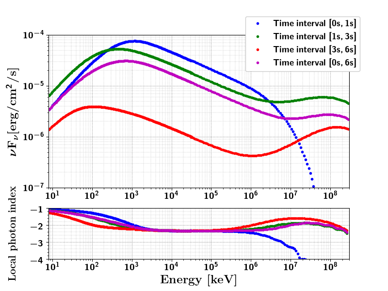
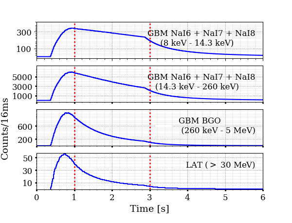
Figure 1: Left: Spectral energy distributions of the synthetic burst $\mathrm{GRB}$_$\mathrm{B010}$ and local photon index in the four time intervals [0 s, 1 s], [1 s, 3 s], [3 s, 6 s] and [0 s, 6 s]. Right: Multi-detector light curves of $\mathrm{GRB}$_$\mathrm{B010}$: summed counts in two energy ranges of GBM/NaI detectors (first two panels), in the GBM/BGO energy range (third panel) and using the largest LAT energy range (¿ 30 MeV) (bottom panel). The red dashed lines show the boundaries of the three time intervals [0 s, 1 s], [1 s, 3 s] and [3 s, 6 s].

3 Spectral models

The GRB spectra that we analyzed were fitted with several phenomenological functions that are commonly found in the literature, and with a new parametric function that is built from the synthetic spectra. All of the functions presented below are normalized by an amplitude parameter $A$, in units of cm^-2 s^-1 keV^-1.

3.1 Phenomenological models

3.1.1 Band function

The Band function (Band et al., 1993) is often used to fit the keV-MeV spectrum of GRBs. It is composed of two smoothly-connected power laws with four parameters $A_{\texttt{Band}}$, $\alpha$, $\beta$ and $E_{p}$, and it is defined as:

$$\frac{dN_{\texttt{Band}}}{dE}(E)=A_{\texttt{Band}}\left\{\begin{array}[]{l l}\left(\frac{E}{100\,\mathrm{keV}}\right)^{\alpha}\exp[-\frac{E\,(2+\alpha)}{E_{p}}],&E\leq E_{b}=E_{p}{{\alpha-\beta}\over{2+\alpha}}\\ \\ \left(\frac{E}{100\,\mathrm{keV}}\right)^{\beta}\left[\frac{E_{p}}{100\,\mathrm{keV}}\frac{\alpha-\beta}{2+\alpha}\right]^{\alpha-\beta}\exp[\beta-\alpha],&E>E_{b}=E_{p}{{\alpha-\beta}\over{2+\alpha}}.\end{array}\right.$$ (2)

The local photon index of this function reads:

$$\Gamma_{\texttt{Band}}(E)=\left\{\begin{array}[]{l l}\alpha-\frac{(2+\alpha)}{E_{p}}E,&E\leq E_{b}\\ \beta,&E>E_{b}.\end{array}\right.$$ (3)

3.1.2 Logarithmic parabola and variants

The log-parabola function (LP hereafter) has three free parameters, i.e. one less than the Band function. It was suggested by (Massaro et al., 2010) to fit GRB spectra and it is expressed as:

$$\frac{dN_{\texttt{LP}}}{dE}(E)=A_{\texttt{LP}}\left(\frac{E}{E_{0}}\right)^{-\gamma-\beta\log(E/E_{0})}$$ (4)

where $E_{0}$ is a fixed reference energy. The local photon index is a function of the spectral parameters $\gamma$ and $\beta$:

$$\Gamma_{\texttt{LP}}(E)=-\gamma-2\beta\log\left(\frac{E}{E_{0}}\right)$$ (5)

and the LP peak energy is $\displaystyle E_{p}=E_{0}\times 10^{\frac{2-\gamma}{2\beta}}$. The LP function is characterized by its continuous curvature, unlike the Band function. Its symmetric shape implies that the spectral parameter reconstruction is driven by the low-energy data, where most of the photon statistics is recorded. In order to gain some latitude at high energies, we modified the function to freeze the local photon index above a break energy $E_{b}$. As a result, the modified logarithmic parabola, denoted by LP1 hereafter, has four free parameters:

$$\frac{dN_{\texttt{LP1}}}{dE}(E)=A_{\texttt{LP1}}\left\{\begin{array}[]{l l}\left(\frac{E}{E_{0}}\right)^{-\gamma-\beta\,\log(E/E_{0})},&E\leq E_{b}\\ \left(\frac{E_{b}}{E_{0}}\right)^{-\gamma-\beta\,\log(E_{b}/E_{0})}\times\left(\frac{E}{E_{b}}\right)^{-\gamma-2\,\beta\,\log(E_{b}/E_{0})},&E>E_{b}\end{array}\right.$$ (6)

We introduced a similar modification at low energies, which relaxes the dependency of the spectral fit around the peak energy on the low-energy data. The corresponding modified logarithmic parabola, denoted by LP2 hereafter, has five free parameters:

$$\frac{dN_{\texttt{LP2}}}{dE}(E)=A_{\texttt{LP2}}\left\{\begin{array}[]{l l}\left(\frac{E_{b}^{\prime}}{E_{0}}\right)^{-\gamma-\beta\,\log(E_{b}^{\prime}/E_{0})}\times\left(\frac{E}{E_{b}^{\prime}}\right)^{-\gamma-2\,\beta\,\log(E_{b}^{\prime}/E_{0})},&E\leq E_{b}^{\prime}\\ \left(\frac{E}{E_{0}}\right)^{-\gamma-\beta\,\log(E/E_{0})},&E_{b}^{\prime}\leq E\leq E_{b}\\ \left(\frac{E_{b}}{E_{0}}\right)^{-\gamma-\beta\,\log(E_{b}/E_{0})}\times\left(\frac{E}{E_{b}}\right)^{-\gamma-2\,\beta\,\log(E_{b}/E_{0})},&E>E_{b}\end{array}\right.$$ (7)

3.1.3 (Broken) power law with exponential cutoff

For the spectral analysis of GRB 090926A presented in Sect. 6, which extends to the LAT energy range, we adopted either a power law with exponential cutoff (CUTPL) or a broken power law with exponential cutoff (CUTBPL). The CUTPL function is expressed as:

$$\frac{dN_{\texttt{CUTPL}}}{dE}(E)=A_{\texttt{CUTPL}}\left(\frac{E}{E_{0}}\right)^{\lambda}\exp\left(-\frac{E}{E_{f}}\right)$$ (8)

which has three free parameters $A_{\texttt{CUTPL}}$, $\lambda$ and the folding energy $E_{f}$ of the exponential cutoff, and a fixed reference energy $E_{0}$. The CUTBPL function is expressed as:

$$\frac{dN_{\texttt{CUTBPL}}}{dE}(E)=A_{\texttt{CUTBPL}}\left\{\begin{array}[]{l l}\left(\frac{E}{E_{0}}\right)^{\gamma_{0}}\exp\left(-\frac{E}{E_{f}}\right),&E\leq E_{b}\\ \\ \left(\frac{E_{b}}{E_{0}}\right)^{\gamma_{0}}\left(\frac{E}{E_{b}}\right)^{\gamma}\exp\left(-\frac{E}{E_{f}}\right),&E>E_{b}\end{array}\right.$$ (9)

where $E_{b}$ is the break energy, $\gamma_{0}$ and $\gamma$ are the photon index below and above $E_{b}$, respectively. As explained in Y17, the break energy and the photon spectral index below the break have been fixed to $E_{b}=200$ keV and $\gamma_{0}=+4$ in order to cancel the contribution of the power-law component at low energies, as for instance expected from an inverse Compton spectral component that would extend the synchrotron spectrum at high energies only. As a result, the CUTBPL function has the same number of free parameters as the CUTPL function.

3.2 The ISSM spectral model

In order to build a function that is representative of the synchrotron spectral component of the synthetic bursts, we fitted their local photon index as a function of energy with the following parameterization:

$$\Gamma(E)=\frac{\partial\ln(F)}{\partial\ln(E)}=-a+\frac{b}{E+c}$$ (10)

where $a$, $b$, $c$ are free parameters. This parameterization adequately fits the local photon index of $\mathrm{GRB}$_$\mathrm{B001}$ in the four time intervals as shown in the left panel of Fig. 2. The right panel of this figure shows that it is also suitable for different configurations of the model presented in BD14. Note that the synthetic bursts using various assumptions for the microphysics in the emission region do not have the same low-energy photon index: $\sim-1.5$ for case A as expected for the standard fast cooling synchrotron spectrum, and $-1.1$ to $-0.75$ for case B. Integrating Eq. 10, one gets:

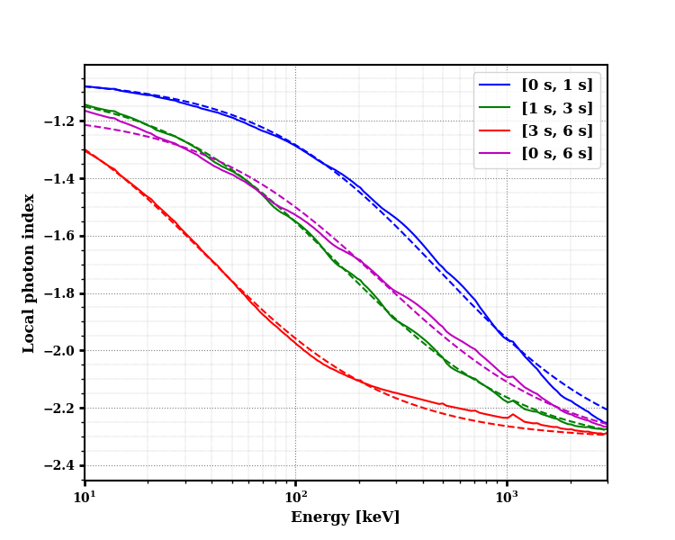
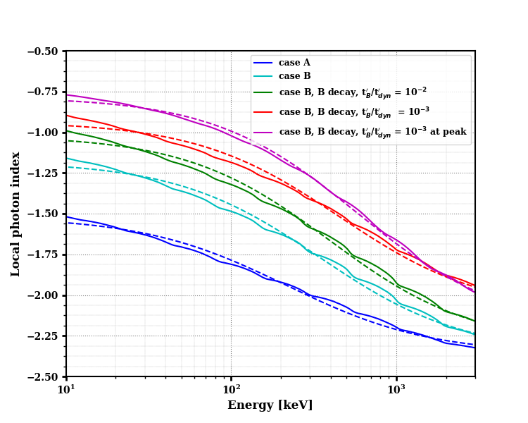
Figure 2: Left: Least-square fit (dashed lines) of Eq. 10 to the local photon index (thick lines) in the keV-MeV range for the four time intervals of the synthetic burst $\mathrm{GRB}$_$\mathrm{B001}$. Right: Least-square fit (dashed line) to the local photon index (solid line) in the keV-MeV range for several synthetic bursts: time integrated spectrum of two reference cases presented in BD14, case A (blue) and B (cyan) with a varying fraction of accelerated electrons and $p=2.7$. Case A corresponds to the most standard fast cooling synchrotron spectrum, and case B to a modified synchrotron spectrum affected by inverse Compton scaterring in the Klein-Nishina regime. In addition, preliminary calculation of the same case B taking into account a magnetic field decay in the emission region are also presented (taken from Daigne & Bošnjak, in preparation) with a time scale of the decay $t’_{\mathrm{B}}/t’_{\mathrm{dyn}}=10^{-2}$ (green) or $10^{-3}$ (red), where $t’_{\mathrm{dyn}}$ is the dynamical timescale. Finally, the same case is also shown for a time interval of $0.25\,\mathrm{s}$ around the peak of the light curve (magenta).

$$F(E)=F(E_{r})\exp\left[-a\ln\left(\frac{E}{E_{r}}\right)\right]\exp\left[\frac{b}{c}\ln\left(\frac{E\,(E_{r}+c)}{E_{r}\,(E+c)}\right)\right]$$ (11)

where the reference energy $E_{r}$ is related to the constant of integration. From this parameterization, the asymptotic spectral indices towards low and high energies can be easily obtained as $\alpha$= $\frac{b}{c}-a$ and $\beta=-a$, respectively. Finally, defining the SED peak energy $E_{p}$ as the solution of $\Gamma(E)=-2$:

$$E_{p}=-c\left(\frac{2+\alpha}{2+\beta}\right),$$ (12)

one can rewrite Eq. 11 to obtain a new expression, denoted by ISSM hereafter:

$$\frac{dN_{\texttt{ISSM}}}{dE}(E)=\frac{A_{\texttt{ISSM}}}{\left[1-\frac{E_{p}}{E_{r}}\left(\frac{2+\beta}{2+\alpha}\right)\right]^{\beta-\alpha}}\times\left(\frac{E}{E_{r}}\right)^{\alpha}\left[\frac{E}{E_{r}}-\frac{E_{p}}{E_{r}}\left(\frac{2+\beta}{2+\alpha}\right)\right]^{\beta-\alpha}$$ (13)

which has four parameters $A_{\texttt{ISSM}}$, $\alpha$, $\beta$, $E_{p}$. It is important to note that $E_{r}$ is a fixed reference energy which is chosen as the energy at which the flux normalization is defined:

$$\frac{dN_{\texttt{ISSM}}}{dE}(E_{r})=A_{\texttt{ISSM}}.$$ (14)

In other words, different choices of $E_{r}$ only affect the flux normalization parameter $A_{\texttt{ISSM}}$ and not the shape of the ISSM function. The local photon index is given by:

$$\Gamma_{\mathrm{\texttt{ISSM}}}(E)=\alpha+(\beta-\alpha)\frac{E}{E-E_{p}\left(\frac{2+\beta}{2+\alpha}\right)}.$$ (15)

The four parameters of the ISSM (flux normalization, SED peak energy and asymptotic slopes) resemble those of the Band function. The local photon index $\Gamma_{\mathrm{\texttt{ISSM}}}(E)$ decreases continuously with energy and the ISSM function is continuously curved unlike the Band function, and unlike simplified versions of the synchrotron model based on pure power-law energy distributions of the accelerated electrons. In the framework of our internal shock synchrotron model, the spectral curvature arises essentially from the superposition of instantaneous electron synchrotron spectra which vary significantly within the time intervals considered by the observer, owing to the dynamical evolution in the shock region. While we only tested the ISSM function on a simple, single-pulse burst, we are confident that it can also represent complex burst spectra resulting from various distributions of the Lorentz factor. Indeed, in most cases, complex bursts can be interpreted in terms of a succession of individual pulses so that time-dependent spectra of complex bursts can likely be fitted in the same way. Moreover, BD14 actually explored in detail how the observed emission of a single pulse depends on the various physical parameters of the internal shock model. Their study shows that the assumptions about the dynamics (Lorentz factor, kinetic energy flux, etc.) affect the pulse light curve but have little effect on the shape of the spectrum.

4 Spectral analysis of the synthetic bursts

We first focused our study of the three synthetic bursts in the GBM energy range (8 keV to 40 MeV). The four phenomenological functions and the ISSM function were used to fit the spectra of the synthetic bursts in the four time intervals [0 s, 1 s], [1 s, 3 s], [3 s, 6 s] and [0 s, 6 s] using the XSPEC software. The reference energy $E_{0}$ in Eqs. 4, 6 and 7 was fixed to $500$ keV. For simplicity, the reference energy in Eq. 13, which relates to the flux normalization, was fixed to the true peak energy of the synthetic spectra: $E_{r}$ = $1150$, $478$, $114$ and $745$ keV for the time intervals [0 s, 1 s], [1 s, 3 s], [3 s, 6 s] and [0 s, 6 s], respectively. To compare the quality of the fits between the different functions, we defined the following quality factor $Q$ that mimicks a reduced $\chi^{2}$:

$$Q=\frac{1}{n-n_{\mathrm{par}}}\sum\limits_{i=1}^{n}\left(\frac{\Gamma(E_{i})-s(E_{i})}{\sigma_{i}}\right)^{2}$$ (16)

where $\Gamma(E_{i})$ is the local photon index of the fitted function and $s(E_{i})$ is the true index of the synthetic spectrum at energy $E_{i}$. The error $\sigma_{i}$ on $\Gamma(E_{i})$ is obtained by propagating the errors of the $n_{\mathrm{par}}$ fitted function parameters.

Table 1: $C_{\mathrm{stat}}$ values of the spectral fits of the three synthetic bursts, performed with the five functions: Band, LP, LP1, LP2 and ISSM.

Synthetic GRB	Model	DOF	$C_{\mathrm{stat}}$ for time intervals:
			[0-1] s	[1-3] s	[3-6] s	[0-6] s
$\mathrm{GRB}$_$\mathrm{B001}$	Band	473	603	906	486	1403
	LP	474	768	677	615	631
	LP1	473	768	569	615	589
	LP2	472	526	540	558	570
	ISSM	473	486	498	452	638
$\mathrm{GRB}$_$\mathrm{B010}$	Band	473	458	539	447	578
	LP	474	470	559	455	469
	LP1	473	470	534	455	469
	LP2	472	439	525	455	466
	ISSM	473	441	523	443	484
$\mathrm{GRB}$_$\mathrm{B100}$	Band	473	465	446	359	461
	LP	474	464	445	364	447
	LP1	473	464	445	364	447
	LP2	472	462	442	376	447
	ISSM	473	463	444	360	449

The spectral analyses were performed using the Castor fit statistic ($C_{\mathrm{stat}}$) for Poisson distributed total counts of the burst. The $C_{\mathrm{stat}}$ values obtained from the fits of the three synthetic burst spectra are reported in Table 1. The ISSM function has the lowest $C_{\mathrm{stat}}$ value in most of the time intervals especially for the synthetic burst with the highest flux value i.e. $\mathrm{GRB}$_$\mathrm{B001}$. For $\mathrm{GRB}$_$\mathrm{B100}$, all functions yield similar $C_{\mathrm{stat}}$ values, meaning that the fits are of similar quality owing to the low photon statistics for this faint burst. Fig. 3 shows the SEDs and local photon index of the $\mathrm{GRB}$_$\mathrm{B010}$ burst in the time interval [1 s, 3 s], as obtained from the fits with the five spectral functions. As can be seen from this figure, both the SED and the local photon index are not reproduced by the Band function fit, in particular around and above the peak energy. The fit quality of the LP function is even worse owing to the linear dependency of its local photon index with energy, which is not adequate at low and high energies. The LP1 and LP2 functions provide better fits and their parameters are not constrained for the three bursts in all the time intervals. Finally, Fig. 3 shows that the ISSM function has the lowest $Q$ value among all fitted functions, which is expected from this model that has been built directly from the synthetic spectra.

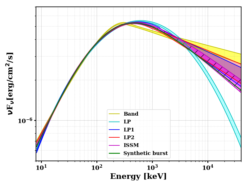
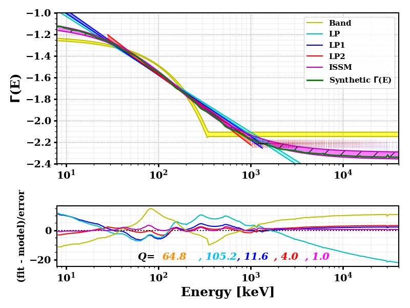
Figure 3: Left: SEDs of the $\mathrm{GRB}$_$\mathrm{B010}$ synthetic burst in the time interval [1 s, 3 s], from fits with the five spectral functions. The fit with the ISSM function is presented by the hatched magenta line. Right: Local photon index as a function of the photon energy. The fit quality factor $Q$ of the five functions is given in the bottom panel.

By nature, the ISSM function reproduces the keV-MeV spectra of the synthetic bursts simulated with the internal shock synchrotron model. It has the same number of free parameters as the Band function, which is commonly used to fit the prompt high-energy spectrum of GRBs. Therefore, before applying these functions to real GRB observations (see Sect. 5), it is worth comparing their shapes in detail. Tables 5, 6, and 7 in appendix show the parameters of the Band and ISSM fits to $\mathrm{GRB}$_$\mathrm{B001}$, $\mathrm{GRB}$_$\mathrm{B010}$ and $\mathrm{GRB}$_$\mathrm{B100}$, respectively. The asymptotic low-energy index $\alpha$ of the ISSM function is found to be larger than that of the Band function, while the high-energy index $\beta$ is smaller. Interestingly, the peak energies of the synthetic bursts are estimated with much greater accuracy with the ISSM function than with the Band function, which underestimates them by $\sim$36$\%$. Furthermore, we compared the spectral width of the two functions, following Yu et al. (2015) who proposed a method to calculate the SED sharpness around its peak energy. We did not consider the alternate measure of the spectral width proposed by Axelsson & Borgonovo (2015), which is defined as $W=\log(E_{2}/E_{1})$ where $E_{1}$ and $E_{2}$ are the energy bounds of the SED full width at half maximum. The spectral sharpness angle defined by Yu et al. (2015) is computed from the triangle defined by the vertices at $E_{p}/10$, $E_{p}$ and $3E_{p}$. To compute this angle and its asymmetrical errors accurately, we performed Monte-Carlo simulations using the fit parameters and their covariance matrix, assuming that their distribution is a multivariate Gaussian. This process was repeated $1000$ times for each time interval and for each of the two bright synthetic bursts $\mathrm{GRB}$_$\mathrm{B001}$ and $\mathrm{GRB}$_$\mathrm{B010}$. The spectral sharpness angle was chosen as the maximum probability value (MPV) of the distribution obtained from the $1000$ realizations. The errors on the angle were calculated from the $68$% confidence intervals on each side of the MPV. The results of this analysis are reported in Table 2, which confirms that the ISSM function reproduces the spectral width of the synthetic bursts better than the Band function.

Table 2: Spectral sharpness angle (in degrees) from the Band and ISSM fits to the synthetic bursts $\mathrm{GRB}$_$\mathrm{B001}$ and $\mathrm{GRB}$_$\mathrm{B010}$.

Synthetic GRB	Model	Time interval
		[0-1] s	[1-3] s	[3-6] s	[0-6] s
$\mathrm{GRB}$_$\mathrm{B001}$	Synthetic	142.3	145.9	145.5	148.9
	Band	137.7${}_{-0.2}^{+0.4}$	140.0${}_{-0.1}^{+0.2}$	142.7${}_{-0.3}^{+0.6}$	142.0${}_{-0.1}^{+0.2}$
	ISSM	143.5${}_{-0.5}^{+0.5}$	145.7${}_{-0.3}^{+0.3}$	145.8${}_{-1.0}^{+1.3}$	148.6${}_{-0.3}^{+0.4}$
$\mathrm{GRB}$_$\mathrm{B010}$	Synthetic	142.3	145.9	145.5	148.9
	Band	139.1${}_{-1.2}^{+0.9}$	139.9${}_{-0.4}^{+0.7}$	145.1${}_{-1.4}^{+1.8}$	142.6${}_{-0.6}^{+0.4}$
	ISSM	143.6${}_{-1.3}^{+1.8}$	146.5${}_{-1.2}^{+1.1}$	150.6${}_{-4.7}^{+4.7}$	148.9${}_{-0.8}^{+1.3}$

For the sake of completeness, we carried out broadband spectral analyses of the brightest synthetic burst ($\mathrm{GRB}$_$\mathrm{B001}$) in the two time intervals [1 s - 3 s] and [3 s - 6 s], where the inverse Compton spectral component is prominent. We used the CUTPL model to fit this high-energy spectral component and fixed the reference energy $E_{0}$ to $10$ GeV in Eq. 8. This value is close to the decorrelation energy and thus minimizes the correlation between the CUTPL parameters. Despite its brightness in the LAT energy range, the inverse Compton component of $\mathrm{GRB}$_$\mathrm{B001}$ peaks at $\sim 100$ GeV, where few simulated events are recorded. We multiplied artificially the LAT effective detection area by $100$ to get rid of these statistical limitations and to check whether the adopted model is able to capture all features in the internal shock model spectra. The fit results obtained with the ISSM + CUTPL model in the two time intervals are reported in Table 3 and shown in the left panel of Fig. 4 for the time interval [1 s - 3 s]. The fit residuals and reduced $C_{\mathrm{stat}}$ values clearly show the excellent quality of the fits and the ability of the ISSM + CUTPL model to reproduce the broadband shape of the synthetic spectra.

Table 3: Results of the ISSM +CUTPL fits to the synthetic burst $\mathrm{GRB}$_$\mathrm{B001}$ during the time intervals [1 s - 3 s] and [3 s - 6 s].

Spectral	Fit results	Time interval
component		[1-3] s	[3-6] s
ISSM	$E_{p}$ (keV)	458 $\pm$ 4	119 $\pm$ 3
	$\alpha$	-1.09 $\pm$ 0.01	-1.03 $\pm$ 0.05
	$\beta$	-2.354 $\pm$ 0.003	-2.321 $\pm$ 0.004
	AMeV (keV-1 cm-2 s-1)	0.145 $\pm$ 0.001	0.193 $\pm$ 0.001
CUTPL	$\lambda$	-1.51 $\pm$ 0.06	-1.28 $\pm$ 0.07
	Ef (GeV)	165 $\pm$ 71	172 $\pm$ 91
	AGeV (keV-1 cm-2 s-1)	(167.4 $\pm$ 11.5)$\times$10-13	(39.0 $\pm$ 3.5)$\times$10-13
ISSM + CUTPL	$C_{\mathrm{stat}}$/DOF	533/510	502/510

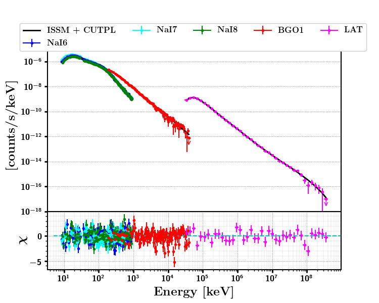
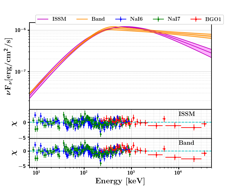
Figure 4: Left: Fit of the count spectrum of the synthetic burst $\mathrm{GRB}$_$\mathrm{B001}$ with the ISSM + CUTPL model in the time interval [1 s - 3 s]. Right: Fit of the ISSM and Band models to the GRB 150403913 spectrum oberved by the GBM.

5 Application to GBM bursts

5.1 GRB sample and data selection

According to the results presented in Sect. 4, a large number of counts is required to distinguish the different spectral model based on their fit quality. For this reason, we selected a sample of bursts detected by the GBM with an energy fluence larger than $10^{-5}$ erg cm^-2 (from 10 to 1000 keV), namely comparable to those of the $\mathrm{GRB}$_$\mathrm{B001}$ and $\mathrm{GRB}$_$\mathrm{B010}$ synthetic bursts. Like in Sect. 4, we first focused our study on the sub-MeV spectral component, discarding the bursts that have additional components at low or high energies. This includes the GRBs with a low-energy excess that has been interpreted as a possible thermal component (GRB 090424, GRB 090820 (Tierney et al., 2013), GRB 090902B (Abdo et al., 2009), GRB 090926A (Guiriec et al., 2015), GRB 100724B (Guiriec et al., 2011), GRB 110721 (Axelsson et al., 2012)), the GRBs with an extra high-energy power-law component (GRB 080916C (Ackermann et al., 2013), GRB 090902B (Abdo et al., 2009), GRB 090926A (Ackermann et al., 2011)) or with a strong spectral evolution (GRB 081215A (Tierney et al., 2013)). The bursts whose spectra are best fitted by a simple power law in the GBM spectral catalog (Gruber et al., 2014) were also excluded. Beside these 15 GRBs, we eliminated the bursts which have been seen by NaI detectors with a separation angle between the detector axis and the source larger than $60^{\circ}$. As a result, we selected $74$ GBM GRBs in the first eight observing years, which are listed in Table LABEL:tab:catalog:Band_IAP in appendix. More than half of them ($41$) are best fitted by the Band function in the GBM spectral catalog (Gruber et al., 2014). Another fair fraction of bursts from this catalog ($24$) are best fitted by a power law with an exponential cutoff. This model is a special case of the Band function that is obtained for a very steep high-energy index (i.e., $\beta$ tends to $-\infty$ and $E_{b}$ to $+\infty$ in Eq. 2). The remaining $9$ GRBs were found to be best fitted by a smoothly broken power law by Gruber et al. (2014), which is characterized by a flexible SED width around its peak energy. The data are loaded from the FSSC GBM data using gtburst tool . The spectral analyses where performed during the T90 defined in GBM catalog Gruber et al. (2014). For each GRB of the sample, we selected one BGO detector with a separation angle less than $90^{\circ}$ and a maximum of three NaI detectors that have seen the burst with a separation angle less than $60^{\circ}$.

5.2 Model comparison

We performed a spectral analysis of the $74$ selected GRBs with the XSPEC software and for the five spectral models: Band, LP, LP1, LP2 and ISSM. The reference energies $E_{0}$ in Eqs. 4, 6, 7 and $E_{r}$ in Eq. 13 of the LP, LP1, LP2 and ISSM functions, were fixed to $500$ keV. We used the “Poisson-Gauss” fit statistic ($PG_{\mathrm{stat}}$ hereafter), which is suitable for GRB spectral analysis, where the observed data counts are Poisson distributed in the energy channels, while background counts have been estimated beforehand from pre- and post-burst data and are assumed to follow a Gaussian distribution. The case of GRB 150403913 is shown in the right panel of Fig. 4 for the ISSM and Band fits. The left panel of Fig. 5 shows the increase of $PG_{\mathrm{stat}}$ of the five models with respect to the model which has the lowest $PG_{\mathrm{stat}}$ (“reference model” hereafter). In this panel, the GRBs are displayed in order of increasing signal-to-noise ratio (SNR), which is defined for each GRB as:

$$\mathrm{SNR}=\sum\limits_{i=1}^{N}(c_{i}-b_{i})\,/\sqrt{\sum\limits_{i=1}^{N}b_{i}}$$ (17)

where $c_{i}$ (resp. $b_{i}$) are the total (resp. background) counts recorded by the $N$ NaI detectors that have detected the burst. The right panel of Fig. 5 shows the resulting distribution of $\Delta$$PG_{\mathrm{stat}}$ for the five models. The ISSM function has the lowest $PG_{\mathrm{stat}}$, namely it is the reference model, for half of the GRBs in Fig. 5. Since the ISSM function shows the lowest value of $PG_{\mathrm{stat}}$ in half of the cases, it is taken as a reference (level 0 on the bottom of Fig. 5) and the other models are displayed accordingly. The first GRBs with the minimum SNR values in this figure have comparable $PG_{\mathrm{stat}}$ values for the five spectral models and the $\Delta$$PG_{\mathrm{stat}}$ increases with SNR as expected, since the models can be more easily distinguished from each other with a larger event statistics.

To compare the fitted models with each other, we used the $\Delta$$PG_{\mathrm{stat}}$ as a likelihood ratio test (Neyman & Pearson, 1928). In case of nested models, where the model parameterization in the null hypothesis is a special case of that in the alternative hypothesis, the $\Delta$$PG_{\mathrm{stat}}$ is expected to follow a $\chi^{2}$ distribution with $k$ degrees of freedom in the large sample limit, where $k$ is the number of additional parameters between the two models (Wilks, 1938). Since several of the models that we considered are not nested, and because the large sample limit is not reached in all energy channels of the GRBs in our sample, one should compute the $\Delta$$PG_{\mathrm{stat}}$ probability density function for each GRB and each pair of models by simulating a large number of spectra. Given the vast number of cases, we focused on the Band and ISSM functions, in the two cases of a low or a medium value of the SNR. We performed Monte-Carlo simulations for two cases in our sample, GRB 100910A (SNR=141) and GRB 110921A (SNR=249), considering the Band function as the null hypothesis. We used the XSPEC software to simulate 10⁵ Band spectra for the duration of each GRB, using the DRM and background files of the GBM detectors that have seen the burst with the best viewing angle. All the simulated spectra were then fitted with the Band and ISSM functions. The resulting distribution of $\Delta PG_{\mathrm{stat}}=PG_{\mathrm{stat},\texttt{Band}}-PG_{\mathrm{stat},\texttt{ISSM}}$ for GRB 110921A is shown in the left panel of Fig. 6. The fit of this distribution with an asymmetric Gaussian function and its extrapolation allowed us to compute the $\Delta$$PG_{\mathrm{stat}}$ limit beyond which the probability that a statistical fluctuation yields a better fit with the ISSM function than with the Band function is smaller than $10^{-6}$ (approximately $5$ Gaussian standard deviations). The limit was found to be $\Delta$$PG_{\mathrm{stat}}$ $=20$ for a low SNR and $3$ for a medium SNR, beyond which the null hypothesis (i.e., the Band function) must be rejected. Because it was complicated and time consuming to determine a limit for each GRB and each pair of models, we adopted a common limit of $\Delta$$PG_{\mathrm{stat}}$ $=10$ in all situations.

As a result, this study revealed that the ISSM model is the reference model for $36$ GRBs, $19$ of which are equivalently fitted by the Band function. On the contrary, the Band function has the lowest $PG_{\mathrm{stat}}$ value for $16$ GRBs, $10$ of which are equivalently fitted by the ISSM function. Concerning the other three models, only the LP2 showed good performance. It is the reference model for $18$ GRBs, and globally as good as the Band model, though with one more parameter. All in all, the ISSM function is a good spectral model for $81$% ($60/74$) of the GRBs in our sample, namely in these cases it is the reference model or it is close enough to it in terms of $PG_{\mathrm{stat}}$. The Band function was found to be a good spectral model for a smaller fraction ($59$%) of the GRB sample ($44/74$), similar to the LP2 function ($65$%), versus only $\sim$$20$% for the LP1 and LP functions. It must be noted that these performances would improve for more common and less fluent bursts with lower signal-to-noise ratios.

Figure 5: Left: Difference in $PG_{\mathrm{stat}}$ of the five models with respect to the model with the lowest $PG_{\mathrm{stat}}$, for every GRB displayed with increasing SNR (increasing from the left to the right). For each GRB, the five model markers are displayed within two vertical (red and blue) lines. By definition, the model with the lowest $PG_{\mathrm{stat}}$ is always placed on the zero horizontal line. Lower limits at the top of the figure stand for models with a $\Delta$$PG_{\mathrm{stat}}$ larger than $100$. Right: Distribution of $\Delta$$PG_{\mathrm{stat}}$ for the five models.

Figure 6: Left: Fit of an asymmetric Gaussian function to the distribution of $\Delta$$PG_{\mathrm{stat}}$ between the Band and the ISSM function for the medium SNR case. The bottom panel shows the ratio of the difference between the histogram and its fit over the error ($\sqrt{N}$ in each bin). Right: Spectral energy distribution and local photon index of a representative burst (GRB 150403913) with the Band and ISSM functions.

5.3 Band and ISSM spectral parameters

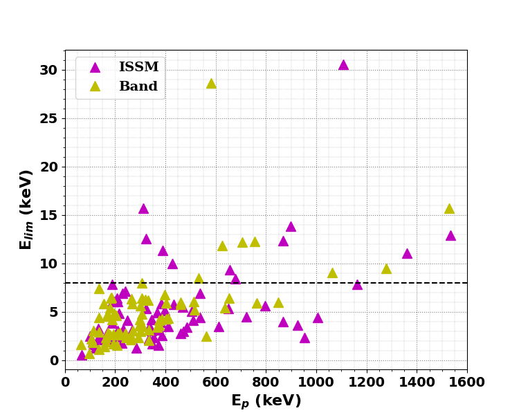
Figure 7: Left: Comparison of the $E_{p}$ parameter between the Band and ISSM functions. The dashed line is the equality line. The inset shows the ratio between the $E_{p}$ values obtained by ISSM and Band functions. Right: limit energies $E_{\mathrm{lim}}$ of the ISSM and Band functions compared with their peak energies $E_{p}$. The horizontal dashed line represents the lower limit of the GBM energy range.

In this section we compare the spectral parameters of the Band and ISSM functions. The left panel of Fig. 7 shows the SED peak energies obtained with the two models. The $E_{p}$ values of the ISSM function are found to be systematically larger than the values obtained with the Band function. The low-energy index $\alpha$ is an asymptotic value that is rarely reached by the local photon index within the energy range of any burst-observing instrument. For this reason, Preece et al. (1998) defined an effective low-energy index at the CGRO/BATSE detector lower limit ($25$ keV). In order to find the energy limit ($E_{\mathrm{lim}}$) at which the local photon index $\Gamma(E)$ approaches the asymptotic value $\alpha$ within its error $\delta\alpha$, we solved the equation $\Gamma(E_{\mathrm{lim}})=\alpha-\delta\alpha$ using the definition of the local photon index of the Band and ISSM functions in Eqs. 3 and 15, respectively. The $E_{\mathrm{lim}}$ energies of the two functions are expressed as:

$$E_{\mathrm{lim,\texttt{Band}}}=\frac{\delta\alpha}{2+\alpha}\,E_{p}$$ (18)

$$E_{\mathrm{lim,\texttt{ISSM}}}=\frac{\delta\alpha\,(2+\beta)}{(2+\alpha)(\beta-\alpha+\delta\alpha)}\,E_{p}$$ (19)

These quantities are displayed with respect to $E_{p}$ in the right panel of Fig. 7. For the vast majority of the GRBs in our sample, the $E_{\mathrm{lim}}$ values fall below the GBM energy range. We thus defined $\alpha_{10}$ as the local photon index at $10$ keV, namely right above the low-energy detection limit of the GBM. The left panel of Fig. 8 compares the $\alpha_{10}$ index to the $\alpha$ asymptotic index for both the Band and ISSM functions. While the $\alpha$ indices of the ISSM function are larger than those of the Band function, the $\alpha_{10}$ indices of the ISSM function are only slightly larger. The values of $\alpha_{10}$ appear also less scattered than those of $\alpha$. More interestingly, the fraction of GRBs that are fitted with the ISSM function and whose index is harder than the synchrotron slow-cooling limit ($-2/3$) decreases from $35$% ($\alpha$ asymptotic index) to $26$% ($\alpha_{10}$). This fraction decreases from $19$% to $12$% for the Band function. As shown in the right panel of Fig. 8 that displays the $\alpha$ and $\alpha_{10}$ distributions for both models, the weighted mean index of the ISSM (resp. Band) function indeed decreased from $\langle\alpha\rangle=-0.75$ (resp. $-0.88$) to $\langle\alpha_{10}\rangle=-0.97$ (resp. $-1.03$).

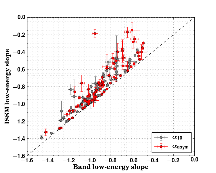
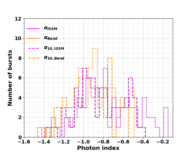
Figure 8: Left: Comparison of the asymptotic $\alpha$ and the local photon index $\alpha_{10}$ at 10 keV between the Band and ISSM functions. The gray dashed line denotes equality. The dashed-dotted horizontal and vertical lines indicate the upper limit ($-2/3$) of the low-energy spectral index for synchrotron emission in the slow cooling regime. Right: Distributions of the $\alpha$ and $\alpha_{10}$ parameters of the Band and ISSM functions.

Similarly, the $\beta$ parameter of the ISSM function is an asymptotic value at high energy, which may not be reached by the local photon index within the GBM energy range. Therefore, we defined $\beta_{b}$ as the photon index at the break energy $E_{b}$ of the Band function (Eq. 2). By definition, $\beta_{b}$ is equal to $\beta$ for the Band function, while is it harder than $\beta$ for the ISSM function owing to its continuous curvature. The $\beta_{b}$ index of the ISSM function was also found to be systematically harder than that of the Band function, namely $\beta_{\texttt{ISSM}}$ ¡ $\beta_{\texttt{Band}}$ ¡ $\beta_{b,\texttt{ISSM}}$. As a result, GRB spectra appear slightly wider around their peak energy when fitted with the ISSM function than with the Band function, but narrower when observed over a wider energy range. This is illustrated in the right panel of Fig. 6, for the case of GRB 150403913, which is best fitted by the ISSM model.

5.4 Band and ISSM spectral sharpness

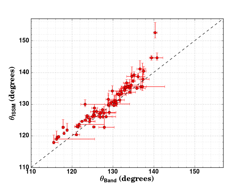
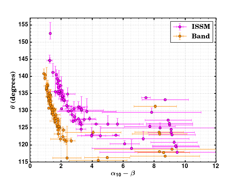
Figure 9: Left: Spectral sharpness angles of the ISSM fits versus the angles of the Band fits to the GRB spectra. Right: Spectral sharpness angle as function of the difference between the $\alpha_{10}$ and $\beta$ parameters for the Band and ISSM functions.

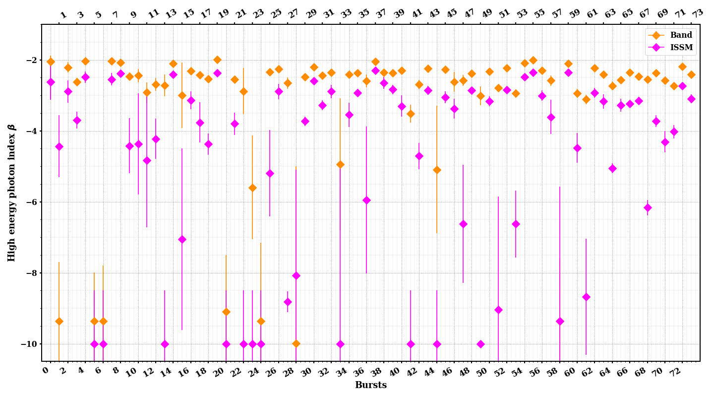
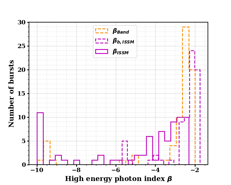
Figure 10: Left: Distribution of the high-energy index $\beta$ of the Band and ISSM functions. The lowest limit value used for $\beta$ was fixed to -10. Right: Distributions of the $\beta$ parameter of the Band and ISSM functions.

We investigated how the sharpness of the Band and ISSM fitted spectra varies quantitatively with the photon indices. Following the methodology described in Sect. 4, a set of $10^{3}$ spectra was simulated for each GRB using its fit parameters and their covariance matrix. The spectral sharpness angles of the GRB sample are presented in the left panel of Fig. 9. Similarly to the synthetic bursts analyzed in Sect. 4, the ISSM spectra are slightly wider than the Band spectra. As expected, the spectral sharpness angle was found to be independent of the peak energy, and to depend strongly on the photon indices. As shown in the right panel of Fig. 9, the spectral sharpness angle decreases with increasing $\alpha_{10}$ and/or with decreasing $\beta$. The spectral sharpness angles of the GRBs in our sample are similar to those obtained by Yu et al. (2015) (see figures therein, e.g., the blue solid curve in the left panel of Fig. 7), ranging from $\sim 115^{\circ}$ to $\sim 140^{\circ}$ in both analyses, except one with angle 152^∘ with the ISSM function.

More importantly, the spectral sharpness angle of the synthetic bursts fitted by the ISSM function is $149^{\circ}$ (see Table 2), which is larger than for any GRB in our sample using the same fitting model. This results essentially from the difference in the low-energy spectral index, $\alpha\simeq-1.2$, which is softer than for most of the analyzed GRBs (see the left panel of Fig. 8). Besides, the value of the high-energy index of the synthetic burst, $\beta\simeq-2.3$, is close to the higher bound of the sample distribution as shown in Fig. 10. Possible ways to improve the agreement between the synthetic and observed bursts will be discussed in Sect. 7.

6 Application to GRB 090926A

The prompt light curve of GRB 090926A shows a short and bright spike at $10$ s post-trigger which has been detected from keV to GeV energies by the Fermi instruments (Ackermann et al., 2011). This spike coincides with the emergence of a hard power-law spectral component which is attenuated at the highest energies. In Y17, we performed a dedicated analysis of the broadband prompt emission spectrum of GRB 090926A by combining the GBM data with the LAT Pass 8 data above $30$ MeV. Using a Band +CUTBPL fitting function, we showed that the spectral break energy increases with time, and that the entire prompt emission of this burst, namely the emission that is observed from keV to GeV energies by the GBM and the LAT during the GRB duration in the 50-300 keV energy band, can be interpreted as the result of synchrotron emission of shock-accelerated electrons in the keV-MeV domain, with an inverse Compton spectral component at higher energies. The latter component was fitted by the CUTBPL function instead of the CUTPL function to avoid any unrealistic contribution to the observed flux in the GBM low-energy range. As a result, the low-energy index $\alpha$ of the Band spectral component was found to be close to $-0.9$, which is in agreement with the theoretical index ($\sim-1$) of the fast-cooling synchrotron spectrum that is expected in the presence of inverse Compton scatterings in the Klein-Nishina regime (BD14).

Going further, we revisited the spectral analysis of GRB 090926A and compared the Band + CUTBPL model to the ISSM + CUTBPL model. This analysis was performed with the XSPEC software for the time intervals $c$ ($0.98$ s to $10.5$ s) and $d$ ($10.5$ s to $21.5$ s) where the high-energy break is detected. Following Y17, we fixed the parameters $\gamma_{0}$ and the break energy $E_{b}$ of Eq. 9 to $+4$ and $200$ keV, respectively. Like in Y17, the reference energy $E_{0}$ was fixed to $10$ MeV and $100$ MeV for the time intervals $c$ and $d$, respectively. The results of this analysis are presented in Fig. 11 and summarized in Table 4. As can be seen in all panels of this figure and from the $PG_{\mathrm{stat}}$ fit statistics, both the Band +CUTBPL and ISSM +CUTBPL models reproduce adequately the GRB spectrum, especially in the time interval $c$ (top panels). The low-energy indices $\alpha$ of the Band and ISSM spectral components are equal within statistical errors, and close to $-1$ and $-0.9$ for the time intervals $c$ and $d$, respectively. Again, these values perfectly agree with the predictions of BD14. All other spectral parameters are also equivalent between both models, except the high-energy index $\beta$ of the keV-MeV spectral component, which is not well constrained using the ISSM function. Since the ISSM flux decreases more rapidly than that of the Band function beyond the SED peak energy, this likely results from the lack of photon statistics in the SED dip at a few MeV, between the GBM and LAT energy domains.

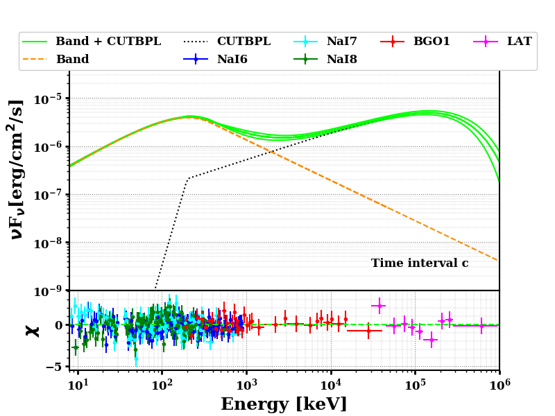
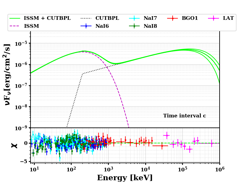
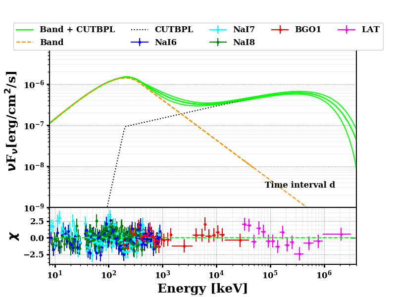
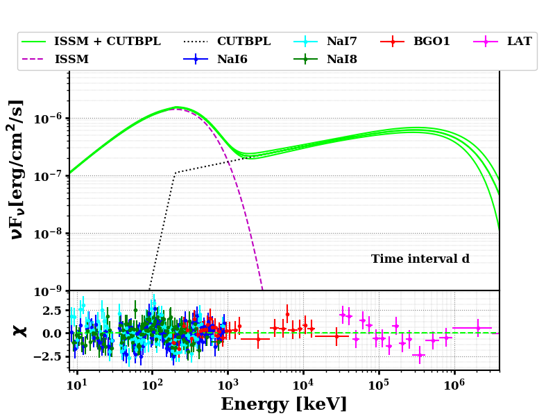
Figure 11: Spectral energy distributions of GRB 090926A in time intervals $c$ (top panels) and $d$ (lower panels) from the joint GBM/LAT analysis using LAT Pass 8 above $30$ MeV. The solid curve represents the Band + CUTBPL model (left colum) and the ISSM + CUTBPL model (right column), within a 68$\%$ confidence level contour derived from the errors on the fit parameters. The reference energy of the CUTBPL was fixed to $10$ MeV like in Y17.

Table 4: Results of the Band +CUTPL and ISSM +CUTBPL fits to GBM/LAT data in the time intervals $c$ and $d$ of GRB 090926A.

Time intervals	Parameters	Band + CUTBPL	ISSM + CUTBPL
[0.98 s -10.5 s]	$A_{\texttt{Band}/\texttt{ISSM}}$ (keV-1 cm-2 s-1)	$0.33_{-0.01}^{+0.02}$	$580_{-5}^{+5}$($\times 10^{-5}$)
	$E_{p}$ (keV)	$203_{-7}^{+7}$	$203_{-1}^{+1}$
	$\alpha$	$-0.98_{-0.03}^{+0.03}$	$-0.97_{-0.02}^{+0.02}$
	$\beta$	$-2.8_{-0.3}^{+0.2}$	$-14.0_{-1.0}^{+4.7}$
	$A_{\texttt{CUTBPL}}$ ($\times 10^{4}$ keV-1 cm-2 s-1)	$2.04_{-0.89}^{+1.37}$	$3.46_{-0.32}^{+0.22}$
	$\lambda$	$-1.43_{-0.11}^{+0.10}$	$-1.52_{-0.02}^{+0.02}$
	$E_{f}$ (GeV)	$0.25_{-0.05}^{+0.07}$	$0.27_{-0.05}^{+0.07}$
	$PG_{\mathrm{stat}}$/DOF	577/510	582/510
[10.5 s - 21.5 s]	$A_{\texttt{Band}/\texttt{ISSM}}$ (keV-1 cm-2 s-1)	$0.123_{-0.003}^{+0.003}$	$203_{-11}^{+16}$($\times 10^{-5}$)
	$E_{p}$ (keV)	$201_{-5}^{+5}$	$204_{-5}^{+7}$
	$\alpha$	$-0.88_{-0.02}^{+0.02}$	$-0.86_{-0.02}^{+0.02}$
	$\beta$	$-3.0_{-0.3}^{+0.1}$	$-14_{-1}^{+9}$
	$A_{\texttt{CUTBPL}}$ ($\times 10^{7}$ keV-1 cm-2 s-1)	$8.89_{-2.72}^{+2.92}$	$10.74_{-2.93}^{+1.65}$
	$\lambda$	$-1.70_{-0.05}^{+0.06}$	$-1.73_{-0.04}^{+0.05}$
	$E_{f}$ (GeV)	$1.08_{-0.25}^{+0.31}$	$1.12_{-0.25}^{+0.32}$
	$PG_{\mathrm{stat}}$/DOF	714/510	717/510

7 Discussion

Our analysis of a sample of $74$ GRBs that are bright and fluent in the GBM showed that the ISSM function adequately reproduces most ($81$%) of the keV-MeV prompt emission spectra, while the Band phenomenological function is suitable for a smaller fraction ($59$%). We observed noticeable differences between the spectra fitted with these two functions. The peak energies $E_{p}$ of the spectra that are reconstructed using the ISSM function are somewhat higher than those of the spectra resulting from the Band function fits. In addition, the ISSM fitted spectra are globally narrower than the Band fitted spectra, yet they appear slightly wider close to $E_{p}$. This results in slightly larger sharpness angles for the ISSM fitted spectra, which was also observed from fits of the synthetic spectrum.

Although the shape of the ISSM function seems adequate to reproduce the spectral curvature of the GBM bright bursts, the spectral sharpness angle in this sample is always smaller than the sharpness angle of the synthetic spectra that were used to build this fitting function. Since the spectral sharpness angle scales almost linearly with $\beta-\alpha$ (right panel of Fig. 9), it is worth investigating possible ways to improve the agreement between the data and the physical model. Firstly, the high-energy photon index $\beta$ in the model is strongly related to the slope of the electron power-law energy distribution $p$, as $\beta=-(p/2+1)$ in the synchrotron fast-cooling regime. While $p=2.7$ and thus $\beta=-2.3$ for the synthetic bursts, larger values of $p$ up to $2.9$ could be considered (BD14), owing to the theoretical uncertainties on the energy distribution of accelerated electrons in midly-relativistic shocks. However, the expected change in the value of $\beta$ would not entirely account for the sharpness discrepancy with observed spectra. Moreover, many of the observed values of $\beta$ are larger for the bursts with well-measured spectral parameters as shown in Fig. 10. In this figure, softer high-energy indices appear with larger uncertainties and might be underestimated due to insufficient photon statistics above the peak energy. This suggests that a better spectral coverage at MeV energies could result in harder values of $\beta$ and in larger sharpness angles for this fraction of the burst sample, making the entire sample compatible with the physical model.

Secondly, the low-energy photon index $\alpha$ of the synthetic spectra is close to $-1.2$. As shown in Fig. 9, an increase of $0.5$ in this theoretical slope, with a condition that the high-energy slope does not increase, would be enough to make the synthetic spectra compatible with the GBM sample in terms of spectral sharpness. As a matter of fact, harder values of $\alpha$ are expected from internal shock synchrotron models in the so-called marginally fast-cooling regime (Daigne et al., 2011; Beniamini & Piran, 2013), where the impact of adiabatic losses on the electron energy distribution is not negligible anymore as compared to the effect of radiative losses. In this regime, specific configurations of the jet such as low-contrast internal shocks can lead to $\alpha$ values as hard as $-2/3$ (Daigne et al., 2011). Hardening the low-energy part of the synchrotron spectrum could also be obtained by accounting for the decay of the magnetic field behind the shock (Pe’er & Zhang, 2006; Derishev, 2007). In such a configuration, the most energetic electrons would indeed explore a small region where the magnetic field has not decreased yet, while the less energetic electrons would see a less intense magnetic field on average. Therefore, such a magnetic field decay appears as a natural possibility to reach the marginally fast cooling regime without any need for a fine-tuning of the microphysical parameters (Daigne & Bošnjak, in preparation). Indeed, as the magnetic field decreases, the critical Lorentz factor of electrons for slow cooling $\gamma_{\mathrm{c}}$ increases.

Preliminary results show that a steep asymptotic slope $\alpha$ close to $-2/3$ is obtained. This effect of a magnetic field decay is shown in the right panel of Fig. 2 where the value of the ISSM low-energy slope $\alpha=b/c-a$ varies between $-1.5$ (case A with a constant magnetic field) and $-0.8$ (case B with a magnetic field decay for the spectrum measured at the peak of the light curve). This illustrates that a more realistic modeling of the microphysics in the acceleration and emission regions should be investigated to reach a full agreement between the synthetic and observed spectra. Ultimately one would like to use the spectral fits to infer the physical parameters of the model such as the evolution of the injected power or the distribution of the Lorentz factor in the flow. In practice, analysis of the spectra only provides values for the four parameters: $A_{\texttt{ISSM}}$, $\alpha$, $\beta$ and $E_{p}$. They partially constrain the shock physics and radiative mechanism as discussed above for $\alpha$ and $\beta$. The peak energy $E_{p}$ depends on a combination of the ejecta physical parameters and shock microphysics. It will therefore be difficult to decipher from the evolution of $E_{p}$ the form of the Lorentz factor or/and injected power distributions even if some general trends can probably be obtained. This will require a dedicated study.

8 Conclusions

The physical origin of GRB prompt emission remains elusive despite decades of observations. Characterizing the prompt emission spectra has been often performed using phenomenological parameterizations with little physical grounds, such as the Band function. However, the advance of instrument spectral coverage and the improved data quality provided by current missions such as the Fermi observatory now offer the possibility to confront observations to theoretical models in detail. In this work, we used the internal shock model developed by BD14 to produce synthetic GRBs (see also Bošnjak et al. (2009) and Daigne et al. (2011)), and we folded their spectra with the response of the Fermi GBM and LAT. The synthetic spectra obtained from these simulations in the keV-MeV domain, where the synchrotron emission is dominant, were used to build a new GRB spectral fitting function called ISSM, which has the same number of parameters as the Band function. We used the ISSM function to fit the prompt emission spectra for a sample of $74$ GBM fluent bursts, which improved the fit quality as compared to the phenomenological Band function in a sizeable number of cases. In addition, we combined the ISSM function with a CUTBPL spectral component to fit the GRB 090926A broadband spectrum with some success. This work was motivated by a previous study of this burst that suggested an internal origin of the keV to GeV emission observed during the prompt phase (Y17). In this framework, our interpretation of both spectral components as being from synchrotron and inverse Compton emissions would greatly benefit from a more realistic parameterization of the high-energy component based on the synthetic spectra, especially in the overlapping region at MeV energies.

The analysis of the GBM sample of $74$ bursts showed noticeable differences between the ISSM and Band fits. Peak energies and spectral sharpness angles that are obtained from the ISSM fits are slightly larger than those from the Band fits. This result can be attributed to the continuous curvature of the ISSM function. This curvature reflects the time evolution of the electron and photon energy distributions within the analysed time intervals, which lasts longer than the typical dynamical timescales in the physical model. While observed spectra can be well fitted by the ISSM physical function, they appear narrower than the synthetic spectra, essentially because of a theoretical low-energy photon index that differs significantly from the observed photon index $\alpha$. This problem clearly calls for improvements of the internal shock model and possible solutions have been identified. In particular, more sophisticated prescriptions for the jet physics should be investigated in the future, such as the marginally fast-cooling regime and the decay of the magnetic field behind the shocks. Inferring the parameters of the physical model from the fitted parameters of the ISSM function is not easy as their relation is complex. Actually, the physical parameters that best reproduce GRB prompt emission spectra should be rather explored by fitting the numerical model directly to the data in the future, without using the ISSM proxy function. On the experimental side, complementary multi-wavelength observations will be also performed by GRB-dedicated missions such as SVOM which will observe the complete time evolution of GRBs from possible precursors until the afterglow phase (Wei et al., 2016). SVOM will measure GRB prompt emission spectra down to $4$ keV thanks to its ECLAIRs coded-mask telescope, and up to the MeV range with its Gamma-Ray Monitor detector (Bernardini et al., 2017). This will provide more insight into the physical origin of GRB high-energy emission at early times.

Appendix A Spectral analysis results

Table 5: Results of the Band and ISSM fits for $\mathrm{GRB}$_$\mathrm{B001}$ in the four time intervals. The true peak energies are $E_{p,true}=1150$, $478$, $114$ and $745$ keV for the time intervals [0 s, 1 s], [1 s, 3 s], [3 s, 6 s] and [0 s, 6 s] respectively.

Time interval	Model	$E_{p}$	$E_{p}$/$E_{p,true}$	$\alpha$	$\beta$	Amplitude
					($\times 10^{-3}$ cm-2 s-1 keV-1)
[0 s, 1 s]	Band	761 $\pm$ 14	0.66	-1.14 $\pm$ 0.01	-2.16 $\pm$ 0.01	1962 $\pm$ 10
	ISSM	1216 $\pm$ 25	1.06	-1.07 $\pm$ 0.01	-2.45 $\pm$ 0.02	36 $\pm$ 1
[1 s, 3 s]	Band	295 $\pm$ 3	0.62	-1.22 $\pm$ 0.01	-2.13 $\pm$ 0.01	3100 $\pm$ 19
	ISSM	459 $\pm$ 6	0.96	-1.09 $\pm$ 0.01	-2.35 $\pm$ 0.01	145 $\pm$ 1
[3 s, 6 s]	Band	99 $\pm$ 3	0.87	-1.37 $\pm$ 0.02	-2.16 $\pm$ 0.01	477 $\pm$ 15
	ISSM	119 $\pm$ 3	1.04	-0.95 $\pm$ 0.08	-2.29 $\pm$ 0.02	192 $\pm$ 1
[0 s, 6 s]	Band	378 $\pm$ 4	0.51	-1.27 $\pm$ 0.01	-2.09 $\pm$ 0.01	1465 $\pm$ 6
	ISSM	659 $\pm$ 9	0.88	-1.16 $\pm$ 0.01	-2.28 $\pm$ 0.01	34 $\pm$ 1

Table 6: Results of the Band and ISSM fits for $\mathrm{GRB}$_$\mathrm{B010}$ in the four time intervals. The true peak energies are $E_{p,true}=1150$, $478$, $114$ and $745$ keV for the time intervals [0 s, 1 s], [1 s, 3 s], [3 s, 6 s] and [0 s, 6 s] respectively.

Time interval	Model	$E_{p}$	$E_{p}$/$E_{p,true}$	$\alpha$	$\beta$	Amplitude
					($\times 10^{-3}$ cm-2 s-1 keV-1)
[0 s, 1 s]	Band	677 $\pm$ 40	0.59	-1.13 $\pm$ 0.01	-2.11 $\pm$ 0.04	2008 $\pm$ 37
	ISSM	1178 $\pm$ 82	1.02	-1.06 $\pm$ 0.02	-2.41 $\pm$ 0.07	35 $\pm$ 1
[1 s, 3 s]	Band	298 $\pm$ 11	0.62	-1.23 $\pm$ 0.01	-2.13 $\pm$ 0.02	3077 $\pm$ 58
	ISSM	470 $\pm$ 18	0.98	-1.08 $\pm$ 0.03	-2.33 $\pm$ 0.03	145 $\pm$ 2
[3 s, 6 s]	Band	104 $\pm$ 11	0.91	-1.44 $\pm$ 0.05	-2.13 $\pm$ 0.03	424 $\pm$ 41
	ISSM	127 $\pm$ 11	1.11	-1.02 $\pm$ 0.27	-2.23 $\pm$ 0.05	187 $\pm$ 3
[0 s, 6 s]	Band	377 $\pm$ 13	0.51	-1.27 $\pm$ 0.01	-2.07 $\pm$ 0.02	1456 $\pm$ 20
	ISSM	685 $\pm$ 32	0.92	-1.16 $\pm$ 0.02	-2.26 $\pm$ 0.03	34 $\pm$ 1

Table 7: Results of the Band and ISSM fits for $\mathrm{GRB}$_$\mathrm{B100}$ in the four time intervals. The true peak energies are $E_{p,true}=1150$, $478$, $114$ and $745$ keV for the time intervals [0 s, 1 s], [1 s, 3 s], [3 s, 6 s] and [0 s, 6 s] respectively.

Time interval	Model	$E_{p}$	$E_{p}$/$E_{p,true}$	$\alpha$	$\beta$	Amplitude
					($\times 10^{-3}$ cm-2 s-1 keV-1)
[0 s, 1 s]	Band	709 $\pm$ 135	0.62	-1.09 $\pm$ 0.05	-2.07 $\pm$ 0.12	193 $\pm$ 11
	ISSM	1333 $\pm$ 324	1.16	-1.03 $\pm$ 0.08	-2.40 $\pm$ 0.24	4 $\pm$ 1
[1 s, 3 s]	Band	297 $\pm$ 37	0.62	-1.25 $\pm$ 0.04	-2.13 $\pm$ 0.07	301 $\pm$ 18
	ISSM	457 $\pm$ 50	0.96	-1.18 $\pm$ 0.07	-2.45 $\pm$ 0.16	14 $\pm$ 1
[3 s, 6 s]	Band	55 $\pm$ 17	0.48	-0.90 $\pm$ 0.38	-2.00 $\pm$ 0.06	136 $\pm$ 121
	ISSM	130 $\pm$ 34	1.14	unconstrained	-2.18 $\pm$ 0.13	19 $\pm$ 1
[0 s, 6 s]	Band	445 $\pm$ 50	0.60	-1.31 $\pm$ 0.03	-2.13 $\pm$ 0.07	137 $\pm$ 5
	ISSM	678 $\pm$ 78	0.91	-1.24 $\pm$ 0.04	-2.38 $\pm$ 0.12	3.5 $\pm$ 0.1

Table 8: Results of the Band and ISSM spectral fits to GBM data for the prompt emission of 74 GRBs. The amplitudes are given in units of $10^{-4}\,$cm^-2 s^-1 keV^-1.

GRB name	Models	$E_{p}$	$\alpha$	$\alpha_{10}$	$\beta$	$\beta_{b}$	Amplitude	$PG_{\mathrm{stat}}$/DOF
GRB080817161	Band	410 $\pm$ 14	-0.96 $\pm$ 0.01	-1.00 $\pm$ 0.01	-2.32 $\pm$ 0.08	-2.32 $\pm$ 0.08	145 $\pm$ 2	1031 / 469
	ISSM	509 $\pm$ 11	-0.88 $\pm$ 0.02	-0.93 $\pm$ 0.01	-3.13 $\pm$ 0.25	-2.03 $\pm$ 0.02	8.9 $\pm$ 0.2	1021 / 469
GRB080825593	Band	187 $\pm$ 7	-0.64 $\pm$ 0.03	-0.75 $\pm$ 0.02	-2.35 $\pm$ 0.10	-2.35 $\pm$ 0.10	641 $\pm$ 30	1144 / 469
	ISSM	211 $\pm$ 5	-0.56 $\pm$ 0.06	-0.66 $\pm$ 0.04	-5.19 $\pm$ 1.22	-2.11 $\pm$ 0.03	10.6 $\pm$ 0.2	1149 / 469
GRB081125496	Band	183 $\pm$ 8	-0.51 $\pm$ 0.05	-0.62 $\pm$ 0.04	-3.00 $\pm$ 0.92	-3.00 $\pm$ 0.92	913 $\pm$ 72	534 / 351
	ISSM	187 $\pm$ 6	-0.40 $\pm$ 0.09	-0.51 $\pm$ 0.07	-7.06 $\pm$ 2.56	-2.67 $\pm$ 0.10	10.2 $\pm$ 0.7	532 / 351
GRB081207680	Band	705 $\pm$ 40	-0.77 $\pm$ 0.02	-0.80 $\pm$ 0.02	-2.62 $\pm$ 0.28	-2.62 $\pm$ 0.28	75 $\pm$ 1	1794 / 353
	ISSM	868 $\pm$ 39	-0.69 $\pm$ 0.04	-0.72 $\pm$ 0.03	-3.37 $\pm$ 0.28	-2.14 $\pm$ 0.04	8.6 $\pm$ 0.2	1777 / 353
GRB081224887	Band	404 $\pm$ 10	-0.71 $\pm$ 0.01	-0.75 $\pm$ 0.01	-9.09 $\pm$ 1.58	-9.09 $\pm$ 1.58	372 $\pm$ 6	648 / 474
	ISSM	411 $\pm$ 7	-0.67 $\pm$ 0.01	-0.71 $\pm$ 0.01	-10.00 $\pm$ 1.50	-5.47 $\pm$ 0.03	23.8 $\pm$ 0.3	647 / 474
GRB090328401	Band	754 $\pm$ 51	-1.05 $\pm$ 0.02	-1.07 $\pm$ 0.01	-2.44 $\pm$ 0.19	-2.44 $\pm$ 0.19	98 $\pm$ 2	1241 / 473
	ISSM	897 $\pm$ 80	-1.04 $\pm$ 0.02	-1.05 $\pm$ 0.02	-4.37 $\pm$ 1.42	-2.15 $\pm$ 0.04	9.6 $\pm$ 0.2	1243 / 473
GRB090528516	Band	154 $\pm$ 7	-0.84 $\pm$ 0.04	-0.95 $\pm$ 0.04	-2.04 $\pm$ 0.05	-2.04 $\pm$ 0.05	197 $\pm$ 14	2652 / 472
	ISSM	241 $\pm$ 24	-0.57 $\pm$ 0.14	-0.76 $\pm$ 0.08	-2.55 $\pm$ 0.18	-1.82 $\pm$ 0.04	3.9 $\pm$ 0.2	2650 / 472
GRB090618353	Band	164 $\pm$ 3	-1.10 $\pm$ 0.01	-1.18 $\pm$ 0.01	-2.46 $\pm$ 0.04	-2.46 $\pm$ 0.04	720 $\pm$ 15	1229 / 238
	ISSM	171 $\pm$ 2	-0.93 $\pm$ 0.03	-1.04 $\pm$ 0.02	-3.15 $\pm$ 0.11	-2.21 $\pm$ 0.01	13.0 $\pm$ 0.2	1173 / 238
GRB090718762	Band	170 $\pm$ 5	-1.11 $\pm$ 0.01	-1.19 $\pm$ 0.01	-2.69 $\pm$ 0.18	-2.69 $\pm$ 0.18	312 $\pm$ 8	666 / 469
	ISSM	173 $\pm$ 2	-1.02 $\pm$ 0.02	-1.10 $\pm$ 0.01	-4.22 $\pm$ 0.57	-2.41 $\pm$ 0.03	5.3 $\pm$ 0.3	662 / 469
GRB090719063	Band	240 $\pm$ 2	-0.54 $\pm$ 0.02	-0.62 $\pm$ 0.02	-2.95 $\pm$ 0.12	-2.95 $\pm$ 0.12	1281 $\pm$ 30	460 / 354
	ISSM	250 $\pm$ 4	-0.45 $\pm$ 0.03	-0.53 $\pm$ 0.03	-6.62 $\pm$ 0.94	-2.59 $\pm$ 0.03	30.9 $\pm$ 0.6	455 / 354
GRB090809978	Band	175 $\pm$ 10	-0.74 $\pm$ 0.03	-0.84 $\pm$ 0.02	-1.98 $\pm$ 0.04	-1.98 $\pm$ 0.04	677 $\pm$ 35	815 / 471
	ISSM	344 $\pm$ 46	-0.40 $\pm$ 0.10	-0.62 $\pm$ 0.06	-2.37 $\pm$ 0.09	-1.75 $\pm$ 0.02	16.7 $\pm$ 0.5	810 / 471
GRB090829672	Band	196 $\pm$ 9	-1.42 $\pm$ 0.01	-1.46 $\pm$ 0.01	-2.36 $\pm$ 0.10	-2.36 $\pm$ 0.10	280 $\pm$ 8	510 / 237
	ISSM	208 $\pm$ 10	-1.33 $\pm$ 0.04	-1.39 $\pm$ 0.03	-2.64 $\pm$ 0.17	-2.14 $\pm$ 0.02	8.0 $\pm$ 0.2	498 / 237
GRB091003191	Band	397 $\pm$ 16	-0.94 $\pm$ 0.02	-0.98 $\pm$ 0.02	-2.59 $\pm$ 0.19	-2.59 $\pm$ 0.19	272 $\pm$ 7	551 / 355
	ISSM	429 $\pm$ 19	-0.92 $\pm$ 0.03	-0.95 $\pm$ 0.03	-5.95 $\pm$ 2.07	-2.34 $\pm$ 0.06	16.1 $\pm$ 0.5	552 / 355
GRB091120191	Band	136 $\pm$ 5	-1.16 $\pm$ 0.03	-1.25 $\pm$ 0.02	-2.92 $\pm$ 0.28	-2.92 $\pm$ 0.28	193 $\pm$ 9	965 / 470
	ISSM	134 $\pm$ 4	-1.08 $\pm$ 0.02	-1.17 $\pm$ 0.01	-4.83 $\pm$ 1.89	-2.61 $\pm$ 0.04	2.1 $\pm$ 0.3	964 / 470
GRB091128285	Band	192 $\pm$ 1	-0.95 $\pm$ 0.01	-1.03 $\pm$ 0.01	-2.58 $\pm$ 0.16	-2.58 $\pm$ 0.16	160 $\pm$ 1	1037 / 353
	ISSM	199 $\pm$ 2	-0.92 $\pm$ 0.02	-0.98 $\pm$ 0.01	-6.62 $\pm$ 1.66	-2.40 $\pm$ 0.03	2.8 $\pm$ 0.0	1041 / 353
GRB100322045	Band	333 $\pm$ 10	-0.88 $\pm$ 0.01	-0.93 $\pm$ 0.01	-2.20 $\pm$ 0.04	-2.20 $\pm$ 0.04	307 $\pm$ 6	779 / 469
	ISSM	487 $\pm$ 23	-0.69 $\pm$ 0.03	-0.78 $\pm$ 0.02	-2.60 $\pm$ 0.07	-1.91 $\pm$ 0.02	15.6 $\pm$ 0.2	726 / 469
GRB100324172	Band	461 $\pm$ 12	-0.58 $\pm$ 0.02	-0.62 $\pm$ 0.02	-5.60 $\pm$ 1.46	-5.60 $\pm$ 1.46	369 $\pm$ 6	627 / 469
	ISSM	468 $\pm$ 9	-0.54 $\pm$ 0.02	-0.58 $\pm$ 0.02	-10.00 $\pm$ 1.50	-4.21 $\pm$ 0.04	30.5 $\pm$ 0.5	631 / 469
GRB100414097	Band	637 $\pm$ 12	-0.53 $\pm$ 0.01	-0.56 $\pm$ 0.01	-4.95 $\pm$ 1.86	-4.95 $\pm$ 1.86	349 $\pm$ 4	1070 / 471
	ISSM	651 $\pm$ 12	-0.49 $\pm$ 0.01	-0.52 $\pm$ 0.01	-10.00 $\pm$ 5.00	-3.88 $\pm$ 0.03	46.1 $\pm$ 0.3	1090 / 471
GRB100511035	Band	625 $\pm$ 38	-1.28 $\pm$ 0.01	-1.29 $\pm$ 0.01	-9.37 $\pm$ 1.37	-9.37 $\pm$ 1.37	94 $\pm$ 2	798 / 473
	ISSM	656 $\pm$ 51	-1.28 $\pm$ 0.01	-1.29 $\pm$ 0.01	-10.00 $\pm$ 1.50	-5.56 $\pm$ 0.02	6.8 $\pm$ 0.1	798 / 473
GRB100612726	Band	113 $\pm$ 2	-0.57 $\pm$ 0.04	-0.75 $\pm$ 0.03	-2.55 $\pm$ 0.07	-2.55 $\pm$ 0.07	1290 $\pm$ 79	524 / 472
	ISSM	121 $\pm$ 2	-0.25 $\pm$ 0.04	-0.51 $\pm$ 0.02	-3.80 $\pm$ 0.32	-2.23 $\pm$ 0.02	6.3 $\pm$ 0.6	528 / 472
GRB100707032	Band	266 $\pm$ 14	-0.69 $\pm$ 0.03	-0.76 $\pm$ 0.02	-2.08 $\pm$ 0.05	-2.08 $\pm$ 0.05	236 $\pm$ 10	450 / 236
	ISSM	504 $\pm$ 61	-0.36 $\pm$ 0.08	-0.52 $\pm$ 0.06	-2.39 $\pm$ 0.10	-1.79 $\pm$ 0.02	9.7 $\pm$ 0.2	440 / 236
GRB100719989	Band	321 $\pm$ 12	-0.69 $\pm$ 0.03	-0.74 $\pm$ 0.02	-2.41 $\pm$ 0.08	-2.41 $\pm$ 0.08	462 $\pm$ 15	733 / 354
	ISSM	384 $\pm$ 13	-0.56 $\pm$ 0.04	-0.63 $\pm$ 0.03	-3.55 $\pm$ 0.34	-2.07 $\pm$ 0.03	22.4 $\pm$ 0.4	726 / 354
GRB100826957	Band	461 $\pm$ 25	-1.05 $\pm$ 0.01	-1.08 $\pm$ 0.01	-2.05 $\pm$ 0.02	-2.05 $\pm$ 0.02	310 $\pm$ 5	717 / 237
	ISSM	1005 $\pm$ 77	-0.95 $\pm$ 0.02	-1.00 $\pm$ 0.02	-2.30 $\pm$ 0.04	-1.80 $\pm$ 0.02	21.1 $\pm$ 0.2	696 / 237
GRB100829876	Band	136 $\pm$ 5	-0.60 $\pm$ 0.08	-0.75 $\pm$ 0.06	-2.04 $\pm$ 0.04	-2.04 $\pm$ 0.04	946 $\pm$ 104	276 / 237
	ISSM	232 $\pm$ 29	-0.15 $\pm$ 0.09	-0.48 $\pm$ 0.03	-2.49 $\pm$ 0.16	-1.77 $\pm$ 0.06	13.8 $\pm$ 0.8	275 / 237
GRB100910818	Band	159 $\pm$ 10	-0.94 $\pm$ 0.01	-1.03 $\pm$ 0.00	-2.46 $\pm$ 0.11	-2.46 $\pm$ 0.11	376 $\pm$ 8	587 / 469
	ISSM	168 $\pm$ 2	-0.84 $\pm$ 0.03	-0.94 $\pm$ 0.02	-4.42 $\pm$ 0.78	-2.25 $\pm$ 0.03	5.1 $\pm$ 0.4	586 / 469
GRB100918863	Band	562 $\pm$ 3	-0.80 $\pm$ 0.01	-0.84 $\pm$ 0.00	-2.74 $\pm$ 0.12	-2.74 $\pm$ 0.12	205 $\pm$ 1	709 / 352
	ISSM	612 $\pm$ 10	-0.76 $\pm$ 0.01	-0.79 $\pm$ 0.01	-5.05 $\pm$ 0.14	-2.37 $\pm$ 0.02	18.9 $\pm$ 0.2	714 / 352
GRB101014175	Band	210 $\pm$ 4	-1.17 $\pm$ 0.01	-1.22 $\pm$ 0.01	-2.79 $\pm$ 0.11	-2.79 $\pm$ 0.11	625 $\pm$ 12	356 / 237
	ISSM	218 $\pm$ 5	-1.16 $\pm$ 0.01	-1.20 $\pm$ 0.01	-9.04 $\pm$ 3.19	-2.61 $\pm$ 0.02	14.6 $\pm$ 0.4	365 / 237
GRB101023951	Band	185 $\pm$ 7	-1.22 $\pm$ 0.03	-1.28 $\pm$ 0.02	-2.58 $\pm$ 0.14	-2.58 $\pm$ 0.14	220 $\pm$ 10	1653 / 353
	ISSM	187 $\pm$ 6	-1.12 $\pm$ 0.03	-1.19 $\pm$ 0.02	-3.61 $\pm$ 0.48	-2.33 $\pm$ 0.04	4.7 $\pm$ 0.2	1649 / 353
GRB101126198	Band	135 $\pm$ 1	-1.29 $\pm$ 0.01	-1.37 $\pm$ 0.00	-2.65 $\pm$ 0.17	-2.65 $\pm$ 0.17	211 $\pm$ 1	890 / 470
	ISSM	140 $\pm$ 1	-1.28 $\pm$ 0.01	-1.34 $\pm$ 0.01	-8.81 $\pm$ 0.29	-2.51 $\pm$ 0.01	2.5 $\pm$ 0.1	893 / 470
GRB101231067	Band	214 $\pm$ 2	-0.75 $\pm$ 0.02	-0.83 $\pm$ 0.01	-9.99 $\pm$ 4.99	-9.99 $\pm$ 4.99	251 $\pm$ 3	531 / 353
	ISSM	216 $\pm$ 4	-0.70 $\pm$ 0.04	-0.78 $\pm$ 0.03	-8.07 $\pm$ 2.97	-5.19 $\pm$ 0.07	4.6 $\pm$ 0.2	531 / 353
GRB110301214	Band	110 $\pm$ 1	-0.83 $\pm$ 0.02	-0.99 $\pm$ 0.02	-2.73 $\pm$ 0.05	-2.73 $\pm$ 0.05	4242 $\pm$ 124	713 / 470
	ISSM	110 $\pm$ 2	-0.59 $\pm$ 0.04	-0.80 $\pm$ 0.03	-4.03 $\pm$ 0.18	-2.42 $\pm$ 0.01	22.0 $\pm$ 0.9	690 / 470
GRB110622158	Band	105 $\pm$ 1	-0.64 $\pm$ 0.03	-0.83 $\pm$ 0.02	-2.44 $\pm$ 0.04	-2.44 $\pm$ 0.04	541 $\pm$ 25	1973 / 471
	ISSM	114 $\pm$ 2	-0.17 $\pm$ 0.06	-0.52 $\pm$ 0.03	-3.28 $\pm$ 0.14	-2.15 $\pm$ 0.01	2.9 $\pm$ 0.1	1997 / 471
GRB110625881	Band	179 $\pm$ 4	-0.77 $\pm$ 0.02	-0.87 $\pm$ 0.01	-2.33 $\pm$ 0.04	-2.33 $\pm$ 0.04	929 $\pm$ 26	1285 / 470
	ISSM	210 $\pm$ 3	-0.53 $\pm$ 0.05	-0.68 $\pm$ 0.03	-3.16 $\pm$ 0.14	-2.05 $\pm$ 0.01	17.4 $\pm$ 0.3	1250 / 470
GRB110717319	Band	376 $\pm$ 5	-1.01 $\pm$ 0.01	-1.05 $\pm$ 0.01	-9.37 $\pm$ 1.57	-9.37 $\pm$ 1.57	98 $\pm$ 1	813 / 470
	ISSM	370 $\pm$ 7	-0.98 $\pm$ 0.01	-1.01 $\pm$ 0.01	-10.00 $\pm$ 1.50	-5.69 $\pm$ 0.02	5.1 $\pm$ 0.1	813 / 470
GRB110729142	Band	307 $\pm$ 11	-1.02 $\pm$ 0.02	-1.07 $\pm$ 0.01	-2.21 $\pm$ 0.15	-2.21 $\pm$ 0.15	35 $\pm$ 1	838 / 473
	ISSM	390 $\pm$ 26	-0.91 $\pm$ 0.07	-0.97 $\pm$ 0.06	-2.89 $\pm$ 0.31	-1.98 $\pm$ 0.03	1.6 $\pm$ 0.0	835 / 473
GRB110731465	Band	307 $\pm$ 15	-0.87 $\pm$ 0.02	-0.92 $\pm$ 0.02	-2.88 $\pm$ 0.65	-2.88 $\pm$ 0.65	565 $\pm$ 14	423 / 354
	ISSM	322 $\pm$ 9	-0.86 $\pm$ 0.02	-0.90 $\pm$ 0.02	-10.00 $\pm$ 1.50	-2.64 $\pm$ 0.04	23.3 $\pm$ 0.6	427 / 354
GRB110825102	Band	262 $\pm$ 2	-1.07 $\pm$ 0.01	-1.12 $\pm$ 0.01	-2.72 $\pm$ 0.31	-2.72 $\pm$ 0.31	177 $\pm$ 1	697 / 473
	ISSM	267 $\pm$ 1	-1.05 $\pm$ 0.01	-1.09 $\pm$ 0.01	-10.00 $\pm$ 1.50	-2.58 $\pm$ 0.02	5.6 $\pm$ 0.0	698 / 473
GRB110921912	Band	513 $\pm$ 20	-0.88 $\pm$ 0.01	-0.91 $\pm$ 0.01	-2.36 $\pm$ 0.09	-2.36 $\pm$ 0.09	283 $\pm$ 5	506 / 356
	ISSM	678 $\pm$ 43	-0.78 $\pm$ 0.04	-0.82 $\pm$ 0.03	-2.89 $\pm$ 0.19	-2.00 $\pm$ 0.03	22.4 $\pm$ 0.4	489 / 356
GRB111003465	Band	205 $\pm$ 7	-0.95 $\pm$ 0.02	-1.02 $\pm$ 0.02	-2.43 $\pm$ 0.10	-2.43 $\pm$ 0.10	394 $\pm$ 16	627 / 473
	ISSM	228 $\pm$ 9	-0.86 $\pm$ 0.06	-0.94 $\pm$ 0.04	-3.76 $\pm$ 0.57	-2.16 $\pm$ 0.04	9.3 $\pm$ 0.4	625 / 473
GRB111216389	Band	165 $\pm$ 5	-0.91 $\pm$ 0.03	-1.00 $\pm$ 0.03	-2.30 $\pm$ 0.06	-2.30 $\pm$ 0.06	199 $\pm$ 9	734 / 352
	ISSM	197 $\pm$ 7	-0.79 $\pm$ 0.07	-0.90 $\pm$ 0.05	-3.30 $\pm$ 0.30	-2.04 $\pm$ 0.02	3.5 $\pm$ 0.2	730 / 352
GRB111220486	Band	300 $\pm$ 10	-1.05 $\pm$ 0.01	-1.09 $\pm$ 0.01	-2.30 $\pm$ 0.07	-2.30 $\pm$ 0.07	308 $\pm$ 6	474 / 353
	ISSM	371 $\pm$ 15	-0.96 $\pm$ 0.01	-1.02 $\pm$ 0.00	-3.01 $\pm$ 0.15	-2.03 $\pm$ 0.02	13.2 $\pm$ 0.2	467 / 353
GRB120119170	Band	208 $\pm$ 1	-1.03 $\pm$ 0.01	-1.09 $\pm$ 0.01	-2.54 $\pm$ 0.10	-2.54 $\pm$ 0.10	207 $\pm$ 1	774 / 469
	ISSM	226 $\pm$ 3	-0.97 $\pm$ 0.01	-1.04 $\pm$ 0.01	-4.37 $\pm$ 0.30	-2.27 $\pm$ 0.02	5.0 $\pm$ 0.0	773 / 469
GRB120129580	Band	299 $\pm$ 7	-0.68 $\pm$ 0.02	-0.74 $\pm$ 0.02	-2.56 $\pm$ 0.07	-2.56 $\pm$ 0.07	3845 $\pm$ 100	392 / 236
	ISSM	337 $\pm$ 8	-0.47 $\pm$ 0.03	-0.56 $\pm$ 0.03	-3.28 $\pm$ 0.18	-2.16 $\pm$ 0.02	157.3 $\pm$ 2.4	346 / 236
GRB120204054	Band	163 $\pm$ 2	-1.08 $\pm$ 0.01	-1.16 $\pm$ 0.01	-2.58 $\pm$ 0.05	-2.58 $\pm$ 0.05	612 $\pm$ 11	1763 / 470
	ISSM	171 $\pm$ 3	-1.01 $\pm$ 0.02	-1.09 $\pm$ 0.02	-4.31 $\pm$ 0.30	-2.33 $\pm$ 0.01	9.7 $\pm$ 0.2	1760 / 470
GRB120226871	Band	301 $\pm$ 11	-0.89 $\pm$ 0.02	-0.94 $\pm$ 0.02	-2.26 $\pm$ 0.08	-2.26 $\pm$ 0.08	231 $\pm$ 8	1338 / 470
	ISSM	397 $\pm$ 21	-0.76 $\pm$ 0.04	-0.83 $\pm$ 0.03	-2.89 $\pm$ 0.22	-1.96 $\pm$ 0.02	10.3 $\pm$ 0.2	1318 / 470
GRB120328268	Band	194 $\pm$ 4	-0.78 $\pm$ 0.02	-0.87 $\pm$ 0.01	-2.00 $\pm$ 0.02	-2.00 $\pm$ 0.02	799 $\pm$ 21	1414 / 471
	ISSM	385 $\pm$ 23	-0.47 $\pm$ 0.05	-0.66 $\pm$ 0.02	-2.35 $\pm$ 0.05	-1.76 $\pm$ 0.03	22.7 $\pm$ 0.3	1357 / 471
GRB120426090	Band	135 $\pm$ 3	-0.59 $\pm$ 0.03	-0.74 $\pm$ 0.02	-2.94 $\pm$ 0.12	-2.94 $\pm$ 0.12	4721 $\pm$ 208	524 / 352
	ISSM	132 $\pm$ 3	-0.28 $\pm$ 0.07	-0.49 $\pm$ 0.05	-4.49 $\pm$ 0.42	-2.55 $\pm$ 0.03	27.1 $\pm$ 1.6	501 / 352
GRB120624933	Band	583 $\pm$ 83	-0.97 $\pm$ 0.05	-0.99 $\pm$ 0.05	-2.05 $\pm$ 0.16	-2.05 $\pm$ 0.16	18 $\pm$ 1	2055 / 469
	ISSM	1107 $\pm$ 457	-0.96 $\pm$ 0.07	-0.98 $\pm$ 0.07	-2.62 $\pm$ 0.51	-1.76 $\pm$ 0.10	1.6 $\pm$ 0.1	2058 / 469
GRB120707800	Band	181 $\pm$ 13	-1.08 $\pm$ 0.03	-1.15 $\pm$ 0.03	-2.37 $\pm$ 0.05	-2.37 $\pm$ 0.05	708 $\pm$ 29	1173 / 352
	ISSM	189 $\pm$ 6	-0.76 $\pm$ 0.10	-0.91 $\pm$ 0.19	-2.83 $\pm$ 0.13	-2.14 $\pm$ 0.06	15.2 $\pm$ 0.3	1167 / 352
GRB120711115	Band	1277 $\pm$ 31	-0.95 $\pm$ 0.01	-0.96 $\pm$ 0.01	-3.11 $\pm$ 0.13	-3.11 $\pm$ 0.13	385 $\pm$ 2	577 / 353
	ISSM	1360 $\pm$ 27	-0.95 $\pm$ 0.01	-0.96 $\pm$ 0.01	-8.68 $\pm$ 1.64	-2.75 $\pm$ 0.02	54.7 $\pm$ 0.2	594 / 353
GRB130306991	Band	307 $\pm$ 15	-0.75 $\pm$ 0.03	-0.81 $\pm$ 0.03	-2.62 $\pm$ 0.11	-2.62 $\pm$ 0.11	301 $\pm$ 6	2204 / 470
	ISSM	323 $\pm$ 5	-0.50 $\pm$ 0.11	-0.59 $\pm$ 0.11	-3.70 $\pm$ 0.24	-2.28 $\pm$ 0.11	12.6 $\pm$ 0.2	2200 / 470
GRB130327350	Band	375 $\pm$ 8	-0.61 $\pm$ 0.02	-0.66 $\pm$ 0.01	-9.37 $\pm$ 2.22	-9.37 $\pm$ 2.22	287 $\pm$ 5	1057 / 470
	ISSM	379 $\pm$ 8	-0.57 $\pm$ 0.02	-0.61 $\pm$ 0.02	-10.00 $\pm$ 1.50	-5.54 $\pm$ 0.03	16.7 $\pm$ 0.3	1063 / 470
GRB130502327	Band	293 $\pm$ 5	-0.50 $\pm$ 0.01	-0.57 $\pm$ 0.01	-2.36 $\pm$ 0.04	-2.36 $\pm$ 0.04	972 $\pm$ 16	1361 / 473
	ISSM	354 $\pm$ 5	-0.35 $\pm$ 0.02	-0.44 $\pm$ 0.02	-3.72 $\pm$ 0.16	-2.02 $\pm$ 0.01	41.6 $\pm$ 0.4	1338 / 473
GRB130504978	Band	654 $\pm$ 29	-1.20 $\pm$ 0.01	-1.21 $\pm$ 0.01	-2.27 $\pm$ 0.07	-2.27 $\pm$ 0.07	232 $\pm$ 2	2120 / 470
	ISSM	867 $\pm$ 41	-1.18 $\pm$ 0.01	-1.19 $\pm$ 0.01	-3.05 $\pm$ 0.17	-2.00 $\pm$ 0.01	18.1 $\pm$ 0.2	2125 / 470
GRB130518580	Band	387 $\pm$ 10	-0.87 $\pm$ 0.01	-0.91 $\pm$ 0.01	-2.22 $\pm$ 0.05	-2.22 $\pm$ 0.05	330 $\pm$ 6	768 / 354
	ISSM	539 $\pm$ 20	-0.78 $\pm$ 0.02	-0.83 $\pm$ 0.02	-2.93 $\pm$ 0.14	-1.92 $\pm$ 0.02	20.3 $\pm$ 0.2	769 / 354
GRB130606497	Band	515 $\pm$ 21	-1.13 $\pm$ 0.01	-1.15 $\pm$ 0.01	-2.10 $\pm$ 0.02	-2.10 $\pm$ 0.02	544 $\pm$ 6	892 / 236
	ISSM	926 $\pm$ 43	-1.03 $\pm$ 0.01	-1.07 $\pm$ 0.01	-2.35 $\pm$ 0.04	-1.86 $\pm$ 0.01	37.5 $\pm$ 0.3	919 / 236
GRB130609902	Band	531 $\pm$ 13	-0.98 $\pm$ 0.02	-1.01 $\pm$ 0.02	-9.37 $\pm$ 1.77	-9.37 $\pm$ 1.77	47 $\pm$ 1	822 / 354
	ISSM	539 $\pm$ 31	-0.96 $\pm$ 0.02	-0.98 $\pm$ 0.01	-9.37 $\pm$ 3.80	-5.45 $\pm$ 0.03	3.7 $\pm$ 0.1	822 / 354
GRB130720582	Band	65 $\pm$ 3	-0.95 $\pm$ 0.03	-1.18 $\pm$ 0.03	-2.39 $\pm$ 0.02	-2.39 $\pm$ 0.02	451 $\pm$ 24	2608 / 469
	ISSM	66 $\pm$ 1	-0.19 $\pm$ 0.05	-0.83 $\pm$ 0.06	-2.86 $\pm$ 0.03	-2.16 $\pm$ 0.01	1.7 $\pm$ 0.0	2570 / 469
GRB131028076	Band	848 $\pm$ 15	-0.64 $\pm$ 0.01	-0.66 $\pm$ 0.01	-2.55 $\pm$ 0.03	-2.55 $\pm$ 0.03	791 $\pm$ 6	1132 / 353
	ISSM	952 $\pm$ 9	-0.61 $\pm$ 0.00	-0.63 $\pm$ 0.00	-6.16 $\pm$ 0.22	-2.24 $\pm$ 0.01	125.0 $\pm$ 0.5	2119 / 353
GRB131118958	Band	332 $\pm$ 14	-0.69 $\pm$ 0.02	-0.75 $\pm$ 0.02	-9.37 $\pm$ 1.67	-9.37 $\pm$ 1.67	195 $\pm$ 4	1105 / 237
	ISSM	313 $\pm$ 9	-0.39 $\pm$ 0.13	-0.47 $\pm$ 0.26	-4.43 $\pm$ 0.87	-3.72 $\pm$ 0.26	8.6 $\pm$ 0.2	1092 / 237
GRB131231198	Band	218 $\pm$ 6	-1.20 $\pm$ 0.01	-1.25 $\pm$ 0.01	-2.41 $\pm$ 0.04	-2.41 $\pm$ 0.04	1119 $\pm$ 18	1350 / 355
	ISSM	232 $\pm$ 4	-1.08 $\pm$ 0.02	-1.15 $\pm$ 0.05	-3.10 $\pm$ 0.13	-2.17 $\pm$ 0.05	31.5 $\pm$ 0.3	1315 / 355
GRB140306146	Band	1529 $\pm$ 73	-1.01 $\pm$ 0.01	-1.02 $\pm$ 0.01	-5.09 $\pm$ 1.80	-5.09 $\pm$ 1.80	126 $\pm$ 1	1492 / 355
	ISSM	1535 $\pm$ 62	-1.00 $\pm$ 0.01	-1.01 $\pm$ 0.01	-10.00 $\pm$ 1.50	-4.05 $\pm$ 0.02	17.7 $\pm$ 0.2	1495 / 355
GRB140416060	Band	97 $\pm$ 3	-1.15 $\pm$ 0.01	-1.27 $\pm$ 0.01	-2.37 $\pm$ 0.03	-2.37 $\pm$ 0.03	1056 $\pm$ 75	2323 / 237
	ISSM	101 $\pm$ 3	-0.86 $\pm$ 0.06	-1.08 $\pm$ 0.12	-2.93 $\pm$ 0.11	-2.16 $\pm$ 0.06	9.8 $\pm$ 0.2	2315 / 237
GRB140508128	Band	264 $\pm$ 13	-1.01 $\pm$ 0.02	-1.07 $\pm$ 0.02	-2.11 $\pm$ 0.04	-2.11 $\pm$ 0.04	312 $\pm$ 11	1153 / 235
	ISSM	434 $\pm$ 44	-0.83 $\pm$ 0.06	-0.93 $\pm$ 0.04	-2.41 $\pm$ 0.10	-1.87 $\pm$ 0.02	12.4 $\pm$ 0.2	1164 / 235
GRB140523129	Band	269 $\pm$ 7	-0.90 $\pm$ 0.01	-0.96 $\pm$ 0.01	-2.69 $\pm$ 0.13	-2.69 $\pm$ 0.13	632 $\pm$ 9	765 / 471
	ISSM	285 $\pm$ 4	-0.83 $\pm$ 0.01	-0.89 $\pm$ 0.01	-4.71 $\pm$ 0.37	-2.38 $\pm$ 0.01	21.4 $\pm$ 0.3	760 / 471
GRB140810782	Band	309 $\pm$ 6	-0.88 $\pm$ 0.01	-0.93 $\pm$ 0.01	-2.41 $\pm$ 0.06	-2.41 $\pm$ 0.06	286 $\pm$ 5	896 / 353
	ISSM	368 $\pm$ 14	-0.75 $\pm$ 0.03	-0.81 $\pm$ 0.03	-3.17 $\pm$ 0.20	-2.08 $\pm$ 0.03	12.6 $\pm$ 0.2	871 / 353
GRB150118409	Band	763 $\pm$ 17	-0.84 $\pm$ 0.01	-0.86 $\pm$ 0.01	-3.51 $\pm$ 0.25	-3.51 $\pm$ 0.25	332 $\pm$ 3	2545 / 469
	ISSM	795 $\pm$ 18	-0.83 $\pm$ 0.01	-0.84 $\pm$ 0.01	-10.00 $\pm$ 1.50	-3.07 $\pm$ 0.02	39.9 $\pm$ 0.3	2558 / 469
GRB150330828	Band	265 $\pm$ 5	-1.01 $\pm$ 0.01	-1.06 $\pm$ 0.01	-2.25 $\pm$ 0.04	-2.25 $\pm$ 0.04	202 $\pm$ 3	1708 / 469
	ISSM	346 $\pm$ 11	-0.90 $\pm$ 0.02	-0.97 $\pm$ 0.02	-2.86 $\pm$ 0.13	-1.98 $\pm$ 0.01	7.7 $\pm$ 0.1	1683 / 469
GRB150403913	Band	402 $\pm$ 16	-0.82 $\pm$ 0.02	-0.86 $\pm$ 0.02	-2.09 $\pm$ 0.04	-2.09 $\pm$ 0.04	437 $\pm$ 10	624 / 355
	ISSM	721 $\pm$ 45	-0.67 $\pm$ 0.03	-0.74 $\pm$ 0.02	-2.49 $\pm$ 0.07	-1.80 $\pm$ 0.02	29.0 $\pm$ 0.4	578 / 355
GRB150627183	Band	243 $\pm$ 5	-0.92 $\pm$ 0.01	-0.98 $\pm$ 0.01	-2.19 $\pm$ 0.02	-2.19 $\pm$ 0.02	664 $\pm$ 11	1109 / 355
	ISSM	334 $\pm$ 8	-0.76 $\pm$ 0.02	-0.86 $\pm$ 0.01	-2.73 $\pm$ 0.07	-1.93 $\pm$ 0.01	23.0 $\pm$ 0.2	1057 / 355
GRB150902733	Band	368 $\pm$ 7	-0.49 $\pm$ 0.01	-0.55 $\pm$ 0.01	-2.35 $\pm$ 0.04	-2.35 $\pm$ 0.04	1085 $\pm$ 17	761 / 470
	ISSM	472 $\pm$ 7	-0.30 $\pm$ 0.03	-0.38 $\pm$ 0.02	-3.24 $\pm$ 0.10	-1.97 $\pm$ 0.01	68.3 $\pm$ 0.6	656 / 470
GRB160802259	Band	295 $\pm$ 5	-0.54 $\pm$ 0.02	-0.62 $\pm$ 0.02	-2.47 $\pm$ 0.07	-2.47 $\pm$ 0.07	863 $\pm$ 20	314 / 237
	ISSM	346 $\pm$ 9	-0.40 $\pm$ 0.01	-0.49 $\pm$ 0.01	-3.73 $\pm$ 0.13	-2.10 $\pm$ 0.02	36.2 $\pm$ 0.7	298 / 237
GRB160905471	Band	1063 $\pm$ 52	-0.89 $\pm$ 0.01	-0.90 $\pm$ 0.01	-3.01 $\pm$ 0.27	-3.01 $\pm$ 0.27	237 $\pm$ 2	730 / 356
	ISSM	1161 $\pm$ 20	-0.89 $\pm$ 0.01	-0.90 $\pm$ 0.01	-10.00 $\pm$ 0.00	-2.66 $\pm$ 0.02	33.5 $\pm$ 0.2	736 / 356
GRB160910722	Band	335 $\pm$ 7	-0.76 $\pm$ 0.01	-0.82 $\pm$ 0.01	-2.23 $\pm$ 0.03	-2.23 $\pm$ 0.03	632 $\pm$ 11	786 / 469
	ISSM	460 $\pm$ 11	-0.60 $\pm$ 0.02	-0.67 $\pm$ 0.04	-2.85 $\pm$ 0.08	-1.92 $\pm$ 0.02	33.1 $\pm$ 0.3	746 / 469

References

- Abbott et al. (2017) Abbott, B. P., Abbott, R., Abbott, T. D., et al. 2017, ApJ, 848, L13
- Abdo et al. (2009) Abdo, A. A., Ackermann, M., Ajello, M., Asano, K., & Atwood, W. B., e. a. 2009, APJL, 706, L138
- Ackermann et al. (2011) Ackermann, M., Ajello, M., Asano, K., Axelsson, M., & Baldini, L., e. a. 2011, APJ, 729, 114
- Ackermann et al. (2013) Ackermann, M., Ajello, M., Asano, K., et al. 2013, APJS, 209, 11
- Ajello et al. (2019) Ajello, M., Arimoto, M., Axelsson, M., et al. 2019, ApJ, 878, 52
- Atwood et al. (2009) Atwood, W. B., Abdo, A. A., Ackermann, M., et al. 2009, ApJ, 697, 1071
- Atwood et al. (2013) Atwood, W. B., Baldini, L., Bregeon, J., et al. 2013, ApJ, 774, 76
- Axelsson et al. (2012) Axelsson, M., Baldini, L., Barbiellini, G., Baring, M. G., & Bellazzini, R., e. a. 2012, APJL, 757, L31
- Axelsson & Borgonovo (2015) Axelsson, M. & Borgonovo, L. 2015, MNRAS, 447, 3150
- Band et al. (1993) Band, D., Matteson, J., Ford, L., Schaefer, B., & Palmer, D., e. a. 1993, APJ, 413, 281
- Beloborodov & Mészáros (2017) Beloborodov, A. M. & Mészáros, P. 2017, Space Sci. Rev., 207, 87
- Beniamini & Granot (2016) Beniamini, P. & Granot, J. 2016, MNRAS, 459, 3635
- Beniamini & Piran (2013) Beniamini, P. & Piran, T. 2013, ApJ, 769, 69
- Bernardini et al. (2017) Bernardini, M. G., Xie, F., Sizun, P., et al. 2017, Experimental Astronomy, 44, 113
- Bloom et al. (2002) Bloom, J. S., Kulkarni, S. R., Price, P. A., et al. 2002, ApJ, 572, L45
- Bošnjak & Daigne (2014) Bošnjak, Ž. & Daigne, F. 2014, A&A, 568, A45
- Bošnjak et al. (2009) Bošnjak, Ž., Daigne, F., & Dubus, G. 2009, A&A, 498, 677
- Burgess (2019) Burgess, J. M. 2019, A&A, 629, A69
- Burgess et al. (2015) Burgess, J. M., Ryde, F., & Yu, H.-F. 2015, MNRAS, 451, 1511
- Crider et al. (1997) Crider, A., Liang, E. P., Smith, I. A., et al. 1997, ApJ, 479, L39
- Daigne et al. (2011) Daigne, F., Bošnjak, Ž., & Dubus, G. 2011, A&A, 526, A110
- Daigne & Mochkovitch (1998) Daigne, F. & Mochkovitch, R. 1998, MNRAS, 296, 275
- D’Avanzo (2015) D’Avanzo, P. 2015, Journal of High Energy Astrophysics, 7, 73
- Derishev (2007) Derishev, E. V. 2007, Ap&SS, 309, 157
- Gehrels et al. (2005) Gehrels, N., Sarazin, C. L., O’Brien, P. T., et al. 2005, Nature, 437, 851
- Ghisellini et al. (2000) Ghisellini, G., Celotti, A., & Lazzati, D. 2000, MNRAS, 313, L1
- Giannios (2008) Giannios, D. 2008, A&A, 480, 305
- Gruber et al. (2014) Gruber, D., Goldstein, A., Weller von Ahlefeld, V., Narayana Bhat, P., & Bissaldi, E., e. a. 2014, APJS, 211, 12
- Guiriec et al. (2011) Guiriec, S., Connaughton, V., Briggs, M. S., Burgess, M., & Ryde, F., e. a. 2011, APJL, 727, L33
- Guiriec et al. (2015) Guiriec, S., Kouveliotou, C., Daigne, F., Zhang, B., & Hascoët, R., e. a. 2015, APJ, 807, 148
- Hjorth et al. (2005) Hjorth, J., Sollerman, J., Gorosabel, J., et al. 2005, ApJ, 630, L117
- Hjorth et al. (2003) Hjorth, J., Sollerman, J., Møller, P., et al. 2003, Nature, 423, 847
- Kawabata et al. (2003) Kawabata, K. S., Deng, J., Wang, L., et al. 2003, ApJ, 593, L19
- Kobayashi et al. (1997) Kobayashi, S., Piran, T., & Sari, R. 1997, ApJ, 490, 92
- Massaro et al. (2010) Massaro, F., Grindlay, J. E., & Paggi, A. 2010, APJL, 714, L299
- McKinney & Uzdensky (2012) McKinney, J. C. & Uzdensky, D. A. 2012, MNRAS, 419, 573
- Nakar (2007) Nakar, E. 2007, Phys. Rep, 442, 166
- Narayana Bhat et al. (2016) Narayana Bhat, P., Meegan, C. A., von Kienlin, A., et al. 2016, ApJS, 223, 28
- Neyman & Pearson (1928) Neyman, J. & Pearson, E. S. 1928, On the Use and Interpretation of Certain Test Criteria for Purposes of Statistical Inference, Part I (London: Cambridge University Press)
- Pe’er & Zhang (2006) Pe’er, A. & Zhang, B. 2006, ApJ, 653, 454
- Preece et al. (1998) Preece, R. D., Briggs, M. S., Mallozzi, R. S., Pendleton, G. N., & Paciesas, W. S., e. a. 1998, APJL, 506, L23
- Rees & Meszaros (1994) Rees, M. J. & Meszaros, P. 1994, ApJ, 430, L93
- Sironi et al. (2015) Sironi, L., Petropoulou, M., & Giannios, D. 2015, MNRAS, 450, 183
- Stanek et al. (2003) Stanek, K. Z., Matheson, T., Garnavich, P. M., et al. 2003, ApJ, 591, L17
- Tierney et al. (2013) Tierney, D., McBreen, S., Preece, R. D., Fitzpatrick, G., & Foley, S., e. a. 2013, AAP, 550, A102
- Wei et al. (2016) Wei, J., Cordier, B., Antier, S., et al. 2016, The Deep and Transient Universe in the SVOM Era: New Challenges and Opportunities - Scientific prospects of the SVOM mission, report on the Scientific prospects of the SVOM mission. Proceedings of the Workshop held from 11th to 15th April 2016 at Les Houches School of Physics, France
- Wilks (1938) Wilks, S. S. 1938, Ann. Math. Statist., 9, 60
- Woosley & Bloom (2006) Woosley, S. E. & Bloom, J. S. 2006, ARA&A, 44, 507
- Yassine et al. (2017) Yassine, M., Piron, F., Mochkovitch, R., & Daigne, F. 2017, A&A, 606, A93
- Yu et al. (2015) Yu, H.-F., van Eerten, H. J., Greiner, J., Sari, R., & Narayana Bhat, P., e. a. 2015, AAP, 583, A129
- Zhang et al. (2016) Zhang, B.-B., Uhm, Z. L., Connaughton, V., Briggs, M. S., & Zhang, B. 2016, ApJ, 816, 72