MirrorNet: A Deep Bayesian Approach to Reflective 2D Pose Estimation from Human Images

Abstract

This paper proposes a statistical approach to 2D pose estimation from human images. The main problems with the standard supervised approach, which is based on a deep recognition (image-to-pose) model, are that it often yields anatomically implausible poses, and its performance is limited by the amount of paired data. To solve these problems, we propose a semi-supervised method that can make effective use of images with and without pose annotations. Specifically, we formulate a hierarchical generative model of poses and images by integrating a deep generative model of poses from pose features with that of images from poses and image features. We then introduce a deep recognition model that infers poses from images. Given images as observed data, these models can be trained jointly in a hierarchical variational autoencoding (image-to-pose-to-feature-to-pose-to-image) manner. The results of experiments show that the proposed reflective architecture makes estimated poses anatomically plausible, and the performance of pose estimation improved by integrating the recognition and generative models and also by feeding non-annotated images. 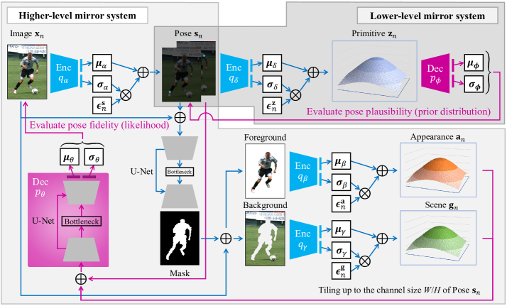Figure 1: An overview of MirrorNet, which consists of generative models of poses and images from latent features and recognition models of poses and latent features from images. The latent features consist of primitives (pose features), appearances (foreground image features), and scenes (background image features). A higher-level image-to-pose-to-image mirror system is integrated with a lower-level pose-to-feature-to-pose mirror system in a hierarchical Bayesian manner, which enables the unsupervised learning of images without pose annotations

1 Introduction

Human beings understand the essence of things by abstraction and embodiment. As Richard P. Feynman, the famous physicist, stated, “What I cannot create, I do not understand” hawking2001universe , abstraction and embodiment are two sides of the same coin. Our hypothesis is that such a bidirectional framework plays a key role in the brain process of recognizing human poses from 2D images, inspired by the mirror neuron system or motor theory known in the field of cognitive neuroscience iacobani2007mirror . In this paper, we focus on the estimation of the 2D pose (joint coordinates) of a person in an image, inspired by the human mirror system.

The standard approach to 2D pose estimation is to train a deep neural network (DNN) that maps an image to a pose in a supervised manner by using a collection of images with pose annotations toshev2014deeppose ; tompson2014joint ; newell2016stacked ; wei2016convolutional ; belagiannis2017recurrent ; yang2017learning ; sun2019deep . Toshev and Szegedy toshev2014deeppose pioneered a method called DeepPose that uses a DNN consisting of convolutional and fully connected layers for the nonlinear regression of 2D joint coordinates from images. Instead of directly using 2D joint coordinates as target data, Thompson et al. tompson2014joint proposed a heatmap representation that indicates the posterior distribution of each joint over pixels. This representation has commonly been used in many state-of-the-art methods of 2D pose estimation newell2016stacked ; wei2016convolutional ; belagiannis2017recurrent ; yang2017learning ; sun2019deep . Note that all these methods focus only on the recognition part of the human mirror system.

Such a supervised approach based on image-to-pose mapping has two major drawbacks. First, the anatomical plausibility of estimated poses is not taken into account. To mitigate this problem, the positional relationships between adjacent joints have often been considered lifshitz2016human ; bulat2016human ; chu2017multi ; tang2018deeply ; nie2018human , and error correction networks carreira2016human ; chen2018cascaded and adversarial networks chen2017adversarial ; chou2018self have been used in a heuristic manner. Second, the performance of the supervised approach is limited by the amount of paired pose-image data. To overcome this limitation, data augmentation techniques peng2018jointly and additional metadata ukita2018semi have been utilized. A unified solution to these complementary problems, however, remains an open question.

In this paper, we propose a hierarchical variational autoencoder (VAE) called MirrorNet that consists of higher- and lower-level mirror systems (Fig. 1). Specifically, we formulate a probabilistic latent variable model that integrates a deep generative model of poses from pose features (called primitives) with that of images from poses and foreground and background features (called appearances and scenes). To estimate poses, pose features, and image features from given images in the framework of amortized variational inference (AVI) kingma2014autoencoding , we introduce a deep recognition model of pose features from poses, that of foreground and background image features from poses and images, and that of poses from images. These generative and recognition models can be trained jointly even from non-annotated images.

A key feature of our semi-supervised method is to consider the anatomical fidelity and plausibility of poses in the estimation process. To make use of both annotated and non-annotated images, our method constructs an image-to-pose-to-image reflective model (i.e., a higher-level mirror system for image understanding) by connecting the image-to-pose recognition model with the pose-to-image generative model. Even when only images without pose annotations are given, the generative model can be used for evaluating the anatomical fidelity of poses estimated by the recognition model (i.e., how consistent the estimated poses are with the given images). In the same way, our method builds a pose-to-feature-to-pose reflective model (i.e., a lower-level mirror system for pose understanding) by connecting the pose-to-feature recognition model with feature-to-pose generative model. This pose VAE can be trained in advance by using a large number of pose data (e.g., those obtained by rendering human 3D models) and then used for evaluating the anatomical plausibility of the estimated poses. Note that the pose VAE cannot be used alone as an evaluator of an estimated pose for a non-annotated image because any plausible pose is allowed even if it does not reflect the image. This is why conventional plausibility-aware methods still need paired data chen2017adversarial ; chen2018cascaded ; chou2018self . The higher- and lower- mirror systems are integrated into MirrorNet and can be trained jointly in a statistically principled manner. In practice, each component of MirrorNet is trained separately by using paired data and then the entire MirrorNet is jointly trained in a semi-supervised manner using both paired and unpaired data for further optimization.

The main contributions of this paper are as follows. We formulate a unified probabilistic model of poses and images, and propose a hierarchical autoencoding variational inference method based on a two-level mirror system for plausibility- and fidelity-aware pose estimation. Our pose estimation method is the first that can use images with and without annotations for semi-supervised learning. We experimentally show that the performance of the image-to-pose recognition model can be improved by integrating the pose-to-image generative model and the pose VAE.

The rest of this paper is organized as follows. Section 2 reviews related work on plausibility-aware pose estimation and fidelity-aware image processing. Section 3 explains the proposed method for unsupervised, supervised, and semi-supervised pose estimation. Section 4 describes the detailed implementation of the proposed method. Section 5 reports comparative experiments conducted for evaluating the proposed method. Section 6 summarizes this paper.

2 Related Work

2D human pose estimation refers to estimating the coordinates of joints of a person in an image, in contrast to skeleton extraction aubert2014poisson ; whytock2014dynamic ; shen2017deepskeleton . This task is challenging because a wide variety of human appearances and background scenes can exist and some joints are often occluded.

For robust pose estimation, Ramanan ramanan2007learning proposed an edge-based model, and Andriluka et al. andriluka2009pictorial introduced a pictorial structure model of human joints. Modeling the human body using tree or graph structures has been intensively studied gkioxari2013articulated ; sapp2010adaptive ; yang2011articulated ; johnson2011learning ; sapp2013modec ; pishchulin2013poselet ; dantone2013human . To improve the accuracy of estimation, one needs to carefully design sophisticated models and features that can appropriately represent the relations between joints.

Toshev and Szegedy toshev2014deeppose proposed a neural pose estimator called DeepPose that estimates the positions of joints by using a DNN consisting of convolutional layers and fully connected layers. DeepPose is the first method that applies deep learning to pose estimation, resulting in significant performance improvement. Instead of directly regressing the coordinates of joints from an image as in DeepPose, Thompson et al. tompson2014joint used a heatmap (pixel-wise likelihood) for representing the distributions of each joint, which has recently become standard. The state-of-the-art methods of 2D pose estimation have been examined from several points of view. For example, intermediate supervision and multi-stage learning were proposed for using the large receptive field of deep convolutional neural networks (CNNs) newell2016stacked ; wei2016convolutional ; belagiannis2017recurrent ; yang2017learning ; sun2019deep . An optimal objective function was proposed for evaluating the relations between pairs of joints lifshitz2016human ; bulat2016human ; chu2017multi ; tang2018deeply . Recently, some studies have assessed the correctness of inferred poses using additional networks chen2018cascaded ; fieraru2018learning ; moon2019posefix or compensated for the lack of data samples with data augmentation ukita2018semi ; peng2018jointly . We here review plausibility-aware methods of pose estimation and fidelity-aware methods of image processing.

2.1 Plausibility-Aware Pose Estimation

A standard way of improving the anatomical plausibility of estimated poses is to focus on the local relations of adjacent joints in pose estimation lifshitz2016human ; bulat2016human ; chu2017multi ; tang2018deeply ; nie2018human or to refine the estimated poses as post-processing. Carreira et al. carreira2016human proposed a self-correcting model based on iterative error feedback. Chen et al. chen2018cascaded , Fieraru et al. fieraru2018learning , and Moon et al. moon2019posefix proposed cascaded networks that recursively refine the estimated poses while referring to the original images. Adversarial networks have often been used to judge whether the estimated poses are anatomically plausible chen2017adversarial ; chou2018self . In addition, Ke et al. ke2018multi proposed a scale-robust method based on a multi-scale network with a body structure-aware loss function. Nie et al. nie2019single proposed a structured pose representation using the displacement in the position of every joint from a root joint position. While these methods can use only paired data for supervised learning, our VAE-based method enables unsupervised learning. In contract to the existing autoencoding approach that aims to extract latent features of poses walker2017pose ; ma2018disentangled , our VAE is used for measuring the plausibility of poses.

To compensate for lack of training data, Ukita and Uematsu ukita2018semi took a weakly supervised approach that uses action labels of images (e.g., baseball and volleyball) to estimate the poses of humans from a part of paired data. Peng et al. peng2018jointly proposed an efficient data augmentation method that generates hard-to-recognize images with adversarial training. Yeh et al. yehchirality used the chirality transform, a geometric transform that generates an antipode of a target, for pose regression. In this paper, we take a different approach based on mirror systems for unsupervised learning such that non-annotated images can be used to improve the performance.

2.2 Fidelity-Aware Image Processing

Mirror structures have been used successfully for various image processing tasks including domain conversion. Kingma and Welling kingma2014autoencoding proposed the VAE that jointly learns a generative model (decoder) of observed variables from latent variables following a prior distribution, and a recognition model (encoder) of the latent variables from the observed variables. It can generate new samples by randomly drawing latent variables from the prior distribution. CycleGAN zhu2017unpaired , DiscoGAN kim2017learning , and DualGAN yi2017dualgan are popular variants of GANs using mirror structures for image-to-image conversion. The key feature of these methods is to consider mutual mappings between domains from unpaired data. Qiao et al. qiao2019mirrorgan recently proposed MirrorGAN for bidirectional inter-domain (text-image) conversion. Yildiri et al. Yildirimeaax5979 proposed an analysis-by-synthesis approach to joint 3D face generation and recognition from a cognitive point of view. The success of these methods indicates the potential of mirror structures for stably training a DNN with unsupervised data. In this paper, we propose the first mirror-structured DNN for human pose estimation that integrates two-level mirror systems in a hierarchically autoencoding variational manner.

3 Proposed Method

Figure 2: The proposed architecture of MirrorNet integrating a VAE for poses (lower-level mirror system) with a pose-conditioned VAE for images (higher-level mirror system) in a hierarchical Bayesian manner. In terms of generative modeling, the decoder of the pose VAE serves as a prior distribution of poses $p(\mathbf{S})$ to evaluate the pose plausibility and the decoder of the image VAE as a likelihood function of poses $p(\mathbf{X}|\mathbf{S})$ to evaluate the pose fidelity. In terms of posterior inference, the encoder of the pose VAE is used as a variational posterior distribution of poses $q(\mathbf{S}|\mathbf{X})$. Such a statistical approach based on a complete probabilistic generative model enables semi-supervised pose estimation using any images with/without pose annotations

This section describes the proposed method based on a fully probabilistic model of poses and images for 2D pose estimation in images of people (Fig. 2). MirrorNet is a hierarchical VAE, one of the techniques of amortized variational inference (AVI) kingma2014autoencoding ; dai2016variational ; mnih2014neural ; rezende2014stochastic , and consists of a VAE of images (i.e., a pose-to-image generative model and an image-to-pose recognition model), and a VAE of poses (i.e., a primitive-to-pose generative model and a pose-to-primitive recognition model). In theory, this model can be trained in an unsupervised manner by using non-annotated images only, or by using unpaired images and poses. In practice, the model is trained in a semi-supervised manner by using partially annotated images. Each model is first trained separately to stabilize the training, and then all models are jointly trained for further optimization. Once the training is completed, only the image-to-pose recognition model is used for pose estimation. The hierarchical autoencoding architecture is effective for estimating poses that are anatomically plausible and have high fidelity to the original images.

3.1 Problem Specification

Let $\mathbf{X}=\{\mathbf{x}_{n}\in\mathbb{R}^{D^{\mathbf{x}}}\}_{n=1}^{N}$ and $\mathbf{S}=\{\mathbf{s}_{n}\in\mathbb{R}^{D^{\mathbf{s}}}\}_{n=1}^{N}$ be a set of images and a set of poses corresponding to $\mathbf{X}$, respectively, where $D^{\mathbf{x}}(\sim\mathcal{O}(10^{6}))$ is the number of dimensions of each image, $D^{\mathbf{s}}(\sim\mathcal{O}(10^{5}))$ is the number of dimensions of each pose, and $N$ is the number of images. We assume that each $\mathbf{x}_{n}$ is an RGB image featuring a single or multiple people, showing all or parts of their bodies, and each $\mathbf{s}_{n}$ is a set of grayscale images, each of which represents the position of a joint using a heatmap tompson2014joint .

Let $\mathbf{A}=\{\mathbf{a}_{n}\in\mathbb{R}^{D^{\mathbf{a}}}\}_{n=1}^{N}$ and $\mathbf{G}=\{\mathbf{g}_{n}\in\mathbb{R}^{D^{\mathbf{g}}}\}_{n=1}^{N}$ be a set of appearances representing the foreground features of $\mathbf{X}$ (e.g., skin and hair colors and textures) and a set of scenes representing the background features of $\mathbf{X}$ (e.g., places, color, and brightness), respectively, where $D^{\mathbf{a}}$ and $D^{\mathbf{g}}$ are the number of dimensions of the latent spaces. These latent features are used in combination with $\mathbf{S}$ for representing $\mathbf{X}$. Let $\mathbf{Z}=\{\mathbf{z}_{n}\in\mathbb{R}^{D^{\mathbf{z}}}\}_{n=1}^{N}$ be a set of primitives representing the features of $\mathbf{S}$ (e.g., scales, positions, and orientations of joints), where $D^{\mathbf{z}}$ is the number of dimensions of the latent space.

Our goal is to train a pose estimator that maps $\mathbf{X}$ to $\mathbf{S}$. Let $M$ be the number of annotated images. In a supervised condition, $\mathbf{X}$ and $\mathbf{S}$ are given as observed data ($M=N$). In an unsupervised condition, only $\mathbf{X}$ is given ($M=0$). In a semi-supervised condition, $\mathbf{X}$ and a part of $\mathbf{S}$, i.e., $\{\mathbf{s}_{n}\}_{n=1}^{M}$, are given.

Figure 3: Three types of statistical inference. The solid and dashed arrows indicate the generative and inference models, respectively, and the shaded circles represent the given data. In the unsupervised learning (Section 3.3), the networks are trained using only images $\mathbf{X}$. In the supervised learning (Section 3.4), the networks are trained using paired data of images $\mathbf{X}$ with poses $\mathbf{S}$. The semi-supervised learning is a mixture of these two conditions

3.2 Generative Modeling

We formulate a unified hierarchical generative model of images $\mathbf{X}$, poses $\mathbf{S}$, appearances $\mathbf{A}$, scenes $\mathbf{G}$, and primitives $\mathbf{Z}$ that integrates a deep generative model of $\mathbf{X}$ from $\mathbf{S}$, $\mathbf{A}$, and $\mathbf{G}$ with a deep generative model of $\mathbf{S}$ from $\mathbf{Z}$ as follows (Fig. 3):

$$\!p(\mathbf{X},\mathbf{S},\mathbf{A},\mathbf{G},\mathbf{Z})$$

$$\!=p_{\theta}(\mathbf{X}|\mathbf{S},\mathbf{A},\mathbf{G})p_{\phi}(\mathbf{S}|\mathbf{Z})p(\mathbf{A})p(\mathbf{G})p(\mathbf{Z})$$

$$\!=\prod_{n=1}^{N}p_{\theta}(\mathbf{x}_{n}|\mathbf{s}_{n},\mathbf{a}_{n},\mathbf{g}_{n})p_{\phi}(\mathbf{s}_{n}|\mathbf{z}_{n})p(\mathbf{a}_{n})p(\mathbf{g}_{n})p(\mathbf{z}_{n}),\!$$ (1)

where $\theta$ and $\phi$ are the sets of trainable parameters of the deep generative models of $\mathbf{x}_{n}$ and $\mathbf{s}_{n}$, respectively. The pose likelihood $p_{\theta}(\mathbf{x}_{n}|\mathbf{s}_{n},\mathbf{a}_{n},\mathbf{g}_{n})$ evaluates the pose fidelity to the given images and the pose prior $p_{\phi}(\mathbf{s}_{n}|\mathbf{z}_{n})$ prevents anatomically implausible pose estimates. The remaining terms are priors of $\mathbf{a}_{n},\mathbf{g}_{n}$, and $\mathbf{z}_{n}$.

The pose-to-image generation model $p_{\theta}(\mathbf{x}_{n}|\mathbf{s}_{n},\mathbf{a}_{n},\mathbf{g}_{n})$ and the primitive-to-pose generation model $p_{\phi}(\mathbf{s}_{n}|\mathbf{z}_{n})$ are both formulated as follows:

$$p_{\theta}(\mathbf{x}_{n}|\mathbf{s}_{n},\mathbf{a}_{n},\mathbf{g}_{n})$$

$$=\mathcal{N}(\mathbf{x}_{n};\mu_{\theta}(\mathbf{s}_{n},\mathbf{a}_{n},\mathbf{g}_{n}),\sigma_{\theta}^{2}(\mathbf{s}_{n},\mathbf{a}_{n},\mathbf{g}_{n})\mathbf{I}_{D^{\mathbf{x}}}),$$ (2)

$$p_{\phi}(\mathbf{s}_{n}|\mathbf{z}_{n})=\mathcal{N}(\mathbf{s}_{n};\mu_{\phi}(\mathbf{z}_{n}),\sigma_{\phi}^{2}(\mathbf{z}_{n})\mathbf{I}_{D^{\mathbf{s}}}),$$ (3)

where $\mathbf{\mu}_{\theta}(\mathbf{s}_{n},\mathbf{a}_{n},\mathbf{g}_{n})$ and $\sigma_{\theta}(\mathbf{s}_{n},\mathbf{a}_{n},\mathbf{g}_{n})$ are the outputs of a DNN with parameter $\theta$ that takes $\mathbf{s}_{n},\mathbf{a}_{n}$, and $\mathbf{g}_{n}$ as input, and $\mathbf{\mu}_{\phi}(\mathbf{z}_{n})$ and $\sigma_{\phi}(\mathbf{z}_{n})$ are the outputs of a DNN with parameters $\phi$ that takes $\mathbf{z}_{n}$ as input. The priors $p(\mathbf{a}_{n})$, $p(\mathbf{g}_{n})$, and $p(\mathbf{z}_{n})$ are set to the standard Gaussian distributions as follows:

$$p(\mathbf{a}_{n}) =\mathcal{N}(\mathbf{a}_{n};\mathbf{0}_{D^{\mathbf{a}}},\mathbf{I}_{D^{\mathbf{a}}}),$$ (4)

$$p(\mathbf{g}_{n}) =\mathcal{N}(\mathbf{g}_{n};\mathbf{0}_{D^{\mathbf{g}}},\mathbf{I}_{D^{\mathbf{g}}}),$$ (5)

$$p(\mathbf{z}_{n}) =\mathcal{N}(\mathbf{z}_{n};\mathbf{0}_{D^{\mathbf{z}}},\mathbf{I}_{D^{\mathbf{z}}}),$$ (6)

where $\mathbf{0}_{D^{\dagger}}$ $(D^{\dagger}=\{D^{\mathbf{a}},D^{\mathbf{g}},D^{\mathbf{z}}\})$ and $\mathbf{I}_{D^{\dagger}}$ are the zero vector of size $D^{\dagger}$ and the identity matrix of size $D^{\dagger}$, respectively.

3.3 Unsupervised Learning

We explain the unsupervised learning of the proposed model using only images $\mathbf{X}$, which is the basis for practical semi-supervised learning using partially annotated images (Section 3.4). Given a set of images $\mathbf{X}$ as observed data, our goal is to infer the distribution of the latent variables $\mathbf{\Omega}\equiv(\mathbf{S},\mathbf{A},\mathbf{G},\mathbf{Z})$. We estimate optimal parameters $\theta^{*}$ and $\phi^{*}$ in the framework of maximum likelihood estimation as follows:

$$\theta^{*},\phi^{*}=\mathop{\rm argmax}_{\theta,\phi}p(\mathbf{X}),$$ (7)

and $p(\mathbf{X})$ is the marginal likelihood given by

$$p(\mathbf{X})=\int\!p(\mathbf{X},\mathbf{\Omega})d\mathbf{\Omega}.$$ (8)

where $p(\mathbf{X},\mathbf{\Omega})$ is the joint probability distribution given by Eq. (1).

Because Eq. (8) is analytically intractable, we use an amortized variational inference (AVI) technique kingma2014autoencoding ; dai2016variational ; mnih2014neural ; rezende2014stochastic that introduces an arbitrary variational posterior distribution $q(\mathbf{\Omega}|\mathbf{X})$ and makes it as close to the true posterior distribution $p(\mathbf{\Omega}|\mathbf{X})$ (Section 3.3.1). The minimization of the Kullback–Leibler (KL) divergence between these posteriors is equivalent to the maximization of a variational lower bound $\mathcal{L}$ of $\log p(\mathbf{X})$ with respect to $q(\mathbf{\Omega}|\mathbf{X})$. Thus, the optimal parameters $\theta^{*}$ and $\phi^{*}$ can be obtained by maximizing the variational lower bound $\mathcal{L}$ instead of $\log p(\mathbf{X})$ (Section 3.3.2).

3.3.1 Variational Lower Bound

Using Jensen’s inequality, a variational lower bound $\mathcal{L}^{\mathbf{X}}$ of $\log p(\mathbf{X})$ can be derived as follows:

$$\log p(\mathbf{X}) =\log\int\!p(\mathbf{X},\mathbf{\Omega})d\mathbf{\Omega}$$

$$=\log\int\!\frac{q(\mathbf{\Omega}|\mathbf{X})}{q(\mathbf{\Omega}|\mathbf{X})}p(\mathbf{X},\mathbf{\Omega})d\mathbf{\Omega}$$

$$\geq\int\!q(\mathbf{\Omega}|\mathbf{X})\log\frac{p(\mathbf{X},\mathbf{\Omega})}{q(\mathbf{\Omega}|\mathbf{X})}d\mathbf{\Omega}\overset{\mbox{\tiny def}}{=}\mathcal{L}^{\mathbf{X}},$$ (9)

where the equality holds, i.e., $\mathcal{L}^{\mathbf{X}}$ is maximized, if and only if $q(\mathbf{\Omega}|\mathbf{X})=p(\mathbf{\Omega}|\mathbf{X})$. Because this equality condition cannot be computed analytically, $q(\mathbf{\Omega}|\mathbf{X})$ is approximated by a factorized form as follows:

$$q(\mathbf{\Omega}|\mathbf{X})=q_{\alpha}(\mathbf{S}|\mathbf{X})q_{\beta}(\mathbf{A}|\mathbf{S},\mathbf{X})q_{\gamma}(\mathbf{G}|\mathbf{S},\mathbf{X})q_{\delta}(\mathbf{Z}|\mathbf{S})$$

$$\!=\prod_{n=1}^{N}q_{\alpha}(\mathbf{s}_{n}|\mathbf{x}_{n})q_{\beta}(\mathbf{a}_{n}|\mathbf{s}_{n},\mathbf{x}_{n})q_{\gamma}(\mathbf{g}_{n}|\mathbf{s}_{n},\mathbf{x}_{n})q_{\delta}(\mathbf{z}_{n}|\mathbf{s}_{n}),$$ (10)

where $\alpha$, $\beta$, $\gamma$, and $\delta$ are the sets of parameters of these four variational distributions, respectively.

In the statistical framework of AVI, we introduce a DNN-based posterior distribution $q(\mathbf{\Omega}|\mathbf{X})$ such that the complex true posterior distribution $p(\mathbf{\Omega}|\mathbf{X})$ can be well approximated by $q(\mathbf{\Omega}|\mathbf{X})$. Specifically, we introduce a deep image-to-pose model $q_{\alpha}(\mathbf{s}_{n}|\mathbf{x}_{n})$, a deep image-to-appearance model $q_{\beta}(\mathbf{a}_{n}|\mathbf{s}_{n},\mathbf{x}_{n})$, a deep image-to-scene model $q_{\gamma}(\mathbf{g}_{n}|\mathbf{s}_{n},\mathbf{x}_{n})$, and a deep pose-to-primitive model $q_{\delta}(\mathbf{z}_{n}|\mathbf{s}_{n})$ as follows:

$$q_{\alpha}(\mathbf{s}_{n}|\mathbf{x}_{n}) =\mathcal{N}(\mathbf{s}_{n};\mathbf{\mu}_{\alpha}(\mathbf{x}_{n}),\sigma_{\alpha}^{2}(\mathbf{x}_{n})\mathbf{I}_{D^{\mathbf{s}}}),$$ (11)

$$q_{\beta}(\mathbf{a}_{n}|\mathbf{s}_{n},\mathbf{x}_{n}) =\mathcal{N}(\mathbf{a}_{n};\mathbf{\mu}_{\beta}(\mathbf{s}_{n},\mathbf{x}_{n}),\mathbf{\sigma}_{\beta}^{2}(\mathbf{s}_{n},\mathbf{x}_{n})\mathbf{I}_{D^{\mathbf{a}}}),\!$$ (12)

$$q_{\gamma}(\mathbf{g}_{n}|\mathbf{s}_{n},\mathbf{x}_{n}) =\mathcal{N}(\mathbf{g}_{n};\mathbf{\mu}_{\gamma}(\mathbf{s}_{n},\mathbf{x}_{n}),\mathbf{\sigma}_{\gamma}^{2}(\mathbf{s}_{n},\mathbf{x}_{n})\mathbf{I}_{D^{\mathbf{g}}}),\!$$ (13)

$$q_{\delta}(\mathbf{z}_{n}|\mathbf{s}_{n}) =\mathcal{N}(\mathbf{z}_{n};\mathbf{\mu}_{\delta}(\mathbf{s}_{n}),\mathbf{\sigma}_{\delta}^{2}(\mathbf{s}_{n})\mathbf{I}_{D^{\mathbf{z}}}),$$ (14)

where $\mathbf{\mu}_{\alpha}(\mathbf{x}_{n})$ and $\sigma_{\alpha}(\mathbf{x}_{n})$ are the outputs of a DNN with parameters $\alpha$ that takes $\mathbf{x}_{n}$ as input, $\mathbf{\mu}_{{\ddagger}}(\mathbf{s}_{n},\mathbf{x}_{n})$ and $\mathbf{\sigma}_{{\ddagger}}(\mathbf{s}_{n},\mathbf{x}_{n})$ $({\ddagger}=\beta\ \mathrm{or}\ \gamma)$ are the outputs of a DNN with parameters ${\ddagger}$ that takes $\mathbf{s}_{n}$ and $\mathbf{x}_{n}$ as input, and $\mathbf{\mu}_{\delta}(\mathbf{s}_{n})$ and $\mathbf{\sigma}_{\delta}(\mathbf{s}_{n})$ are the outputs of a DNN with parameters $\delta$ that takes $\mathbf{s}_{n}$ as input.

Substituting both of the generative model given by Eq. (1) with Eqs. (2)–(6) and the recognition model given by Eq. (10) with Eqs. (11)–(14) into Eq. (9), the variational lower bound $\mathcal{L}^{\mathbf{X}}$ can be rewritten as the sum of $\{\mathcal{L}^{\mathbf{X}}_{n}\}_{n=1}^{N}$ ($\mathcal{L}^{\mathbf{X}}=\sum_{n}\mathcal{L}^{\mathbf{X}}_{n}$) as follows (Appendix A):

$$\mathcal{L}^{\mathbf{X}}_{n}= \ \mathbb{E}_{q}[\log p_{\theta}(\mathbf{x}_{n}|\mathbf{s}_{n},\mathbf{a}_{n},\mathbf{g}_{n})+\log p_{\phi}(\mathbf{s}_{n}|\mathbf{z}_{n})$$

$$+\log p(\mathbf{a}_{n})+\log p(\mathbf{g}_{n})+\log p(\mathbf{z}_{n})$$

$$-\log q_{\alpha}(\mathbf{s}_{n}|\mathbf{x}_{n})-\log q_{\beta}(\mathbf{a}_{n}|\mathbf{s}_{n},\mathbf{x}_{n})$$

$$-\log q_{\gamma}(\mathbf{g}_{n}|\mathbf{s}_{n},\mathbf{x}_{n})-\log q_{\delta}(\mathbf{z}_{n}|\mathbf{s}_{n})]$$

$$= \ \mathbb{E}_{q}[\log p_{\theta}(\mathbf{x}_{n}|\mathbf{s}_{n},\mathbf{a}_{n},\mathbf{g}_{n})]$$

$$+\mathbb{E}_{q}[\log p_{\phi}(\mathbf{s}_{n}|\mathbf{z}_{n})]$$

$$-\mathbb{E}_{q}[\log q_{\alpha}(\mathbf{s}_{n}|\mathbf{x}_{n})]$$

$$-\mathbb{E}_{q}[\mbox{KL}(q_{\beta}(\mathbf{a}_{n}|\mathbf{s}_{n},\mathbf{x}_{n})||p(\mathbf{a}_{n}))]$$

$$-\mathbb{E}_{q}[\mbox{KL}(q_{\gamma}(\mathbf{g}_{n}|\mathbf{s}_{n},\mathbf{x}_{n})||p(\mathbf{g}_{n}))]$$

$$-\mathbb{E}_{q}[\mbox{KL}(q_{\delta}(\mathbf{z}_{n}|\mathbf{s}_{n})||p(\mathbf{z}_{n}))],$$ (15)

where the first term represents the fidelity of a pose $\mathbf{s}_{n}$ with an original image $\mathbf{x}_{n}$ having features $\mathbf{a}_{n}$ and $\mathbf{g}_{n}$, the second term represents the plausibility of $\mathbf{s}_{n}$, the third term prevents the overfitting of the recognition model $\alpha$, and the fourth to sixth terms evaluate the similarities between the recognition models $\beta$, $\gamma$, and $\delta$ and the priors on $\mathbf{a}_{n}$, $\mathbf{g}_{n}$, and $\mathbf{z}_{n}$, respectively.

3.3.2 Parameter Optimization

Because Eq. (15) still includes intractable expectations, we perform Monte Carlo integration using samples $\mathbf{s}_{n}$, $\mathbf{a}_{n}$, $\mathbf{g}_{n}$, and $\mathbf{z}_{n}$ obtained by reparametrization trick kingma2014autoencoding as follows:

$$\mathbf{\epsilon}^{\mathbf{s}}_{n} \sim\mathcal{N}(\mathbf{0},\mathbf{I}_{D^{\mathbf{s}}}),$$ (16)

$$\mathbf{\epsilon}^{\mathbf{a}}_{n} \sim\mathcal{N}(\mathbf{0},\mathbf{I}_{D^{\mathbf{a}}}),$$ (17)

$$\mathbf{\epsilon}^{\mathbf{g}}_{n} \sim\mathcal{N}(\mathbf{0},\mathbf{I}_{D^{\mathbf{g}}}),$$ (18)

$$\mathbf{\epsilon}^{\mathbf{z}}_{n} \sim\mathcal{N}(\mathbf{0},\mathbf{I}_{D^{\mathbf{z}}}),$$ (19)

$$\mathbf{s}_{n} =\mathbf{\mu}_{\alpha}(\mathbf{x}_{n})+\mathbf{\epsilon}^{\mathbf{s}}_{n}\odot\mathbf{\sigma}_{\alpha}(\mathbf{x}_{n}),$$ (20)

$$\mathbf{a}_{n} =\mathbf{\mu}_{\beta}(\mathbf{s}_{n},\mathbf{x}_{n})+\mathbf{\epsilon}^{\mathbf{a}}_{n}\odot\mathbf{\sigma}_{\beta}(\mathbf{s}_{n},\mathbf{x}_{n}),$$ (21)

$$\mathbf{g}_{n} =\mathbf{\mu}_{\gamma}(\mathbf{s}_{n},\mathbf{x}_{n})+\mathbf{\epsilon}^{\mathbf{g}}_{n}\odot\mathbf{\sigma}_{\gamma}(\mathbf{s}_{n},\mathbf{x}_{n}),$$ (22)

$$\mathbf{z}_{n} =\mathbf{\mu}_{\delta}(\mathbf{s}_{n})+\mathbf{\epsilon}^{\mathbf{z}}_{n}\odot\mathbf{\sigma}_{\delta}(\mathbf{s}_{n}),$$ (23)

where $\odot$ indicates the element-wise product. Although in theory a sufficient number of samples should be generated to perform accurate Monte Carlo integration, we generate only one sample for each variable as in the standard VAE kingma2014autoencoding .

Using these tricks, the lower bound $\mathcal{L}^{\mathbf{X}}$ given by Eq. (15) can be approximately computed, and can thus be maximized with respect to $\theta$, $\phi$, $\alpha$, $\beta$, $\gamma$, and $\delta$ (Fig. 2). First, the recognition models $\alpha$, $\beta$, $\gamma$, and $\delta$ are used to deterministically generate samples $\mathbf{s}_{n}$, $\mathbf{a}_{n}$, $\mathbf{g}_{n}$, and $\mathbf{z}_{n}$ in Eqs. (20)–(23), and to calculate the last four regularization terms of Eq. (15), respectively. Given the samples $\mathbf{s}_{n}$, $\mathbf{a}_{n}$, $\mathbf{g}_{n}$, and $\mathbf{z}_{n}$, the generative models $\theta$ and $\phi$ are used to calculate the first two reconstruction terms of Eq. (15), respectively. The recognition models $\alpha$, $\beta$, $\gamma$, and $\delta$, and the generative models $\phi$ and $\theta$ can thus be concatenated in this order with the reparametrization trick given by Eqs. (20)–(23), and are jointly optimized in an autoencoding manner with an objective function given by Eq. (15).

3.4 Supervised Learning

We explain the supervised learning of the proposed model using paired data of $\mathbf{X}$ and $\mathbf{S}$. This approach follows the manner of the semi-supervised learning of a VAE kingma2014semisupervised . While the variational lower bound $\mathcal{L}^{\mathbf{X}}$ of $\log p(\mathbf{X})$ is maximized in the unsupervised condition (Section 3.3), we aim to maximize the variational lower bound $\mathcal{L}^{\mathbf{X},\mathbf{S}}$ of $\log p(\mathbf{X},\mathbf{S})$, which is given by

$$\log p(\mathbf{X},\mathbf{S}) =\log\!\int\!p(\mathbf{X},\mathbf{\Omega})d\mathbf{\Theta}$$

$$=\log\!\int\!\frac{q(\mathbf{\Theta}|\mathbf{S},\mathbf{X})}{q(\mathbf{\Theta}|\mathbf{S},\mathbf{X})}p(\mathbf{X},\mathbf{\Omega})d\mathbf{\Theta}$$

$$\geq\int\!q(\mathbf{\Theta}|\mathbf{S},\mathbf{X})\log\frac{p(\mathbf{X},\mathbf{\Omega})}{q(\mathbf{\Theta}|\mathbf{S},\mathbf{X})}d\mathbf{\Theta}$$

$$\overset{\mbox{\tiny def}}{=}\mathcal{L}^{\mathbf{X},\mathbf{S}},$$ (24)

where $\mathbf{\Theta}=\mathbf{\Omega}\!\setminus\!\mathbf{S}=\{\mathbf{A},\mathbf{G},\mathbf{Z}\}$. As in Eq. (10), $q(\mathbf{\Theta}|\mathbf{S},\mathbf{X})$ is factorized as

$$q(\mathbf{\Theta}|\mathbf{S},\mathbf{X})$$

$$=q_{\beta}(\mathbf{A}|\mathbf{S},\mathbf{X})q_{\gamma}(\mathbf{G}|\mathbf{S},\mathbf{X})q_{\delta}(\mathbf{Z}|\mathbf{S})$$

$$=\prod_{n=1}^{N}q_{\beta}(\mathbf{a}_{n}|\mathbf{s}_{n},\mathbf{x}_{n})q_{\gamma}(\mathbf{g}_{n}|\mathbf{s}_{n},\mathbf{x}_{n})q_{\delta}(\mathbf{z}_{n}|\mathbf{s}_{n}),$$ (25)

where $q_{\beta}(\mathbf{a}_{n}|\mathbf{s}_{n},\mathbf{x}_{n})$, $q_{\gamma}(\mathbf{g}_{n}|\mathbf{s}_{n},\mathbf{x}_{n})$, and $q_{\delta}(\mathbf{z}_{n}|\mathbf{s}_{n})$ are given by Eqs. (12)–(14), respectively. Substituting both of the probabilistic model given by Eq. (1) with Eqs. (2)–(6) and the inference model given by Eq. (25) with Eqs. (12)–(14) into Eq. (24), $\mathcal{L}^{\mathbf{X},\mathbf{S}}$ can be rewritten as the sum of $\{\mathcal{L}^{\mathbf{X},\mathbf{S}}_{n}\}_{n=1}^{N}$ ($\mathcal{L}^{\mathbf{X},\mathbf{S}}=\sum_{n}\mathcal{L}^{\mathbf{X},\mathbf{S}}_{n}$) as follows (Appendix A):

$$\mathcal{L}^{\mathbf{X},\mathbf{S}}_{n}= \ \mathbb{E}_{q}[\log p_{\theta}(\mathbf{x}_{n}|\mathbf{s}_{n},\mathbf{a}_{n},\mathbf{g}_{n})+\log p_{\phi}(\mathbf{s}_{n}|\mathbf{z}_{n})$$

$$+\log p(\mathbf{a}_{n})+\log p(\mathbf{g}_{n})+\log p(\mathbf{z}_{n})$$

$$-\log q_{\beta}(\mathbf{a}_{n}|\mathbf{s}_{n},\mathbf{x}_{n})-\log q_{\gamma}(\mathbf{g}_{n}|\mathbf{s}_{n},\mathbf{x}_{n})$$

$$-\log q_{\delta}(\mathbf{z}_{n}|\mathbf{s}_{n})]$$

$$= \ \mathbb{E}_{q}[\log p_{\theta}(\mathbf{x}_{n}|\mathbf{s}_{n},\mathbf{a}_{n},\mathbf{g}_{n})]$$

$$+\mathbb{E}_{q}[\log p_{\phi}(\mathbf{s}_{n}|\mathbf{z}_{n})]$$

$$-\mbox{KL}(q_{\beta}(\mathbf{a}_{n}|\mathbf{s}_{n},\mathbf{x}_{n})||p(\mathbf{a}_{n}))$$

$$-\mbox{KL}(q_{\gamma}(\mathbf{g}_{n}|\mathbf{s}_{n},\mathbf{x}_{n})||p(\mathbf{g}_{n}))$$

$$-\mbox{KL}(q_{\delta}(\mathbf{z}_{n}|\mathbf{s}_{n})||p(\mathbf{z}_{n})).$$ (26)

A major problem in such supervised learning is that the recognition model $q_{\alpha}(\mathbf{s}_{n}|\mathbf{x}_{n})$, which plays a central role for human pose estimation from images, cannot be trained because it does not appear in Eq. (26). To solve this problem, we add a term to assess the predictive performance of $q_{\alpha}(\mathbf{s}_{n}|\mathbf{x}_{n})$ to $\mathcal{L}_{n}$, following kingma2014semisupervised as

$$\mathcal{L}^{\mathbf{X},\mathbf{S}}_{n,\lambda}=\mathcal{L}^{\mathbf{X},\mathbf{S}}_{n}+\lambda\log q_{\alpha}(\mathbf{s}_{n}|\mathbf{x}_{n}),$$ (27)

$$\log q_{\alpha}(\mathbf{s}_{n}|\mathbf{x}_{n})$$

$$=-\frac{1}{2}\sum^{D^{\mathbf{s}}}_{d_{s}=1}\left(\log\left(2\pi\sigma^{2}_{\alpha,d_{s}}(\mathbf{x}_{n})\right)+\frac{(\mathbf{s}_{n}-\mu_{\alpha,d_{s}}(\mathbf{x}_{n}))^{2}}{\sigma_{\alpha,d_{s}}^{2}(\mathbf{x}_{n})}\right),$$ (28)

where $\lambda$ is a hyperparameter that controls the balance between purely generative learning and purely discriminative learning. In our method, we used $\lambda=0.01$ in all experiments. The new objective function $\mathcal{L}^{\mathbf{X},\mathbf{S}}_{\lambda}=\sum_{n}\mathcal{L}^{\mathbf{X},\mathbf{S}}_{n,\lambda}$ can be maximized with respect to $\theta$, $\phi$, $\alpha$, $\beta$, $\gamma$, and $\delta$ jointly in the same way as the unsupervised learning described in Section 3.3.2, where $\mathbf{a}_{n}$, $\mathbf{g}_{n}$, and $\mathbf{z}_{n}$ are obtained by using Eqs. (21)–(23), and $\mathbf{s}_{n}$ is given.

3.5 Semi-supervised Learning

In the semi-supervised condition, where $\mathbf{X}$ is only partially annotated, we define a new objective function $\mathcal{L}$ by accumulating $\mathcal{L}^{\mathbf{X}}_{n}$ used for unsupervised learning or $\mathcal{L}^{\mathbf{X},\mathbf{S}}_{n,\lambda}$ used for supervised learning as follows:

$$\mathcal{L}\overset{\mbox{\tiny def}}{=}\sum_{n:\ \mbox{\scriptsize$\mathbf{x}_{n}$ is given}}\mathcal{L}^{\mathbf{X}}_{n}+\sum_{n:\ \mbox{\scriptsize$\mathbf{x}_{n}$ \& $\mathbf{s}_{n}$ are given}}\mathcal{L}^{\mathbf{X},\mathbf{S}}_{n,\lambda}.$$ (29)

All generation and recognition models can be trained for all samples regardless of the availability of their annotations. In practice, it is effective to pre-train each model in advance.

4 Implementation

This section describes the implementation of MirrorNet, which is based on curriculum learning. First, we separately pre-train the components of MirrorNet, i.e., the pose recognizer $\alpha$ (Section 4.1), the pose-conditioned image VAE with the generator $\theta$ and the recognizers $\beta$ and $\gamma$ (Section 4.2), and the pose VAE with the generator $\phi$ and the recognizer $\delta$ (Section 4.3). We then train the whole MirrorNet under a supervised condition (Section 3.4) and further optimize it under a semi-supervised condition (Section 3.5).

Note that, as shown in Fig. 2, the pose-conditioned image VAE has a human mask estimator as a subcomponent for separating an image into foreground and background images; this helps to stabilize the training of MirrorNet.

4.1 Pose Recognizer

The image-to-pose recognizer $\alpha$ is of most interest in pose estimation, and is pre-trained in a supervised manner by using paired data of $\mathbf{X}$ and $\mathbf{S}$. We maximize an objective function given by

$$\mathcal{L}_{n}(\alpha)\overset{\mbox{\tiny def}}{=}\log q_{\alpha}(\mathbf{s}_{n}|\mathbf{x}_{n}),$$ (30)

where the variance $\sigma_{\alpha}^{2}(\mathbf{x}_{n})$ is fixed to 0.01 for stability.

The network $\alpha$ can be implemented with any DNN that outputs the heatmaps of joint positions. For this part, our implementation has three variations: a stack of eight residual hourglasses newell2016stacked , ResNet-50 (baseline) xiao2018simple , and high-resolution subnetworks sun2019deep .

4.2 Pose-conditioned Image VAE

The pose-conditioned image VAE consisting of the image-to-appearance recognizer $\beta$, the image-to-scene recognizer $\gamma$ (encoders), and the appearance/scene-to-image generator $\theta$ (decoder) is pre-trained in an unsupervised manner by using paired data of $\mathbf{X}$ and $\mathbf{S}$. We maximize a variational lower bound $\mathcal{L}(\theta,\beta,\gamma)$ of the marginal log likelihood $\log p(\mathbf{X}|\mathbf{S})$. More specifically, we have

$$\log p(\mathbf{x}_{n}|\mathbf{s}_{n})$$

$$\geq\ \mathbb{E}_{q}[\log p_{\theta}(\mathbf{x}_{n}|\mathbf{s}_{n},\mathbf{g}_{n})+\log p(\mathbf{a}_{n})+\log p(\mathbf{g}_{n})$$

$$\>\>\>\>\>\>\>\>\>\>\>-\log q_{\beta}(\mathbf{a}_{n}|\mathbf{s}_{n},\mathbf{x}_{n})-\log q_{\gamma}(\mathbf{g}_{n}|\mathbf{s}_{n},\mathbf{x}_{n})]$$

$$=\ \mathbb{E}_{q}[\log p_{\theta}(\mathbf{x}_{n}|\mathbf{s}_{n},\mathbf{a}_{n},\mathbf{g}_{n})]$$

$$\>\>\>\>\>\>\>\>\>\>\>-\mbox{KL}(q_{\beta}(\mathbf{a}_{n}|\mathbf{s}_{n},\mathbf{x}_{n})||p(\mathbf{a}_{n}))$$

$$\>\>\>\>\>\>\>\>\>\>\>-\mbox{KL}(q_{\gamma}(\mathbf{g}_{n}|\mathbf{s}_{n},\mathbf{x}_{n})||p(\mathbf{g}_{n}))$$

$$\overset{\mbox{\tiny def}}{=}\mathcal{L}_{n}(\theta,\beta,\gamma),$$ (31)

where $\mathcal{L}(\theta,\beta,\gamma)=\sum_{n=1}^{N}\mathcal{L}_{n}(\theta,\beta,\gamma)$. The three networks $\theta$, $\beta$, and $\gamma$ can be optimized jointly by using the reparametrization tricks kingma2014autoencoding given by Eq. (21) and Eq. (22), where the variance $\sigma_{\theta}^{2}(\mathbf{s}_{n},\mathbf{a}_{n},\mathbf{g}_{n})$ of the generator $\theta$ is fixed to 1 for stability.

To encourage the disentanglement between the foreground features (appearance) $\mathbf{a}_{n}$ and the background features (scene) $\mathbf{g}_{n}$, we separately input foreground and background parts of the original image $\mathbf{x}_{n}$ into the two encoders $\beta$ and $\gamma$, respectively, instead of directly feeding $\mathbf{x}_{n}$ into $\beta$ and $\gamma$. Specifically, an image $\mathbf{x}^{*}_{n}\in\mathbb{R}^{D^{\mathbf{x}^{*}}}$, a reduced-size version of $\mathbf{x}_{n}$, is first split into foreground and background images $\mathbf{x}^{\mathrm{fg}}_{n}$ and $\mathbf{x}^{\mathrm{bg}}_{n}$ as follows:

$$\mathbf{x}^{\mathrm{fg}}_{n} =\mathbf{x}^{*}_{n}\odot\mathbf{w}_{n},$$ (32)

$$\mathbf{x}^{\mathrm{bg}}_{n} =\mathbf{x}^{*}_{n}\odot(\mathbf{1}-\mathbf{w}_{n}),$$ (33)

where $\odot$ indicates the element-wise product and $\mathbf{w}_{n}\in\mathbb{R}^{D^{\mathbf{x}^{*}}}$ represents a mask image estimated from $\mathbf{x}^{*}_{n}$ with the additional information of the pose $\mathbf{s}_{n}$. In this paper, we use a neural mask estimator $\psi$ trained in a supervised manner such that the mean squared error between the estimated and ground-truth masks is minimized.

Figure 4: The network architecture common in the recognizers $\beta$ and $\gamma$ of the pose-conditioned image VAE taking as input foreground and background images $\mathbf{x}_{n}^{\mathrm{fg}}$ and $\mathbf{x}_{n}^{\mathrm{bg}}$ ($c=3$), respectively, and the recognizer $\delta$ of the pose VAE taking as input the pose $\mathbf{s}_{n}$ ($c$ is the number of joints)

Figure 5: Layers used for implementing DNNs

Figure 6: The network architecture of the generator $\theta$ of pose VAE taking as input the primitives $\mathbf{z}_{n}$ and yielding the mean $\mu_{\phi}(\mathbf{z}_{n})$ and variance $\sigma_{\phi}(\mathbf{z}_{n})$

Figure 7: The network architecture of the generator $\theta$ of the pose-conditioned Image VAE taking as input the pose $\mathbf{s}_{n}$, the appearance $\mathbf{a}_{n}$, and the scene $\mathbf{g}_{n}$ and yielding the mean $\mu_{\theta}(\mathbf{a}_{n},\mathbf{g}_{n},\mathbf{s}_{n})$ and the variance $\sigma_{\theta}(\mathbf{a}_{n},\mathbf{g}_{n},\mathbf{s}_{n})$

The recognizers $\beta$ and $\gamma$ are implemented as stacks of four residual blocks he2016deep (Fig. 4 and Fig. 5). Unlike the original ResNet, a branching architecture is introduced in the last layer to output the mean and variance of the posterior Gaussian distribution. The generator $\theta$ is implemented with a U-Net ronneberger2015u that takes as input a stack of the heatmaps of the joints given by $\mathbf{s}_{n}$ and the latent variables $\mathbf{a}_{n}$ and $\mathbf{g}_{n}$, where a branching architecture is introduced in the last layer to evaluate the pose fidelity with $\mathbf{x}_{n}$ (Fig. 7). The mask estimator $\psi$ is implemented as a U-Net ronneberger2015u that takes as input a shrunk image $\mathbf{x}^{*}_{n}$ and a stack of the heatmaps of the joints given by $\mathbf{s}_{n}$ and outputs a mask image $\mathbf{w}_{n}$. To obtain sharper mask images, we apply a sigmoid function, $\varsigma(x)=(1+\exp{(-10x)})^{-1}$, to every element of the output $\mathbf{w}_{n}$ of the pre-trained estimator $\psi$.

4.3 Pose VAE

The pose VAE consisting of the pose-to-primitive recognizer $\delta$ and the primitive-to-pose generator $\phi$ (decoder) is pre-trained in an unsupervised manner by using only $\mathbf{S}$. We maximize a variational lower bound $\mathcal{L}(\phi,\delta)$ of the marginal log likelihood $\log p(\mathbf{S})$ evaluating the pose plausibility. More specifically, we have

$$\log p(\mathbf{s}_{n})$$

$$\geq\ \mathbb{E}_{q}\!\left[\log p_{\phi}(\mathbf{s}_{n}|\mathbf{z}_{n})+\log p(\mathbf{z}_{n})-\log q_{\delta}(\mathbf{z}_{n}|\mathbf{s}_{n})\right]$$

$$=\ \mathbb{E}_{q}[\log p_{\phi}(\mathbf{s}_{n}|\mathbf{z}_{n})]-\mbox{KL}(q_{\delta}(\mathbf{z}_{n}|\mathbf{s}_{n})||p(\mathbf{z}_{n}))$$

$$\overset{\mbox{\tiny def}}{=}\ \mathcal{L}_{n}(\phi,\delta),$$ (34)

where $\mathcal{L}(\phi,\delta)=\sum_{n=1}^{N}\mathcal{L}_{n}(\phi,\delta)$. The two networks $\phi$ and $\delta$ can be optimized jointly by using the reparametrization trick kingma2014autoencoding given by Eq. (23), where the variance $\sigma_{\phi}^{2}$ of the generator $\phi$ is fixed to 1 for stability.

The recognizer $\delta$ is implemented in the same way as the recognizers $\beta$ and $\gamma$ except that it has a different input dimension (Fig. 4). The generator $\phi$ is implemented as a three-layered transposed convolutional network, where a branching architecture was introduced in the last layer to evaluate the pose plausibility (Fig. 6).

5 Evaluation

This section reports comparative experiments conducted for evaluating the effectiveness of our semi-supervised plausibility- and fidelity-aware pose estimation method. Our goal is to train a neural pose estimator that detects the coordinates of 16 joints (namely, right ankle, right knee, right hip, left hip, left knee, left ankle, pelvis, thorax, upper neck, head top, right wrist, right elbow, right shoulder, left shoulder, left elbow, and left wrist, as shown in Fig. 8) from an image. We here validate two hypotheses: (A) under a supervised condition, the proposed method based on the joint training of the generative and recognition models outperforms conventional methods based on an image-to-pose recognition model, and (B) under a semi-supervised condition, non-annotated images can be used for improving the performance thanks to the power of the mirror architecture.

5.1 Datasets and Criteria

We used two standard datasets that have widely been used in conventional studies on pose estimation.

5.1.1 Leeds Sports Pose (LSP) Dataset

The LSP dataset with its extension johnson2010clustered ; johnson2011learning contains 12K images of sports activities (11K for training and 1K for testing) in total. Each image originally has an annotation about the coordinates of the 14 joints except for the pelvis and thorax. We estimated the coordinate of the pelvis by averaging the coordinates of the left and right hips and the coordinate of the thorax by averaging the coordinates of the left and right shoulders. Each image was cropped to a square region centering on a person and then scaled to $D^{\mathbf{x}}=256\times 256$.

The performance of pose estimation was measured with the percentage of correct keypoints (PCK) yang2013articulated . The estimated coordinate of a joint was judged as correct if it was within $\tau\times\max(h,w)$ pixels around the ground-truth coordinate, where $\tau$ is a normalized distance, and $h$ and $w$ are the height and width of the tightly cropped bounding box of the person, respectively. We used $\tau=0.2$ in our experiment.

Figure 8: sixteen joints considered in our experiments

5.1.2 MPII Human Pose (MPII) Dataset

The MPII dataset andriluka14cvpr contains around 25K images of daily activities (22K for training and 3K for testing). Each image has an annotation about the coordinates of the 16 joints and was cropped to a square region centering on a person, and then scaled to $D^{\mathbf{x}}=256\times 192$.

The performance of pose estimation was measured with the percentage of correct keypoints in relation to head segment length (PCKh) andriluka14cvpr . The estimated coordinate of a joint was judged as correct if it was within $\tau l$ pixels around the ground-truth coordinate, where $\tau$ is a constant threshold, and $l$ is the head size corresponding to 60% of the diagonal length of the ground-truth head bounding box. We used $\tau=0.5$ in our experiment.

5.2 Training Procedures

We regarded randomly selected 20%, 40%, 60%, or 80% of the training data as annotated images and the remaining part as non-annotated images. Only the annotated images were used for supervised training and the whole training data were used for semi-supervised training. As in the official implementation of sun2019deep , the training data were augmented with random scaling, rotation, and horizontal flipping hrnet . The target data of $\mathbf{s}_{n}$ were made by stacking 16 reduced-size one-hot images indicating the coordinates of the 16 joints ($D^{\mathbf{s}}=16\times 64\times 64\ \mbox{or}\ 16\times 64\times 48$). In the test phase, a coordinate taking the maximum value in each of the 16 greyscale images (heatmaps) of $\mathbf{s}_{n}$ was detected.

We conducted curriculum learning as described in Section 4 and shown in Fig. 9, where the dimensions of the latent foreground, background and pose features were set to $D^{\mathbf{a}}=D^{\mathbf{g}}=D^{\mathbf{z}}=256\times 8\times 8\ \mbox{or}\ 256\times 8\times 6$ (Fig. 9).

1. The six sub-networks were trained independently in a supervised manner with the annotated images. The pose recognizer $\alpha$ based on the residual hourglass network newell2016stacked , ResNet-50 xiao2018simple , or high-resolution subnetworks sun2019deep was trained for 100 epochs (Section 4.1). The pose-conditioned image VAE consisting of the generator $\theta$ and the recognizers $\beta$ and $\gamma$ was trained for 200 epochs (Section 4.2). The pose VAE consisting of the generator $\phi$ and the recognizer $\delta$ was also trained for 200 epochs (Section 4.3). The mask estimator $\psi$ was trained by using the UPi-S1h dataset Lassner:up2017 containing human images with silhouette annotations (i.e., mask images), where images included in the LSP or MPII datasets were excluded.

   1. MirrorNet was initialized by combining the six sub-networks and the mask estimator $\psi$ for the step 2.

   2. The pose recognizer $\alpha$ was further trained for 100 epochs (i.e., 200 epochs in total) and the parameters obtained at last 10 epochs were used for evaluation (baseline).

2. MirrorNet was trained in a supervised manner with the same annotated images for 50 epochs, where the mask estimator $\psi$ was not updated.

   1. MirrorNet obtained at the last epoch was preserved for the step 3.

   2. MirrorNet was further trained for 50 epochs and the parameters of the pose recognizer $\alpha$ obtained at last 10 epochs were used for evaluation (supervised MirrorNet).

3. MirrorNet was further trained in a semi-supervised manner with the annotated and non-annotated images for 50 epochs, where the mask estimator $\psi$ was not updated. The parameters obtained at last 10 epochs were used for evaluation (semi-supervised MirrorNet).

For a fair comparison, the pose recognizer $\alpha$ was trained for 200 epochs in total in each of the three methods. The performance of pose estimation was measured by averaging PCK@0.2 or PCKh@0.5 over the last 10 epochs.

Figure 9: Learning curves with the pose recognizer $\alpha$ based on hourglass network newell2016stacked on the LSP dataset (60% of the training data were regarded as annotated images)

All networks were implemented using PyTorch paszke2019pytorch and optimized using Adam kingma2014adam with a learning rate of 1e-3. The mini-batch size was always set to 128 images, which had annotations in the supervised training phase or consisted of 96 annotated images and 32 non-annotated images in the semi-supervised training phase. We used AI Bridging Cloud Infrastructure (ABCI) of National Institute of Advanced Industrial Science and Technology (AIST) for computation (Table 1).

Table 1: Computational resource

Item	Description	#
CPU	Intel Xeon Gold 6148 Processor	2
	(2.4 GHz, 20 Cores, 40 Threads)
GPU	NVIDIA Tesla V100 for NVLink	4
Memory	384 GiB DDR4 2666 MHz RDIMM
SSD	Intel SSD DC P4600 1.6 TB u.2	1
Interconnects	InfiniBand EDR (12.5 GB/s)	2

5.3 Experimental Results

Table 2: Pose estimation performances on the LSP dataset johnson2010clustered ; johnson2011learning with the recognition model by Newell et al. newell2016stacked

	Training data		PCK@0.2
	#annotated	#non-annotated	Head	Shoulder	Elbow	Wrist	Hip	Knee	Ankle	Total
Baseline newell2016stacked	2200	-	92.24	80.08	72.57	69.37	68.36	68.83	65.95	74.12
Supervised MirrorNet	2200	-	92.94	83.01	75.30	72.55	71.81	72.50	69.40	76.99
Semi-supervised MirrorNet	2200	8800	89.33	80.70	71.74	69.64	65.75	69.24	67.11	73.64
Baseline newell2016stacked	4400	-	94.05	85.09	77.70	74.79	75.97	74.69	71.18	79.27
Supervised MirrorNet	4400	-	94.50	87.31	81.71	79.04	78.71	78.80	75.44	82.39
Semi-supervised MirrorNet	4400	6600	93.66	88.12	82.78	80.44	78.24	80.30	77.23	83.15
Baseline newell2016stacked	6600	-	94.43	86.00	80.13	77.63	77.55	78.14	74.02	81.31
Supervised MirrorNet	6600	-	94.87	88.37	83.57	81.19	80.24	82.77	79.23	84.49
Semi-supervised MirrorNet	6600	4400	94.97	88.74	84.42	82.51	80.78	84.08	81.10	85.39
Baseline newell2016stacked	8800	-	94.63	86.78	80.56	78.91	77.46	79.58	75.46	82.11
Supervised MirrorNet	8800	-	95.21	89.91	85.60	83.85	81.80	84.35	82.69	86.38
Semi-supervised MirrorNet	8800	2200	95.34	89.04	84.37	83.58	81.23	85.07	83.05	86.15

Table 3: Pose estimation performances on the LSP dataset johnson2010clustered ; johnson2011learning with the recognition model by Xiao et al. xiao2018simple

	Training data		PCK@0.2
	#annotated	#non-annotated	Head	Shoulder	Elbow	Wrist	Hip	Knee	Ankle	Total
Baseline xiao2018simple	2200	-	85.33	67.68	54.39	51.96	55.06	51.68	47.66	59.48
Supervised MirrorNet	2200	-	88.96	75.92	66.18	61.43	62.22	61.42	53.83	67.44
Semi-supervised MirrorNet	2200	8800	86.46	75.54	66.09	61.80	60.92	62.00	51.95	66.73
Baseline xiao2018simple	4400	-	87.63	74.99	65.36	60.09	63.72	61.99	52.66	66.94
Supervised MirrorNet	4400	-	89.94	80.47	72.19	67.87	69.50	69.41	60.20	73.06
Semi-supervised MirrorNet	4400	6600	88.83	79.62	71.33	67.43	67.54	67.78	60.09	72.07
Baseline xiao2018simple	6600	-	90.02	79.03	69.58	64.22	69.28	64.99	56.04	70.69
Supervised MirrorNet	6600	-	91.88	82.65	75.02	71.89	73.39	73.27	65.51	76.49
Semi-supervised MirrorNet	6600	4400	91.68	82.80	75.63	71.99	73.29	71.87	65.31	76.31
Baseline xiao2018simple	8800	-	87.78	76.66	66.30	60.24	66.75	61.85	55.23	68.17
Supervised MirrorNet	8800	-	91.91	83.34	75.76	71.48	72.57	72.24	64.97	76.31
Semi-supervised MirrorNet	8800	2200	91.28	82.14	74.71	70.83	71.66	70.89	63.38	75.26

Table 4: Pose estimation performances on the LSP dataset johnson2010clustered ; johnson2011learning with the recognition model by Sun et al. sun2019deep

	Training data		PCK@0.2
	#annotated	#non-annotated	Head	Shoulder	Elbow	Wrist	Hip	Knee	Ankle	Total
Baseline sun2019deep	2200	-	92.15	81.26	72.92	71.26	69.69	70.32	67.85	75.27
Supervised MirrorNet	2200	-	93.45	84.00	77.27	75.78	73.96	74.23	72.28	78.91
Semi-supervised MirrorNet	2200	8800	90.28	82.99	75.75	73.94	67.85	75.07	72.79	77.25
Baseline sun2019deep	4400	-	93.17	84.51	77.24	74.62	74.54	74.63	72.70	79.00
Supervised MirrorNet	4400	-	95.04	87.80	81.82	79.59	79.30	81.56	79.19	83.65
Semi-supervised MirrorNet	4400	6600	93.94	87.72	82.67	80.57	77.80	81.65	79.92	83.70
Baseline sun2019deep	6600	-	93.06	84.76	77.50	74.46	74.11	76.36	73.47	79.36
Supervised MirrorNet	6600	-	95.01	88.94	83.63	81.67	80.49	83.53	80.75	85.06
Semi-supervised MirrorNet	6600	4400	95.11	88.67	83.68	82.51	81.00	84.45	81.83	85.51
Baseline sun2019deep	8800	-	94.05	85.22	78.16	76.06	75.17	77.69	75.66	80.51
Supervised MirrorNet	8800	-	95.13	88.56	84.09	83.21	80.76	85.10	83.30	85.96
Semi-supervised MirrorNet	8800	2200	95.34	89.04	84.37	83.58	81.23	85.07	83.05	86.15

Table 5: Pose estimation performances on the MPII dataset andriluka14cvpr with the recognition model by Newell et al. newell2016stacked

	Training data		PCKh@0.5
	#annotated	#non-annotated	Head	Shoulder	Elbow	Wrist	Hip	Knee	Ankle	Total
Baseline newell2016stacked	4449	-	93.26	86.86	76.10	69.17	75.07	67.82	63.91	76.91
Supervised MirrorNet	4449	-	94.10	89.27	79.05	72.89	77.64	71.16	67.60	79.63
Semi-supervised MirrorNet	4449	17797	93.34	87.92	77.00	70.03	73.60	67.68	63.02	77.02
Baseline newell2016stacked	8899	-	94.32	89.07	78.58	71.36	78.48	71.29	67.29	79.43
Supervised MirrorNet	8899	-	95.12	91.40	81.97	75.57	81.98	75.14	71.20	82.51
Semi-supervised MirrorNet	8899	13347	95.19	92.15	83.27	77.03	81.57	76.30	72.82	83.32
Baseline newell2016stacked	13347	-	94.93	91.24	81.63	74.97	81.92	74.41	69.83	82.07
Supervised MirrorNet	13347	-	95.92	93.37	84.96	78.54	85.07	78.80	74.90	85.18
Semi-supervised MirrorNet	13347	8899	95.85	93.56	85.06	79.15	85.35	79.26	75.47	85.47
Baseline newell2016stacked	17797	-	94.90	91.32	81.62	74.70	81.06	74.39	70.32	81.94
Supervised MirrorNet	17797	-	95.85	93.45	85.40	79.32	85.24	79.32	75.69	85.54
Semi-supervised MirrorNet	17797	4449	95.76	93.36	85.14	79.21	84.79	79.29	75.64	85.38

Table 6: Pose estimation performances on the MPII dataset andriluka14cvpr with the recognition model by Xiao et al. xiao2018simple

	Training data		PCKh@0.5
	#annotated	#non-annotated	Head	Shoulder	Elbow	Wrist	Hip	Knee	Ankle	Total
Baseline xiao2018simple	4449	-	88.71	80.11	64.74	54.85	66.30	54.39	52.14	67.10
Supervised MirrorNet	4449	-	90.71	82.99	69.26	60.25	70.08	59.96	56.31	71.03
Semi-supervised MirrorNet	4449	17797	89.74	82.29	67.98	58.50	66.54	57.14	53.70	69.16
Baseline xiao2018simple	8899	-	90.56	82.91	68.39	58.58	70.61	59.16	55.31	70.50
Supervised MirrorNet	8899	-	92.68	87.16	74.86	65.74	76.39	66.54	61.74	76.01
Semi-supervised MirrorNet	8899	13347	92.94	87.31	74.76	66.50	75.14	66.18	61.26	75.87
Baseline xiao2018simple	13347	-	90.64	83.58	68.52	58.19	71.63	59.38	55.62	70.79
Supervised MirrorNet	13347	-	92.96	87.84	74.80	65.40	77.32	66.72	62.22	76.32
Semi-supervised MirrorNet	13347	8899	93.02	88.14	75.28	66.15	77.89	67.53	62.67	76.79
Baseline xiao2018simple	17797	-	89.49	81.37	65.70	54.90	68.78	56.91	53.50	68.40
Supervised MirrorNet	17797	-	92.36	86.68	73.50	64.19	76.36	65.63	60.34	75.19
Semi-supervised MirrorNet	17797	4449	92.72	87.58	74.04	64.20	76.88	65.92	60.65	75.61

Table 7: Pose estimation performances on the MPII dataset andriluka14cvpr with the recognition model by Sun et al. sun2019deep

	Training data		PCKh@0.5
	#annotated	#non-annotated	Head	Shoulder	Elbow	Wrist	Hip	Knee	Ankle	Total
Baseline sun2019deep	4449	-	92.89	86.95	75.44	68.99	74.50	66.80	62.73	76.42
Supervised MirrorNet	4449	-	93.89	89.40	79.90	73.70	77.76	72.07	67.74	80.04
Semi-supervised MirrorNet	4449	17797	93.92	88.89	79.05	72.40	75.14	70.59	66.22	78.91
Baseline sun2019deep	8899	-	93.86	88.27	77.52	70.69	77.62	69.71	66.05	78.52
Supervised MirrorNet	8899	-	95.32	91.82	83.09	76.67	82.71	76.44	72.43	83.35
Semi-supervised MirrorNet	8899	13347	95.32	91.97	83.09	76.77	81.31	76.08	72.26	83.12
Baseline sun2019deep	13347	-	93.83	88.23	78.02	70.78	77.87	69.92	66.26	78.70
Supervised MirrorNet	13347	-	95.84	92.67	84.60	78.04	84.03	77.62	73.76	84.48
Semi-supervised MirrorNet	13347	8899	95.67	92.59	84.67	78.21	84.15	77.95	73.90	84.57
Baseline sun2019deep	17797	-	93.51	87.55	76.84	69.50	75.97	67.84	63.48	77.31
Supervised MirrorNet	17797	-	95.71	92.93	84.31	77.73	83.89	77.41	73.16	84.30
Semi-supervised MirrorNet	17797	4449	95.60	92.81	84.31	77.55	84.09	77.50	73.26	84.30

Figure 10: Pose estimation performances (“Total” columns of Tables 2–7). The top and bottom rows show the performances on the LSP dataset johnson2010clustered ; johnson2011learning and the MPII dataset andriluka14cvpr , respectively. From left to right, the first four columns show the performances under the conditions that 20%, 40%, 60%, and 80% of the training data were regarded as annotated images, respectively, and the last two columns show the average performances under the 20% and 40% conditions and those under the 60% and 80% conditions, respectively

Tables 2–4 and Tables 5–7 show the performances of pose estimation obtained by the pose recognizer $\alpha$ (newell2016stacked , xiao2018simple , or sun2019deep )) trained in the three ways (baseline, supervised MirrorNet, and semi-supervised MirrorNet) on the LSP and MPII datasets, respectively, and Fig. 10 comparatively show the performances listed in the “Total” columns of Tables 2–7. In any condition, the supervised MirrorNet outperformed the baseline method by $5.08\pm 1.71$ points on the LSP dataset and $4.62\pm 1.42$ points on the MPII dataset, where the means and standard deviations were computed over the twelve conditions, i.e., all possible combinations of the pose recognizers newell2016stacked ; xiao2018simple ; sun2019deep and the four ratios of annotated images (20%, 40%, 60%, and 80%). The left four columns of Fig. 10 clearly show that the supervised MirrorNet significantly outperformed the baseline method. This strongly supports the hypothesis (A); the joint training of the generative and recognition models leads to performance improvement. The fidelity and plausibility of estimated poses, which were evaluated by the pose-to-image generator $\theta$ and the pose VAE, respectively, were key factors for accurate pose estimation.

Figure 11: Examples of pose estimation obtained by the baseline method newell2016stacked , the supervised and semi-supervised versions of MirrorNet. Anatomically implausible poses were corrected by the MirrorNet architecture

We found that the semi-supervised MirrorNet outperformed the supervised MirrorNet when the ratios of annotated images were higher in the training data. As shown in the right two columns of Fig. 10, the semi-supervised MirrorNet tended to outperform the supervised MirrorNet when the annotation ratio was 60% or 80%. The only exception was the condition that the pose recognizer $\alpha$ was implemented with ResNet-50 xiao2018simple on the LSP dataset. Because the performance of this pose recognizer was insufficient, the pose-to-image generator $\theta$ and the pose VAE cannot be updated appropriately by using non-annotated images with estimated poses. When the annotation ratio was 20% or 40%, the semi-supervised MirrorNet underperformed the supervised MirrorNet. In these conditions, the pose-to-image generator $\theta$ and the pose VAE could not appropriately evaluate the fidelity and plausibility of estimated poses, i.e., gave wrong feedback to the pose recognizer $\alpha$ in the steps 2 and 3 of curriculum learning, leading to the performance degradation of the semi-supervised MirrorNet. These results conditionally support the hypothesis (B); the semi-supervised training method helps if the performance of the conventional supervised method is above a certain level.

As shown in Fig. 11, the pose recognizer $\alpha$ trained by using the MirrorNet architecture yielded anatomically plausible poses. For a better understanding of how each part of MirrorNet works, we show examples of person images generated by the pose-conditioned VAE in Fig. 12, pose images by the pose VAE in Fig. 14, and silhouette images by the mask estimator $\phi$ in Fig. 14 in the appendix. As shown in Table 8, the training of the whole MirrorNet is computationally demanding because the generative and recognition models of pose and images should be trained jointly. Note that only the pose recognizer $\alpha$ is used in the runtime; the pose-conditioned VAE and the pose VAE serve as regularizers that stabilize the training of the MirrorNet.

Table 8: Network size and computation speed

Network	#params	GFLOPs (LSP)	GFLOPs (MPII)
Pose recognizer $\alpha$
– Hourglass newell2016stacked	25.59M	26.17	19.62
– ResNet-50 xiao2018simple	34.00M	11.99	8.99
– HRNet sun2019deep	28.54M	9.49	7.12
Pose-conditioned image VAE
– Appearance and scene recognizers $\beta$ and $\gamma$	5.28M	1.11	0.83
– Image generator $\theta$	12.84M	3.25	2.44
– Mask estimator $\psi$	10.28M	1.42	1.06
Pose VAE
– Primitive recognizer $\delta$	5.29M	1.13	0.85
– Pose generator $\phi$	1.33M	1.13	0.85
MirrorNet (training)
– $\alpha$ (Hourglass newell2016stacked ), $\beta$, $\gamma$, $\delta$, $\theta$, $\phi$, and $\psi$	65.89M	35.32	26.48
– $\alpha$ (ResNet-50 xiao2018simple ), $\beta$, $\gamma$, $\delta$, $\theta$, $\phi$, and $\psi$	74.30M	21.14	15.85
– $\alpha$ (HRNet sun2019deep ), $\beta$, $\gamma$, $\delta$, $\theta$, $\phi$, and $\psi$	68.84M	18.64	13.98
MirrorNet (runtime)
– only $\alpha$ (Hourglass newell2016stacked )	25.59M	26.17	19.62
– only $\alpha$ (ResNet-50 xiao2018simple )	34.00M	11.99	8.99
– only $\alpha$ (HRNet sun2019deep )	28.54M	9.49	7.12

Table 9: Pose estimation performances with respect to the ratio of annotated images in each mini-batch

	Mini-batch composition		PCK@0.2
	#annotated	#non-annotated	Head	Shoulder	Elbow	Wrist	Hip	Knee	Ankle	Total
Supervised MirrorNet	128	-	94.02	83.68	76.36	75.56	73.17	74.97	72.12	78.73
Semi-supervised MirrorNet	32	96	93.42	84.65	78.34	76.43	73.61	75.91	72.19	79.44
	48	80	93.34	83.20	77.23	76.55	72.79	74.94	72.18	78.84
	64	64	93.19	83.99	77.83	77.39	73.44	75.67	72.95	79.44
	80	48	90.79	82.82	77.28	75.71	71.53	74.06	72.26	78.12
	96	32	91.55	82.71	76.16	75.13	68.39	73.51	70.68	77.13

5.4 Discussions

Since we found that a sufficient amount of annotated images are required for making the semi-supervised learning effective, we further investigated the impact of the mini-batch composition on the performance of pose estimation by changing the number of annotated images and that of non-annotated images in each mini-batch to 32+96, 48+80, 64+64, 80+48, or 96+32. We used MirrorNet with the HRNet-based pose recognizer $\alpha$ sun2019deep trained on the LSP dataset, where the ratio of annotated images was set to 20%. As shown in Section 5.3, the semi-supervised MirrorNet underperformed the supervised MirrorNet under the condition of 96+32.

Interestingly, as shown in Table 9, the semi-supervised MirrorNet outperformed the supervised MirrorNet under the conditions of 32+96, 48+80, 64+64. In the objective function given by Eq. (29), the contributions of annotated and non-annotated images are directly affected by the ratio of annotated images in each mini-batch. Thus, it is necessary to optimize it for drawing the full potential of semi-supervised learning. This should be included in future work.

As the main contribution of our study, we proved the concept of the proposed hierarchical mirror system in 2D pose estimation for single-person images. An important future direction of our study is to extend MirrorNet to deal with human images in which some joints are occluded or out of view. The noticeable advantage of the fully probabilistic modeling underlying MirrorNet is that unobserved joints could be naturally dealt with missing data and statistically inferred during the training. Besides, it is worth extending the current MirrorNet to support 3D pose estimation based on the hierarchical mirror system involving the 3D pose VAE at the lower level mirror system.

6 Conclusion

Inspired by the cognitive knowledge about the mirror neuron system of humans, this paper proposed a deep Bayesian framework called MirrorNet for 2D pose estimation from human images. The key idea is to jointly train the generative models of images and poses as well as the recognition models of appearances, scenes, and primitives in a fully statistical manner. From a technical point of view, the two-level mirror systems (VAEs) are jointly trained with the hierarchical autoencoding manner (image $\rightarrow$ pose $\rightarrow$ primitive $\rightarrow$ pose $\rightarrow$ image), such that the plausibility and fidelity of poses are both considered. Thanks to the nature of the fully generative modeling, MirrorNet is the first pose estimation architecture that could, in theory, be trained from non-annotated images in an unsupervised manner when some appropriate inductive biases are introduced. We experimentally proved that the whole MirrorNet could be jointly trained and outperformed a conventional recognition-model-only method in terms of pose estimation performance. We also showed that the additional use of non-annotated images could improve the performance of pose estimation.

The main contribution of this paper is that we shed light on the mirror neuron system (or motor theory) and build a statistically robust computational model of the human vision system by leveraging the expressive power of modern deep Bayesian models. The same framework can be applied to 3D motion estimation from videos by formulating recurrent versions of the pose and image VAEs that represent the anatomical plausibility and fidelity of human motions, respectively. This paper also ushers in a new research field of the semi-supervised pose estimation. We believe that MirrorNet inspires a new approach to multimedia understanding.

Appendix A Lower Bound $\mathcal{L}$

A.1 Variational Lower Bound $\mathcal{L}^{\mathbf{X}}$

Eq. (LABEL:eq:derivation_lower_bound_all) is the full derivation of the variational lower bound $\mathcal{L}^{\mathbf{X}}$ of $\log p(\mathbf{X})$ in the unsupervised condition ($\mathcal{L}^{\mathbf{X}}=\sum_{n}\mathcal{L}^{\mathbf{X}}_{n}$).

A.2 Variational Lower Bound $\mathcal{L}^{\mathbf{X},\mathbf{S}}$

Eq. (LABEL:eq:derivation_lower_bound_supervised_all) is the full derivation of the variational lower bound $\mathcal{L}^{\mathbf{X},\mathbf{S}}$ of $\log p(\mathbf{X},\mathbf{S})$ in the supervised condition ($\mathcal{L}^{\mathbf{X},\mathbf{S}}=\sum_{n}\mathcal{L}^{\mathbf{X},\mathbf{S}}_{n}$).

Input	Reconstruction
	The number of annotation images used for training
	2200	4400	6600	8800	11000

Figure 12: Reconstruction of human images based on the pose-conditioned image VAE. The LSP dataset johnson2010clustered ; johnson2011learning was used for training. A larger amount of annotation images resulted in a better quality of generated images

Original Input Reconst. Figure 13: Reconstruction of 16-joint heatmaps based on the pose VAE. For the purpose of visualization, 16 heatmaps are superimposed to a single heatmap

Input Output Ground truth Figure 14: Prediction of silhouette images (foreground mask images) from 16 joint heatmaps based on the mask generator $\phi$. The ground truth images are taken from Lassner:up2017