Quantum field theory for spin operator of the photon

Abstract

All elementary particles in nature can be classified as fermions with half-integer spin and bosons with integer spin. Within quantum electrodynamics (QED), even though the spin of the Dirac particle is well defined, there exist open questions on the quantized description of spin of the gauge field particle—the photon. Using quantum field theory, we discover the quantum operators for the spin angular momentum (SAM) $\bm{S}_{M}=(1/c)\int d^{3}x\bm{\pi}\times\bm{A}$ and orbital angular momentum (OAM) $\bm{L}_{M}=-(1/c)\int d^{3}x\pi^{\mu}\bm{x}\times\bm{\nabla}A_{\mu}$ of the photon, where $\pi^{\mu}$ is the conjugate canonical momentum of the gauge field $A^{\mu}$. We also reveal a perfect symmetry between the angular momentum commutation relations for Dirac fields and Maxwell fields. We derive the well-known OAM and SAM of classical electromagnetic fields from the above defined quantum operators. Our work shows that the spin and OAM operators commute which is important for simultaneously observing and separating the SAM and OAM. The correct commutation relations of orbital and spin angular momentum of the photon has applications in quantum optics, topological photonics as well as nanophotonics and can be extended in the future for the spin structure of nucleons.

I Introduction

Spin is the fundamental property that distinguishes the two types of elementary particles: fermions with half-integer spin and bosons with integer spin. Beth’s seminal experiment [1] has shown that each circularly polarized plane-wave photon carries angular momentum of $\hbar$. An earlier experiment work implemented by Raman and Bhagavantam even pointed out that this angular momentum belongs to the photon spin [2]. The polarizations of the electromagnetic (EM) field are commonly accepted as the spin degrees of the freedom of the photon. However, apart from these well established global properties of polarization, more recently, the photon spin density, a local quantity which is a function of space and time has risen to the forefront of multiple fields [3, 4, 5, 6, 7]. It should be noted that a complete quantum treatment of the photon spin which connects space-time dependent fields and the global observables has never been achieved.

This problem is of interest in quantum optics, nanophotonics and topological photonics. A substantial body of work based on the free-space classical Maxwell equations has been devoted to finding the measurable photon spin angular momentum (SAM) and orbital angular momentum (OAM) [8, 9, 10, 11, 12, 13, 14, 15, 16]. Quantization of photon spin is also the signature of topological electromagnetic phases of matter [17, 18, 19] and skyrmion texture in optical scattering experiments [20]. In the near-field of nanophotonic structures, evanescent waves exhibit universal spin-momentum locking widely studied in 2D materials, photonic crystal waveguides, optical fibers and metamaterials  [21, 22, 23, 24, 25]. Here, an advancement for these fields is reported by exploiting a paradigm shift in approach for photonics—we appeal to a fundamental QED lagrangian including Dirac particles to quantize the spin of the light field.

Even in the context of high-energy physics, there is an on-going discussion on the decomposition of the angular momentum of the photon or gluon into SAM and OAM parts  [26, 27, 28, 29, 30, 31, 7]. Leader and Lorcé have written a pedagogical review to explain these important open challenges for the field [32]. The fundamental difficulty stems from the puzzling fact that the genuine gauge-invariant photon spin operator does not exist. Our work utilizes quantum field theory to pave the way and resolve these questions about photon spin with future implications for the spin structure of the nucleon [33].

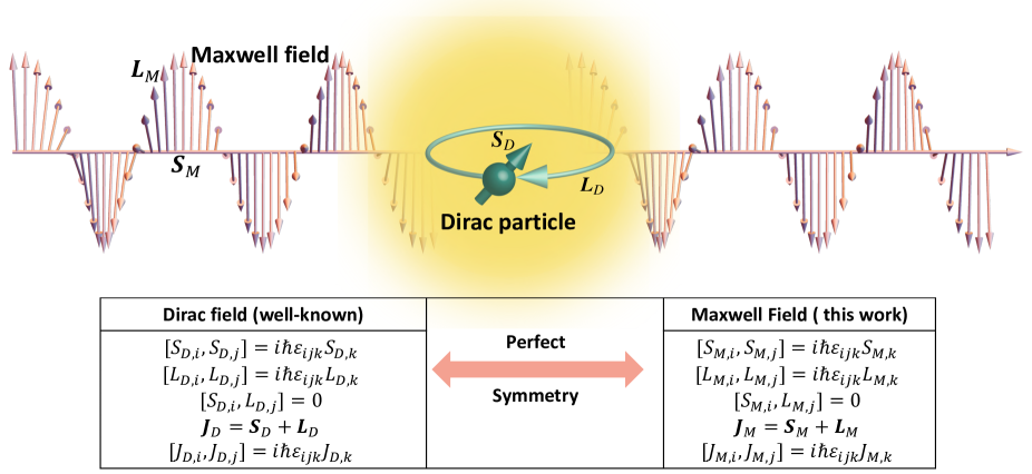
Figure 1: Comparison between our proposed photon angular momentum operators and the well-known Dirac field counterparts. We show that our discovered quantum operators $\bm{S}_{M}$ and $\bm{L}_{M}$ obey the canonical commutation relations in striking parallel to Dirac fermions.

The importance of the problem becomes clear on comparing to the Dirac spin operator $\bm{S}_{D}=(\hbar/2)\int d^{3}x\psi^{\dagger}\hat{\bm{\Sigma}}\psi$. These obey the canonical commutation relationships for angular momenta. However, a genuine quantum operator for the photon spin $\bm{S}_{M}$, which satisfy the standard equal-time commutation relations $[S_{M,i},S_{M,j}]=i\hbar\varepsilon_{ijk}S_{M,k}$, have never been obtained. Because of this major knowledge gap, interesting questions have been raised whether photon spin and OAM are true observable angular momenta at all [9, 8, 12, 34]. We solve this open problem within the canonical quantization framework of relativistic field theory. We explicitly derive the quantum operators for the spin $\bm{S}_{M}$ and OAM $\bm{L}_{M}$ of the photon by quantizing the electromagnetic (EM) field covariantly in the Lorenz gauge. Using relativistic field theory, we show a perfect symmetry between the angular momentum commutation relations for Dirac fermions and Maxwell bosons. We show that photon SAM and OAM operators commute with each other and are thus separately observable. This is an advance over existing knowledge since it is an important question whether the spin and OAM of light are independently observable  [9, 8].

Historically, duality symmetry of classical electromagnetism (Maxwell’s equations) in source free regions was the chosen route to understand conservation relation between the photon spin density and helicity  [35, 36, 37]. Important recent works have generalized this approach  [38, 39]. However, QED requires local U(1) gauge symmetry, to capture quantum light-matter interaction. Our work also fills this historic gap by investigating the angular-momentum conservation law of the combined Dirac-Maxwell fields. An important hallmark of our QED approach is that we obtain the well-known Dirac SAM and OAM operators simultaneously en route to our new photonic spin and OAM operators. We note that similar to the Aharonov-Bohm phase [40] where gauge fields and not electric/magnetic fields take center stage, the quantum spin operator of light also shares this characteristic of gauge field theory.

In this paper, we prove the perfect symmetry between the angular momentum of Dirac fermions and Maxwell bosons using quantum field theory. For the broad audience, we summarize our central result in a simple schematic (Figure 1). First, we report on the discovery of new SAM and OAM quantum operators for the photon. While the commutation relations of angular momenta for Dirac operators are well established, we show here that Maxwell operators obey the same striking symmetry. Our discovered operators for the photon spin ($\bm{S}_{M}$) necessarily requires the inclusion of virtual photons in QED. Table 1 shows a summary of our theoretical formalism that includes SO(3) rotational symmetry and local U(1) gauge symmetry of QED. On the other hand, the important previous framework of duality symmetry in Maxwell’s equations [12] only deals with the local spin density of transverse photons. Duality symmetry in Maxwell’s equations does not capture the global photon spin which includes real (transverse) and virtual (longitudinally polarized in vacuum) photons. In this paper, we only focus on the spin of the photon. However, we believe our results can be generalized in the future to the other massless gauge boson—the gluon [32, 41].

The perfect symmetry between Dirac and Maxwell angular momentum operators necessarily includes the subtle role of longitudinal and scalar photons which are not gauge invariant. To incorporate gauge invariance into the theoretical framework, we put forth a re-decomposition of the total angular momentum of the combined Dirac-Maxwell fields (see Tab. III). We reveal that the contribution of the photon spin from longitudinal photons is hidden from detection by the requirement of gauge invariance. The experimentally measurable part of the photon spin is its transverse-field part. The gauge field necessarily includes longitudinal and transverse fields as required by relativistic field theory - QED. This leads to new commutation relations for the observable total angular momentum of the photon ($[J^{\rm obs}_{M,i},J^{\rm obs}_{M,j}]=i\hbar\varepsilon_{ijk}L^{\rm obs}_{M,k}$). In our manuscript, we use the super-script “OBS” as opposed to the notation of gauge invariant variables. We note that the SAM and OAM operators commute. We prove that this is true for the new gauge operators as well as the well-known OAM and SAM operators. These results have implications for future experiments on photon spin noise [42] and exotic topological phases of matter [43].

	Current approach [35, 36, 37, 38, 39]	Our work
Symmetry type	Duality symmetry	SO(3) rotational symmetry	Local U(1) gauge symmetry
Symmetry transformation	$\bm{E}\rightarrow\bm{E}\cos\theta+c\bm{B}\sin\theta$ $\ \bm{B}\rightarrow\bm{B}\cos\theta-(\bm{E}/c)\sin\theta$	$\bm{x}\rightarrow R(\bm{\theta})\bm{x}$ ($R\ 3\times 3$ matrix) $\psi(\bm{x})\rightarrow e^{i\bm{J}\cdot\bm{\theta}}\psi(\bm{x})$	$A_{\mu}(x)\rightarrow A_{\mu}(x)-\partial_{\mu}f(x)$ $\psi(x)\rightarrow\psi(x)e^{iqf(x)/\hbar}$
Physical phenomenon	conservation of helicity	conservation of angular momentum	Massless photon
Involved spin angular momentum	provides local classical spin density of transverse EM field; does not lead to angular momentum commutation relations	full spin operator of the isolated photon [U(1) gauge field] satisfies the correct commutation relations	introducing interaction between Dirac-Maxwell field leads to the gauge invariant photon spin

Table 1: Our work is fundamentally beyond duality symmetry and incorporates SO(3) rotational symmetry and local U(1) gauge symmetries.

II Historical context of the quantum spin operator of the photon

To show the novelty of this work, we give a short review of the theoretical development of the photon spin in quantum optics. In Chap. I of the text book [44], the authors have shown that the total angular momentum of classical electrodynamics (CED) can be split into three parts:

$$\bm{J}_{\rm CED}=\sum_{\alpha}\bm{x}_{\alpha}\times\bm{p}_{\alpha}+\bm{S}^{\rm obs}_{M}+\bm{L}^{\rm obs}_{M}.$$ (1)

Here, the first term denotes the OAM of charge particles and $\bm{p}_{\alpha}=m_{\alpha}\dot{\bm{x}}_{\alpha}+q_{\alpha}\bm{A}_{\perp}$ is the canonical momentum of the $\alpha$th particle with charge $q_{\alpha}$ and mass $m_{\alpha}$. The subscript $\ {}_{\perp}$ of the vector potential denotes its transverse part with vanishing divergence, i.e., $\bm{\nabla}\cdot\bm{A}_{\perp}$=0. The second and third terms have been interpreted as the SAM and OAM of light, respectively,

$$\bm{S}^{\rm obs}_{M} =\varepsilon_{0}\int d^{3}x\bm{E}_{\perp}\times\bm{A}_{\perp},$$ (2)

$$\bm{L}^{\rm obs}_{M} =\varepsilon_{0}\int d^{3}xE_{\perp}^{j}(\bm{x}\times\bm{\nabla})A_{\perp}^{j}.$$ (3)

Here, we have added the superscript “obs” in $\bm{S}^{\rm obs}_{M}$ and $\bm{L}^{\rm obs}_{M}$, because we will show in later sections these are only the directly observable part of the photonic angular momenta. The total angular momenta $\bm{J}_{\rm CED}$ of CED is a conserved quantity, and all the three parts in Eq. (1) are invariant under a classical gauge transformation. Thus, the decomposition of the angular momentum of CED in free space has been completely solved.

Two fundamental problems in electrodynamics angular momentum decomposition occur after quantization. Firstly, the OAM of a charged particle $\bm{p}=-i\hbar\bm{\nabla}$ is not gauge-invariant anymore because an extra space-time-dependent phase is acquired under a gauge transformation. Secondly, the early important work by van Enk and Nienhuis has shown that the photon spin from CED does not satisfy the angular momentum commutation relation [9, 8], $[S^{\rm obs}_{M,i},S^{\rm obs}_{M,j}]=0$. Thus the open question remains whether new quantum operators exist beyond these well known classical results that satisfy the correct canonical commutation relations. In this paper, we find these SAM and OAM operators of photons using quantum field theory. Furthermore, we also derive the above well known classical decomposition through the quantum operators.

Due to these two unsolved problems and the lack of a quantum gauge theory, the conservation of photon spin has been studied  [12] only in the absence of charges using electric-magnetic duality symmetry  [11, 38, 45]. By building on Lipkin-Calkin conservation law [37, 36], the photon spin density has been previously interpreted $\bm{s}^{\rm obs}(\bm{x},t)$ as the current corresponding to the photonic helicity $h(\bm{x},t)$, i.e., $\partial h/\partial t+\bm{\nabla}\cdot\bm{s}^{\rm obs}=0$. An experiment has also been implemented to measure the photonic helicity and the related quantity photonic chirality [46]. We note that these elegant works are of broad interest, but their results do not lead to new SAM and OAM operators especially for the gauge field. Electric-magnetic duality of Maxwell’s equations is a classical symmetry which does not apply to U(1) gauge fields which are essential to QED. The duality symmetry only gives the conservation of the photon helicity, not the angular momentum of gauge fields. On the other hand, in the presence of charges (Dirac fermions), this duality symmetry will be destroyed. In QED, it has been well-accepted that the conservation of angular momentum is due to the SO(3) rotational symmetry of the background space-time. The duality-symmetry-based argument cannot be extended to explain the conservation of spin for all other particles (e.g., gluons and Dirac fermions). Therefore, we appeal to quantum field theory to discover new SAM and OAM operators and also present a unified framework for gauge-field SAM and OAM.

In the high-energy community, the separation of the total angular momentum of photons and gluons into gauge-invariant spin and orbital contributions is an important and interesting challenge faced by gauge field theories like QED and quantum chromodynamics (QCD) [32]. Deriving the angular momentum commutation relations from the basic postulated relation between the field and its canonical momentum is also of fundamental significance. Here, we solve these two fundamental problems in QED angular momentum decomposition conclusively. Our work also leads to the derivation of the angular momentum in classical electrodynamics theory from the new operators discovered within quantum gauge-field theory.

III New OAM and SAM operators for the photon

We utilize a quantum field theory framework to analyze the spin and orbital angular momentum of the photon. In quantum optics (non-relativistic QED), only the transverse degrees of freedom for the photon are quantized. In stark contrast, our relativistic treatment shows that longitudinally polarized photons are necessary to construct the full spin-1 operator for the photon. The subtle detail, overlooked previously, becomes self-evident in our starting Lagrangian that incorporates both the longitudinal part of the vector potential $\bm{A}$ and the scalar potential $A_{0}$. These quantities can not be quantized with the standard Maxwell Lagrangian density $\mathcal{L}_{M,{\rm ST}}=-F^{\mu\nu}F_{\mu\nu}/4\mu_{0}$ ($F_{\mu\nu}=\partial_{\mu}A_{\nu}-\partial_{\nu}A_{\mu}$ is the EM field tensor), because there is no canonical conjugate momentum corresponding to the scalar field $A^{0}$ and the longitudinal potential $\bm{A}_{\parallel}$ with zero curl ($\bm{\nabla}\times\bm{A}_{\parallel}=0$) has also been shown to be a redundant dynamical variable (see Chap. II in Ref. [44] ).

To obtain complete knowledge of the polarization degrees of freedom, we start from the gauge-fixed Maxwell Lagrangian density [44, 47]

$$\mathcal{L}_{M}=-(\partial_{\mu}A^{\nu})(\partial^{\mu}A_{\nu})/2\mu_{0}.$$ (4)

The covariant quantization of the photon in the Lorenz gauge can be realized by defining the canonically conjugate momentum [44, 47]

$$\pi_{\mu}=\frac{\partial\mathcal{L}_{M}}{\partial(\partial_{0}A^{\mu})}=-\frac{1}{\mu_{0}}\partial^{0}A_{\mu},$$ (5)

and postulating the fundamental equal-time commutation relations (ETCRs),

$$[A^{\mu}(\bm{x},t),\pi^{\nu}(\bm{x}^{\prime},t)] =i\hbar cg^{\mu\nu}\delta^{3}(\bm{x}-\bm{x}^{\prime}),$$ (6)

$$[A^{\mu}(\bm{x},t),A^{\nu}(\bm{x}^{\prime},t)] =[\pi^{\mu}(\bm{x},t),\pi^{\nu}(\bm{x}^{\prime},t)]=0,$$ (7)

with the metric tensor $g^{\mu\nu}=\rm{diag}\{1,-1,-1,-1\}$ of the Minkowski space and the speed of light $c=1/\sqrt{\mu_{0}\varepsilon_{0}}$ in vacuum. The photon Hamiltonian is given by

$$H_{M}=-\frac{1}{2\mu_{0}}\int d^{3}x\left[\mu_{0}^{2}\pi^{\mu}\pi_{\mu}+(\bm{\nabla}A^{\mu})\cdot(\bm{\nabla}A_{\mu})\right].$$ (8)

We note that $\pi_{\mu}$ and $A_{\mu}$ are now quantum operators. But, to highlight the spin degrees, we only add the $\hat{\ }$ symbol on the spin matrices throughout this paper.

The fundamental connection between a continuous symmetry and and the corresponding conservation law was given by Noether. Applying Noether’s theorem on the Lorentz rotation symmetry [47], we obtain the angular momentum tensor density from $\mathcal{L}_{M}$ [48](also see Appendix A),

$$M_{M}^{\mu\nu\lambda} =\Theta_{M}^{\mu\lambda}x^{\nu}-\Theta_{M}^{\mu\nu}x^{\lambda}+\frac{\partial\mathcal{L}_{M}}{\partial(\partial_{\mu}A^{\sigma})}(I^{\nu\lambda})^{\sigma\tau}A_{\tau}$$ (9)

$$=\Theta_{M}^{\mu\lambda}x^{\nu}-\Theta_{M}^{\mu\nu}x^{\lambda}-\frac{1}{\mu_{0}}[(\partial^{\mu}A^{\nu})A^{\lambda}-(\partial^{\mu}A^{\lambda})A^{\nu}]$$ (10)

where $\Theta_{M}^{\mu\lambda}$ is the energy-momentum tensor and the infinitesimal Lorentz transformation generator for the vector field is given by

$$(I^{\alpha\beta})^{\mu\nu}=g^{\alpha\mu}g^{\beta\nu}-g^{\alpha\nu}g^{\beta\mu},$$ (11)

which is a an anti-symmetric matrix $(I^{\alpha\beta})^{\mu\nu}=-(I^{\beta\alpha})^{\mu\nu}$. The first two terms in Eq. (10) comes from the spatial coordinate rotation and the last term denotes the contribution from the “intrinsic” rotation between different components of the vector potential $A_{\mu}$ [47].

Focusing on the three-dimensional rotation symmetry, we, arrive at the central result of our paper—the striking quantum operators of the spin and OAM of the photon,

$$\bm{S}_{M}=-\frac{1}{\mu_{0}c}\int d^{3}x(\partial_{0}\bm{A})\times\bm{A}=\frac{1}{c}\int d^{3}x\bm{\pi}\times\bm{A}$$ (12)

and

$$\bm{L}_{M}=\frac{1}{\mu_{0}c}\!\!\int\!\!d^{3}x(\partial_{0}A^{\mu})\bm{x}\times\bm{\nabla}A_{\mu}=-\frac{1}{c}\!\int\!\!d^{3}x\pi^{\mu}\bm{x}\times\bm{\nabla}A_{\mu},$$ (13)

from the rotations of the intrinsic and spatial degrees of freedom, respectively. Of course, given the long-standing nature of the problem, fundamental checks are required to verify these are indeed the SAM and OAM of photons. Utilizing the ETCRs in Eqs. (6) and (7), we show that our defined photon spin and OAM operators satisfy the standard angular momentum commutation relations (see Appendix B and also Appendix D)

$$[S_{M,i},S_{M,j}] =i\hbar\varepsilon_{ijk}S_{M,k},$$ (14)

$$[L_{M,i},L_{M,j}] =i\hbar\varepsilon_{ijk}L_{M,k},$$ (15)

$$[L_{M,i},S_{M,j}] =0,$$ (16)

where $\varepsilon_{ijk}$ is the three-dimensional Levi-Civita tensor and $i,j=1,2,3$. Deriving the commutation relations for the photon spin and OAM operators from the basic field ETCR ansatz (14) and (15) is of fundamental importance. This has never been achieved till date. Note the other striking result—the SAM and OAM operators of the photon commute. We also emphasize that this commutation relation can not be obtained from the standard Maxwell Lagrangian density $\mathcal{L}_{M,{\rm ST}}$ under the non-covariant quantization scheme.

It is well known that the Dirac spin operators obey SU(2) symmetry. To clearly show the SO(3) symmetry in the quantum spin degrees of the photon, we perform the plane-wave expansions on the vector potential and its canonically conjugate momentum (see Chap. 7 in Ref [47])

$$A^{\mu} =\!\!\int\!\!d^{3}k\!\sum_{\lambda=0}^{3}\!\!\sqrt{\frac{\hbar}{2\varepsilon_{0}\omega_{\bm{k}}(2\pi)^{3}}}\left[a_{\bm{k},\lambda}\epsilon^{\mu}(\bm{k},\lambda)e^{i\bm{k}\cdot\bm{x}}+\rm{h.c.}\right],$$ (17)

$$\pi^{\mu} =i\!\!\int\!\!d^{3}k\!\sum_{\lambda=0}^{3}\!\!\sqrt{\frac{\hbar\omega_{\bm{k}}}{2\mu_{0}(2\pi)^{3}}}\left[a_{\bm{k},\lambda}\epsilon^{\mu}(\bm{k},\lambda)e^{i\bm{k}\cdot\bm{x}}-\rm{h.c.}\right],$$ (18)

where $\omega_{\bm{k}}=c|\bm{k}|$ is frequency of the mode with wave vector $\bm{k}$ and the unit vectors $\epsilon(\bm{k},\lambda)$ describe the four polarization photons. Following the convention [47, 44], we let the two unit vectors $\epsilon(\bm{k},1)$ and $\epsilon(\bm{k},2)$ denote the two transverse modes, $\epsilon(\bm{k},3)=(0,\bm{k}/|\bm{k}|)$ for the longitudinal photon, and $\epsilon(\bm{k},0)=(1,0,0,0)$ for the scalar photon. In the following, we also use $\bm{\epsilon}(\bm{k},\lambda)$ to denote the spatial part of the four-vector $\epsilon(\bm{k},\lambda)$. From the ETCR ansatz in Eq. (6) and (7), we can derive the familiar bosonic commutation relations for the ladder operators $[a_{\bm{k},\lambda},a_{\bm{k}^{\prime},\lambda^{\prime}}^{\dagger}]=-g_{\lambda\lambda^{\prime}}\delta^{3}(\bm{k}-\bm{k}^{\prime})$ and $[a_{\bm{k},\lambda},a_{\bm{k}^{\prime},\lambda^{\prime}}]=[a_{\bm{k},\lambda}^{\dagger},a_{\bm{k}^{\prime},\lambda^{\prime}}^{\dagger}]=0$.

Using the plane-wave expansion, we now re-express our discovered photon spin operator (12) in an intuitive form in wave-vector space (see Appendix C)

$$\bm{S}_{M}=\hbar\int d^{3}k\phi^{\dagger}_{\bm{k}}\bm{\hat{s}}\phi_{\bm{k}},$$ (19)

where the column-vector $\phi_{\bm{k}}=[a_{\bm{k},1},a_{\bm{k},2},a_{\bm{k},3}]^{T}$ is the field operator of the photon in wave-vector space and the $3\times 3$ matrix $\bm{\hat{s}}=\sum_{\lambda=1}^{3}\hat{s}_{\lambda}\bm{\epsilon}(\bm{k},\lambda)$ is the spin-$1$ operator of the photon with the SO($3$) rotation generators

$$\hat{s}_{1}=\left[\begin{array}[]{ccc}0&0&0\\ 0&0&-i\\ 0&i&0\end{array}\right],\ \hat{s}_{2}=\left[\begin{array}[]{ccc}0&0&i\\ 0&0&0\\ -i&0&0\end{array}\right],\ \hat{s}_{3}=\left[\begin{array}[]{ccc}0&-i&0\\ i&0&0\\ 0&0&0\end{array}\right].$$ (20)

Here, we see that our defined photon spin operator generates the rotation of the polarization degrees of freedom of light.

The direction of our defined photon spin is completely determined by the polarization [i.e., the unit vector $\bm{\epsilon}(\bm{k},\lambda)$] of the photon. Thus, the spin operator indeed describes the angular momentum carried by the polarization degrees of freedom of the photon. This is significantly different from the OAM of the photon that we obtain

$$\bm{L}_{M}=i\hbar\int d^{3}k\sum_{\lambda=0}^{3}g^{\lambda\lambda}a_{\bm{k},\lambda}^{\dagger}(\bm{k}\times\bm{\nabla}_{\bm{k}})a_{\bm{k},\lambda},$$ (21)

whose direction is fully determined by the orbital motion. In Appendix C, we prove that counter-rotating wave terms $a_{\bm{k},\lambda}a_{\bm{-k},\lambda^{\prime}}$ and and $a^{\dagger}_{\bm{k},\lambda}a^{\dagger}_{\bm{-k},\lambda^{\prime}}$ both in the spin and OAM operators vanish since they change their sign when we relabel the indices $\{\bm{k},\lambda\}\rightarrow\{-\bm{k},\lambda^{\prime}\}$. We also note that different from the spin of Dirac field, the photon spin is not the intrinsic angular momentum of light, because the polarization unit vectors $\bm{\epsilon}$ are dependent on the wave vector $\bm{k}$.

There remain two subtle aspects that need further exploration for developing a full quantum theory of photon spin. Firstly, there is a fundamental requirement in QED that a measurable quantity can not change under a gauge transformation. However, both $\bm{S}_{M}$ and $\bm{L}_{M}$ defined above for the free-space photon are not gauge invariant because longitudinal and scalar photons are involved. Thus, they are not direct physical observables. We argue that this is a fundamental tenet in the construction of the correct quantum theory because additional hidden degrees of freedom are necessary to construct the above quantum spin-1 operator for the free-space photon. On the other hand, only two transverse polarizations are allowed for the photon in free space. Secondly, in the presence of charges (Dirac particles), the EM field acquires a longitudinal (near-field) component that is beyond the transverse photons commonly encountered in vacuum. Can we construct a gauge-invariant photon spin operator in the presence of charges? Next, we will answer this question conclusively and show how to incorporate the gauge invariance into the photon angular momenta.

	Dirac SAM	Dirac OAM	Maxwell SAM	Maxwell OAM
Canonical decomposition	$\bm{S}_{D}=\int d^{3}x\psi^{\dagger}\hat{\bm{\Sigma}}\psi$	$\bm{L}_{D}=\int d^{3}x\psi^{\dagger}\bm{x}\times\bm{p}\psi$	$\bm{S}_{M}=\frac{1}{c}\int d^{3}x\bm{\pi}\times\bm{A}$	$\bm{L}_{M}=-\frac{1}{c}\int d^{3}x\pi^{\mu}\bm{x}\times\bm{\nabla}A_{\mu}$
Gauge-invariant decomposition	$\bm{S}_{D}=\int d^{3}x\psi^{\dagger}\hat{\bm{\Sigma}}\psi$	$\bm{L}^{\rm obs}_{D}=\int d^{3}x\psi^{\dagger}\bm{x}\times\bm{p}\psi+\bm{L}_{\rm pure}$	$\bm{S}^{\rm obs}_{M}=\varepsilon_{0}\int d^{3}x\bm{E}_{\perp}\times\bm{A}_{\perp}$	$\bm{L}^{\rm obs}_{M}=\varepsilon_{0}\int d^{3}xE_{\perp}^{j}\bm{x}\times\bm{\nabla}A_{\perp}^{j}$
Commutation relations	$[S_{D,i},S_{D,j}]=i\hbar\varepsilon_{ijk}S_{D,k}$	$[L^{\rm obs}_{D,i},L^{\rm obs}_{D,j}]=i\hbar\varepsilon_{ijk}L^{\rm obs}_{D,k}$	$[S^{\rm obs}_{M,i},S^{\rm obs}_{M,j}]=0$	$[L^{\rm obs}_{M,i},L^{\rm obs}_{M,j}]=\hbar\varepsilon_{ijk}L^{\rm obs}_{M,k}$
	$[S_{D,i},L^{\rm obs}_{D,j}]=0$		$[S^{\rm obs}_{M,i},L^{\rm obs}_{M,j}]=0$
Total observable angular momentum	$\bm{J}^{\rm obs}_{D}=\bm{S}_{D}+\bm{L}^{\rm obs}_{D}$,$\ \ [J^{\rm obs}_{D,i},J^{\rm obs}_{D,j}]=i\hbar\varepsilon_{ijk}J^{\rm obs}_{D,k}$		$\bm{J}^{\rm obs}_{M}=\bm{S}^{\rm obs}_{M}+\bm{L}^{\rm obs}_{M}$,$\ \ [J^{\rm obs}_{M,i},J^{\rm obs}_{M,j}]=i\hbar\varepsilon_{ijk}L^{\rm obs}_{M,k}$

Table 2: Perfect vs. broken symmetry in angular momentum commutation relations of the photon: In the canonical decomposition $\bm{J}=\bm{S}_{D}+\bm{L}_{D}+\bm{S}_{M}+\bm{L}_{M}$, the four angular momenta commute with each other and all of them satisfy the angular momentum commutation relations. But three of them are not gauge invariant. In $\bm{J}=\bm{S}_{D}+\bm{L}^{\rm obs}_{D}+\bm{S}^{\rm obs}_{M}+\bm{L}^{\rm obs}_{M}$ decomposition, all the four parts are gauge invariant and they also commute with each other. The term $\bm{L}_{\rm pure}$ denotes the pure gauge contribution of the light to the Dirac orbital angular momentum (OAM), which will disappear in the Coulomb gauge. Specifically, the gauge-invariant photon SAM and OAM operators commute revealing that they are true angular momenta.

IV Gauge invariant decomposition of QED angular momentum

We now put forth a gauge invariant theoretical framework to make connections to experimentally observable OAM and SAM. We note that photons are massless gauge bosons under the local $U(1)$-gauge symmetry of the standard (subscript “ST”) QED Lagrangian density $\mathcal{L}_{\rm QED,ST}=i\hbar c\bar{\psi}\gamma^{\mu}\partial_{\mu}\psi-mc^{2}\bar{\psi}\psi-qc\bar{\psi}\gamma_{\mu}A^{\mu}\psi+\mathcal{L}_{M,{\rm ST}}$. Thus, the gauge-dependence problem can only be fully solved by a theoretical framework that combines Dirac-Maxwell fields. This line of exploration is a paradigm shift from previous approaches in the field of photonics that do not use a fundamental QED theory including Dirac particles for addressing this problem. We argue that any measurement process of photon’s SAM and OAM necessarily requires interaction with matter i.e. Dirac-Maxwell fields have to be analyzed as opposed to Maxwell fields alone. Thus, conservation laws which emerge from the combined Dirac-Maxwell-field angular momenta provides the clear path towards analyzing experimental observables. Schematically, this is depicted in Fig. 1 which deals with a relativistic quantum scattering experiment of a photon with a Dirac particle [49]. We put forth the OAM and SAM conservation laws in this set-up to develop a theoretical framework for gauge invariant SAM and OAM observables. We note that our definition of transverse and longitudinal follows the QED literature. It is unrelated to classical transverse concept defined in relation to the propagation direction for plane waves.

We first start from a gauge non-invariant QED Lagrangian density

$$\mathcal{L}_{\rm QED}=i\hbar c\bar{\psi}\gamma^{\mu}\partial_{\mu}\psi-mc^{2}\bar{\psi}\psi-qc\bar{\psi}\gamma_{\mu}A^{\mu}\psi+\mathcal{L}_{M},$$ (22)

where the gauge non-invariance arises from $\mathcal{L}_{M}$. We exploit a novel re-decomposition of the total angular momentum and enforcement of the Lorenz gauge condition to obtain the gauge-invariant SAM and OAM. To prove that our procedure is exact, we arrive at the same striking result through an alternative path where the gauge issue can be solved by quantizing the standard gauge-invariant Lagrangian density $\mathcal{L}_{\rm QED,ST}$ in the Coulomb gauge (see Appendix G).

The total angular momentum of the combined Dirac-Maxwell fields can be decomposed in two different ways which we term as canonical and gauge-invarant decomposition. Canonical decomposition: According to Noether’s theorem, the total QED angular momentum obtained from $\mathcal{L}_{\rm QED}$ contains four parts $\bm{J}=\bm{S}_{D}+\bm{L}_{D}+\bm{S}_{M}+\bm{L}_{M}$. The SAM and OAM of the photon have been given in the previous part of the work. The SAM and OAM of the Dirac field are given by $\bm{S}_{D}=\frac{1}{2}\hbar\int d^{3}x\psi^{\dagger}\hat{\bm{\Sigma}}\psi$ and $\bm{L}_{D}=-i\hbar\int d^{3}x\psi^{\dagger}\bm{x}\times\bm{\nabla}\psi$, respectively. All four parts in the canonical decomposition satisfy the angular momentum commutation relations and they commute with each other. However, except for the Dirac spin, all the other three parts in $\bm{J}$ are not gauge invariant.

Gauge-invariant decomposition: To obtain the gauge-invariant variables, we introduce the concept of gauge flow. Here, we extract the parts in $\bm{S}_{M}$ and $\bm{L}_{M}$ containing scalar and longitudinal photons and flow them into the OAM of the Dirac field $\bm{L}_{D}$. Then, we obtain the gauge-invariant decomposition of the total angular momentum (superscript “obs”):

$$\bm{S}_{D}+\bm{L}_{D}+\bm{S}_{M}+\bm{L}_{M}=\bm{J}=\bm{S}_{D}+\bm{L}^{\rm obs}_{D}+\bm{S}^{\rm obs}_{M}+\bm{L}^{\rm obs}_{M}.$$ (23)

In Tab. III, we contrast the canonical decomposition of the total QED angular momentum with this gauge invariant decomposition. The gauge invariant part of our defined photon SAM and OAM operators recovers the angular momentum of light from CED [44] $\bm{S}^{\rm obs}_{M}=\int d^{3}k\bm{s}_{\bm{k},3}=\varepsilon_{0}\!\int\!d^{3}x\bm{E}_{\perp}\!\times\!\bm{A}_{\perp}$ and $\bm{L}^{\rm obs}_{M}\!=\!-i\hbar\!\!\int\!\!d^{3}k\!\!\sum_{\lambda=1,2}a_{\bm{k},\lambda}^{\dagger}(\bm{k}\times\bm{\nabla}_{\bm{k}})a_{\bm{k},\lambda}\!=\!\varepsilon_{0}\!\!\int\!\!d^{3}xE_{\perp}^{j}\bm{x}\times\bm{\nabla}A_{\perp}^{j}$. Here, $\bm{s}_{\bm{k},3}=i\hbar(a_{\bm{k},2}^{\dagger}a_{\bm{k},1}\!-\!a_{\bm{k},1}^{\dagger}a_{\bm{k},2})\bm{\epsilon}(\bm{k},3)$ is the observable spin density in $\bm{k}$-space and we have used the relation between $\bm{\pi}$ and the electric field $\bm{E}=-c\left(\partial^{0}\bm{A}+\bm{\nabla}A^{0}\right)=c\mu_{0}\bm{\pi}-c\bm{\nabla}A^{0}$. This shows that the gauge-invariant part of the photon spin $\bm{S}^{\rm obs}_{M}$ only contains information from the propagation direction within the full plane wave expansion [see Eq. (19)]. We note that the $\bm{S}^{\rm obs}_{M}$ is not the total photon spin operator  [44] as it does not obey angular momentum commutation rules. Our result clearly shows that it is only the transverse-field sector of the total photon spin ($S_{M}$).

The hallmark of our work is that our proposed Maxwellian SAM and OAM simultaneously recovers the correct OAM and SAM of the Dirac field. The gauge-invariant OAM of the Dirac field obtained from the above analysis is

$$\bm{L}^{\rm obs}_{D}=\int d^{3}x\psi^{\dagger}\bm{x}\times(-i\hbar\bm{\nabla})\psi+\bm{L}_{\rm pure},$$ (24)

where $\bm{L}_{\rm pure}$ is the pure gauge contribution from the EM field (see Appendix E). We have verified that the mean value of $\bm{L}^{\rm obs}_{D}$ is gauge invariant.

There is another important physical observable related to circularly polarized photons and closely related to the photon spin—the photon helicity. Helicity is the magnitude of spin projection on the propagating direction of the particle, which is a Lorentz invariant scalar. Because only $\bm{S}^{\rm obs}_{M}$ has components in $\bm{k}$-direction, thus the photon helicity is given by

$$\Lambda_{M} =\int d^{3}k\frac{\bm{s}_{\bm{k},3}\cdot\bm{k}}{|\bm{k}|}=i\hbar\int d^{3}k(a_{\bm{k},2}^{\dagger}a_{\bm{k},1}\!-\!a_{\bm{k},1}^{\dagger}a_{\bm{k},2}).$$ (25)

We argue that our decomposition $\bm{J}=\bm{S}_{D}+\bm{L}^{\rm obs}_{D}+\bm{S}^{\rm obs}_{M}+\bm{L}^{\rm obs}_{M}$ embodies the correct physical behavior of QED angular momentum. We arrive at two new fundamental commutation relations for OAM of the Dirac fields as well as Maxwell fields

$$[L^{\rm obs}_{D,i},L^{\rm obs}_{D,j}] =i\hbar\varepsilon_{ijk}L_{D,k}^{\rm obs},$$ (26)

$$[L_{M,i}^{\rm obs},L_{M,j}^{\rm obs}] =i\hbar\varepsilon_{ijk}L_{M,k}^{\rm obs}.$$ (27)

We note the perfect symmetry once again proving that experimentally observable OAM for Dirac-Maxwell fields follows the uncertainty principle.

The definition of the Dirac spin is in agreement with previous literature, which certainly satisfies the standard angular momentum commutation relation $[S_{D,i},S_{D,j}]=i\hbar\varepsilon_{ijk}S_{D,k}$. However, the observable (gauge-invariant) photon spin operators do not obey the above mentioned symmetry of the full photon spin operator. As shown previously [9, 8], the components of the transverse-field photon spin commute with each other

$$[S^{\rm obs}_{M,i},S^{\rm obs}_{M,j}]=0.$$ (28)

The fundamental reason is because this latter observable spin operator does not contain the contribution from longitudinally polarized photons i.e. virtual photons. We emphasize that the full spin operators for Dirac-Maxwell fields obtained by us exhibits the perfect symmetry (Fig. 1).

	Dirac SAM	Dirac OAM	Maxwell SAM	Maxwell OAM	Quantized independent observables
Our Decomposition	$\frac{1}{2}\hbar\!\int\!d^{3}x\psi^{\dagger}\hat{\bm{\Sigma}}\psi$	$\int\!d^{3}x\psi^{\dagger}\bm{x}\times\bm{p}\psi\!+\!\bm{L}_{\rm pure}$	$\varepsilon_{0}\!\!\int\!\!d^{3}x\bm{E}_{\perp}\!\!\times\!\!\bm{A}_{\perp}$	$\varepsilon_{0}\int d^{3}xE_{\perp}^{j}\bm{x}\times\bm{\nabla}A_{\perp}^{j}$	Yes
Belinfante [26] Decomposition	$\bm{J}_{D}=\!\!\int\!\!d^{3}x\bar{\psi}[\bm{x}\times\frac{1}{2}(\gamma^{0}i\bm{D}+\bm{\gamma}iD^{0})]\psi$		$\bm{J}_{M}=\varepsilon_{0}\!\int d^{3}x\bm{x}\times(\bm{E}\times\bm{B})$		No
Ji  [28] Decomposition	$\frac{1}{2}\hbar\!\int\!d^{3}x\psi^{\dagger}\hat{\bm{\Sigma}}\psi$	$\frac{1}{2}\hbar\!\int\!d^{3}x\psi^{\dagger}\bm{x}\times i\bm{D}\psi$	$\bm{J}_{M}=\varepsilon_{0}\!\int d^{3}x\bm{x}\times(\bm{E}\times\bm{B})$		No
Jaffe-Manohar [27] Decomposition	$\frac{1}{2}\hbar\!\int\!d^{3}x\psi^{\dagger}\hat{\bm{\Sigma}}\psi$	$\int d^{3}x\psi^{\dagger}\bm{x}\times\bm{p}\psi$	$\varepsilon_{0}\!\int\!d^{3}x\bm{E}\!\times\!\bm{A}$	$\varepsilon_{0}\int d^{3}xE^{j}\bm{x}\times\bm{\nabla}A^{j}$	No
Chen et al [29] Decomposition	$\frac{1}{2}\hbar\!\int\!d^{3}x\psi^{\dagger}\hat{\bm{\Sigma}}\psi$	$\int\!d^{3}x\psi^{\dagger}\bm{x}\!\times\!(\bm{p}\!-\!q\bm{A}_{\parallel})\psi$	$\varepsilon_{0}\!\int\!d^{3}x\bm{E}\!\times\!\bm{A}_{\perp}$	$\varepsilon_{0}\int d^{3}xE^{j}\bm{x}\times\bm{\nabla}A_{\perp}^{j}$	No
Wakamatsu [30] Decomposition	$\frac{1}{2}\hbar\!\int\!d^{3}x\psi^{\dagger}\hat{\bm{\Sigma}}\psi$	$\int\!d^{3}x\psi^{\dagger}\bm{x}\times(\bm{p}\!-\!q\bm{A})\psi$	$\varepsilon_{0}\!\int\!d^{3}x\bm{E}\!\times\!\bm{A}_{\perp}$	$\varepsilon_{0}\int d^{3}x[E^{j}\bm{x}\times\!\bm{\nabla}A_{\perp}^{j}+\!(\bm{\nabla}\cdot\bm{E})\bm{x}\times\bm{\nabla}\bm{A}_{\perp}]$	No

Table 3: We contrast our gauge-invariant decomposition of the QED angular momentum with previous important results that have inspired us to discover new operators (please refer to Appendix H for more details). Our work includes the role of virtual photons which is a fundamental tenet for observing symmetry between Dirac and Maxwell fields. This goes beyond the traditional QED Lagrangian density used in previous work. Furthermore, our proposed four angular momentum operators commute with each other (see Appendix F), thus they can be measured independently. Here, $D_{\mu}=\partial_{\mu}+iqA_{\mu}$ is the covariant derivative.

As shown in Table 3, our work marks a departure from previous decompositions [27, 28, 29, 30]. The four parts in the gauge-invariant decomposition of $\bm{J}$ [right-hand-side of equation (23)] can be measured independently in experiment. This is true since these operators commute with each other. Specifically, we rigorously prove that the observable parts of the spin and OAM of light commute (see Appendix F), i.e.,

$$[L^{\rm obs}_{M,i},S^{\rm obs}_{M,j}]=0.$$ (29)

We note that the (gauge-invariant) observable part of the total photon angular momentum $\bm{J}^{\rm obs}_{M}=\bm{L}^{\rm obs}_{M}+\bm{S}^{\rm obs}_{M}$ does not generate the rotations in space. Thus it is distinct from the total full quantum angular momentum $\bm{J}_{M}=\bm{L}_{M}+\bm{S}_{M}$. We rigorously prove that the observable total angular momentum operator leads to fundamentally new angular momentum commutation relations, i.e., $[J^{\rm obs}_{M,i},J^{\rm obs}_{M,j}]=i\hbar\varepsilon_{ijk}L^{\rm obs}_{M,k}\neq i\hbar\varepsilon_{ijk}J^{\rm obs}_{M,k}$.

Recently the photonic spin density has been directly measured through interaction of light with a room temperature quantum magnetometer [50]. Nitrogen vacancy (NV) centers in diamond function as spin qubits which are sensitive to magnetic fields as well as magnetic field fluctuations. It was shown that a detuned laser beam which is circularly polarized creates energy level shifts in the ground spin states of an NV center that are analogous to an effective static magnetic field. The experiment shows a coherent interaction between the local spin density vector and the NV center which is read out using the Ramsey interference protocol. We note that the specific physical quantity which is being measured in this experiment is the observable photonic spin density vector ($\bm{S}^{\rm obs}_{M}$). One future possibility is for this same experiment to be extended to vector magnetometry using an OAM beam or pulse. In the plane perpendicular to the propagating axis, the mean values of both the photon spin and OAM vanish. However, their quantum uncertainties are not zero [51]. Thus, the Heisenberg’s uncertainty relations for photonic OAM operators can be verified by measuring their quantum fluctuations in orthogonal directions. This vector measurement is possible through the relative alignment of the NV axis and the incident light beam. Low temperatures will be needed to extend the coherence time of the NV center to increase the sensitivity and measure both mean values and fluctuations of the observable photonic spin density vector. Therefore local photonic spin density and spin noise can be measured via a nitrogen-vacancy (NV) center, which functions as a nano-scale photonic spin density sensor [50]. Along similar lines, the orbital photogalvanic effect [52, 53] could be exploited to measure the photonic OAM density and quantum fluctuations of OAM in the transverse plane [51].

V Conclusion

We have discovered the quantum operator of the photon spin providing the first QED theory of angular momentum. Our approach involves Dirac-Maxwell fields in a quantum gauge theory framework. We have proven a perfect symmetry between the Dirac and Maxwell quantum spin operator commutation relations. In experiment, our theory can be verified through interaction of photonic spin density with an NV center [50] and the interaction of OAM density with two-dimensional materials [52, 53].

This work is supported by the funding from DARPA Nascent Light-Matter Interactions. L.P.Y has also been funded by National Key R&D Program of China (Grant No. 2021YFE0193500).

Appendix A Angular momentum of light from Noether’s theorem

To obtain enough polarization degrees of freedom to construct the full photon spin operator, we use the following Maxwell Lagrangian density to quantize the electromagnetic (EM) field in the Lorenz gauge covariantly [44, 47],

$$\mathcal{L}_{M}=-\frac{1}{2\mu_{0}}(\partial_{\mu}A^{\nu})(\partial^{\mu}A_{\nu}).$$ (30)

We note that, different from the standard EM Lagrangian density $\mathcal{L}_{M,{\rm ST}}=-(1/4\mu_{0})F^{\mu\nu}F_{\mu\nu}$, $\mathcal{L}_{M}$ itself is not gauge invariant. We will show how to eliminate the gauge dependence in the physical quantities via the gauge condition in the following.

These two Lagrangian density $\mathcal{L}_{M}$ and $\mathcal{L}_{M,{\rm ST}}$ can be connected via [47, 44]

$$\mathcal{L}_{M}=\mathcal{L}_{M,{\rm ST}}-\frac{1}{2}(\partial_{\mu}A^{\mu})^{2}+\frac{1}{2}\partial_{\mu}[A_{\nu}(\partial^{\nu}A^{\mu})-(\partial_{\nu}A^{\nu})A^{\mu}].$$ (31)

The last four divergence term can be dropped since the EM fields are assumed to tend to 0 sufficiently fast at infinity. Under the Lorenz gauge condition $\partial_{\mu}A^{\mu}=0$, these two Lagrangian densities are equivalent to each other.

Noether’s theorem tells us that if the action $W=\int d^{4}x\mathcal{L}$ keeps invariant under a continuous symmetry transformation, a conserved quantity can be obtained (see Chap.2 in Ref. [47]). Applying the Noether’s theorem to the translation symmetry, we obtain the canonical energy-momentum tensor

$$\Theta_{M}^{\mu\nu} =\frac{\partial\mathcal{L}_{M}}{\partial(\partial_{\mu}A_{\sigma})}\partial^{\nu}A_{\sigma}-g^{\mu\nu}\mathcal{L}_{M}$$ (32)

$$=-\frac{1}{\mu_{0}}(\partial^{\mu}A^{\sigma})(\partial^{\nu}A_{\sigma})+\frac{1}{2\mu_{0}}g^{\mu\nu}(\partial^{\rho}A^{\sigma})(\partial_{\rho}A_{\sigma}).$$ (33)

This leads to the conserved four-momentum vector

$$P^{\nu}_{M}\!=\!\Theta_{M}^{0,\nu}\!=\!-\frac{1}{\mu_{0}}(\partial^{0}A^{\sigma})(\partial^{\nu}A_{\sigma})\!+\!\frac{1}{2\mu_{0}}g^{0\nu}(\partial^{\rho}A^{\sigma})(\partial_{\rho}A_{\sigma}).$$ (34)

The time component of $P^{\nu}_{M}$ gives the Hamiltonian (energy) of the system $H_{M}=P^{0}_{M}=\int d^{3}x\mathcal{H}_{M}$, with Hamiltonian density

$$\mathcal{H}_{M} =-\frac{1}{2\mu_{0}}\left[(\partial^{0}A^{\sigma})(\partial^{0}A_{\sigma})+(\bm{\nabla}A^{\sigma})\cdot(\bm{\nabla}A_{\sigma})\right].$$ (35)

The spatial part of $P^{\nu}_{M}$ gives the momentum of the EM field

$$\bm{P}_{M}=\varepsilon_{0}\int d^{3}x\dot{A}^{\sigma}\bm{\nabla}A_{\sigma},$$ (36)

where we have divided an extra constant $c$ to get the correct dimension.

Similarly, applying Noether’s theorem to the three-dimensional rotation symmetry [47], we obtain the angular momentum tensor density

$$M_{M}^{\mu\nu\lambda} =\Theta_{M}^{\mu\lambda}x^{\nu}-\Theta_{M}^{\mu\nu}x^{\lambda}+\frac{\partial\mathcal{L}_{M}}{\partial(\partial_{\mu}A^{\sigma})}(I^{\nu\lambda})^{\sigma\tau}A_{\tau}$$ (37)

where infinitesimal generator of the Lorentz group for the vector field is given by

$$(I^{\alpha\beta})^{\mu\nu}=g^{\alpha\mu}g^{\beta\nu}-g^{\alpha\nu}g^{\beta\mu}.$$ (38)

This generator is a an antisymmetric matrix

$$(I^{\alpha\beta})^{\mu\nu}=-(I^{\beta\alpha})^{\mu\nu}.$$ (39)

Utilizing $\Theta_{M}^{\mu\nu}$ and $\mathcal{L}_{M}$, we have

$$M_{M}^{\mu\nu\lambda}\! =\!\Theta_{M}^{\mu\lambda}x^{\nu}\!-\!\Theta_{M}^{\mu\nu}x^{\lambda}\!-\!\frac{1}{\mu_{0}}(\partial^{\mu}A_{\sigma})(g^{\nu\sigma}g^{\lambda\tau}\!-\!g^{\nu\tau}g^{\lambda\sigma})A_{\tau}$$ (40)

$$=\Theta_{M}^{\mu\lambda}x^{\nu}-\Theta_{M}^{\mu\nu}x^{\lambda}-\frac{1}{\mu_{0}}[(\partial^{\mu}A^{\nu})A^{\lambda}-(\partial^{\mu}A^{\lambda})A^{\nu}].$$ (41)

The total angular momentum $M_{M}^{ij}$ can be obtained from the angular momentum density $M_{M}^{\mu\nu\lambda}$ by setting $\mu=0$ and taking spatial components of $\nu$ and $\lambda$. Here, we split the total angular momentum into two parts. The first one denotes the OAM of light $L_{M}^{ij}=\int d^{3}x(\Theta_{M}^{0j}x^{i}-\Theta_{M}^{0i}x^{j})$ and the second part describes the ”intrinsic” angular momentum (the spin) of the vector field $S_{M}^{ij}=-\frac{1}{\mu_{0}}\int d^{3}x[(\partial^{0}A^{i})A^{j}-(\partial^{0}A^{j})A^{i}]$, with $i,j=x,y,z$. It is straightforward to see that, in terms of three-vectors with relation $J_{M}^{k}=\frac{1}{2}\epsilon^{ijk}M^{ij}$ [47], the OAM and SAM of light can be rewritten as

$$\bm{L}_{M} =\frac{1}{\mu_{0}c}\int d^{3}x(\partial_{0}A^{\mu})\bm{x}\times\bm{\nabla}A_{\mu},$$ (42)

$$\bm{S}_{M} =-\frac{1}{\mu_{0}c}\int d^{3}x[(\partial_{0}\bm{A})\times\bm{A}].$$ (43)

Appendix B Quantum commutation relations for angular momenta

We now show how to obtain the standard quantum commutation relations for the angular momentum of light within the canonical quantization framework. We first define the canonical conjugate momentum of light

$$\pi_{\mu}=\frac{\partial\mathcal{L}_{M}}{\partial(\partial_{0}A^{\mu})}=-\frac{1}{\mu_{0}}\partial^{0}A_{\mu}.$$ (44)

Then, we can re-write the Hamiltonian, SAM, and OAM of the photon as

$$H_{M} =-\frac{1}{2\mu_{0}}\int d^{3}x\left[\mu_{0}^{2}\pi^{\mu}\pi_{\mu}+(\bm{\nabla}A^{\mu})\cdot(\bm{\nabla}A_{\mu})\right],$$ (45)

$$\bm{S}_{M} =\frac{1}{c}\int d^{3}x\bm{\pi}\times\bm{A},$$ (46)

$$\bm{L}_{M} =-\frac{1}{c}\int d^{3}x\pi^{\mu}\bm{x}\times\bm{\nabla}A_{\mu}$$ (47)

The EM field is quantized by postulating the equal-time commutation relations,

$$[A^{\mu}(\bm{x},t),\pi^{\nu}(\bm{x}^{\prime},t)] =i\hbar cg^{\mu\nu}\delta^{3}(\bm{x}-\bm{x}^{\prime}),$$ (48)

$$[A^{\mu}(\bm{x},t),A^{\nu}(\bm{x}^{\prime},t)] =[\pi^{\mu}(\bm{x},t),\pi^{\nu}(\bm{x}^{\prime},t)]=0.$$ (49)

We now verify the canonical angular momentum commutation relations

$$[L_{M,i},L_{M,j}]= \frac{1}{c^{2}}\int d^{3}x\int d^{3}x^{\prime}[\pi_{m}(\bm{x})(\bm{x}\times\bm{\nabla})_{i}A_{m}(\bm{x}),\pi_{m^{\prime}}(\bm{x}^{\prime})(\bm{x}^{\prime}\times\bm{\nabla}^{\prime})_{j}A_{m^{\prime}}(\bm{x}^{\prime})]$$

$$= -\frac{i\hbar}{c}\!\int\!\!d^{3}x\!\!\int\!\!d^{3}x^{\prime}\left\{\pi_{m}(\bm{x}^{\prime})(\bm{x}^{\prime}\times\bm{\nabla}^{\prime})_{j}\delta^{3}(\bm{x}-\bm{x}^{\prime})(\bm{x}\times\bm{\nabla})_{i}A_{m}(\bm{x})-\pi_{m}(\bm{x})(\bm{x}\times\bm{\nabla})_{i}\delta^{3}(\bm{x}-\bm{x}^{\prime})(\bm{x}^{\prime}\times\bm{\nabla}^{\prime})_{j}A_{m}(\bm{x}^{\prime})\right\}$$ (50)

$$= -\frac{i\hbar}{c}\int d^{3}x\left\{\pi_{m}(\bm{x})(\bm{x}\times\bm{\nabla})_{j}(\bm{x}\times\bm{\nabla})_{i}A_{m}(\bm{x})-\pi_{m}(\bm{x})(\bm{x}\times\bm{\nabla})_{i}(\bm{x}\times\bm{\nabla})_{j}A_{m}(\bm{x})\right\}$$ (51)

$$= -\frac{i\hbar}{c}\int d^{3}x\left\{\pi_{m}(\bm{x})\varepsilon_{ijk}(\bm{x}\times\bm{\nabla})_{k}A_{m}(\bm{x})\right\}=i\hbar\varepsilon_{ijk}L_{M,k},$$ (52)

$$[S_{M,i},S_{M,j}]= \frac{1}{c^{2}}\varepsilon_{ikl}\varepsilon_{jk^{\prime}l^{\prime}}\int d^{3}x\int d^{3}x^{\prime}[\pi_{k}(\bm{x})A_{l}(\bm{x}),\pi_{k^{\prime}}(\bm{x}^{\prime})A_{l^{\prime}}(\bm{x}^{\prime})]$$ (53)

$$= \frac{1}{c^{2}}\varepsilon_{ikl}\varepsilon_{jk^{\prime}l^{\prime}}\int d^{3}x\int d^{3}x^{\prime}\left\{\pi_{k}(\bm{x})[A_{l}(\bm{x}),\pi_{k^{\prime}}(\bm{x}^{\prime})]A_{l^{\prime}}(\bm{x}^{\prime})+\pi_{k^{\prime}}(\bm{x}^{\prime})[\pi_{k}(\bm{x}),A_{l^{\prime}}(\bm{x}^{\prime})]A_{l}(\bm{x})\right\}$$ (54)

$$= -\frac{i\hbar}{c}d^{3}x\left[\varepsilon_{ikl}\varepsilon_{jll^{\prime}}\pi_{k}(\bm{x})A_{l^{\prime}}(\bm{x})-\varepsilon_{ikl}\varepsilon_{jk^{\prime}k}\pi_{k^{\prime}}(\bm{x})A_{l}(\bm{x})\right]=i\hbar\varepsilon_{ijk}S_{M,k},$$ (55)

$$[L_{M,i},S_{M,j}]= -\frac{1}{c^{2}}\int d^{3}x\int d^{3}x^{\prime}[\pi_{m}(\bm{x})(\bm{x}\times\bm{\nabla})_{i}A_{m}(\bm{x}),\varepsilon_{jkl}\pi_{k}(\bm{x}^{\prime})A_{l}(\bm{x}^{\prime})]$$ (56)

$$= \frac{i\hbar}{c}\varepsilon_{0}\int d^{3}x\int d^{3}x^{\prime}\varepsilon_{jkl}\left\{\pi_{k}(\bm{x})(\bm{x}\times\bm{\nabla})_{i}\delta^{3}(\bm{x}-\bm{x}^{\prime})A_{l}(\bm{x}^{\prime})-\pi_{k}(\bm{x}^{\prime})\delta^{3}(\bm{x}-\bm{x}^{\prime})(\bm{x}\times\bm{\nabla})_{i}A_{l}(\bm{x})\right\}$$ (57)

$$= -\frac{i\hbar}{c}\varepsilon_{0}\int d^{3}x\int d^{3}x^{\prime}\varepsilon_{jkl}\left\{\left[(\bm{x}\times\bm{\nabla})_{i}\pi_{k}(\bm{x})\right]A_{l}(\bm{x})+\pi_{k}(\bm{x})(\bm{x}\times\bm{\nabla})_{i}A_{l}(\bm{x})\right\}$$ (58)

$$= -\frac{i\hbar}{c}\varepsilon_{0}\int d^{3}x\int d^{3}x^{\prime}\varepsilon_{jkl}\left\{-\pi_{k}(\bm{x})(\bm{x}\times\bm{\nabla})_{i}A_{l}(\bm{x})+\pi_{k}(\bm{x})(\bm{x}\times\bm{\nabla})_{i}A_{l}(\bm{x})\right\}=0,$$ (59)

where we have used the partial integral techniques and the identities

$$\varepsilon_{ikm}\varepsilon_{jlm}=\delta_{ij}\delta_{kl}-\delta_{il}\delta_{km}.$$ (60)

Appendix C Key role of longitudinal degrees of freedom

To clearly show the role of polarization degrees of the Maxwell fields, we perform the plane-wave expansions to the field operators as given in Eqs. (17) and (18). The plane-wave expansion of the Dirac field has been well studied. Here, we mainly focus on the expansion of the SAM and OAM of photons. The polarization unit vectors in Eqs. (17) and (18) satisfy the four-dimensional orthonormal conditions

$$\epsilon_{\mu}(\bm{k},\lambda)\epsilon^{\mu}(\bm{k},\lambda^{\prime})=g_{\lambda\lambda^{\prime}}.$$ (61)

and the covariant completeness relation [47]

$$\sum_{\lambda=0}^{3}g_{\lambda\lambda}\epsilon_{\mu}(\bm{k},\lambda)\epsilon_{\nu}(\bm{k},\lambda)=g_{\mu\nu},$$ (62)

where $g_{\lambda\lambda}$ at the left hand side denotes the sign $\pm 1$ instead of the metric tensor. Here, we emphasize that the plane-wave expansion of $\pi^{\mu}$ is not obtained via the relation in Eq. (44). Equations (17) and (18) function more like the definition of the ladder operators. We note that the photonic angular momentum relations in Eqs. (14-16) can also be verified via their plane-wave expansions in the $\bm{k}$-space as shown in Appendix D.

We can re-express the ladder operators $a_{\bm{k},\lambda}$ and $a_{\bm{k},\lambda}^{\dagger}$ with canonical field variables $A^{\mu}$ and $\pi^{\mu}$ via the inverse transformation

$$a_{\bm{k},\lambda} =g_{\lambda\lambda}\!\!\int\!\!d^{3}x\sqrt{\frac{\varepsilon_{0}}{2\hbar\omega_{\bm{k}}(2\pi)^{3}}}\left[\omega_{\bm{k}}A^{\mu}(\bm{x})-\frac{i}{\varepsilon_{0}}\pi^{\mu}(\bm{x})\right]\epsilon_{\mu}(\bm{k},\lambda)e^{-i\bm{k}\cdot\bm{x}},$$ (63)

$$a_{\bm{k},\lambda}^{\dagger} =g_{\lambda\lambda}\int d^{3}x\sqrt{\frac{\varepsilon_{0}}{2\hbar\omega_{\bm{k}}(2\pi)^{3}}}\left[\omega_{\bm{k}}A^{\mu}(\bm{x})+\frac{i}{\varepsilon_{0}}\pi^{\mu}(\bm{x})\right]\epsilon_{\mu}(\bm{k},\lambda)e^{i\bm{k}\cdot\bm{x}}.$$ (64)

Utilizing the quantization ansatz (48) and (49) for the photon, we can verify that the ladder operators satisfy the bosonic commutations

$$[a_{\bm{k},\lambda},a_{\bm{k}^{\prime},\lambda^{\prime}}^{\dagger}] =-g_{\lambda\lambda^{\prime}}\delta^{3}(\bm{k}-\bm{k}^{\prime}),$$ (65)

$$[a_{\bm{k},\lambda},a_{\bm{k}^{\prime},\lambda^{\prime}}] =[a_{\bm{k},\lambda}^{\dagger},a_{\bm{k}^{\prime},\lambda^{\prime}}^{\dagger}]=0.$$ (66)

The plane-wave expansion of the Hamiltonian $H_{M}$ and the momentum $\bm{P}_{M}$ of the photon have been given in the textbook [47, 44]. Here, we give some details,

$$H_{M}= \int d^{3}x\mathcal{H}_{M}=-\frac{1}{2}\int\left(\mu_{0}\pi^{\mu}\pi_{\mu}+\frac{1}{\mu_{0}}(\bm{\nabla}A^{\mu})\cdot(\bm{\nabla}A_{\mu})\right)d^{3}x$$

$$= -\!\!\!\int\!\!d^{3}x\!\!\!\int\!\!d^{3}k\!\!\!\int\!\!d^{3}k^{\prime}\!\sum_{\lambda\lambda^{\prime}}\frac{\hbar}{4(2\pi)^{3}\sqrt{\omega_{\bm{k}}\omega_{\bm{k}^{\prime}}}}\epsilon^{\mu}(\bm{k},\lambda)\epsilon_{\mu}(\bm{k}^{\prime},\lambda^{\prime})$$

$$\!\!\!\!\times\left(\omega_{\bm{k}}\omega_{\bm{k}^{\prime}}\!+\!c^{2}\bm{k}\cdot\bm{k}^{\prime}\right)\left[a_{\bm{k},\lambda}a_{\bm{k}^{\prime},\lambda^{\prime}}^{\dagger}e^{-i(k-k^{\prime})\cdot x}\!+\!a_{\bm{k},\lambda}^{\dagger}a_{\bm{k}^{\prime},\lambda^{\prime}}e^{i(k-k^{\prime})\cdot x}\right.$$

$$\left.-a_{\bm{k},\lambda}a_{\bm{k}^{\prime},\lambda^{\prime}}e^{-i(k+k^{\prime})\cdot x}-a_{\bm{k},\lambda}^{\dagger}a_{\bm{k}^{\prime},\lambda^{\prime}}^{\dagger}e^{i(k+k^{\prime})\cdot x}\right]$$

$$= -\!\!\int\!vd^{3}k\frac{\hbar\omega_{\bm{k}}}{2}\!\sum_{\lambda\lambda^{\prime}}\epsilon^{\mu}(\bm{k},\lambda)\epsilon_{\mu}(\bm{k},\lambda^{\prime})\left(a_{\bm{k},\lambda}a_{\bm{k},\lambda^{\prime}}^{\dagger}\!+\!a_{\bm{k},\lambda}^{\dagger}a_{\bm{k},\lambda^{\prime}}\right)$$

$$= -\frac{1}{2}\int d^{3}k\hbar\omega_{\bm{k}}\sum_{\lambda}g_{\lambda\lambda}\left(a_{\bm{k},\lambda}a_{\bm{k},\lambda}^{\dagger}+a_{\bm{k},\lambda}^{\dagger}a_{\bm{k},\lambda}\right)$$ (67)

$$= \!\!\int\!\!d^{3}k\hbar\omega_{\bm{k}}\left(a_{\bm{k},1}^{\dagger}a_{\bm{k},1}\!+\!a_{\bm{k},2}^{\dagger}a_{\bm{k},2}\!+\!a_{\bm{k},3}^{\dagger}a_{\bm{k},3}\!-\!a_{\bm{k},0}^{\dagger}a_{\bm{k},0}\right),$$ (68)

where the normal-ordering has been taken in the last step. We note that the counter-rotating wave terms (i.e., $a_{\bm{k},\lambda}a_{\bm{k}^{\prime},\lambda^{\prime}}$ and $a_{\bm{k},\lambda}^{\dagger}a^{\dagger}_{\bm{k}^{\prime},\lambda^{\prime}}$) vanish due to $(\omega_{\bm{k}}\omega_{\bm{k}^{\prime}}+c^{2}\bm{k}\cdot\bm{k}^{\prime})=0$ when $\bm{k}=-\bm{k}^{\prime}$. No rotating wave approximation has been taken here.

We also note that there are three main problems in the covariant quantization in the Lorenz gauge: (1) the Hamiltonian is not gauge invariant; (2) the frequency of the scalar photon is negative; (3) the norm of the scalar-photon state can be negative, i.e., $\langle 0|a_{\bm{k},0}a_{\bm{k},0}^{\dagger}|0\rangle=-1$. The first two problems can be solved simultaneously by enforcing the Gupta-Bleuler constraint  [54, 55], which is the quantum version of the Lorenz gauge condition. This gauge condition is essential to obtain the quantum Maxwell equation and to remove the gauge dependence in the Lorenz-gauge quantization framework. The last problem can be solved by exploiting Dirac’s indefinite metric in space of quantum states [56, 54, 55] (also see Chap. V in the book [44]).

Similarly, the momentum of the EM field is expanded as

$$\bm{P}_{M} =\varepsilon_{0}\int d^{3}x\dot{A}^{\sigma}\bm{\nabla}A_{\sigma}=-\frac{1}{c}\int d^{3}x\pi^{\mu}\bm{\nabla}A_{\mu}$$ (69)

$$\!=\!\!\int\!\!d^{3}k\left(a_{\bm{k},1}^{\dagger}a_{\bm{k},1}\!+\!a_{\bm{k},2}^{\dagger}a_{\bm{k},2}\!+\!a_{\bm{k},3}^{\dagger}a_{\bm{k},3}\!-\!a_{\bm{k},0}^{\dagger}a_{\bm{k},0}\right)\hbar\bm{k}.$$ (70)

In the plane-wave expansion of $\bm{P}_{M}$, fast-oscillating counter-rotating wave terms also cancel out with each other, i.e.,

$$\frac{1}{2}\sum_{\lambda\lambda^{\prime}}\int d^{3}k\hbar\bm{k}a_{\bm{k},\lambda}a_{-\bm{k},\lambda^{\prime}}\epsilon^{\mu}(\bm{k},\lambda)\epsilon_{\mu}(-\bm{k},\lambda^{\prime})$$

$$= \frac{1}{4}\sum_{\lambda\lambda^{\prime}}\int d^{3}k\hbar\bm{k}(a_{\bm{k},\lambda}a_{-\bm{k},\lambda^{\prime}}+a_{\bm{-k},\lambda^{\prime}}a_{\bm{k},\lambda})\epsilon^{\mu}(\bm{k},\lambda)\epsilon_{\mu}(-\bm{k},\lambda^{\prime})$$

$$= \frac{1}{4}\sum_{\lambda\lambda^{\prime}}\int d^{3}k\hbar\bm{k}a_{\bm{k},\lambda}a_{-\bm{k},\lambda^{\prime}}[\epsilon^{\mu}(\bm{k},\lambda)\epsilon_{\mu}(-\bm{k},\lambda^{\prime})$$

$$-\epsilon^{\mu}(-\bm{k},\lambda^{\prime})\epsilon_{\mu}(\bm{k},\lambda)]=0,$$ (71)

where we have used the property $[a_{\bm{k},\lambda},a_{-\bm{k},\lambda^{\prime}}]=0$ and the four-vector inner product does not dependent on the order of the two vectors. Similar argument shows that $a^{\dagger}_{\bm{k}\lambda},a^{\dagger}_{-\bm{k},\lambda^{\prime}}$ terms also vanish.

The SAM of the Maxwell field can be expanded as

$$\bm{S}_{M}= -\frac{1}{\mu_{0}c}\int d^{3}x(\partial_{0}\bm{A})\times\bm{A}=\frac{1}{c}\int d^{3}x\bm{\pi}\times\bm{A}$$ (72)

$$= \frac{i\hbar}{2(2\pi)^{3}}\!\!\int\!\!d^{3}k\!\!\int\!\!d^{3}k^{\prime}\!\!\int\!\!d^{3}x\!\sum_{\lambda,\lambda^{\prime}=1}^{3}\sqrt{\frac{\omega_{\bm{k}}}{\omega_{\bm{k}^{\prime}}}}\left[a_{\bm{k},\lambda}\bm{\epsilon}(\bm{k},\lambda)e^{i\bm{k}\cdot\bm{x}}\!-\!a_{\bm{k},\lambda}^{\dagger}\bm{\epsilon}(\bm{k},\lambda)e^{-i\bm{k}\cdot\bm{x}}\right]\left[a_{\bm{k}^{\prime},\lambda^{\prime}}\bm{\epsilon}(\bm{k}^{\prime},\lambda^{\prime})e^{i\bm{k^{\prime}}\cdot\bm{x}}+a_{\bm{k}^{\prime},\lambda^{\prime}}^{\dagger}\bm{\epsilon}(\bm{k},\lambda^{\prime})e^{-i\bm{k}^{\prime}\cdot\bm{x}}\right]$$ (73)

$$= i\hbar\!\!\int\!\!d^{3}k\left[\left(a_{\bm{k},3}^{\dagger}a_{\bm{k},2}\!-\!a_{\bm{k},2}^{\dagger}a_{\bm{k},3}\right)\bm{\epsilon}(\bm{k},1)\!+\!\left(a_{\bm{k},1}^{\dagger}a_{\bm{k},3}\!-\!a_{\bm{k},3}^{\dagger}a_{\bm{k},1}\right)\bm{\epsilon}(\bm{k},2)\!+\!\left(a_{\bm{k},2}^{\dagger}a_{\bm{k},1}\!-\!a_{\bm{k},1}^{\dagger}a_{\bm{k},2}\right)\bm{\epsilon}(\bm{k},3)\right]\equiv i\hbar\int d^{3}k\sum_{\lambda=1}^{3}\bm{s}_{\bm{k},\lambda},$$ (74)

with

$$\bm{s}_{\bm{k},1} =(a_{\bm{k},3}^{\dagger}a_{\bm{k},2}-a_{\bm{k},2}^{\dagger}a_{\bm{k},3})\bm{\epsilon}(\bm{k},1),$$ (75)

$$\bm{s}_{\bm{k},2} =(a_{\bm{k},1}^{\dagger}a_{\bm{k},3}-a_{\bm{k},3}^{\dagger}a_{\bm{k},1})\bm{\epsilon}(\bm{k},2),$$ (76)

$$\bm{s}_{\bm{k},3} =(a_{\bm{k},2}^{\dagger}a_{\bm{k},1}-a_{\bm{k},1}^{\dagger}a_{\bm{k},2})\bm{\epsilon}(\bm{k},3).$$ (77)

Now, we show that the counter-rotating wave terms in the photon spin also vanish,

$$\frac{i\hbar}{2}\sum_{\lambda\lambda^{\prime}}\int d^{3}ka_{\bm{k},\lambda}a_{-\bm{k},\lambda^{\prime}}\bm{\epsilon}(\bm{k},\lambda)\times\bm{\epsilon}(-\bm{k},\lambda^{\prime})$$

$$= \frac{i\hbar}{4}\sum_{\lambda\lambda^{\prime}}\int d^{3}k\left[a_{\bm{k},\lambda}a_{-\bm{k},\lambda^{\prime}}+a_{-\bm{k},\lambda^{\prime}}a_{\bm{k},\lambda}\right]\bm{\epsilon}(\bm{k},\lambda)\times\bm{\epsilon}(-\bm{k},\lambda^{\prime})$$

$$= \frac{i\hbar}{4}\sum_{\lambda\lambda^{\prime}}\int d^{3}ka_{\bm{k},\lambda}a_{-\bm{k},\lambda^{\prime}}[\bm{\epsilon}(\bm{k},\lambda)\times\bm{\epsilon}(-\bm{k},\lambda^{\prime})$$

$$+\bm{\epsilon}(-\bm{k},\lambda^{\prime})\times\bm{\epsilon}(\bm{k},\lambda)]=0$$ (78)

Similar argument also applies to the terms $a^{\dagger}_{\bm{k}\lambda},a^{\dagger}_{-\bm{k},\lambda^{\prime}}$.

The Maxwell OAM can be expanded as

$$\bm{L}_{M}= \frac{1}{\mu_{0}c}\int d^{3}x(\partial_{0}A^{\mu})\bm{x}\times\bm{\nabla}A_{\mu}=-\frac{1}{c}\int d^{3}x\pi_{\mu}\bm{x}\times\bm{\nabla}A^{\mu}$$ (79)

$$= -\frac{\hbar}{2(2\pi)^{3}}\!\int\!\!d^{3}x\!\int\!\!d^{3}k\int\!\!d^{3}k^{\prime}\!\sum_{\lambda^{\prime},\lambda=0}^{3}\epsilon_{\mu}(\bm{k},\lambda)\epsilon^{\mu}(\bm{k}^{\prime},\lambda^{\prime})\sqrt{\frac{\omega_{\bm{k}}}{\omega_{\bm{k}^{\prime}}}}\left[a_{\bm{k},\lambda}e^{i\bm{k}\cdot\bm{x}}(\bm{x}\times\bm{k}^{\prime})a_{\bm{k}^{\prime},\lambda^{\prime}}^{\dagger}e^{-i\bm{k}^{\prime}\cdot\bm{x}}+a_{\bm{k},\lambda}^{\dagger}e^{-i\bm{k}\cdot\bm{x}}(\bm{x}\times\bm{k}^{\prime})a_{\bm{k}^{\prime},\lambda^{\prime}}e^{i\bm{k}^{\prime}\cdot\bm{x}}\right]$$

$$= \frac{\hbar}{2(2\pi)^{3}}\!\int\!\!d^{3}x\!\int\!\!d^{3}k\!\int\!\!d^{3}k^{\prime}\!\sum_{\lambda,\lambda^{\prime}=0}^{3}\epsilon_{\mu}(\bm{k},\lambda)\epsilon^{\mu}(\bm{k}^{\prime},\lambda^{\prime})\sqrt{\frac{\omega_{\bm{k}}}{\omega_{\bm{k}^{\prime}}}}\left[a_{\bm{k},\lambda}a_{\bm{k}^{\prime},\lambda^{\prime}}^{\dagger}e^{i\bm{k}\cdot\bm{x}}(\bm{k}^{\prime}\times\bm{x})e^{-i\bm{k}^{\prime}\cdot\bm{x}}+a_{\bm{k},\lambda}^{\dagger}a_{\bm{k}^{\prime},\lambda^{\prime}}e^{-i\bm{k}^{\prime}\cdot\bm{x}}(\bm{k}^{\prime}\times\bm{x})e^{i\bm{k}\cdot\bm{x}}\right]$$

$$= \frac{i\hbar}{2(2\pi)^{3}}\!\int\!\!d^{3}x\!\int\!\!d^{3}k\!\int\!\!d^{3}k^{\prime}\!\sum_{\lambda,\lambda^{\prime}=0}^{3}\epsilon_{\mu}(\bm{k},\lambda)\epsilon^{\mu}(\bm{k}^{\prime},\lambda^{\prime})\sqrt{\frac{\omega_{\bm{k}}}{\omega_{\bm{k}^{\prime}}}}\left[a_{\bm{k},\lambda}a_{\bm{k}^{\prime},\lambda^{\prime}}^{\dagger}e^{i\bm{k}\cdot\bm{x}}(\bm{k}^{\prime}\times\bm{\nabla}_{\bm{k}^{\prime}})e^{-i\bm{k}^{\prime}\cdot\bm{x}}-a_{\bm{k},\lambda}^{\dagger}a_{\bm{k}^{\prime},\lambda^{\prime}}e^{-i\bm{k}\cdot\bm{x}}\bm{k}^{\prime}\times\bm{\nabla}_{\bm{k}^{\prime}}e^{i\bm{k}^{\prime}\cdot\bm{x}}\right]$$

$$= -\frac{i\hbar}{2}\int d^{3}k\sum_{\lambda=0}^{3}g^{\lambda\lambda}\left[a_{\bm{k},\lambda}(\bm{k}\times\bm{\nabla}_{\bm{k}})a_{\bm{k},\lambda}^{\dagger}-a_{\bm{k},\lambda}^{\dagger}(\bm{k}\times\bm{\nabla}_{\bm{k}})a_{\bm{k},\lambda}\right]=i\hbar\int d^{3}k\sum_{\lambda=0}^{3}g^{\lambda\lambda}a_{\bm{k},\lambda}^{\dagger}(\bm{k}\times\bm{\nabla}_{\bm{k}})a_{\bm{k},\lambda}.$$ (80)

Here, $g^{\lambda\lambda}$ is the element of the metric tensor and we have used the identity $\epsilon_{\mu}(\bm{k},\lambda)\epsilon^{\mu}(\bm{k},\lambda^{\prime})=g^{\lambda,\lambda^{\prime}}$. Now, we show that the counter-rotating wave terms in the OAM of light also vanish,

$$\frac{i\hbar}{2}\sum_{\lambda\lambda^{\prime}}\int d^{2}k[a_{\bm{k},\lambda}(\bm{k}\times\bm{\nabla}_{\bm{k}})a_{-\bm{k},\lambda^{\prime}}]\epsilon^{\mu}(\bm{k},\lambda)\epsilon_{\mu}(-\bm{k},\lambda^{\prime})= -\frac{i\hbar}{2}\sum_{\lambda\lambda^{\prime}}\int d^{2}k[a_{-\bm{k},\lambda^{\prime}}(\bm{k}\times\bm{\nabla}_{\bm{k}})a_{\bm{k},\lambda}]\epsilon^{\mu}(\bm{k},\lambda)\epsilon_{\mu}(-\bm{k},\lambda^{\prime})$$

$$= -\frac{i\hbar}{2}\sum_{\lambda\lambda^{\prime}}\int d^{2}k[a_{\bm{k},\lambda}(\bm{k}\times\bm{\nabla}_{\bm{k}})a_{-\bm{k},\lambda^{\prime}}]\epsilon^{\mu}(\bm{k},\lambda)\epsilon_{\mu}(-\bm{k},\lambda^{\prime})=0,$$

where we have performed the partial integral in the first step and used the fact that the four-vector inner product $\epsilon^{\mu}(\bm{k},\lambda)\epsilon_{\mu}(-\bm{k},\lambda^{\prime})$ is independent on $\bm{k}$.

Utilizing the generators of the SO(3) rotation group, we can re-express the photon spin in the same form of the Dirac spin

$$\bm{S}_{M}=\hbar\int d^{3}k\phi_{\bm{k}}^{\dagger}\hat{\bm{s}}\phi_{\bm{k}},$$ (81)

where the column vector $\phi_{\bm{k}}=[a_{\bm{k},1},a_{\bm{k},2},a_{\bm{k},3}]^{T}$ is the field operator of the Maxwell field in wave-vector space and the $3\times 3$ matrix $\hat{\bm{s}}=\sum_{\lambda=1}^{3}\hat{s}_{\lambda}\bm{\epsilon}(\bm{k},\lambda)$ is the spin operator of the Maxwell field with

$$\hat{s}_{1}=\left[\begin{array}[]{ccc}0&0&0\\ 0&0&-i\\ 0&i&0\end{array}\right],\ \hat{s}_{2}=\left[\begin{array}[]{ccc}0&0&i\\ 0&0&0\\ -i&0&0\end{array}\right],\ \hat{s}_{3}=\left[\begin{array}[]{ccc}0&-i&0\\ i&0&0\\ 0&0&0\end{array}\right]$$ (82)

satisfying the commutation relation $[\hat{s}_{i},\hat{s}_{j}]=i\varepsilon_{ijk}\hat{s}_{k}$.

In Chap. 2 of the textbook [57], the authors defined the four-vector photon spin operator as the quantum Stokes parameter operators

$$\Sigma_{0} =\int d^{3}k(a_{\bm{k},1}^{\dagger}a_{\bm{k},1}+a_{\bm{k},2}^{\dagger}a_{\bm{k},2}),$$ (83)

$$\Sigma_{1} =\int d^{3}k(a_{\bm{k},1}^{\dagger}a_{\bm{k},2}+a_{\bm{k},2}^{\dagger}a_{\bm{k},1}),$$ (84)

$$\Sigma_{2} =i\int d^{3}k(a_{\bm{k},2}^{\dagger}a_{\bm{k},1}-a_{\bm{k},1}^{\dagger}a_{\bm{k},2}),$$ (85)

$$\Sigma_{3} =\int d^{3}k(a_{\bm{k},1}^{\dagger}a_{\bm{k},1}-a_{\bm{k},2}^{\dagger}a_{\bm{k},2}).$$ (86)

However, this definition has two serious problems. Firstly, none of these four operators is an integer-spin operator, because an extra factor 2 exists in the commutation relations, i.e, $[\Sigma_{i},\Sigma_{j}]=2i\varepsilon_{ijk}\Sigma_{k}$. Secondly, the direction of this “photon spin” is completely undetermined, because they are constructed in a phase space instead of the real spacetime. This is significantly different from our defined photon spin operators or the Dirac spin operators as shown in the following.

In the following, we will use the expansion of the electric field $\bm{E}=-c\left(\partial^{0}\bm{A}+\bm{\nabla}A^{0}\right)=c\mu_{0}\bm{\pi}-c\bm{\nabla}A^{0}$ and the magnetic field $\bm{B}=\bm{\nabla}\times\bm{A}$,

$$\bm{E}(\bm{x}) =i\int d^{3}k\sqrt{\frac{\hbar\omega_{\bm{k}}}{2\varepsilon_{0}(2\pi)^{3}}}\left\{[a_{\bm{k},1}\bm{\epsilon}(\bm{k},1)+a_{\bm{k},2}\bm{\epsilon}(\bm{k},2)\right.$$

$$\left.+(a_{\bm{k},3}-a_{\bm{k},0})\bm{\epsilon}(\bm{k},3)]e^{i\bm{k}\cdot\bm{x}}-{\rm h.c.}\right\},$$ (87)

$$\bm{B}(\bm{x}) =\frac{i}{c}\int d^{3}k\sqrt{\frac{\hbar\omega_{\bm{k}}}{2\varepsilon_{0}(2\pi)^{3}}}$$

$$\times\left\{\left[a_{\bm{k},1}\bm{\epsilon}(\bm{k},2)-a_{\bm{k},2}\bm{\epsilon}(\bm{k},1)\right]e^{i\bm{k}\cdot\bm{x}}-{\rm h.c.}\right\}.$$ (88)

Appendix D Angular commutation relations revisit

Utilizing the commutation relations of the ladder operators $[a_{\bm{k},\lambda},a_{\bm{k}^{\prime},\lambda^{\prime}}^{\dagger}]=-g_{\lambda\lambda^{\prime}}\delta^{3}(\bm{k}-\bm{k}^{\prime})$, we now recheck the commutation relations of $\bm{S}_{M}$ and $\bm{L}_{M}$. We start from the photon spin

$$[S_{M,i}S_{M,j}]\!\! =\!\!-\hbar^{2}\!\!\int\!\!d^{3}k\!\!\int\!\!d^{3}k^{\prime}[s_{\bm{k},\lambda},s_{\bm{k}^{\prime},\lambda^{\prime}}]\epsilon_{i}(\bm{k},\lambda)\epsilon_{j}(\bm{k},\lambda^{\prime})$$ (89)

$$=-\hbar^{2}\!\!\int\!\!d^{3}k\varepsilon_{\lambda\lambda^{\prime}\lambda^{\prime\prime}}\epsilon_{i}(\bm{k},\lambda)\epsilon_{j}(\bm{k},\lambda^{\prime})s_{\bm{k},\lambda^{\prime\prime}},$$ (90)

where we have used the expansion $\bm{e}_{i}=\epsilon_{i}(\bm{k},\lambda)\bm{\epsilon}(\bm{k},\lambda)$ ($\lambda=1,2,3$) of the unit vectors $\bm{e}_{i}\ (i=x,y,z)$ of a local fixed coordinate with the $\bm{k}$-dependent polarization vectors $\bm{\epsilon}(\bm{k},\lambda)$ and the relation $[s_{\bm{k},\lambda},s_{\bm{k}^{\prime},\lambda^{\prime}}]=\delta^{3}(\bm{k}-\bm{k}^{\prime})\varepsilon_{\lambda\lambda^{\prime}\lambda^{\prime\prime}}s_{\bm{k},\lambda^{\prime\prime}}$ for $s_{\bm{k},\lambda}$ in Eqs. (77-77). The cross product of two unit vectors will give

$$\left(\bm{e}_{i}\times\bm{e}_{j}\right)_{\lambda^{\prime\prime}}=\varepsilon_{\lambda\lambda^{\prime}\lambda^{\prime\prime}}\epsilon_{i}(\bm{k},\lambda)\epsilon_{j}(\bm{k},\lambda^{\prime})=\varepsilon_{ijl}\epsilon_{l}(\bm{k},\lambda^{\prime\prime}).$$ (91)

Then, we obtain the stand commutation relation for SAM of the Maxwell field

$$[S_{M,i},S_{M,j}]=-\hbar^{2}\int d^{3}k\varepsilon_{ijl}s_{\bm{k},\lambda^{\prime\prime}}\epsilon_{l}(\bm{k},\lambda^{\prime\prime})=i\hbar\varepsilon_{ijl}S_{M,l}.$$ (92)

Similarly, we check the OAM commutation relation

$$[L_{M,i},L_{M,j}]= -\hbar^{2}\int d^{3}k\int d^{3}k^{\prime}\sum_{\lambda,\lambda^{\prime}}[a_{\bm{k},\lambda}^{\dagger}(\bm{k}\times\bm{\nabla}_{\bm{k}})_{i}a_{\bm{k},\lambda},a_{\bm{k}^{\prime},\lambda^{\prime}}^{\dagger}(\bm{k}^{\prime}\times\bm{\nabla}_{\bm{k}^{\prime}})_{j}a_{\bm{k}^{\prime},\lambda^{\prime}}]$$ (93)

$$= \hbar^{2}\int d^{3}k\int d^{3}k^{\prime}\sum_{\lambda}g^{\lambda\lambda}\left[a_{\bm{k},\lambda}^{\dagger}(\bm{k}\times\bm{\nabla}_{\bm{k}})_{i}\delta^{3}(\bm{k}-\bm{k}^{\prime})(\bm{k}^{\prime}\times\bm{\nabla}_{\bm{k}^{\prime}})_{j}a_{\bm{k}^{\prime},\lambda}-a_{\bm{k}^{\prime},\lambda}^{\dagger}(\bm{k}^{\prime}\times\bm{\nabla}_{\bm{k}^{\prime}})_{j}\delta^{3}(\bm{k}-\bm{k}^{\prime})(\bm{k}\times\bm{\nabla}_{\bm{k}})_{i}a_{\bm{k},\lambda}\right]$$ (94)

$$= -\hbar^{2}\int d^{3}k\sum_{\lambda}g^{\lambda\lambda}\left\{\left[(\bm{k}\times\bm{\nabla}_{\bm{k}})_{i}a_{\bm{k},\lambda}^{\dagger}\right](\bm{k}\times\bm{\nabla}_{\bm{k}})_{j}a_{\bm{k},\lambda}-\left[(\bm{k}\times\bm{\nabla}_{\bm{k}})_{j}a_{\bm{k},\lambda}^{\dagger}\right](\bm{k}\times\bm{\nabla}_{\bm{k}})_{i}a_{\bm{k},\lambda}\right\}$$ (95)

$$= \hbar^{2}\int d^{3}k\sum_{\lambda}g^{\lambda\lambda}\left\{a_{\bm{k},\lambda}^{\dagger}\left[(\bm{k}\times\bm{\nabla}_{\bm{k}})_{i}(\bm{k}\times\bm{\nabla}_{\bm{k}})_{j}-(\bm{k}\times\bm{\nabla}_{\bm{k}})_{j}(\bm{k}\times\bm{\nabla}_{\bm{k}})_{i}\right]a_{\bm{k},\lambda}\right\}$$ (96)

$$= -\hbar^{2}\int d^{3}k\sum_{\lambda}g^{\lambda\lambda}a_{\bm{k},\lambda}^{\dagger}\varepsilon_{ijk}(\bm{k}\times\bm{\nabla}_{\bm{k}})_{k}a_{\bm{k},\lambda}=i\hbar\varepsilon_{ijk}L_{M,k}.$$ (97)

Finally, we show that $\bm{S}_{M}$ and $\bm{L}_{M}$ commute with each other

$$[S_{M,i},L_{M,j}]= [i\hbar\int d^{3}ks_{\bm{k},\lambda}\epsilon_{i}(\bm{k},\lambda),L_{M,j}]=0,$$ (98)

where we have used the fact that

$$[i\hbar\int d^{3}ks_{\bm{k}1}\epsilon_{i}(\bm{k},\lambda),L_{M,j}]=-\hbar^{2}\int d^{3}k\int d^{3}k^{\prime}g^{\lambda\lambda}\epsilon_{i}(\bm{k},\lambda)[\left(a_{\bm{k},3}^{\dagger}a_{\bm{k},2}-a_{\bm{k},2}^{\dagger}a_{\bm{k},3}\right),a_{\bm{k}^{\prime},\lambda}^{\dagger}(\bm{k}^{\prime}\times\bm{\nabla}_{\bm{k}^{\prime}})_{i}a_{\bm{k}^{\prime},\lambda}]$$ (99)

$$\ \ =\hbar^{2}\int d^{3}k\int d^{3}k^{\prime}\epsilon_{i}(\bm{k},\lambda)\left[a_{\bm{k},3}^{\dagger}(\bm{k}\times\bm{\nabla}_{\bm{k}})_{i}a_{\bm{k},2}-a_{\bm{k},3}^{\dagger}(\bm{k}\times\bm{\nabla}_{\bm{k}})_{i}a_{\bm{k},2}-a_{\bm{k},2}^{\dagger}(\bm{k}\times\bm{\nabla}_{\bm{k}})_{j}a_{\bm{k},3}+a_{\bm{k},2}^{\dagger}(\bm{k}\times\bm{\nabla}_{\bm{k}})_{j}a_{\bm{k},3}\right]=0,$$ (100)

and $[i\hbar\int d^{3}ks_{\bm{k}2},L_{M,j}]=[i\hbar\int d^{3}ks_{\bm{k}3},L_{M,j}]=0$.

Appendix E Gauge-invariant angular momentum observables

In this section, we show how to recover the gauge invariance of the QED angular momentum. To fully solve this problem, we start from the Lagrangian density of the combined Dirac-Maxwell fields,

$$\mathcal{L}_{\rm QED}\!=\!i\hbar c\bar{\psi}\gamma^{\mu}\partial_{\mu}\psi\!-\!mc^{2}\bar{\psi}\psi\!-\!\frac{1}{2\mu_{0}}(\partial_{\mu}A^{\nu})(\partial^{\mu}A_{\nu})\!-\!qc\bar{\psi}\gamma_{\mu}A^{\mu}\psi,$$ (101)

where $\psi$ is the Dirac field operator, $\bar{\psi}=\psi^{\dagger}\gamma^{0}$, and

$$\gamma^{0}=\beta,\ \gamma^{i}=\beta\alpha_{i},\ i=1,2,3$$ (102)

with

$$\beta=\left[\begin{array}[]{cc}I&0\\ 0&-I\end{array}\right],\ \alpha_{i}=\left[\begin{array}[]{cc}0&\sigma_{i}\\ \sigma_{i}&0\end{array}\right],$$ (103)

the $2\times 2$ identity matrix $I$, and the Pauli matrices $\sigma_{i}$.

From the Noether’s theorem, we obtain the total angular momentum of the system $\bm{J}=\bm{S}_{D}+\bm{L}_{D}+\bm{S}_{M}+\bm{L}_{M}$. The SAM and OAM of the Dirac field have been well studied and understood

$$\bm{S}_{D} =\frac{1}{2}\hbar\int d^{3}x\psi^{\dagger}\hat{\bm{\Sigma}}\psi,$$ (104)

$$\bm{L}_{D} =\int d^{3}x\psi^{\dagger}\bm{x}\times\bm{p}\psi,$$ (105)

where

$$\hat{\bm{\Sigma}}=\left[\begin{array}[]{cc}\hat{\bm{\sigma}}&0\\ 0&\hat{\bm{\sigma}}\end{array}\right],$$ (106)

is the Dirac spin operator. Utilizing the anti-commutation rules of the Dirac field,

$$[\psi_{r}(\bm{x},t),\psi_{r^{\prime}}^{\dagger}(\bm{x}^{\prime},t)]_{+} =\delta_{rr^{\prime}}\delta^{3}(\bm{x}-\bm{x}^{\prime}),$$ (107)

$${}[\psi_{r}(\bm{x},t),\psi_{r^{\prime}}(\bm{x}^{\prime},t)]_{+} =[\psi_{r}^{\dagger}(\bm{x},t),\psi_{r^{\prime}}^{\dagger}(\bm{x}^{\prime},t)]_{+}=0,$$ (108)

we can verify the commutation relations for the angular momentum of the Dirac field

$$[S_{D,i},S_{D,j}] =i\hbar\varepsilon_{ijk}S_{D,k},$$ (109)

$${}[L_{D,i},L_{D,j}] =i\hbar\varepsilon_{ijk}L_{D,k},$$ (110)

$${}[L_{D,i},S_{D,j}] =0.$$ (111)

We can easily check that the angular momenta of the Dirac and Maxwell fields commute with each other, because the quantum operators of these two fields act on different Hilbert spaces.

To obtain the gauge-invariant parts of the SAM and OAM of photons, we split both the vector potential $\bm{A}=\bm{A}_{\perp}+\bm{A}_{\parallel}$ and the canonical momentum operator $\bm{\pi}=\bm{\pi}_{\perp}+\bm{\pi}_{\parallel}$ into transverse and longitudinal parts [29], where

$$\bm{\nabla}\cdot\bm{A}_{\perp} =0,\ \bm{\nabla}\times\bm{A}_{\parallel}=0.$$ (112)

$$\bm{\nabla}\cdot\bm{\pi}_{\perp} =0,\ \bm{\nabla}\times\bm{\pi}_{\parallel}=0.$$ (113)

Then, the total photon spin can be split into three parts

$$\bm{S}_{M}=\frac{1}{c}\int d^{3}x[\bm{\pi}_{\perp}\times\bm{A}_{\perp}+\bm{\pi}_{\parallel}\times\bm{A}_{\perp}+\bm{\pi}_{\perp}\times\bm{A}_{\parallel}],$$ (114)

where the contribution from $\bm{\pi}_{\parallel}\times\bm{A}_{\parallel}$ is zero. The gauge-invariant part of the photon spin is

$$\bm{S}^{\rm obs}_{M}\!=\!\frac{1}{c}\!\!\int\!\!d^{3}x\bm{\pi}_{\perp}\times\bm{A}_{\perp}\!=\!i\hbar\!\!\int\!\!d^{3}k\left(a_{\bm{k},2}^{\dagger}a_{\bm{k},1}\!-\!a_{\bm{k},1}^{\dagger}a_{\bm{k},2}\right)\bm{\epsilon}(\bm{k},3).$$ (115)

Similarly, the total OAM of the photon can be split into

$$\bm{L}_{M}=\frac{1}{c}\int d^{3}x[\pi_{\perp}^{j}\bm{x}\times\bm{\nabla}A_{\perp}^{j}+\pi_{\parallel}^{j}\bm{x}\times\bm{\nabla}A_{\parallel}^{j}-\pi_{0}\bm{x}\times\bm{\nabla}A_{0}],$$ (116)

and its gauge-invariant part is given by

$$\bm{L}^{\rm obs}_{M} \!=\!\frac{1}{c}\!\!\int\!\!d^{3}x\pi_{\perp}^{j}\bm{x}\times\bm{\nabla}A_{\perp}^{j}\!=\!-i\hbar\!\!\int\!\!d^{3}k\!\sum_{\lambda=1,2}a_{\bm{k},\lambda}^{\dagger}(\bm{k}\times\bm{\nabla}_{\bm{k}})a_{\bm{k},\lambda}.$$ (117)

Using the relations between the transverse part of $\bm{\pi}$ and $\bm{E}$, we can rewrite $\bm{S}^{\rm obs}_{M}$ and $\bm{L}^{\rm obs}_{M}$ as

$$\bm{S}^{\rm obs}_{M} =\varepsilon_{0}\int d^{3}x\bm{E}_{\perp}\times\bm{A}_{\perp},$$ (118)

$$\bm{L}^{\rm obs}_{M} =\varepsilon_{0}\int d^{3}xE_{\perp}^{j}\bm{x}\times\bm{\nabla}A_{\perp}^{j},$$ (119)

which reduce to the angular momentum of the classical transverse EM field exactly.

The gauge-invariant OAM of the Dirac field is given by

$$\bm{L}^{\rm obs}_{D}=\bm{L}_{D}+\bm{L}_{M}+\bm{S}_{M}-\bm{L}^{\rm obs}_{M}-\bm{S}^{\rm obs}_{M}\equiv\bm{L}_{D}+\bm{L}_{\rm pure},$$ (120)

where

$$\bm{L}_{\rm pure}=\!\frac{1}{c}\!\!\int\!\!d^{3}x[\bm{\pi}_{\parallel}\times\bm{A}_{\perp}+\bm{\pi}_{\perp}\times\bm{A}_{\parallel}+\pi_{\parallel}^{j}\bm{x}\times\bm{\nabla}A_{\parallel}^{j}-\pi_{0}\bm{x}\times\bm{\nabla}A_{0}],$$ (121)

is a pure-gauge contribution. We note that $\bm{L}_{\rm pure}$ contains the OAM of both longitudinal and scalar photons.

The pure-gauge term $\bm{L}_{\rm pure}=\bm{L}_{\rm pure,S}+\bm{L}_{\rm pure,L}$ contains the contributions from both the photon spin

$$\bm{L}_{\rm pure,S}=\frac{1}{c}\int d^{3}x\left(\bm{\pi}_{\parallel}\times\bm{A}_{\perp}+\bm{\pi}_{\perp}\times\bm{A}_{\parallel}\right)$$ (122)

and the photon OAM

$$\bm{L}_{\rm pure,L}=\frac{1}{c}\int d^{3}x\left(\pi_{\parallel}^{j}\bm{x}\times\bm{\nabla}A_{\parallel}^{j}-\pi_{0}\bm{x}\times\bm{\nabla}A_{0}\right).$$ (123)

We show that $\bm{L}_{\rm pure,S}$ will vanish except some surface terms. Using the relations

$$\bm{\pi}_{\perp}\times\bm{A}_{\parallel} =(\bm{\pi}_{\perp}\cdot\bm{\nabla})\bm{x}\times\bm{A}_{\parallel}-\bm{x}\times(\bm{\pi}_{\perp}\cdot\bm{\nabla})\bm{A}_{\parallel},$$ (124)

$$\bm{\pi}_{\parallel}\times\bm{A}_{\perp} =(\bm{\pi}_{\parallel}\cdot\bm{\nabla})\bm{x}\times\bm{A}_{\perp}-\bm{x}\times(\bm{\pi}_{\parallel}\cdot\bm{\nabla})\bm{A}_{\perp},$$ (125)

we rewrite $\bm{L}_{\rm pure,S}$ as

$$\bm{L}_{\rm pure,S}= \int d^{3}x\left[\frac{1}{c}(\bm{\pi}_{\perp}\cdot\bm{\nabla})\bm{x}\times\bm{A}_{\parallel}-\frac{1}{c}\bm{x}\times(\bm{\pi}_{\perp}\cdot\bm{\nabla})\bm{A}_{\parallel}\right.$$

$$\left.+\frac{1}{c}(\bm{\pi}_{\parallel}\cdot\bm{\nabla})\bm{x}\times\bm{A}_{\perp}-\frac{1}{c}\bm{x}\times(\bm{\pi}_{\parallel}\cdot\bm{\nabla})\bm{A}_{\perp}\right].$$ (126)

Then, using the identity

$$(\bm{\pi}_{\perp}\cdot\bm{\nabla})\bm{x}\times\bm{A}_{\parallel} =\bm{\nabla}\cdot[\bm{\pi}_{\perp}(\bm{x}\times\bm{A}_{\parallel})]-(\bm{\nabla}\cdot\bm{\pi}_{\perp})(\bm{x}\times\bm{A}_{\parallel})$$

$$=\bm{\nabla}\cdot[\bm{\pi}_{\perp}(\bm{x}\times\bm{A}_{\parallel})],$$

$$(\bm{\pi}_{\parallel}\cdot\bm{\nabla})\bm{x}\times\bm{A}_{\perp} =\bm{\nabla}\cdot[\bm{\pi}_{\parallel}(\bm{x}\times\bm{A}_{\perp})]-(\bm{\nabla}\cdot\bm{\pi}_{\parallel})(\bm{x}\times\bm{A}_{\perp}),$$

we have

$$\bm{L}_{\rm pure,S}= \int d^{3}x\left[-\frac{1}{c}\bm{x}\times(\bm{\pi}_{\perp}\cdot\bm{\nabla})\bm{A}_{\parallel}\right.$$

$$\left.-\frac{1}{c}(\bm{\nabla}\cdot\bm{\pi}_{\parallel})(\bm{x}\times\bm{A}_{\perp})-\frac{1}{c}\bm{x}\times(\bm{\pi}_{\parallel}\cdot\bm{\nabla})\bm{A}_{\perp}\right],$$ (127)

where we have neglected the surface integrals of $\bm{\pi}_{\perp}(\bm{x}\times\bm{A}_{\parallel})$ and $\bm{\pi}_{\parallel}(\bm{x}\times\bm{A}_{\perp})$.

Now, we perform the plane-wave expansion for the remaining three terms in $\bm{L}_{\rm pure,S}$,

$$-\int d^{3}x\bm{x}\times(\bm{\pi}_{\perp}\cdot\bm{\nabla})\bm{A}_{\parallel}=0,$$ (128)

$$-\frac{1}{c}\int d^{3}x(\bm{\nabla}\cdot\bm{\pi}_{\parallel})(\bm{x}\times\bm{A}_{\perp})$$ (129)

$$= \frac{\hbar}{2(2\pi)^{3}}\int d^{3}x\int d^{3}k\int d^{3}k^{\prime}\sum_{\lambda=1,2}\sqrt{\frac{\omega_{\bm{k}}}{\omega_{\bm{k}^{\prime}}}}|\bm{k}|\left[a_{\bm{k},3}e^{i\bm{k}\cdot\bm{x}}+a_{\bm{k},3}^{\dagger}e^{-i\bm{k}\cdot\bm{x}}\right]\bm{x}\times\bm{\epsilon}(\bm{k}^{\prime},\lambda)\left[a_{\bm{k}^{\prime},\lambda}e^{i\bm{k}^{\prime}\cdot\bm{x}}+a_{\bm{k}^{\prime},\lambda}^{\dagger}e^{-i\bm{k}^{\prime}\cdot\bm{x}}\right]$$ (130)

$$= \frac{i\hbar}{2(2\pi)^{3}}\int d^{3}x\int d^{3}k\int d^{3}k^{\prime}\sum_{\lambda=1,2}\sqrt{\frac{\omega_{\bm{k}}}{\omega_{\bm{k}^{\prime}}}}|\bm{k}|\left[-a_{\bm{k},3}\bm{\nabla}_{\bm{k}}e^{i\bm{k}\cdot\bm{x}}+a_{\bm{k},3}^{\dagger}\bm{\nabla}_{\bm{k}}e^{-i\bm{k}\cdot\bm{x}}\right]\times\bm{\epsilon}(\bm{k}^{\prime},\lambda)\left[a_{\bm{k}^{\prime},\lambda}e^{i\bm{k}^{\prime}\cdot\bm{x}}+a_{\bm{k}^{\prime},\lambda}^{\dagger}e^{-i\bm{k}^{\prime}\cdot\bm{x}}\right]$$ (131)

$$= \frac{i\hbar}{2}\int d^{3}k\int d^{3}k^{\prime}\sum_{\lambda=1,2}\sqrt{\frac{\omega_{\bm{k}}}{\omega_{\bm{k}^{\prime}}}}|\bm{k}|\left[a_{\bm{k},3}^{\dagger}\bm{\nabla}_{\bm{k}}\times\bm{\epsilon}(\bm{k}^{\prime},\lambda)a_{\bm{k}^{\prime},\lambda}\delta^{3}(\bm{k}-\bm{k}^{\prime})-a_{\bm{k},3}\bm{\nabla}_{\bm{k}}\times\bm{\epsilon}(\bm{k}^{\prime},\lambda)a_{\bm{k}^{\prime},\lambda}^{\dagger}\delta^{3}(\bm{k}-\bm{k}^{\prime})\right.$$

$$\left.+a_{\bm{k},3}^{\dagger}\bm{\nabla}_{\bm{k}}\times\bm{\epsilon}(\bm{k}^{\prime},\lambda)a_{\bm{k}^{\prime},\lambda}^{\dagger}\delta^{3}(\bm{k}+\bm{k}^{\prime})-a_{\bm{k},3}\bm{\nabla}_{\bm{k}}\times\bm{\epsilon}(\bm{k}^{\prime},\lambda)a_{\bm{k}^{\prime},\lambda}\delta^{3}(\bm{k}+\bm{k}^{\prime})\right]$$ (132)

$$= \frac{i\hbar}{2}\int d^{3}k\sum_{\lambda=1,2}|\bm{k}|\left[a^{\dagger}_{\bm{k},3}\bm{\nabla}_{\bm{k}}\times\bm{\epsilon}(\bm{k},\lambda)a_{\bm{k},\lambda}-a_{\bm{k},3}\bm{\nabla}_{\bm{k}}\times\bm{\epsilon}(\bm{k},\lambda)a^{\dagger}_{\bm{k},\lambda}+a^{\dagger}_{\bm{k},3}\bm{\nabla}_{\bm{k}}\times\bm{\epsilon}(-\bm{k},\lambda)a_{-\bm{k},\lambda}^{\dagger}-a_{\bm{k},3}\bm{\nabla}_{\bm{k}}\times\bm{\epsilon}(-\bm{k},\lambda)a_{-\bm{k},\lambda}\right].$$ (133)

$$-\frac{1}{c}\int d^{3}x\bm{x}\times(\bm{\pi}_{\parallel}\cdot\bm{\nabla})\bm{A}_{\perp}$$ (134)

$$= \frac{\hbar}{2(2\pi)^{3}}\int d^{3}x\int d^{3}k\int d^{3}k^{\prime}\sum_{\lambda=1,2}\sqrt{\frac{\omega_{\bm{k}}}{\omega_{\bm{k}^{\prime}}}}\frac{\bm{k}\cdot\bm{k}^{\prime}}{|\bm{k}|}\left[a_{\bm{k},3}e^{i\bm{k}\cdot\bm{x}}-a_{\bm{k},3}^{\dagger}e^{-i\bm{k}\cdot\bm{x}}\right]\bm{x}\times\bm{\epsilon}(\bm{k}^{\prime},\lambda)\left[a_{\bm{k}^{\prime},\lambda}e^{i\bm{k}^{\prime}\cdot\bm{x}}-a_{\bm{k}^{\prime},\lambda}^{\dagger}e^{-i\bm{k}^{\prime}\cdot\bm{x}}\right]$$ (135)

$$= -\frac{i\hbar}{2}\int d^{3}k\int d^{3}k^{\prime}\sum_{\lambda=1,2}\sqrt{\frac{\omega_{\bm{k}}}{\omega_{\bm{k}^{\prime}}}}\frac{\bm{k}\cdot\bm{k}^{\prime}}{|\bm{k}|}\left[a_{\bm{k},3}^{\dagger}\bm{\nabla}_{\bm{k}}\times\bm{\epsilon}(\bm{k}^{\prime},\lambda)a_{\bm{k}^{\prime},\lambda}\delta^{3}(\bm{k}-\bm{k}^{\prime})-a_{\bm{k},3}\bm{\nabla}_{\bm{k}}\times\bm{\epsilon}(\bm{k}^{\prime},\lambda)a_{\bm{k}^{\prime},\lambda}^{\dagger}\delta^{3}(\bm{k}-\bm{k}^{\prime})\right.$$

$$\left.-a_{\bm{k},3}^{\dagger}\bm{\nabla}_{\bm{k}}\times\bm{\epsilon}(\bm{k}^{\prime},\lambda)a_{\bm{k}^{\prime},\lambda}^{\dagger}\delta^{3}(\bm{k}+\bm{k}^{\prime})+a_{\bm{k},3}\bm{\nabla}_{\bm{k}}\times\bm{\epsilon}(\bm{k}^{\prime},\lambda)a_{\bm{k}^{\prime},\lambda}\delta^{3}(\bm{k}+\bm{k}^{\prime})\right]$$ (136)

$$= -\frac{i\hbar}{2}\int d^{3}k\sum_{\lambda=1,2}|\bm{k}|\left[a_{\bm{k},3}^{\dagger}\bm{\nabla}_{\bm{k}}\times\bm{\epsilon}(\bm{k},\lambda)a_{\bm{k},\lambda}-a_{\bm{k},3}\bm{\nabla}_{\bm{k}}\times\bm{\epsilon}(\bm{k},\lambda)a_{\bm{k},\lambda}^{\dagger}+a_{\bm{k},3}^{\dagger}\bm{\nabla}_{\bm{k}}\times\bm{\epsilon}(-\bm{k},\lambda)a_{-\bm{k},\lambda}^{\dagger}-a_{\bm{k},3}\bm{\nabla}_{\bm{k}}\times\bm{\epsilon}(-\bm{k},\lambda)a_{-\bm{k},\lambda}\right].$$ (137)

Here, we see $\bm{L}_{\rm pure,S}$ vanishes.

Thus, only the OAM of the light contributes to the OAM of the Dirac field

$$\bm{L}_{\rm pure} \!=\!\bm{L}_{\rm pure,L}\!=\!i\hbar\!\!\int\!\!d^{3}k\left(a_{\bm{k},0}^{\dagger}\bm{k}\times\bm{\nabla}_{\bm{k}}a_{\bm{k},0}\!-\!a_{\bm{k},3}^{\dagger}\bm{k}\times\bm{\nabla}_{\bm{k}}a_{\bm{k},3}\right).$$ (138)

Next, we show how to remove the gauge-dependence in $\bm{L}^{\rm obs}_{D}$ by enforcing the Gupta-Bleuler gauge constraint.

E.1 Gupta-Bleuler condition in the Lorenz gauge

To guarantee that the Lagrangian $\mathcal{L}_{\rm QED}$ gives the correct motion equations, we need to add the gauge constraint on the four-potential $A_{\mu}$. In classical electrodynamics, the Lorenz condition $\partial^{\mu}A_{\mu}=0$ has been applied [58]. However, this gauge condition can not be generalized as an operator identity directly. We can easily verify that [57]

$$[\partial^{\mu}A_{\mu}(\bm{x},t),A_{\nu}(\bm{x}^{\prime},t)]=i\hbar c\mu_{0}g_{0,\nu}\delta^{3}(\bm{x}-\bm{x}^{\prime})\neq 0.$$ (139)

Thus, $\partial^{\mu}A_{\mu}$ can not be a zero operator. This problem has been solved by Gupta and Bleuler independently [54, 55], by enforcing the following constraint for all physical state $|\Phi\rangle$

$$\partial^{\mu}A_{\mu}^{(+)}|\Phi\rangle=0,\ \langle\Phi|\partial^{\mu}A_{\mu}^{(-)}=0,$$ (140)

where $A_{\mu}^{(+)}$ and $A_{\mu}^{(-)}$ are the positive and negative frequency parts of $A_{\mu}$, respectively. The summation of the positive and negative frequency parts recovers the classical Lorenz-gauge condition,

$$\langle\Phi|\partial_{\mu}A^{\mu}|\Phi\rangle=\langle\Phi|(\partial^{\mu}A_{\mu}^{(+)}+\partial^{\mu}A_{\mu}^{(-)})|\Phi\rangle=0.$$ (141)

Thus, the Gupta-Bleuler condition is the quantum version of the Lorenz gauge condition. Bleuler has also generalized the upper constraint to the case when the EM field is coupled to a charge. However, as shown in the Chap. V of [44], a more straightforward way is to calculate the Heisenberg equation for $A_{0}^{(+)}$ after performing the plane-wave expansion of $A_{\mu}$.

The full Hamiltonian describing the interaction of Dirac-Maxwell fields in the Lorenz gauge is given by [44]

$$H=H_{D}+H_{M}^{T}+H_{M}^{L}+H_{M}^{S}+H_{{\rm int}}^{T}+H_{{\rm int}}^{L}+H_{{\rm int}}^{S},$$ (142)

with the Dirac Hamiltonian

$$H_{D}=\int d^{3}x\psi^{\dagger}(\bm{x},t)\left(c\bm{\alpha}\cdot\bm{p}+\beta mc^{2}\right)\psi(\bm{x},t),$$ (143)

the transverse, longitudinal, and scalar modes of the Maxwell field

$$H_{M}^{T} =\int\hbar\omega_{\bm{k}}\left(a_{\bm{k},1}^{\dagger}a_{\bm{k},1}+a_{\bm{k},2}^{\dagger}a_{\bm{k},2}\right)d^{3}k,$$ (144)

$$H_{M}^{L} =\int\hbar\omega_{\bm{k}}a_{\bm{k},3}^{\dagger}a_{\bm{k},3}d^{3}k,$$ (145)

$$H_{M}^{S} =-\int\hbar\omega_{\bm{k}}a_{\bm{k},0}^{\dagger}a_{\bm{k},0}d^{3}k.$$ (146)

Using the definitions of the charge density and current operators,

$$\rho_{e}(\bm{x}) =q\psi^{\dagger}(\bm{x})\psi(\bm{x}),$$ (147)

$$\bm{j}_{e}(\bm{x}) =qc\psi^{\dagger}(\bm{x})\bm{\alpha}\psi(\bm{x}),$$ (148)

the interaction parts are given by

$$H_{{\rm int}}^{T}+H_{{\rm int}}^{L} =-\int d^{3}x\bm{j}_{e}(\bm{x})\cdot\bm{A}(\bm{x})$$

$$=\!-\!\int\!\!d^{3}k\hbar\omega_{\bm{k}}\sum_{\lambda=1}^{3}\left[a^{\dagger}_{\bm{k},\lambda}\bm{\xi}(\bm{k})\cdot\bm{\epsilon}(\bm{k},\lambda)+\rm{h.c.}\right],$$ (149)

$$H_{{\rm int}}^{S} =c\int d^{3}x\rho_{e}(\bm{x})A_{0}(\bm{x})$$

$$=\int d^{3}k\hbar\omega_{\bm{k}}\left[\xi_{0}(\bm{k})a_{\bm{k},0}^{\dagger}+\xi_{0}^{*}(\bm{k})a_{\bm{k},0}\right],$$ (150)

where

$$\xi_{0}(\bm{k}) =\frac{c}{\hbar\omega_{\bm{k}}}\sqrt{\frac{\hbar}{2\varepsilon_{0}\omega_{\bm{k}}(2\pi)^{3}}}\int d^{3}x\rho_{e}(\bm{x})e^{-i\bm{k}\cdot\bm{x}}$$ (151)

$$\bm{\xi}(\bm{k}) =\frac{1}{\hbar\omega_{\bm{k}}}\sqrt{\frac{\hbar}{2\varepsilon_{0}\omega_{\bm{k}}(2\pi)^{3}}}\int d^{3}x\bm{j}_{e}(\bm{x})e^{-i\bm{k}\cdot\bm{x}}.$$ (152)

We now give the Gupta-Bleuler condition for the coupled Dirac-Maxwell fields. In the Heisenberg picture, the motion equation of the scalar field is given by

$$\dot{a}_{\bm{k},0}=\frac{i}{\hbar}[H,a_{\bm{k},0}]=-i\omega_{\bm{k}}[a_{\bm{k},0}-\xi_{0}(\bm{k})].$$ (153)

Here, we see that the time-dependence of the scalar annihilation operator does not follow the free-field one $a_{\bm{k},0}(t)\neq a_{\bm{k},0}(0)\exp^{-i\omega_{\bm{k}}t}$, due to the coupling to the Dirac field.

The Gupta-Bleuler condition requires that the four-divergence of the positive frequency part of $A_{\mu}$ acting on any physical state $|\Phi\rangle$ equals zero. To hold for all plane-wave modes, this requires [44]

$$\left[\frac{1}{c}\dot{a}_{\bm{k},\lambda}+i|\bm{k}|a_{\bm{k},3}\right]\left|\Phi\right\rangle=i|\bm{k}|\left[a_{\bm{k},3}-a_{\bm{k},0}+\xi_{0}(\bm{k})\right]\left|\Phi\right\rangle=0,$$ (154)

i.e.,

$$\left[a_{\bm{k},3}-a_{\bm{k},0}+\xi_{0}(\bm{k})\right]\left|\Phi\right\rangle=0.$$ (155)

We emphasize that the Gupta-Bleuler condition for the combined system in the Lorenz gauge is different from the free-space one [54, 47], which do not have the shift $\xi_{0}(\bm{k})$.

Applying the Gupta-Bleuler constraint (155) and its Hermitian conjugate to Eq. (138), we have

$$\langle\Phi|\bm{L}_{\rm pure}|\Phi\rangle =i\hbar\int d^{3}k\left\{\langle\Phi|[a_{\bm{k},3}^{\dagger}+\xi_{0}^{*}(\bm{k})]\left(\bm{k}\times\bm{\nabla}_{\bm{k}}\right)[a_{\bm{k},3}+\xi_{0}(\bm{k})]|\Phi\rangle-\langle\Phi|\xi_{0}(\bm{k})\left(\bm{k}\times\bm{\nabla}_{\bm{k}}\right)a_{\bm{k},3}^{\dagger}|\Phi\rangle\right\}$$ (156)

$$=i\hbar\int d^{3}k\left\{\langle\Phi|\left[\xi_{0}^{*}(\bm{k})\left(\bm{k}\times\bm{\nabla}_{\bm{k}}\right)a_{\bm{k},3}-\xi_{0}(\bm{k})\left(\bm{k}\times\bm{\nabla}_{\bm{k}}\right)a_{\bm{k},3}^{\dagger}\right]|\Phi\rangle+\langle\Phi|\xi_{0}(\bm{k})(\bm{k}\times\bm{\nabla}_{\bm{k}})\xi_{0}^{*}(\bm{k})|\Phi\rangle\right\}.$$ (157)

The last term vanishes due to the identity,

$$\xi_{0}(-\bm{k})(-\bm{k}\times\bm{\nabla}_{-\bm{k}})\xi_{0}^{*}(-\bm{k})=\xi_{0}^{*}(\bm{k})(\bm{k}\times\bm{\nabla}_{\bm{k}})\xi_{0}(\bm{k})$$ (158)

where we have used the fact $\xi_{0}(-\bm{k})=\xi_{0}^{*}(\bm{k})$. Using the following plane-wave expansion,

$$-q\int d^{3}x\psi^{\dagger}\bm{x}\times\bm{A}_{\parallel}\psi= -\int d^{3}x\int d^{3}k\sqrt{\frac{\hbar}{2\varepsilon_{0}\omega_{\bm{k}}(2\pi)^{3}}}\rho_{e}(\bm{x})\bm{x}\times\left[a_{\bm{k},3}\bm{\epsilon}(\bm{k},3)e^{i\bm{k}\cdot\bm{x}}+a_{\bm{k},3}^{\dagger}\bm{\epsilon}(\bm{k},3)e^{-i\bm{k}\cdot\bm{x}}\right]$$ (159)

$$= \int d^{3}x\int d^{3}k\sqrt{\frac{\hbar}{2\varepsilon_{0}\omega_{\bm{k}}(2\pi)^{3}}}\rho_{e}(\bm{x})\left[a_{\bm{k},3}\bm{\epsilon}(\bm{k},3)\times\bm{x}e^{i\bm{k}\cdot\bm{x}}+a_{\bm{k},3}^{\dagger}\bm{\epsilon}(\bm{k},3)\times\bm{x}e^{-i\bm{k}\cdot\bm{x}}\right]$$ (160)

$$= \int d^{3}x\int d^{3}k\sqrt{\frac{\hbar}{2\varepsilon_{0}\omega_{\bm{k}}(2\pi)^{3}}}\rho_{e}(\bm{x})\left[a_{\bm{k},3}\frac{\bm{k}}{|\bm{k}|}\times(-i\bm{\nabla}_{\bm{k}})e^{i\bm{k}\cdot\bm{x}}+a_{\bm{k},3}^{\dagger}\frac{\bm{k}}{|\bm{k}|}\times(i\bm{\nabla}_{\bm{k}})e^{-i\bm{k}\cdot\bm{x}}\right]$$ (161)

$$= i\int d^{3}x\int d^{3}k\sqrt{\frac{\hbar}{2\varepsilon_{0}\omega_{\bm{k}}(2\pi)^{3}}}\rho_{e}(\bm{x})\left[e^{i\bm{k}\cdot\bm{x}}\frac{\bm{k}}{|\bm{k}|}\times\bm{\nabla}_{\bm{k}}a_{\bm{k},3}-e^{-i\bm{k}\cdot\bm{x}}\frac{\bm{k}}{|\bm{k}|}\times\bm{\nabla}_{\bm{k}}a_{\bm{k},3}^{\dagger}\right]$$ (162)

$$= i\hbar\int d^{3}k\left[\xi_{0}^{*}(\bm{k})\left(\bm{k}\times\bm{\nabla}_{\bm{k}}\right)a_{\bm{k},3}-\xi_{0}(\bm{k})\left(\bm{k}\times\bm{\nabla}_{\bm{k}}\right)a_{\bm{k},3}^{\dagger}\right],$$ (163)

we have

$$\langle\Phi|\bm{L}_{\rm pure}|\Phi\rangle=\langle\Phi|-q\int d^{3}x\psi^{\dagger}\bm{x}\times\bm{A}_{\parallel}\psi|\Phi\rangle,$$ (164)

which guarantees that the mean value $\langle\Phi|\bm{L}^{\rm obs}_{D}|\Phi\rangle$ is gauge invariant.

Appendix F Commutation relations for the observables

In Table III, we summarize the commutation relations between the angular momenta of the QED system for both canonical and gauge-invariant decompositions. In this section, we focus on the commutation relations for the gauge-invariant decomposition of the total QED angular momentum, which is given by: $\bm{J}=\bm{L}^{\rm obs}_{D}+\bm{S}_{D}+\bm{L}^{\rm obs}_{M}+\bm{S}^{\rm obs}_{M}$.

It is easily to check that

$$[S^{\rm obs}_{M,i},S^{\rm obs}_{M,j}]=0.$$ (165)

Because the photon spin for plane-wave modes $\bm{s}_{\bm{k},3}=(a_{\bm{k},2}^{\dagger}a_{\bm{k},1}-a_{\bm{k},1}^{\dagger}a_{\bm{k},2})\bm{\epsilon}(\bm{k},3)$ with different $\bm{k}$ commutes, i.e., $[\bm{s}_{\bm{k},3},\bm{s}_{\bm{k}^{\prime},3}]=0$. For a single plane wave, the three components of $\bm{s}_{\bm{k},3}$ in a local coordinate frame also commute with other.

Utilizing the following relation

$$-\hbar^{2}\int d^{3}k\int d^{3}k^{\prime}[a_{\bm{k},\lambda}^{\dagger}(\bm{k}\times\bm{\nabla}_{\bm{k}})_{i}a_{\bm{k},\lambda},a_{\bm{k}^{\prime},\lambda^{\prime}}^{\dagger}(\bm{k}^{\prime}\times\bm{\nabla}_{\bm{k}^{\prime}})_{j}a_{\bm{k}^{\prime},\lambda^{\prime}}]$$

$$= \hbar^{2}\int d^{3}k\int d^{3}k^{\prime}g^{\lambda\lambda}\left[a_{\bm{k},\lambda}^{\dagger}(\bm{k}\times\bm{\nabla}_{\bm{k}})_{i}\delta^{3}(\bm{k}-\bm{k}^{\prime})(\bm{k}^{\prime}\times\bm{\nabla}_{\bm{k}^{\prime}})_{j}a_{\bm{k}^{\prime},\lambda}-a_{\bm{k}^{\prime},\lambda}^{\dagger}(\bm{k}^{\prime}\times\bm{\nabla}_{\bm{k}^{\prime}})_{j}\delta^{3}(\bm{k}-\bm{k}^{\prime})(\bm{k}\times\bm{\nabla}_{\bm{k}})_{i}a_{\bm{k},\lambda}\right]$$ (166)

$$= -\hbar^{2}\int d^{3}kg^{\lambda\lambda}\left\{\left[(\bm{k}\times\bm{\nabla}_{\bm{k}})_{i}a_{\bm{k},\lambda}^{\dagger}\right](\bm{k}\times\bm{\nabla}_{\bm{k}})_{j}a_{\bm{k},\lambda}-\left[(\bm{k}\times\bm{\nabla}_{\bm{k}})_{j}a_{\bm{k},\lambda}^{\dagger}\right](\bm{k}\times\bm{\nabla}_{\bm{k}})_{i}a_{\bm{k},\lambda}\right\}$$ (167)

$$= \hbar^{2}\int d^{3}kg^{\lambda\lambda}\left\{a_{\bm{k},\lambda}^{\dagger}\left[(\bm{k}\times\bm{\nabla}_{\bm{k}})_{i}(\bm{k}\times\bm{\nabla}_{\bm{k}})_{j}-(\bm{k}\times\bm{\nabla}_{\bm{k}})_{j}(\bm{k}\times\bm{\nabla}_{\bm{k}})_{i}\right]a_{\bm{k},\lambda}\right\}=-\hbar^{2}\int d^{3}k\sum_{\lambda}g^{\lambda\lambda}a_{\bm{k},\lambda}^{\dagger}\varepsilon_{ijk}(\bm{k}\times\bm{\nabla}_{\bm{k}})_{k}a_{\bm{k},\lambda},$$ (168)

we can verify that $\bm{L}_{M}^{\rm obs}$ still satisfies the standard angular momentum commutation relation

$$[L_{M,i}^{\rm obs},L_{M,j}^{\rm obs}]=i\hbar\varepsilon_{ijk}L_{M,k}^{\rm obs}.$$ (169)

We can also show that

$$[S^{\rm obs}_{M,i},L^{\rm obs}_{M,j}]= \hbar^{2}\int d^{3}k\int d^{3}k^{\prime}\sum_{\lambda=1,2}\epsilon_{i}(\bm{k},3)[a_{\bm{k},2}^{\dagger}a_{\bm{k},1}-a_{\bm{k},1}^{\dagger}a_{\bm{k},2},a_{\bm{k}^{\prime},\lambda}^{\dagger}(\bm{k}^{\prime}\times\bm{\nabla}_{\bm{k}^{\prime}})_{j}a_{\bm{k}^{\prime},\lambda}]$$ (170)

$$= \hbar^{2}\!\!\int\!\!d^{3}k\epsilon_{i}(\bm{k},3)\left[a_{\bm{k},2}^{\dagger}(\bm{k}\times\bm{\nabla}_{\bm{k}})_{j}a_{\bm{k},1}-a_{\bm{k},2}^{\dagger}(\bm{k}\times\bm{\nabla}_{\bm{k}})_{j}a_{\bm{k},1}+a_{\bm{k},1}^{\dagger}(\bm{k}\times\bm{\nabla}_{\bm{k}})_{j}a_{\bm{k},2}-a_{\bm{k},1}^{\dagger}(\bm{k}\times\bm{\nabla}_{\bm{k}})_{j}a_{\bm{k},2}\right]=0.$$ (171)

Since $\bm{L}^{\rm obs}_{D}$ does not contain transverse Maxwell modes, then we can easily obtain

$$[L_{D,i}^{\rm obs},S^{\rm obs}_{M,j}]=[L_{D,i}^{\rm obs},L_{M,j}^{\rm obs}]=0.$$ (172)

From Eqs.(111) and (168), we can verify that

$$[L_{D,i}^{\rm obs},L_{D,j}^{\rm obs}]=i\hbar\varepsilon_{ijk}L_{D,k}^{\rm obs}.$$ (173)

Appendix G Angular momentum operators from the standard QED Lagrangian in Coulomb gauge

The modern gauge field theory for QED is based on the gauge invariance of the standard Lagrangian density [59, 60, 61]

$$\mathcal{L}_{\rm QED,ST}\!=\!i\hbar c\bar{\psi}\gamma^{\mu}\partial_{\mu}\psi\!-\!mc^{2}\bar{\psi}\psi\!-\!qc\bar{\psi}\gamma_{\mu}A^{\mu}\psi\!-\!\frac{1}{4\mu_{0}}F^{\mu\nu}F_{\mu\nu}.$$ (174)

In this subsection, we show how to obtain the gauge-invariant decomposition of the angular momentum from the standard QED Lagrangian.

Following the Neother’s theorem, Jaffe and Manohar have given a decomposition of the total angular momentum of QED $\bm{J}=\bm{S}_{D}+\bm{L}_{D}+\bm{S}_{M,{\rm JM}}+\bm{L}_{M,{\rm JM}}$ [27, 32]. The SAM and OAM of the Maxwell field are given by

$$\bm{S}_{M,{\rm JM}}=\varepsilon_{0}\int d^{3}x\bm{E}\times\bm{A},$$ (175)

$$\bm{L}_{M,{\rm JM}}=\varepsilon_{0}\int d^{3}xE^{j}\bm{x}\times\bm{\nabla}A^{j}.$$ (176)

Similar to the canonical decomposition obtained from the Lorenz gauge, $\bm{L}_{D}$, $\bm{S}_{M,{\rm JM}}$, and $\bm{L}_{M,{\rm JM}}$ are not gauge invariant. There is another problem that the longitudinal part of the electric field can not be quantized. As explain in Chap. II of the text book [44], both the scalar potential $A_{0}$ and the longitudinal vector potential $\bm{A}_{\parallel}$ are redundant dynamical variables, which can be eliminated via the Euler-Lagrange equation for $A_{0}$ and the Coulomb gauge condition $\bm{\nabla}\cdot\bm{A}=0$ (i.e., $\bm{A}_{\parallel}=0$). The reduced QED Lagrangian in the Coulomb gauge is given by

$$L^{\prime}_{\rm QED,ST}\!= i\hbar c\!\!\int\!\!d^{3}x\left\{\bar{\psi}\gamma^{\mu}\partial_{\mu}\psi\!-\!mc^{2}\bar{\psi}\psi\!-\!\int\!\!d^{3}x^{\prime}\frac{\rho_{e}(\bm{x})\rho_{e}(\bm{x}^{\prime})}{8\pi\varepsilon_{0}|\bm{x}-\bm{x}^{\prime}|}\right.$$

$$\!\!\!\!\!\!\!\!\!\!\!\!\!\!\left.-qc\psi^{\dagger}\bm{\alpha}\cdot\bm{A}_{\perp}\psi\!+\!\frac{1}{2\mu_{0}}[(\partial_{0}\bm{A}_{\perp})^{2}\!-\!(\bm{\nabla}\times\bm{A}_{\perp})^{2}]\right\}\!.$$ (177)

The quantization of the Dirac-Maxwell fields is actually based on this reduced Lagrangian density.

The quantization procedure of the Dirac field does not change. The canonical momentum of the EM field is given by [47, 44]

$$\bm{\pi}_{\perp}=\frac{1}{\mu_{0}}\partial_{0}\bm{A}_{\perp}=-\frac{1}{c\mu_{0}}\bm{E}_{\perp}.$$ (178)

The quantization of the EM field in the Coulomb gauge can be achieved by postulating the following commutation relation,

$$[A_{\perp}^{i}(\bm{x},t),E_{\perp}^{j}(\bm{x}^{\prime},t)]=i\frac{\hbar}{\varepsilon_{0}}\delta_{\perp}^{ij}(\bm{x}-\bm{x}^{\prime}),$$ (179)

where

$$\delta_{\perp}^{ij}(\bm{x}-\bm{x}^{\prime})=\frac{1}{(2\pi)^{3}}\int d^{3}ke^{i\bm{k}\cdot\bm{x}}\left(\delta^{ij}-\frac{k_{i}k_{j}}{|\bm{k}|^{2}}\right)$$ (180)

is the transverse delta function.

In the Coulomb gauge, the longitudinal part of the quantum field operator $\bm{A}$ vanishes, i.e., $\bm{A}_{\parallel}=0$. The OAM angular momentum automatically reduces to our defined gauge-invariant OAM of the photon,

$$\bm{L}_{M,{\rm JM}}=\bm{L}^{\prime}_{M}=\varepsilon_{0}\int d^{3}xE^{j}_{\perp}\bm{x}\times\bm{\nabla}A^{j}_{\perp}.$$ (181)

By splitting both the electric field $\bm{E}$ and the vector potential $A$ into transverse and longitudinal parts, we have

$$\bm{S}_{M,\rm{JM}}=\varepsilon_{0}\int d^{3}x\left[\bm{E}_{\perp}\times\bm{A}_{\perp}+\bm{E}_{\perp}\times\bm{A}_{\parallel}+\bm{E}_{\parallel}\times\bm{A}_{\perp}\right],$$ (182)

where the second term vanishes in the Coulomb gauge. Using the relations

$$\bm{E}_{\parallel}\times\bm{A}_{\perp} =(\bm{E}_{\parallel}\cdot\bm{\nabla})\bm{x}\times\bm{A}_{\perp}-\bm{x}\times(\bm{E}_{\parallel}\cdot\bm{\nabla})\bm{A}_{\perp},$$ (183)

and integral by parts, we have

$$\varepsilon_{0}\int d^{3}x \bm{E}_{\parallel}\times\bm{A}_{\perp}$$

$$= -\varepsilon_{0}\int d^{3}x\left[(\bm{\nabla}\cdot\bm{E}_{\parallel})\bm{x}\times\bm{A}_{\perp}+\bm{x}\times(\bm{E}_{\parallel}\cdot\bm{\nabla})\bm{A}_{\perp}\right],$$ (184)

where we have neglected a boundary term during the partial integral. Now, we use plane-wave expansion to verify that the two terms in (184) actually cancel out. Since the longitudinal electric field $\bm{E}_{\parallel}(\bm{x})$ has not been quantized in Coulomb gauge, we expand $\bm{E}_{\parallel}(\bm{x})$

$$\bm{E}_{\parallel}(\bm{x})=i\int d^{3}k\sqrt{\frac{\hbar\omega_{\bm{k}}}{2\varepsilon_{0}(2\pi)^{3}}}\left(\alpha_{\bm{k}}e^{i\bm{k}\cdot\bm{x}}-\alpha_{\bm{k}}^{*}e^{-i\bm{k}\cdot\bm{x}}\right)\frac{\bm{k}}{|\bm{k}|},$$ (185)

with classical functions $\alpha_{-\bm{k}}=\alpha_{\bm{k}}^{*}$. Using the same techniques in evaluating Eqs. (129) and (134), we have

$$\varepsilon_{0}\int d^{3}x(\bm{\nabla}\cdot\bm{E}_{\parallel})\bm{x}\times\bm{A}_{\perp}=-\varepsilon_{0}\int d^{3}x\bm{x}\times(\bm{E}_{\parallel}\cdot\bm{\nabla})\bm{A}_{\perp}$$

$$= i\hbar\sum_{\lambda=1,2}\!\int\!\!d^{3}k|\bm{k}|\left[\alpha_{\bm{k}}\bm{\nabla}_{\bm{k}}\!\times\!\bm{\epsilon}(\bm{k},\lambda)a_{\bm{k},\lambda}^{\dagger}\!-\!\alpha_{\bm{k}}^{*}\bm{\nabla}_{\bm{k}}\!\times\!\bm{\epsilon}(\bm{k},\lambda)a_{\bm{k},\lambda}\right].$$ (186)

Finally, we obtain the gauge-invariant decomposition of the QED angular momentum $\bm{J}=\bm{L}+\bm{S}_{D}+\bm{L}^{\rm obs}_{M}+\bm{S}^{\rm obs}_{M}$, which recovers the results obtained in the Lorenz quantization frame-work. We note that in the Coulomb gauge, the pure gauge contribution to the OAM of the Dirac field disappears.

Appendix H Contrast with previous decompositions

In the review article [32], the authors have listed another five decompositions of the QED angular momentum [26, 27, 28, 29, 30], which are equivalent to each other except a surface term. Some of the decompositions did not separate the SAM and OAM of the photon [26, 28]. The rest decompositions have applied the the classical Gauss law $\bm{\nabla}\cdot\bm{E}(\bm{x})=\rho_{e}(\bm{x})/\varepsilon_{0}$ to a term $\varepsilon_{0}(\bm{\nabla}\cdot\bm{E}_{\parallel})\bm{x}\times\bm{A}_{\parallel}$ [27, 29, 30]. We can show that in those decomposition, the OAM of the Dirac field, the SAM of the photon, and the OAM of the photon do not commute with each other, which means they can not be measured independently in experiment. In Table 3, we contrast our decomposition of the QED angular momentum with previous results.

In the following, we show some problems about the commutation relations in previous decompositions. We note that the longitudinal electric field can not be quantized with the standard QED Lagrangian density $\mathcal{L}_{\rm QED,ST}$. In the following, we use the quantum operators of the electric field (87) obtain by quantizing $\mathcal{L}_{\rm QED}$ in the Lorenz gauge to check the commutation relations.

H.1 The Belinfante and Ji decompositions

In Belinfante and Ji decompositions, the total angular momentum of photons has not been decomposed into spin and OAM contributions. Using the plane-wave expansion of the electric field (87) and magnetic field (88), we expand the angular momentum of the photon as

$$\bm{J}_{M}= \varepsilon_{0}\int d^{3}x\bm{x}\times(\bm{E}\times\bm{B})$$ (187)

$$= -\frac{1}{2c}\int d^{3}x\int d^{3}k\int d^{3}k^{\prime}\frac{\hbar\sqrt{\omega_{\bm{k}}\omega_{\bm{k}^{\prime}}}}{(2\pi)^{3}}\bm{x}\times\left[-(a_{\bm{k},1}a_{\bm{k}^{\prime},1}^{\dagger}e^{i(\bm{k}-\bm{k}^{\prime})\cdot\bm{x}}+a_{\bm{k},1}^{\dagger}a_{\bm{k}^{\prime},1}e^{-i(\bm{k}-\bm{k}^{\prime})\cdot\bm{x}})\bm{\epsilon}(\bm{k},1)\times\bm{\epsilon}(\bm{k}^{\prime},2)\right.$$

$$\left.+(a_{\bm{k},2}a_{\bm{k}^{\prime},2}^{\dagger}e^{i(\bm{k}-\bm{k}^{\prime})\cdot\bm{x}}+a_{\bm{k},2}^{\dagger}a_{\bm{k}^{\prime},2}e^{-i(\bm{k}-\bm{k}^{\prime})\cdot\bm{x}})\bm{\epsilon}(\bm{k},2)\times\bm{\epsilon}(\bm{k}^{\prime},1)\right]+\cdots$$ (188)

$$= -\frac{1}{2c}\int d^{3}x\int d^{3}k\int d^{3}k^{\prime}\frac{\hbar\sqrt{\omega_{\bm{k}}\omega_{\bm{k}^{\prime}}}}{(2\pi)^{3}}\left[-i(a_{\bm{k},1}a_{\bm{k}^{\prime},1}^{\dagger}\bm{\nabla}_{\bm{k}^{\prime}}e^{i(\bm{k}-\bm{k}^{\prime})\cdot\bm{x}}-a_{\bm{k},1}^{\dagger}a_{\bm{k}^{\prime},1}\bm{\nabla}_{\bm{k}^{\prime}}e^{-i(\bm{k}-\bm{k}^{\prime})\cdot\bm{x}})\times\bm{\epsilon}(\bm{k},1)\times\bm{\epsilon}(\bm{k}^{\prime},2)\right.$$

$$\left.+i(a_{\bm{k},2}a_{\bm{k}^{\prime},2}^{\dagger}\bm{\nabla}_{\bm{k}^{\prime}}e^{i(\bm{k}-\bm{k}^{\prime})\cdot\bm{x}}-a_{\bm{k},2}^{\dagger}a_{\bm{k}^{\prime},2}\bm{\nabla}_{\bm{k}^{\prime}}e^{-i(\bm{k}-\bm{k}^{\prime})\cdot\bm{x}})\bm{\epsilon}(\bm{k},2)\times\bm{\epsilon}(\bm{k}^{\prime},1)\right]+\cdots$$ (189)

$$= -\frac{1}{2c}\int d^{3}k\int d^{3}k^{\prime}\hbar\omega_{\bm{k}}\left[-i(a_{\bm{k},1}a_{\bm{k}^{\prime},1}^{\dagger}\bm{\nabla}_{\bm{k}^{\prime}}\delta(\bm{k}-\bm{k}^{\prime})-a_{\bm{k},1}^{\dagger}a_{\bm{k}^{\prime},1}\bm{\nabla}_{\bm{k}^{\prime}}\delta(\bm{k}-\bm{k}^{\prime}))\times\bm{\epsilon}(\bm{k},3)\right.$$

$$\left.-i(a_{\bm{k},2}a_{\bm{k}^{\prime},2}^{\dagger}\bm{\nabla}_{\bm{k}^{\prime}}\delta(\bm{k}-\bm{k}^{\prime})-a_{\bm{k},2}^{\dagger}a_{\bm{k}^{\prime},2}\bm{\nabla}_{\bm{k}^{\prime}}\delta(\bm{k}-\bm{k}^{\prime}))\times\bm{\epsilon}(\bm{k},3)\right]+\cdots$$ (190)

$$= -i\hbar\int d^{3}k\frac{\omega_{\bm{k}}}{2c}\left\{\left[a_{\bm{k},1}\bm{\nabla}_{\bm{k}}a_{\bm{k},1}^{\dagger}-a_{\bm{k},1}^{\dagger}\bm{\nabla}_{\bm{k}}a_{\bm{k},1}+a_{\bm{k},2}\bm{\nabla}_{\bm{k}}a_{\bm{k},2}^{\dagger}-a_{\bm{k},2}^{\dagger}\bm{\nabla}_{\bm{k}}a_{\bm{k},2}\right]\times\bm{\epsilon}(\bm{k},3)\right.$$

$$\left.-\left[(a_{\bm{k},3}-a_{\bm{k},0})\bm{\nabla}_{\bm{k}}a_{\bm{k},2}^{\dagger}-(a_{\bm{k},3}^{\dagger}-a_{\bm{k},0}^{\dagger})\bm{\nabla}_{\bm{k}}a_{\bm{k},2}\right]\times\bm{\epsilon}(\bm{k},2)+\left[(a_{\bm{k},3}-a_{\bm{k},0})\bm{\nabla}_{\bm{k}}a_{\bm{k},1}^{\dagger}-(a_{\bm{k},3}^{\dagger}-a_{\bm{k},0}^{\dagger})\bm{\nabla}_{\bm{k}}a_{\bm{k},1}\right]\times\bm{\epsilon}(\bm{k},1)\right\}$$ (191)

$$= -i\hbar\int d^{3}k\frac{\omega_{\bm{k}}}{2c}\left\{2\left[a_{\bm{k},1}\bm{\nabla}_{\bm{k}}a_{\bm{k},1}^{\dagger}+a_{\bm{k},2}\bm{\nabla}_{\bm{k}}a_{\bm{k},2}^{\dagger}\right]\times\bm{\epsilon}(\bm{k},3)-\left[(a_{\bm{k},3}-a_{\bm{k},0})\bm{\nabla}_{\bm{k}}a_{\bm{k},2}^{\dagger}-(a_{\bm{k},3}^{\dagger}-a_{\bm{k},0}^{\dagger})\bm{\nabla}_{\bm{k}}a_{\bm{k},2}\right]\times\bm{\epsilon}(\bm{k},2)\right.$$

$$\left.+\left[(a_{\bm{k},3}-a_{\bm{k},0})\bm{\nabla}_{\bm{k}}a_{\bm{k},1}^{\dagger}-(a_{\bm{k},3}^{\dagger}-a_{\bm{k},0}^{\dagger})\bm{\nabla}_{\bm{k}}a_{\bm{k},1}\right]\times\bm{\epsilon}(\bm{k},1)\right\}.$$ (192)

It can be verified that this form of the total angular momentum of light does not satisfy the angular momentum commutation relation, because the last two parts in Eq. (192) commute with each other, i.e., $[(a_{\bm{k},3}-a_{\bm{k},0}),(a_{\bm{k},3}^{\dagger}-a_{\bm{k},0}^{\dagger})]=0$. We find that the EM field has a contribution to the angular momentum of the Dirac field both in Belinfante and Ji decompositions. We can also verify that this part does not commute with $\bm{J}_{M}$. Thus, in these two decompositions, the angular momenta of the photon and the Dirac field cannot be measured independently in experiment.

H.2 The Jaffe–Manohar decomposition

The Jaffe–Manohar decomposition reads $\bm{J}=\bm{S}_{D}+\bm{L}_{D}+\bm{S}_{M,{\rm JM}}+\bm{L}_{M,{\rm JM}}$ [27, 32], where the SAM and OAM of the Maxwell field are given by

$$\bm{S}_{M,{\rm JM}}=\varepsilon_{0}\int d^{3}x\bm{E}\times\bm{A},$$ (193)

$$\bm{L}_{M,{\rm JM}}=\varepsilon_{0}\int d^{3}xE^{j}\bm{x}\times\bm{\nabla}A^{j},$$ (194)

respectively. This decomposition has been known to be gauge non-invariant [32]. However, we show there are also some problems in their commutation relations.

The plane-wave expansion of $\bm{S}_{M,{\rm JM}}$ and $\bm{L}_{M,{\rm JM}}$ are given by

$$\bm{S}_{M,{\rm JM}} =i\frac{\hbar}{2}\!\int\!\!\!d^{3}k\left\{[a_{\bm{k},3}^{\dagger}a_{\bm{k},2}+(a_{\bm{k},3}^{\dagger}-a_{\bm{k},0}^{\dagger})a_{\bm{k},2}]\bm{\epsilon}(\bm{k},1)+[a_{\bm{k},1}^{\dagger}a_{\bm{k},3}+a_{\bm{k},1}^{\dagger}(a_{\bm{k},3}-a_{\bm{k},0})]\bm{\epsilon}(\bm{k},2)+2a_{\bm{k},2}^{\dagger}a_{\bm{k},1}\bm{\epsilon}(\bm{k},3)-{\rm h.c.}\right\},$$ (195)

$$\bm{L}_{M,{\rm JM}} =-i\hbar\!\!\int\!\!d^{3}k\!\left\{a_{\bm{k},1}^{\dagger}(\bm{k}\times\bm{\nabla}_{\bm{k}})a_{\bm{k},1}+a_{\bm{k},2}^{\dagger}(\bm{k}\times\bm{\nabla}_{\bm{k}})a_{\bm{k},2}+\frac{1}{2}\left[(a_{\bm{k},3}^{\dagger}-a_{\bm{k},0}^{\dagger})(\bm{k}\times\bm{\nabla}_{\bm{k}})a_{\bm{k},3}+a_{\bm{k},3}^{\dagger}(\bm{k}\times\bm{\nabla}_{\bm{k}})(a_{\bm{k},3}-a_{\bm{k},0})\right]\right\}.$$ (196)

Using the commutation relations of the ladder operators (65) and (66), we can see that $\bm{S}_{M,{\rm JM}}$ and $\bm{L}_{M,{\rm JM}}$ commute with each other, but none of them satisfy the standard angular momentum commutation relations, i.e.,

$$[S_{M,{\rm JM}}^{i},S_{M,{\rm JM}}^{j}] \neq i\hbar\varepsilon^{ijk}S_{M,{\rm JM}}^{k},$$ (197)

$$[L_{M,{\rm JM}}^{i},L_{M,{\rm JM}}^{j}] \neq i\hbar\varepsilon^{ijk}L_{M,{\rm JM}}^{k}.$$ (198)

The problem still comes from the fact $\left[(a_{\bm{k},3}-a_{\bm{k},0}),(a_{\bm{k},3}^{\dagger}-a_{\bm{k},0}^{\dagger})\right]=0$.

H.3 The Chen et al. and the Wakamatsu decompositions

To solve the gauge dependent problem, Chen et al. split the gauge field $\bm{A}$ into physical (transverse) and pure-gauge (longitudinal) parts, i.e., $\bm{A}=\bm{A}_{\perp}+\bm{A}_{\parallel}$. Then, they put the gauge dependent parts in $\bm{S}_{M,{\rm JM}}$ and $\bm{L}_{M,{\rm JM}}$ into $\bm{L}_{D}$. Finally, they obtained the “guage-invariant” decomposition of the the QED angular momentum $\bm{J}=\bm{S}_{D}+\bm{L}_{D,{\rm Chen}}+\bm{S}_{M,{\rm Chen}}+\bm{L}_{M,{\rm Chen}}$, where the OAM of the Dirac field, SAM, and OAM of the Maxwell field are given by

$$\bm{L}_{D,{\rm Chen}}=\int d^{3}x\left[-i\hbar\psi^{\dagger}\bm{x}\times\bm{\nabla}\psi-q\bm{x}\times\bm{A}_{\parallel}\right],$$ (199)

$$\bm{S}_{M,{\rm Chen}}=\varepsilon_{0}\int d^{3}x\bm{E}\times\bm{A}_{\perp},$$ (200)

$$\bm{L}_{M,{\rm Chen}}=\varepsilon_{0}\int d^{3}xE^{j}\bm{x}\times\bm{\nabla}A_{\perp}^{j}.$$ (201)

Their plane-wave expansion are given by

$$\bm{L}_{D,{\rm Chen}} =-i\hbar\int d^{3}x\psi^{\dagger}\bm{x}\times\bm{\nabla}\psi$$

$$\!\!\!\!\!\!\!\!\!\!\!\!\!\!\!\!-i\hbar\!\!\int\!\!d^{3}k\left[\xi_{0}^{*}(\bm{k})\left(\bm{k}\times\bm{\nabla}_{\bm{k}}\right)a_{\bm{k},3}\!-\!\xi_{0}(\bm{k})\left(\bm{k}\times\bm{\nabla}_{\bm{k}}\right)a_{\bm{k},3}^{\dagger}\right]\!,\!$$ (202)

$$\bm{S}_{M,{\rm Chen}} =\frac{i\hbar}{2}\int d^{3}k\left[(a_{\bm{k},3}^{\dagger}-a_{\bm{k},0}^{\dagger})a_{\bm{k},2}\bm{\epsilon}(\bm{k},1)\right.$$

$$\left.\!\!\!\!\!\!\!+a_{\bm{k},1}^{\dagger}(a_{\bm{k},3}\!-\!a_{\bm{k},0})\bm{\epsilon}(\bm{k},2)\!+\!2a_{\bm{k},2}^{\dagger}a_{\bm{k},1}\bm{\epsilon}(\bm{k},3)\!-\!{\rm h.c.}\right]\!,\!$$ (203)

$$\bm{L}_{M,{\rm Chen}} =-i\hbar\int d^{3}k\left[a_{\bm{k},1}^{\dagger}(\bm{k}\times\bm{\nabla}_{\bm{k}})a_{\bm{k},1}+a_{\bm{k},2}^{\dagger}(\bm{k}\times\bm{\nabla}_{\bm{k}})a_{\bm{k},2}\right].$$ (204)

We can verify that $\bm{L}_{D,{\rm Chen}}$ and $\bm{S}_{M,{\rm Chen}}$ do not satisfy the standard commutation relation, i.e.,

$$[L^{i}_{D,{\rm Chen}},L^{j}_{D,{\rm Chen}}]\neq i\hbar\varepsilon^{ijk}L^{k}_{D,{\rm Chen}},$$ (205)

$$[S^{i}_{M,{\rm Chen}},S^{j}_{M,{\rm Chen}}]\neq i\hbar\varepsilon^{ijk}S^{k}_{M,{\rm Chen}},$$ (206)

We can also verify that $[\bm{L}_{D,{\rm Chen}},\bm{S}_{M,{\rm Chen}}]\neq 0$ and $[\bm{S}_{M,{\rm Chen}},\bm{L}_{M,{\rm Chen}}]\neq 0$ which means the these three quantities can not be measured independently.

Similar issues also exist in Wakamatsu decomposition. Before apply the classcial Gauss’s law, Wakamatsu decomposition should be given by $\bm{J}=\bm{S}_{D}+\bm{L}_{D,{\rm Wak}}+\bm{S}_{M,{\rm Wak}}+\bm{L}_{M,{\rm Wak}}$, where

$$\bm{L}_{D,{\rm Wak}}=\int d^{3}x\left[-i\hbar\psi^{\dagger}\bm{x}\times\bm{\nabla}\psi-q)\bm{x}\times\bm{A}\right],$$ (207)

$$\bm{S}_{M,{\rm Wak}}=\varepsilon_{0}\int d^{3}x\bm{E}\times\bm{A}_{\perp},$$ (208)

$$\bm{L}_{M,{\rm Wak}}=\varepsilon_{0}\int d^{3}xE^{j}\bm{x}\times\bm{\nabla}A_{\perp}^{j}+\varepsilon_{0}(\bm{\nabla}\cdot\bm{E})\bm{x}\times\bm{A}_{\perp}.$$ (209)

We can also show that these three quantities do not commute with each other.

References

• Beth [1936] R. A. Beth, Mechanical detection and measurement of the angular momentum of light, Phys. Rev. 50, 115 (1936).
• Raman and Bhagavantam [1931] C. Raman and S. Bhagavantam, Experimental proof of the spin of the photon, Indian J. Phys. 6, 353 (1931).
• Büttner et al. [2015] F. Büttner, C. Moutafis, M. Schneider, B. Krüger, C. Günther, J. Geilhufe, C. v. K. Schmising, J. Mohanty, B. Pfau, S. Schaffert, et al., Dynamics and inertia of skyrmionic spin structures, Nature Physics 11, 225 (2015).
• Rodríguez-Fortuño et al. [2013] F. J. Rodríguez-Fortuño, G. Marino, P. Ginzburg, D. O’Connor, A. Martínez, G. A. Wurtz, and A. V. Zayats, Near-field interference for the unidirectional excitation of electromagnetic guided modes, Science 340, 328 (2013).
• Petersen et al. [2014] J. Petersen, J. Volz, and A. Rauschenbeutel, Chiral nanophotonic waveguide interface based on spin-orbit interaction of light, Science 346, 67 (2014).
• Devlin et al. [2017] R. C. Devlin, A. Ambrosio, N. A. Rubin, J. B. Mueller, and F. Capasso, Arbitrary spin-to-orbital angular momentum conversion of light, Science 358, 896 (2017).
• Gong et al. [2018] S.-H. Gong, F. Alpeggiani, B. Sciacca, E. C. Garnett, and L. Kuipers, Nanoscale chiral valley-photon interface through optical spin-orbit coupling, Science 359, 443 (2018).
• Van Enk and Nienhuis [1994] S. Van Enk and G. Nienhuis, Spin and orbital angular momentum of photons, EPL (Europhysics Letters) 25, 497 (1994).
• Enk and Nienhuis [1994] S. V. Enk and G. Nienhuis, Commutation rules and eigenvalues of spin and orbital angular momentum of radiation fields, Journal of Modern Optics 41, 963 (1994).
• Berry [2009] M. V. Berry, Optical currents, Journal of Optics A: Pure and Applied Optics 11, 094001 (2009).
• Barnett [2010] S. M. Barnett, Rotation of electromagnetic fields and the nature of optical angular momentum, Journal of modern optics 57, 1339 (2010).
• Barnett et al. [2016] S. M. Barnett, L. Allen, R. P. Cameron, C. R. Gilson, M. J. Padgett, F. C. Speirits, and A. M. Yao, On the natures of the spin and orbital parts of optical angular momentum, Journal of Optics 18, 064004 (2016).
• Bialynicki-Birula and Bialynicka-Birula [2011] I. Bialynicki-Birula and Z. Bialynicka-Birula, Canonical separation of angular momentum of light into its orbital and spin parts, Journal of Optics 13, 064014 (2011).
• Calvo et al. [2006] G. F. Calvo, A. Picón, and E. Bagan, Quantum field theory of photons with orbital angular momentum, Phys. Rev. A 73, 013805 (2006).
• Coles and Andrews [2012] M. M. Coles and D. L. Andrews, Chirality and angular momentum in optical radiation, Phys. Rev. A 85, 063810 (2012).
• Bliokh and Nori [2015] K. Y. Bliokh and F. Nori, Transverse and longitudinal angular momenta of light, Physics Reports 592, 1 (2015).
• Van Mechelen and Jacob [2018] T. Van Mechelen and Z. Jacob, Quantum gyroelectric effect: Photon spin-1 quantization in continuum topological bosonic phases, Phys. Rev. A 98, 023842 (2018).
• Soskin et al. [2016] M. Soskin, S. V. Boriskina, Y. Chong, M. R. Dennis, and A. Desyatnikov, Singular optics and topological photonics, Journal of Optics 19, 010401 (2016).
• Barik et al. [2018] S. Barik, A. Karasahin, C. Flower, T. Cai, H. Miyake, W. DeGottardi, M. Hafezi, and E. Waks, A topological quantum optics interface, Science 359, 666 (2018).
• Tsesses et al. [2018] S. Tsesses, E. Ostrovsky, K. Cohen, B. Gjonaj, N. Lindner, and G. Bartal, Optical skyrmion lattice in evanescent electromagnetic fields, Science 361, 993 (2018).
• Bliokh et al. [2014] K. Y. Bliokh, A. Y. Bekshaev, and F. Nori, Extraordinary momentum and spin in evanescent waves, Nature communications 5, 1 (2014).
• Van Mechelen and Jacob [2016] T. Van Mechelen and Z. Jacob, Universal spin-momentum locking of evanescent waves, Optica 3, 118 (2016).
• Lodahl et al. [2017] P. Lodahl, S. Mahmoodian, S. Stobbe, A. Rauschenbeutel, P. Schneeweiss, J. Volz, H. Pichler, and P. Zoller, Chiral quantum optics, Nature 541, 473 (2017).
• Aiello et al. [2015] A. Aiello, P. Banzer, M. Neugebauer, and G. Leuchs, From transverse angular momentum to photonic wheels, Nature Photonics 9, 789 (2015).
• Stav et al. [2018] T. Stav, A. Faerman, E. Maguid, D. Oren, V. Kleiner, E. Hasman, and M. Segev, Quantum entanglement of the spin and orbital angular momentum of photons using metamaterials, Science 361, 1101 (2018).
• Belinfante [1939] F. Belinfante, On the spin angular momentum of mesons, Physica 6, 887 (1939).
• Jaffe and Manohar [1990] R. L. Jaffe and A. Manohar, The g1 problem: Deep inelastic electron scattering and the spin of the proton, Nuclear Physics B 337, 509 (1990).
• Ji [1997] X. Ji, Gauge-invariant decomposition of nucleon spin, Phys. Rev. Lett. 78, 610 (1997).
• Chen et al. [2008] X.-S. Chen, X.-F. Lü, W.-M. Sun, F. Wang, and T. Goldman, Spin and orbital angular momentum in gauge theories: Nucleon spin structure and multipole radiation revisited, Phys. Rev. Lett. 100, 232002 (2008).
• Wakamatsu [2010] M. Wakamatsu, Gauge-invariant decomposition of nucleon spin, Phys. Rev. D 81, 114010 (2010).
• Lorcé [2013] C. Lorcé, Geometrical approach to the proton spin decomposition, Phys. Rev. D 87, 034031 (2013).
• Leader and Lorcé [2014] E. Leader and C. Lorcé, The angular momentum controversy: What’s it all about and does it matter?, Physics Reports 541, 163 (2014).
• Ashman et al. [1989] J. G. Ashman et al., An investigation of the spin structure of the proton in deep inelastic scattering of polarised muons on polarised protons, Nucl. Phys. B 328, 1 (1989).
• Arnaut and Barbosa [2000] H. H. Arnaut and G. A. Barbosa, Orbital and intrinsic angular momentum of single photons and entangled pairs of photons generated by parametric down-conversion, Phys. Rev. Lett. 85, 286 (2000).
• Candlin [1965] D. J. Candlin, Analysis of the new conservation law in electromagnetic theory, Il Nuovo Cimento (1955-1965) 37, 1390 (1965).
• Calkin [1965] M. Calkin, An invariance property of the free electromagnetic field, American Journal of Physics 33, 958 (1965).
• Lipkin [1964] D. M. Lipkin, Existence of a new conservation law in electromagnetic theory, Journal of Mathematical Physics 5, 696 (1964).
• Cameron and Barnett [2012] R. P. Cameron and S. M. Barnett, Electric–magnetic symmetry and noether’s theorem, New Journal of Physics 14, 123019 (2012).
• Drummond [1999] P. D. Drummond, Dual symmetric lagrangians and conservation laws, Phys. Rev. A 60, R3331 (1999).
• Marletto and Vedral [2020] C. Marletto and V. Vedral, Aharonov-bohm phase is locally generated like all other quantum phases, Phys. Rev. Lett. 125, 040401 (2020).
• Lowdon [2014] P. Lowdon, Boundary terms in quantum field theory and the spin structure of qcd, Nuclear Physics B 889, 801 (2014).
• Ballantine et al. [2016] K. E. Ballantine, J. F. Donegan, and P. R. Eastham, There are many ways to spin a photon: Half-quantization of a total optical angular momentum, Science Advances 2, e1501748 (2016).
• Van Mechelen and Jacob [2019] T. Van Mechelen and Z. Jacob, Nonlocal topological electromagnetic phases of matter, Phys. Rev. B 99, 205146 (2019).
• Cohen-Tannoudji et al. [1997] C. Cohen-Tannoudji, J. Dupont-Roc, and G. Grynberg, Photons and Atoms-Introduction to Quantum Electrodynamics (Wiley-VCH, 1997).
• Bliokh et al. [2013] K. Y. Bliokh, A. Y. Bekshaev, and F. Nori, Dual electromagnetism: helicity, spin, momentum and angular momentum, New Journal of Physics 15, 033026 (2013).
• Forbes and Jones [2021] K. A. Forbes and G. A. Jones, Measures of helicity and chirality of optical vortex beams, Journal of Optics 23, 115401 (2021).
• Greiner and Reinhardt [2013] W. Greiner and J. Reinhardt, Field quantization (Springer Science & Business Media, 2013).
• Van Oosten [2000] A. Van Oosten, A theory of electromagnetism with uniquely defined potential and covariant conserved spin, The European Physical Journal D 8, 9 (2000).
• Drechsel et al. [2003] D. Drechsel, B. Pasquini, and M. Vanderhaeghen, Dispersion relations in real and virtual compton scattering, Physics reports 378, 99 (2003).
• Kalhor et al. [2021] F. Kalhor, L.-P. Yang, L. Bauer, and Z. Jacob, Quantum sensing of photonic spin density using a single spin qubit, Phys. Rev. Research 3, 043007 (2021).
• Yang and Jacob [2021] L.-P. Yang and Z. Jacob, Non-classical photonic spin texture of quantum structured light, Communications Physics 4, 221 (2021).
• Ji et al. [2020] Z. Ji, W. Liu, S. Krylyuk, X. Fan, Z. Zhang, A. Pan, L. Feng, A. Davydov, and R. Agarwal, Photocurrent detection of the orbital angular momentum of light, Science 368, 763 (2020).
• Lai et al. [2022] J. Lai, J. Ma, Z. Fan, X. Song, P. Yu, Z. Liu, P. Zhang, Y. Shi, J. Cheng, and D. Sun, Direct light orbital angular momentum detection in mid-infrared based on type-ii weyl semimetal tairte4, arXiv preprint arXiv:2202.07873  (2022).
• Gupta [1950] S. N. Gupta, Theory of longitudinal photons in quantum electrodynamics, Proceedings of the Physical Society. Section A 63, 681 (1950).
• Bleuler [1950] K. Bleuler, A new method of treatment of the longitudinal and scalar photons, Helv. Phys. Acta 23, 567 (1950).
• Pauli [1943] W. Pauli, On dirac’s new method of field quantization, Rev. Mod. Phys. 15, 175 (1943).
• Jauch and Rohrlich [2012] J. M. Jauch and F. Rohrlich, The theory of photons and electrons: the relativistic quantum field theory of charged particles with spin one-half (Springer Science & Business Media, 2012).
• Jackson [1999] J. D. Jackson, Classical electrodynamics (1999), chap. 11.
• Pauli [1941] W. Pauli, Relativistic field theories of elementary particles, Rev. Mod. Phys. 13, 203 (1941).
• Yang and Mills [1954] C. N. Yang and R. L. Mills, Conservation of isotopic spin and isotopic gauge invariance, Phys. Rev. 96, 191 (1954).
• Griffiths [2008] D. Griffiths, Introduction to elementary particles (John Wiley & Sons, 2008).