A Novel Riemannian Optimization Approach to the Radial Distribution Network Load Flow Problem

Abstract

In this paper, we formulate the Load Flow (LF) problem in radial electricity distribution networks as an unconstrained Riemannian optimization problem, consisting of two manifolds, and we consider alternative retractions and initialization options. Our contribution is a novel LF solution method, which we show belongs to the family of Riemannian approximate Newton methods guaranteeing monotonic descent and local superlinear convergence rate. To the best of our knowledge, this is the first exact LF solution method employing Riemannian optimization. Extensive numerical comparisons on several test networks illustrate that the proposed method outperforms other Riemannian optimization methods (Gradient Descent, Newton’s), and achieves comparable performance with the traditional Newton-Raphson method, albeit besting it by a guarantee to convergence. We also consider an approximate LF solution obtained by the first iteration of the proposed method, and we show that it significantly outperforms other approximants in the LF literature. Lastly, we derive an interesting comparison with the well-known Backward-Forward Sweep method.

I Introduction

Electricity distribution networks are undergoing unprecedented challenges guided by the desire for highly efficient and reliable grids, characterized by high penetration of intermittent renewable energy sources, storage devices, flexible loads, and transportation electrification. A fast, efficient, and scalable Load Flow (LF) solution method is the foundation in several recent works on real-time Optimal Power Flow (OPF) [1], load-side primary frequency control [2], reactive power control [3]-[4], and robust state estimation [5], which aim at facilitating the transition to an increasingly active, distributed and dynamic power system.

Applying Kirchhoff’s laws to a power network results in a set of nonlinear LF equations whose solution yields the steady-state grid condition and is obtained by numerical solution of non-linear systems. In distribution networks, which are typically operated in a radial configuration, besides the widely applicable Newton’s method —a.k.a. the Newton-Raphson method— there exist several, customized, LF numerical methods, e.g., the Backward-Forward Sweep [6], the implicit Z-bus [7], the current injection method [8], the direct method [9], and the holomorphic embedding method [10]. Furthermore, the LF problem can also be posed as a convex optimization problem; see, e.g., the approach in [11] that models the LF problem in a radial network as a conic programming problem by relaxing (non-convex) equality constraints to (convex) inequalities. Recently, convex relaxation techniques have been widely applied to the OPF problem [12]. Such approaches, however, do not guarantee that the relaxed solution, in general, satisfies the LF equations, i.e., the applicable laws of physics.

Interestingly, the original LF problem posed as an equality-constrained optimization problem in Euclidean space can be reformulated to an equivalent unconstrained optimization problem whose search space is a Riemannian manifold, which, in turn, can be solved with Riemannian optimization methods. Riemannian optimization minimizes a real-valued function over a smooth manifold [13], and has recently received considerable attention with several applications in signal processing, machine learning, computer vision, numerical linear algebra, etc. Relying on the lower dimension and the underlying geometric characteristics of a manifold, its efficiency exceeds that of Euclidean constrained optimization. The application of Riemannian optimization to power systems has been limited, however, by the lack of a well-organized procedure to convert a constrained optimization problem whose search space forms a smooth manifold into a Riemannian optimization instance [14]. More importantly, the feasible space in most problems encountered in engineering disciplines, e.g., the OPF problem, is a non-smooth manifold as there are extra constraints in addition to having to reside on a manifold. This imposes additional challenges to the widespread application of Riemannian optimization.

Traditional optimization methods have been recently extended to the case of Riemannian optimization, e.g., the unconstrained (Riemannian) Gradient Descent, Newton’s, trust region and approximate Newton methods in [13], (Riemannian) Stochastic Gradient Descent in [15], and the (Riemannian) consensus method [16]. Riemannian optimization has also found several applications in low-rank matrix completion [17, 18, 19], dimension reduction for Independent Component Analysis [20], tensor decomposition [21], online learning [22], port-Hamiltonian systems [23, 24], feedback particle filters [25], and unscented Kalman filters [26].

In the power systems literature, [27] was the first to introduce the notion of a Power Flow (PF) manifold presenting several LF approximations using the concept of a tangent space. The PF manifold describes the LF equations of a power network with a general (radial or meshed) topology, and the tangent space around a flat start solution, which is a point on the PF manifold, is presented as the best linear approximation to the LF equations. The proposed linear approximant in [27] reduces to a DC LF model assuming zero shunt admittances and purely inductive lines. Employing the approximate LF technique developed in [27], [28] presents an online OPF technique using a discrete-time projected gradient descent scheme. A continuous-time counterpart of [28] is proposed in [29]. Note that the approach taken by [27]–[29] does not include a mapping of the solution from the tangent space to the manifold —a.k.a. a retraction in the Riemannian optimization literature— thus yielding an approximate (or sub-optimal) solution, which does not in general satisfy the LF equations.

Since our focus is on radial distribution networks, we employ the well-known Branch Flow Model (BFM) [30] —a.k.a. the DistFlow model— which uses the voltage and current squared magnitudes; angles can be recovered by the LF solution. The BFM has been recently included into an OPF setting [31], resulting in a non-convex optimization problem, due to a quadratic equality constraint, which, when relaxed to a convex inequality constraint, yields a Second Order Cone Programming (SOCP) problem. However, this relaxation is exact only when certain conditions are met, [32, 33, 34, 35, 36, 37, 38], and may occasionally provide solutions that do not satisfy the LF equations, hence physically meaningless. A linear LF model originating from the BFM, namely the simplified DistFlow model —a.k.a. the LinDistFlow model— which was proposed in [39, 40], has also been employed in approximate OPF settings. In fact, the LinDistFlow solution seems to improve the quality of the linear approximant in [27]; the latter becomes equivalent with the former, assuming zero shunt admittances and using a nonlinear change of coordinates motivated by the fact that the basic LF equations are purely quadratic in the voltage magnitudes.

To the best of our knowledge, this paper is the first application of Riemannian optimization that yields an exact (not approximate) LF solution. More specifically, our contributions are as follows. First, we formulate the radial distribution network BFM as an unconstrained Riemannian optimization problem, for which we propose alternative manifolds, retractions, and initializations. Second, we introduce an exact LF solution method, and show it belongs to the Riemannian approximate Newton methods, guarantees descent at each iteration and local superlinear convergence rate. Third, we show through extensive numerical comparisons on several test networks that the proposed approximate Newton method outperforms in terms of computational effort other Riemannian optimization methods, namely the Riemannian Gradient Descent and the Riemannian Newton’s methods, and achieves comparable performance with the traditional Newton-Raphson method. Fourth, we illustrate that the first iteration of the proposed method —considered as an approximate solution to the LF problem— outperforms in terms of accuracy approximate solution methods in the LF literature ([27] and the LinDistFlow solution). Fifth, we present an interesting comparison with the Backward-Forward Sweep method, which shows that while both methods stay on the PF manifold at each iteration, they move along different directions.

The remainder of the paper is organized as follows. In Section II, we briefly review concepts from Riemannian optimization. In Section III, we formulate the BFM based LF problem as an unconstrained Riemannian optimization problem, and we propose alternative retractions and initializations. In Section IV, we introduce the proposed Riemannian approximate Newton method. In Section V, we present extensive numerical comparisons on several test distribution networks. Finally, in Section VI, we conclude and provide directions for further research. To improve paper readability, proofs are moved to an Appendix.

II Riemannian Optimization

In this section, we provide a brief overview of concepts and notation used in the context of smooth manifolds (Subsection II-A), we define the essential tool of retractions (Subsection II-B), and we introduce Riemannian optimization methods (Subsection II-C). The interested reader is referred to [41] and [13] for a detailed exposition of manifolds and Riemannian optimization, respectively.

II-A Smooth Manifolds

Consider the set described by $\mathcal{M}=\{\mathbf{x}\in\mathbb{R}^{n}|\mathbf{h}(\mathbf{x})=\mathbf{0}\}$, where $\mathbf{h}:\mathbb{R}^{n}\mapsto\mathbb{R}^{m}$ is a smooth map with $m\leq n$. Then, $\mathcal{M}$ is a smooth manifold of dimension $n-m$ of $\mathbb{R}^{n}$ [42]. A Riemannian optimization problem is described as $\min_{\mathbf{x}\in\mathcal{M}}f(\mathbf{x})$, where $\mathbf{x}$ is a vector of (unknown) variables on the manifold, and $f(\mathbf{x}):\mathcal{M}\mapsto\mathbb{R}$ a smooth real-valued function. Analogous to the concept of locally approximating a function by its derivative, the notion of tangent space, $\mathcal{T}_{\mathbf{x}}\mathcal{M}$, is defined for every point $\mathbf{x}\in\mathcal{M}$ to locally approximate the manifold around $\mathbf{x}$. $\mathcal{T}_{\mathbf{x}}\mathcal{M}$ is a vector space expressed by:

$$\mathcal{T}_{\mathbf{x}}\mathcal{M}=\{\boldsymbol{\xi}\in\mathbb{R}^{n}:\textrm{D}\mathbf{h}(\mathbf{x})[\boldsymbol{\xi}]=\mathbf{0}\},$$ (1)

where $\textrm{D}\mathbf{h}(\mathbf{x})$ denotes the differential of $\mathbf{h}$ at $\mathbf{x}$. The notion of the tangent space generalizes the concept of the directional derivative as represented by the term $\textrm{D}\mathbf{h}(\mathbf{x})[\boldsymbol{\xi}]$, i.e., the derivative of $\mathbf{h}$ at $\mathbf{x}$ along the direction $\boldsymbol{\xi}$. The point $\mathbf{x}$ is translated as the center or zero vector in $\mathcal{T}_{\mathbf{x}}\mathcal{M}$, and any $\boldsymbol{\xi}$ that satisfies (1) is called a tangent vector [13]. The notions of direction and length in $\mathcal{T}_{\mathbf{x}}\mathcal{M}$ are introduced by a Riemannian metric expressed by the classical dot product $\langle.,.\rangle$, thus turning $\mathcal{M}$ into a Riemannian manifold of the Euclidean space $\mathbb{R}^{n}$.

Given a smooth real-valued function $f(\mathbf{x}):\mathcal{M}\mapsto\mathbb{R}$, the notion of Riemannian gradient of the smooth mapping $f$ at $\mathbf{x}\in\mathcal{M}$ is the unique tangent vector denoted by $\textrm{grad}f(\mathbf{x})\in\mathcal{T}_{\mathbf{x}}\mathcal{M}$ that satisfies [13, Eq. 3.31]:

$$\langle\mathrm{grad}f(\mathbf{x}),\boldsymbol{\xi}\rangle=\textrm{D}f(\mathbf{x})[\boldsymbol{\xi}],\ \ \forall\boldsymbol{\xi}\in\mathcal{T}_{\mathbf{x}}\mathcal{M}.$$

We define $\bar{f}(\mathbf{x}):=f(\mathbf{x}):\mathbb{R}^{n}\mapsto\mathbb{R}$, and denote the classical (Euclidean) gradient of $\bar{f}$ at $\mathbf{x}$ by $\textrm{Grad}\bar{f}(\mathbf{x})$. The Riemannian gradient of $f$ at $\mathbf{x}$ is defined as follows.

Definition 1.

The Riemannian gradient of the smooth mapping $f$ at $\mathbf{x}\in\mathcal{M}$ is the orthogonal projection of $\textup{Grad}\bar{f}(\mathbf{x})$ to the tangent space, denoted by [13, Eq. 3.37]:

$$\textup{grad}f(\mathbf{x})=\mathbf{\Pi}_{\mathbf{x}}\textup{Grad}\bar{f}(\mathbf{x}),$$ (2)

where $\mathbf{\Pi}_{\mathbf{x}}:\mathbb{R}^{n}\mapsto\mathcal{T}_{\mathbf{x}}\mathcal{M}$ is the orthogonal projection matrix given by $\mathbf{\Pi}_{\mathbf{x}}=\mathbf{I}_{n}-{\textup{D}\mathbf{h}(\mathbf{x})}^{T}\big{(}{\textsc{D}\mathbf{h}(\mathbf{x})}{\textup{D}\mathbf{h}(\mathbf{x})}^{T}\big{)}^{-1}{\textup{D}\mathbf{h}(\mathbf{x})}$, with $\mathbf{I}_{n}$ the $n\times n$ identity matrix [43].

The notion of Riemannian Hessian requires taking the derivative of the gradient, thus implying moving between tangent spaces, which is achieved by some affine connection. Employing the Riemannian connection on $\mathcal{M}$, denoted by $\nabla$, the Riemannian Hessian of $f$ at $\mathbf{x}$ is defined as follows.

Definition 2.

[13, Def. 5.5.1 and Eq. 5.15] The Riemannian Hessian of the smooth mapping $f$ at $\mathbf{x}\in\mathcal{M}$ is the linear mapping $\textup{hess}f(\mathbf{x})$ of $\mathcal{T}_{\mathbf{x}}\mathcal{M}$ into itself defined as:

$$\textup{hess}f(\mathbf{x})[\boldsymbol{\xi}]=\nabla_{\boldsymbol{\xi}}\textup{grad}f(\mathbf{x})=\mathbf{\Pi}_{\mathbf{\mathbf{x}}}\textup{Dgrad}f(\mathbf{x})[\boldsymbol{\xi}],$$ (3)

for all $\boldsymbol{\xi}\in\mathcal{T}_{\mathbf{x}}\mathcal{M}$, where $\textup{Dgrad}f(\mathbf{x})[\boldsymbol{\xi}]$ denotes the directional derivative of the Riemannian gradient along $\boldsymbol{\xi}$.

II-B Retractions

Riemannian optimization requires a mapping from a tangent vector (as we move along a suitable direction on the tangent space) to the manifold. Retractions are such tractable mappings [13] defined as follows.

Definition 3.

[13, Def. 4.1.1] A retraction at a point $\mathbf{x}\in\mathcal{M}$ is a smooth mapping denoted by $\mathcal{R}_{\mathbf{x}}:\mathcal{T}_{\mathbf{x}}\mathcal{M}\mapsto\mathcal{M}$ that satisfies:

1. $\mathcal{R}_{\mathbf{x}}(\mathbf{0}_{\mathbf{x}})=\mathbf{x}$, known as the centering or the consistency condition, indicating that $\mathbf{0}_{\mathbf{x}}$, i.e., the origin of $\mathcal{T}_{\mathbf{x}}\mathcal{M}$, must map to the tangent point $\mathbf{x}$.

2. $\frac{\mathrm{d}}{\mathrm{d}t}\mathcal{R}_{\mathbf{x}}(t\boldsymbol{\xi})|_{t=0}=\boldsymbol{\xi}$, known as the local rigidity condition, requiring the mapping to locally move towards the same tangent vector direction at least up to the first order.

In practice, retraction mappings are obtained by exploiting the geometric properties of the manifold while considering the computational complexity —see e.g., Fig. 1.

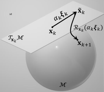
Figure 1: Retraction on the unit sphere. From point $\tilde{\mathbf{x}}_{k}=\mathbf{x}_{k}+\alpha_{k}\boldsymbol{\xi}_{k}$, where $\alpha_{k}$ is a stepsize employed along direction $\boldsymbol{\xi}_{k}$, point $\mathbf{x}_{k+1}$ on the manifold is obtained by normalization, i.e., $\mathbf{x}_{k+1}=\mathcal{R}_{\mathbf{x}_{k}}\big{(}\alpha_{k}\boldsymbol{\xi}_{k}\big{)}=\frac{\mathbf{x}_{k}+\alpha_{k}\boldsymbol{\xi}_{k}}{\|\mathbf{x}_{k}+\alpha_{k}\boldsymbol{\xi}_{k}\|_{2}}$ [13].

II-C Riemannian Optimization Methods

In Riemannian optimization, similar to classical unconstrained optimization, a descent search direction on the tangent space, $\boldsymbol{\xi}\in\mathcal{T}_{\mathbf{x}}\mathcal{M}$, satisfies the following condition:

$$\langle\mathrm{grad}f(\mathbf{x}),\boldsymbol{\xi}\rangle<0.$$ (4)

Several first and second order algorithms including Gradient Descent, Newton’s and approximate Newton methods have been extended in [13] to the Riemannian optimization settings. Also, stepsize rules are directly applicable, e.g., the Armijo stepsize rule with scalars $\bar{\alpha}>0,\beta,\sigma\in(0,1)$, which, at iteration $k$, finds the smallest non-negative integer $m$, satisfying:

$$f(\mathbf{x}_{k})-f\big{(}\mathcal{R}_{\mathbf{x}_{k}}(\beta^{m}\bar{\alpha}\boldsymbol{\xi}_{k})\big{)}\geq-\sigma\langle\mathrm{grad}f(\mathbf{x}_{k}),\beta^{m}\bar{\alpha}\boldsymbol{\xi}_{k}\rangle.$$ (5)

In what follows, we provide a brief overview of Riemannian optimization methods.

II-C1 Riemannian Gradient Descent

Algorithm 1 reviews the Riemannian Gradient Descent (see [13, Algorithm 1]) using the Armijo stepsize rule. It is shown in [13, Thm. 4.3.1] that Algorithm 1 converges to a critical (stationary) point of $f$, with linear convergence rate [13, Thm. 4.5.6 and Def. 4.5.1].

Input: $\mathcal{M}$, $f:\mathcal{M}\mapsto\mathbb{R}$, $\mathcal{R}_{\mathbf{x}}:\mathcal{T}_{\mathbf{x}}\mathcal{M}\mapsto\mathcal{M}$, scalars $\bar{\alpha}>0,\beta,\sigma\in(0,1)$, and $\epsilon>0$ (small).

Output: Critical point $\mathbf{x}^{*}\in\mathcal{M}$ of $f:\mathcal{M}\mapsto\mathbb{R}$

Initialization: $k=0$, $\mathbf{x}_{0}\in\mathcal{M}$;

while $\|\mathrm{grad}f(\mathbf{x}_{k})\|_{2}>\epsilon$ do

       Find direction $\boldsymbol{\xi}_{k}\in\mathcal{T}_{\mathbf{x}_{k}}\mathcal{M}$ satisfying (4);

       $\mathbf{x}_{k+1}=\mathcal{R}_{\mathbf{x}_{k}}(\beta^{m}\bar{\alpha}\boldsymbol{\xi}_{k})$ satisfying Armijo rule (5);

       $k=k+1$;

      

end while

Algorithm 1 Riemannian Gradient Descent

II-C2 Riemannian Newton’s Method

Algorithm 2 reviews the Riemannian Newton’s method (see [13, Algorithm 5]). The direction $\boldsymbol{\xi}_{k}\in\mathcal{T}_{\mathbf{x}_{k}}\mathcal{M}$ is obtained by solving the Newton equation (6), where the Jacobian $\mathbf{J}(\mathbf{x}_{k}):=\mathrm{hess}f(\mathbf{x}_{k})$,

$$\mathbf{J}(\mathbf{x}_{k}){\xi}_{k}=\mathrm{hess}f(\mathbf{x}_{k})[\boldsymbol{\xi}_{k}]=-\mathrm{grad}f(\mathbf{x}_{k}).$$ (6)

It is, however, not guaranteed that $\boldsymbol{\xi}_{k}$ is a descent direction unless $\mathrm{hess}f(\mathbf{x}_{k})$ is positive definite. Although the Riemannian Newton’s method enjoys a local superlinear (at least quadratic) convergence rate [13, Thm. 6.3.2], it lacks global convergence, i.e., there exist initial points for which the method does not converge [13]. In addition, evaluating the Hessian and solving (6) may be computationally expensive.

Input: $\mathcal{M}$, $f:\mathcal{M}\mapsto\mathbb{R}$, $\mathcal{R}_{\mathbf{x}}:\mathcal{T}_{\mathbf{x}}\mathcal{M}\mapsto\mathcal{M}$, scalar $\epsilon>0$ (small).

Output: Critical point $\mathbf{x}^{*}\in\mathcal{M}$ of $f:\mathcal{M}\mapsto\mathbb{R}$

Initialization: $k=0$, $\mathbf{x}_{0}\in\mathcal{M}$;

while $\|\mathrm{grad}f(\mathbf{x}_{k})\|_{2}>\epsilon$ do

       Find direction $\boldsymbol{\xi}_{k}\in\mathcal{T}_{\mathbf{x}_{k}}\mathcal{M}$ satisfying (6);

       $\mathbf{x}_{k+1}=\mathcal{R}_{\mathbf{x}_{k}}(\boldsymbol{\xi}_{k})$;

       $k=k+1$;

      

end while

Algorithm 2 Riemannian Newton’s Method

II-C3 Riemannian Approximate Newton Methods

To overcome the drawbacks of Newton’s method, [13, Sec. 8.2] presents approximate Newton methods, which maintain local superlinear convergence (under certain conditions), while having stronger global convergence properties, and require lower computational effort. A class of approximate Newton methods approximates/modifies the Jacobian, so that (6) becomes:

$$\big{[}\mathbf{J}(\mathbf{x}_{k})+\mathbf{E}_{k}\big{]}\boldsymbol{\xi}_{k}=-\mathrm{grad}f(\mathbf{x}_{k}),$$ (7)

where $\mathbf{E}_{k}$ denotes the approximation error, which is assumed to have sufficiently small bounds (in order to preserve the superlinear convergence).

III LF as a Riemannian Optimization Problem

We consider a radial distribution network with node 0 representing the slack node, typically a distribution substation. We denote the set of nodes, excluding the slack node, with $\mathcal{J}=\{1,2,...,J\}$. Exploiting the radial topology, we denote the set of branches (i.e., lines) with $\mathcal{J}$, where branch $j$ has node $j$ as its downstream node, and we label its upstream node with $i$. The set of branches whose upstream node is $j$ is denoted by $\mathcal{J^{\prime}}(j)$. At node $j$, $v_{j}$ is the squared voltage magnitude, $p_{j}$ and $q_{j}$ the net real and reactive power injections, with negative values representing power consumption. The slack node voltage $v_{0}$ is typically assumed to be fixed. At branch $j$, $P_{j}$ and $Q_{j}$ are the real and reactive power flows at the sending (upstream) end $i$, respectively, $l_{j}$ is the squared current magnitude, $r_{j}$ and $x_{j}$ the series resistance and reactance, and $a_{j}$ the transformer tap ratio [44]. The total shunt admittance at node $j$ including the capacitance of the lines connected to node $j$ is denoted by $Y_{j}=G_{j}-\imath B_{j}$, where $\imath=\sqrt{-1}$.

In what follows, we present the BFM formulation (Subsection III-A), the LF problem reformulation as a Riemannian optimization problem and the Riemannian gradient and Hessian calculations (Subsection III-B), the proposed retractions (Subsection III-C), and initializations (Subsection III-D).

III-A BFM Formulation

The LF equations of a radial network, using the BFM [30], and accounting for shunt admittances and transformer tap ratios [44], are given by:

$$\sum_{j^{\prime}\in\mathcal{J^{\prime}}(j)}{P_{j^{\prime}}}-P_{j}+{a_{j}^{2}}r_{j}{l_{j}}+G_{j}v_{j}=p_{j},\ \ \ \forall j\in\mathcal{J},$$ (8)

$$\sum_{j^{\prime}\in\mathcal{J^{\prime}}(j)}{Q_{j^{\prime}}}-Q_{j}+{a_{j}^{2}}x_{j}{l_{j}}-B_{j}v_{j}=q_{j},\ \ \ \forall j\in\mathcal{J},$$ (9)

$$v_{j}=\frac{v_{i}}{a_{j}^{2}}-2(r_{j}P_{j}+x_{j}Q_{j})+{a_{j}^{2}}(r_{j}^{2}+x_{j}^{2}){l_{j}},\forall j\in\mathcal{J},$$ (10)

$$v_{i}l_{j}=P_{j}^{2}+Q_{j}^{2},\ \ \ \forall j\in\mathcal{J},$$ (11)

where (8) and (9) ensure real and reactive power balance, respectively, at node $j\in\mathcal{J}$, (10) defines the voltage drop across line $j$, and (11) describes the nonlinear relation between the current of line $j$, the real and reactive power flowing along line $j$ and the voltage at the upstream node $i$.

Assumption 1.

A feasible LF solution exists for the BFM described by (8)–(11).

Assumption 1 is a very mild assumption, which generally holds for practical problems. Problematic cases are discussed in our prior work [10], which provides the means to diagnose them. On the other hand, the BFM may generally admit multiple solutions, however, in practical networks [45], with realistic resistance/reactance values and close to nominal substation voltage levels, the solution with practical voltage values is unique. Notably, equations (8)–(10) are linear, whereas (11) represents the surface of a second order cone for each line $j\in\mathcal{J}$. Relaxing (11) to an inequality in the context of an optimization problem yields the aforementioned SOCP relaxation [31], whose solution, however, is not always guaranteed to be result in a binding inequality [32]-[38] and hence not satisfy (11).

III-B Riemannian Optimization Problem Formulations

In this subsection, we present two Riemannian optimization formulations for the LF problem, considering: (i) a manifold represented by the full set of the LF equations (8)–(11), referred to as the BFM manifold, and (ii) a manifold corresponding to (11), referred to as the Quadratic Equality (QE) manifold.

III-B1 BFM Manifold

Consider the BFM, where we treat the real and reactive power injections, $p_{j}$ and $q_{j}$, as variables, and we add the following set of equations:

$$p_{j}=\bar{p}_{j},\qquad q_{j}=\bar{q}_{j},\qquad\forall j\in\mathcal{J},\\$$ (12)

with parameters $\bar{p}_{j}$ and $\bar{q}_{j}$ representing the values of the known injections. Let $\mathbf{x}$ be the vector of variables, with $\mathbf{x}=\begin{pmatrix}\mathbf{u}^{T}\quad\mathbf{w}^{T}\end{pmatrix}^{T}$, and vectors $\mathbf{u}$ and $\mathbf{w}$ given by $\mathbf{u}=\begin{pmatrix}\mathbf{P}^{T}\,\,\mathbf{Q}^{T}\,\,\mathbf{l}^{T}\,\,\mathbf{v}^{T}\end{pmatrix}^{T}$, and $\mathbf{w}=\begin{pmatrix}\mathbf{p}^{T}\,\,\mathbf{q}^{T}\end{pmatrix}^{T}$, respectively, where $\mathbf{P}$, $\mathbf{Q}$, $\mathbf{l}$, $\mathbf{v}$, $\mathbf{p}$, and $\mathbf{q}$, are the vectors of variables $P_{j}$, $Q_{j}$, $l_{j}$, $v_{j}$, $p_{j}$, and $q_{j}$ respectively. We define the BFM manifold as:

$$\mathcal{M}_{\textrm{BFM}}=\{\mathbf{x}\in\mathbb{R}^{6J}|\mathbf{F}_{\textrm{BFM}}(\mathbf{x})=\mathbf{0}\},$$ (13)

where $\mathbf{F}_{\textrm{BFM}}(\mathbf{x})=\mathbf{0}$ is the compact form of (8)-(11). Naturally, the LF solution will be obtained when the values of variables $p_{j}$ and $q_{j}$ are equal to the values of the known injections, i.e., when (12) holds. Hence, the basic idea is to define an optimization problem, which penalizes the mismatches in (12), while ensuring that variables $\mathbf{x}$ remain on the BFM manifold. This yields the following Riemannian optimization problem:

$$\min_{\mathbf{x}\in\mathcal{M}_{\textrm{BFM}}}f_{\textrm{BFM}}(\mathbf{x})={\|\mathbf{w}-\mathbf{\bar{w}}\|}_{2}^{2},$$ (14)

where $\mathbf{\bar{w}}=\begin{pmatrix}\mathbf{\bar{p}}^{T}\,\,\mathbf{\bar{q}}^{T}\end{pmatrix}^{T}$, is the vector of the known real and reactive power injections. Given Assumption 1, the optimal solution of problem (14) should be zero. Denote by $\mathbf{x}_{k}$ the vector obtained at the $k$-th iteration. Using (2), the Riemannian gradient associated with (14) becomes:

$$\textrm{grad}f_{\textrm{BFM}}(\mathbf{x}_{k})=2\mathbf{\Pi}_{\mathbf{x}_{k}}\begin{pmatrix}\mathbf{0}_{4J\times 1}\\ \mathbf{w}_{k}-\mathbf{\bar{w}}\end{pmatrix}.$$ (15)

Using (3) and the product rule for derivatives, the Riemannian Hessian is given by:

hess $$f_{\textrm{BFM}}(\mathbf{x}_{k})[\boldsymbol{\xi}_{k}]=\mathbf{\Pi}_{\mathbf{x}_{k}}\textrm{Dgrad}f_{\textrm{BFM}}(\mathbf{x}_{k})[\boldsymbol{\xi}_{k}],$$

$$=\mathbf{\Pi}_{\mathbf{x}_{k}}\left[2\mathbf{\Pi}_{\mathbf{x}_{k}}\begin{pmatrix}\mathbf{0}_{4J\times 4J}\quad\mathbf{0}_{4J\times 2J}\\ \mathbf{0}_{2J\times 4J}\quad\mathbf{I}_{2J\times 2J}\\ \end{pmatrix}+\mathbf{C}_{\mathbf{x}_{k}}\right]\boldsymbol{\xi}_{k},$$ (16)

for all $\boldsymbol{\xi}_{k}\in\mathcal{T}_{\mathbf{x}_{k}}\mathcal{M}_{\textrm{BFM}}$, where $\mathbf{C}_{\mathbf{x}_{k}}$ is a matrix involving the derivatives of $\mathbf{\Pi}_{\mathbf{x}}$ at $\mathbf{x}=\mathbf{x}_{k}$. It can be shown that the $n$-th column of $\mathbf{C}_{\mathbf{x}_{k}}$, denoted by $\mathbf{C}_{n,\mathbf{x}_{k}}$, equals:

$$\mathbf{C}_{n,\mathbf{x}_{k}}=2\boldsymbol{\Gamma}_{n,\mathbf{x}_{k}}^{T}\begin{pmatrix}\mathbf{0}_{4J\times 1}\\ \mathbf{w}_{k}-\mathbf{\bar{w}}\end{pmatrix},$$ (17)

where $\boldsymbol{\Gamma}_{n,\mathbf{x}_{k}}$ denotes the matrix to scalar derivative of $\mathbf{\Pi}_{\mathbf{x}}$ w.r.t. the $n$-th element of $\mathbf{x}$ at $\mathbf{x}=\mathbf{x}_{k}$.

III-B2 QE Manifold

Although the BFM manifold is a natural way to define the entire PF manifold in radial networks, inspired by the SOCP relaxation, we observe that (11) can be written by completing the squares so as to resemble the equation of a sphere. Hence, we define the QE manifold as follows:

$$\mathcal{M}_{\textrm{QE}}=\{\mathbf{u}\in\mathbb{R}^{4J}|\mathbf{F}_{\textrm{QE}}(\mathbf{u})=\mathbf{0}\},$$ (18)

where $\mathbf{F}_{\textrm{QE}}(\mathbf{u})=0$ is the compact form of (11), and $\mathbf{u}$ is the vector defined above including variables $P_{j}$, $Q_{j}$, $l_{j}$, and $v_{j}$. Notably, the QE manifold relies on vector $\mathbf{u}$ rather than the larger vector $\mathbf{x}$, because the real and reactive power injections, $\mathbf{p}$ and $\mathbf{q}$, respectively, are now considered parameters (instead of variables). Then, considering the QE manifold, the LF solution requires that equations (8)–(10) are satisfied. Representing (8)–(10) in a compact form as $\mathbf{Au}=\mathbf{b}$, where $\mathbf{A}$ is a $3J\times 4J$ matrix, and $\mathbf{b}$ a $3J\times 1$ vector that includes parameters $\mathbf{p}$ and $\mathbf{q}$, we define the following Riemannian optimization problem:

$$\min_{\mathbf{u}\in\mathcal{M}_{\textrm{QE}}}f_{\textrm{QE}}(\mathbf{u})=\|\mathbf{Au}-\mathbf{b}\|_{2}^{2},$$ (19)

whose objective function penalizes the mismatches in (8)–(10). Similarly to (14), given Assumption 1, the optimal solution of (19) should be zero. The Riemannian gradient and Hessian associated with (19) are now given by:

$$\textrm{grad}f_{\textrm{QE}}(\mathbf{u}_{k}) =2\mathbf{\Pi}_{\mathbf{u}_{k}}\mathbf{A}^{T}(\mathbf{Au}_{k}-\mathbf{b}),$$ (20)

$$\textrm{hess}f_{\textrm{QE}}(\mathbf{u}_{k})[\boldsymbol{\zeta}_{k}] =\mathbf{\Pi}_{\mathbf{u}_{k}}\textrm{Dgrad}f_{\textrm{QE}}(\mathbf{u}_{k})[\boldsymbol{\zeta}_{k}],$$

$$=\mathbf{\Pi}_{\mathbf{u}_{k}}\big{(}2\mathbf{\Pi}_{\mathbf{u}_{k}}\mathbf{A}^{T}\mathbf{A}+\mathbf{{L}}_{\mathbf{u}_{k}}\big{)}\boldsymbol{\zeta}_{k},$$ (21)

where vector $\boldsymbol{\zeta}_{k}\in\mathbb{R}^{4J}$ is used instead of $\boldsymbol{\xi}_{k}\in\mathbb{R}^{6J}$ to avoid confusion (since we use variables $\mathbf{u}$ instead of $\mathbf{x}$), and $\mathbf{{L}}_{\mathbf{u}_{k}}$ is a matrix involving the derivative of $\mathbf{\Pi}_{\mathbf{u}}$ at $\mathbf{u}=\mathbf{u}_{k}$, whose $n$-th column, denoted by $\mathbf{{L}}_{n,\mathbf{u}_{k}}$, is expressed as:

$$\mathbf{{L}}_{n,\mathbf{u}_{k}}=2\boldsymbol{\Lambda}_{n,\mathbf{u}_{k}}^{T}\mathbf{A}^{T}(\mathbf{A}\mathbf{u}_{k}-\mathbf{b}),$$ (22)

where $\boldsymbol{\Lambda}_{n,\mathbf{u}_{k}}$ denotes the matrix to scalar derivative of $\mathbf{\Pi}_{\mathbf{u}}$ w.r.t. the $n$-th element of $\mathbf{u}$ at $\mathbf{u}=\mathbf{u}_{k}$.

III-C Proposed Retractions

In this subsection, we propose retraction methods that map a tangent vector to the BFM and the QE manifolds. Recall that at the $k$-th iteration, using vector $\boldsymbol{\xi}_{k}$ without loss of generality, the retraction maps a point from the tangent space $\mathcal{T}_{\mathbf{x}_{k}}\mathcal{M}$, denoted by $\tilde{\mathbf{x}}_{k}=\mathbf{x}_{k}+\alpha_{k}\boldsymbol{\xi}_{k}$, where $\alpha_{k}$ is the stepsize and $\boldsymbol{\xi}_{k}$ the search direction, to the manifold $\mathcal{M}$, to obtain the next point denoted by $\mathbf{x}_{k+1}=\mathcal{R}_{\mathbf{x}_{k}}(\alpha_{k}\boldsymbol{\xi}_{k})$. In what follows, we consider the variables associated with a single line, say line $j$. To temporarily simplify notation, we drop the line subscripts of variables $P_{j}$, $Q_{j}$, and $l_{j}$ in (8)-(11), and we only show the iteration counter, i.e., $P_{k}$, $Q_{k}$, and $l_{k}$ for the $k$-th iteration.

III-C1 BFM Manifold Retraction

By analogy to the Backward-Forward Sweep variant in [46], retraction $\mathcal{R}^{\textsc{BFM}}$, involves a current update step followed by a voltage update step in a forward sweep manner starting from the root node, namely:

$$\underline{\mathcal{R}^{\textsc{BFM}}}:\quad P_{k+1}=\tilde{P}_{k},\quad Q_{k+1}=\tilde{Q}_{k},\quad l_{k+1}=\frac{\tilde{P}_{k}^{2}+\tilde{Q}_{k}^{2}}{{v}_{i,k+1}},\quad$$

$$v_{j,k+1}=\frac{{v}_{i,k+1}}{a_{j}^{2}}-2(r\tilde{P}_{k}+x\tilde{Q}_{k})+a_{j}^{2}(r^{2}+x^{2}){l}_{k+1},$$ (23)

with $\tilde{P}_{k}$, $\tilde{Q}_{k}$, $\tilde{l}_{k}$, $\tilde{v}_{k}$ denoting the values on the tangent space. The retracted values for $p_{k+1}$ and $q_{k+1}$ are obtained by solving for the rhs of (8) and (9), respectively, using the retracted values $P_{k+1}$, $Q_{k+1}$, $l_{k+1}$, and $v_{j,k+1}$ obtained in (23).

Lemma 1.

$\mathcal{R}^{\textsc{BFM}}$ satisfies the conditions of Definition 3.

The proof is included in the Appendix (Section -A).

III-C2 QE Manifold Retractions

We present two retractions that are inspired in part by the retraction on the unit sphere (Fig. 1) and the BFM geometry. Inspired by the SOCP representation of [31], rearranging the completed square terms in (18), we get $4{P_{k}}^{2}+4{Q_{k}}^{2}+({v_{i,k}}-{l_{k}})^{2}=({v_{i,k}}+{l_{k}})^{2}$, yielding:

$$\Big{(}\frac{2{P_{k}}}{{v_{i,k}}+{l_{k}}}\Big{)}^{2}+\Big{(}\frac{2{Q_{k}}}{{v_{i,k}}+{l_{k}}}\Big{)}^{2}+\Big{(}\frac{{v_{i,k}}-{l_{k}}}{{v_{i,k}}+{l_{k}}}\Big{)}^{2}=1.$$ (24)

Notably, (24) represents a sphere in $\mathbb{R}^{3}$ enabling retraction by normalization [13]. Retraction $\mathcal{R}^{\textsc{QE}}_{1}$ uses an identity mapping for $\tilde{v}_{j,k}$ and normalizes each term in parentheses in (24), which after some algebra yields:

$$\underline{\mathcal{R}^{\textsc{QE}}_{1}}:\qquad v_{j,k+1}=\tilde{v}_{j,k},\quad l_{k+1}=\frac{D_{k}+\tilde{l}_{k}-\tilde{v}_{i,k}}{D_{k}-\tilde{l}_{k}+\tilde{v}_{i,k}}\tilde{v}_{i,k},\qquad\qquad$$

$$P_{k+1}=\frac{2\tilde{P}_{k}\tilde{v}_{i,k}}{D_{k}-\tilde{l}_{k}+\tilde{v}_{i,k}},\quad Q_{k+1}=\frac{2\tilde{Q}_{k}\tilde{v}_{i,k}}{D_{k}-\tilde{l}_{k}+\tilde{v}_{i,k}},$$ (25)

where $D_{k}=\sqrt{4(\tilde{P}_{k})^{2}+4(\tilde{Q}_{k})^{2}+(\tilde{l}_{k}-\tilde{v}_{i,k})^{2}}$.

Lemma 2.

$\mathcal{R}^{\textsc{QE}}_{1}$ satisfies the conditions of Definition 3.

The proof is included in the Appendix (Section -B).

Retraction $\mathcal{R}^{\textsc{QE}}_{2}$ uses identity mappings for $\tilde{v}_{j,k}$, $\tilde{P}_{k}$, and $\tilde{Q}_{k}$ and updates the value of $l_{k+1}$ satisfying (18); it is given by:

$$\underline{\mathcal{R}^{\textsc{QE}}_{2}}:\qquad\qquad v_{j,k+1}=\tilde{v}_{j,k},\quad l_{k+1}=\frac{\tilde{P}_{k}^{2}+\tilde{Q}_{k}^{2}}{\tilde{v}_{i,k}},\qquad\quad\qquad$$

$$P_{k+1}=\tilde{P}_{k},\quad Q_{k+1}=\tilde{Q}_{k}.$$ (26)

Lemma 3.

$\mathcal{R}^{\textsc{QE}}_{2}$ satisfies the conditions of Definition 3.

The proof is included in the Appendix (Section -C).

III-D Proposed Initializations

The two proposed initializations are:

Flat: Flat start initialization in traditional LF methods (e.g., Newton-Raphson) sets $v_{j}$ equal to the substation voltage, and $l_{j}$, $P_{j}$ and $Q_{j}$ equal to zero.

Warm: Warm start initialization solves the LinDistFlow equations [39, 40]:

$$\sum_{j^{\prime}\in\mathcal{J^{\prime}}(j)}{P_{j^{\prime}}}-P_{j}+G_{j}v_{j}=p_{j},\ \ \ \forall j\in\mathcal{J},$$ (27)

$$\sum_{j^{\prime}\in\mathcal{J^{\prime}}(j)}{Q_{j^{\prime}}}-Q_{j}-B_{j}v_{j}=q_{j},\ \ \ \forall j\in\mathcal{J},$$ (28)

$$v_{j}-\frac{v_{i}}{a_{j}^{2}}+2(r_{j}P_{j}+x_{j}Q_{j})=0,\forall j\in\mathcal{J},$$ (29)

i.e., it solves (8)–(10), assuming zero currents, to obtain the initial values for $v_{j}$, $P_{j}$ and $Q_{j}$.

For both Flat and Warm, the initial points, $\mathbf{x}_{0}$ and $\mathbf{u}_{0}$, for the BFM and QE manifolds, are obtained by applying retractions $\mathcal{R}^{\textsc{BFM}}$ and $\mathcal{R}^{\textsc{QE}}_{2}$, respectively.

IV Proposed Approximate Newton Method

In this section, we present the proposed LF solution method, which is shown to belong to the category of Riemannian approximate Newton methods, and its application to the BFM and QE manifolds. Without loss of generality, we present the method using the variables represented by vector $\mathbf{x}$, which refers to the BFM manifold, noting that vector $\mathbf{u}$, which refers to the QE manifold, is included in vector $\mathbf{x}$. Function $f(\mathbf{x})$ represents the mismatches during the optimization process.

Consider the $k$-th iteration, at which we are found at point $\mathbf{x}_{k}$ (on the manifold), which does not attain the minimum of the Riemannian optimization problem, i.e., $f(\mathbf{x}_{k})$ is not zero; if it were, then we would have reached the LF solution, as $\mathbf{x}_{k}$ would be on the manifold and all equality constraints would be satisfied (zero mismatches). We aim at finding a descent direction $\boldsymbol{\xi}_{k}$ on the tangent space $\mathcal{T}_{\mathbf{x}_{k}}\mathcal{M}$, to move from point $\mathbf{x}_{k}$ to point $\tilde{\mathbf{x}}_{k}$, and then apply a retraction. Instead of employing the Riemannian gradient, as in Algorithm 1, we obtain direction $\boldsymbol{\xi}_{k}$, so that the new point $\tilde{\mathbf{x}}_{k}=\mathbf{x}_{k}+\boldsymbol{\xi}_{k}$ (assuming a stepsize equal to 1), which lies on the tangent space, ${\boldsymbol{\xi}_{k}\in\mathcal{T}_{\mathbf{x}_{k}}\mathcal{M}}$, also minimizes the mismatches, i.e.,

$$f(\tilde{\mathbf{x}}_{k})=f(\mathbf{x}_{k}+\boldsymbol{\xi}_{k})=0$$ (30)

The LF solution algorithm employing the proposed approximate Newton method is presented in Algorithm 3.

Input: $\mathcal{M}$, $f:\mathcal{M}\mapsto\mathbb{R}$, $\mathcal{R}_{\mathbf{x}}:\mathcal{T}_{\mathbf{x}}\mathcal{M}\mapsto\mathcal{M}$, scalars $\bar{\alpha}>0,\beta,\sigma\in(0,1)$, and $\epsilon>0$ (small).

Output: A critical point $\mathbf{x}^{*}\in\mathcal{M}$ of $f:\mathcal{M}\mapsto\mathbb{R}$

Initialization: $k=0$ and $\mathbf{x}_{0}\in\mathcal{M}$ ;

while $\|\mathrm{grad}f(\mathbf{x}_{k})\|_{2}>\epsilon$ do

       Find direction $\boldsymbol{\xi}_{k}\in\mathcal{T}_{\mathbf{x}_{k}}\mathcal{M}$ satisfying (30);

       $\mathbf{x}_{k+1}=\mathcal{R}_{\mathbf{x}_{k}}(\beta^{m}\bar{\alpha}\boldsymbol{\xi}_{k})$ satisfying Armijo rule (5);

       $k=k+1$;

      

end while

Algorithm 3 Proposed Approximate Newton Method

In what follows, we exemplify the algorithm on the BFM and the QE manifold.

IV-A Application to the BFM Manifold

Employing the BFM manifold, we obtain direction $\boldsymbol{\xi}_{k}=(\boldsymbol{\zeta}_{k}^{T}\ \boldsymbol{\eta}^{T}_{k})^{T}$, where $\boldsymbol{\zeta}$ and $\boldsymbol{\eta}$ are search directions along u and w variables, respectively, by solving the following system of linear equations (with variables $\boldsymbol{\xi}_{k}$):

$$\boldsymbol{\xi}_{k}\in\mathcal{T}_{\mathbf{x}_{k}}\mathcal{M}_{\textrm{BFM}},\qquad\mathbf{w}_{k}+\boldsymbol{\eta}_{k}=\mathbf{\bar{w}},$$ (31)

where the first set represents equations (8)–(10) with variables $\boldsymbol{\xi}_{k}$ (instead of $\mathbf{x}_{k}$) and a linear approximation of (11) —which is presented in (35) in the Appendix— and the second set of equations is directly obtained by applying (30) to $f_{\textrm{BFM}}(\mathbf{x}_{k}+\mathbf{\boldsymbol{\xi}_{k}})=\|\mathbf{w}_{k}+\boldsymbol{\eta}_{k}-\mathbf{\bar{w}}\|_{2}^{2}$ given by (14). Hence, one can think of the solution of (31), assuming linearly independent rows, as the solution of minimizing $f_{\textrm{BFM}}$ over the tangent space around $\mathbf{x}_{k}$, expressed as $\min_{\boldsymbol{\xi}_{k}\in\mathcal{T}_{\mathbf{x}_{k}}\mathcal{M}_{\textrm{BFM}}}f_{\textrm{BFM}}(\mathbf{x}_{k}+\mathbf{\boldsymbol{\xi}_{k}})$, where the decision variables are $\boldsymbol{\xi}_{k}$.

The following proposition summarizes the properties of the proposed LF solution method applied to the BFM manifold.

Proposition 1.

Algorithm 3, applied to the BFM manifold, is a Riemannian approximate Newton method, with guaranteed descent and local superlinear convergence rate.

The proof is included in the Appendix (Section -D).

IV-B Application to the QE manifold

Similarly to (31), we obtain direction $\boldsymbol{\zeta}_{k}$ by solving the following system of linear equations:

$$\boldsymbol{\zeta}_{k}\in\mathcal{T}_{\mathbf{u}_{k}}\mathcal{M}_{\textrm{QE}},\qquad\mathbf{A}(\mathbf{u}_{k}+\boldsymbol{\zeta}_{k})=\mathbf{b},$$ (32)

where the second set of equations is directly obtained by applying (30) to $f_{\textrm{QE}}(\mathbf{u}_{k}+\mathbf{\boldsymbol{\zeta}_{k}})=\|\mathbf{A}(\mathbf{u}_{k}+\boldsymbol{\zeta}_{k})-\mathbf{b}\|_{2}^{2}$ given by (19). The solution of (32), assuming linearly independent rows, can be viewed as the solution of minimizing $f_{\textrm{QE}}$ over the tangent space around $\mathbf{u}_{k}$, expressed as $\min_{\boldsymbol{\zeta}_{k}\in\mathcal{T}_{\mathbf{u}_{k}}\mathcal{M}_{\textrm{QE}}}f_{\textrm{QE}}(\mathbf{u}_{k}+\mathbf{\boldsymbol{\zeta}_{k}})$, where the decision variables are $\boldsymbol{\zeta}_{k}$. The following proposition essentially states that the properties of Proposition 1 carry over to the QE manifold.

Proposition 2.

Algorithm 3, applied to the QE manifold, is a Riemannian approximate Newton method, with guaranteed descent and local superlinear convergence rate.

The proof is included in the Appendix (Section -E).

Although the proposed method is an exact LF solution method, executing it only for one iteration yields an approximate LF solution. In fact, as we will show later, the numerical comparisons illustrate that the first iteration employing Warm and $\mathcal{R}^{\textsc{QE}}_{2}$ yields a higher quality LF solution compared with both LinDistFlow and the linear approximant proposed in [27]. Lastly, the following Corollary relates the two initializations (Flat and Warm) when combined with retraction $\mathcal{R}^{\textsc{QE}}_{2}$.

Corollary 1.

The first iteration of Algorithm 3, employing $\mathcal{R}^{\textsc{QE}}_{2}$ and Flat, yields the Warm initial point.

The proof is included in the Appendix (Section -F).

V Numerical Comparisons

In this section, we evaluate the performance of the Riemannian optimization methods —namely the Riemannian Gradient Descent, the Riemannian Newton’s and the proposed Riemannian approximate Newton methods— on several standard IEEE radial distribution test networks with $18$, $22$, $33$, $69$, $85$, and $141$ nodes [47], as well as on single-phase equivalents of the IEEE-$13$, IEEE-$37$, and IEEE-$123$ test networks [48]. We refer to the test networks as 13-node, 18-node, etc. All methods are implemented in Matlab R2018a and tested on a desktop Intel i5-2500 at 3.3 GHz with 8 GB RAM. We added an additional stopping criterion in all Algorithms requiring the maximum voltage change in consecutive iterations be less than a small tolerance ($\delta>0$), modifying the while-loop as follows:

$$\textbf{while }\|\mathrm{grad}f(\mathbf{x}_{k})\|_{2}>\epsilon\text{ or }\|\sqrt{\mathbf{v}_{k+1}}-\sqrt{\mathbf{v}_{k}}\|_{\infty}>\ \delta,$$

which better fits the LF problem and ensures a consistent comparison with the Newton-Raphson method. The tolerances are $\epsilon=\delta=10^{-6}$. Armijo parameters are set to $\beta=0.3$, $\sigma=0.05$ for all methods, $\bar{\alpha}=4.5$ for Riemannian Gradient on the BFM manifold, and $\bar{\alpha}=1$ for the other methods. Computation times are reported in milliseconds (ms) and are obtained after running the main loop for $100$K times; they do not include pre-processing or the initialization.

The remainder of this section is structured as follows. In Subsection V-A, we compare the performance of the Riemannian optimization methods for the Base Case, which employs Warm initialization, and, for the QE manifold, retraction $\mathcal{R}^{\textsc{QE}}_{2}$. In Subsection V-B, we evaluate the impact of Flat and $\mathcal{R}^{\textsc{QE}}_{1}$, as an alternative initialization and retraction, respectively. In Subsection V-C, we compare the proposed method with the traditional Newton-Raphson method, considering, in addition, increased loading conditions and larger test networks. In Subsection V-D, we consider the first iteration of the proposed method as a linear approximant to the LF problem, and we compare its accuracy with existing approximate LF solution methods (LinDistFlow and [27]). Lastly, in Subsection V-E, we illustrate similarities and differences with the well-known Backward-Forward Sweep method.

V-A Base Case Comparison

TABLE I: Performance of Riemannian Optimization Methods (Base Case)

Network	Time (ms)	Riemannian Optimization Methods
	Iterations	GD(BFM)	P(BFM)	GD(QE)	N(QE)	P(QE)
13-node	Time	0.13$\times 10^{3}$	1.39	0.32$\times 10^{3}$	0.77	0.49
	Iter #	162	3	1,420	3	3
18-node	Time	21.6$\times 10^{3}$	1.89	93$\times 10^{3}$	2.7	0.55
	Iter #	22,221	3	438,042	5	3
22-node	Time	0.18$\times 10^{3}$	1.51	0.33$\times 10^{3}$	1.57	0.48
	Iter #	151	2	1,288	3	2
33-node	Time	3.8$\times 10^{3}$	3.36	54.2$\times 10^{3}$	3.54	0.96
	Iter #	2,201	3	186,731	3	3
37-node	Time	0.72$\times 10^{3}$	2.97	105.6$\times 10^{3}$	24.3	0.72
	Iter #	363	2	213,478	3	2
69-node	Time	4.38$\times 10^{3}$	7.17	3.5$\times 10^{3}$	14.3	1.98
	Iter #	1,232	3	9,094	3	3
85-node	Time	19.2$\times 10^{3}$	8.61	14.6$\times 10^{3}$	37.1	2.34
	Iter #	4,383	3	31,415	4	3
123-node	Time	23.5$\times 10^{3}$	14.83	35.7$\times 10^{3}$	125.7	3.29
	Iter #	3,622	3	46,145	4	3
141-node	Time	69.3$\times 10^{3}$	14.29	47.5$\times 10^{3}$	140	3.75
	Iter #	9,709	3	64,469	4	3

In Table I, we compare the performance of the Riemannian optimization methods, for the Base Case, in terms of computation time and iterations. The methods are denoted by: “GD” for Gradient Descent; “N” for Newton’s; “P” for the proposed approximate Newton method; in parentheses we show the applicable manifold, BFM or QE. We note that the times reported for Newton’s method do not include the Hessian evaluation step, which was a time-consuming task that renders the performance of this method not acceptable in practice; for this reason we only included the results for the QE manifold mainly to compare the iterations it takes to converge with the proposed approximate Newton method.

The results show that the Riemannian GD converges after a considerably large number of iterations and requires significant computation time (in the order of seconds). Conversely, the Riemannian Newton’s method and the proposed approximate Newton method converge after only a few iterations (as expected), with the proposed method outperforming Newton’s method in terms of computational effort in all test networks. The results indicate that Newton’s method (even excluding the Hessian evaluation) is slower than the proposed method by a factor that ranges from about 1.5 for the $13$-node to about 38 for the $123$-node test network. In addition, we note that GD(BFM) takes much less iterations to converge, but each iteration is slower compared to GD(QE), by a factor ranging from 3.5 to 9.7, mainly due to the computational effort it takes to execute the retraction $\mathcal{R}^{\textsc{BFM}}$ compared to $\mathcal{R}^{\textsc{QE}}_{2}$. For the same reason, although the P(BFM) and P(QE) converge at the same number of iterations, the former is slower by a factor ranging from 2.8 to 4.5.

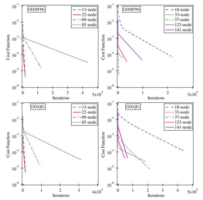
Figure 2: Trajectories (cost function value vs. iterations); Top: GD(BFM); Bottom: GD(QE). The vertical axis is in logarithmic scale.

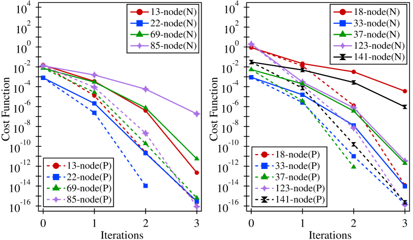
Figure 3: Trajectories (cost function value vs. iterations); N(QE): solid lines; P(QE): dashed lines. The vertical axis is in logarithmic scale.

Figure 2 illustrates the cost function trajectories for GD(BFM) (top) and GD(QE) (bottom), for all test networks. We observe that the cost function of GD on the BFM (QE) manifold decreases over consecutive iterations, and reaches a value of $10^{-4}$ within around 80 (760), 20K (455K), 20 (320), 420 (53K), 100 (91K), 700 (5.7K), 3K (22K), 2K (30K), and 7.7K (52K) iterations for the $13\text{-},$ $18\text{-},$ $22\text{-},$ $33\text{-},$ $37\text{-},$ $69\text{-},$ $85\text{-},$ $123\text{-},$ and $141\text{-}$node test networks, respectively.

Figure 3 shows the cost function trajectories of the N(QE) and P(QE) for up to 3 iterations (since the latter method converges in at most 3 iterations for the employed test networks). Notably, P(QE) curves are always below the corresponding N(QE) curves for all networks. In most cases, the difference in terms of cost improvement in the first iteration is about one order of magnitude. Also, note that whereas, for instance, the cost function of the $13$-node and $69$-node test networks is reduced to at least $0.01$ of its initial value in one or two iterations in Fig. 3, GD(QE) —see Fig. 2— requires 653 and 6,260 iterations, respectively, to reach the same reduction.

V-B Comparison of Alternative Initializations and Retractions

TABLE II: Performance of Flat on Riemannian Newton’s and Proposed Approximate Newton Methods (Comparison with Warm)

Network	Time (ms)	Riemannian Optimization Methods
	Iterations	P(BFM)	N(QE)	P(QE)
$13$-node	Time	2.21 (+0.82)	1.26 (+0.49)	0.61 (+0.12)
	Iter #	4 (+1)	5 (+2)	4 (+1)
$18$-node	Time	3.03 (+1.14)	3.77 (+1.07)	0.8 (+0.25)
	Iter #	4 (+1)	7 (+2)	4 (+1)
$22$-node	Time	2.63 (+1.12)	2.03 (+0.46)	0.55 (+0.07)
	Iter #	3 (+1)	4 (+1)	3 (+1)
$33$-node	Time	5.25 (+1.89)	6.3 (+2.76)	1.05 (+0.09)
	Iter #	4 (+1)	5 (+2)	4 (+1)
$37$-node	Time	4.4 (+1.43)	24.6 (+0.3)	0.82 (+0.1)
	Iter #	3 (+1)	5 (+2)	3 (+1)
$69$-node	Time	11 (+3.83)	27.7 (+13.4)	2.12 (+0.14)
	Iter #	4 (+1)	6 (+3)	4 (+1)
$85$-node	Time	13.49 (+4.88)	59.8 (+22.7)	2.49 (+0.15)
	Iter #	4 (+1)	6 (+1)	4 (+1)
$123$-node	Time	20.28 (+5.45)	153 (+27.3)	3.72 (+0.43)
	Iter #	4 (+1)	5 (+1)	4 (+1)
$141$-node	Time	22.39 (+8.1)	182.9 (+42.9)	3.96 (+0.21)
	Iter #	4 (+1)	5 (+1)	4 (+1)

In Table II, we evaluate the impact of Flat on the performance of Riemannian Newton’s method and the proposed approximate Newton method. The values in parentheses show the differences when Warm is employed, i.e., with the results of Table I. The comparison verifies that Flat, which is considerably further to the optimal solution compared with Warm, performs worse in terms of both computation times and iterations (all differences are positive). Notably, Corollary 1 implies that P(QE), employing Flat and $\mathcal{R}^{\textsc{QE}}_{2}$, requires one more iteration compared with employing Warm. The results in Table II verify this outcome; the difference in time is actually the time required to execute the first iteration, which is in general lower than the average time per P(QE) iteration in Table I. In addition, P(QE) is affected much less (the computation time increase ranges from 0.07 ms for the 22-node to 0.43 ms for the 123-node test network) compared with Newton’s method (whose computation time increase ranges from 0.46 ms to 27.3 ms for the same networks); hence, the differences observed in the Base Case (Table I) become larger when employing Flat. Newton’s method is slower than the proposed method by a factor that ranges from 2 for the 13-node to 41 for the 123-node test network. In general, the average time per iteration increases for P(BFM), which, compared with P(QE), becomes slower by a factor ranging from 3.6 to 5.6.

TABLE III: Performance of $\mathcal{R}^{\textsc{QE}}_{1}$ on Proposed Approximate Newton Method (Comparison with $\mathcal{R}^{\textsc{QE}}_{2}$).

Network	Time (ms)	Initializations
	Iterations	Flat	Warm
$13$-node	Time	0.73 (+0.12)	0.58 (+0.09)
	Iter #	4 (0)	3 (0)
$18$-node	Time	2.12 (+1.32)	0.64 (+0.09)
	Iter #	9 (+5)	3 (0)
$22$-node	Time	0.64 (+0.09)	0.54 (+0.06)
	Iter #	3 (0)	2 (0)
$33$-node	Time	1.17 (+0.12)	1.05 (+0.09)
	Iter #	4 (0)	3 (0)
$37$-node	Time	1.29 (+0.47)	0.79 (+0.07)
	Iter #	4 (+1)	2 (0)
$69$-node	Time	2.27 (+0.15)	2.09 (+0.11)
	Iter #	4 (0)	3 (0)
$85$-node	Time	2.61 (+0.12)	2.44 (+0.10)
	Iter #	4 (0)	3 (0)
$123$-node	Time	3.87 (+0.15)	3.42 (+0.13)
	Iter #	4 (0)	3 (0)
$141$-node	Time	5.45 (+1.49)	3.88 (+0.13)
	Iter #	5 (+1)	3 (0)

In Table III, we evaluate the impact of $\mathcal{R}^{\textsc{QE}}_{1}$ on the performance of the proposed approximate Newton method, which stands out as the most computationally efficient method, for both Flat and Warm. The values in parentheses show the differences when $\mathcal{R}^{\textsc{QE}}_{2}$ is employed with either Flat or Warm. The comparison suggests that when a closer initialization (Warm) is employed, both retractions perform well (yield the same number of iterations) with $\mathcal{R}^{\textsc{QE}}_{1}$ being slightly less computationally efficient —the computation time increase is up to 0.13 ms, ranging from 3% to 18%. The impact of $\mathcal{R}^{\textsc{QE}}_{1}$ combined with Flat is occasionally more severe (see, e.g., the 18-node test network, where the iterations increase by 5, and the computation time also increases by 165%).

Lastly, we experimented with initial points selected intentionally to differ substantially from a reasonable LF solution. Unreasonably low voltage and high current values were used. We tested all methods on the $13$-node test network and observed convergence to a solution with low voltages that are not met in practical networks. This was not a surprise. LF equations (8)–(11), in general, admit multiple solutions, however, the solution with practical voltage magnitudes — around 1 per-unit (p.u.) — is unique [45]. In fact, [45] shows a small example with two solutions; the realistic one and a low voltage one that is the type of solution we reached when we started from unreasonably low voltages.

V-C Comparison with the Newton-Raphson Method

In this subsection, we compare the proposed Riemannian approximate Newton method with the traditional Newton-Raphson (NR) method (MATPOWER’s implementation [47]).

In Table IV, we compare the performance of the NR method, using both Flat and Warm initializations, with P(QE). The values in parentheses show the differences; e.g., positive values in time suggest that NR is slower compared to P(QE). The voltage phase angles required to warm start NR were recovered using [31]. The results show the same number of iterations and similar computational effort, implying that the proposed Riemannian approximate Newton method can achieve comparable performance with the NR method.

TABLE IV: Performance of Newton-Raphson Method (Comparison with the Proposed P(QE) Method).

Network	Time (ms)	Initializations
	Iterations	Flat	Warm
$13$-node	Time	1.15 (+0.54)	0.90 (+0.41)
	Iter #	4 (0)	3 (0)
$18$-node	Time	1.23 (+0.43)	0.98 (+0.43)
	Iter #	4 (0)	3 (0)
$22$-node	Time	1.02 (+0.47)	0.70 (+0.22)
	Iter #	3 (0)	2 (0)
$33$-node	Time	1.54 (+0.49)	1.19 (+0.23)
	Iter #	4 (0)	3 (0)
$37$-node	Time	1.22 (+0.4)	0.79 (+0.07)
	Iter #	3 (0)	2 (0)
$69$-node	Time	2.30 (+0.18)	1.79 (-0.19)
	Iter #	4 (0)	3 (0)
$85$-node	Time	2.70 (+0.21)	2.12 (-0.23)
	Iter #	4 (0)	3 (0)
$123$-node	Time	3.45 (-0.27)	2.59 (-0.7)
	Iter #	4 (0)	3 (0)
$141$-node	Time	3.94 (-0.02)	2.99 (-0.75)
	Iter #	4 (0)	3 (0)

LF methods usually require more iterations and computational effort in higher loading conditions. In Table V, we compare NR with P(QE), using Warm and $\mathcal{R}^{\textsc{QE}}_{2}$, under two increased loading scenarios, namely a medium and a high loading scenario. Loading values are adjusted by a factor whose value is given in the first column of Table V for each network. The values in parentheses show the differences with P(QE) obtained under the same loading conditions. Positive (negative) differences declare worse (better) performance for NR compared with P(QE). Indeed, the results in Table V show that the computation time increases by up to 1 ms for the medium and by up to 2 ms for the high loading scenario for the NR method (comparing with the values for the base loading scenario in Table IV). P(QE) exhibits an increase up to 0.44 ms for the medium and up to 2.66 ms for the high loading scenario (comparing with the values for the base loading scenario in Table I). Overall, the results for both methods under increased loading scenarios are comparable; the iterations remain practically the same (occasionally NR may need one more iteration) and the times are still in the order of a few milliseconds. We also note that we tested P(BFM) with Warm initialization. In almost all networks, the number of iterations was the same, but each P(BFM) iteration was slower compared with the P(QE) by a factor that ranged from 3.1 to 4.6, for both the medium and high loading scenarios, indicating a similar behavior with the base loading (reported in Table I).

TABLE V: Performance of Newton-Raphson under Increased Loading Scenarios (Comparison with the Proposed P(QE) Method)

Network	Time (ms)	Loading Scenario
	Iterations	Medium	High
$13$-node	Time	1.21 (+0.51)	1.49 (+0.62)
M:$\times 2.5$; H:$\times 3.5$	Iter #	4 (0)	5 (0)
$18$-node	Time	0.99 (+0.34)	1.32 (+0.44)
M:$\times 1.5$; H:$\times 2$	Iter #	3 (0)	4 (0)
$22$-node	Time	1.38 (+0.64)	1.73 (+0.52)
M:$\times 7$; H:$\times 10$	Iter #	4 (+1)	5 (0)
$33$-node	Time	1.59 (+0.59)	1.99 (+0.34)
M:$\times 2.5$; H:$\times 3.5$	Iter #	4 (+1)	5 (0)
$37$-node	Time	1.19 (+0.11)	1.97 (+0.18)
M:$\times 5$; H:$\times 7.5$	Iter #	3 (0)	5 (0)
$69$-node	Time	1.78 (-0.27)	2.89 (-0.48)
M:$\times 2$; H:$\times 3$	Iter #	3 (0)	5 (0)
$85$-node	Time	2.08 (-0.32)	4.11 (+0.15)
M:$\times 1.5$; H:$\times 2.5$	Iter #	3 (0)	6 (+1)
$123$-node	Time	3.34 (+0.08)	5.04 (-0.35)
M:$\times 3$; H:$\times 4.5$	Iter #	4 (+1)	6 (+1)
$141$-node	Time	3.99 (+0.10)	4.97 (-1.44)
M:$\times 3$; H:$\times 4$	Iter #	4 (+1)	5 (0)

TABLE VI: Performance of Proposed P(QE) Method on Larger Networks (Newton-Raphson Performance in Parentheses).

Network	Time (ms)	Loading Scenario
	Iterations	Base	Medium	High
	[Load]	[$\times 1$]	[$\times 2.5$]	[$\times 3.2]$
$906$-node	Time	22.5 (17.2)	29.9 (23.2)	30.2 (28.8)
	Iter #	3 (3)	4 (4)	4 (5)
	[Load]	$[\times 1$]	$[\times 1.5$]	[$\times 1.9$]
$2500$-node	Time	72.4 (49.3)	96.7 (65.6)	121.0 (82.2)
	Iter #	3 (3)	4 (4)	5 (5)

We further elaborate on the performance under several loading conditions for larger networks, a $906$-node European low voltage test network [48], and a $2500$-node test network that is the single-phase equivalent of the $8500$-node network in [48]. The results for the P(QE) method are presented in Table VI; the values in parentheses are the respective NR results. Although NR seems to perform better, the results are in the same order of magnitude (tens of milliseconds), which further enhances the argument that the proposed method achieves comparable performance with NR. Lastly, we tested the performance of P(BFM). The results indicated the same number of iterations and an increase in computation times by a factor of 6 and 7.6, for the $906$-node and the $2500$-node networks, respectively, under all loading conditions.

V-D Comparison of Approximate LF Solutions

In this subsection, we consider approximate (not exact) LF solutions obtained by the first iteration of P(QE), employing Warm and $\mathcal{R}^{\textsc{QE}}_{2}$, referred to as the “proposed approximant.”

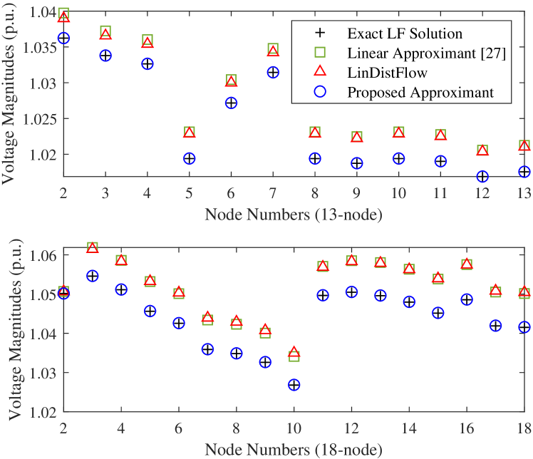
Figure 4: Comparison of approximate LF solutions on the $13$-node (upper) and the $18$-node (lower) test networks.

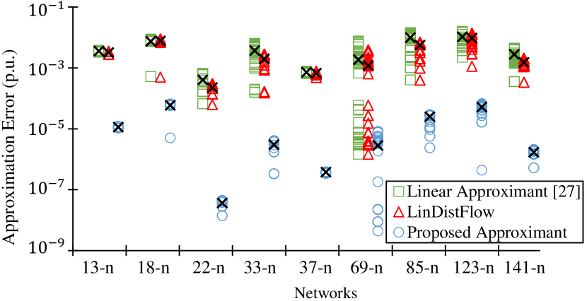
Figure 5: Voltage approximation error of the linear approximant in [27], the LinDistFlow solution and the proposed approximant. The “x” symbols represent the mean values. The vertical axis is in logarithmic scale.

Figure 4 illustrates the voltage magnitudes obtained by the linear approximant in [27], the LinDistFlow solution and the proposed approximant —including also the exact LF solution— for the 13-node and 18-node test networks. Note that, by definition of Warm, the LinDistFlow solution is the initial point of P(QE), hence, it is expected that the latter outperforms the former. Figure 5 illustrates the voltage approximation errors and their mean values for all methods. The proposed approximant outperforms other approximants by at least two orders of magnitude on all test networks. LinDistFlow achieves generally slightly better results compared with [27] (recall, however, that the latter applies to meshed networks as well), which verifies the remarks in [27] that LinDistFlow seems to improve the quality of their linear approximant (recall that the LinDistFlow solution is obtained by a non-linear change of coordinates in [27] and assuming zero shunt admittances); however, we observe that [27] yields a slightly better approximation than LinDistFlow in the 18-node test network.

V-E Comparison with the Backward-Forward Sweep Method

Last but not least, we consider the Backward-Forward Sweep (BFS) method, which has been proven to work well in radial networks. Among several BFS variants, we discuss the approach proposed in [46], as its forward sweep step (from the root to the leaf nodes) is identical to the $\mathcal{R}^{\textsc{BFM}}$ retraction. At the backward sweep step (from leaf nodes to the root), BFS first moves from $\mathbf{x}_{k}$ to $\tilde{\mathbf{x}}_{k}$; then, at the forward sweep step, it applies $\mathcal{R}^{\textsc{BFM}}$ to find point $\tilde{\mathbf{x}}_{k+1}$ (on the BFM manifold). The backward sweep step —which is described using the receiving-end power flows in [46]— can be equivalently written using the sending-end flows, as follows:

Backward Sweep Step: $\tilde{p}_{j,k}=\bar{p}_{j}$, $\tilde{q}_{j,k}=\bar{q}_{j}$, $\tilde{v}_{j,k}=v_{j,k}$,

$$\begin{split}\tilde{l}_{j,k}=\Big{[}&\big{(}\sum_{j^{\prime}\in\mathcal{J^{\prime}}(j)}{\tilde{P}_{j^{\prime},k}}+G_{j}\tilde{v}_{j,k}-\tilde{p}_{j}\big{)}^{2}\\ &+\big{(}\sum_{j^{\prime}\in\mathcal{J^{\prime}}(j)}{\tilde{Q}_{j^{\prime},k}}-B_{j}\tilde{v}_{j,k}-\tilde{q}_{j}\big{)}^{2}\Big{]}/\tilde{v}_{j,k},\end{split}$$

and then $\tilde{P}_{j,k}$ and $\tilde{Q}_{j,k}$ are obtained from (8) and (9) using $\tilde{P}_{j^{\prime},k},\tilde{v}_{j,k}$, $\tilde{l}_{j,k}$, and $\tilde{p}_{j,k}$, $\tilde{q}_{j,k}$. Note the similarity with the direction finding step of P(BFM), where we also require $\tilde{p}_{j,k}=\bar{p}_{j}$, and $\tilde{q}_{j,k}=\bar{q}_{j}$ —see the second set of $\mathbf{w}_{k}+\boldsymbol{\eta}_{k}=\mathbf{\bar{w}}$ part in (31). Hence, the difference between BFS and P(BFM) is in the direction $\boldsymbol{\xi}_{k}$. While both methods use the known nodal injections $\bar{p}_{j}$, and $\bar{q}_{j}$, BFS finds the direction by applying the backward sweep step, whereas P(BFM) requires the direction to be on the tangent space of the BFM manifold that is obtained by the solution of a linear system. In other words, BFS also stays on the BFM manifold at each iteration but moves in a different direction.

We ran BFS on all test networks, and even though it generally took the same or a few more iterations to reach the solution (within the same tolerances), it was up to one order of magnitude faster. Following our previous analysis, this result is not a surprise, as the P(BFM) requires the solution of a linear system in the direction finding step. Figure 6 illustrates the cost function trajectories of P(BFM) and the evaluation of this function for the BFS method. As expected, since the proposed method minimizes this function, P(BFM) trajectories are below the BFS ones; we also observe that BFS does not exhibit noticeable progress after the first and second iterations for the $37$-node and $123$-node test cases, respectively.

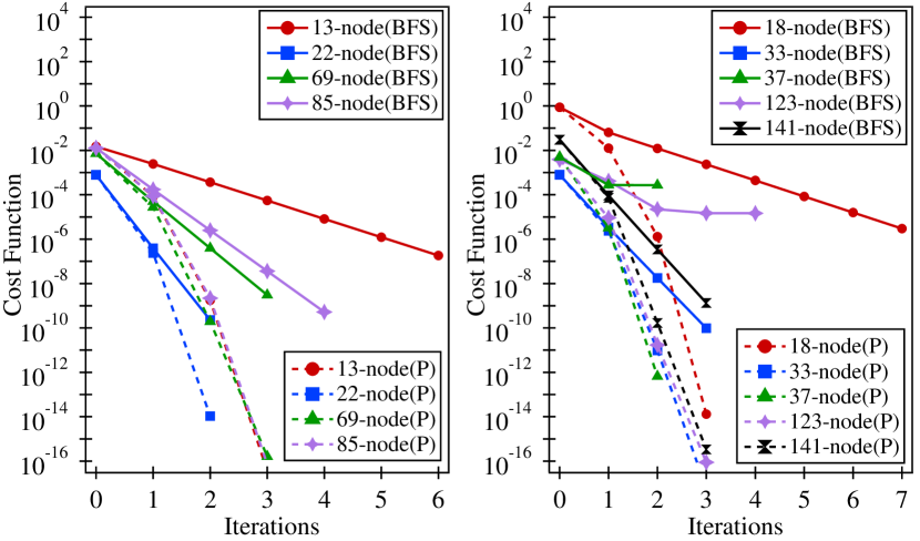
Figure 6: Trajectories (cost function value versus iterations); BFS: solid lines; P(BFM): dashed lines. The vertical axis is in logarithmic scale.

Lastly, we should mention that the performance of BFS does not undermine the value of the proposed method. The derived results and guarantees are promising for the application of Riemannian optimization to the more complicated OPF problem. Furthermore, it has been observed that BFS may diverge under a high constant impedance loading condition (e.g., [52] and [53] report such cases on another BFS variant). On an instance of the $123$-node test network (we replaced half of its constant power loads with their equivalent constant impedance, and applied a loading factor of 15.1), P(BFM) converged in 4 iterations with voltages spanning from about 0.7 to 1 p.u., whereas BFS exhibited oscillations in the voltage trajectory and diverged after 1K iterations.

VI Conclusions and Future Research

In this paper, we introduced a novel Riemannian optimization approach to the LF problem in radial distribution networks, employing the branch flow model. Our proposed method was shown to fall into the category of Riemannian approximate Newton methods, and guarantee descent at each iteration while maintaining a local superlinear convergence rate. Extensive numerical results illustrated that the proposed method outperforms other Riemannian optimization methods, namely the Riemannian Gradient Descent and the Riemannian Newton’s method, and that it achieves comparable performance with the traditional Newton-Raphson method. Also, we observed that the first iteration of the proposed method yields an approximate LF solution that is of higher quality (by at least two orders of magnitude) compared with other linear LF approximants. Lastly, we presented an interesting comparison with the well-known backward-forward sweep method, illustrating that while both methods essentially stay on the manifold, they move along different directions.

Our future research considers two directions. Firstly, we plan to extend the proposed Riemannian LF solution method to a general multi-phase power distribution network. In a multi-phase setting, the presence of mutual admittances between phases adds several degrees of complexity to the BFM and requires identifying new valid retractions. Secondly, and perhaps most importantly, we plan to address the more challenging OPF problem. In an OPF setting, the BFM manifold combined with operational constraints yields a non-smooth manifold that requires approaches such as the Riemannian augmented Lagrangian or exact penalty methods introduced in [54].

[Omitted Proofs]

-A Proof of Lemma 1

The proof for the centering condition is straightforward, since a zero tangent vector yields the tangent point, i.e., the current iterate $\mathbf{x}_{k}$. For the local rigidity condition, without loss of generality, we assume that the stepsize $\alpha_{k}$ is 1. We first consider the retraction associated with the variable $l_{k+1}$. Taking the derivative at $t=0$ yields:

$$\frac{\mathrm{d}}{\mathrm{d}t}\mathcal{R}^{\textsc{BFM}}_{\mathbf{x}_{k},l}(t\boldsymbol{\xi}_{k})|_{t=0}=\frac{2(\zeta_{k}^{P}P_{k}+\zeta_{k}^{Q}Q_{k})v_{i,k}-\zeta_{k}^{v}(P_{k}^{2}+Q_{k}^{2})}{v_{i,k}^{2}},$$ (33)

where $\zeta_{k}^{P},\zeta_{k}^{Q},\zeta_{k}^{v}$ denote the elements of $\boldsymbol{\xi}_{k}$ associated with $P_{k}$, $Q_{k}$, and $v_{i,k}$, respectively. Using the fact that $\mathbf{x}_{k}$ lies on the manifold, we have:

$$P_{k}^{2}+Q_{k}^{2}=l_{k}v_{i,k},$$ (34)

whose tangent space is characterized as:

$$2(\zeta_{k}^{P}P_{k}+\zeta_{k}^{Q}Q_{k})=\zeta_{k}^{v}l_{k}+\zeta_{k}^{l}v_{i,k},$$ (35)

(33) yields $\frac{\mathrm{d}}{\mathrm{d}t}\mathcal{R}^{\textsc{BFM}}_{\mathbf{x}_{k},l}(t\boldsymbol{\xi}_{k})|_{t=0}=\zeta_{k}^{l}$, where $\zeta_{k}^{l}$ denotes the element of $\boldsymbol{\xi}_{k}$ associated with $l_{k}$. The proof for variables $P_{k+1}$, $Q_{k+1}$, $v_{j,k+1}$, $p_{k+1}$ and $q_{k+1}$ is straightforward, since the retraction mappings are linear.

-B Proof of Lemma 2

The proof for the centering condition is straightforward. For the local rigidity condition, assuming a stepsize $\alpha_{k}$ equal to 1, we first consider the proof for $l_{k+1}$. After some algebraic manipulations, the derivative at $t=0$ yields:

$$\frac{\mathrm{d}}{\mathrm{d}t}\mathcal{R}^{\textsc{QE}}_{1,\mathbf{u}_{k},l}(t\boldsymbol{\zeta}_{k})|_{t=0}=\frac{\zeta_{k}^{v}l_{k}}{v_{i,k}}+\frac{2(\zeta_{k}^{P}P_{k}+\zeta_{k}^{Q}Q_{k})(v_{i,k}-l_{k})}{v_{i,k}(l_{k}+v_{i,k})}$$

$$+\frac{2(P_{k}^{2}+Q_{k}^{2})(\zeta_{k}^{l}-\zeta_{k}^{v})}{v_{i,k}(l_{k}+v_{i,k})}.$$ (36)

Using (34) and (35), (36) yields $\frac{\mathrm{d}}{\mathrm{d}t}\mathcal{R}^{\textsc{QE1}}_{\mathbf{u}_{k},l}(t\boldsymbol{\zeta}_{k})|_{t=0}=\zeta_{k}^{l}$. We then consider the retraction for variable $P_{k+1}$, which can be written as:

$$\mathcal{R}^{\textsc{QE}}_{1,\mathbf{u}_{k},P}(\boldsymbol{\zeta}_{k})=\frac{2\tilde{P}_{k}}{D_{k}+\tilde{l}_{k}-\tilde{v}_{i,k}}\mathcal{R}^{\textsc{QE}}_{1,\mathbf{u}_{k},l}(\boldsymbol{\zeta}_{k}).$$ (37)

Employing the product rule for derivatives, and using (34)–(35), the centering condition, and the the local rigidity condition for $l_{k+1}$, (37) yields:

$$\frac{\mathrm{d}}{\mathrm{d}t}\mathcal{R}^{\textsc{QE}}_{1,\mathbf{u}_{k},P}(t\boldsymbol{\xi}_{k})|_{t=0}=\frac{\zeta^{P}_{k}l_{k}-P_{k}\zeta^{l}_{k}}{l^{2}_{k}}l_{k}+\frac{P_{k}}{l_{k}}\zeta_{k}^{l}=\zeta_{k}^{P}.$$

The proof for $Q_{k+1}$ is similar and hence omitted. The proof for $v_{j,k+1}$ is straightforward.

-C Proof of Lemma 3

The proof for the centering condition is straightforward. For the local rigidity condition, the proof for variables $P_{k+1}$, $Q_{k+1}$, and $v_{j,k+1}$, is also straightforward. The proof for variable $l_{k+1}$ follows the respective proof of Lemma 1.

-D Proof of Proposition 1

Lemma 4.

The direction sequence $\{\boldsymbol{\xi}_{k}\}$ generated from the solution of (31) is gradient-related ([13, Def. 4.2.1]).

Proof.

It suffices to show that the pair $(\mathbf{x}_{k},\boldsymbol{\xi}_{k})$ satisfies (4), i.e., $\langle\mathrm{grad}f_{\textrm{BFM}}(\mathbf{x}_{k}),\boldsymbol{\xi}_{k}\rangle<0$. Expanding the dot product and using (15), the lhs of (4) can be written as:

$$\langle\mathrm{grad}f_{\textrm{BFM}}(\mathbf{x}_{k}),\boldsymbol{\xi}_{k}\rangle=2\boldsymbol{\xi}_{k}^{T}\mathbf{\Pi}_{\mathbf{x}_{k}}\begin{pmatrix}\mathbf{0}_{4J\times 1}\\ \mathbf{w}_{k}-\mathbf{\bar{w}}\end{pmatrix}.$$ (38)

Using the fact that $\mathbf{\Pi}_{\mathbf{x}_{k}}$ is an orthogonal projection matrix satisfying $\mathbf{\Pi}_{\mathbf{x}_{k}}=\mathbf{\Pi}_{\mathbf{x}_{k}}^{T}$ [43], and the fact that $\boldsymbol{\xi}_{k}$ lies on the tangent space, and hence, $\mathbf{\Pi}_{\mathbf{x}_{k}}\boldsymbol{\xi}_{k}=\boldsymbol{\xi}_{k}$ (intuitively, the projection of a vector that is already on the tangent space should be itself), we get:

$$\boldsymbol{\xi}_{k}^{T}\mathbf{\Pi}_{\mathbf{x}_{k}}=\big{(}\mathbf{\Pi}_{\mathbf{x}_{k}}^{T}\boldsymbol{\xi}_{k}\big{)}^{T}=\big{(}\mathbf{\Pi}_{\mathbf{x}_{k}}\boldsymbol{\xi}_{k}\big{)}^{T}=\boldsymbol{\xi}_{k}^{T}.$$ (39)

Using (31) and (39), (38) yields:

$$\langle\mathrm{grad}f_{\textrm{BFM}}(\mathbf{x}_{k}),\boldsymbol{\xi}_{k}\rangle=-2\boldsymbol{\eta}_{k}^{T}\boldsymbol{\eta}_{k}=-2\|\boldsymbol{\eta}_{k}\|^{2}<0,$$ (40)

where $\boldsymbol{\eta}_{k}\neq\mathbf{0}$, otherwise (31) implies that $\mathbf{x}_{k}$, a point on the manifold, has achieved the global minimum of (14), hence the optimal solution is reached. ∎

Lemma 4, $\mathcal{R}^{\textsc{BFM}}$ —which from Lemma 1 satisfies the retraction definition— and the Armijo rule, guarantee descent at each iteration; hence, from [13, Thm. 4.3.1], every accumulation (limit) point of $\{\mathbf{x}_{k}\}$, denoted by $\{\mathbf{x}_{*}\}$, is a critical (stationary) point of the cost function $f_{\textrm{BFM}}$.

We then show that (31) can be written in the form of (7), using an approximate Hessian (Jacobian), hence it falls into the category of Riemannian approximate Newton methods. Recall that the Jacobian matrix in (7) is the Riemannian Hessian, i.e., $\mathbf{J}(\mathbf{x}_{k}):=\mathrm{hess}f(\mathbf{x}_{k})$. Rearranging the terms in (31), appending both sides to a $4J\times 1$ vector of zeros, and multiplying with $2\mathbf{\Pi}_{\mathbf{x}_{k}}$, we get:

$$2\mathbf{\Pi}_{\mathbf{x}_{k}}\begin{pmatrix}\mathbf{0}_{4J\times 4J}\quad\mathbf{0}_{4J\times 2J}\\ \mathbf{0}_{2J\times 4J}\quad\mathbf{I}_{2J\times 2J}\\ \end{pmatrix}\boldsymbol{\xi}_{k}=-2\mathbf{\Pi}_{\mathbf{x}_{k}}\begin{pmatrix}\mathbf{0}_{4J\times 1}\\ \mathbf{w}_{k}-\mathbf{\bar{w}}\end{pmatrix},$$ (41)

where the rhs is the Riemannian gradient given by (15). Employing the Riemannian Hessian given by (16), and using the property that $\mathbf{\Pi}_{\mathbf{x}_{k}}^{2}=\mathbf{\Pi}_{\mathbf{x}_{k}}$ [43], we can write (41) in the form of (7), with $\mathbf{E}_{k}=-\mathbf{\Pi}_{\mathbf{x}_{k}}\mathbf{{C}}_{\mathbf{x}_{k}}$. The local superlinear convergence rate is shown in [13, Thm. 8.2.1], provided that $\|\mathbf{E}_{k}\|_{2}\leq\gamma_{1}\|\mathrm{grad}f_{\textrm{BFM}}(\mathbf{x}_{k})\|_{2},$ for some constant $\gamma_{1}$. Using (17), the $n$-th column of square matrix $\mathbf{E}_{k}$, is expressed as $\mathbf{E}_{k,n}=-2\boldsymbol{\Pi}_{x_{k}}\boldsymbol{\Gamma}_{n,\mathbf{x}_{k}}^{T}\begin{pmatrix}\mathbf{0}_{4J\times 1}\\ \mathbf{w}_{k}-\mathbf{\bar{w}}\end{pmatrix}$, and hence, using (15), we get $\|\mathbf{E}_{k}\|_{2}\leq\sum_{n}\|\mathbf{E}_{k,n}\|_{2}\leq\sum_{n}\|\boldsymbol{\Gamma}_{n,\mathbf{x}_{k}}\|_{2}\|\mathrm{grad}f_{\textrm{BFM}}(\mathbf{x}_{k})\|_{2},$ with $\gamma_{1}=\sum_{n}\|\boldsymbol{\Gamma}_{n,\mathbf{x}_{k}}\|_{2}$.

-E Proof of Proposition 2

Lemma 5.

The direction sequence $\{\boldsymbol{\zeta}_{k}\}$ generated from the solution of (32) is gradient-related ([13, Def. 4.2.1]).

Proof.

The search direction $\boldsymbol{\zeta}_{k}$ in (32) satisfies:

$$\langle\mathrm{grad}f_{\textrm{QE}}(\mathbf{u}_{k}),\boldsymbol{\zeta}_{k}\rangle =2\boldsymbol{\zeta}_{k}^{T}\mathbf{\Pi}_{\mathbf{u}_{k}}\mathbf{A}^{T}(\mathbf{A}\mathbf{u}_{k}-\mathbf{b})$$

$$=-2\boldsymbol{\zeta}_{k}^{T}\mathbf{\Pi}_{\mathbf{u}_{k}}\mathbf{A}^{T}\mathbf{A}\boldsymbol{\zeta}_{k}=-2\boldsymbol{\zeta}_{k}^{T}\mathbf{A}^{T}\mathbf{A}\boldsymbol{\zeta}_{k}$$

$$=-2(\mathbf{A}\boldsymbol{\zeta}_{k})^{T}(\mathbf{A}\boldsymbol{\zeta}_{k})=-2\|\mathbf{A}\boldsymbol{\zeta}_{k}\|^{2}<0,$$

where we used (39) to write $\boldsymbol{\zeta}_{k}^{T}\mathbf{\Pi}_{\mathbf{u}_{k}}=\boldsymbol{\zeta}_{k}^{T}$. Note that $\mathbf{A}\boldsymbol{\zeta}_{k}\neq 0$, otherwise we should have reached the optimal solution. ∎

Similarly to the proof of Proposition 1, Lemma 5, Armijo rule, Lemmas 2 and 3, and [13, Thm. 4.3.1] guarantee descent and that $\{\mathbf{x}_{*}\}$ is a critical point of the cost function $f_{\textrm{QE}}$. Then, multiplying both sides of (32) with $2\mathbf{\Pi}_{\mathbf{u}_{k}}\mathbf{A}^{T}$ yields $2\mathbf{\Pi}_{\mathbf{u}_{k}}\mathbf{A}^{T}\mathbf{A}\boldsymbol{\zeta}_{k}=-2\mathbf{\Pi}_{\mathbf{u}_{k}}\mathbf{A}^{T}\big{(}\mathbf{A}\mathbf{u}_{k}-\mathbf{b}\big{)}$, which, using (21), can be written in the form of (7), with $\mathbf{E}_{k}=-\mathbf{\Pi}_{\mathbf{u}_{k}}\mathbf{{L}}_{\mathbf{u}_{k}}$. Lastly, local superlinear convergence rate from [13, Thm. 8.2.1] holds for $\gamma_{2}=\sum_{n}\|\boldsymbol{{\Lambda}}_{n,\mathbf{u}_{k}}\|_{2}$, since, using (22), the $n$-th column of $\mathbf{E}_{k}$, is expressed as $\mathbf{E}_{k,n}=-2\mathbf{\Pi}_{\mathbf{u}_{k}}\boldsymbol{\Lambda}_{n,\mathbf{u}_{k}}^{T}\mathbf{A}^{T}(\mathbf{A}\mathbf{u}_{k}-\mathbf{b})$, and using (20), we have $\|\mathbf{E}_{k}\|_{2}\leq\sum_{n}\|\mathbf{E}_{k,n}\|_{2}\leq\sum_{n}\|\boldsymbol{\Lambda}_{n,\mathbf{u}_{k}}\|_{2}\|\mathrm{grad}f_{\textrm{QE}}(\mathbf{u}_{k})\|_{2}.$

-F Proof of Corollary 1

Employing Flat, and assuming, without loss of generality that the slack node voltage is equal to 1, $\mathbf{u}_{0}$ is given by $\mathbf{P}_{0}=\mathbf{0}$, $\mathbf{Q}_{0}=\mathbf{0}$, $\mathbf{l}_{0}=\mathbf{0}$, and $\mathbf{v}_{0}=\mathbf{1}$. Hence, (32) yields $\boldsymbol{\zeta}_{0}\in\mathcal{T}_{\mathbf{u}_{0}}\mathcal{M}_{\textrm{QE}}$, requiring that $\boldsymbol{\zeta}_{0}^{l}=\mathbf{0}$, where $\boldsymbol{\zeta}_{0}^{l}$ is the element of $\boldsymbol{\zeta}_{0}$ associated with the squared current magnitude. Also, (32) yields $\mathbf{A}\tilde{\mathbf{u}}_{0}=\mathbf{b}$, representing the simplified DistFlow equations (27)–(29) for $\tilde{\boldsymbol{u}}_{0}=\boldsymbol{u}_{0}+\boldsymbol{\zeta}_{0}$ (more precisely for $\tilde{\mathbf{P}}_{0}$, $\tilde{\mathbf{Q}}_{0}$ and $\tilde{\mathbf{v}}_{0}$, since $\tilde{\mathbf{l}}_{0}=\mathbf{l}_{0}+\boldsymbol{\zeta}_{0}^{l}=\mathbf{0}$). Retraction $\mathcal{R}^{\textsc{QE}}_{2}$ then derives the values of the current using (26).

References

- [1] L. Gan and S. H. Low, “An online gradient algorithm for optimal power flow on radial networks,” IEEE J. Sel. Areas Commun., vol. 34, no. 3, pp. 625–638, March 2016.
- [2] C. Zhao, U. Topcu, N. Li, and S. Low, “Design and stability of load-side primary frequency control in power systems,” IEEE Trans. Autom. Control, vol. 59, no. 5, pp. 1177–1189, May 2014.
- [3] D. B. Arnold, M. Negrete-Pincetic, M. D. Sankur, D. M. Auslander, and D. S. Callaway, “Model-free optimal control of VAR resources in distribution systems: An extremum seeking approach,” IEEE Trans. Power Syst., vol. 31, no. 5, pp. 3583–3593, Sep. 2016.
- [4] S. Bolognani, R. Carli, G. Cavraro, and S. Zampieri, “Distributed reactive power feedback control for voltage regulation and loss minimization,” IEEE Trans. Autom. Control, vol. 60, no. 4, pp. 966–981, April 2015.
- [5] M. Jin, J. Lavaei, and K. H. Johansson, “Power grid AC-based state estimation: Vulnerability analysis against cyber attacks,” IEEE Trans. Autom. Control, vol. 64, no. 5, pp. 1784–1799, May 2019.
- [6] D. Shirmohammadi, H. W. Hong, A. Semlyen, and G. X. Luo, “A compensation-based power flow method for weakly meshed distribution and transmission networks,” IEEE Trans. Power Syst., vol. 3, no. 2, pp. 753–762, May 1988.
- [7] T. H. Chen, M. S. Chen, K. J. Hwang, P. Kotas, and E. A. Chebli, “Distribution system power flow analysis — a rigid approach,” IEEE Trans. Power Del., vol. 6, no. 3, pp. 1146–1152, Jul 1991.
- [8] V. M. da Costa, N. Martins, and J. L. R. Pereira, “Developments in the Newton Raphson power flow formulation based on current injections,” IEEE Trans. Power Syst., vol. 14, no. 4, pp. 1320–1326, Nov 1999.
- [9] J.-H. Teng, “A direct approach for distribution system load flow solutions,” IEEE Trans. Power Del., vol. 18, no. 3, pp. 882–887, July 2003.
- [10] M. Heidarifar, P. Andrianesis, and M. C. Caramanis, “Efficient load flow techniques based on holomorphic embedding for distribution networks,” in IEEE PES Gen. Meet. Conf. Exhib., Atlanta, GA, 4–8 Aug. 2019.
- [11] R. A. Jabr, “Radial distribution load flow using conic programming,” IEEE Trans. Power Syst., vol. 21, no. 3, pp. 1458–1459, Aug 2006.
- [12] S. H. Low, “Convex relaxation of optimal power flow — Part I: Formulations and equivalence,” IEEE Trans. Control Netw. Syst., vol. 1, no. 1, pp. 15–27, March 2014.
- [13] P.-A. Absil, R. Mahony, and R. Sepulchre, Optimization Algorithms on Matrix Manifolds. Princeton, NJ: Princeton University Press, 2008.
- [14] A. Douik and B. Hassibi, “Manifold optimization over the set of doubly stochastic matrices: A second-order geometry,” ArXive-prints arXiv:1802.02628, pp. 1–20, Feb 2018.
- [15] S. Bonnabel, “Stochastic gradient descent on Riemannian manifolds,” IEEE Trans. Autom. Control, vol. 58, no. 9, pp. 2217–2229, Sep. 2013.
- [16] R. Tron, B. Afsari, and R. Vidal, “Riemannian consensus for manifolds with bounded curvature,” IEEE Trans. Autom. Control, vol. 58, no. 4, pp. 921–934, April 2013.
- [17] N. Boumal and P.-A. Absil, “RTRMC: A Riemannian trust-region method for low-rank matrix completion,” in Advances in Neural Information Processing Systems 24. Curran Associates, Inc., 2011, pp. 406–414.
- [18] B. Vandereycken, “Low-rank matrix completion by Riemannian optimization,” SIAM J. Optim., vol. 23, no. 2, pp. 1214–1236, 2013.
- [19] L. Cambier and P. Absil, “Robust low-rank matrix completion by Riemannian optimization,” SIAM J. Sci. Comput., vol. 38, no. 5, pp. S440–S460, 2016.
- [20] F. J. Theis, T. P. Cason, and P. A. Absil, “Soft dimension reduction for ICA by joint diagonalization on the Stiefel manifold,” in Independent Component Analysis and Signal Separation. Berlin, Heidelberg: Springer Berlin Heidelberg, 2009, pp. 354–361.
- [21] Y. Sun, J. Gao, X. Hong, B. Mishra, and B. Yin, “Heterogeneous tensor decomposition for clustering via manifold optimization,” IEEE Trans. Pattern Anal. Mach. Intell., vol. 38, no. 3, pp. 476–489, March 2016.
- [22] U. Shalit, D. Weinshall, and G. Chechik, “Online learning in the embedded manifold of low-rank matrices,” J. Mach. Learn. Res., vol. 13, no. 1, pp. 429–458, Feb. 2012.
- [23] K. Sato, “Riemannian optimal control and model matching of linear port-Hamiltonian systems,” IEEE Trans. Autom. Control, vol. 62, no. 12, pp. 6575–6581, Dec 2017.
- [24] K. Sato and H. Sato, “Structure-preserving optimal model reduction based on the Riemannian trust-region method,” IEEE Trans. Autom. Control, vol. 63, no. 2, pp. 505–512, Feb 2018.
- [25] C. Zhang, A. Taghvaei, and P. G. Mehta, “Feedback particle filter on Riemannian manifolds and matrix Lie groups,” IEEE Trans. Autom. Control, vol. 63, no. 8, pp. 2465–2480, Aug 2018.
- [26] H. M. T. Menegaz, J. Y. Ishihara, and H. T. M. Kussaba, “Unscented Kalman filters for Riemannian state-space systems,” IEEE Trans. Autom. Control, vol. 64, no. 4, pp. 1487–1502, April 2019.
- [27] S. Bolognani and F. Dörfler, “Fast power system analysis via implicit linearization of the power flow manifold,” in Proc. 53rd Annu. Allerton Conf. Commun., Control, Comput. (Allerton), Monticello, IL, 29 Sept.–2 Oct. 2015, pp. 402–409.
- [28] A. Hauswirth, A. Zanardi, S. Bolognani, F. Dörfler, and G. Hug, “Online optimization in closed loop on the power flow manifold,” in Proc. 2017 IEEE Manchester PowerTech, Manchester, UK, 18–22 June 2017.
- [29] A. Hauswirth, S. Bolognani, G. Hug, and F. Dörfler, “Projected gradient descent on Riemannian manifolds with applications to online power system optimization,” in Proc. 54th Annu. Allerton Conf. Commun., Control, Computing (Allerton), Monticello, IL, 27–30 Sept. 2016, pp. 225–232.
- [30] M. E. Baran and F. F. Wu, “Optimal capacitor placement on radial distribution systems,” IEEE Trans. Power Del., vol. 4, no. 1, pp. 725–734, Jan 1989.
- [31] M. Farivar and S. H. Low, “Branch Flow Model: Relaxations and convexification - Part I,” IEEE Trans. Power Syst., vol. 28, no. 3, pp. 2554–2564, Aug 2013.
- [32] M. Farivar, C. R. Clarke, S. H. Low, and K. M. Chandy, “Inverter VAR control for distribution systems with renewables,” in Proc. IEEE Int. Conf. Smart Grid Commun. (SmartGridComm), Brussels, Belgium, 17–20 Oct 2011, pp. 457–462.
- [33] S. Bose, D. F. Gayme, S. Low, and K. M. Chandy, “Optimal power flow over tree networks,” in Proc. 49th Annu. Allerton Conf. Commun., Control, Comput. (Allerton), Monticello, IL, 28–30 Sep. 2011, pp. 1342–1348.
- [34] L. Gan, N. Li, U. Topcu, and S. Low, “On the exactness of convex relaxation for optimal power flow in tree networks,” in Proc. IEEE 51st IEEE Conf. Decis. Control (CDC), Maui, HI, 10–13 Dec 2012, pp. 465–471.
- [35] J. Lavaei, D. Tse, and B. Zhang, “Geometry of power flows and optimization in distribution networks,” IEEE Trans. Power Syst., vol. 29, no. 2, pp. 572–583, March 2014.
- [36] L. Gan, N. Li, U. Topcu, and S. H. Low, “Exact convex relaxation of optimal power flow in radial networks,” IEEE Trans. Autom. Control, vol. 60, no. 1, pp. 72–87, Jan 2015.
- [37] S. Huang, Q. Wu, J. Wang, and H. Zhao, “A sufficient condition on convex relaxation of AC optimal power flow in distribution networks,” IEEE Trans. Power Syst., vol. 32, no. 2, pp. 1359–1368, March 2017.
- [38] M. Nick, R. Cherkaoui, J. L. Boudec, and M. Paolone, “An exact convex formulation of the optimal power flow in radial distribution networks including transverse components,” IEEE Trans. Autom. Control, vol. 63, no. 3, pp. 682–697, March 2018.
- [39] M. Baran and F. F. Wu, “Optimal sizing of capacitors placed on a radial distribution system,” IEEE Trans. Power Del., vol. 4, no. 1, pp. 735–743, Jan 1989.
- [40] M. E. Baran and F. F. Wu, “Network reconfiguration in distribution systems for loss reduction and load balancing,” IEEE Trans. Power Del., vol. 4, no. 2, pp. 1401–1407, April 1989.
- [41] L. W. Tu, An Introduction to Manifolds. Springer, second edition, 2011.
- [42] N. Boumal, P.-A. Absil, and C. Cartis, “Global rates of convergence for nonconvex optimization on manifolds,” IMA J. Numer. Anal., vol. 39, no. 1, pp. 1–33, 02 2018.
- [43] G. Strang, Linear Algebra and its Applications. Thomson Learning; 4th Edition, 2006.
- [44] R. D. Zimmerman and C. E. Murillo-Sanchez, MATPOWER User’s Manual, version 7.0. 2019. [Online]. Available: https://matpower.org/docs/MATPOWER-manual-7.0.pdf.
- [45] H. D. Chiang and M. E. Baran, “On the existence and uniqueness of load flow solution for radial distribution power networks,” IEEE Trans. Circuits Syst., vol. 37, no. 3, pp. 410–416, March 1990.
- [46] D. Rajicic, R. Ackovski, and R. Taleski, “Voltage correction power flow,” IEEE Transactions on Power Delivery, vol. 9, no. 2, pp. 1056–1062, April 1994.
- [47] R. D. Zimmerman, C. E. Murillo-Sanchez, and R. J. Thomas, “MATPOWER: Steady-state operations, planning, and analysis tools for power systems research and education,” IEEE Trans. Power Syst., vol. 26, no. 1, pp. 12–19, Feb 2011.
- [48] “Distribution Test Feeders,” IEEE PES AMPS distribution system analysis Subcommittee’s test feeder Working Group, 2017. [Online]. Available: http://sites.ieee.org/pes-testfeeders/resources/
- [49] N. Boumal, B. Mishra, P.-A. Absil, and R. Sepulchre, “Manopt, a Matlab toolbox for optimization on manifolds,” Journal of Machine Learning Research, vol. 15, pp. 1455–1459, 2014. [Online]. Available: http://www.manopt.org
- [50] J. Nocedal and S. Wright, Numerical optimization. Springer Science & Business Media, 2006.
- [51] P.-A. Absil, C. G. Baker, and K. A. Gallivan, “Trust-Region Methods on Riemannian Manifolds,” Foundations of Computational Mathematics, vol. 7, no. 3, pp. 303 – 330, 2007.
- [52] L. R. de Araujo, D. R. R. Penido, S. C. Júnior, J. L. R. Pereira, and P. A. N. Garcia, “Comparisons between the three-phase current injection method and the forward/backward sweep method,” International Journal of Electrical Power & Energy Systems, vol. 32, no. 7, pp. 825 – 833, 2010.
- [53] L. R. de Araujo, D. R. R. Penido, N. A. do Amaral Filho, and T. A. P. Beneteli, “Sensitivity analysis of convergence characteristics in power flow methods for distribution systems,” In J Elec Power, vol. 97, pp. 211 – 219, 2018.
- [54] C. Liu and N. Boumal, “Simple algorithms for optimization on Riemannian manifolds with constraints,” Appl. Math. & Optim., pp. 1–33, 2019.