On Khovanov complexes

Abstract.

In this paper, we discuss a proof of the isotopy invariance of a parametrized Khovanov link homology including categorifications of the Jones polynomial and the Kauffman bracket polynomial though it is a known fact. In order to present a proof easy-to-follow, we give an explicit description of retractions and chain homotopies between complexes to induce the invariance under isotopy of links.

1. Introduction

Khovanov [4] introduced a collection of groups, each of which is labelled by paired integers for a link diagram $D$ of an oriented link $L$. These groups are homology groups of chain complexes depending on $D$. Their Euler characteristics are the coefficients of a version of the Jones polynomial $V_{L}(q)$ of $L$. Concretely, for a diagram $D$ of $L$, for an index $j$, there exist chain groups

$$\cdots\stackrel{{\scriptstyle d^{i-2}}}{{\to}}C^{i-1,j}(D)\stackrel{{\scriptstyle d^{i-1}}}{{\to}}C^{i,j}(D)\stackrel{{\scriptstyle d^{i}}}{{\to}}C^{i+1,j}(D)\stackrel{{\scriptstyle d^{i+1}}}{{\to}}\cdots$$

that induce homology groups $\{H^{i,j}(D),d^{i}\}_{i,j\in\mathbb{Z}}$, and

$$V_{L}(q)=\sum_{i,j}(-1)^{i}q^{j}{\rm{rank}}\,H^{i,j}(D).$$

The homology groups $\{H^{i,j}(D),d^{i}\}_{i,j\in\mathbb{Z}}$ do not depend on choices of $D$, i.e. the homology groups are invariant under isotopy of $L$. Proving this invariance, we check $H^{i,j}(D)$ $\cong$ $H^{i,j}(D^{\prime})$ of three types, each of which corresponds to a local replacement, called a Reidemeister move, $D$ $\leftrightarrow$ $D^{\prime}$:

$\longleftrightarrow$ , $\longleftrightarrow$ , $\longleftrightarrow$ .

\begin{picture}(100.0,10.0)\end{picture}

Khovanov [5] also introduced a parametrized Frobenius algebra that induces not only the above mentioned homology but also some other homologies defined by Bar-Natan [1] and by Lee [7], respectively.

In this paper, we focus on a proof of the invariance of this parametrized chain complex. In particular, we present explicit chain homotopies to obtain the invariance of this parametrized Khovanov homology. Although this invariance under Reidemeister moves was already proved in several ways [5, 8, 11], each proof is either based on non-elementary methods, such as TQFTs, representation theory, or leaves many details to readers. Therefore, in this paper, using (enhanced) Kauffman states, we redefine a universal parametrized Khovanov homology of the Jones polynomial and that of the Kauffman bracket polynomial. We give explicit chain homotopies between complexes corresponding to Reidemeister moves (Proposition 4.6, Theorem 4.13, and Theorem 4.24).

Parametrized Khovanov homology, consisting of enhanced states, provides advantages. It not only is good for discussion on a $\mathbb{Z}$-homology [6] but also gives an observation of the invariance on chain levels. As we mentioned above, it induces an elementary proof of the invariance, by “linear algebra”, which includes a fact broadly known in the field.

The plan is as follows. Sec. 2 is a short review of the definitions of two Khovanov homologies. One is a Khovanov homology of the Jones polynomial of oriented unframed links. The other is a Khovanov homology of the Kauffman bracket, also called the bracket polynomial, of unoriented framed links. In Sec. 3, we recall the “parametrized” Khovanov homologies for both the Jones polynomial and Kauffman brackets. In Sec. 4, we give an elementary proof of the invariance under Reidemeister moves, which ensure the invariance of both parametrized homologies.

2. Preliminaries

2.1. Links and framed links

A knot is a circle that is smoothly embedded into $\mathbb{R}^{3}$, and a framed knot is an annulus that is smoothly embedded into $\mathbb{R}^{3}$. A link is $S^{1}\sqcup S^{1}\sqcup\dots\sqcup S^{1}$ that is smoothly embedded into $\mathbb{R}^{3}$, and a ($l$-component) framed link is $(S^{1}\times I_{1})\sqcup(S^{1}\times I_{2})\sqcup\dots\sqcup(S^{1}\times I_{l})$ that is smoothly embedded into $\mathbb{R}^{3}$, where each $I_{i}$ is $[-\epsilon,\epsilon]$ for a sufficiently small real positive number $\epsilon$. Two links (framed links, resp.) $L_{0}$ and $L_{1}$ are isotopic (framed isotopic, resp.) if there exists an isotopy $h_{t}:\mathbb{R}^{3}$ $\to$ $\mathbb{R}^{3},t\in[0,1]$ such that $h_{0}={\operatorname{id}}$ and $h_{1}(L_{0})=L_{1}$. Standard definitions of link diagrams, crossings, and positive, and negative crossings apply.

2.2. The Jones polynomial and the Kauffman bracket

The Jones polynomial $V_{L}(q)$ is a polynomial in $\mathbb{Z}[q,q^{-1}]$, which is a link invariant for every isotopy class $L$ of oriented unframed links. For a crossing of an oriented link diagram of $L$, let $L_{+}$, $L_{-}$, and $L_{0}$ be links defined by replacing a sufficiently small disk of a crossing with one of three disks, each of which corresponds to a figure labeled by $L_{+}$, $L_{-}$, or $L_{0}$ as in Fig. 1, respectively, where the exteriors of the three disks in Fig. 1 are the same.

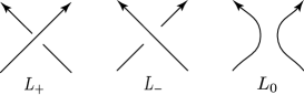
Figure 1. Figures in three small disks for $L_{+}$, $L_{-}$, and $L_{0}$.

Then the Jones polynomial $V_{L}$ is defined by

$$V_{\text{unknot}}(q)=q+q^{-1},$$

$$q^{-2}V_{L_{+}}(q)-q^{2}V_{L_{-}}(q)=(q^{-1}-q)V_{L_{0}}(q).$$

In the same way as the above, for a given unoriented link diagram $D$, using Fig. 2, we define three link diagrams corresponding to figures $D_{\times}$, $D_{0}$, and $D_{\infty}$.

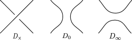
Figure 2. Figures in three small disks for $D_{\times}$, $D_{0}$, and $D_{\infty}$.

Then, for a link diagram $D$, the Kauffman bracket $\langle D\rangle\in\mathbb{Z}[A,A^{-1}]$ is defined by

(1) $$\langle~{}\begin{picture}(5.0,5.0)\put(3.0,3.0){\circle{9.0}} \end{picture}~{}\rangle=-A^{2}-A^{-2},$$

(2) $$\langle D\sqcup\ \begin{picture}(5.0,5.0)\put(3.0,3.0){\circle{9.0}} \end{picture}~{}\rangle=(-A^{2}-A^{-2})\langle D\rangle,$$

(3) $$\langle D_{\times}\rangle=A\langle D_{0}\rangle+A^{-1}\langle D_{\infty}\rangle.$$

Let $n_{+}$ ($n_{-}$, resp.) be the number of positive (negative, resp.) crossings, and let $w(D)=n_{+}-n_{-}$. It is known that for a link diagram $D$,

(4) $$V_{L}(-A^{-2})=(-A)^{-3w(D)}\langle D\rangle.$$

Using (3), the Kauffman bracket of $D$ is expressed as a linear sum of Kauffman brackets of an arrangement of circles on a plane. Then, each arrangement of circles on the plane is called a state.

Here, we reinterpret a state as a configuration of sufficiently small edges, each of which is on a crossing, called a marker. We denote a state by $s$. Then $D_{0}$ and $D_{\infty}$ are expressed by a marker on $D_{\times}$ (Fig. 3), i.e. $D_{0}$ ($D_{\infty}$, resp.) is obtained from $D_{\times}$ by smoothing of a crossing along a marker as in Fig. 3. We say that a marker corresponding to $D_{0}$ ($D_{\infty}$, resp.) is positive (negative, resp.). For a state $s$, the number of positive (negative, resp.) markers is denoted by $\sigma_{+}(s)$ ($\sigma_{-}(s)$, resp.).

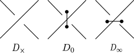
Figure 3. Markers on crossings.

Let $\sigma(s)=\sigma_{+}(s)-\sigma_{-}(s)$ and let $|s|$ be the number of circles in $s$. By definition,

$$\langle D\rangle=\sum_{s}A^{\sigma(s)}(-A^{-2}-A^{2})^{|s|}.$$

In [9], Viro introduced a refinement of a state by attaching signs to circles in $s$. An enhanced state $S$ is a state $s$ together with a choice of $+/-$-sign for each circle. Each circle in an enhanced state is called a state circle. Let $\tau_{+}(S)$ ($\tau_{-}(S)$, resp.) be the number of circles labeled $+$ ($-$, resp.) in $S$. Let $\tau(S)=\tau_{-}(S)-\tau_{+}(S)$. Let $\sigma(S)$ $=$ $\sigma(s)$ if $S$ is an enhanced state for a state $s$. Then, noting that $\tau(S)\equiv|s|$ (mod $2$), we have

$$\langle D\rangle =\sum_{s}A^{\sigma(s)}(-A^{2}-A^{-2})^{|s|}$$

(5) $$=\sum_{S}(-1)^{\tau(S)}A^{\sigma(S)-2\tau(S)}.$$

For an enhanced state $S$ of an oriented diagram $D$, let $i(S)$ $=$ $(w(D)-\sigma(S))/2$ and let $j(S)$ $=$ $w(D)+i(S)+\tau(S)$ $=$ $(3w(D)-\sigma(D)+2\tau(S))/2$. By (4) and (2.2), we have

$$\begin{split}V_{L}(q)|_{q=-A^{-2}}&=(-A)^{-3w(D)}\langle D\rangle\\ &=\sum_{S}(-1)^{-3w(D)+\tau(D)}A^{-3w(D)+\sigma(S)-2\tau(S)}\\ &=\sum_{S}(-1)^{w(D)+\tau(D)}(A^{-2})^{w(D)+(w(D)-\sigma(S))/2+\tau(S)}\\ &=\sum_{S}(-1)^{(w(D)-\sigma(S))/2}(-A^{-2})^{w(D)+(w(D)-\sigma(S))/2+\tau(S)}\\ &=\sum_{S}(-1)^{(w(D)-\sigma(S))/2}q^{w(D)+(w(D)-\sigma(S))/2+\tau(S)}\\ &=\sum_{S}(-1)^{i(S)}q^{j(S)}.\end{split}$$

Thus, each coefficient of $V_{L}(q)$ is the Euler characteristic.

2.3. Khovanov homologies for the Jones polynomial and the Kauffman bracket

Using [9], we give a review of the definitions of Khovanov homologies.

Definition 2.1 (oriented enhanced states and $C^{i,j}(D)$).

For an enhanced state, an orientation of a state is an ordering of the negative markers up to even permutation, where orientations that differ by odd permutations are considered opposite. For two enhanced states, we define a relation such that one enhanced state equals the other enhanced state multiplied by $-1$ ($1$, resp.) if they are the same enhanced states but with opposite (the same, resp.) orientations. Enhanced states with orientations are called oriented enhanced states. Then, for a link diagram $D$, let $C^{i,j}(D)$ be the free abelian group generated by oriented enhanced states with $i(S)=i$ and $j(S)=j$.

We introduce a notation [3, Page 1215] of elements of $C^{i,j}(D)$ as follows.

Notation 1 (a notation of elements in $C^{i,j}(D)$).

Let $\mathbb{L}$ be the set of crossings with negative markers of an enhanced state $S$ of a link diagram $D$, $C^{i,j}_{\mathbb{L}}(D)$ the free abelian group generated by the enhanced states having $\mathbb{L}$ with $i(S)=i$ and $j(S)=j$, and $E(\mathbb{L})$ the free abelian group generated by bijections from $\{1,2,\dots,\sharp\mathbb{L}\}$ to $\mathbb{L}$, where $\sharp\mathbb{L}$ is the cardinality of $\mathbb{L}$. For $f,g\in E(\mathbb{L})$, $p(f,g)$ is $-1$ ($1$, resp.) if $f^{-1}g$ is an odd (even, resp.) permutation. Then, let $F(\mathbb{L})=E(\mathbb{L})/(p(f,g)f-g)$. By definition, $C^{i,j}(D)$ is identified with $\bigoplus_{\mathbb{L},\sharp\mathbb{L}=n(i)}C^{i,j}_{\mathbb{L}}(D)\otimes F(\mathbb{L})$, where $n(i)$ denotes $\sharp\mathbb{L}$ when we fix $i$.

Throughout this paper, we freely use the identification.

Example 2.2.

By Notation 1, for a link diagram as in the first line of Fig. 4, the oriented enhanced states considered are represented as in the third line.

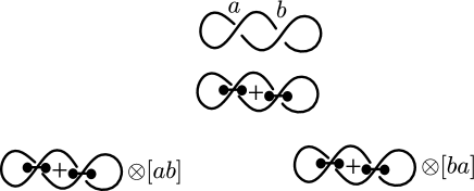
Figure 4. A knot diagram with two crossings $a$ and $b$ (1st line), an enhanced state $S$ of the knot diagram (2nd line), and the same enhanced states with opposite orientations (3rd line).

The notation “$ab$” or “$ba$” gives an order of the crossings with negative markers. The square bracket denotes an equivalence class including an order. For this example, we have $[ab]$ $=$ $-[ba]$.

Definition 2.3 (coboundary operator).

Let $x$ be a sequence of crossings with negative markers and $S$ and $T$ enhanced states. Let $a$ be a crossing with a positive marker of $S$. For $S\otimes[x]$ and $T\otimes[xa]$, if a pair $S$, $T$ appears as the figures in Fig. 5, $(S:T)$ is $1$; otherwise $(S:T)$ is $0$ as in the last line of Fig. 5. The number $(S:T)$ is called the incidence number of the pair of $S$, $T$. Then, a coboundary operator $d^{i}:C^{i,j}(D)\to C^{i+1,j}(D)$ is defined by

$$d^{i}(S\otimes[x])=\sum_{a}(S:T)\,T\otimes[xa].$$

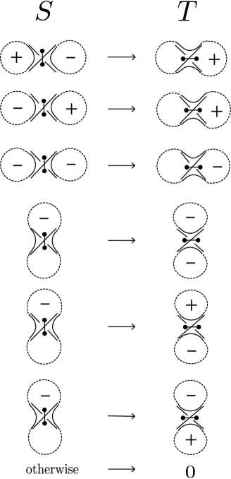
Figure 5. The definition of incidence numbers for enhanced states $S$ and $T$. The dotted arcs indicate how arcs of $S$ or $T$ are connected.

Here, recall (2.2):

$$\langle D\rangle =\sum_{S}(-1)^{\tau(S)}A^{\sigma(S)-2\tau(S)}.$$

Let $\mathcal{I}(S)$ $=$ $\tau(S)$ and let $\mathcal{J}(S)$ $=$ $\sigma(S)-2\tau(S)$. For a link diagram $D$, let $C_{\mathcal{I},\mathcal{J}}(D)$ be the free abelian group generated by oriented enhanced states with $\mathcal{I}(S)=\mathcal{I}$ and $\mathcal{J}(S)=\mathcal{J}$.

Definition 2.4 (chain group $C_{\mathcal{I},\mathcal{J}}(D)$).

Let $\mathbb{L}$ be the set of crossings with negative markers of an enhanced state $S$ of a link diagram $D$, and let $C_{\mathcal{I},\mathcal{J},\mathbb{L}}(D)$ be the free abelian group generated by enhanced states having $\mathbb{L}$ with $\mathcal{I}(S)=\mathcal{I}$ and $\mathcal{J}(S)=\mathcal{J}$. Then, let $C_{\mathcal{I},\mathcal{J}}(D)=\bigoplus_{\mathbb{L},\sharp\mathbb{L}=n(\mathcal{J}+2\mathcal{I})}C_{\mathcal{I},\mathcal{J},\mathbb{L}}(D)\otimes F(\mathbb{L})$ where $n(\mathcal{J}+2\mathcal{I})$ denotes $\sharp\mathbb{L}$ when we fix $\mathcal{J}+2\mathcal{I}$ (note that $\mathcal{J}(S)+2\mathcal{I}(S)=\sigma(S)$).

Definition 2.5 (boundary operator).

Let $x$ be a sequence of crossings with negative markers and $S$ and $T$ enhanced states. Let $a$ be a crossing with a positive marker of $S$. For $S\otimes[x]$ and $T\otimes[xa]$, if a pair $S$, $T$ appears as in Fig. 5, $(S:T)$ is $1$; otherwise $(S:T)$ is $0$ as in the last line of Fig. 5. The number $(S:T)$ is called the incidence number of the pair of $S$, $T$. Then, a boundary operator $\partial_{\mathcal{I}}:C_{\mathcal{I},\mathcal{J}}(D)\to C_{\mathcal{I}-1,\mathcal{J}}$ is defined by

$$\partial_{\mathcal{I}}(S\otimes[x])=\sum_{a}(S:T)\,T\otimes[xa].$$

Thanks to Khovanov [4], we have Fact 1.

Fact 1 (Khovanov).

The homology group $H^{i,j}(D)$ $(=H^{i}(C^{*,j}(D)))$ of a diagram $D$ of an oriented link $L$ is a link invariant, thus, it can be denoted by $H^{i,j}(L)$, such that

$$V_{L}(q)=\sum_{i,j}(-1)^{i}q^{j}{\rm{rank}}\,H^{i,j}(L).$$

Fact 2 (Khovanov, another grading of Viro [9]).

The homology group $H_{\mathcal{I},\mathcal{J}}(D)$ $(=H_{\mathcal{I}}(C_{*,\mathcal{J}}(D)))$ for a diagram $D$ of an unoriented framed link $L$ is a framed link invariant. Thus, it can be denoted by $H_{\mathcal{I},\mathcal{J}}(L)$ and

$$\langle D\rangle=\sum_{\mathcal{I},\mathcal{J}}(-1)^{\mathcal{I}}A^{\mathcal{J}}{\rm{rank}}\,H_{\mathcal{I},\mathcal{J}}(L).$$

3. Definition of a parametrized Khovanov homology

3.1. A parametrized Khovanov homology of the Jones polynomial

Definition 3.1 (a parametrized Khovanov homology of the Jones polynomial).

Let $D$ be an oriented link diagram and $C^{i,j}(D)$ a $\mathbb{Z}$-module of Notation 1. Let $\mathcal{C}^{i}(D)$ by $\mathcal{C}^{i}(D)$ $:=$ $\bigoplus_{j}C^{i,j}(D)$. Let $x$ be a sequence of crossings with negative markers, and $S$ and $T$ enhanced states. Then, let $a$ be a crossing with a positive marker of $S$ and let $(S:T)\in\mathbb{Z}[s,t]$. For $S\otimes[x]$ and $T\otimes[xa]$, if $S$ appears in a left-hand side of an arrow of Fig. 6, $(S:T)\,T$ is defined by the right-hand side of this arrow of Fig. 6. Then, a linear map $\delta^{i}_{s,t}:\mathcal{C}^{i}$ $\to$ $\mathcal{C}^{i+1}$ is defined by

$$\delta^{i}_{s,t}(S\otimes[x]):=\sum_{a}(S:T)\,T\otimes[xa].$$

Thanks to Khovanov [5], it is known that $\{\mathcal{C}^{i}(D),\delta^{i}_{s,t}\}_{i\in\mathbb{Z}}$ becomes a chain complex. In particular, $\delta^{i+1}_{s,t}\circ\delta^{i}_{s,t}=0$.

(6)

(7)

(8)

(9)

(10)

(11)

Figure 6. A generalized Frobenius calculus of signed circles.

Remark 3.2.

The case $s$ $=$ $t$ $=$ $0$ ($s$ $=$ $0$ and $t$ $=$ $1$ with the coefficient $\mathbb{Q}$, resp.) corresponds to the ordinary Khovanov homology (Lee homology, resp.).

3.2. A parametrized Khovanov homology of the Kauffman bracket

In order to define a parametrized Khovanov homology of the Kauffman bracket, for technical reasons , we need to redefine a grading of an “unparametrized” Khovanov homology in the same manner as in the preprint version [10] of [9].

Recalling (2.2):

$$\langle D\rangle =\sum_{S}(-1)^{\tau(S)}A^{\sigma(S)-2\tau(S)},$$

we switch the variable $A$ to $(-1)^{\frac{1}{2}}A$. Then,

$$\langle D\rangle =\sum_{S}(-1)^{\frac{\sigma(S)}{2}}A^{\sigma(S)-2\tau(S)}.$$

Let $I(S)$ $=$ $\frac{\sigma(S)}{2}$ and let $J(S)$ $=$ $\sigma(S)-2\tau(S)$. For a link diagram $D$, let $C_{I,J}(D)$ be the free abelian group generated by oriented enhanced states with $I(S)=I$ and $J(S)=J$. An orientation of an enhanced state is exhibited by $F(\mathbb{L})$ (Definition 2.4).

Definition 3.3 (chain group $C_{I,J}(D)$).

Let $\mathbb{L}$ be the set of crossings with negative markers of an enhanced state $S$ of a link diagram $D$, and let $C_{I,J,\mathbb{L}}(D)$ be the free abelian group generated by enhanced states having $\mathbb{L}$ with $I(S)=I$ and $J(S)=J$. Then, let $C_{I,J}(D)=\bigoplus_{\mathbb{L},\sharp\mathbb{L}=n(I)}C_{I,J,\mathbb{L}}(D)\otimes F(\mathbb{L})$ where $n(I)$ denotes $\sharp\mathbb{L}$ when we fix $I$.

If one orients the link diagram $D$, the chain groups $\mathcal{C}^{i,j}(D)$ appear, and

(12) $$C_{I,J}(D)=C^{\frac{w(D)}{2}-\mathcal{I},\frac{3w(D)-\mathcal{J}}{2}}(D).$$

Under this identification, the coboundary operator $\{d^{i}\}_{i\in\mathbb{Z}}$ (Definition 2.3) turns into a boundary operator $\{\partial_{I}\}_{I\in\mathbb{Z}}$. This $\{\partial_{I}\}_{I\in\mathbb{Z}}$ corresponds to an “unparametrized” case, which will be extended to Definition 3.4.

Definition 3.4 (a parametrized Khovanov homology of the Kauffman bracket).

Let $D$ be a link diagram and $C_{I,J}(D)$ is a $\mathbb{Z}$-module of Definition 3.3. Let $\mathcal{C}_{I}(D)$ $:=$ $\bigoplus_{J}C_{I,J}(D)$. Let $x$ be a sequence of crossings with negative markers and $S$ and $T$ enhanced states. Then, let $a$ be a crossing with a positive marker of $S$ and let $(S:T)$ be an integer. For $S\otimes[x]$ and $T\otimes[xa]$, if $S$ appears in a left-hand side of an arrow of Fig. 6, $(S:T)\,T$ is defined by the right-hand side of this arrow of Fig. 6. Then, a linear map $\delta_{I,s,t}:\mathcal{C}_{I}$ $\to$ $\mathcal{C}_{I-1}$ is defined by

$$\delta_{I,s,t}(S\otimes[x]):=\sum_{a}(S:T)\,T\otimes[xa].$$

Using the identification (12), for a link diagram $D$, the complex $\{\mathcal{C}^{i}(D),\delta^{i}_{s,t}\}_{i\in\mathbb{Z}}$ turns into the complex $\{\mathcal{C}_{I}(D),\delta_{I,s,t}\}_{I\in\mathbb{Z}}$. In particular, $\delta_{I-1,s,t}\circ\delta_{I,s,t}$ $=$ $0$.

4. Invariance parametrized Khovanov homology

By constructions in Sec. 3, below, we will show the invariance of homology groups of $\{\mathcal{C}^{i}(D),\delta^{i}_{s,t}\}_{i\in\mathbb{Z}}$ since the proof for $\{\mathcal{C}_{I}(D),\delta_{I,s,t}\}_{I\in\mathbb{Z}}$ is parallel to that of $\{\mathcal{C}^{i}(D),\delta^{i}_{s,t}\}_{i\in\mathbb{Z}}$ except for replacing $i$ with $I$ by (12).

Before starting proofs, we prepare notations and a definition.

Notation 2 ($p:q$, $q:p$, and $m(p:q)$ [3] ).

Let $p$ and $q$ be signs ($+$ or $-$) on circles in an enhanced state. The coboundary map $\delta_{s,t}$ (Definition 3.1) is denoted by

(13) $$\begin{minipage}{50.0pt} \begin{picture}(50.0,50.0)\put(0.0,10.0){\line(1,1){30.0}} \qbezier(30.0,10.0)(30.0,10.0)(20.0,20.0)\qbezier(10.0,30.0)(0.0,40.0)(0.0,40.0) \put(15.0,15.0){\circle*{5.0}} \put(15.0,35.0){\circle*{5.0}} \put(15.0,15.0){\line(0,1){20.0}} \put(22.0,23.0){$q$} \put(3.0,23.0){$p$} \put(13.0,5.0){$a$} \end{picture} \end{minipage}\otimes[x]\qquad\longmapsto\qquad\quad\quad\begin{minipage}{50.0pt} \begin{picture}(50.0,50.0)\put(0.0,10.0){\line(1,1){30.0}} \qbezier(30.0,10.0)(30.0,10.0)(20.0,20.0)\qbezier(10.0,30.0)(0.0,40.0)(0.0,40.0) \put(5.0,25.0){\circle*{5.0}} \put(25.0,25.0){\circle*{5.0}} \put(5.0,25.0){\line(1,0){20.0}} \put(5.0,40.0){$p:q$} \put(5.0,5.0){$q:p$} \put(30.0,23.0){$a$} \end{picture} \end{minipage}\ \ \otimes[xa]$$

with symbols $p:q$ and $q:p$ using correspondences as in Fig. 6. When it is convenient to specify that $p:q$ is of multiplication (Fig. 6, (6)–(9)), we shall denote $p:q$ by $m(p:q)$.

Note also that $\begin{minipage}{50.0pt} \begin{picture}(50.0,50.0)\put(0.0,10.0){\line(1,1){30.0}} \qbezier(30.0,10.0)(30.0,10.0)(20.0,20.0)\qbezier(10.0,30.0)(0.0,40.0)(0.0,40.0) \put(5.0,25.0){\circle*{5.0}} \put(25.0,25.0){\circle*{5.0}} \put(5.0,25.0){\line(1,0){20.0}} \put(5.0,40.0){$p:q$} \put(5.0,5.0){$q:p$} \put(30.0,23.0){$a$} \end{picture} \end{minipage}\otimes[xa]=\begin{minipage}{50.0pt} \begin{picture}(50.0,50.0)\put(0.0,10.0){\line(1,1){30.0}} \qbezier(30.0,10.0)(30.0,10.0)(20.0,20.0)\qbezier(10.0,30.0)(0.0,40.0)(0.0,40.0) \put(5.0,25.0){\circle*{5.0}} \put(25.0,25.0){\circle*{5.0}} \put(5.0,25.0){\line(1,0){20.0}} \put(5.0,40.0){$q:p$} \put(5.0,5.0){$p:q$} \put(30.0,23.0){$a$} \end{picture} \end{minipage}\otimes[xa]$, i.e. $\begin{minipage}{40.0pt} \begin{picture}(0.0,60.0)\put(10.0,42.0){$p:q$} \qbezier(5.0,40.0)(20.0,25.0)(35.0,40.0)\qbezier(5.0,15.0)(20.0,30.0)(35.0,15.0)\put(10.0,10.0){$q:p$} \end{picture} \end{minipage}=\begin{minipage}{40.0pt} \begin{picture}(0.0,60.0)\put(10.0,42.0){$q:p$} \qbezier(5.0,40.0)(20.0,25.0)(35.0,40.0)\qbezier(5.0,15.0)(20.0,30.0)(35.0,15.0)\put(10.0,10.0){$p:q$} \end{picture} \end{minipage}$ as in Fig. 6. Throughout this paper, we freely use this property of $(p:q,q:p)$.

Notation 3 ($\mathcal{C}(S_{1},S_{2},\dots,S_{n})$).

Let $D$ be a link diagram and $\mathcal{C}^{i}(D)$ a chain group as in Definition 3.1. By definition, $\mathcal{C}^{i}(D)$ is a $\mathbb{Z}$-module. When we do not need to specify the index $i$, we denote it by $\mathcal{C}(D)$ simply. Then, we denote by $\mathcal{C}(S_{1},S_{2},\dots,S_{n})$ a sub-module spanned by $S_{1},S_{2},\dots,S_{n}\in\mathcal{C}(D)$.

Example 4.1.

Let $p$ be a sign of a state circle. By Fig. 6, it is easy to see that $m(p:-)$ $=$ $p$. It is also easy to see that after splitting a circle with the sign $p$, if the sign of a circle is $+$, the other is $p$.

Definition 4.2 (Reidemeister moves).

Let $D$ be a link diagram ($\subset\mathbb{R}^{2}$). The left-twisted first Reidemeister move is a replacement of a sufficiently small disk $U_{1}$ $=$ with another one $U^{\prime}_{1}$ $=$ and its inverse, where $\mathbb{R}^{2}\setminus U_{1}$ $=$ $\mathbb{R}^{2}\setminus U^{\prime}_{1}$. The second Reidemeister move is a replacement of a sufficiently small disk $U_{2}$ $=$ with another one $U^{\prime}_{2}$ $=$ and its inverse, where $\mathbb{R}^{2}\setminus U_{2}$ $=$ $\mathbb{R}^{2}\setminus U^{\prime}_{2}$. The third Reidemeister move is a replacement of a sufficiently small disk $U_{3}$ $=$ with another one $U^{\prime}_{3}$ $=$ and its inverse, where $\mathbb{R}^{2}\setminus U_{3}$ $=$ $\mathbb{R}^{2}\setminus U^{\prime}_{3}$. For an oriented link diagram $D$, each equality $\mathbb{R}^{2}\setminus U_{i}$ $=$ $\mathbb{R}^{2}\setminus U^{\prime}_{i}$ ($i=1,2,3$) induces the orientation of $D^{\prime}$.

One may worry about other moves. Note that the right-twisted first Reidemeister move is generated by the left-twisted first and the second Reidemeister moves. Note also that the local move between and is realized by a sequence of the second Reidemeister moves and the third Reidemeister move. Therefore, in Sec. 4.1–Sec. 4.3, we will show the invariances of the left-twisted first, the second, and the third Reidemeister moves as in Definition 4.2.

4.1. The invariance under the left-twisted first Reidemeister move

Let $D$ and $D^{\prime}$ be two link diagrams which are related by a left-twisted first Reidemeister move at a crossing “$a$”, and $D$ is represented by   and $D^{\prime}$ is represented by . Let $x$ be a sequence of crossings with negative markers. Let $\mathcal{C}$ be a $\mathbb{Z}$-module generated by enhanced states of type

(14) $$\begin{minipage}{30.0pt} \begin{picture}(30.0,30.0)\qbezier(6.6,17.0)(0.0,24.0)(0.0,24.0)\qbezier(0.0,4.0)(20.0,34.0)(25.0,17.0)\qbezier(11.0,13.0)(20.0,4.0)(24.5,12.0)\qbezier(24.5,12.0)(25.5,14.5)(25.0,17.0){\color[rgb]{0,0,0}{\put(8.0,19.5){\circle*{3.0}} \put(8.0,10.5){\circle*{3.0}} \put(8.0,11.5){\line(0,1){8.0}}}} \put(-3.5,12.5){\text{$p$}} \put(14.0,12.5){\text{$+$}} \end{picture} \end{minipage}\!\!\otimes[x]-m(p:+)\begin{minipage}{30.0pt} \begin{picture}(30.0,30.0)\qbezier(6.6,17.0)(0.0,24.0)(0.0,24.0)\qbezier(0.0,4.0)(20.0,34.0)(25.0,17.0)\qbezier(11.0,13.0)(20.0,4.0)(24.5,12.0)\qbezier(24.5,12.0)(25.5,14.5)(25.0,17.0){\color[rgb]{0,0,0}{\put(8.0,19.5){\circle*{3.0}} \put(8.0,10.5){\circle*{3.0}} \put(8.0,11.5){\line(0,1){8.0}}}} \put(14.0,12.5){\text{$-$}} \end{picture} \end{minipage}\!\!\otimes[x]\quad(p=+,-),$$

where the second term is fixed by the first term in (14). Let $\mathcal{C}_{\rm{contr}}$ be a $\mathbb{Z}$-module generated by enhanced states of types

$$\begin{minipage}{30.0pt} \begin{picture}(30.0,30.0)\qbezier(6.6,17.0)(0.0,24.0)(0.0,24.0)\qbezier(0.0,4.0)(20.0,34.0)(25.0,17.0)\qbezier(11.0,13.0)(20.0,4.0)(24.5,12.0)\qbezier(24.5,12.0)(25.5,14.5)(25.0,17.0){\color[rgb]{0,0,0}{\put(8.0,19.5){\circle*{3.0}} \put(8.0,10.5){\circle*{3.0}} \put(8.0,11.5){\line(0,1){8.0}}}} \put(-3.5,12.5){\text{$p$}} \put(14.0,12.5){\text{$-$}} \end{picture} \end{minipage}\!\!\otimes[x]\quad(p=+,-),\begin{minipage}{30.0pt} \begin{picture}(30.0,30.0)\qbezier(6.6,17.0)(0.0,24.0)(0.0,24.0)\qbezier(0.0,4.0)(20.0,34.0)(25.0,17.0)\qbezier(11.0,13.0)(20.0,4.0)(24.5,12.0)\qbezier(24.5,12.0)(25.5,14.5)(25.0,17.0){\color[rgb]{0,0,0}{\put(12.5,15.5){\circle*{3.0}} \put(4.5,15.5){\circle*{3.0}} \put(4.5,15.5){\line(1,0){8.0}}}} \put(15.5,14.0){\text{$p$}} \end{picture} \end{minipage}\!\!\otimes[xa]\quad(p=+,-).$$

Lemma 4.3.

(15) $$\mathcal{C}(D)=\mathcal{C}\oplus\mathcal{C}_{\rm{contr}},$$

where each of $\mathcal{C}$ and $\mathcal{C}_{\rm{contr}}$ is a subcomplex of $\mathcal{C}(D)$.

Before starting the proof, we prepare a notation.

Notation 4.

Let $p_{u}$ be the sign induced from a sign $p$ by changing a marker on a crossing $u$ when we apply $\delta_{s,t}$ (13). By definition, $p_{u}=p$ if a new marker on $u$ cannot affect a state circle with $p$. For example, if $p$ $=$ $m(p:+)$, we denote $p_{u}$ by $(m(p:+))_{u}$.

Proof.

Let $p_{u}$ be a sign as in Notation 4.

$$\delta_{s,t}\left(~{}~{}\begin{minipage}{30.0pt} \begin{picture}(30.0,30.0)\qbezier(6.6,17.0)(0.0,24.0)(0.0,24.0)\qbezier(0.0,4.0)(20.0,34.0)(25.0,17.0)\qbezier(11.0,13.0)(20.0,4.0)(24.5,12.0)\qbezier(24.5,12.0)(25.5,14.5)(25.0,17.0){\color[rgb]{0,0,0}{\put(8.0,19.5){\circle*{3.0}} \put(8.0,10.5){\circle*{3.0}} \put(8.0,11.5){\line(0,1){8.0}}}} \put(-3.5,12.5){\text{$p$}} \put(14.0,12.5){\text{$+$}} \end{picture} \end{minipage}\!\!\otimes[x]-m(p:+)\begin{minipage}{30.0pt} \begin{picture}(30.0,30.0)\qbezier(6.6,17.0)(0.0,24.0)(0.0,24.0)\qbezier(0.0,4.0)(20.0,34.0)(25.0,17.0)\qbezier(11.0,13.0)(20.0,4.0)(24.5,12.0)\qbezier(24.5,12.0)(25.5,14.5)(25.0,17.0){\color[rgb]{0,0,0}{\put(8.0,19.5){\circle*{3.0}} \put(8.0,10.5){\circle*{3.0}} \put(8.0,11.5){\line(0,1){8.0}}}} \put(14.0,12.5){\text{$-$}} \end{picture} \end{minipage}\!\!\otimes[x]\right)$$

$$=\sum_{u}~{}\left(~{}\begin{minipage}{30.0pt} \begin{picture}(30.0,30.0)\qbezier(6.6,17.0)(0.0,24.0)(0.0,24.0)\qbezier(0.0,4.0)(20.0,34.0)(25.0,17.0)\qbezier(11.0,13.0)(20.0,4.0)(24.5,12.0)\qbezier(24.5,12.0)(25.5,14.5)(25.0,17.0){\color[rgb]{0,0,0}{\put(8.0,19.5){\circle*{3.0}} \put(8.0,10.5){\circle*{3.0}} \put(8.0,11.5){\line(0,1){8.0}}}} \put(-5.0,13.5){\text{$p_{u}$}} \put(14.0,12.5){\text{$+$}} \end{picture} \end{minipage}\!\!\otimes[xu]-(m(p:+))_{u}\begin{minipage}{30.0pt} \begin{picture}(30.0,30.0)\qbezier(6.6,17.0)(0.0,24.0)(0.0,24.0)\qbezier(0.0,4.0)(20.0,34.0)(25.0,17.0)\qbezier(11.0,13.0)(20.0,4.0)(24.5,12.0)\qbezier(24.5,12.0)(25.5,14.5)(25.0,17.0){\color[rgb]{0,0,0}{\put(8.0,19.5){\circle*{3.0}} \put(8.0,10.5){\circle*{3.0}} \put(8.0,11.5){\line(0,1){8.0}}}} \put(14.0,12.5){\text{$-$}} \end{picture} \end{minipage}\!\!\otimes[xu]\right)$$

$$=\sum_{u}~{}\left(~{}\begin{minipage}{30.0pt} \begin{picture}(30.0,30.0)\qbezier(6.6,17.0)(0.0,24.0)(0.0,24.0)\qbezier(0.0,4.0)(20.0,34.0)(25.0,17.0)\qbezier(11.0,13.0)(20.0,4.0)(24.5,12.0)\qbezier(24.5,12.0)(25.5,14.5)(25.0,17.0){\color[rgb]{0,0,0}{\put(8.0,19.5){\circle*{3.0}} \put(8.0,10.5){\circle*{3.0}} \put(8.0,11.5){\line(0,1){8.0}}}} \put(-5.0,13.5){\text{$p_{u}$}} \put(14.0,12.5){\text{$+$}} \end{picture} \end{minipage}\!\!\otimes[xu]-m(p_{u}:+)\begin{minipage}{30.0pt} \begin{picture}(30.0,30.0)\qbezier(6.6,17.0)(0.0,24.0)(0.0,24.0)\qbezier(0.0,4.0)(20.0,34.0)(25.0,17.0)\qbezier(11.0,13.0)(20.0,4.0)(24.5,12.0)\qbezier(24.5,12.0)(25.5,14.5)(25.0,17.0){\color[rgb]{0,0,0}{\put(8.0,19.5){\circle*{3.0}} \put(8.0,10.5){\circle*{3.0}} \put(8.0,11.5){\line(0,1){8.0}}}} \put(14.0,12.5){\text{$-$}} \end{picture} \end{minipage}\!\!\otimes[xu]\right)\in\mathcal{C},$$

$$\delta_{s,t}\left(~{}\begin{minipage}{30.0pt} \begin{picture}(30.0,30.0)\qbezier(6.6,17.0)(0.0,24.0)(0.0,24.0)\qbezier(0.0,4.0)(20.0,34.0)(25.0,17.0)\qbezier(11.0,13.0)(20.0,4.0)(24.5,12.0)\qbezier(24.5,12.0)(25.5,14.5)(25.0,17.0){\color[rgb]{0,0,0}{\put(8.0,19.5){\circle*{3.0}} \put(8.0,10.5){\circle*{3.0}} \put(8.0,11.5){\line(0,1){8.0}}}} \put(-3.5,12.5){\text{$p$}} \put(14.0,12.5){\text{$-$}} \end{picture} \end{minipage}\!\!\otimes[x]\right)=\begin{minipage}{30.0pt} \begin{picture}(30.0,30.0)\qbezier(6.6,17.0)(0.0,24.0)(0.0,24.0)\qbezier(0.0,4.0)(20.0,34.0)(25.0,17.0)\qbezier(11.0,13.0)(20.0,4.0)(24.5,12.0)\qbezier(24.5,12.0)(25.5,14.5)(25.0,17.0){\color[rgb]{0,0,0}{\put(12.5,15.5){\circle*{3.0}} \put(4.5,15.5){\circle*{3.0}} \put(4.5,15.5){\line(1,0){8.0}}}} \put(15.5,14.0){\text{$p$}} \end{picture} \end{minipage}\!\!\otimes[xa]+\!\sum_{u}~{}~{}\begin{minipage}{30.0pt} \begin{picture}(30.0,30.0)\qbezier(6.6,17.0)(0.0,24.0)(0.0,24.0)\qbezier(0.0,4.0)(20.0,34.0)(25.0,17.0)\qbezier(11.0,13.0)(20.0,4.0)(24.5,12.0)\qbezier(24.5,12.0)(25.5,14.5)(25.0,17.0){\color[rgb]{0,0,0}{\put(8.0,19.5){\circle*{3.0}} \put(8.0,10.5){\circle*{3.0}} \put(8.0,11.5){\line(0,1){8.0}}}} \put(-4.8,13.0){\text{$p_{u}$}} \put(14.0,12.5){\text{$-$}} \end{picture} \end{minipage}\!\!\otimes[xu]\in\mathcal{C}_{\rm{contr}}$$

(the last equality holds since $\delta_{s,t}$ is the coboundary operator, e.g. [9, 5.3.A]), and

$$\delta_{s,t}\left(\begin{minipage}{30.0pt} \begin{picture}(30.0,30.0)\qbezier(6.6,17.0)(0.0,24.0)(0.0,24.0)\qbezier(0.0,4.0)(20.0,34.0)(25.0,17.0)\qbezier(11.0,13.0)(20.0,4.0)(24.5,12.0)\qbezier(24.5,12.0)(25.5,14.5)(25.0,17.0){\color[rgb]{0,0,0}{\put(12.5,15.5){\circle*{3.0}} \put(4.5,15.5){\circle*{3.0}} \put(4.5,15.5){\line(1,0){8.0}}}} \put(15.5,14.0){\text{$p$}} \end{picture} \end{minipage}\!\!\otimes[xa]\right)=\sum_{u}~{}\begin{minipage}{30.0pt} \begin{picture}(30.0,30.0)\qbezier(6.6,17.0)(0.0,24.0)(0.0,24.0)\qbezier(0.0,4.0)(20.0,34.0)(25.0,17.0)\qbezier(11.0,13.0)(20.0,4.0)(24.5,12.0)\qbezier(24.5,12.0)(25.5,14.5)(25.0,17.0){\color[rgb]{0,0,0}{\put(12.5,15.5){\circle*{3.0}} \put(4.5,15.5){\circle*{3.0}} \put(4.5,15.5){\line(1,0){8.0}}}} \put(15.0,15.0){\text{$p_{u}$}} \end{picture} \end{minipage}\!\!\otimes[xau]\in\mathcal{C}_{\rm{contr}}.$$

∎

We consider the composition

$$\mathcal{C}(D)=\mathcal{C}\oplus\mathcal{C}_{\rm{contr}}\stackrel{{\scriptstyle\rho_{1}}}{{\to}}\mathcal{C}\stackrel{{\scriptstyle\operatorname{isom}_{1}}}{{\to}}\mathcal{C}(D^{\prime}),$$

which consists of the projection $\rho_{1}:$ $\mathcal{C}\oplus\mathcal{C}_{\rm{contr}}$ $\to$ $\mathcal{C}$ and

$$\operatorname{isom}_{1}:\mathcal{C}\left(~{}\begin{minipage}{30.0pt} \begin{picture}(30.0,30.0)\qbezier(6.6,17.0)(0.0,24.0)(0.0,24.0)\qbezier(0.0,4.0)(20.0,34.0)(25.0,17.0)\qbezier(11.0,13.0)(20.0,4.0)(24.5,12.0)\qbezier(24.5,12.0)(25.5,14.5)(25.0,17.0){\color[rgb]{0,0,0}{\put(8.0,19.5){\circle*{3.0}} \put(8.0,10.5){\circle*{3.0}} \put(8.0,11.5){\line(0,1){8.0}}}} \put(-3.5,12.5){\text{$p$}} \put(14.0,12.5){\text{$+$}} \end{picture} \end{minipage}\!\!\otimes[x]-m(p:+)\begin{minipage}{30.0pt} \begin{picture}(30.0,30.0)\qbezier(6.6,17.0)(0.0,24.0)(0.0,24.0)\qbezier(0.0,4.0)(20.0,34.0)(25.0,17.0)\qbezier(11.0,13.0)(20.0,4.0)(24.5,12.0)\qbezier(24.5,12.0)(25.5,14.5)(25.0,17.0){\color[rgb]{0,0,0}{\put(8.0,19.5){\circle*{3.0}} \put(8.0,10.5){\circle*{3.0}} \put(8.0,11.5){\line(0,1){8.0}}}} \put(14.0,12.5){\text{$-$}} \end{picture} \end{minipage}\!\!\otimes[x]\right)\to\mathcal{C}\left(~{}\begin{minipage}{30.0pt} \begin{picture}(30.0,30.0)\cbezier(0,3)(30,5)(30,25)(0,27) \end{picture} \end{minipage}\!\!\otimes[x]\right);$$

$$\begin{minipage}{30.0pt} \begin{picture}(30.0,30.0)\qbezier(6.6,17.0)(0.0,24.0)(0.0,24.0)\qbezier(0.0,4.0)(20.0,34.0)(25.0,17.0)\qbezier(11.0,13.0)(20.0,4.0)(24.5,12.0)\qbezier(24.5,12.0)(25.5,14.5)(25.0,17.0){\color[rgb]{0,0,0}{\put(8.0,19.5){\circle*{3.0}} \put(8.0,10.5){\circle*{3.0}} \put(8.0,11.5){\line(0,1){8.0}}}} \put(-3.5,12.5){\text{$p$}} \put(14.0,12.5){\text{$+$}} \end{picture} \end{minipage}\!\!\otimes[x]-m(p:+)\begin{minipage}{30.0pt} \begin{picture}(30.0,30.0)\qbezier(6.6,17.0)(0.0,24.0)(0.0,24.0)\qbezier(0.0,4.0)(20.0,34.0)(25.0,17.0)\qbezier(11.0,13.0)(20.0,4.0)(24.5,12.0)\qbezier(24.5,12.0)(25.5,14.5)(25.0,17.0){\color[rgb]{0,0,0}{\put(8.0,19.5){\circle*{3.0}} \put(8.0,10.5){\circle*{3.0}} \put(8.0,11.5){\line(0,1){8.0}}}} \put(14.0,12.5){\text{$-$}} \end{picture} \end{minipage}\!\!\otimes[x]\mapsto~{}\ \begin{minipage}{30.0pt} \begin{picture}(30.0,30.0)\cbezier(0,3)(30,5)(30,25)(0,27) \put(5.0,12.5){\text{$p$}} \end{picture} \end{minipage}\!\!\otimes[x].$$

Since $\rho_{1}$ is a projection, it is a chain map. We also have Lemma 4.4.

Lemma 4.4.

The linear map $\operatorname{isom}_{1}$ is a bijection and a chain map.

Proof.

Recall that the second term $m(p:+)\begin{minipage}{30.0pt} \begin{picture}(30.0,30.0)\qbezier(6.6,17.0)(0.0,24.0)(0.0,24.0)\qbezier(0.0,4.0)(20.0,34.0)(25.0,17.0)\qbezier(11.0,13.0)(20.0,4.0)(24.5,12.0)\qbezier(24.5,12.0)(25.5,14.5)(25.0,17.0){\color[rgb]{0,0,0}{\put(8.0,19.5){\circle*{3.0}} \put(8.0,10.5){\circle*{3.0}} \put(8.0,11.5){\line(0,1){8.0}}}} \put(14.0,12.5){\text{$-$}} \end{picture} \end{minipage}\!\!\otimes[x]$ is fixed by the first term $\begin{minipage}{30.0pt} \begin{picture}(35.0,30.0)\qbezier(6.6,17.0)(0.0,24.0)(0.0,24.0)\qbezier(0.0,4.0)(20.0,34.0)(25.0,17.0)\qbezier(11.0,13.0)(20.0,4.0)(24.5,12.0)\qbezier(24.5,12.0)(25.5,14.5)(25.0,17.0){\color[rgb]{0,0,0}{\put(8.0,19.5){\circle*{3.0}} \put(8.0,10.5){\circle*{3.0}} \put(8.0,11.5){\line(0,1){8.0}}}} \put(-1.5,12.5){\text{$p$}} \put(14.0,12.5){\text{$+$}} \end{picture} \end{minipage}\!\!\otimes[x]$. Then, it implies that $\begin{minipage}{30.0pt} \begin{picture}(35.0,30.0)\qbezier(6.6,17.0)(0.0,24.0)(0.0,24.0)\qbezier(0.0,4.0)(20.0,34.0)(25.0,17.0)\qbezier(11.0,13.0)(20.0,4.0)(24.5,12.0)\qbezier(24.5,12.0)(25.5,14.5)(25.0,17.0){\color[rgb]{0,0,0}{\put(8.0,19.5){\circle*{3.0}} \put(8.0,10.5){\circle*{3.0}} \put(8.0,11.5){\line(0,1){8.0}}}} \put(-1.5,12.5){\text{$p$}} \put(14.0,12.5){\text{$+$}} \end{picture} \end{minipage}\!\!\otimes[x]$ fixes $\begin{minipage}{30.0pt} \begin{picture}(30.0,30.0)\cbezier(0,3)(30,5)(30,25)(0,27) \put(5.0,12.5){\text{$p$}} \end{picture} \end{minipage}\!\!\otimes[x]$ for each sign $p$ by $\operatorname{isom}_{1}$. Conversely, $\begin{minipage}{30.0pt} \begin{picture}(30.0,30.0)\cbezier(0,3)(30,5)(30,25)(0,27) \put(5.0,12.5){\text{$p$}} \end{picture} \end{minipage}\!\!\otimes[x]$ also fixes $\begin{minipage}{30.0pt} \begin{picture}(35.0,30.0)\qbezier(6.6,17.0)(0.0,24.0)(0.0,24.0)\qbezier(0.0,4.0)(20.0,34.0)(25.0,17.0)\qbezier(11.0,13.0)(20.0,4.0)(24.5,12.0)\qbezier(24.5,12.0)(25.5,14.5)(25.0,17.0){\color[rgb]{0,0,0}{\put(8.0,19.5){\circle*{3.0}} \put(8.0,10.5){\circle*{3.0}} \put(8.0,11.5){\line(0,1){8.0}}}} \put(-1.5,12.5){\text{$p$}} \put(14.0,12.5){\text{$+$}} \end{picture} \end{minipage}\!\!\otimes[x]$, which implies that $\operatorname{isom}_{1}$ is a bijection.

Next, letting $p_{u}$ be as in Notation 4,

$$\delta_{s,t}\circ\operatorname{isom}_{1}\left(\begin{minipage}{30.0pt} \begin{picture}(30.0,30.0)\qbezier(6.6,17.0)(0.0,24.0)(0.0,24.0)\qbezier(0.0,4.0)(20.0,34.0)(25.0,17.0)\qbezier(11.0,13.0)(20.0,4.0)(24.5,12.0)\qbezier(24.5,12.0)(25.5,14.5)(25.0,17.0){\color[rgb]{0,0,0}{\put(8.0,19.5){\circle*{3.0}} \put(8.0,10.5){\circle*{3.0}} \put(8.0,11.5){\line(0,1){8.0}}}} \put(-3.5,12.5){\text{$p$}} \put(14.0,12.5){\text{$+$}} \end{picture} \end{minipage}\!\!\otimes[x]-m(p:+)\begin{minipage}{30.0pt} \begin{picture}(30.0,30.0)\qbezier(6.6,17.0)(0.0,24.0)(0.0,24.0)\qbezier(0.0,4.0)(20.0,34.0)(25.0,17.0)\qbezier(11.0,13.0)(20.0,4.0)(24.5,12.0)\qbezier(24.5,12.0)(25.5,14.5)(25.0,17.0){\color[rgb]{0,0,0}{\put(8.0,19.5){\circle*{3.0}} \put(8.0,10.5){\circle*{3.0}} \put(8.0,11.5){\line(0,1){8.0}}}} \put(14.0,12.5){\text{$-$}} \end{picture} \end{minipage}\!\!\otimes[x]\right) =\delta_{s,t}\left(\begin{minipage}{30.0pt} \begin{picture}(30.0,30.0)\cbezier(0,3)(30,5)(30,25)(0,27) \put(5.0,12.5){\text{$p$}} \end{picture} \end{minipage}\!\!\otimes[x]\right)$$

$$=\sum_{u}\begin{minipage}{30.0pt} \begin{picture}(30.0,30.0)\cbezier(0,3)(30,5)(30,25)(0,27) \put(5.0,12.5){\text{$p_{u}$}} \end{picture} \end{minipage}\!\!\otimes[xu],$$

and

$$\operatorname{isom}_{1}\circ\delta_{s,t}\left(~{}\begin{minipage}{30.0pt} \begin{picture}(30.0,30.0)\qbezier(6.6,17.0)(0.0,24.0)(0.0,24.0)\qbezier(0.0,4.0)(20.0,34.0)(25.0,17.0)\qbezier(11.0,13.0)(20.0,4.0)(24.5,12.0)\qbezier(24.5,12.0)(25.5,14.5)(25.0,17.0){\color[rgb]{0,0,0}{\put(8.0,19.5){\circle*{3.0}} \put(8.0,10.5){\circle*{3.0}} \put(8.0,11.5){\line(0,1){8.0}}}} \put(-3.5,12.5){\text{$p$}} \put(14.0,12.5){\text{$+$}} \end{picture} \end{minipage}\!\!\otimes[x]-m(p:+)\begin{minipage}{30.0pt} \begin{picture}(30.0,30.0)\qbezier(6.6,17.0)(0.0,24.0)(0.0,24.0)\qbezier(0.0,4.0)(20.0,34.0)(25.0,17.0)\qbezier(11.0,13.0)(20.0,4.0)(24.5,12.0)\qbezier(24.5,12.0)(25.5,14.5)(25.0,17.0){\color[rgb]{0,0,0}{\put(8.0,19.5){\circle*{3.0}} \put(8.0,10.5){\circle*{3.0}} \put(8.0,11.5){\line(0,1){8.0}}}} \put(14.0,12.5){\text{$-$}} \end{picture} \end{minipage}\!\!\otimes[x]\right)$$

$$=\operatorname{isom}_{1}\left(\sum_{u}~{}~{}~{}\begin{minipage}{30.0pt} \begin{picture}(30.0,30.0)\qbezier(6.6,17.0)(0.0,24.0)(0.0,24.0)\qbezier(0.0,4.0)(20.0,34.0)(25.0,17.0)\qbezier(11.0,13.0)(20.0,4.0)(24.5,12.0)\qbezier(24.5,12.0)(25.5,14.5)(25.0,17.0){\color[rgb]{0,0,0}{\put(8.0,19.5){\circle*{3.0}} \put(8.0,10.5){\circle*{3.0}} \put(8.0,11.5){\line(0,1){8.0}}}} \put(-4.0,14.0){\text{$p_{u}$}} \put(14.0,12.5){\text{$+$}} \end{picture} \end{minipage}\!\!\otimes[xu]-m(p_{u}:+)\begin{minipage}{30.0pt} \begin{picture}(30.0,30.0)\qbezier(6.6,17.0)(0.0,24.0)(0.0,24.0)\qbezier(0.0,4.0)(20.0,34.0)(25.0,17.0)\qbezier(11.0,13.0)(20.0,4.0)(24.5,12.0)\qbezier(24.5,12.0)(25.5,14.5)(25.0,17.0){\color[rgb]{0,0,0}{\put(8.0,19.5){\circle*{3.0}} \put(8.0,10.5){\circle*{3.0}} \put(8.0,11.5){\line(0,1){8.0}}}} \put(14.0,12.5){\text{$-$}} \end{picture} \end{minipage}\!\!\otimes[xu]\right)$$

$$=\sum_{u}\begin{minipage}{30.0pt} \begin{picture}(30.0,30.0)\cbezier(0,3)(30,5)(30,25)(0,27) \put(5.0,12.5){\text{$p_{u}$}} \end{picture} \end{minipage}\!\!\otimes[xu].$$

∎

Lemma 4.5.

$\rho_{1}$ is represented by

$$\begin{split}&\begin{minipage}{30.0pt} \begin{picture}(30.0,30.0)\qbezier(6.6,17.0)(0.0,24.0)(0.0,24.0)\qbezier(0.0,4.0)(20.0,34.0)(25.0,17.0)\qbezier(11.0,13.0)(20.0,4.0)(24.5,12.0)\qbezier(24.5,12.0)(25.5,14.5)(25.0,17.0){\color[rgb]{0,0,0}{\put(8.0,19.5){\circle*{3.0}} \put(8.0,10.5){\circle*{3.0}} \put(8.0,11.5){\line(0,1){8.0}}}} \put(-3.5,12.5){\text{$p$}} \put(14.0,12.5){\text{$+$}} \end{picture} \end{minipage}\!\!\otimes[x]\mapsto\ \begin{minipage}{30.0pt} \begin{picture}(30.0,30.0)\qbezier(6.6,17.0)(0.0,24.0)(0.0,24.0)\qbezier(0.0,4.0)(20.0,34.0)(25.0,17.0)\qbezier(11.0,13.0)(20.0,4.0)(24.5,12.0)\qbezier(24.5,12.0)(25.5,14.5)(25.0,17.0){\color[rgb]{0,0,0}{\put(8.0,19.5){\circle*{3.0}} \put(8.0,10.5){\circle*{3.0}} \put(8.0,11.5){\line(0,1){8.0}}}} \put(-3.5,12.5){\text{$p$}} \put(14.0,12.5){\text{$+$}} \end{picture} \end{minipage}\!\!\otimes[x]-m(p:+)\begin{minipage}{30.0pt} \begin{picture}(30.0,30.0)\qbezier(6.6,17.0)(0.0,24.0)(0.0,24.0)\qbezier(0.0,4.0)(20.0,34.0)(25.0,17.0)\qbezier(11.0,13.0)(20.0,4.0)(24.5,12.0)\qbezier(24.5,12.0)(25.5,14.5)(25.0,17.0){\color[rgb]{0,0,0}{\put(8.0,19.5){\circle*{3.0}} \put(8.0,10.5){\circle*{3.0}} \put(8.0,11.5){\line(0,1){8.0}}}} \put(14.0,12.5){\text{$-$}} \end{picture} \end{minipage}\!\!\otimes[x],\\ &\begin{minipage}{30.0pt} \begin{picture}(30.0,30.0)\qbezier(6.6,17.0)(0.0,24.0)(0.0,24.0)\qbezier(0.0,4.0)(20.0,34.0)(25.0,17.0)\qbezier(11.0,13.0)(20.0,4.0)(24.5,12.0)\qbezier(24.5,12.0)(25.5,14.5)(25.0,17.0){\color[rgb]{0,0,0}{\put(8.0,19.5){\circle*{3.0}} \put(8.0,10.5){\circle*{3.0}} \put(8.0,11.5){\line(0,1){8.0}}}} \put(-3.5,12.5){\text{$p$}} \put(14.0,12.5){\text{$-$}} \end{picture} \end{minipage}\!\!\otimes[x]\mapsto\ 0,{\text{and}}~{}\ \begin{minipage}{30.0pt} \begin{picture}(30.0,30.0)\qbezier(6.6,17.0)(0.0,24.0)(0.0,24.0)\qbezier(0.0,4.0)(20.0,34.0)(25.0,17.0)\qbezier(11.0,13.0)(20.0,4.0)(24.5,12.0)\qbezier(24.5,12.0)(25.5,14.5)(25.0,17.0){\color[rgb]{0,0,0}{\put(12.5,15.5){\circle*{3.0}} \put(4.5,15.5){\circle*{3.0}} \put(4.5,15.5){\line(1,0){8.0}}}} \put(16.0,14.0){\text{$p$}} \end{picture} \end{minipage}\!\!\otimes[xa]\mapsto\ 0.\end{split}$$

Proposition 4.6.

Let “$\operatorname{in}$” be an inclusion map and “$\operatorname{id}$” be an identity map. Let $\delta_{s,t}$ be as in Definition 3.1. Then, a homotopy $h_{1}$ connecting $\operatorname{in}$ $\circ$ $\rho_{1}$ to the identity, i.e. a map $h_{1}:\mathcal{C}\left(~{}\begin{minipage}{30.0pt} \begin{picture}(30.0,30.0)\qbezier(6.6,18.0)(0.0,25.0)(0.0,25.0)\qbezier(0.0,5.0)(20.0,35.0)(25.0,18.0)\qbezier(11.0,14.0)(20.0,5.0)(24.5,13.0)\qbezier(24.5,13.0)(25.5,15.5)(25.0,18.0)\end{picture} \end{minipage}\!\!\right)$ $\to$ $\mathcal{C}\left(~{}\begin{minipage}{30.0pt} \begin{picture}(30.0,30.0)\qbezier(6.6,18.0)(0.0,25.0)(0.0,25.0)\qbezier(0.0,5.0)(20.0,35.0)(25.0,18.0)\qbezier(11.0,14.0)(20.0,5.0)(24.5,13.0)\qbezier(24.5,13.0)(25.5,15.5)(25.0,18.0)\end{picture} \end{minipage}\!\!\right)$ such that $\delta_{s,t}$ $\circ$ $h_{1}$ $+$ $h_{1}$ $\circ$ $\delta_{s,t}$ $=$ $\operatorname{id}-\operatorname{in}\circ\rho_{1}$, is obtained by the formulas

$$\begin{split}\begin{minipage}{30.0pt} \begin{picture}(30.0,30.0)\qbezier(6.6,17.0)(0.0,24.0)(0.0,24.0)\qbezier(0.0,4.0)(20.0,34.0)(25.0,17.0)\qbezier(11.0,13.0)(20.0,4.0)(24.5,12.0)\qbezier(24.5,12.0)(25.5,14.5)(25.0,17.0){\color[rgb]{0,0,0}{\put(12.5,15.5){\circle*{3.0}} \put(4.5,15.5){\circle*{3.0}} \put(4.5,15.5){\line(1,0){8.0}}}} \put(16.0,14.0){\text{$p$}} \end{picture} \end{minipage}\!\!\otimes[xa]&\mapsto~{}\begin{minipage}{30.0pt} \begin{picture}(30.0,30.0)\qbezier(6.6,17.0)(0.0,24.0)(0.0,24.0)\qbezier(0.0,4.0)(20.0,34.0)(25.0,17.0)\qbezier(11.0,13.0)(20.0,4.0)(24.5,12.0)\qbezier(24.5,12.0)(25.5,14.5)(25.0,17.0){\color[rgb]{0,0,0}{\put(8.0,19.5){\circle*{3.0}} \put(8.0,10.5){\circle*{3.0}} \put(8.0,11.5){\line(0,1){8.0}}}} \put(-3.5,12.5){\text{$p$}} \put(14.0,12.5){\text{$-$}} \end{picture} \end{minipage}\!\!\otimes[x],~{}{\text{otherwise}}\mapsto 0.\end{split}$$

Proof.

Based on this section as above, what to prove is that $\delta_{s,t}$ $\circ$ $h_{1}$ $+$ $h_{1}$ $\circ$ $\delta_{s,t}$ $=$ $\operatorname{id}-\operatorname{in}\circ\rho_{1}$. Recall Lemma 4.5.

$$\begin{split}\left(h_{1}\circ\delta_{s,t}+\delta_{s,t}\circ h_{1}\right)\left(~{}\begin{minipage}{30.0pt} \begin{picture}(30.0,30.0)\qbezier(6.6,17.0)(0.0,24.0)(0.0,24.0)\qbezier(0.0,4.0)(20.0,34.0)(25.0,17.0)\qbezier(11.0,13.0)(20.0,4.0)(24.5,12.0)\qbezier(24.5,12.0)(25.5,14.5)(25.0,17.0){\color[rgb]{0,0,0}{\put(8.0,19.5){\circle*{3.0}} \put(8.0,10.5){\circle*{3.0}} \put(8.0,11.5){\line(0,1){8.0}}}} \put(-3.5,12.5){\text{$p$}} \put(14.0,13.0){\text{$q$}} \end{picture} \end{minipage}\!\!\otimes[x]\right)&=h_{1}\left(m(p:q)\begin{minipage}{30.0pt} \begin{picture}(30.0,30.0)\qbezier(6.6,17.0)(0.0,24.0)(0.0,24.0)\qbezier(0.0,4.0)(20.0,34.0)(25.0,17.0)\qbezier(11.0,13.0)(20.0,4.0)(24.5,12.0)\qbezier(24.5,12.0)(25.5,14.5)(25.0,17.0){\color[rgb]{0,0,0}{\put(12.5,15.5){\circle*{3.0}} \put(4.5,15.5){\circle*{3.0}} \put(4.5,15.5){\line(1,0){8.0}}}} \end{picture} \end{minipage}\!\!\otimes[xa]\right)\\ &=m(p:q)\begin{minipage}{30.0pt} \begin{picture}(30.0,30.0)\qbezier(6.6,17.0)(0.0,24.0)(0.0,24.0)\qbezier(0.0,4.0)(20.0,34.0)(25.0,17.0)\qbezier(11.0,13.0)(20.0,4.0)(24.5,12.0)\qbezier(24.5,12.0)(25.5,14.5)(25.0,17.0){\color[rgb]{0,0,0}{\put(8.0,19.5){\circle*{3.0}} \put(8.0,10.5){\circle*{3.0}} \put(8.0,11.5){\line(0,1){8.0}}}} \put(14.0,12.5){\text{$-$}} \end{picture} \end{minipage}\!\!\otimes[x]\\ &=\left(\operatorname{id}-\operatorname{in}\circ\rho_{1}\right)\left(~{}\begin{minipage}{30.0pt} \begin{picture}(30.0,30.0)\qbezier(6.6,17.0)(0.0,24.0)(0.0,24.0)\qbezier(0.0,4.0)(20.0,34.0)(25.0,17.0)\qbezier(11.0,13.0)(20.0,4.0)(24.5,12.0)\qbezier(24.5,12.0)(25.5,14.5)(25.0,17.0){\color[rgb]{0,0,0}{\put(8.0,19.5){\circle*{3.0}} \put(8.0,10.5){\circle*{3.0}} \put(8.0,11.5){\line(0,1){8.0}}}} \put(-3.5,12.5){\text{$p$}} \put(14.0,13.0){\text{$q$}} \end{picture} \end{minipage}\!\!\otimes[x]\right).\end{split}$$

$$\begin{split}\left(h_{1}\circ\delta_{s,t}+\delta_{s,t}\circ h_{1}\right)\left(\begin{minipage}{30.0pt} \begin{picture}(30.0,30.0)\qbezier(6.6,17.0)(0.0,24.0)(0.0,24.0)\qbezier(0.0,4.0)(20.0,34.0)(25.0,17.0)\qbezier(11.0,13.0)(20.0,4.0)(24.5,12.0)\qbezier(24.5,12.0)(25.5,14.5)(25.0,17.0){\color[rgb]{0,0,0}{\put(12.5,15.5){\circle*{3.0}} \put(4.5,15.5){\circle*{3.0}} \put(4.5,15.5){\line(1,0){8.0}}}} \put(16.0,14.0){\text{$p$}} \end{picture} \end{minipage}\!\!\otimes[xa]\right)&=\begin{minipage}{30.0pt} \begin{picture}(30.0,30.0)\qbezier(6.6,17.0)(0.0,24.0)(0.0,24.0)\qbezier(0.0,4.0)(20.0,34.0)(25.0,17.0)\qbezier(11.0,13.0)(20.0,4.0)(24.5,12.0)\qbezier(24.5,12.0)(25.5,14.5)(25.0,17.0){\color[rgb]{0,0,0}{\put(12.5,15.5){\circle*{3.0}} \put(4.5,15.5){\circle*{3.0}} \put(4.5,15.5){\line(1,0){8.0}}}} \put(16.0,14.0){\text{$p$}} \end{picture} \end{minipage}\!\!\otimes[xa]\\ &=\left(\operatorname{id}-\operatorname{in}\circ\rho_{1}\right)\left(\begin{minipage}{30.0pt} \begin{picture}(30.0,30.0)\qbezier(6.6,17.0)(0.0,24.0)(0.0,24.0)\qbezier(0.0,4.0)(20.0,34.0)(25.0,17.0)\qbezier(11.0,13.0)(20.0,4.0)(24.5,12.0)\qbezier(24.5,12.0)(25.5,14.5)(25.0,17.0){\color[rgb]{0,0,0}{\put(12.5,15.5){\circle*{3.0}} \put(4.5,15.5){\circle*{3.0}} \put(4.5,15.5){\line(1,0){8.0}}}} \put(16.0,14.0){\text{$p$}} \end{picture} \end{minipage}\!\!\otimes[xa]\right).\end{split}$$

∎

Remark 4.7.

One may wish a little bit more information of two chain homotopies $h_{1}$ and $\widetilde{h}_{1}$ we mention here.

1. The composition $\mathcal{C}(D)\stackrel{{\scriptstyle\rho_{1}}}{{\to}}\mathcal{C}\stackrel{{\scriptstyle\operatorname{isom}_{1}}}{{\to}}\mathcal{C}(D^{\prime})\stackrel{{\scriptstyle\operatorname{isom}^{-1}_{1}}}{{\to}}\mathcal{C}\stackrel{{\scriptstyle\operatorname{in}}}{{\to}}\mathcal{C}(D)$ corresponds to $\delta_{s,t}$ $\circ$ ${h}_{1}$ $+$ ${h}_{1}$ $\circ$ $\delta_{s,t}$ $=$ $\operatorname{id}-\operatorname{in}\circ\rho_{1}$, which we have checked as above.

2. The composition $\mathcal{C}(D^{\prime})\stackrel{{\scriptstyle\operatorname{isom}^{-1}_{1}}}{{\to}}\mathcal{C}\stackrel{{\scriptstyle\operatorname{in}}}{{\to}}\mathcal{C}(D)\stackrel{{\scriptstyle\rho_{1}}}{{\to}}\mathcal{C}\stackrel{{\scriptstyle\operatorname{isom}_{1}}}{{\to}}\mathcal{C}(D^{\prime})$ corresponds to $\delta_{s,t}$ $\circ$ $\widetilde{h}_{1}$ $+$ $\widetilde{h}_{1}$ $\circ$ $\delta_{s,t}$ $=$ $\operatorname{id}-\operatorname{isom}_{1}\circ\rho_{1}\circ\operatorname{in}\circ\operatorname{isom}^{-1}_{1}$. However, the composition $\operatorname{isom}_{1}\circ\rho_{1}\circ\operatorname{in}\circ\operatorname{isom}^{-1}_{1}$ is equal to $\operatorname{id}_{\mathcal{C}(D^{\prime})}$ (it implies that we may set $\widetilde{h}_{1}=0$).

Remark 4.8.

The explicit formula of the homotopy map $h_{1}$ for the special case ($s$ $=$ $t$ $=$ $0$) obtained from the original Khovanov homology is given by Viro [9, Section 5.5].

4.2. The invariance under the second Reidemeister move

Definition 4.9.

Let $D$ and $D^{\prime}$ be link diagrams related by a second Reidemeister move. Let $a$ and $b$ be crossings, and $D$ and $D^{\prime}$ are represented by and , respectively. Let $x$ be a sequence of crossings with negative markers, and let $p$ and $q$ be signs. Below, in order to describe formulas simply, we often omit markers or signs when no confusion is likely to arise; any signs of state circles are allowed if they are not specified. Generators of $\mathcal{C}(D)$ (Definition 3.1) are selected as follows.

(16) $$\begin{minipage}{30.0pt} \begin{picture}(30.0,30.0)\qbezier(0.0,0.0)(40.0,15.0)(0.0,30.0)\qbezier(11.0,21.0)(1.0,15.0)(11.0,9.0)\qbezier(18.0,24.0)(24.0,27.0)(30.0,30.0)\qbezier(18.0,5.0)(24.0,2.5)(30.0,0.0){\color[rgb]{0,0,0} {\put(8.0,22.5){\circle*{3.0}} \put(20.0,22.5){\circle*{3.0}} \put(9.0,22.5){\line(1,0){10.0}} }} {\color[rgb]{0,0,0}{\put(10.0,12.0){\circle*{3.0}} \put(10.0,3.0){\circle*{3.0}} \put(10.0,4.0){\line(0,1){8.0}}}} \end{picture} \end{minipage}\otimes[x],\begin{minipage}{30.0pt} \begin{picture}(40.0,40.0)\qbezier(0.0,5.0)(40.0,20.0)(0.0,35.0)\qbezier(11.0,26.0)(1.0,20.0)(11.0,14.0)\qbezier(18.0,29.0)(24.0,32.0)(30.0,35.0)\qbezier(18.0,10.0)(24.0,7.5)(30.0,5.0){\color[rgb]{0,0,0}{\put(14.0,33.0){\circle*{3.0}} \put(14.0,24.0){\circle*{3.0}} \put(14.0,24.0){\line(0,1){8.0}}}} {\color[rgb]{0,0,0}{\put(10.0,17.0){\circle*{3.0}} \put(10.0,8.0){\circle*{3.0}} \put(10.0,9.0){\line(0,1){8.0}}}} \end{picture} \end{minipage}\otimes[xa],\begin{minipage}{30.0pt} \begin{picture}(30.0,40.0)\qbezier(0.0,5.0)(40.0,20.0)(0.0,35.0)\qbezier(11.0,26.0)(1.0,20.0)(11.0,14.0)\qbezier(18.0,29.0)(24.0,32.0)(30.0,35.0)\qbezier(18.0,10.0)(24.0,7.5)(30.0,5.0){\color[rgb]{0,0,0} {\put(8.0,27.5){\circle*{3.0}} \put(20.0,27.5){\circle*{3.0}} \put(9.0,27.5){\line(1,0){10.0}} }} {\color[rgb]{0,0,0}{\put(16.0,12.0){\circle*{3.0}} \put(5.0,12.0){\circle*{3.0}} \put(5.0,12.0){\line(1,0){10.0}}}} \put(6.0,17.0){\text{$+$}} \end{picture} \end{minipage}\otimes[xb],\begin{minipage}{30.0pt} \begin{picture}(30.0,37.0)\qbezier(0.0,5.0)(40.0,20.0)(0.0,35.0)\qbezier(11.0,26.0)(1.0,20.0)(11.0,14.0)\qbezier(18.0,29.0)(24.0,32.0)(30.0,35.0)\qbezier(18.0,10.0)(24.0,7.5)(30.0,5.0){\color[rgb]{0,0,0} {\put(8.0,27.5){\circle*{3.0}} \put(20.0,27.5){\circle*{3.0}} \put(9.0,27.5){\line(1,0){10.0}} }} {\color[rgb]{0,0,0}{\put(16.0,12.0){\circle*{3.0}} \put(5.0,12.0){\circle*{3.0}} \put(5.0,12.0){\line(1,0){10.0}}}} \put(6.0,17.0){\text{$-$}} \end{picture} \end{minipage}\otimes[xb],~{}{\text{and}}~{}\begin{minipage}{30.0pt} \begin{picture}(30.0,30.0)\qbezier(0.0,0.0)(40.0,15.0)(0.0,30.0)\qbezier(11.0,21.0)(1.0,15.0)(11.0,9.0)\qbezier(18.0,24.0)(24.0,27.0)(30.0,30.0)\qbezier(18.0,5.0)(24.0,2.5)(30.0,0.0){\color[rgb]{0,0,0}{\put(14.0,28.0){\circle*{3.0}} \put(14.0,19.0){\circle*{3.0}} \put(14.0,19.0){\line(0,1){8.0}}}} {\color[rgb]{0,0,0}{\put(16.0,7.0){\circle*{3.0}} \put(5.0,7.0){\circle*{3.0}} \put(5.0,7.0){\line(1,0){10.0}}}} \end{picture} \end{minipage}\otimes[xab].$$

These five types are labeled by markers and signs as follows (these notation is introduced by Jacobsson [3]):

$$``++"~{}{\textrm{for}}~{}\begin{minipage}{30.0pt} \begin{picture}(30.0,30.0)\qbezier(0.0,0.0)(40.0,15.0)(0.0,30.0)\qbezier(11.0,21.0)(1.0,15.0)(11.0,9.0)\qbezier(18.0,24.0)(24.0,27.0)(30.0,30.0)\qbezier(18.0,5.0)(24.0,2.5)(30.0,0.0){\color[rgb]{0,0,0} {\put(8.0,22.5){\circle*{3.0}} \put(20.0,22.5){\circle*{3.0}} \put(9.0,22.5){\line(1,0){10.0}} }} {\color[rgb]{0,0,0}{\put(10.0,12.0){\circle*{3.0}} \put(10.0,3.0){\circle*{3.0}} \put(10.0,4.0){\line(0,1){8.0}}}} \end{picture} \end{minipage}\otimes[x],``-+"~{}{\textrm{for}}~{}\begin{minipage}{30.0pt} \begin{picture}(40.0,40.0)\qbezier(0.0,5.0)(40.0,20.0)(0.0,35.0)\qbezier(11.0,26.0)(1.0,20.0)(11.0,14.0)\qbezier(18.0,29.0)(24.0,32.0)(30.0,35.0)\qbezier(18.0,10.0)(24.0,7.5)(30.0,5.0){\color[rgb]{0,0,0}{\put(14.0,33.0){\circle*{3.0}} \put(14.0,24.0){\circle*{3.0}} \put(14.0,24.0){\line(0,1){8.0}}}} {\color[rgb]{0,0,0}{\put(10.0,17.0){\circle*{3.0}} \put(10.0,8.0){\circle*{3.0}} \put(10.0,9.0){\line(0,1){8.0}}}} \end{picture} \end{minipage}\otimes[xa],``+-,+"~{}{\textrm{for}}~{}\begin{minipage}{30.0pt} \begin{picture}(30.0,40.0)\qbezier(0.0,5.0)(40.0,20.0)(0.0,35.0)\qbezier(11.0,26.0)(1.0,20.0)(11.0,14.0)\qbezier(18.0,29.0)(24.0,32.0)(30.0,35.0)\qbezier(18.0,10.0)(24.0,7.5)(30.0,5.0){\color[rgb]{0,0,0} {\put(8.0,27.5){\circle*{3.0}} \put(20.0,27.5){\circle*{3.0}} \put(9.0,27.5){\line(1,0){10.0}} }} {\color[rgb]{0,0,0}{\put(16.0,12.0){\circle*{3.0}} \put(5.0,12.0){\circle*{3.0}} \put(5.0,12.0){\line(1,0){10.0}}}} \put(6.0,17.0){\text{$+$}} \end{picture} \end{minipage}\otimes[xb],$$

$$``+-,-"~{}{\textrm{for}}~{}\begin{minipage}{30.0pt} \begin{picture}(30.0,37.0)\qbezier(0.0,5.0)(40.0,20.0)(0.0,35.0)\qbezier(11.0,26.0)(1.0,20.0)(11.0,14.0)\qbezier(18.0,29.0)(24.0,32.0)(30.0,35.0)\qbezier(18.0,10.0)(24.0,7.5)(30.0,5.0){\color[rgb]{0,0,0} {\put(8.0,27.5){\circle*{3.0}} \put(20.0,27.5){\circle*{3.0}} \put(9.0,27.5){\line(1,0){10.0}} }} {\color[rgb]{0,0,0}{\put(16.0,12.0){\circle*{3.0}} \put(5.0,12.0){\circle*{3.0}} \put(5.0,12.0){\line(1,0){10.0}}}} \put(6.0,17.0){\text{$-$}} \end{picture} \end{minipage}\otimes[xb],~{}{\textrm{and}}~{}``--"~{}{\textrm{for}}~{}\begin{minipage}{30.0pt} \begin{picture}(30.0,30.0)\qbezier(0.0,0.0)(40.0,15.0)(0.0,30.0)\qbezier(11.0,21.0)(1.0,15.0)(11.0,9.0)\qbezier(18.0,24.0)(24.0,27.0)(30.0,30.0)\qbezier(18.0,5.0)(24.0,2.5)(30.0,0.0){\color[rgb]{0,0,0}{\put(14.0,28.0){\circle*{3.0}} \put(14.0,19.0){\circle*{3.0}} \put(14.0,19.0){\line(0,1){8.0}}}} {\color[rgb]{0,0,0}{\put(16.0,7.0){\circle*{3.0}} \put(5.0,7.0){\circle*{3.0}} \put(5.0,7.0){\line(1,0){10.0}}}} \end{picture} \end{minipage}\otimes[xab].$$

For convenience, a linear map $\cdot|_{+-,-}$ is defined by

$$\begin{minipage}{30.0pt} \begin{picture}(30.0,37.0)\qbezier(0.0,5.0)(40.0,20.0)(0.0,35.0)\qbezier(11.0,26.0)(1.0,20.0)(11.0,14.0)\qbezier(18.0,29.0)(24.0,32.0)(30.0,35.0)\qbezier(18.0,10.0)(24.0,7.5)(30.0,5.0){\color[rgb]{0,0,0} {\put(8.0,27.5){\circle*{3.0}} \put(20.0,27.5){\circle*{3.0}} \put(9.0,27.5){\line(1,0){10.0}} }} {\color[rgb]{0,0,0}{\put(16.0,12.0){\circle*{3.0}} \put(5.0,12.0){\circle*{3.0}} \put(5.0,12.0){\line(1,0){10.0}}}} \put(6.0,17.0){\text{$-$}} \end{picture} \end{minipage}\begin{picture}(0.0,0.0)\put(-20.0,18.0){$p$} \put(-20.0,-15.0){$q$} \end{picture}\otimes[xb]\mapsto\begin{minipage}{30.0pt} \begin{picture}(30.0,37.0)\qbezier(0.0,5.0)(40.0,20.0)(0.0,35.0)\qbezier(11.0,26.0)(1.0,20.0)(11.0,14.0)\qbezier(18.0,29.0)(24.0,32.0)(30.0,35.0)\qbezier(18.0,10.0)(24.0,7.5)(30.0,5.0){\color[rgb]{0,0,0} {\put(8.0,27.5){\circle*{3.0}} \put(20.0,27.5){\circle*{3.0}} \put(9.0,27.5){\line(1,0){10.0}} }} {\color[rgb]{0,0,0}{\put(16.0,12.0){\circle*{3.0}} \put(5.0,12.0){\circle*{3.0}} \put(5.0,12.0){\line(1,0){10.0}}}} \put(6.0,17.0){\text{$-$}} \end{picture} \end{minipage}\begin{picture}(0.0,0.0)\put(-20.0,18.0){$p$} \put(-20.0,-15.0){$q$} \end{picture}\otimes[xb],~{}{\textrm{otherwise}}~{}\mapsto 0.$$

Let $\mathcal{C}$ be a $\mathbb{Z}$-module generated by enhanced states of type

(17) $$~{}\begin{minipage}{30.0pt} \begin{picture}(40.0,40.0)\qbezier(0.0,5.0)(40.0,20.0)(0.0,35.0)\qbezier(11.0,26.0)(1.0,20.0)(11.0,14.0)\qbezier(18.0,29.0)(24.0,32.0)(30.0,35.0)\qbezier(18.0,10.0)(24.0,7.5)(30.0,5.0){\color[rgb]{0,0,0}{\put(14.0,33.0){\circle*{3.0}} \put(14.0,24.0){\circle*{3.0}} \put(14.0,24.0){\line(0,1){8.0}}}} {\color[rgb]{0,0,0}{\put(10.0,17.0){\circle*{3.0}} \put(10.0,8.0){\circle*{3.0}} \put(10.0,9.0){\line(0,1){8.0}}}} \end{picture} \end{minipage}\begin{picture}(0.0,0.0)\put(-7.0,0.0){$q$} \put(-32.0,0.0){$p$} \end{picture}\otimes[xa]+\begin{minipage}{30.0pt} \begin{picture}(30.0,37.0)\qbezier(0.0,5.0)(40.0,20.0)(0.0,35.0)\qbezier(11.0,26.0)(1.0,20.0)(11.0,14.0)\qbezier(18.0,29.0)(24.0,32.0)(30.0,35.0)\qbezier(18.0,10.0)(24.0,7.5)(30.0,5.0){\color[rgb]{0,0,0} {\put(8.0,27.5){\circle*{3.0}} \put(20.0,27.5){\circle*{3.0}} \put(9.0,27.5){\line(1,0){10.0}} }} {\color[rgb]{0,0,0}{\put(16.0,12.0){\circle*{3.0}} \put(5.0,12.0){\circle*{3.0}} \put(5.0,12.0){\line(1,0){10.0}}}} \put(6.0,17.0){\text{$-$}} \end{picture} \end{minipage}\begin{picture}(0.0,0.0)\put(-25.0,20.0){$p:q$} \put(-25.0,-15.0){$q:p$} \end{picture}\otimes[xb]\qquad\quad(\forall p,q\in\{+,-\}),$$

where the second term is fixed by the first term in (17). Let $\mathcal{C}_{\rm{contr}}$ be a $\mathbb{Z}$-module generated by enhanced states of types

$$\begin{minipage}{30.0pt} \begin{picture}(30.0,30.0)\qbezier(0.0,0.0)(40.0,15.0)(0.0,30.0)\qbezier(11.0,21.0)(1.0,15.0)(11.0,9.0)\qbezier(18.0,24.0)(24.0,27.0)(30.0,30.0)\qbezier(18.0,5.0)(24.0,2.5)(30.0,0.0){\color[rgb]{0,0,0} {\put(8.0,22.5){\circle*{3.0}} \put(20.0,22.5){\circle*{3.0}} \put(9.0,22.5){\line(1,0){10.0}} }} {\color[rgb]{0,0,0}{\put(10.0,12.0){\circle*{3.0}} \put(10.0,3.0){\circle*{3.0}} \put(10.0,4.0){\line(0,1){8.0}}}} \put(10.0,27.0){$p$} \put(7.0,-5.0){$q$} \end{picture} \end{minipage}\otimes[x],\begin{minipage}{30.0pt} \begin{picture}(30.0,37.0)\qbezier(0.0,5.0)(40.0,20.0)(0.0,35.0)\qbezier(11.0,26.0)(1.0,20.0)(11.0,14.0)\qbezier(18.0,29.0)(24.0,32.0)(30.0,35.0)\qbezier(18.0,10.0)(24.0,7.5)(30.0,5.0){\color[rgb]{0,0,0} {\put(8.0,27.5){\circle*{3.0}} \put(20.0,27.5){\circle*{3.0}} \put(9.0,27.5){\line(1,0){10.0}} }} {\color[rgb]{0,0,0}{\put(16.0,12.0){\circle*{3.0}} \put(5.0,12.0){\circle*{3.0}} \put(5.0,12.0){\line(1,0){10.0}}}} \put(6.0,17.0){\text{$-$}} \end{picture} \end{minipage}\begin{picture}(0.0,0.0)\put(-20.0,18.0){$p$} \put(-20.0,-15.0){$q$} \end{picture}\otimes[xb],\begin{minipage}{30.0pt} \begin{picture}(30.0,30.0)\qbezier(0.0,0.0)(40.0,15.0)(0.0,30.0)\qbezier(11.0,21.0)(1.0,15.0)(11.0,9.0)\qbezier(18.0,24.0)(24.0,27.0)(30.0,30.0)\qbezier(18.0,5.0)(24.0,2.5)(30.0,0.0){\color[rgb]{0,0,0}{\put(14.0,28.0){\circle*{3.0}} \put(14.0,19.0){\circle*{3.0}} \put(14.0,19.0){\line(0,1){8.0}}}} {\color[rgb]{0,0,0}{\put(16.0,7.0){\circle*{3.0}} \put(5.0,7.0){\circle*{3.0}} \put(5.0,7.0){\line(1,0){10.0}}}} \put(7.0,34.0){$p$} \put(7.0,-3.0){$q$} \end{picture} \end{minipage}\otimes[xab]\quad(\forall p,q\in\{+,-\}).$$

Lemma 4.10.

$$\mathcal{C}(D)=\mathcal{C}\oplus\mathcal{C}_{\rm{contr}},$$

where each of $\mathcal{C}$ and $\mathcal{C}_{\rm{contr}}$ is a subcomplex of $\mathcal{C}(D)$.

We will prove Lemma 4.10 after we prepare Notation 5.

Notation 5.

Recall that each circle in an enhanced state is called a state circle. Then, let   be a state circle with a sign $p$ and let $\left(\begin{matrix}\begin{picture}(5.0,5.0)\put(3.0,3.0){\circle{10.0}} \put(0.0,1.0){$p$} \end{picture}\\ \begin{picture}(5.0,5.0)\put(3.0,3.0){\circle{10.0}} \put(0.0,1.0){$q$} \end{picture}\end{matrix}\,\right)$ be a pair of two state circles with signs $p$ and $q$. When no confusion is likely to arise,  ,  , or    denotes a linear sum $\sum_{i}a_{i}~{}\begin{picture}(5.0,5.0)\put(3.0,3.0){\circle{10.0}} \put(0.0,1.0){$\epsilon_{i}$} \end{picture}~{}$ ($a_{i}\in\mathbb{Z}[s,t]$). We also say that   $=$   (   $\neq$  , resp.) if $\mu$ and $\nu$ belongs (do not belong, resp.) to the same component.

Proof.

First,

(18) $$\delta_{s,t}\left(~{}~{}~{}\begin{minipage}{30.0pt} \begin{picture}(40.0,40.0)\qbezier(0.0,5.0)(40.0,20.0)(0.0,35.0)\qbezier(11.0,26.0)(1.0,20.0)(11.0,14.0)\qbezier(18.0,29.0)(24.0,32.0)(30.0,35.0)\qbezier(18.0,10.0)(24.0,7.5)(30.0,5.0){\color[rgb]{0,0,0}{\put(14.0,33.0){\circle*{3.0}} \put(14.0,24.0){\circle*{3.0}} \put(14.0,24.0){\line(0,1){8.0}}}} {\color[rgb]{0,0,0}{\put(10.0,17.0){\circle*{3.0}} \put(10.0,8.0){\circle*{3.0}} \put(10.0,9.0){\line(0,1){8.0}}}} \end{picture} \end{minipage}\begin{picture}(0.0,0.0)\put(-7.0,0.0){$q$} \put(-32.0,0.0){$p$} \end{picture}\otimes[xa]+\begin{minipage}{30.0pt} \begin{picture}(30.0,37.0)\qbezier(0.0,5.0)(40.0,20.0)(0.0,35.0)\qbezier(11.0,26.0)(1.0,20.0)(11.0,14.0)\qbezier(18.0,29.0)(24.0,32.0)(30.0,35.0)\qbezier(18.0,10.0)(24.0,7.5)(30.0,5.0){\color[rgb]{0,0,0} {\put(8.0,27.5){\circle*{3.0}} \put(20.0,27.5){\circle*{3.0}} \put(9.0,27.5){\line(1,0){10.0}} }} {\color[rgb]{0,0,0}{\put(16.0,12.0){\circle*{3.0}} \put(5.0,12.0){\circle*{3.0}} \put(5.0,12.0){\line(1,0){10.0}}}} \put(6.0,17.0){\text{$-$}} \end{picture} \end{minipage}\begin{picture}(0.0,0.0)\put(-25.0,20.0){$p:q$} \put(-25.0,-15.0){$q:p$} \end{picture}\otimes[xb]\right)\!\!=\sum_{u}~{}\left(\begin{minipage}{30.0pt} \begin{picture}(40.0,40.0)\qbezier(0.0,5.0)(40.0,20.0)(0.0,35.0)\qbezier(11.0,26.0)(1.0,20.0)(11.0,14.0)\qbezier(18.0,29.0)(24.0,32.0)(30.0,35.0)\qbezier(18.0,10.0)(24.0,7.5)(30.0,5.0){\color[rgb]{0,0,0}{\put(14.0,33.0){\circle*{3.0}} \put(14.0,24.0){\circle*{3.0}} \put(14.0,24.0){\line(0,1){8.0}}}} {\color[rgb]{0,0,0}{\put(10.0,17.0){\circle*{3.0}} \put(10.0,8.0){\circle*{3.0}} \put(10.0,9.0){\line(0,1){8.0}}}} \end{picture} \end{minipage}\!\!\!\otimes[xau]+\begin{minipage}{30.0pt} \begin{picture}(30.0,37.0)\qbezier(0.0,5.0)(40.0,20.0)(0.0,35.0)\qbezier(11.0,26.0)(1.0,20.0)(11.0,14.0)\qbezier(18.0,29.0)(24.0,32.0)(30.0,35.0)\qbezier(18.0,10.0)(24.0,7.5)(30.0,5.0){\color[rgb]{0,0,0} {\put(8.0,27.5){\circle*{3.0}} \put(20.0,27.5){\circle*{3.0}} \put(9.0,27.5){\line(1,0){10.0}} }} {\color[rgb]{0,0,0}{\put(16.0,12.0){\circle*{3.0}} \put(5.0,12.0){\circle*{3.0}} \put(5.0,12.0){\line(1,0){10.0}}}} \put(6.0,17.0){\text{$-$}} \end{picture} \end{minipage}\!\!\!\otimes[xbu]\right)\in{\mathcal{C}},$$

here we omit signs $p_{u}$, $q_{u}$, $(p:q)_{u}$, etc. as in Notation 4 since it is straightforward to prove that a pair $(p:q)_{u}$, $(q:p)_{u}$ is replaced by another pair $p_{u}:q_{u}$, $q_{u}:p_{u}$. Below, we omit to mention the similar remark when no confusion is likely to arise. (18) implies that $\mathcal{C}$ is a subcomplex of $\mathcal{C}(D)$.

Second,

(19) $$\delta_{s,t}\left(\begin{minipage}{30.0pt} \begin{picture}(30.0,30.0)\qbezier(0.0,0.0)(40.0,15.0)(0.0,30.0)\qbezier(11.0,21.0)(1.0,15.0)(11.0,9.0)\qbezier(18.0,24.0)(24.0,27.0)(30.0,30.0)\qbezier(18.0,5.0)(24.0,2.5)(30.0,0.0){\color[rgb]{0,0,0} {\put(8.0,22.5){\circle*{3.0}} \put(20.0,22.5){\circle*{3.0}} \put(9.0,22.5){\line(1,0){10.0}} }} {\color[rgb]{0,0,0}{\put(10.0,12.0){\circle*{3.0}} \put(10.0,3.0){\circle*{3.0}} \put(10.0,4.0){\line(0,1){8.0}}}} \put(10.0,27.0){$p$} \put(7.0,-5.0){$q$} \end{picture} \end{minipage}\otimes[x]\right)=\qquad\begin{minipage}{30.0pt} \begin{picture}(40.0,40.0)\qbezier(0.0,5.0)(40.0,20.0)(0.0,35.0)\qbezier(11.0,26.0)(1.0,20.0)(11.0,14.0)\qbezier(18.0,29.0)(24.0,32.0)(30.0,35.0)\qbezier(18.0,10.0)(24.0,7.5)(30.0,5.0){\color[rgb]{0,0,0}{\put(14.0,33.0){\circle*{3.0}} \put(14.0,24.0){\circle*{3.0}} \put(14.0,24.0){\line(0,1){8.0}}}} {\color[rgb]{0,0,0}{\put(10.0,17.0){\circle*{3.0}} \put(10.0,8.0){\circle*{3.0}} \put(10.0,9.0){\line(0,1){8.0}}}} \end{picture} \end{minipage}\begin{picture}(20.0,0.0)\put(-5.0,0.0){$q:p$} \put(-47.0,0.0){$p:q$} \end{picture}\otimes[xa]+\begin{minipage}{30.0pt} \begin{picture}(30.0,40.0)\qbezier(0.0,5.0)(40.0,20.0)(0.0,35.0)\qbezier(11.0,26.0)(1.0,20.0)(11.0,14.0)\qbezier(18.0,29.0)(24.0,32.0)(30.0,35.0)\qbezier(18.0,10.0)(24.0,7.5)(30.0,5.0){\color[rgb]{0,0,0} {\put(8.0,27.5){\circle*{3.0}} \put(20.0,27.5){\circle*{3.0}} \put(9.0,27.5){\line(1,0){10.0}} }} {\color[rgb]{0,0,0}{\put(16.0,12.0){\circle*{3.0}} \put(5.0,12.0){\circle*{3.0}} \put(5.0,12.0){\line(1,0){10.0}}}} \put(6.0,17.0){\text{$+$}} \put(7.0,35.0){$p$} \put(7.0,0.0){$q$} \end{picture} \end{minipage}\otimes[xb]+\begin{minipage}{30.0pt} \begin{picture}(30.0,37.0)\qbezier(0.0,5.0)(40.0,20.0)(0.0,35.0)\qbezier(11.0,26.0)(1.0,20.0)(11.0,14.0)\qbezier(18.0,29.0)(24.0,32.0)(30.0,35.0)\qbezier(18.0,10.0)(24.0,7.5)(30.0,5.0){\color[rgb]{0,0,0} {\put(8.0,27.5){\circle*{3.0}} \put(20.0,27.5){\circle*{3.0}} \put(9.0,27.5){\line(1,0){10.0}} }} {\color[rgb]{0,0,0}{\put(16.0,12.0){\circle*{3.0}} \put(5.0,12.0){\circle*{3.0}} \put(5.0,12.0){\line(1,0){10.0}}}} \put(6.0,17.0){\text{$-$}} \end{picture} \end{minipage}\begin{picture}(0.0,0.0)\put(-20.0,20.0){$\mu$} \put(-20.0,-15.0){$\nu$} \end{picture}\otimes[xb]$$

$$+\sum_{u}\begin{minipage}{30.0pt} \begin{picture}(30.0,30.0)\qbezier(0.0,0.0)(40.0,15.0)(0.0,30.0)\qbezier(11.0,21.0)(1.0,15.0)(11.0,9.0)\qbezier(18.0,24.0)(24.0,27.0)(30.0,30.0)\qbezier(18.0,5.0)(24.0,2.5)(30.0,0.0){\color[rgb]{0,0,0} {\put(8.0,22.5){\circle*{3.0}} \put(20.0,22.5){\circle*{3.0}} \put(9.0,22.5){\line(1,0){10.0}} }} {\color[rgb]{0,0,0}{\put(10.0,12.0){\circle*{3.0}} \put(10.0,3.0){\circle*{3.0}} \put(10.0,4.0){\line(0,1){8.0}}}} \end{picture} \end{minipage}\otimes[xu],$$

where    $=$ $t\,\,\begin{picture}(5.0,5.0)\put(3.0,3.0){\circle{10.0}} \put(-0.3,1.0){$-$} \end{picture}\,~{}$, $\begin{picture}(5.0,5.0)\put(3.0,3.0){\circle{10.0}} \put(-0.3,1.0){$+$} \end{picture}\,-s\,\,\begin{picture}(5.0,5.0)\put(3.0,3.0){\circle{10.0}} \put(-0.3,1.0){$-$} \end{picture}\,~{}$ using Notation 5 and if   $\neq$  , $\left(\begin{matrix}\begin{picture}(5.0,5.0)\put(3.0,3.0){\circle{10.0}} \put(0.0,1.0){$\mu$} \end{picture}~{}\\ \begin{picture}(5.0,5.0)\put(3.0,3.0){\circle{10.0}} \put(0.0,1.0){$\nu$} \end{picture}~{}\end{matrix}\right)$ $=$ $\left(\begin{matrix}\begin{picture}(5.0,5.0)\put(3.0,3.0){\circle{10.0}} \put(0.0,1.0){$p$} \end{picture}\\ \begin{picture}(5.0,5.0)\put(3.0,3.0){\circle{10.0}} \put(0.0,1.0){$\nu$} \end{picture}\ \end{matrix}\right)$ By noting that the left-hand side and the third and fourth terms of the right-hand side of (19) are in $\mathcal{C}_{\rm{contr}}$,

(20) $$\qquad\begin{minipage}{30.0pt} \begin{picture}(40.0,40.0)\qbezier(0.0,5.0)(40.0,20.0)(0.0,35.0)\qbezier(11.0,26.0)(1.0,20.0)(11.0,14.0)\qbezier(18.0,29.0)(24.0,32.0)(30.0,35.0)\qbezier(18.0,10.0)(24.0,7.5)(30.0,5.0){\color[rgb]{0,0,0}{\put(14.0,33.0){\circle*{3.0}} \put(14.0,24.0){\circle*{3.0}} \put(14.0,24.0){\line(0,1){8.0}}}} {\color[rgb]{0,0,0}{\put(10.0,17.0){\circle*{3.0}} \put(10.0,8.0){\circle*{3.0}} \put(10.0,9.0){\line(0,1){8.0}}}} \end{picture} \end{minipage}\begin{picture}(20.0,0.0)\put(-5.0,0.0){$q:p$} \put(-47.0,0.0){$p:q$} \end{picture}\otimes[xa]+\begin{minipage}{30.0pt} \begin{picture}(30.0,40.0)\qbezier(0.0,5.0)(40.0,20.0)(0.0,35.0)\qbezier(11.0,26.0)(1.0,20.0)(11.0,14.0)\qbezier(18.0,29.0)(24.0,32.0)(30.0,35.0)\qbezier(18.0,10.0)(24.0,7.5)(30.0,5.0){\color[rgb]{0,0,0} {\put(8.0,27.5){\circle*{3.0}} \put(20.0,27.5){\circle*{3.0}} \put(9.0,27.5){\line(1,0){10.0}} }} {\color[rgb]{0,0,0}{\put(16.0,12.0){\circle*{3.0}} \put(5.0,12.0){\circle*{3.0}} \put(5.0,12.0){\line(1,0){10.0}}}} \put(6.0,17.0){\text{$+$}} \put(7.0,35.0){$p$} \put(7.0,0.0){$q$} \end{picture} \end{minipage}\otimes[xb]=0\quad{\rm{on}}~{}\mathcal{C}.$$

Hence, $\begin{minipage}{30.0pt} \begin{picture}(30.0,40.0)\qbezier(0.0,5.0)(40.0,20.0)(0.0,35.0)\qbezier(11.0,26.0)(1.0,20.0)(11.0,14.0)\qbezier(18.0,29.0)(24.0,32.0)(30.0,35.0)\qbezier(18.0,10.0)(24.0,7.5)(30.0,5.0){\color[rgb]{0,0,0} {\put(8.0,27.5){\circle*{3.0}} \put(20.0,27.5){\circle*{3.0}} \put(9.0,27.5){\line(1,0){10.0}} }} {\color[rgb]{0,0,0}{\put(16.0,12.0){\circle*{3.0}} \put(5.0,12.0){\circle*{3.0}} \put(5.0,12.0){\line(1,0){10.0}}}} \put(6.0,17.0){\text{$+$}} \put(7.0,35.0){$p$} \put(7.0,0.0){$q$} \end{picture} \end{minipage}\otimes[xb]\in\mathcal{C}.$ This together with the fact that $\mathcal{C}(D)$ is generated by five types of (16) implies that $\mathcal{C}(D)$ is a direct sum of two $\mathbb{Z}$-modules $\mathcal{C}\oplus\mathcal{C}_{\rm{contr}}$.

Third, noting (19), modulo the subcomplex $\mathcal{C}$, we have

$$\delta_{s,t}\left(\begin{minipage}{30.0pt} \begin{picture}(30.0,30.0)\qbezier(0.0,0.0)(40.0,15.0)(0.0,30.0)\qbezier(11.0,21.0)(1.0,15.0)(11.0,9.0)\qbezier(18.0,24.0)(24.0,27.0)(30.0,30.0)\qbezier(18.0,5.0)(24.0,2.5)(30.0,0.0){\color[rgb]{0,0,0} {\put(8.0,22.5){\circle*{3.0}} \put(20.0,22.5){\circle*{3.0}} \put(9.0,22.5){\line(1,0){10.0}} }} {\color[rgb]{0,0,0}{\put(10.0,12.0){\circle*{3.0}} \put(10.0,3.0){\circle*{3.0}} \put(10.0,4.0){\line(0,1){8.0}}}} \put(10.0,27.0){$p$} \put(7.0,-5.0){$q$} \end{picture} \end{minipage}\otimes[x]\right)\in\mathcal{C}_{\rm{contr}}.$$

We also have

$$\delta_{s,t}\left(\begin{minipage}{30.0pt} \begin{picture}(30.0,37.0)\qbezier(0.0,5.0)(40.0,20.0)(0.0,35.0)\qbezier(11.0,26.0)(1.0,20.0)(11.0,14.0)\qbezier(18.0,29.0)(24.0,32.0)(30.0,35.0)\qbezier(18.0,10.0)(24.0,7.5)(30.0,5.0){\color[rgb]{0,0,0} {\put(8.0,27.5){\circle*{3.0}} \put(20.0,27.5){\circle*{3.0}} \put(9.0,27.5){\line(1,0){10.0}} }} {\color[rgb]{0,0,0}{\put(16.0,12.0){\circle*{3.0}} \put(5.0,12.0){\circle*{3.0}} \put(5.0,12.0){\line(1,0){10.0}}}} \put(6.0,17.0){\text{$-$}} \end{picture} \end{minipage}\begin{picture}(0.0,0.0)\put(-20.0,18.0){$p$} \put(-20.0,-15.0){$q$} \end{picture}\otimes[xb]\right)=\begin{minipage}{30.0pt} \begin{picture}(30.0,30.0)\qbezier(0.0,0.0)(40.0,15.0)(0.0,30.0)\qbezier(11.0,21.0)(1.0,15.0)(11.0,9.0)\qbezier(18.0,24.0)(24.0,27.0)(30.0,30.0)\qbezier(18.0,5.0)(24.0,2.5)(30.0,0.0){\color[rgb]{0,0,0}{\put(14.0,28.0){\circle*{3.0}} \put(14.0,19.0){\circle*{3.0}} \put(14.0,19.0){\line(0,1){8.0}}}} {\color[rgb]{0,0,0}{\put(16.0,7.0){\circle*{3.0}} \put(5.0,7.0){\circle*{3.0}} \put(5.0,7.0){\line(1,0){10.0}}}} \put(7.0,34.0){$p$} \put(7.0,-3.0){$q$} \end{picture} \end{minipage}\otimes[xba]+\sum_{u}\begin{minipage}{30.0pt} \begin{picture}(30.0,37.0)\qbezier(0.0,5.0)(40.0,20.0)(0.0,35.0)\qbezier(11.0,26.0)(1.0,20.0)(11.0,14.0)\qbezier(18.0,29.0)(24.0,32.0)(30.0,35.0)\qbezier(18.0,10.0)(24.0,7.5)(30.0,5.0){\color[rgb]{0,0,0} {\put(8.0,27.5){\circle*{3.0}} \put(20.0,27.5){\circle*{3.0}} \put(9.0,27.5){\line(1,0){10.0}} }} {\color[rgb]{0,0,0}{\put(16.0,12.0){\circle*{3.0}} \put(5.0,12.0){\circle*{3.0}} \put(5.0,12.0){\line(1,0){10.0}}}} \put(6.0,17.0){\text{$-$}} \end{picture} \end{minipage}\otimes[xbu]\in\mathcal{C}_{\rm{contr}},$$

and

$$\delta_{s,t}\left(\begin{minipage}{30.0pt} \begin{picture}(30.0,30.0)\qbezier(0.0,0.0)(40.0,15.0)(0.0,30.0)\qbezier(11.0,21.0)(1.0,15.0)(11.0,9.0)\qbezier(18.0,24.0)(24.0,27.0)(30.0,30.0)\qbezier(18.0,5.0)(24.0,2.5)(30.0,0.0){\color[rgb]{0,0,0}{\put(14.0,28.0){\circle*{3.0}} \put(14.0,19.0){\circle*{3.0}} \put(14.0,19.0){\line(0,1){8.0}}}} {\color[rgb]{0,0,0}{\put(16.0,7.0){\circle*{3.0}} \put(5.0,7.0){\circle*{3.0}} \put(5.0,7.0){\line(1,0){10.0}}}} \put(7.0,34.0){$p$} \put(7.0,-3.0){$q$} \end{picture} \end{minipage}\otimes[xab]\right)=\sum_{u}\begin{minipage}{30.0pt} \begin{picture}(30.0,30.0)\qbezier(0.0,0.0)(40.0,15.0)(0.0,30.0)\qbezier(11.0,21.0)(1.0,15.0)(11.0,9.0)\qbezier(18.0,24.0)(24.0,27.0)(30.0,30.0)\qbezier(18.0,5.0)(24.0,2.5)(30.0,0.0){\color[rgb]{0,0,0}{\put(14.0,28.0){\circle*{3.0}} \put(14.0,19.0){\circle*{3.0}} \put(14.0,19.0){\line(0,1){8.0}}}} {\color[rgb]{0,0,0}{\put(16.0,7.0){\circle*{3.0}} \put(5.0,7.0){\circle*{3.0}} \put(5.0,7.0){\line(1,0){10.0}}}} \end{picture} \end{minipage}\otimes[xabu]\in\mathcal{C}_{\rm{contr}},$$

Therefore, $\mathcal{C}_{\rm{contr}}$ is also a subcomplex of $\mathcal{C}(D)$.

In conclusion, the decomposition of $\mathcal{C}(D)$ implies the direct sum of two subcomplexes $\mathcal{C}\oplus\mathcal{C}_{\rm{contr}}$, which implies the statement. ∎

We consider the composition

(21) $$\mathcal{C}(D)=\mathcal{C}\oplus\mathcal{C}_{\rm{contr}}\stackrel{{\scriptstyle\rho_{2}}}{{\to}}\mathcal{C}\stackrel{{\scriptstyle\operatorname{isom_{2}}}}{{\to}}\mathcal{C}(D^{\prime}),$$

which consists of the projection $\rho_{2}:$ $\mathcal{C}\oplus\mathcal{C}_{\rm{contr}}\to\mathcal{C}$ and

(22) $$\begin{split}\operatorname{isom}_{2}:~{}&\mathcal{C}\to\mathcal{C}\left(\begin{minipage}{30.0pt} \begin{picture}(30.0,30.0)\qbezier(0.0,0.0)(20.0,15.0)(0.0,30.0)\qbezier(30.0,0.0)(10.0,15.0)(30.0,30.0)\end{picture} \end{minipage}\right);\\ &~{}\begin{minipage}{30.0pt} \begin{picture}(40.0,40.0)\qbezier(0.0,5.0)(40.0,20.0)(0.0,35.0)\qbezier(11.0,26.0)(1.0,20.0)(11.0,14.0)\qbezier(18.0,29.0)(24.0,32.0)(30.0,35.0)\qbezier(18.0,10.0)(24.0,7.5)(30.0,5.0){\color[rgb]{0,0,0}{\put(14.0,33.0){\circle*{3.0}} \put(14.0,24.0){\circle*{3.0}} \put(14.0,24.0){\line(0,1){8.0}}}} {\color[rgb]{0,0,0}{\put(10.0,17.0){\circle*{3.0}} \put(10.0,8.0){\circle*{3.0}} \put(10.0,9.0){\line(0,1){8.0}}}} \end{picture} \end{minipage}\begin{picture}(0.0,0.0)\put(-7.0,0.0){$q$} \put(-32.0,0.0){$p$} \end{picture}\otimes[xa]+\begin{minipage}{30.0pt} \begin{picture}(30.0,37.0)\qbezier(0.0,5.0)(40.0,20.0)(0.0,35.0)\qbezier(11.0,26.0)(1.0,20.0)(11.0,14.0)\qbezier(18.0,29.0)(24.0,32.0)(30.0,35.0)\qbezier(18.0,10.0)(24.0,7.5)(30.0,5.0){\color[rgb]{0,0,0} {\put(8.0,27.5){\circle*{3.0}} \put(20.0,27.5){\circle*{3.0}} \put(9.0,27.5){\line(1,0){10.0}} }} {\color[rgb]{0,0,0}{\put(16.0,12.0){\circle*{3.0}} \put(5.0,12.0){\circle*{3.0}} \put(5.0,12.0){\line(1,0){10.0}}}} \put(6.0,17.0){\text{$-$}} \end{picture} \end{minipage}\begin{picture}(0.0,0.0)\put(-25.0,20.0){$p:q$} \put(-25.0,-15.0){$q:p$} \end{picture}\otimes[xb]\mapsto(-1)^{i}\ \begin{minipage}{30.0pt} \begin{picture}(30.0,30.0)\qbezier(0.0,0.0)(20.0,15.0)(0.0,30.0)\qbezier(30.0,0.0)(10.0,15.0)(30.0,30.0)\end{picture} \end{minipage}\begin{picture}(0.0,30.0)\put(-30.0,0.0){$p$} \put(-5.0,0.0){$q$} \put(10.0,0.0){$\otimes[x]$,} \end{picture}\end{split}$$

where $i$ denotes the degree of $\mathcal{C}^{i}$. Since $\rho_{2}$ is a projection, it is a chain map.

Lemma 4.11.

The linear map $\operatorname{isom}_{2}$ is a bijection and a chain map.

Proof.

Recall that, by the definition (17), the second term $\begin{minipage}{30.0pt} \begin{picture}(30.0,37.0)\qbezier(0.0,5.0)(40.0,20.0)(0.0,35.0)\qbezier(11.0,26.0)(1.0,20.0)(11.0,14.0)\qbezier(18.0,29.0)(24.0,32.0)(30.0,35.0)\qbezier(18.0,10.0)(24.0,7.5)(30.0,5.0){\color[rgb]{0,0,0} {\put(8.0,27.5){\circle*{3.0}} \put(20.0,27.5){\circle*{3.0}} \put(9.0,27.5){\line(1,0){10.0}} }} {\color[rgb]{0,0,0}{\put(16.0,12.0){\circle*{3.0}} \put(5.0,12.0){\circle*{3.0}} \put(5.0,12.0){\line(1,0){10.0}}}} \put(6.0,17.0){\text{$-$}} \end{picture} \end{minipage}\begin{picture}(0.0,0.0)\put(-25.0,20.0){$p:q$} \put(-25.0,-15.0){$q:p$} \end{picture}\otimes[xb]$ is fixed by the first term $~{}\begin{minipage}{30.0pt} \begin{picture}(40.0,40.0)\qbezier(0.0,5.0)(40.0,20.0)(0.0,35.0)\qbezier(11.0,26.0)(1.0,20.0)(11.0,14.0)\qbezier(18.0,29.0)(24.0,32.0)(30.0,35.0)\qbezier(18.0,10.0)(24.0,7.5)(30.0,5.0){\color[rgb]{0,0,0}{\put(14.0,33.0){\circle*{3.0}} \put(14.0,24.0){\circle*{3.0}} \put(14.0,24.0){\line(0,1){8.0}}}} {\color[rgb]{0,0,0}{\put(10.0,17.0){\circle*{3.0}} \put(10.0,8.0){\circle*{3.0}} \put(10.0,9.0){\line(0,1){8.0}}}} \end{picture} \end{minipage}\begin{picture}(0.0,0.0)\put(-7.0,0.0){$q$} \put(-32.0,0.0){$p$} \end{picture}\otimes[xa]$. Then, it implies that $~{}\begin{minipage}{30.0pt} \begin{picture}(40.0,40.0)\qbezier(0.0,5.0)(40.0,20.0)(0.0,35.0)\qbezier(11.0,26.0)(1.0,20.0)(11.0,14.0)\qbezier(18.0,29.0)(24.0,32.0)(30.0,35.0)\qbezier(18.0,10.0)(24.0,7.5)(30.0,5.0){\color[rgb]{0,0,0}{\put(14.0,33.0){\circle*{3.0}} \put(14.0,24.0){\circle*{3.0}} \put(14.0,24.0){\line(0,1){8.0}}}} {\color[rgb]{0,0,0}{\put(10.0,17.0){\circle*{3.0}} \put(10.0,8.0){\circle*{3.0}} \put(10.0,9.0){\line(0,1){8.0}}}} \end{picture} \end{minipage}\begin{picture}(0.0,0.0)\put(-7.0,0.0){$q$} \put(-32.0,0.0){$p$} \end{picture}\otimes[xa]$ fixes $(-1)^{i}\ \begin{minipage}{30.0pt} \begin{picture}(30.0,30.0)\qbezier(0.0,0.0)(20.0,15.0)(0.0,30.0)\qbezier(30.0,0.0)(10.0,15.0)(30.0,30.0)\end{picture} \end{minipage}\begin{picture}(30.0,30.0)\put(-30.0,0.0){$p$} \put(-5.0,0.0){$q$} \put(10.0,0.0){$\otimes[x]$} \end{picture}$ for each paired signs $p$ and $q$ by $\operatorname{isom}_{2}$. Conversely, $(-1)^{i}\ \begin{minipage}{30.0pt} \begin{picture}(30.0,30.0)\qbezier(0.0,0.0)(20.0,15.0)(0.0,30.0)\qbezier(30.0,0.0)(10.0,15.0)(30.0,30.0)\end{picture} \end{minipage}\begin{picture}(30.0,30.0)\put(-30.0,0.0){$p$} \put(-5.0,0.0){$q$} \put(10.0,0.0){$\otimes[x]$} \end{picture}$ also fixes $~{}\begin{minipage}{30.0pt} \begin{picture}(40.0,40.0)\qbezier(0.0,5.0)(40.0,20.0)(0.0,35.0)\qbezier(11.0,26.0)(1.0,20.0)(11.0,14.0)\qbezier(18.0,29.0)(24.0,32.0)(30.0,35.0)\qbezier(18.0,10.0)(24.0,7.5)(30.0,5.0){\color[rgb]{0,0,0}{\put(14.0,33.0){\circle*{3.0}} \put(14.0,24.0){\circle*{3.0}} \put(14.0,24.0){\line(0,1){8.0}}}} {\color[rgb]{0,0,0}{\put(10.0,17.0){\circle*{3.0}} \put(10.0,8.0){\circle*{3.0}} \put(10.0,9.0){\line(0,1){8.0}}}} \end{picture} \end{minipage}\begin{picture}(0.0,0.0)\put(-7.0,0.0){$q$} \put(-32.0,0.0){$p$} \end{picture}\otimes[xa]$, which implies that $\operatorname{isom}_{2}$ is a bijection.

Next, letting $p_{u}$ and $q_{u}$ be signs as in Notation 4,

$$\delta_{s,t}\circ\operatorname{isom}_{2}\left(~{}\begin{minipage}{30.0pt} \begin{picture}(40.0,40.0)\qbezier(0.0,5.0)(40.0,20.0)(0.0,35.0)\qbezier(11.0,26.0)(1.0,20.0)(11.0,14.0)\qbezier(18.0,29.0)(24.0,32.0)(30.0,35.0)\qbezier(18.0,10.0)(24.0,7.5)(30.0,5.0){\color[rgb]{0,0,0}{\put(14.0,33.0){\circle*{3.0}} \put(14.0,24.0){\circle*{3.0}} \put(14.0,24.0){\line(0,1){8.0}}}} {\color[rgb]{0,0,0}{\put(10.0,17.0){\circle*{3.0}} \put(10.0,8.0){\circle*{3.0}} \put(10.0,9.0){\line(0,1){8.0}}}} \end{picture} \end{minipage}\begin{picture}(0.0,0.0)\put(-7.0,0.0){$q$} \put(-32.0,0.0){$p$} \end{picture}\otimes[xa]+\begin{minipage}{30.0pt} \begin{picture}(30.0,37.0)\qbezier(0.0,5.0)(40.0,20.0)(0.0,35.0)\qbezier(11.0,26.0)(1.0,20.0)(11.0,14.0)\qbezier(18.0,29.0)(24.0,32.0)(30.0,35.0)\qbezier(18.0,10.0)(24.0,7.5)(30.0,5.0){\color[rgb]{0,0,0} {\put(8.0,27.5){\circle*{3.0}} \put(20.0,27.5){\circle*{3.0}} \put(9.0,27.5){\line(1,0){10.0}} }} {\color[rgb]{0,0,0}{\put(16.0,12.0){\circle*{3.0}} \put(5.0,12.0){\circle*{3.0}} \put(5.0,12.0){\line(1,0){10.0}}}} \put(6.0,17.0){\text{$-$}} \end{picture} \end{minipage}\begin{picture}(0.0,0.0)\put(-25.0,20.0){$p:q$} \put(-25.0,-15.0){$q:p$} \end{picture}\otimes[xb]\right) =(-1)^{i}\delta_{s,t}\left(\ \begin{minipage}{30.0pt} \begin{picture}(30.0,30.0)\qbezier(0.0,0.0)(20.0,15.0)(0.0,30.0)\qbezier(30.0,0.0)(10.0,15.0)(30.0,30.0)\end{picture} \end{minipage}\begin{picture}(30.0,30.0)\put(-30.0,0.0){$p$} \put(-5.0,0.0){$q$} \put(10.0,0.0){$\otimes[x]$} \end{picture}\right)$$

$$=(-1)^{i}\sum_{u}\ \begin{minipage}{30.0pt} \begin{picture}(30.0,30.0)\qbezier(0.0,0.0)(20.0,15.0)(0.0,30.0)\qbezier(30.0,0.0)(10.0,15.0)(30.0,30.0)\end{picture} \end{minipage}\begin{picture}(30.0,30.0)\put(-32.0,0.0){$p_{u}$} \put(-5.0,0.0){$q_{u}$} \put(10.0,0.0){$\otimes[xu]$,} \end{picture}$$

and

$$\operatorname{isom}_{2}\circ\delta_{s,t}\left(~{}~{}\begin{minipage}{30.0pt} \begin{picture}(40.0,40.0)\qbezier(0.0,5.0)(40.0,20.0)(0.0,35.0)\qbezier(11.0,26.0)(1.0,20.0)(11.0,14.0)\qbezier(18.0,29.0)(24.0,32.0)(30.0,35.0)\qbezier(18.0,10.0)(24.0,7.5)(30.0,5.0){\color[rgb]{0,0,0}{\put(14.0,33.0){\circle*{3.0}} \put(14.0,24.0){\circle*{3.0}} \put(14.0,24.0){\line(0,1){8.0}}}} {\color[rgb]{0,0,0}{\put(10.0,17.0){\circle*{3.0}} \put(10.0,8.0){\circle*{3.0}} \put(10.0,9.0){\line(0,1){8.0}}}} \end{picture} \end{minipage}\begin{picture}(0.0,0.0)\put(-7.0,0.0){$q$} \put(-32.0,0.0){$p$} \end{picture}\otimes[xa]+\begin{minipage}{30.0pt} \begin{picture}(30.0,37.0)\qbezier(0.0,5.0)(40.0,20.0)(0.0,35.0)\qbezier(11.0,26.0)(1.0,20.0)(11.0,14.0)\qbezier(18.0,29.0)(24.0,32.0)(30.0,35.0)\qbezier(18.0,10.0)(24.0,7.5)(30.0,5.0){\color[rgb]{0,0,0} {\put(8.0,27.5){\circle*{3.0}} \put(20.0,27.5){\circle*{3.0}} \put(9.0,27.5){\line(1,0){10.0}} }} {\color[rgb]{0,0,0}{\put(16.0,12.0){\circle*{3.0}} \put(5.0,12.0){\circle*{3.0}} \put(5.0,12.0){\line(1,0){10.0}}}} \put(6.0,17.0){\text{$-$}} \end{picture} \end{minipage}\begin{picture}(0.0,0.0)\put(-25.0,20.0){$p:q$} \put(-25.0,-15.0){$q:p$} \end{picture}\otimes[xb]\right)$$

$$=\operatorname{isom}_{2}\left(-\sum_{u}~{}~{}~{}~{}\begin{minipage}{30.0pt} \begin{picture}(40.0,40.0)\qbezier(0.0,5.0)(40.0,20.0)(0.0,35.0)\qbezier(11.0,26.0)(1.0,20.0)(11.0,14.0)\qbezier(18.0,29.0)(24.0,32.0)(30.0,35.0)\qbezier(18.0,10.0)(24.0,7.5)(30.0,5.0){\color[rgb]{0,0,0}{\put(14.0,33.0){\circle*{3.0}} \put(14.0,24.0){\circle*{3.0}} \put(14.0,24.0){\line(0,1){8.0}}}} {\color[rgb]{0,0,0}{\put(10.0,17.0){\circle*{3.0}} \put(10.0,8.0){\circle*{3.0}} \put(10.0,9.0){\line(0,1){8.0}}}} \end{picture} \end{minipage}\begin{picture}(0.0,0.0)\put(-7.0,0.0){$q_{u}$} \put(-34.0,0.0){$p_{u}$} \end{picture}\otimes[xua]+\begin{minipage}{30.0pt} \begin{picture}(30.0,37.0)\qbezier(0.0,5.0)(40.0,20.0)(0.0,35.0)\qbezier(11.0,26.0)(1.0,20.0)(11.0,14.0)\qbezier(18.0,29.0)(24.0,32.0)(30.0,35.0)\qbezier(18.0,10.0)(24.0,7.5)(30.0,5.0){\color[rgb]{0,0,0} {\put(8.0,27.5){\circle*{3.0}} \put(20.0,27.5){\circle*{3.0}} \put(9.0,27.5){\line(1,0){10.0}} }} {\color[rgb]{0,0,0}{\put(16.0,12.0){\circle*{3.0}} \put(5.0,12.0){\circle*{3.0}} \put(5.0,12.0){\line(1,0){10.0}}}} \put(6.0,17.0){\text{$-$}} \end{picture} \end{minipage}\begin{picture}(0.0,0.0)\put(-28.0,22.0){$q_{u}:p_{u}$} \put(-28.0,-17.0){$p_{u}:q_{u}$} \end{picture}\otimes[xub]\right)$$

$$=(-1)^{i}\sum_{u}\ \begin{minipage}{30.0pt} \begin{picture}(30.0,30.0)\qbezier(0.0,0.0)(20.0,15.0)(0.0,30.0)\qbezier(30.0,0.0)(10.0,15.0)(30.0,30.0)\end{picture} \end{minipage}\begin{picture}(30.0,30.0)\put(-32.0,0.0){$p_{u}$} \put(-5.0,0.0){$q_{u}$} \put(10.0,0.0){$\otimes[xu]$.} \end{picture}$$

Note that we use $(-1)^{i+1}\cdot(-1)$ $=$ $(-1)^{i}$ to obtain the last equality. ∎

Proposition 4.12.

Let $D$, $\mathcal{C}(D)$, and $\mathcal{C}$ be as in Definition 4.9 and let $\rho_{2}$ be the projection as in (21). Then, the linear map $\rho_{2}:\mathcal{C}(D)\to\mathcal{C}$ is given by

$$~{}\begin{minipage}{30.0pt} \begin{picture}(40.0,40.0)\qbezier(0.0,5.0)(40.0,20.0)(0.0,35.0)\qbezier(11.0,26.0)(1.0,20.0)(11.0,14.0)\qbezier(18.0,29.0)(24.0,32.0)(30.0,35.0)\qbezier(18.0,10.0)(24.0,7.5)(30.0,5.0){\color[rgb]{0,0,0}{\put(14.0,33.0){\circle*{3.0}} \put(14.0,24.0){\circle*{3.0}} \put(14.0,24.0){\line(0,1){8.0}}}} {\color[rgb]{0,0,0}{\put(10.0,17.0){\circle*{3.0}} \put(10.0,8.0){\circle*{3.0}} \put(10.0,9.0){\line(0,1){8.0}}}} \end{picture} \end{minipage}\begin{picture}(0.0,0.0)\put(-7.0,0.0){$q$} \put(-32.0,0.0){$p$} \end{picture}\otimes[xa]\mapsto ~{}\begin{minipage}{30.0pt} \begin{picture}(40.0,40.0)\qbezier(0.0,5.0)(40.0,20.0)(0.0,35.0)\qbezier(11.0,26.0)(1.0,20.0)(11.0,14.0)\qbezier(18.0,29.0)(24.0,32.0)(30.0,35.0)\qbezier(18.0,10.0)(24.0,7.5)(30.0,5.0){\color[rgb]{0,0,0}{\put(14.0,33.0){\circle*{3.0}} \put(14.0,24.0){\circle*{3.0}} \put(14.0,24.0){\line(0,1){8.0}}}} {\color[rgb]{0,0,0}{\put(10.0,17.0){\circle*{3.0}} \put(10.0,8.0){\circle*{3.0}} \put(10.0,9.0){\line(0,1){8.0}}}} \end{picture} \end{minipage}\begin{picture}(0.0,0.0)\put(-7.0,0.0){$q$} \put(-32.0,0.0){$p$} \end{picture}\otimes[xa]+\begin{minipage}{30.0pt} \begin{picture}(30.0,37.0)\qbezier(0.0,5.0)(40.0,20.0)(0.0,35.0)\qbezier(11.0,26.0)(1.0,20.0)(11.0,14.0)\qbezier(18.0,29.0)(24.0,32.0)(30.0,35.0)\qbezier(18.0,10.0)(24.0,7.5)(30.0,5.0){\color[rgb]{0,0,0} {\put(8.0,27.5){\circle*{3.0}} \put(20.0,27.5){\circle*{3.0}} \put(9.0,27.5){\line(1,0){10.0}} }} {\color[rgb]{0,0,0}{\put(16.0,12.0){\circle*{3.0}} \put(5.0,12.0){\circle*{3.0}} \put(5.0,12.0){\line(1,0){10.0}}}} \put(6.0,17.0){\text{$-$}} \end{picture} \end{minipage}\begin{picture}(0.0,0.0)\put(-25.0,20.0){$p:q$} \put(-25.0,-15.0){$q:p$} \end{picture}\otimes[xb],$$

$$\begin{minipage}{30.0pt} \begin{picture}(30.0,40.0)\qbezier(0.0,5.0)(40.0,20.0)(0.0,35.0)\qbezier(11.0,26.0)(1.0,20.0)(11.0,14.0)\qbezier(18.0,29.0)(24.0,32.0)(30.0,35.0)\qbezier(18.0,10.0)(24.0,7.5)(30.0,5.0){\color[rgb]{0,0,0} {\put(8.0,27.5){\circle*{3.0}} \put(20.0,27.5){\circle*{3.0}} \put(9.0,27.5){\line(1,0){10.0}} }} {\color[rgb]{0,0,0}{\put(16.0,12.0){\circle*{3.0}} \put(5.0,12.0){\circle*{3.0}} \put(5.0,12.0){\line(1,0){10.0}}}} \put(6.0,17.0){\text{$+$}} \put(7.0,35.0){$p$} \put(7.0,0.0){$q$} \end{picture} \end{minipage}\otimes[xb]\mapsto -\qquad\begin{minipage}{30.0pt} \begin{picture}(40.0,40.0)\qbezier(0.0,5.0)(40.0,20.0)(0.0,35.0)\qbezier(11.0,26.0)(1.0,20.0)(11.0,14.0)\qbezier(18.0,29.0)(24.0,32.0)(30.0,35.0)\qbezier(18.0,10.0)(24.0,7.5)(30.0,5.0){\color[rgb]{0,0,0}{\put(14.0,33.0){\circle*{3.0}} \put(14.0,24.0){\circle*{3.0}} \put(14.0,24.0){\line(0,1){8.0}}}} {\color[rgb]{0,0,0}{\put(10.0,17.0){\circle*{3.0}} \put(10.0,8.0){\circle*{3.0}} \put(10.0,9.0){\line(0,1){8.0}}}} \end{picture} \end{minipage}\begin{picture}(20.0,0.0)\put(-5.0,0.0){$q:p$} \put(-47.0,0.0){$p:q$} \end{picture}\otimes[xa]-\begin{minipage}{30.0pt} \begin{picture}(30.0,37.0)\qbezier(0.0,5.0)(40.0,20.0)(0.0,35.0)\qbezier(11.0,26.0)(1.0,20.0)(11.0,14.0)\qbezier(18.0,29.0)(24.0,32.0)(30.0,35.0)\qbezier(18.0,10.0)(24.0,7.5)(30.0,5.0){\color[rgb]{0,0,0} {\put(8.0,27.5){\circle*{3.0}} \put(20.0,27.5){\circle*{3.0}} \put(9.0,27.5){\line(1,0){10.0}} }} {\color[rgb]{0,0,0}{\put(16.0,12.0){\circle*{3.0}} \put(5.0,12.0){\circle*{3.0}} \put(5.0,12.0){\line(1,0){10.0}}}} \put(6.0,17.0){\text{$-$}} \end{picture} \end{minipage}\begin{picture}(0.0,0.0)\put(-40.0,25.0){$(p:q):(q:p)$} \put(-40.0,-20.0){$(q:p):(p:q)$} \end{picture}\otimes[xb],$$

$${\rm{otherwise}}\mapsto 0$$

Proof.

Recalling the formula (20), we obtain the image of $\begin{minipage}{30.0pt} \begin{picture}(30.0,40.0)\qbezier(0.0,5.0)(40.0,20.0)(0.0,35.0)\qbezier(11.0,26.0)(1.0,20.0)(11.0,14.0)\qbezier(18.0,29.0)(24.0,32.0)(30.0,35.0)\qbezier(18.0,10.0)(24.0,7.5)(30.0,5.0){\color[rgb]{0,0,0} {\put(8.0,27.5){\circle*{3.0}} \put(20.0,27.5){\circle*{3.0}} \put(9.0,27.5){\line(1,0){10.0}} }} {\color[rgb]{0,0,0}{\put(16.0,12.0){\circle*{3.0}} \put(5.0,12.0){\circle*{3.0}} \put(5.0,12.0){\line(1,0){10.0}}}} \put(6.0,17.0){\text{$+$}} \put(7.0,35.0){$p$} \put(7.0,0.0){$q$} \end{picture} \end{minipage}\otimes[xb]$ explicitly, which implies the statement. ∎

Theorem 4.13.

Let “$\operatorname{in}$” be an inclusion map and “$\operatorname{id}$” be an identity map. Let $\delta_{s,t}$ be as in Definition 3.1. Then, a homotopy $h_{2}$ connecting $\operatorname{in}\circ\rho_{2}$ to the identity, i.e. a map $h_{2}:\mathcal{C}\left(~{}\begin{minipage}{30.0pt} \begin{picture}(30.0,30.0)\qbezier(0.0,0.0)(40.0,15.0)(0.0,30.0)\qbezier(11.0,21.0)(1.0,15.0)(11.0,9.0)\qbezier(18.0,24.0)(24.0,27.0)(30.0,30.0)\qbezier(18.0,5.0)(24.0,2.5)(30.0,0.0)\end{picture} \end{minipage}~{}\right)$ $\to$ $\mathcal{C}\left(~{}\begin{minipage}{30.0pt} \begin{picture}(30.0,30.0)\qbezier(0.0,0.0)(40.0,15.0)(0.0,30.0)\qbezier(11.0,21.0)(1.0,15.0)(11.0,9.0)\qbezier(18.0,24.0)(24.0,27.0)(30.0,30.0)\qbezier(18.0,5.0)(24.0,2.5)(30.0,0.0)\end{picture} \end{minipage}~{}\right)$ such that $\delta_{s,t}\circ h_{2}$ $+$ $h_{2}\circ\delta_{s,t}$ $=$ $\operatorname{id}$ $-$ $\operatorname{in}\circ\rho_{2}$, is obtained by the formulas

$$\begin{minipage}{30.0pt} \begin{picture}(30.0,30.0)\qbezier(0.0,0.0)(40.0,15.0)(0.0,30.0)\qbezier(11.0,21.0)(1.0,15.0)(11.0,9.0)\qbezier(18.0,24.0)(24.0,27.0)(30.0,30.0)\qbezier(18.0,5.0)(24.0,2.5)(30.0,0.0){\color[rgb]{0,0,0}{\put(14.0,28.0){\circle*{3.0}} \put(14.0,19.0){\circle*{3.0}} \put(14.0,19.0){\line(0,1){8.0}}}} {\color[rgb]{0,0,0}{\put(16.0,7.0){\circle*{3.0}} \put(5.0,7.0){\circle*{3.0}} \put(5.0,7.0){\line(1,0){10.0}}}} \put(7.0,34.0){$p$} \put(7.0,-3.0){$q$} \end{picture} \end{minipage}\otimes[xab] \mapsto-\begin{minipage}{30.0pt} \begin{picture}(30.0,37.0)\qbezier(0.0,5.0)(40.0,20.0)(0.0,35.0)\qbezier(11.0,26.0)(1.0,20.0)(11.0,14.0)\qbezier(18.0,29.0)(24.0,32.0)(30.0,35.0)\qbezier(18.0,10.0)(24.0,7.5)(30.0,5.0){\color[rgb]{0,0,0} {\put(8.0,27.5){\circle*{3.0}} \put(20.0,27.5){\circle*{3.0}} \put(9.0,27.5){\line(1,0){10.0}} }} {\color[rgb]{0,0,0}{\put(16.0,12.0){\circle*{3.0}} \put(5.0,12.0){\circle*{3.0}} \put(5.0,12.0){\line(1,0){10.0}}}} \put(6.0,17.0){\text{$-$}} \end{picture} \end{minipage}\begin{picture}(0.0,0.0)\put(-20.0,18.0){$p$} \put(-20.0,-15.0){$q$} \end{picture}\otimes[xb],\begin{minipage}{30.0pt} \begin{picture}(30.0,40.0)\qbezier(0.0,5.0)(40.0,20.0)(0.0,35.0)\qbezier(11.0,26.0)(1.0,20.0)(11.0,14.0)\qbezier(18.0,29.0)(24.0,32.0)(30.0,35.0)\qbezier(18.0,10.0)(24.0,7.5)(30.0,5.0){\color[rgb]{0,0,0} {\put(8.0,27.5){\circle*{3.0}} \put(20.0,27.5){\circle*{3.0}} \put(9.0,27.5){\line(1,0){10.0}} }} {\color[rgb]{0,0,0}{\put(16.0,12.0){\circle*{3.0}} \put(5.0,12.0){\circle*{3.0}} \put(5.0,12.0){\line(1,0){10.0}}}} \put(6.0,17.0){\text{$+$}} \put(7.0,35.0){$p$} \put(7.0,0.0){$q$} \end{picture} \end{minipage}\otimes[xb]\mapsto\begin{minipage}{30.0pt} \begin{picture}(30.0,30.0)\qbezier(0.0,0.0)(40.0,15.0)(0.0,30.0)\qbezier(11.0,21.0)(1.0,15.0)(11.0,9.0)\qbezier(18.0,24.0)(24.0,27.0)(30.0,30.0)\qbezier(18.0,5.0)(24.0,2.5)(30.0,0.0){\color[rgb]{0,0,0} {\put(8.0,22.5){\circle*{3.0}} \put(20.0,22.5){\circle*{3.0}} \put(9.0,22.5){\line(1,0){10.0}} }} {\color[rgb]{0,0,0}{\put(10.0,12.0){\circle*{3.0}} \put(10.0,3.0){\circle*{3.0}} \put(10.0,4.0){\line(0,1){8.0}}}} \put(10.0,27.0){$p$} \put(7.0,-5.0){$q$} \end{picture} \end{minipage}\otimes[x],$$

otherwise $$\mapsto 0.$$

Proof.

Based on this section as above, what to prove is that $\delta_{s,t}$ $\circ$ $h_{2}$ $+$ $h_{2}$ $\circ$ $\delta_{s,t}$ $=$ $\operatorname{id}-\operatorname{in}\circ\rho_{2}$ in the following (A)–(C).

(A) The following equalities follow from just changing markers.

$$\begin{split}\left(h_{2}\circ\delta_{s,t}+\delta_{s,t}\circ h_{2}\right)&\left(~{}\begin{minipage}{30.0pt} \begin{picture}(40.0,40.0)\qbezier(0.0,5.0)(40.0,20.0)(0.0,35.0)\qbezier(11.0,26.0)(1.0,20.0)(11.0,14.0)\qbezier(18.0,29.0)(24.0,32.0)(30.0,35.0)\qbezier(18.0,10.0)(24.0,7.5)(30.0,5.0){\color[rgb]{0,0,0}{\put(14.0,33.0){\circle*{3.0}} \put(14.0,24.0){\circle*{3.0}} \put(14.0,24.0){\line(0,1){8.0}}}} {\color[rgb]{0,0,0}{\put(10.0,17.0){\circle*{3.0}} \put(10.0,8.0){\circle*{3.0}} \put(10.0,9.0){\line(0,1){8.0}}}} \end{picture} \end{minipage}\begin{picture}(0.0,0.0)\put(-7.0,0.0){$q$} \put(-32.0,0.0){$p$} \end{picture}\otimes[xa]\right)=h_{2}\left(\begin{minipage}{30.0pt} \begin{picture}(30.0,30.0)\qbezier(0.0,0.0)(40.0,15.0)(0.0,30.0)\qbezier(11.0,21.0)(1.0,15.0)(11.0,9.0)\qbezier(18.0,24.0)(24.0,27.0)(30.0,30.0)\qbezier(18.0,5.0)(24.0,2.5)(30.0,0.0){\color[rgb]{0,0,0}{\put(14.0,28.0){\circle*{3.0}} \put(14.0,19.0){\circle*{3.0}} \put(14.0,19.0){\line(0,1){8.0}}}} {\color[rgb]{0,0,0}{\put(16.0,7.0){\circle*{3.0}} \put(5.0,7.0){\circle*{3.0}} \put(5.0,7.0){\line(1,0){10.0}}}} \put(2.0,34.0){$p:q$} \put(2.0,-3.0){$q:p$} \end{picture} \end{minipage}\otimes[xab]\right)\\ &=-\begin{minipage}{30.0pt} \begin{picture}(30.0,37.0)\qbezier(0.0,5.0)(40.0,20.0)(0.0,35.0)\qbezier(11.0,26.0)(1.0,20.0)(11.0,14.0)\qbezier(18.0,29.0)(24.0,32.0)(30.0,35.0)\qbezier(18.0,10.0)(24.0,7.5)(30.0,5.0){\color[rgb]{0,0,0} {\put(8.0,27.5){\circle*{3.0}} \put(20.0,27.5){\circle*{3.0}} \put(9.0,27.5){\line(1,0){10.0}} }} {\color[rgb]{0,0,0}{\put(16.0,12.0){\circle*{3.0}} \put(5.0,12.0){\circle*{3.0}} \put(5.0,12.0){\line(1,0){10.0}}}} \put(6.0,17.0){\text{$-$}} \end{picture} \end{minipage}\begin{picture}(0.0,0.0)\put(-25.0,20.0){$p:q$} \put(-25.0,-15.0){$q:p$} \end{picture}\otimes[xb]=(\operatorname{id}-\operatorname{in}\circ\rho_{2})\left(~{}\begin{minipage}{30.0pt} \begin{picture}(40.0,40.0)\qbezier(0.0,5.0)(40.0,20.0)(0.0,35.0)\qbezier(11.0,26.0)(1.0,20.0)(11.0,14.0)\qbezier(18.0,29.0)(24.0,32.0)(30.0,35.0)\qbezier(18.0,10.0)(24.0,7.5)(30.0,5.0){\color[rgb]{0,0,0}{\put(14.0,33.0){\circle*{3.0}} \put(14.0,24.0){\circle*{3.0}} \put(14.0,24.0){\line(0,1){8.0}}}} {\color[rgb]{0,0,0}{\put(10.0,17.0){\circle*{3.0}} \put(10.0,8.0){\circle*{3.0}} \put(10.0,9.0){\line(0,1){8.0}}}} \end{picture} \end{minipage}\begin{picture}(0.0,0.0)\put(-7.0,0.0){$q$} \put(-32.0,0.0){$p$} \end{picture}\otimes[xa]\right),\end{split}$$

$$\begin{split}&\left(h_{2}\circ\delta_{s,t}+\delta_{s,t}\circ h_{2}\right)\left(\begin{minipage}{30.0pt} \begin{picture}(30.0,30.0)\qbezier(0.0,0.0)(40.0,15.0)(0.0,30.0)\qbezier(11.0,21.0)(1.0,15.0)(11.0,9.0)\qbezier(18.0,24.0)(24.0,27.0)(30.0,30.0)\qbezier(18.0,5.0)(24.0,2.5)(30.0,0.0){\color[rgb]{0,0,0} {\put(8.0,22.5){\circle*{3.0}} \put(20.0,22.5){\circle*{3.0}} \put(9.0,22.5){\line(1,0){10.0}} }} {\color[rgb]{0,0,0}{\put(10.0,12.0){\circle*{3.0}} \put(10.0,3.0){\circle*{3.0}} \put(10.0,4.0){\line(0,1){8.0}}}} \put(10.0,27.0){$p$} \put(7.0,-5.0){$q$} \end{picture} \end{minipage}\otimes[x]\right)=h_{2}\left(\delta_{s,t}\left(\begin{minipage}{30.0pt} \begin{picture}(30.0,30.0)\qbezier(0.0,0.0)(40.0,15.0)(0.0,30.0)\qbezier(11.0,21.0)(1.0,15.0)(11.0,9.0)\qbezier(18.0,24.0)(24.0,27.0)(30.0,30.0)\qbezier(18.0,5.0)(24.0,2.5)(30.0,0.0){\color[rgb]{0,0,0} {\put(8.0,22.5){\circle*{3.0}} \put(20.0,22.5){\circle*{3.0}} \put(9.0,22.5){\line(1,0){10.0}} }} {\color[rgb]{0,0,0}{\put(10.0,12.0){\circle*{3.0}} \put(10.0,3.0){\circle*{3.0}} \put(10.0,4.0){\line(0,1){8.0}}}} \put(10.0,27.0){$p$} \put(7.0,-5.0){$q$} \end{picture} \end{minipage}\otimes[x]\right)\right)\\ &=h_{2}\left(\begin{minipage}{30.0pt} \begin{picture}(30.0,40.0)\qbezier(0.0,5.0)(40.0,20.0)(0.0,35.0)\qbezier(11.0,26.0)(1.0,20.0)(11.0,14.0)\qbezier(18.0,29.0)(24.0,32.0)(30.0,35.0)\qbezier(18.0,10.0)(24.0,7.5)(30.0,5.0){\color[rgb]{0,0,0} {\put(8.0,27.5){\circle*{3.0}} \put(20.0,27.5){\circle*{3.0}} \put(9.0,27.5){\line(1,0){10.0}} }} {\color[rgb]{0,0,0}{\put(16.0,12.0){\circle*{3.0}} \put(5.0,12.0){\circle*{3.0}} \put(5.0,12.0){\line(1,0){10.0}}}} \put(6.0,17.0){\text{$+$}} \put(7.0,35.0){$p$} \put(7.0,0.0){$q$} \end{picture} \end{minipage}\otimes[xb]\right)=\begin{minipage}{30.0pt} \begin{picture}(30.0,30.0)\qbezier(0.0,0.0)(40.0,15.0)(0.0,30.0)\qbezier(11.0,21.0)(1.0,15.0)(11.0,9.0)\qbezier(18.0,24.0)(24.0,27.0)(30.0,30.0)\qbezier(18.0,5.0)(24.0,2.5)(30.0,0.0){\color[rgb]{0,0,0} {\put(8.0,22.5){\circle*{3.0}} \put(20.0,22.5){\circle*{3.0}} \put(9.0,22.5){\line(1,0){10.0}} }} {\color[rgb]{0,0,0}{\put(10.0,12.0){\circle*{3.0}} \put(10.0,3.0){\circle*{3.0}} \put(10.0,4.0){\line(0,1){8.0}}}} \put(10.0,27.0){$p$} \put(7.0,-5.0){$q$} \end{picture} \end{minipage}\otimes[x]=(\operatorname{id}-\operatorname{in}\circ\rho_{2})\left(\begin{minipage}{30.0pt} \begin{picture}(30.0,30.0)\qbezier(0.0,0.0)(40.0,15.0)(0.0,30.0)\qbezier(11.0,21.0)(1.0,15.0)(11.0,9.0)\qbezier(18.0,24.0)(24.0,27.0)(30.0,30.0)\qbezier(18.0,5.0)(24.0,2.5)(30.0,0.0){\color[rgb]{0,0,0} {\put(8.0,22.5){\circle*{3.0}} \put(20.0,22.5){\circle*{3.0}} \put(9.0,22.5){\line(1,0){10.0}} }} {\color[rgb]{0,0,0}{\put(10.0,12.0){\circle*{3.0}} \put(10.0,3.0){\circle*{3.0}} \put(10.0,4.0){\line(0,1){8.0}}}} \put(10.0,27.0){$p$} \put(7.0,-5.0){$q$} \end{picture} \end{minipage}\otimes[x]\right).\end{split}$$

Here, the second equality of the second formula follows from (19) and the definitions of $h_{2}$.

(B) The following equalities follow from (7)–(9) of Fig. 6.

$$\begin{split}\left(h_{2}\circ\delta_{s,t}+\delta_{s,t}\circ h_{2}\right)\left(\begin{minipage}{30.0pt} \begin{picture}(30.0,30.0)\qbezier(0.0,0.0)(40.0,15.0)(0.0,30.0)\qbezier(11.0,21.0)(1.0,15.0)(11.0,9.0)\qbezier(18.0,24.0)(24.0,27.0)(30.0,30.0)\qbezier(18.0,5.0)(24.0,2.5)(30.0,0.0){\color[rgb]{0,0,0}{\put(14.0,28.0){\circle*{3.0}} \put(14.0,19.0){\circle*{3.0}} \put(14.0,19.0){\line(0,1){8.0}}}} {\color[rgb]{0,0,0}{\put(16.0,7.0){\circle*{3.0}} \put(5.0,7.0){\circle*{3.0}} \put(5.0,7.0){\line(1,0){10.0}}}} \put(7.0,34.0){$p$} \put(7.0,-3.0){$q$} \end{picture} \end{minipage}\otimes[xab]\right)&=\begin{minipage}{30.0pt} \begin{picture}(30.0,30.0)\qbezier(0.0,0.0)(40.0,15.0)(0.0,30.0)\qbezier(11.0,21.0)(1.0,15.0)(11.0,9.0)\qbezier(18.0,24.0)(24.0,27.0)(30.0,30.0)\qbezier(18.0,5.0)(24.0,2.5)(30.0,0.0){\color[rgb]{0,0,0}{\put(14.0,28.0){\circle*{3.0}} \put(14.0,19.0){\circle*{3.0}} \put(14.0,19.0){\line(0,1){8.0}}}} {\color[rgb]{0,0,0}{\put(16.0,7.0){\circle*{3.0}} \put(5.0,7.0){\circle*{3.0}} \put(5.0,7.0){\line(1,0){10.0}}}} \put(7.0,34.0){$p$} \put(7.0,-3.0){$q$} \end{picture} \end{minipage}\otimes[xab]\\ &=(\operatorname{id}-\operatorname{in}\circ\rho_{2})\left(\begin{minipage}{30.0pt} \begin{picture}(30.0,30.0)\qbezier(0.0,0.0)(40.0,15.0)(0.0,30.0)\qbezier(11.0,21.0)(1.0,15.0)(11.0,9.0)\qbezier(18.0,24.0)(24.0,27.0)(30.0,30.0)\qbezier(18.0,5.0)(24.0,2.5)(30.0,0.0){\color[rgb]{0,0,0}{\put(14.0,28.0){\circle*{3.0}} \put(14.0,19.0){\circle*{3.0}} \put(14.0,19.0){\line(0,1){8.0}}}} {\color[rgb]{0,0,0}{\put(16.0,7.0){\circle*{3.0}} \put(5.0,7.0){\circle*{3.0}} \put(5.0,7.0){\line(1,0){10.0}}}} \put(7.0,34.0){$p$} \put(7.0,-3.0){$q$} \end{picture} \end{minipage}\otimes[xab]\right),\end{split}$$

$$\begin{split}\left(h_{2}\circ\delta_{s,t}+\delta_{s,t}\circ h_{2}\right)&\left(\begin{minipage}{30.0pt} \begin{picture}(30.0,37.0)\qbezier(0.0,5.0)(40.0,20.0)(0.0,35.0)\qbezier(11.0,26.0)(1.0,20.0)(11.0,14.0)\qbezier(18.0,29.0)(24.0,32.0)(30.0,35.0)\qbezier(18.0,10.0)(24.0,7.5)(30.0,5.0){\color[rgb]{0,0,0} {\put(8.0,27.5){\circle*{3.0}} \put(20.0,27.5){\circle*{3.0}} \put(9.0,27.5){\line(1,0){10.0}} }} {\color[rgb]{0,0,0}{\put(16.0,12.0){\circle*{3.0}} \put(5.0,12.0){\circle*{3.0}} \put(5.0,12.0){\line(1,0){10.0}}}} \put(6.0,17.0){\text{$-$}} \end{picture} \end{minipage}\begin{picture}(0.0,0.0)\put(-20.0,18.0){$p$} \put(-20.0,-15.0){$q$} \end{picture}\otimes[xb]\right)=h_{2}\left(-\begin{minipage}{30.0pt} \begin{picture}(30.0,30.0)\qbezier(0.0,0.0)(40.0,15.0)(0.0,30.0)\qbezier(11.0,21.0)(1.0,15.0)(11.0,9.0)\qbezier(18.0,24.0)(24.0,27.0)(30.0,30.0)\qbezier(18.0,5.0)(24.0,2.5)(30.0,0.0){\color[rgb]{0,0,0}{\put(14.0,28.0){\circle*{3.0}} \put(14.0,19.0){\circle*{3.0}} \put(14.0,19.0){\line(0,1){8.0}}}} {\color[rgb]{0,0,0}{\put(16.0,7.0){\circle*{3.0}} \put(5.0,7.0){\circle*{3.0}} \put(5.0,7.0){\line(1,0){10.0}}}} \put(7.0,34.0){$p$} \put(7.0,-3.0){$q$} \end{picture} \end{minipage}\otimes[xab]\right)\\ &=\begin{minipage}{30.0pt} \begin{picture}(30.0,37.0)\qbezier(0.0,5.0)(40.0,20.0)(0.0,35.0)\qbezier(11.0,26.0)(1.0,20.0)(11.0,14.0)\qbezier(18.0,29.0)(24.0,32.0)(30.0,35.0)\qbezier(18.0,10.0)(24.0,7.5)(30.0,5.0){\color[rgb]{0,0,0} {\put(8.0,27.5){\circle*{3.0}} \put(20.0,27.5){\circle*{3.0}} \put(9.0,27.5){\line(1,0){10.0}} }} {\color[rgb]{0,0,0}{\put(16.0,12.0){\circle*{3.0}} \put(5.0,12.0){\circle*{3.0}} \put(5.0,12.0){\line(1,0){10.0}}}} \put(6.0,17.0){\text{$-$}} \end{picture} \end{minipage}\begin{picture}(0.0,0.0)\put(-20.0,18.0){$p$} \put(-20.0,-15.0){$q$} \end{picture}\otimes[xb]=(\operatorname{id}-\operatorname{in}\circ\rho_{2})\left(\begin{minipage}{30.0pt} \begin{picture}(30.0,37.0)\qbezier(0.0,5.0)(40.0,20.0)(0.0,35.0)\qbezier(11.0,26.0)(1.0,20.0)(11.0,14.0)\qbezier(18.0,29.0)(24.0,32.0)(30.0,35.0)\qbezier(18.0,10.0)(24.0,7.5)(30.0,5.0){\color[rgb]{0,0,0} {\put(8.0,27.5){\circle*{3.0}} \put(20.0,27.5){\circle*{3.0}} \put(9.0,27.5){\line(1,0){10.0}} }} {\color[rgb]{0,0,0}{\put(16.0,12.0){\circle*{3.0}} \put(5.0,12.0){\circle*{3.0}} \put(5.0,12.0){\line(1,0){10.0}}}} \put(6.0,17.0){\text{$-$}} \end{picture} \end{minipage}\begin{picture}(0.0,0.0)\put(-20.0,18.0){$p$} \put(-20.0,-15.0){$q$} \end{picture}\otimes[xb]\right).\end{split}$$

(C) The following equation is given by all the relations in Fig. 6. We show the case after preparing Notation 6.

Notation 6.

Let $p$, $q$, and $r$ be signs of state circles $c_{p}$, $c_{q}$, and $c_{r}$, respectively. For a Frobenius calculus (Fig. 6) sending $p:q$ to $q:p$, we denote by $\tilde{r}$ the sign such that $\tilde{r}:=r$ if $c_{r}\neq c_{p}$ and $c_{r}\neq c_{q}$ and $\tilde{r}$ is $p:q$ or $q:p$ otherwise.

Example 4.14.

is of a case $(p,+,q)$ corresponding to $(p,q,r)$ in Notation 6.

Let $p_{u}$ and $q_{u}$ be signs that depend on a marker on $u$.

$$\left(h_{2}\circ\delta_{s,t}+\delta_{s,t}\circ h_{2}\right)\left(\begin{minipage}{30.0pt} \begin{picture}(30.0,40.0)\qbezier(0.0,5.0)(40.0,20.0)(0.0,35.0)\qbezier(11.0,26.0)(1.0,20.0)(11.0,14.0)\qbezier(18.0,29.0)(24.0,32.0)(30.0,35.0)\qbezier(18.0,10.0)(24.0,7.5)(30.0,5.0){\color[rgb]{0,0,0} {\put(8.0,27.5){\circle*{3.0}} \put(20.0,27.5){\circle*{3.0}} \put(9.0,27.5){\line(1,0){10.0}} }} {\color[rgb]{0,0,0}{\put(16.0,12.0){\circle*{3.0}} \put(5.0,12.0){\circle*{3.0}} \put(5.0,12.0){\line(1,0){10.0}}}} \put(6.0,17.0){\text{$+$}} \put(7.0,35.0){$p$} \put(7.0,0.0){$q$} \end{picture} \end{minipage}\otimes[xb]\right)$$

$$=h_{2}\left(-\begin{minipage}{30.0pt} \begin{picture}(30.0,30.0)\qbezier(0.0,0.0)(40.0,15.0)(0.0,30.0)\qbezier(11.0,21.0)(1.0,15.0)(11.0,9.0)\qbezier(18.0,24.0)(24.0,27.0)(30.0,30.0)\qbezier(18.0,5.0)(24.0,2.5)(30.0,0.0){\color[rgb]{0,0,0}{\put(14.0,28.0){\circle*{3.0}} \put(14.0,19.0){\circle*{3.0}} \put(14.0,19.0){\line(0,1){8.0}}}} {\color[rgb]{0,0,0}{\put(16.0,7.0){\circle*{3.0}} \put(5.0,7.0){\circle*{3.0}} \put(5.0,7.0){\line(1,0){10.0}}}} \put(-3.0,34.0){$m(p:+)$} \put(7.0,-3.0){$\tilde{q}$} \end{picture} \end{minipage}\otimes[xab]-\sum_{u}\begin{minipage}{30.0pt} \begin{picture}(30.0,40.0)\qbezier(0.0,5.0)(40.0,20.0)(0.0,35.0)\qbezier(11.0,26.0)(1.0,20.0)(11.0,14.0)\qbezier(18.0,29.0)(24.0,32.0)(30.0,35.0)\qbezier(18.0,10.0)(24.0,7.5)(30.0,5.0){\color[rgb]{0,0,0} {\put(8.0,27.5){\circle*{3.0}} \put(20.0,27.5){\circle*{3.0}} \put(9.0,27.5){\line(1,0){10.0}} }} {\color[rgb]{0,0,0}{\put(16.0,12.0){\circle*{3.0}} \put(5.0,12.0){\circle*{3.0}} \put(5.0,12.0){\line(1,0){10.0}}}} \put(6.0,17.0){\text{$+$}} \put(7.0,35.0){$p_{u}$} \put(7.0,0.0){$q_{u}$} \end{picture} \end{minipage}\otimes[xub]\right)+\delta_{s,t}\left(\begin{minipage}{30.0pt} \begin{picture}(30.0,30.0)\qbezier(0.0,0.0)(40.0,15.0)(0.0,30.0)\qbezier(11.0,21.0)(1.0,15.0)(11.0,9.0)\qbezier(18.0,24.0)(24.0,27.0)(30.0,30.0)\qbezier(18.0,5.0)(24.0,2.5)(30.0,0.0){\color[rgb]{0,0,0} {\put(8.0,22.5){\circle*{3.0}} \put(20.0,22.5){\circle*{3.0}} \put(9.0,22.5){\line(1,0){10.0}} }} {\color[rgb]{0,0,0}{\put(10.0,12.0){\circle*{3.0}} \put(10.0,3.0){\circle*{3.0}} \put(10.0,4.0){\line(0,1){8.0}}}} \put(10.0,27.0){$p$} \put(7.0,-5.0){$q$} \end{picture} \end{minipage}\otimes[x]\right)$$

$$=\begin{minipage}{30.0pt} \begin{picture}(30.0,37.0)\qbezier(0.0,5.0)(40.0,20.0)(0.0,35.0)\qbezier(11.0,26.0)(1.0,20.0)(11.0,14.0)\qbezier(18.0,29.0)(24.0,32.0)(30.0,35.0)\qbezier(18.0,10.0)(24.0,7.5)(30.0,5.0){\color[rgb]{0,0,0} {\put(8.0,27.5){\circle*{3.0}} \put(20.0,27.5){\circle*{3.0}} \put(9.0,27.5){\line(1,0){10.0}} }} {\color[rgb]{0,0,0}{\put(16.0,12.0){\circle*{3.0}} \put(5.0,12.0){\circle*{3.0}} \put(5.0,12.0){\line(1,0){10.0}}}} \put(6.0,17.0){\text{$-$}} \end{picture} \end{minipage}\begin{picture}(0.0,0.0)\put(-35.0,22.0){$m(p:+)$} \put(-20.0,-15.0){$\tilde{q}$} \end{picture}\otimes[xb]-\sum_{u}\begin{minipage}{30.0pt} \begin{picture}(30.0,30.0)\qbezier(0.0,0.0)(40.0,15.0)(0.0,30.0)\qbezier(11.0,21.0)(1.0,15.0)(11.0,9.0)\qbezier(18.0,24.0)(24.0,27.0)(30.0,30.0)\qbezier(18.0,5.0)(24.0,2.5)(30.0,0.0){\color[rgb]{0,0,0} {\put(8.0,22.5){\circle*{3.0}} \put(20.0,22.5){\circle*{3.0}} \put(9.0,22.5){\line(1,0){10.0}} }} {\color[rgb]{0,0,0}{\put(10.0,12.0){\circle*{3.0}} \put(10.0,3.0){\circle*{3.0}} \put(10.0,4.0){\line(0,1){8.0}}}} \put(8.0,29.0){$p_{u}$} \put(7.0,-7.0){$q_{u}$} \end{picture} \end{minipage}\otimes[xu]+\qquad\begin{minipage}{30.0pt} \begin{picture}(40.0,40.0)\qbezier(0.0,5.0)(40.0,20.0)(0.0,35.0)\qbezier(11.0,26.0)(1.0,20.0)(11.0,14.0)\qbezier(18.0,29.0)(24.0,32.0)(30.0,35.0)\qbezier(18.0,10.0)(24.0,7.5)(30.0,5.0){\color[rgb]{0,0,0}{\put(14.0,33.0){\circle*{3.0}} \put(14.0,24.0){\circle*{3.0}} \put(14.0,24.0){\line(0,1){8.0}}}} {\color[rgb]{0,0,0}{\put(10.0,17.0){\circle*{3.0}} \put(10.0,8.0){\circle*{3.0}} \put(10.0,9.0){\line(0,1){8.0}}}} \end{picture} \end{minipage}\begin{picture}(20.0,0.0)\put(-5.0,0.0){$q:p$} \put(-47.0,0.0){$p:q$} \end{picture}\otimes[xa]+\begin{minipage}{30.0pt} \begin{picture}(30.0,40.0)\qbezier(0.0,5.0)(40.0,20.0)(0.0,35.0)\qbezier(11.0,26.0)(1.0,20.0)(11.0,14.0)\qbezier(18.0,29.0)(24.0,32.0)(30.0,35.0)\qbezier(18.0,10.0)(24.0,7.5)(30.0,5.0){\color[rgb]{0,0,0} {\put(8.0,27.5){\circle*{3.0}} \put(20.0,27.5){\circle*{3.0}} \put(9.0,27.5){\line(1,0){10.0}} }} {\color[rgb]{0,0,0}{\put(16.0,12.0){\circle*{3.0}} \put(5.0,12.0){\circle*{3.0}} \put(5.0,12.0){\line(1,0){10.0}}}} \put(6.0,17.0){\text{$+$}} \put(7.0,35.0){$p$} \put(7.0,0.0){$q$} \end{picture} \end{minipage}\otimes[xb]$$

$$\quad+\sum_{u}\begin{minipage}{30.0pt} \begin{picture}(30.0,30.0)\qbezier(0.0,0.0)(40.0,15.0)(0.0,30.0)\qbezier(11.0,21.0)(1.0,15.0)(11.0,9.0)\qbezier(18.0,24.0)(24.0,27.0)(30.0,30.0)\qbezier(18.0,5.0)(24.0,2.5)(30.0,0.0){\color[rgb]{0,0,0} {\put(8.0,22.5){\circle*{3.0}} \put(20.0,22.5){\circle*{3.0}} \put(9.0,22.5){\line(1,0){10.0}} }} {\color[rgb]{0,0,0}{\put(10.0,12.0){\circle*{3.0}} \put(10.0,3.0){\circle*{3.0}} \put(10.0,4.0){\line(0,1){8.0}}}} \put(8.0,29.0){$p_{u}$} \put(7.0,-7.0){$q_{u}$} \end{picture} \end{minipage}\otimes[xu]+\delta_{s,t}\left(\begin{minipage}{30.0pt} \begin{picture}(30.0,30.0)\qbezier(0.0,0.0)(40.0,15.0)(0.0,30.0)\qbezier(11.0,21.0)(1.0,15.0)(11.0,9.0)\qbezier(18.0,24.0)(24.0,27.0)(30.0,30.0)\qbezier(18.0,5.0)(24.0,2.5)(30.0,0.0){\color[rgb]{0,0,0} {\put(8.0,22.5){\circle*{3.0}} \put(20.0,22.5){\circle*{3.0}} \put(9.0,22.5){\line(1,0){10.0}} }} {\color[rgb]{0,0,0}{\put(10.0,12.0){\circle*{3.0}} \put(10.0,3.0){\circle*{3.0}} \put(10.0,4.0){\line(0,1){8.0}}}} \put(10.0,27.0){$p$} \put(7.0,-5.0){$q$} \end{picture} \end{minipage}\otimes[x]\right)\begin{picture}(0.0,0.0)\put(0.0,-10.0){\line(0,1){25.0}} \end{picture}_{~{}+-,-}$$

$$=\qquad\begin{minipage}{30.0pt} \begin{picture}(40.0,40.0)\qbezier(0.0,5.0)(40.0,20.0)(0.0,35.0)\qbezier(11.0,26.0)(1.0,20.0)(11.0,14.0)\qbezier(18.0,29.0)(24.0,32.0)(30.0,35.0)\qbezier(18.0,10.0)(24.0,7.5)(30.0,5.0){\color[rgb]{0,0,0}{\put(14.0,33.0){\circle*{3.0}} \put(14.0,24.0){\circle*{3.0}} \put(14.0,24.0){\line(0,1){8.0}}}} {\color[rgb]{0,0,0}{\put(10.0,17.0){\circle*{3.0}} \put(10.0,8.0){\circle*{3.0}} \put(10.0,9.0){\line(0,1){8.0}}}} \end{picture} \end{minipage}\begin{picture}(20.0,0.0)\put(-5.0,0.0){$q:p$} \put(-47.0,0.0){$p:q$} \end{picture}\otimes[xa]+\begin{minipage}{30.0pt} \begin{picture}(30.0,40.0)\qbezier(0.0,5.0)(40.0,20.0)(0.0,35.0)\qbezier(11.0,26.0)(1.0,20.0)(11.0,14.0)\qbezier(18.0,29.0)(24.0,32.0)(30.0,35.0)\qbezier(18.0,10.0)(24.0,7.5)(30.0,5.0){\color[rgb]{0,0,0} {\put(8.0,27.5){\circle*{3.0}} \put(20.0,27.5){\circle*{3.0}} \put(9.0,27.5){\line(1,0){10.0}} }} {\color[rgb]{0,0,0}{\put(16.0,12.0){\circle*{3.0}} \put(5.0,12.0){\circle*{3.0}} \put(5.0,12.0){\line(1,0){10.0}}}} \put(6.0,17.0){\text{$+$}} \put(7.0,35.0){$p$} \put(7.0,0.0){$q$} \end{picture} \end{minipage}\otimes[xb]+\begin{minipage}{30.0pt} \begin{picture}(30.0,37.0)\qbezier(0.0,5.0)(40.0,20.0)(0.0,35.0)\qbezier(11.0,26.0)(1.0,20.0)(11.0,14.0)\qbezier(18.0,29.0)(24.0,32.0)(30.0,35.0)\qbezier(18.0,10.0)(24.0,7.5)(30.0,5.0){\color[rgb]{0,0,0} {\put(8.0,27.5){\circle*{3.0}} \put(20.0,27.5){\circle*{3.0}} \put(9.0,27.5){\line(1,0){10.0}} }} {\color[rgb]{0,0,0}{\put(16.0,12.0){\circle*{3.0}} \put(5.0,12.0){\circle*{3.0}} \put(5.0,12.0){\line(1,0){10.0}}}} \put(6.0,17.0){\text{$-$}} \end{picture} \end{minipage}\begin{picture}(0.0,0.0)\put(-40.0,25.0){$(p:q):(q:p)$} \put(-40.0,-20.0){$(q:p):(p:q)$} \end{picture}\otimes[xb]$$

$$=(\operatorname{id}-\operatorname{in}\circ\rho_{2})\left(\begin{minipage}{30.0pt} \begin{picture}(30.0,40.0)\qbezier(0.0,5.0)(40.0,20.0)(0.0,35.0)\qbezier(11.0,26.0)(1.0,20.0)(11.0,14.0)\qbezier(18.0,29.0)(24.0,32.0)(30.0,35.0)\qbezier(18.0,10.0)(24.0,7.5)(30.0,5.0){\color[rgb]{0,0,0} {\put(8.0,27.5){\circle*{3.0}} \put(20.0,27.5){\circle*{3.0}} \put(9.0,27.5){\line(1,0){10.0}} }} {\color[rgb]{0,0,0}{\put(16.0,12.0){\circle*{3.0}} \put(5.0,12.0){\circle*{3.0}} \put(5.0,12.0){\line(1,0){10.0}}}} \put(6.0,17.0){\text{$+$}} \put(7.0,35.0){$p$} \put(7.0,0.0){$q$} \end{picture} \end{minipage}\otimes[xb]\right).$$

Here, the third equality follows from Lemma 4.15. ∎

Lemma 4.15.

(23) $$\begin{split}\\ \begin{minipage}{30.0pt} \begin{picture}(30.0,37.0)\qbezier(0.0,5.0)(40.0,20.0)(0.0,35.0)\qbezier(11.0,26.0)(1.0,20.0)(11.0,14.0)\qbezier(18.0,29.0)(24.0,32.0)(30.0,35.0)\qbezier(18.0,10.0)(24.0,7.5)(30.0,5.0){\color[rgb]{0,0,0} {\put(8.0,27.5){\circle*{3.0}} \put(20.0,27.5){\circle*{3.0}} \put(9.0,27.5){\line(1,0){10.0}} }} {\color[rgb]{0,0,0}{\put(16.0,12.0){\circle*{3.0}} \put(5.0,12.0){\circle*{3.0}} \put(5.0,12.0){\line(1,0){10.0}}}} \put(6.0,17.0){\text{$-$}} \end{picture} \end{minipage}\begin{picture}(0.0,0.0)\put(-35.0,22.0){$m(p:+)$} \put(-20.0,-15.0){$\tilde{q}$} \end{picture}\otimes[xb]+\delta_{s,t}\left(\begin{minipage}{30.0pt} \begin{picture}(30.0,30.0)\qbezier(0.0,0.0)(40.0,15.0)(0.0,30.0)\qbezier(11.0,21.0)(1.0,15.0)(11.0,9.0)\qbezier(18.0,24.0)(24.0,27.0)(30.0,30.0)\qbezier(18.0,5.0)(24.0,2.5)(30.0,0.0){\color[rgb]{0,0,0} {\put(8.0,22.5){\circle*{3.0}} \put(20.0,22.5){\circle*{3.0}} \put(9.0,22.5){\line(1,0){10.0}} }} {\color[rgb]{0,0,0}{\put(10.0,12.0){\circle*{3.0}} \put(10.0,3.0){\circle*{3.0}} \put(10.0,4.0){\line(0,1){8.0}}}} \put(10.0,27.0){$p$} \put(7.0,-5.0){$q$} \end{picture} \end{minipage}\otimes[x]\right)\begin{picture}(0.0,0.0)\put(0.0,-10.0){\line(0,1){25.0}} \end{picture}_{~{}+-,-}=\begin{minipage}{30.0pt} \begin{picture}(30.0,37.0)\qbezier(0.0,5.0)(40.0,20.0)(0.0,35.0)\qbezier(11.0,26.0)(1.0,20.0)(11.0,14.0)\qbezier(18.0,29.0)(24.0,32.0)(30.0,35.0)\qbezier(18.0,10.0)(24.0,7.5)(30.0,5.0){\color[rgb]{0,0,0} {\put(8.0,27.5){\circle*{3.0}} \put(20.0,27.5){\circle*{3.0}} \put(9.0,27.5){\line(1,0){10.0}} }} {\color[rgb]{0,0,0}{\put(16.0,12.0){\circle*{3.0}} \put(5.0,12.0){\circle*{3.0}} \put(5.0,12.0){\line(1,0){10.0}}}} \put(6.0,17.0){\text{$-$}} \end{picture} \end{minipage}\begin{picture}(0.0,0.0)\put(-40.0,25.0){$(p:q):(q:p)$} \put(-40.0,-20.0){$(q:p):(p:q)$} \end{picture}\otimes[xb].\end{split}$$

Proof.

For the second term of LHS of (23), recall that Notation 5 and (19) implies that

$$\delta_{s,t}\left(\begin{minipage}{30.0pt} \begin{picture}(30.0,30.0)\qbezier(0.0,0.0)(40.0,15.0)(0.0,30.0)\qbezier(11.0,21.0)(1.0,15.0)(11.0,9.0)\qbezier(18.0,24.0)(24.0,27.0)(30.0,30.0)\qbezier(18.0,5.0)(24.0,2.5)(30.0,0.0){\color[rgb]{0,0,0} {\put(8.0,22.5){\circle*{3.0}} \put(20.0,22.5){\circle*{3.0}} \put(9.0,22.5){\line(1,0){10.0}} }} {\color[rgb]{0,0,0}{\put(10.0,12.0){\circle*{3.0}} \put(10.0,3.0){\circle*{3.0}} \put(10.0,4.0){\line(0,1){8.0}}}} \put(10.0,27.0){$p$} \put(7.0,-5.0){$q$} \end{picture} \end{minipage}\otimes[x]\right)\begin{picture}(0.0,0.0)\put(0.0,-10.0){\line(0,1){25.0}} \end{picture}_{~{}+-,-}=\begin{minipage}{30.0pt} \begin{picture}(30.0,37.0)\qbezier(0.0,5.0)(40.0,20.0)(0.0,35.0)\qbezier(11.0,26.0)(1.0,20.0)(11.0,14.0)\qbezier(18.0,29.0)(24.0,32.0)(30.0,35.0)\qbezier(18.0,10.0)(24.0,7.5)(30.0,5.0){\color[rgb]{0,0,0} {\put(8.0,27.5){\circle*{3.0}} \put(20.0,27.5){\circle*{3.0}} \put(9.0,27.5){\line(1,0){10.0}} }} {\color[rgb]{0,0,0}{\put(16.0,12.0){\circle*{3.0}} \put(5.0,12.0){\circle*{3.0}} \put(5.0,12.0){\line(1,0){10.0}}}} \put(6.0,17.0){\text{$-$}} \end{picture} \end{minipage}\begin{picture}(0.0,0.0)\put(-20.0,20.0){$\mu$} \put(-20.0,-15.0){$\nu$} \end{picture}\otimes[xb],$$

where   $=$ $t\,\,\begin{picture}(5.0,5.0)\put(3.0,3.0){\circle{10.0}} \put(-0.3,1.0){$-$} \end{picture}\,~{}$ or $\begin{picture}(5.0,5.0)\put(3.0,3.0){\circle{10.0}} \put(-0.3,1.0){$+$} \end{picture}\,-s\,\,\begin{picture}(5.0,5.0)\put(3.0,3.0){\circle{10.0}} \put(-0.3,1.0){$-$} \end{picture}\,~{}$ and if   $\neq$  , $\left(\begin{matrix}\begin{picture}(5.0,5.0)\put(3.0,3.0){\circle{10.0}} \put(0.0,1.0){$\mu$} \end{picture}~{}\\ \begin{picture}(5.0,5.0)\put(3.0,3.0){\circle{10.0}} \put(0.0,1.0){$\nu$} \end{picture}~{}\end{matrix}\right)$ $=$ $\left(\begin{matrix}\begin{picture}(5.0,5.0)\put(3.0,3.0){\circle{10.0}} \put(0.0,1.0){$p$} \end{picture}\\ \begin{picture}(5.0,5.0)\put(3.0,3.0){\circle{10.0}} \put(0.0,1.0){$\nu$} \end{picture}\ \end{matrix}\right)$. Here, note that   $=$ $t\,\,\begin{picture}(5.0,5.0)\put(3.0,3.0){\circle{10.0}} \put(-0.3,1.0){$-$} \end{picture}\,~{}$ if $q=+$ and   $=$ $\begin{picture}(5.0,5.0)\put(3.0,3.0){\circle{10.0}} \put(-0.3,1.0){$+$} \end{picture}\,\,-s\,\,\begin{picture}(5.0,5.0)\put(3.0,3.0){\circle{10.0}} \put(-0.3,1.0){$-$} \end{picture}\,~{}$ if $q=-$.

First, we will check four cases: $\left(\begin{matrix}\begin{picture}(5.0,5.0)\put(3.0,3.0){\circle{10.0}} \put(0.0,1.0){$p$} \end{picture}~{}\\ \begin{picture}(5.0,5.0)\put(3.0,3.0){\circle{10.0}} \put(0.0,1.0){$q$} \end{picture}~{}\end{matrix}\right)$ $=$ $\left(\begin{matrix}\begin{picture}(5.0,5.0)\put(3.0,3.0){\circle{10.0}} \put(0.0,1.0){$-$} \end{picture}~{}\\ \begin{picture}(5.0,5.0)\put(3.0,3.0){\circle{10.0}} \put(0.0,1.0){$-$} \end{picture}~{}\end{matrix}\right)$, $\left(\begin{matrix}\begin{picture}(5.0,5.0)\put(3.0,3.0){\circle{10.0}} \put(0.0,1.0){$+$} \end{picture}~{}\\ \begin{picture}(5.0,5.0)\put(3.0,3.0){\circle{10.0}} \put(0.0,1.0){$-$} \end{picture}~{}\end{matrix}\right)$, $\left(\begin{matrix}\begin{picture}(5.0,5.0)\put(3.0,3.0){\circle{10.0}} \put(0.0,1.0){$-$} \end{picture}~{}\\ \begin{picture}(5.0,5.0)\put(3.0,3.0){\circle{10.0}} \put(0.0,1.0){$+$} \end{picture}~{}\end{matrix}\right)$, or $\left(\begin{matrix}\begin{picture}(5.0,5.0)\put(3.0,3.0){\circle{10.0}} \put(0.0,1.0){$+$} \end{picture}~{}\\ \begin{picture}(5.0,5.0)\put(3.0,3.0){\circle{10.0}} \put(0.0,1.0){$+$} \end{picture}~{}\end{matrix}\right)$.

$\bullet$ Case $\left(\begin{matrix}\begin{picture}(5.0,5.0)\put(3.0,3.0){\circle{10.0}} \put(0.0,1.0){$p$} \end{picture}~{}\\ \begin{picture}(5.0,5.0)\put(3.0,3.0){\circle{10.0}} \put(0.0,1.0){$q$} \end{picture}~{}\end{matrix}\right)$ $=$ $\left(\begin{matrix}\begin{picture}(5.0,5.0)\put(3.0,3.0){\circle{10.0}} \put(0.0,1.0){$-$} \end{picture}~{}\\ \begin{picture}(5.0,5.0)\put(3.0,3.0){\circle{10.0}} \put(0.0,1.0){$-$} \end{picture}~{}\end{matrix}\right)$.

LHS $$=\begin{minipage}{30.0pt} \begin{picture}(30.0,37.0)\qbezier(0.0,5.0)(40.0,20.0)(0.0,35.0)\qbezier(11.0,26.0)(1.0,20.0)(11.0,14.0)\qbezier(18.0,29.0)(24.0,32.0)(30.0,35.0)\qbezier(18.0,10.0)(24.0,7.5)(30.0,5.0){\color[rgb]{0,0,0} {\put(8.0,27.5){\circle*{3.0}} \put(20.0,27.5){\circle*{3.0}} \put(9.0,27.5){\line(1,0){10.0}} }} {\color[rgb]{0,0,0}{\put(16.0,12.0){\circle*{3.0}} \put(5.0,12.0){\circle*{3.0}} \put(5.0,12.0){\line(1,0){10.0}}}} \put(6.0,17.0){\text{$-$}} \end{picture} \end{minipage}\begin{picture}(0.0,0.0)\put(-35.0,22.0){$m(-:+)$} \put(-20.0,-15.0){$-$} \end{picture}\otimes[xb]+\delta_{s,t}\left(\begin{minipage}{30.0pt} \begin{picture}(30.0,30.0)\qbezier(0.0,0.0)(40.0,15.0)(0.0,30.0)\qbezier(11.0,21.0)(1.0,15.0)(11.0,9.0)\qbezier(18.0,24.0)(24.0,27.0)(30.0,30.0)\qbezier(18.0,5.0)(24.0,2.5)(30.0,0.0){\color[rgb]{0,0,0} {\put(8.0,22.5){\circle*{3.0}} \put(20.0,22.5){\circle*{3.0}} \put(9.0,22.5){\line(1,0){10.0}} }} {\color[rgb]{0,0,0}{\put(10.0,12.0){\circle*{3.0}} \put(10.0,3.0){\circle*{3.0}} \put(10.0,4.0){\line(0,1){8.0}}}} \end{picture} \end{minipage}\begin{picture}(0.0,0.0)\put(-20.0,15.0){$-$} \put(-20.0,-18.0){$-$} \end{picture}\otimes[x]\right)\begin{picture}(0.0,0.0)\put(0.0,-10.0){\line(0,1){25.0}} \end{picture}_{~{}+-,-}$$

$$=\begin{minipage}{30.0pt} \begin{picture}(30.0,37.0)\qbezier(0.0,5.0)(40.0,20.0)(0.0,35.0)\qbezier(11.0,26.0)(1.0,20.0)(11.0,14.0)\qbezier(18.0,29.0)(24.0,32.0)(30.0,35.0)\qbezier(18.0,10.0)(24.0,7.5)(30.0,5.0){\color[rgb]{0,0,0} {\put(8.0,27.5){\circle*{3.0}} \put(20.0,27.5){\circle*{3.0}} \put(9.0,27.5){\line(1,0){10.0}} }} {\color[rgb]{0,0,0}{\put(16.0,12.0){\circle*{3.0}} \put(5.0,12.0){\circle*{3.0}} \put(5.0,12.0){\line(1,0){10.0}}}} \put(6.0,17.0){\text{$-$}} \end{picture} \end{minipage}\begin{picture}(0.0,0.0)\put(-20.0,17.0){$+$} \put(-20.0,-15.0){$-$} \end{picture}\otimes[xb]+\begin{minipage}{30.0pt} \begin{picture}(30.0,37.0)\qbezier(0.0,5.0)(40.0,20.0)(0.0,35.0)\qbezier(11.0,26.0)(1.0,20.0)(11.0,14.0)\qbezier(18.0,29.0)(24.0,32.0)(30.0,35.0)\qbezier(18.0,10.0)(24.0,7.5)(30.0,5.0){\color[rgb]{0,0,0} {\put(8.0,27.5){\circle*{3.0}} \put(20.0,27.5){\circle*{3.0}} \put(9.0,27.5){\line(1,0){10.0}} }} {\color[rgb]{0,0,0}{\put(16.0,12.0){\circle*{3.0}} \put(5.0,12.0){\circle*{3.0}} \put(5.0,12.0){\line(1,0){10.0}}}} \put(6.0,17.0){\text{$-$}} \end{picture} \end{minipage}\begin{picture}(0.0,0.0)\put(-20.0,17.0){$-$} \put(-20.0,-15.0){$+$} \end{picture}\otimes[xb]-s\begin{minipage}{30.0pt} \begin{picture}(30.0,37.0)\qbezier(0.0,5.0)(40.0,20.0)(0.0,35.0)\qbezier(11.0,26.0)(1.0,20.0)(11.0,14.0)\qbezier(18.0,29.0)(24.0,32.0)(30.0,35.0)\qbezier(18.0,10.0)(24.0,7.5)(30.0,5.0){\color[rgb]{0,0,0} {\put(8.0,27.5){\circle*{3.0}} \put(20.0,27.5){\circle*{3.0}} \put(9.0,27.5){\line(1,0){10.0}} }} {\color[rgb]{0,0,0}{\put(16.0,12.0){\circle*{3.0}} \put(5.0,12.0){\circle*{3.0}} \put(5.0,12.0){\line(1,0){10.0}}}} \put(6.0,17.0){\text{$-$}} \end{picture} \end{minipage}\begin{picture}(0.0,0.0)\put(-20.0,17.0){$-$} \put(-20.0,-15.0){$-$} \end{picture}\otimes[xb]$$

$$=\text{RHS}.$$

$\bullet$ Case $\left(\begin{matrix}\begin{picture}(5.0,5.0)\put(3.0,3.0){\circle{10.0}} \put(0.0,1.0){$p$} \end{picture}~{}\\ \begin{picture}(5.0,5.0)\put(3.0,3.0){\circle{10.0}} \put(0.0,1.0){$q$} \end{picture}~{}\end{matrix}\right)$ $=$ $\left(\begin{matrix}\begin{picture}(5.0,5.0)\put(3.0,3.0){\circle{10.0}} \put(0.0,1.0){$+$} \end{picture}~{}\\ \begin{picture}(5.0,5.0)\put(3.0,3.0){\circle{10.0}} \put(0.0,1.0){$-$} \end{picture}~{}\end{matrix}\right)$.

LHS $$=\begin{minipage}{30.0pt} \begin{picture}(30.0,37.0)\qbezier(0.0,5.0)(40.0,20.0)(0.0,35.0)\qbezier(11.0,26.0)(1.0,20.0)(11.0,14.0)\qbezier(18.0,29.0)(24.0,32.0)(30.0,35.0)\qbezier(18.0,10.0)(24.0,7.5)(30.0,5.0){\color[rgb]{0,0,0} {\put(8.0,27.5){\circle*{3.0}} \put(20.0,27.5){\circle*{3.0}} \put(9.0,27.5){\line(1,0){10.0}} }} {\color[rgb]{0,0,0}{\put(16.0,12.0){\circle*{3.0}} \put(5.0,12.0){\circle*{3.0}} \put(5.0,12.0){\line(1,0){10.0}}}} \put(6.0,17.0){\text{$-$}} \end{picture} \end{minipage}\begin{picture}(0.0,0.0)\put(-35.0,22.0){$m(+:+)$} \put(-20.0,-15.0){$-$} \end{picture}\otimes[xb]+\delta_{s,t}\left(\begin{minipage}{30.0pt} \begin{picture}(30.0,30.0)\qbezier(0.0,0.0)(40.0,15.0)(0.0,30.0)\qbezier(11.0,21.0)(1.0,15.0)(11.0,9.0)\qbezier(18.0,24.0)(24.0,27.0)(30.0,30.0)\qbezier(18.0,5.0)(24.0,2.5)(30.0,0.0){\color[rgb]{0,0,0} {\put(8.0,22.5){\circle*{3.0}} \put(20.0,22.5){\circle*{3.0}} \put(9.0,22.5){\line(1,0){10.0}} }} {\color[rgb]{0,0,0}{\put(10.0,12.0){\circle*{3.0}} \put(10.0,3.0){\circle*{3.0}} \put(10.0,4.0){\line(0,1){8.0}}}} \end{picture} \end{minipage}\begin{picture}(0.0,0.0)\put(-20.0,15.0){$+$} \put(-20.0,-18.0){$-$} \end{picture}\otimes[x]\right)\begin{picture}(0.0,0.0)\put(0.0,-10.0){\line(0,1){25.0}} \end{picture}_{~{}+-,-}$$

$$=\left(s\begin{minipage}{30.0pt} \begin{picture}(30.0,37.0)\qbezier(0.0,5.0)(40.0,20.0)(0.0,35.0)\qbezier(11.0,26.0)(1.0,20.0)(11.0,14.0)\qbezier(18.0,29.0)(24.0,32.0)(30.0,35.0)\qbezier(18.0,10.0)(24.0,7.5)(30.0,5.0){\color[rgb]{0,0,0} {\put(8.0,27.5){\circle*{3.0}} \put(20.0,27.5){\circle*{3.0}} \put(9.0,27.5){\line(1,0){10.0}} }} {\color[rgb]{0,0,0}{\put(16.0,12.0){\circle*{3.0}} \put(5.0,12.0){\circle*{3.0}} \put(5.0,12.0){\line(1,0){10.0}}}} \put(6.0,17.0){\text{$-$}} \end{picture} \end{minipage}\begin{picture}(0.0,0.0)\put(-20.0,17.0){$+$} \put(-20.0,-15.0){$-$} \end{picture}\otimes[xb]+t\begin{minipage}{30.0pt} \begin{picture}(30.0,37.0)\qbezier(0.0,5.0)(40.0,20.0)(0.0,35.0)\qbezier(11.0,26.0)(1.0,20.0)(11.0,14.0)\qbezier(18.0,29.0)(24.0,32.0)(30.0,35.0)\qbezier(18.0,10.0)(24.0,7.5)(30.0,5.0){\color[rgb]{0,0,0} {\put(8.0,27.5){\circle*{3.0}} \put(20.0,27.5){\circle*{3.0}} \put(9.0,27.5){\line(1,0){10.0}} }} {\color[rgb]{0,0,0}{\put(16.0,12.0){\circle*{3.0}} \put(5.0,12.0){\circle*{3.0}} \put(5.0,12.0){\line(1,0){10.0}}}} \put(6.0,17.0){\text{$-$}} \end{picture} \end{minipage}\begin{picture}(0.0,0.0)\put(-20.0,17.0){$-$} \put(-20.0,-15.0){$-$} \end{picture}\otimes[xb]\right)+\left(\begin{minipage}{30.0pt} \begin{picture}(30.0,37.0)\qbezier(0.0,5.0)(40.0,20.0)(0.0,35.0)\qbezier(11.0,26.0)(1.0,20.0)(11.0,14.0)\qbezier(18.0,29.0)(24.0,32.0)(30.0,35.0)\qbezier(18.0,10.0)(24.0,7.5)(30.0,5.0){\color[rgb]{0,0,0} {\put(8.0,27.5){\circle*{3.0}} \put(20.0,27.5){\circle*{3.0}} \put(9.0,27.5){\line(1,0){10.0}} }} {\color[rgb]{0,0,0}{\put(16.0,12.0){\circle*{3.0}} \put(5.0,12.0){\circle*{3.0}} \put(5.0,12.0){\line(1,0){10.0}}}} \put(6.0,17.0){\text{$-$}} \end{picture} \end{minipage}\begin{picture}(0.0,0.0)\put(-20.0,17.0){$+$} \put(-20.0,-15.0){$+$} \end{picture}\otimes[xb]-s\begin{minipage}{30.0pt} \begin{picture}(30.0,37.0)\qbezier(0.0,5.0)(40.0,20.0)(0.0,35.0)\qbezier(11.0,26.0)(1.0,20.0)(11.0,14.0)\qbezier(18.0,29.0)(24.0,32.0)(30.0,35.0)\qbezier(18.0,10.0)(24.0,7.5)(30.0,5.0){\color[rgb]{0,0,0} {\put(8.0,27.5){\circle*{3.0}} \put(20.0,27.5){\circle*{3.0}} \put(9.0,27.5){\line(1,0){10.0}} }} {\color[rgb]{0,0,0}{\put(16.0,12.0){\circle*{3.0}} \put(5.0,12.0){\circle*{3.0}} \put(5.0,12.0){\line(1,0){10.0}}}} \put(6.0,17.0){\text{$-$}} \end{picture} \end{minipage}\begin{picture}(0.0,0.0)\put(-20.0,17.0){$+$} \put(-20.0,-15.0){$-$} \end{picture}\otimes[xb]\right)$$

$$=\text{RHS}.$$

$\bullet$ Case $\left(\begin{matrix}\begin{picture}(5.0,5.0)\put(3.0,3.0){\circle{10.0}} \put(0.0,1.0){$p$} \end{picture}~{}\\ \begin{picture}(5.0,5.0)\put(3.0,3.0){\circle{10.0}} \put(0.0,1.0){$q$} \end{picture}~{}\end{matrix}\right)$ $=$ $\left(\begin{matrix}\begin{picture}(5.0,5.0)\put(3.0,3.0){\circle{10.0}} \put(0.0,1.0){$-$} \end{picture}~{}\\ \begin{picture}(5.0,5.0)\put(3.0,3.0){\circle{10.0}} \put(0.0,1.0){$+$} \end{picture}~{}\end{matrix}\right)$.

LHS $$=\begin{minipage}{30.0pt} \begin{picture}(30.0,37.0)\qbezier(0.0,5.0)(40.0,20.0)(0.0,35.0)\qbezier(11.0,26.0)(1.0,20.0)(11.0,14.0)\qbezier(18.0,29.0)(24.0,32.0)(30.0,35.0)\qbezier(18.0,10.0)(24.0,7.5)(30.0,5.0){\color[rgb]{0,0,0} {\put(8.0,27.5){\circle*{3.0}} \put(20.0,27.5){\circle*{3.0}} \put(9.0,27.5){\line(1,0){10.0}} }} {\color[rgb]{0,0,0}{\put(16.0,12.0){\circle*{3.0}} \put(5.0,12.0){\circle*{3.0}} \put(5.0,12.0){\line(1,0){10.0}}}} \put(6.0,17.0){\text{$-$}} \end{picture} \end{minipage}\begin{picture}(0.0,0.0)\put(-35.0,22.0){$m(-:+)$} \put(-20.0,-15.0){$+$} \end{picture}\otimes[xb]+\delta_{s,t}\left(\begin{minipage}{30.0pt} \begin{picture}(30.0,30.0)\qbezier(0.0,0.0)(40.0,15.0)(0.0,30.0)\qbezier(11.0,21.0)(1.0,15.0)(11.0,9.0)\qbezier(18.0,24.0)(24.0,27.0)(30.0,30.0)\qbezier(18.0,5.0)(24.0,2.5)(30.0,0.0){\color[rgb]{0,0,0} {\put(8.0,22.5){\circle*{3.0}} \put(20.0,22.5){\circle*{3.0}} \put(9.0,22.5){\line(1,0){10.0}} }} {\color[rgb]{0,0,0}{\put(10.0,12.0){\circle*{3.0}} \put(10.0,3.0){\circle*{3.0}} \put(10.0,4.0){\line(0,1){8.0}}}} \end{picture} \end{minipage}\begin{picture}(0.0,0.0)\put(-20.0,15.0){$-$} \put(-20.0,-18.0){$+$} \end{picture}\otimes[x]\right)\begin{picture}(0.0,0.0)\put(0.0,-10.0){\line(0,1){25.0}} \end{picture}_{~{}+-,-}$$

$$=\begin{minipage}{30.0pt} \begin{picture}(30.0,37.0)\qbezier(0.0,5.0)(40.0,20.0)(0.0,35.0)\qbezier(11.0,26.0)(1.0,20.0)(11.0,14.0)\qbezier(18.0,29.0)(24.0,32.0)(30.0,35.0)\qbezier(18.0,10.0)(24.0,7.5)(30.0,5.0){\color[rgb]{0,0,0} {\put(8.0,27.5){\circle*{3.0}} \put(20.0,27.5){\circle*{3.0}} \put(9.0,27.5){\line(1,0){10.0}} }} {\color[rgb]{0,0,0}{\put(16.0,12.0){\circle*{3.0}} \put(5.0,12.0){\circle*{3.0}} \put(5.0,12.0){\line(1,0){10.0}}}} \put(6.0,17.0){\text{$-$}} \end{picture} \end{minipage}\begin{picture}(0.0,0.0)\put(-20.0,17.0){$+$} \put(-20.0,-15.0){$+$} \end{picture}\otimes[xb]+t\begin{minipage}{30.0pt} \begin{picture}(30.0,37.0)\qbezier(0.0,5.0)(40.0,20.0)(0.0,35.0)\qbezier(11.0,26.0)(1.0,20.0)(11.0,14.0)\qbezier(18.0,29.0)(24.0,32.0)(30.0,35.0)\qbezier(18.0,10.0)(24.0,7.5)(30.0,5.0){\color[rgb]{0,0,0} {\put(8.0,27.5){\circle*{3.0}} \put(20.0,27.5){\circle*{3.0}} \put(9.0,27.5){\line(1,0){10.0}} }} {\color[rgb]{0,0,0}{\put(16.0,12.0){\circle*{3.0}} \put(5.0,12.0){\circle*{3.0}} \put(5.0,12.0){\line(1,0){10.0}}}} \put(6.0,17.0){\text{$-$}} \end{picture} \end{minipage}\begin{picture}(0.0,0.0)\put(-20.0,17.0){$-$} \put(-20.0,-15.0){$-$} \end{picture}\otimes[xb]$$

$$=\text{RHS}.$$

$\bullet$ Case $\left(\begin{matrix}\begin{picture}(5.0,5.0)\put(3.0,3.0){\circle{10.0}} \put(0.0,1.0){$p$} \end{picture}~{}\\ \begin{picture}(5.0,5.0)\put(3.0,3.0){\circle{10.0}} \put(0.0,1.0){$q$} \end{picture}~{}\end{matrix}\right)$ $=$ $\left(\begin{matrix}\begin{picture}(5.0,5.0)\put(3.0,3.0){\circle{10.0}} \put(0.0,1.0){$+$} \end{picture}~{}\\ \begin{picture}(5.0,5.0)\put(3.0,3.0){\circle{10.0}} \put(0.0,1.0){$+$} \end{picture}~{}\end{matrix}\right)$.

LHS $$=\begin{minipage}{30.0pt} \begin{picture}(30.0,37.0)\qbezier(0.0,5.0)(40.0,20.0)(0.0,35.0)\qbezier(11.0,26.0)(1.0,20.0)(11.0,14.0)\qbezier(18.0,29.0)(24.0,32.0)(30.0,35.0)\qbezier(18.0,10.0)(24.0,7.5)(30.0,5.0){\color[rgb]{0,0,0} {\put(8.0,27.5){\circle*{3.0}} \put(20.0,27.5){\circle*{3.0}} \put(9.0,27.5){\line(1,0){10.0}} }} {\color[rgb]{0,0,0}{\put(16.0,12.0){\circle*{3.0}} \put(5.0,12.0){\circle*{3.0}} \put(5.0,12.0){\line(1,0){10.0}}}} \put(6.0,17.0){\text{$-$}} \end{picture} \end{minipage}\begin{picture}(0.0,0.0)\put(-35.0,22.0){$m(+:+)$} \put(-20.0,-15.0){$+$} \end{picture}\otimes[xb]+\delta_{s,t}\left(\begin{minipage}{30.0pt} \begin{picture}(30.0,30.0)\qbezier(0.0,0.0)(40.0,15.0)(0.0,30.0)\qbezier(11.0,21.0)(1.0,15.0)(11.0,9.0)\qbezier(18.0,24.0)(24.0,27.0)(30.0,30.0)\qbezier(18.0,5.0)(24.0,2.5)(30.0,0.0){\color[rgb]{0,0,0} {\put(8.0,22.5){\circle*{3.0}} \put(20.0,22.5){\circle*{3.0}} \put(9.0,22.5){\line(1,0){10.0}} }} {\color[rgb]{0,0,0}{\put(10.0,12.0){\circle*{3.0}} \put(10.0,3.0){\circle*{3.0}} \put(10.0,4.0){\line(0,1){8.0}}}} \end{picture} \end{minipage}\begin{picture}(0.0,0.0)\put(-20.0,15.0){$+$} \put(-20.0,-18.0){$+$} \end{picture}\otimes[x]\right)\begin{picture}(0.0,0.0)\put(0.0,-10.0){\line(0,1){25.0}} \end{picture}_{~{}+-,-}$$

$$=\left(s\begin{minipage}{30.0pt} \begin{picture}(30.0,37.0)\qbezier(0.0,5.0)(40.0,20.0)(0.0,35.0)\qbezier(11.0,26.0)(1.0,20.0)(11.0,14.0)\qbezier(18.0,29.0)(24.0,32.0)(30.0,35.0)\qbezier(18.0,10.0)(24.0,7.5)(30.0,5.0){\color[rgb]{0,0,0} {\put(8.0,27.5){\circle*{3.0}} \put(20.0,27.5){\circle*{3.0}} \put(9.0,27.5){\line(1,0){10.0}} }} {\color[rgb]{0,0,0}{\put(16.0,12.0){\circle*{3.0}} \put(5.0,12.0){\circle*{3.0}} \put(5.0,12.0){\line(1,0){10.0}}}} \put(6.0,17.0){\text{$-$}} \end{picture} \end{minipage}\begin{picture}(0.0,0.0)\put(-20.0,17.0){$+$} \put(-20.0,-15.0){$+$} \end{picture}\otimes[xb]+t\begin{minipage}{30.0pt} \begin{picture}(30.0,37.0)\qbezier(0.0,5.0)(40.0,20.0)(0.0,35.0)\qbezier(11.0,26.0)(1.0,20.0)(11.0,14.0)\qbezier(18.0,29.0)(24.0,32.0)(30.0,35.0)\qbezier(18.0,10.0)(24.0,7.5)(30.0,5.0){\color[rgb]{0,0,0} {\put(8.0,27.5){\circle*{3.0}} \put(20.0,27.5){\circle*{3.0}} \put(9.0,27.5){\line(1,0){10.0}} }} {\color[rgb]{0,0,0}{\put(16.0,12.0){\circle*{3.0}} \put(5.0,12.0){\circle*{3.0}} \put(5.0,12.0){\line(1,0){10.0}}}} \put(6.0,17.0){\text{$-$}} \end{picture} \end{minipage}\begin{picture}(0.0,0.0)\put(-20.0,17.0){$-$} \put(-20.0,-15.0){$+$} \end{picture}\otimes[xb]\right)+t\begin{minipage}{30.0pt} \begin{picture}(30.0,37.0)\qbezier(0.0,5.0)(40.0,20.0)(0.0,35.0)\qbezier(11.0,26.0)(1.0,20.0)(11.0,14.0)\qbezier(18.0,29.0)(24.0,32.0)(30.0,35.0)\qbezier(18.0,10.0)(24.0,7.5)(30.0,5.0){\color[rgb]{0,0,0} {\put(8.0,27.5){\circle*{3.0}} \put(20.0,27.5){\circle*{3.0}} \put(9.0,27.5){\line(1,0){10.0}} }} {\color[rgb]{0,0,0}{\put(16.0,12.0){\circle*{3.0}} \put(5.0,12.0){\circle*{3.0}} \put(5.0,12.0){\line(1,0){10.0}}}} \put(6.0,17.0){\text{$-$}} \end{picture} \end{minipage}\begin{picture}(0.0,0.0)\put(-20.0,17.0){$+$} \put(-20.0,-15.0){$-$} \end{picture}\otimes[xb]$$

$$=\text{RHS}.$$

Second, we will check two cases satisfying that    $=$  .

$\bullet$ Case    $=$   ($=$  ).

LHS $$=\begin{minipage}{30.0pt} \begin{picture}(30.0,37.0)\qbezier(0.0,5.0)(40.0,20.0)(0.0,35.0)\qbezier(11.0,26.0)(1.0,20.0)(11.0,14.0)\qbezier(18.0,29.0)(24.0,32.0)(30.0,35.0)\qbezier(18.0,10.0)(24.0,7.5)(30.0,5.0){\color[rgb]{0,0,0} {\put(8.0,27.5){\circle*{3.0}} \put(20.0,27.5){\circle*{3.0}} \put(9.0,27.5){\line(1,0){10.0}} }} {\color[rgb]{0,0,0}{\put(16.0,12.0){\circle*{3.0}} \put(5.0,12.0){\circle*{3.0}} \put(5.0,12.0){\line(1,0){10.0}}}} \put(6.0,17.0){\text{$-$}} \end{picture} \end{minipage}\begin{picture}(0.0,0.0)\put(-35.0,22.0){$m(-:+)$} \end{picture}\otimes[xb]+\delta_{s,t}\left(\begin{minipage}{30.0pt} \begin{picture}(30.0,30.0)\qbezier(0.0,0.0)(40.0,15.0)(0.0,30.0)\qbezier(11.0,21.0)(1.0,15.0)(11.0,9.0)\qbezier(18.0,24.0)(24.0,27.0)(30.0,30.0)\qbezier(18.0,5.0)(24.0,2.5)(30.0,0.0){\color[rgb]{0,0,0} {\put(8.0,22.5){\circle*{3.0}} \put(20.0,22.5){\circle*{3.0}} \put(9.0,22.5){\line(1,0){10.0}} }} {\color[rgb]{0,0,0}{\put(10.0,12.0){\circle*{3.0}} \put(10.0,3.0){\circle*{3.0}} \put(10.0,4.0){\line(0,1){8.0}}}} \put(5.0,29.0){$-$} \end{picture} \end{minipage}\otimes[x]\right)\begin{picture}(0.0,0.0)\put(0.0,-10.0){\line(0,1){25.0}} \end{picture}_{~{}+-,-}$$

$$=\begin{minipage}{30.0pt} \begin{picture}(30.0,37.0)\qbezier(0.0,5.0)(40.0,20.0)(0.0,35.0)\qbezier(11.0,26.0)(1.0,20.0)(11.0,14.0)\qbezier(18.0,29.0)(24.0,32.0)(30.0,35.0)\qbezier(18.0,10.0)(24.0,7.5)(30.0,5.0){\color[rgb]{0,0,0} {\put(8.0,27.5){\circle*{3.0}} \put(20.0,27.5){\circle*{3.0}} \put(9.0,27.5){\line(1,0){10.0}} }} {\color[rgb]{0,0,0}{\put(16.0,12.0){\circle*{3.0}} \put(5.0,12.0){\circle*{3.0}} \put(5.0,12.0){\line(1,0){10.0}}}} \put(6.0,17.0){\text{$-$}} \end{picture} \end{minipage}\begin{picture}(0.0,0.0)\put(-20.0,17.0){$+$} \end{picture}\otimes[xb]+\left(\begin{minipage}{30.0pt} \begin{picture}(30.0,37.0)\qbezier(0.0,5.0)(40.0,20.0)(0.0,35.0)\qbezier(11.0,26.0)(1.0,20.0)(11.0,14.0)\qbezier(18.0,29.0)(24.0,32.0)(30.0,35.0)\qbezier(18.0,10.0)(24.0,7.5)(30.0,5.0){\color[rgb]{0,0,0} {\put(8.0,27.5){\circle*{3.0}} \put(20.0,27.5){\circle*{3.0}} \put(9.0,27.5){\line(1,0){10.0}} }} {\color[rgb]{0,0,0}{\put(16.0,12.0){\circle*{3.0}} \put(5.0,12.0){\circle*{3.0}} \put(5.0,12.0){\line(1,0){10.0}}}} \put(6.0,17.0){\text{$-$}} \end{picture} \end{minipage}\begin{picture}(0.0,0.0)\put(-20.0,17.0){$+$} \end{picture}\otimes[xb]-s\begin{minipage}{30.0pt} \begin{picture}(30.0,37.0)\qbezier(0.0,5.0)(40.0,20.0)(0.0,35.0)\qbezier(11.0,26.0)(1.0,20.0)(11.0,14.0)\qbezier(18.0,29.0)(24.0,32.0)(30.0,35.0)\qbezier(18.0,10.0)(24.0,7.5)(30.0,5.0){\color[rgb]{0,0,0} {\put(8.0,27.5){\circle*{3.0}} \put(20.0,27.5){\circle*{3.0}} \put(9.0,27.5){\line(1,0){10.0}} }} {\color[rgb]{0,0,0}{\put(16.0,12.0){\circle*{3.0}} \put(5.0,12.0){\circle*{3.0}} \put(5.0,12.0){\line(1,0){10.0}}}} \put(6.0,17.0){\text{$-$}} \end{picture} \end{minipage}\begin{picture}(0.0,0.0)\put(-20.0,17.0){$-$} \end{picture}\otimes[xb]\right)$$

$$=\text{RHS}.$$

$\bullet$ Case    $=$   ($=$  ).

LHS $$=\begin{minipage}{30.0pt} \begin{picture}(30.0,37.0)\qbezier(0.0,5.0)(40.0,20.0)(0.0,35.0)\qbezier(11.0,26.0)(1.0,20.0)(11.0,14.0)\qbezier(18.0,29.0)(24.0,32.0)(30.0,35.0)\qbezier(18.0,10.0)(24.0,7.5)(30.0,5.0){\color[rgb]{0,0,0} {\put(8.0,27.5){\circle*{3.0}} \put(20.0,27.5){\circle*{3.0}} \put(9.0,27.5){\line(1,0){10.0}} }} {\color[rgb]{0,0,0}{\put(16.0,12.0){\circle*{3.0}} \put(5.0,12.0){\circle*{3.0}} \put(5.0,12.0){\line(1,0){10.0}}}} \put(6.0,17.0){\text{$-$}} \end{picture} \end{minipage}\begin{picture}(0.0,0.0)\put(-35.0,22.0){$m(+:+)$} \end{picture}\otimes[xb]+\delta_{s,t}\left(\begin{minipage}{30.0pt} \begin{picture}(30.0,30.0)\qbezier(0.0,0.0)(40.0,15.0)(0.0,30.0)\qbezier(11.0,21.0)(1.0,15.0)(11.0,9.0)\qbezier(18.0,24.0)(24.0,27.0)(30.0,30.0)\qbezier(18.0,5.0)(24.0,2.5)(30.0,0.0){\color[rgb]{0,0,0} {\put(8.0,22.5){\circle*{3.0}} \put(20.0,22.5){\circle*{3.0}} \put(9.0,22.5){\line(1,0){10.0}} }} {\color[rgb]{0,0,0}{\put(10.0,12.0){\circle*{3.0}} \put(10.0,3.0){\circle*{3.0}} \put(10.0,4.0){\line(0,1){8.0}}}} \put(5.0,29.0){$+$} \end{picture} \end{minipage}\otimes[x]\right)\begin{picture}(0.0,0.0)\put(0.0,-10.0){\line(0,1){25.0}} \end{picture}_{~{}+-,-}$$

$$=\left(s\begin{minipage}{30.0pt} \begin{picture}(30.0,37.0)\qbezier(0.0,5.0)(40.0,20.0)(0.0,35.0)\qbezier(11.0,26.0)(1.0,20.0)(11.0,14.0)\qbezier(18.0,29.0)(24.0,32.0)(30.0,35.0)\qbezier(18.0,10.0)(24.0,7.5)(30.0,5.0){\color[rgb]{0,0,0} {\put(8.0,27.5){\circle*{3.0}} \put(20.0,27.5){\circle*{3.0}} \put(9.0,27.5){\line(1,0){10.0}} }} {\color[rgb]{0,0,0}{\put(16.0,12.0){\circle*{3.0}} \put(5.0,12.0){\circle*{3.0}} \put(5.0,12.0){\line(1,0){10.0}}}} \put(6.0,17.0){\text{$-$}} \end{picture} \end{minipage}\begin{picture}(0.0,0.0)\put(-20.0,17.0){$+$} \end{picture}\otimes[xb]+t\begin{minipage}{30.0pt} \begin{picture}(30.0,37.0)\qbezier(0.0,5.0)(40.0,20.0)(0.0,35.0)\qbezier(11.0,26.0)(1.0,20.0)(11.0,14.0)\qbezier(18.0,29.0)(24.0,32.0)(30.0,35.0)\qbezier(18.0,10.0)(24.0,7.5)(30.0,5.0){\color[rgb]{0,0,0} {\put(8.0,27.5){\circle*{3.0}} \put(20.0,27.5){\circle*{3.0}} \put(9.0,27.5){\line(1,0){10.0}} }} {\color[rgb]{0,0,0}{\put(16.0,12.0){\circle*{3.0}} \put(5.0,12.0){\circle*{3.0}} \put(5.0,12.0){\line(1,0){10.0}}}} \put(6.0,17.0){\text{$-$}} \end{picture} \end{minipage}\begin{picture}(0.0,0.0)\put(-20.0,17.0){$-$} \end{picture}\otimes[xb]\right)+t\begin{minipage}{30.0pt} \begin{picture}(30.0,37.0)\qbezier(0.0,5.0)(40.0,20.0)(0.0,35.0)\qbezier(11.0,26.0)(1.0,20.0)(11.0,14.0)\qbezier(18.0,29.0)(24.0,32.0)(30.0,35.0)\qbezier(18.0,10.0)(24.0,7.5)(30.0,5.0){\color[rgb]{0,0,0} {\put(8.0,27.5){\circle*{3.0}} \put(20.0,27.5){\circle*{3.0}} \put(9.0,27.5){\line(1,0){10.0}} }} {\color[rgb]{0,0,0}{\put(16.0,12.0){\circle*{3.0}} \put(5.0,12.0){\circle*{3.0}} \put(5.0,12.0){\line(1,0){10.0}}}} \put(6.0,17.0){\text{$-$}} \end{picture} \end{minipage}\begin{picture}(0.0,0.0)\put(-20.0,17.0){$+$} \end{picture}\otimes[xb]$$

$$=\text{RHS}.$$

∎

Remark 4.16.

One may wish a little bit more information of two chain homotopies $h_{2}$ and $\widetilde{h}_{2}$ we mention here.

1. The composition $\mathcal{C}(D)\stackrel{{\scriptstyle\rho_{2}}}{{\to}}\mathcal{C}\stackrel{{\scriptstyle\operatorname{isom}_{2}}}{{\to}}\mathcal{C}(D^{\prime})\stackrel{{\scriptstyle\operatorname{isom}^{-1}_{2}}}{{\to}}\mathcal{C}\stackrel{{\scriptstyle\operatorname{in}}}{{\to}}\mathcal{C}(D)$ corresponds to $\delta_{s,t}$ $\circ$ ${h}_{2}$ $+$ ${h}_{2}$ $\circ$ $\delta_{s,t}$ $=$ $\operatorname{id}-\operatorname{in}\circ\rho_{2}$, which we have checked as above.

2. The composition $\mathcal{C}(D^{\prime})\stackrel{{\scriptstyle\operatorname{isom}^{-1}_{2}}}{{\to}}\mathcal{C}\stackrel{{\scriptstyle\operatorname{in}}}{{\to}}\mathcal{C}(D)\stackrel{{\scriptstyle\rho_{2}}}{{\to}}\mathcal{C}\stackrel{{\scriptstyle\operatorname{isom}_{2}}}{{\to}}\mathcal{C}(D^{\prime})$ corresponds to $\delta_{s,t}$ $\circ$ $\widetilde{h}_{2}$ $+$ $\widetilde{h}_{2}$ $\circ$ $\delta_{s,t}$ $=$ $\operatorname{id}-\operatorname{isom}_{2}\circ\rho_{2}\circ\operatorname{in}\circ\operatorname{isom}^{-1}_{2}$. However, the composition $\operatorname{isom}_{2}\circ\rho_{2}\circ\operatorname{in}\circ\operatorname{isom}^{-1}_{2}$ is equal to $\operatorname{id}_{\mathcal{C}(D^{\prime})}$ (it implies that we may set $\widetilde{h}_{2}=0$).

Remark 4.17.

The explicit formula of the homotopy map $h_{2}$ for the special case ($s$ $=$ $t$ $=$ $0$) obtained from the original Khovanov homology is given by the author [2].

4.3. The invariance under the third Reidemeister move

Definition 4.18.

Let $D$ and $D^{\prime}$ be link diagrams related by a third Reidemeister move. Let $a$, $b$, and $c$ be crossings, and $D$ and $D^{\prime}$ are represented by and , respectively. Let $x$, $y$ be sequences of crossings with negative markers, and let $p$, $q$, and $r$ be signs. Below, in order to describe formulas simply, we often omit markers or signs when no confusion is likely to arise; any signs of state circles are allowed if they are not specified. Generators of $\mathcal{C}(D)$ (Definition 3.1) are selected as follows.

(24) $$\begin{split}\begin{minipage}{60.0pt} \begin{picture}(50.0,70.0)\cbezier(0,0)(0,3)(7,7)(12,12) \qbezier(19.0,19.0)(25.0,25.0)(31.0,31.0)\cbezier(38,38)(45,45)(50,50)(50,56) \cbezier(0,56)(0,50)(17.25,44.25)(34.5,34.5) \cbezier(34.5,34.5)(44,30)(50,20)(50,0) \cbezier(17,48)(21,53)(24,54)(24,56) \cbezier(12,41)(-1,25)(24,10)(24,0) {\color[rgb]{0,0,0} {\put(8.0,44.5){\circle*{3.0}} \put(20.0,44.5){\circle*{3.0}} \put(9.0,44.5){\line(1,0){10.0}} }} {\color[rgb]{0,0,0} {\put(37.5,34.5){\circle*{3.0}} \put(25.5,34.5){\circle*{3.0}} \put(26.5,34.5){\line(1,0){10.0}} }} {\color[rgb]{0,0,0}{\put(4.0,15.0){\circle*{3.0}} \put(14.0,15.0){\circle*{3.0}} \put(5.0,15.0){\line(1,0){10.0}}}} \end{picture} \end{minipage}\otimes[x],\begin{minipage}{60.0pt}\begin{picture}(50.0,70.0)\cbezier(0,0)(0,3)(7,7)(12,12) \qbezier(19.0,19.0)(25.0,25.0)(31.0,31.0)\cbezier(38,38)(45,45)(50,50)(50,56) \cbezier(0,56)(0,50)(17.25,44.25)(34.5,34.5) \cbezier(34.5,34.5)(44,30)(50,20)(50,0) \cbezier(17,48)(21,53)(24,54)(24,56) \cbezier(12,41)(-1,25)(24,10)(24,0) {\color[rgb]{0,0,0}{\put(16.0,21.0){\circle*{3.0}} \put(16.0,10.0){\circle*{3.0}} \put(16.0,11.0){\line(0,1){10.0}}}} {\color[rgb]{0,0,0} {\put(4.5,44.5){\circle*{3.0}} \put(16.5,44.5){\circle*{3.0}} \put(5.5,44.5){\line(1,0){10.0}} }} {\color[rgb]{0,0,0} {\put(32.5,34.5){\circle*{3.0}} \put(20.5,34.5){\circle*{3.0}} \put(21.5,34.5){\line(1,0){10.0}} }} \end{picture} \end{minipage}\otimes[xa],\begin{minipage}{60.0pt} \begin{picture}(50.0,70.0)\cbezier(0,0)(0,3)(7,7)(12,12) \qbezier(19.0,19.0)(25.0,25.0)(31.0,31.0)\cbezier(38,38)(45,45)(50,50)(50,56) \cbezier(0,56)(0,50)(17.25,44.25)(34.5,34.5) \cbezier(34.5,34.5)(44,30)(50,20)(50,0) \cbezier(17,48)(21,53)(24,54)(24,56) \cbezier(12,41)(-1,25)(24,10)(24,0) \put(15.0,28.0){\text{$+$}} {\color[rgb]{0,0,0} {\put(8.0,44.5){\circle*{3.0}} \put(20.0,44.5){\circle*{3.0}} \put(9.0,44.5){\line(1,0){10.0}} }} {\color[rgb]{0,0,0}{\put(8.0,15.0){\circle*{3.0}} \put(18.0,15.0){\circle*{3.0}} \put(9.0,15.0){\line(1,0){10.0}}}} {\color[rgb]{0,0,0}{\put(27.0,39.0){\circle*{3.0}} \put(27.0,29.0){\circle*{3.0}} \put(27.0,29.0){\line(0,1){10.0}}}} \end{picture} \end{minipage}\otimes[xb],\\ \begin{minipage}{60.0pt} \begin{picture}(50.0,70.0)\cbezier(0,0)(0,3)(7,7)(12,12) \qbezier(19.0,19.0)(25.0,25.0)(31.0,31.0)\cbezier(38,38)(45,45)(50,50)(50,56) \cbezier(0,56)(0,50)(17.25,44.25)(34.5,34.5) \cbezier(34.5,34.5)(44,30)(50,20)(50,0) \cbezier(17,48)(21,53)(24,54)(24,56) \cbezier(12,41)(-1,25)(24,10)(24,0) \put(15.0,28.0){\text{$-$}} {\color[rgb]{0,0,0} {\put(8.0,44.5){\circle*{3.0}} \put(20.0,44.5){\circle*{3.0}} \put(9.0,44.5){\line(1,0){10.0}} }} {\color[rgb]{0,0,0}{\put(8.0,15.0){\circle*{3.0}} \put(18.0,15.0){\circle*{3.0}} \put(9.0,15.0){\line(1,0){10.0}}}} {\color[rgb]{0,0,0}{\put(27.0,39.0){\circle*{3.0}} \put(27.0,29.0){\circle*{3.0}} \put(27.0,29.0){\line(0,1){10.0}}}} \end{picture} \end{minipage}\otimes[xb],\begin{minipage}{60.0pt} \begin{picture}(50.0,70.0)\cbezier(0,0)(0,3)(7,7)(12,12) \qbezier(19.0,19.0)(25.0,25.0)(31.0,31.0)\cbezier(38,38)(45,45)(50,50)(50,56) \cbezier(0,56)(0,50)(17.25,44.25)(34.5,34.5) \cbezier(34.5,34.5)(44,30)(50,20)(50,0) \cbezier(17,48)(21,53)(24,54)(24,56) \cbezier(12,41)(-1,25)(24,10)(24,0) {\color[rgb]{0,0,0}{\put(16.0,21.0){\circle*{3.0}} \put(16.0,10.0){\circle*{3.0}} \put(16.0,11.0){\line(0,1){10.0}}}} {\color[rgb]{0,0,0} {\put(4.5,44.5){\circle*{3.0}} \put(16.5,44.5){\circle*{3.0}} \put(5.5,44.5){\line(1,0){10.0}} }} {\color[rgb]{0,0,0}{\put(27.0,39.0){\circle*{3.0}} \put(27.0,29.0){\circle*{3.0}} \put(27.0,29.0){\line(0,1){10.0}}}} \end{picture} \end{minipage}\otimes[xab],~{}{\text{and}}~{}\begin{minipage}{60.0pt} \begin{picture}(50.0,70.0)\cbezier(0,0)(0,3)(7,7)(12,12) \qbezier(19.0,19.0)(25.0,25.0)(31.0,31.0)\cbezier(38,38)(45,45)(50,50)(50,56) \cbezier(0,56)(0,50)(17.25,44.25)(34.5,34.5) \cbezier(34.5,34.5)(44,30)(50,20)(50,0) \cbezier(17,48)(21,53)(24,54)(24,56) \cbezier(12,41)(-1,25)(24,10)(24,0) {\color[rgb]{0,0,0}{\put(14.0,49.0){\circle*{3.0}} \put(14.0,39.0){\circle*{3.0}} \put(14.0,39.0){\line(0,1){10.0}}}} \end{picture} \end{minipage}\otimes[yc].\end{split}$$

These six types are labeled by markers and signs as follows:

$$``+++"~{}{\textrm{for}}~{}\begin{minipage}{60.0pt} \begin{picture}(50.0,70.0)\cbezier(0,0)(0,3)(7,7)(12,12) \qbezier(19.0,19.0)(25.0,25.0)(31.0,31.0)\cbezier(38,38)(45,45)(50,50)(50,56) \cbezier(0,56)(0,50)(17.25,44.25)(34.5,34.5) \cbezier(34.5,34.5)(44,30)(50,20)(50,0) \cbezier(17,48)(21,53)(24,54)(24,56) \cbezier(12,41)(-1,25)(24,10)(24,0) {\color[rgb]{0,0,0} {\put(8.0,44.5){\circle*{3.0}} \put(20.0,44.5){\circle*{3.0}} \put(9.0,44.5){\line(1,0){10.0}} }} {\color[rgb]{0,0,0} {\put(37.5,34.5){\circle*{3.0}} \put(25.5,34.5){\circle*{3.0}} \put(26.5,34.5){\line(1,0){10.0}} }} {\color[rgb]{0,0,0}{\put(4.0,15.0){\circle*{3.0}} \put(14.0,15.0){\circle*{3.0}} \put(5.0,15.0){\line(1,0){10.0}}}} \end{picture} \end{minipage}\otimes[x],``-++"~{}{\textrm{for}}~{}\begin{minipage}{60.0pt}\begin{picture}(50.0,70.0)\cbezier(0,0)(0,3)(7,7)(12,12) \qbezier(19.0,19.0)(25.0,25.0)(31.0,31.0)\cbezier(38,38)(45,45)(50,50)(50,56) \cbezier(0,56)(0,50)(17.25,44.25)(34.5,34.5) \cbezier(34.5,34.5)(44,30)(50,20)(50,0) \cbezier(17,48)(21,53)(24,54)(24,56) \cbezier(12,41)(-1,25)(24,10)(24,0) {\color[rgb]{0,0,0}{\put(16.0,21.0){\circle*{3.0}} \put(16.0,10.0){\circle*{3.0}} \put(16.0,11.0){\line(0,1){10.0}}}} {\color[rgb]{0,0,0} {\put(4.5,44.5){\circle*{3.0}} \put(16.5,44.5){\circle*{3.0}} \put(5.5,44.5){\line(1,0){10.0}} }} {\color[rgb]{0,0,0} {\put(32.5,34.5){\circle*{3.0}} \put(20.5,34.5){\circle*{3.0}} \put(21.5,34.5){\line(1,0){10.0}} }} \end{picture} \end{minipage}\otimes[xa],$$

$$``+-+,+"~{}{\textrm{for}}~{}\begin{minipage}{60.0pt} \begin{picture}(50.0,70.0)\cbezier(0,0)(0,3)(7,7)(12,12) \qbezier(19.0,19.0)(25.0,25.0)(31.0,31.0)\cbezier(38,38)(45,45)(50,50)(50,56) \cbezier(0,56)(0,50)(17.25,44.25)(34.5,34.5) \cbezier(34.5,34.5)(44,30)(50,20)(50,0) \cbezier(17,48)(21,53)(24,54)(24,56) \cbezier(12,41)(-1,25)(24,10)(24,0) \put(15.0,28.0){\text{$+$}} {\color[rgb]{0,0,0} {\put(8.0,44.5){\circle*{3.0}} \put(20.0,44.5){\circle*{3.0}} \put(9.0,44.5){\line(1,0){10.0}} }} {\color[rgb]{0,0,0}{\put(8.0,15.0){\circle*{3.0}} \put(18.0,15.0){\circle*{3.0}} \put(9.0,15.0){\line(1,0){10.0}}}} {\color[rgb]{0,0,0}{\put(27.0,39.0){\circle*{3.0}} \put(27.0,29.0){\circle*{3.0}} \put(27.0,29.0){\line(0,1){10.0}}}} \end{picture} \end{minipage}\otimes[xb],``+-+,-"~{}{\textrm{for}}~{}\begin{minipage}{60.0pt} \begin{picture}(50.0,70.0)\cbezier(0,0)(0,3)(7,7)(12,12) \qbezier(19.0,19.0)(25.0,25.0)(31.0,31.0)\cbezier(38,38)(45,45)(50,50)(50,56) \cbezier(0,56)(0,50)(17.25,44.25)(34.5,34.5) \cbezier(34.5,34.5)(44,30)(50,20)(50,0) \cbezier(17,48)(21,53)(24,54)(24,56) \cbezier(12,41)(-1,25)(24,10)(24,0) \put(15.0,28.0){\text{$-$}} {\color[rgb]{0,0,0} {\put(8.0,44.5){\circle*{3.0}} \put(20.0,44.5){\circle*{3.0}} \put(9.0,44.5){\line(1,0){10.0}} }} {\color[rgb]{0,0,0}{\put(8.0,15.0){\circle*{3.0}} \put(18.0,15.0){\circle*{3.0}} \put(9.0,15.0){\line(1,0){10.0}}}} {\color[rgb]{0,0,0}{\put(27.0,39.0){\circle*{3.0}} \put(27.0,29.0){\circle*{3.0}} \put(27.0,29.0){\line(0,1){10.0}}}} \end{picture} \end{minipage}\otimes[xb],$$

$$``--+"~{}{\textrm{for}}~{}\begin{minipage}{60.0pt} \begin{picture}(50.0,70.0)\cbezier(0,0)(0,3)(7,7)(12,12) \qbezier(19.0,19.0)(25.0,25.0)(31.0,31.0)\cbezier(38,38)(45,45)(50,50)(50,56) \cbezier(0,56)(0,50)(17.25,44.25)(34.5,34.5) \cbezier(34.5,34.5)(44,30)(50,20)(50,0) \cbezier(17,48)(21,53)(24,54)(24,56) \cbezier(12,41)(-1,25)(24,10)(24,0) {\color[rgb]{0,0,0}{\put(16.0,21.0){\circle*{3.0}} \put(16.0,10.0){\circle*{3.0}} \put(16.0,11.0){\line(0,1){10.0}}}} {\color[rgb]{0,0,0} {\put(4.5,44.5){\circle*{3.0}} \put(16.5,44.5){\circle*{3.0}} \put(5.5,44.5){\line(1,0){10.0}} }} {\color[rgb]{0,0,0}{\put(27.0,39.0){\circle*{3.0}} \put(27.0,29.0){\circle*{3.0}} \put(27.0,29.0){\line(0,1){10.0}}}} \end{picture} \end{minipage}\otimes[xab],~{}{\textrm{and}}~{}``**-"~{}{\textrm{for}}~{}\begin{minipage}{60.0pt} \begin{picture}(50.0,70.0)\cbezier(0,0)(0,3)(7,7)(12,12) \qbezier(19.0,19.0)(25.0,25.0)(31.0,31.0)\cbezier(38,38)(45,45)(50,50)(50,56) \cbezier(0,56)(0,50)(17.25,44.25)(34.5,34.5) \cbezier(34.5,34.5)(44,30)(50,20)(50,0) \cbezier(17,48)(21,53)(24,54)(24,56) \cbezier(12,41)(-1,25)(24,10)(24,0) {\color[rgb]{0,0,0}{\put(14.0,49.0){\circle*{3.0}} \put(14.0,39.0){\circle*{3.0}} \put(14.0,39.0){\line(0,1){10.0}}}} \end{picture} \end{minipage}\otimes[yc].$$

For convenience, a linear map $\cdot|_{+-+,-}$ is defined by

$$\begin{picture}(0.0,0.0)\put(10.0,-33.0){$q$} \put(41.0,2.0){$p$} \put(11.0,17.0){$r$} \end{picture}\begin{minipage}{60.0pt} \begin{picture}(50.0,70.0)\cbezier(0,0)(0,3)(7,7)(12,12) \qbezier(19.0,19.0)(25.0,25.0)(31.0,31.0)\cbezier(38,38)(45,45)(50,50)(50,56) \cbezier(0,56)(0,50)(17.25,44.25)(34.5,34.5) \cbezier(34.5,34.5)(44,30)(50,20)(50,0) \cbezier(17,48)(21,53)(24,54)(24,56) \cbezier(12,41)(-1,25)(24,10)(24,0) \put(15.0,28.0){\text{$-$}} {\color[rgb]{0,0,0} {\put(8.0,44.5){\circle*{3.0}} \put(20.0,44.5){\circle*{3.0}} \put(9.0,44.5){\line(1,0){10.0}} }} {\color[rgb]{0,0,0}{\put(8.0,15.0){\circle*{3.0}} \put(18.0,15.0){\circle*{3.0}} \put(9.0,15.0){\line(1,0){10.0}}}} {\color[rgb]{0,0,0}{\put(27.0,39.0){\circle*{3.0}} \put(27.0,29.0){\circle*{3.0}} \put(27.0,29.0){\line(0,1){10.0}}}} \end{picture} \end{minipage}\otimes[xb] \mapsto\begin{picture}(0.0,0.0)\put(10.0,-33.0){$q$} \put(41.0,2.0){$p$} \put(11.0,17.0){$r$} \end{picture}\begin{minipage}{60.0pt} \begin{picture}(50.0,70.0)\cbezier(0,0)(0,3)(7,7)(12,12) \qbezier(19.0,19.0)(25.0,25.0)(31.0,31.0)\cbezier(38,38)(45,45)(50,50)(50,56) \cbezier(0,56)(0,50)(17.25,44.25)(34.5,34.5) \cbezier(34.5,34.5)(44,30)(50,20)(50,0) \cbezier(17,48)(21,53)(24,54)(24,56) \cbezier(12,41)(-1,25)(24,10)(24,0) \put(15.0,28.0){\text{$-$}} {\color[rgb]{0,0,0} {\put(8.0,44.5){\circle*{3.0}} \put(20.0,44.5){\circle*{3.0}} \put(9.0,44.5){\line(1,0){10.0}} }} {\color[rgb]{0,0,0}{\put(8.0,15.0){\circle*{3.0}} \put(18.0,15.0){\circle*{3.0}} \put(9.0,15.0){\line(1,0){10.0}}}} {\color[rgb]{0,0,0}{\put(27.0,39.0){\circle*{3.0}} \put(27.0,29.0){\circle*{3.0}} \put(27.0,29.0){\line(0,1){10.0}}}} \end{picture} \end{minipage}\otimes[xb],~{}{\textrm{otherwise}}~{}\mapsto 0.$$

Let $\mathcal{C}$ be a $\mathbb{Z}$-submodule of $\mathcal{C}(D)$. Generators are of three types. One of them is

$$\begin{picture}(0.0,0.0)\put(20.0,-18.0){$q$} \put(50.0,15.0){$p$} \put(9.0,18.0){$r$} \end{picture}\begin{minipage}{60.0pt}\begin{picture}(50.0,70.0)\cbezier(0,0)(0,3)(7,7)(12,12) \qbezier(19.0,19.0)(25.0,25.0)(31.0,31.0)\cbezier(38,38)(45,45)(50,50)(50,56) \cbezier(0,56)(0,50)(17.25,44.25)(34.5,34.5) \cbezier(34.5,34.5)(44,30)(50,20)(50,0) \cbezier(17,48)(21,53)(24,54)(24,56) \cbezier(12,41)(-1,25)(24,10)(24,0) {\color[rgb]{0,0,0}{\put(16.0,21.0){\circle*{3.0}} \put(16.0,10.0){\circle*{3.0}} \put(16.0,11.0){\line(0,1){10.0}}}} {\color[rgb]{0,0,0} {\put(4.5,44.5){\circle*{3.0}} \put(16.5,44.5){\circle*{3.0}} \put(5.5,44.5){\line(1,0){10.0}} }} {\color[rgb]{0,0,0} {\put(32.5,34.5){\circle*{3.0}} \put(20.5,34.5){\circle*{3.0}} \put(21.5,34.5){\line(1,0){10.0}} }} \end{picture} \end{minipage}\otimes[xa]+\begin{picture}(0.0,0.0)\put(3.0,-32.0){$q:p$} \put(41.0,2.0){$p:q$} \put(11.0,17.0){$\tilde{r}$} \end{picture}\begin{minipage}{60.0pt} \begin{picture}(50.0,70.0)\cbezier(0,0)(0,3)(7,7)(12,12) \qbezier(19.0,19.0)(25.0,25.0)(31.0,31.0)\cbezier(38,38)(45,45)(50,50)(50,56) \cbezier(0,56)(0,50)(17.25,44.25)(34.5,34.5) \cbezier(34.5,34.5)(44,30)(50,20)(50,0) \cbezier(17,48)(21,53)(24,54)(24,56) \cbezier(12,41)(-1,25)(24,10)(24,0) \put(15.0,28.0){\text{$-$}} {\color[rgb]{0,0,0} {\put(8.0,44.5){\circle*{3.0}} \put(20.0,44.5){\circle*{3.0}} \put(9.0,44.5){\line(1,0){10.0}} }} {\color[rgb]{0,0,0}{\put(8.0,15.0){\circle*{3.0}} \put(18.0,15.0){\circle*{3.0}} \put(9.0,15.0){\line(1,0){10.0}}}} {\color[rgb]{0,0,0}{\put(27.0,39.0){\circle*{3.0}} \put(27.0,29.0){\circle*{3.0}} \put(27.0,29.0){\line(0,1){10.0}}}} \end{picture} \end{minipage}\otimes[xb]\quad(\forall p,q,r\in\{+,-\}),$$

where let $\tilde{r}$ be as in Notation 6. The other two types are $\begin{minipage}{60.0pt} \begin{picture}(50.0,70.0)\cbezier(0,0)(0,3)(7,7)(12,12) \qbezier(19.0,19.0)(25.0,25.0)(31.0,31.0)\cbezier(38,38)(45,45)(50,50)(50,56) \cbezier(0,56)(0,50)(17.25,44.25)(34.5,34.5) \cbezier(34.5,34.5)(44,30)(50,20)(50,0) \cbezier(17,48)(21,53)(24,54)(24,56) \cbezier(12,41)(-1,25)(24,10)(24,0) {\color[rgb]{0,0,0}{\put(16.0,21.0){\circle*{3.0}} \put(16.0,10.0){\circle*{3.0}} \put(16.0,11.0){\line(0,1){10.0}}}} {\color[rgb]{0,0,0} {\put(4.5,44.5){\circle*{3.0}} \put(16.5,44.5){\circle*{3.0}} \put(5.5,44.5){\line(1,0){10.0}} }} {\color[rgb]{0,0,0}{\put(27.0,39.0){\circle*{3.0}} \put(27.0,29.0){\circle*{3.0}} \put(27.0,29.0){\line(0,1){10.0}}}} \end{picture} \end{minipage}\otimes[xab]$ and $\begin{minipage}{60.0pt} \begin{picture}(50.0,70.0)\cbezier(0,0)(0,3)(7,7)(12,12) \qbezier(19.0,19.0)(25.0,25.0)(31.0,31.0)\cbezier(38,38)(45,45)(50,50)(50,56) \cbezier(0,56)(0,50)(17.25,44.25)(34.5,34.5) \cbezier(34.5,34.5)(44,30)(50,20)(50,0) \cbezier(17,48)(21,53)(24,54)(24,56) \cbezier(12,41)(-1,25)(24,10)(24,0) {\color[rgb]{0,0,0}{\put(14.0,49.0){\circle*{3.0}} \put(14.0,39.0){\circle*{3.0}} \put(14.0,39.0){\line(0,1){10.0}}}} \end{picture} \end{minipage}\otimes[yc]$. Let $\mathcal{C}_{\rm{contr}}$ be a $\mathbb{Z}$-submodule generated by $\begin{minipage}{60.0pt} \begin{picture}(50.0,70.0)\cbezier(0,0)(0,3)(7,7)(12,12) \qbezier(19.0,19.0)(25.0,25.0)(31.0,31.0)\cbezier(38,38)(45,45)(50,50)(50,56) \cbezier(0,56)(0,50)(17.25,44.25)(34.5,34.5) \cbezier(34.5,34.5)(44,30)(50,20)(50,0) \cbezier(17,48)(21,53)(24,54)(24,56) \cbezier(12,41)(-1,25)(24,10)(24,0) {\color[rgb]{0,0,0} {\put(8.0,44.5){\circle*{3.0}} \put(20.0,44.5){\circle*{3.0}} \put(9.0,44.5){\line(1,0){10.0}} }} {\color[rgb]{0,0,0} {\put(37.5,34.5){\circle*{3.0}} \put(25.5,34.5){\circle*{3.0}} \put(26.5,34.5){\line(1,0){10.0}} }} {\color[rgb]{0,0,0}{\put(4.0,15.0){\circle*{3.0}} \put(14.0,15.0){\circle*{3.0}} \put(5.0,15.0){\line(1,0){10.0}}}} \end{picture} \end{minipage}\otimes[x]$ and $\begin{minipage}{60.0pt} \begin{picture}(50.0,70.0)\cbezier(0,0)(0,3)(7,7)(12,12) \qbezier(19.0,19.0)(25.0,25.0)(31.0,31.0)\cbezier(38,38)(45,45)(50,50)(50,56) \cbezier(0,56)(0,50)(17.25,44.25)(34.5,34.5) \cbezier(34.5,34.5)(44,30)(50,20)(50,0) \cbezier(17,48)(21,53)(24,54)(24,56) \cbezier(12,41)(-1,25)(24,10)(24,0) \put(15.0,28.0){\text{$-$}} {\color[rgb]{0,0,0} {\put(8.0,44.5){\circle*{3.0}} \put(20.0,44.5){\circle*{3.0}} \put(9.0,44.5){\line(1,0){10.0}} }} {\color[rgb]{0,0,0}{\put(8.0,15.0){\circle*{3.0}} \put(18.0,15.0){\circle*{3.0}} \put(9.0,15.0){\line(1,0){10.0}}}} {\color[rgb]{0,0,0}{\put(27.0,39.0){\circle*{3.0}} \put(27.0,29.0){\circle*{3.0}} \put(27.0,29.0){\line(0,1){10.0}}}} \end{picture} \end{minipage}\otimes[xb]$.

Remark 4.19.

One thinks that the letters $a$, $b$, and $c$, representing the crossings, might be wired. However, this is typical for the definition of an isomorphism, which is used to obtain a correspondence between and , e.g.

$$\begin{picture}(0.0,0.0)\put(4.0,10.0){$c$} \put(10.0,20.0){$r$} \put(41.0,1.0){$b$} \put(50.0,-15.0){$p$} \put(0.0,-20.0){$a$} \put(10.0,-30.0){$q$} \put(14.0,7.0){\line(0,1){10.0}} \put(14.0,7.0){\circle*{3.0}} \put(14.0,17.0){\circle*{3.0}} \put(10.0,-18.0){\line(1,0){10.0}} \put(10.0,-18.0){\circle*{3.0}} \put(20.0,-18.0){\circle*{3.0}} \put(34.0,-3.0){\line(0,1){10.0}} \put(34.0,-3.0){\circle*{3.0}} \put(34.0,7.0){\circle*{3.0}} \end{picture}\begin{minipage}{60.0pt} \begin{picture}(50.0,70.0)\cbezier(0,0)(0,3)(7,7)(12,12) \qbezier(19.0,19.0)(25.0,25.0)(31.0,31.0)\cbezier(38,38)(45,45)(50,50)(50,56) \cbezier(0,56)(0,50)(17.25,44.25)(34.5,34.5) \cbezier(34.5,34.5)(44,30)(50,20)(50,0) \cbezier(17,48)(21,53)(24,54)(24,56) \cbezier(12,41)(-1,25)(24,10)(24,0) \end{picture} \end{minipage}\mapsto\begin{picture}(0.0,0.0)\put(10.0,-30.0){$q$} \put(50.0,-15.0){$p$} \put(10.0,20.0){$r$} \put(34.0,3.0){\line(0,1){10.0}} \put(34.0,3.0){\circle*{3.0}} \put(34.0,13.0){\circle*{3.0}} \put(34.0,-28.0){\line(0,1){10.0}} \put(34.0,-28.0){\circle*{3.0}} \put(34.0,-18.0){\circle*{3.0}} \put(10.0,-12.0){\line(1,0){10.0}} \put(10.0,-12.0){\circle*{3.0}} \put(20.0,-12.0){\circle*{3.0}} \put(43.0,-25.0){$c$} \put(2.0,-15.0){$a$} \put(24.0,5.0){$b$} \end{picture}\begin{minipage}{50.0pt} \begin{picture}(50.0,70.0)\cbezier(37.5,42.5)(43,47)(48,52)(50,56) \qbezier(31.0,36.0)(25.0,30.0)(19.0,24.0)\cbezier(12,17)(5,10)(0,5)(0,0) \cbezier(50,0)(50,5)(32.75,10.75)(15.5,20.5) \cbezier(15.5,20.5)(6,25)(0,50)(0,56) \cbezier(31.5,8.5)(30,7)(24,4)(24,0) \cbezier(37,13)(61,30)(24,40)(24,56) \end{picture} \end{minipage}\qquad(\forall p,q,r\in\{+,-\}).$$

Lemma 4.20.

$$\mathcal{C}(D)=\mathcal{C}\oplus\mathcal{C}_{\rm{contr}},$$

where each of $\mathcal{C}$ and $\mathcal{C}_{\rm{contr}}$ is a subcomplex of $\mathcal{C}(D)$.

Proof.

First, recalling Notation 4,

(25) $$\begin{split}\delta_{s,t}\left(\begin{picture}(0.0,0.0)\put(10.0,-33.0){$q$} \put(41.0,2.0){$p$} \put(11.0,17.0){$r$} \end{picture}\begin{minipage}{60.0pt} \begin{picture}(50.0,70.0)\cbezier(0,0)(0,3)(7,7)(12,12) \qbezier(19.0,19.0)(25.0,25.0)(31.0,31.0)\cbezier(38,38)(45,45)(50,50)(50,56) \cbezier(0,56)(0,50)(17.25,44.25)(34.5,34.5) \cbezier(34.5,34.5)(44,30)(50,20)(50,0) \cbezier(17,48)(21,53)(24,54)(24,56) \cbezier(12,41)(-1,25)(24,10)(24,0) \put(15.0,28.0){\text{$-$}} {\color[rgb]{0,0,0} {\put(8.0,44.5){\circle*{3.0}} \put(20.0,44.5){\circle*{3.0}} \put(9.0,44.5){\line(1,0){10.0}} }} {\color[rgb]{0,0,0}{\put(8.0,15.0){\circle*{3.0}} \put(18.0,15.0){\circle*{3.0}} \put(9.0,15.0){\line(1,0){10.0}}}} {\color[rgb]{0,0,0}{\put(27.0,39.0){\circle*{3.0}} \put(27.0,29.0){\circle*{3.0}} \put(27.0,29.0){\line(0,1){10.0}}}} \end{picture} \end{minipage}\otimes[xb]\right)&=\begin{minipage}{60.0pt} \begin{picture}(50.0,70.0)\cbezier(0,0)(0,3)(7,7)(12,12) \qbezier(19.0,19.0)(25.0,25.0)(31.0,31.0)\cbezier(38,38)(45,45)(50,50)(50,56) \cbezier(0,56)(0,50)(17.25,44.25)(34.5,34.5) \cbezier(34.5,34.5)(44,30)(50,20)(50,0) \cbezier(17,48)(21,53)(24,54)(24,56) \cbezier(12,41)(-1,25)(24,10)(24,0) {\color[rgb]{0,0,0}{\put(16.0,21.0){\circle*{3.0}} \put(16.0,10.0){\circle*{3.0}} \put(16.0,11.0){\line(0,1){10.0}}}} {\color[rgb]{0,0,0} {\put(4.5,44.5){\circle*{3.0}} \put(16.5,44.5){\circle*{3.0}} \put(5.5,44.5){\line(1,0){10.0}} }} {\color[rgb]{0,0,0}{\put(27.0,39.0){\circle*{3.0}} \put(27.0,29.0){\circle*{3.0}} \put(27.0,29.0){\line(0,1){10.0}}}} \put(4.0,0.0){$q$} \put(35.0,33.0){$p$} \put(5.0,50.0){$r$} \end{picture} \end{minipage}\otimes[xba]+\begin{minipage}{60.0pt} \begin{picture}(50.0,70.0)\cbezier(0,0)(0,3)(7,7)(12,12) \qbezier(19.0,19.0)(25.0,25.0)(31.0,31.0)\cbezier(38,38)(45,45)(50,50)(50,56) \cbezier(0,56)(0,50)(17.25,44.25)(34.5,34.5) \cbezier(34.5,34.5)(44,30)(50,20)(50,0) \cbezier(17,48)(21,53)(24,54)(24,56) \cbezier(12,41)(-1,25)(24,10)(24,0) {\color[rgb]{0,0,0} {\put(15.0,50.0){\circle*{3.0}} \put(15.0,40.0){\circle*{3.0}} \put(15.0,40.0){\line(0,1){10.0}} }} {\color[rgb]{0,0,0}{\put(8.0,15.0){\circle*{3.0}} \put(18.0,15.0){\circle*{3.0}} \put(9.0,15.0){\line(1,0){10.0}}}} {\color[rgb]{0,0,0}{\put(27.0,39.0){\circle*{3.0}} \put(27.0,29.0){\circle*{3.0}} \put(27.0,29.0){\line(0,1){10.0}}}} \put(4.0,3.0){$q$} \put(35.0,34.0){$p$} \put(0.0,50.0){$r$} \end{picture} \end{minipage}\otimes[xbc]\\ &+\sum_{u}\begin{picture}(0.0,0.0)\put(10.0,-33.0){$q_{u}$} \put(41.0,2.0){$p_{u}$} \put(8.0,20.0){$r_{u}$} \end{picture}\begin{minipage}{60.0pt} \begin{picture}(50.0,70.0)\cbezier(0,0)(0,3)(7,7)(12,12) \qbezier(19.0,19.0)(25.0,25.0)(31.0,31.0)\cbezier(38,38)(45,45)(50,50)(50,56) \cbezier(0,56)(0,50)(17.25,44.25)(34.5,34.5) \cbezier(34.5,34.5)(44,30)(50,20)(50,0) \cbezier(17,48)(21,53)(24,54)(24,56) \cbezier(12,41)(-1,25)(24,10)(24,0) \put(15.0,28.0){\text{$-$}} {\color[rgb]{0,0,0} {\put(8.0,44.5){\circle*{3.0}} \put(20.0,44.5){\circle*{3.0}} \put(9.0,44.5){\line(1,0){10.0}} }} {\color[rgb]{0,0,0}{\put(8.0,15.0){\circle*{3.0}} \put(18.0,15.0){\circle*{3.0}} \put(9.0,15.0){\line(1,0){10.0}}}} {\color[rgb]{0,0,0}{\put(27.0,39.0){\circle*{3.0}} \put(27.0,29.0){\circle*{3.0}} \put(27.0,29.0){\line(0,1){10.0}}}} \end{picture} \end{minipage}\otimes[xbu].\end{split}$$

Since the left-hand side and the last term of the right-hand side of (25) are in $\mathcal{C}_{\rm{contr}}$,

(26) $$\begin{minipage}{60.0pt} \begin{picture}(50.0,70.0)\cbezier(0,0)(0,3)(7,7)(12,12) \qbezier(19.0,19.0)(25.0,25.0)(31.0,31.0)\cbezier(38,38)(45,45)(50,50)(50,56) \cbezier(0,56)(0,50)(17.25,44.25)(34.5,34.5) \cbezier(34.5,34.5)(44,30)(50,20)(50,0) \cbezier(17,48)(21,53)(24,54)(24,56) \cbezier(12,41)(-1,25)(24,10)(24,0) {\color[rgb]{0,0,0}{\put(16.0,21.0){\circle*{3.0}} \put(16.0,10.0){\circle*{3.0}} \put(16.0,11.0){\line(0,1){10.0}}}} {\color[rgb]{0,0,0} {\put(4.5,44.5){\circle*{3.0}} \put(16.5,44.5){\circle*{3.0}} \put(5.5,44.5){\line(1,0){10.0}} }} {\color[rgb]{0,0,0}{\put(27.0,39.0){\circle*{3.0}} \put(27.0,29.0){\circle*{3.0}} \put(27.0,29.0){\line(0,1){10.0}}}} \put(4.0,0.0){$q$} \put(35.0,33.0){$p$} \put(5.0,50.0){$r$} \end{picture} \end{minipage}\otimes[xba]+\begin{minipage}{60.0pt} \begin{picture}(50.0,70.0)\cbezier(0,0)(0,3)(7,7)(12,12) \qbezier(19.0,19.0)(25.0,25.0)(31.0,31.0)\cbezier(38,38)(45,45)(50,50)(50,56) \cbezier(0,56)(0,50)(17.25,44.25)(34.5,34.5) \cbezier(34.5,34.5)(44,30)(50,20)(50,0) \cbezier(17,48)(21,53)(24,54)(24,56) \cbezier(12,41)(-1,25)(24,10)(24,0) {\color[rgb]{0,0,0} {\put(15.0,50.0){\circle*{3.0}} \put(15.0,40.0){\circle*{3.0}} \put(15.0,40.0){\line(0,1){10.0}} }} {\color[rgb]{0,0,0}{\put(8.0,15.0){\circle*{3.0}} \put(18.0,15.0){\circle*{3.0}} \put(9.0,15.0){\line(1,0){10.0}}}} {\color[rgb]{0,0,0}{\put(27.0,39.0){\circle*{3.0}} \put(27.0,29.0){\circle*{3.0}} \put(27.0,29.0){\line(0,1){10.0}}}} \put(4.0,3.0){$q$} \put(35.0,34.0){$p$} \put(0.0,50.0){$r$} \end{picture} \end{minipage}\otimes[xbc]=0\quad{\textrm{on}}~{}\mathcal{C}.$$

Thus, we may choose $\begin{minipage}{60.0pt} \begin{picture}(50.0,70.0)\cbezier(0,0)(0,3)(7,7)(12,12) \qbezier(19.0,19.0)(25.0,25.0)(31.0,31.0)\cbezier(38,38)(45,45)(50,50)(50,56) \cbezier(0,56)(0,50)(17.25,44.25)(34.5,34.5) \cbezier(34.5,34.5)(44,30)(50,20)(50,0) \cbezier(17,48)(21,53)(24,54)(24,56) \cbezier(12,41)(-1,25)(24,10)(24,0) {\color[rgb]{0,0,0}{\put(14.0,49.0){\circle*{3.0}} \put(14.0,39.0){\circle*{3.0}} \put(14.0,39.0){\line(0,1){10.0}}}} \end{picture} \end{minipage}\!\!\!\!\!\!\otimes[yc]$ and $\begin{picture}(0.0,0.0)\put(20.0,-18.0){$q$} \put(50.0,15.0){$p$} \put(9.0,18.0){$r$} \end{picture}\begin{minipage}{60.0pt}\begin{picture}(50.0,70.0)\cbezier(0,0)(0,3)(7,7)(12,12) \qbezier(19.0,19.0)(25.0,25.0)(31.0,31.0)\cbezier(38,38)(45,45)(50,50)(50,56) \cbezier(0,56)(0,50)(17.25,44.25)(34.5,34.5) \cbezier(34.5,34.5)(44,30)(50,20)(50,0) \cbezier(17,48)(21,53)(24,54)(24,56) \cbezier(12,41)(-1,25)(24,10)(24,0) {\color[rgb]{0,0,0}{\put(16.0,21.0){\circle*{3.0}} \put(16.0,10.0){\circle*{3.0}} \put(16.0,11.0){\line(0,1){10.0}}}} {\color[rgb]{0,0,0} {\put(4.5,44.5){\circle*{3.0}} \put(16.5,44.5){\circle*{3.0}} \put(5.5,44.5){\line(1,0){10.0}} }} {\color[rgb]{0,0,0} {\put(32.5,34.5){\circle*{3.0}} \put(20.5,34.5){\circle*{3.0}} \put(21.5,34.5){\line(1,0){10.0}} }} \end{picture} \end{minipage}\!\!\!\!\!\!\otimes[xa]$ $+$ $\begin{picture}(0.0,0.0)\put(3.0,-32.0){$q:p$} \put(41.0,2.0){$p:q$} \put(11.0,17.0){$\tilde{r}$} \end{picture}\begin{minipage}{60.0pt} \begin{picture}(50.0,70.0)\cbezier(0,0)(0,3)(7,7)(12,12) \qbezier(19.0,19.0)(25.0,25.0)(31.0,31.0)\cbezier(38,38)(45,45)(50,50)(50,56) \cbezier(0,56)(0,50)(17.25,44.25)(34.5,34.5) \cbezier(34.5,34.5)(44,30)(50,20)(50,0) \cbezier(17,48)(21,53)(24,54)(24,56) \cbezier(12,41)(-1,25)(24,10)(24,0) \put(15.0,28.0){\text{$-$}} {\color[rgb]{0,0,0} {\put(8.0,44.5){\circle*{3.0}} \put(20.0,44.5){\circle*{3.0}} \put(9.0,44.5){\line(1,0){10.0}} }} {\color[rgb]{0,0,0}{\put(8.0,15.0){\circle*{3.0}} \put(18.0,15.0){\circle*{3.0}} \put(9.0,15.0){\line(1,0){10.0}}}} {\color[rgb]{0,0,0}{\put(27.0,39.0){\circle*{3.0}} \put(27.0,29.0){\circle*{3.0}} \put(27.0,29.0){\line(0,1){10.0}}}} \end{picture} \end{minipage}\otimes[xb]$ as generators of $\mathcal{C}$. Then,

(27) $$\begin{split}\delta_{s,t}\left(\begin{picture}(0.0,0.0)\put(20.0,-18.0){$q$} \put(50.0,15.0){$p$} \put(9.0,18.0){$r$} \end{picture}\begin{minipage}{60.0pt}\begin{picture}(50.0,70.0)\cbezier(0,0)(0,3)(7,7)(12,12) \qbezier(19.0,19.0)(25.0,25.0)(31.0,31.0)\cbezier(38,38)(45,45)(50,50)(50,56) \cbezier(0,56)(0,50)(17.25,44.25)(34.5,34.5) \cbezier(34.5,34.5)(44,30)(50,20)(50,0) \cbezier(17,48)(21,53)(24,54)(24,56) \cbezier(12,41)(-1,25)(24,10)(24,0) {\color[rgb]{0,0,0}{\put(16.0,21.0){\circle*{3.0}} \put(16.0,10.0){\circle*{3.0}} \put(16.0,11.0){\line(0,1){10.0}}}} {\color[rgb]{0,0,0} {\put(4.5,44.5){\circle*{3.0}} \put(16.5,44.5){\circle*{3.0}} \put(5.5,44.5){\line(1,0){10.0}} }} {\color[rgb]{0,0,0} {\put(32.5,34.5){\circle*{3.0}} \put(20.5,34.5){\circle*{3.0}} \put(21.5,34.5){\line(1,0){10.0}} }} \end{picture} \end{minipage}\otimes[xa]+\begin{picture}(0.0,0.0)\put(3.0,-32.0){$q:p$} \put(41.0,2.0){$p:q$} \put(11.0,17.0){$\tilde{r}$} \end{picture}\begin{minipage}{60.0pt} \begin{picture}(50.0,70.0)\cbezier(0,0)(0,3)(7,7)(12,12) \qbezier(19.0,19.0)(25.0,25.0)(31.0,31.0)\cbezier(38,38)(45,45)(50,50)(50,56) \cbezier(0,56)(0,50)(17.25,44.25)(34.5,34.5) \cbezier(34.5,34.5)(44,30)(50,20)(50,0) \cbezier(17,48)(21,53)(24,54)(24,56) \cbezier(12,41)(-1,25)(24,10)(24,0) \put(15.0,28.0){\text{$-$}} {\color[rgb]{0,0,0} {\put(8.0,44.5){\circle*{3.0}} \put(20.0,44.5){\circle*{3.0}} \put(9.0,44.5){\line(1,0){10.0}} }} {\color[rgb]{0,0,0}{\put(8.0,15.0){\circle*{3.0}} \put(18.0,15.0){\circle*{3.0}} \put(9.0,15.0){\line(1,0){10.0}}}} {\color[rgb]{0,0,0}{\put(27.0,39.0){\circle*{3.0}} \put(27.0,29.0){\circle*{3.0}} \put(27.0,29.0){\line(0,1){10.0}}}} \end{picture} \end{minipage}\otimes[xb]\right)\\ =\quad\begin{minipage}{60.0pt} \begin{picture}(50.0,70.0)\cbezier(0,0)(0,3)(7,7)(12,12) \qbezier(19.0,19.0)(25.0,25.0)(31.0,31.0)\cbezier(38,38)(45,45)(50,50)(50,56) \cbezier(0,56)(0,50)(17.25,44.25)(34.5,34.5) \cbezier(34.5,34.5)(44,30)(50,20)(50,0) \cbezier(17,48)(21,53)(24,54)(24,56) \cbezier(12,41)(-1,25)(24,10)(24,0) {\color[rgb]{0,0,0}{\put(16.0,21.0){\circle*{3.0}} \put(16.0,10.0){\circle*{3.0}} \put(16.0,11.0){\line(0,1){10.0}}}} {\color[rgb]{0,0,0} {\put(10.0,50.0){\circle*{3.0}} \put(10.0,40.0){\circle*{3.0}} \put(10.0,40.0){\line(0,1){10.0}} }} {\color[rgb]{0,0,0} {\put(32.5,34.5){\circle*{3.0}} \put(20.5,34.5){\circle*{3.0}} \put(21.5,34.5){\line(1,0){10.0}} }} \put(15.0,14.0){$\tilde{q}$} \put(22.0,50.0){$p:r$} \put(-17.0,40.0){$r:p$} \end{picture} \end{minipage}\quad\otimes[xac]\quad+\begin{minipage}{60.0pt} \begin{picture}(50.0,70.0)\cbezier(0,0)(0,3)(7,7)(12,12) \qbezier(19.0,19.0)(25.0,25.0)(31.0,31.0)\cbezier(38,38)(45,45)(50,50)(50,56) \cbezier(0,56)(0,50)(17.25,44.25)(34.5,34.5) \cbezier(34.5,34.5)(44,30)(50,20)(50,0) \cbezier(17,48)(21,53)(24,54)(24,56) \cbezier(12,41)(-1,25)(24,10)(24,0) {\color[rgb]{0,0,0} {\put(15.0,50.0){\circle*{3.0}} \put(15.0,40.0){\circle*{3.0}} \put(15.0,40.0){\line(0,1){10.0}} }} {\color[rgb]{0,0,0}{\put(8.0,15.0){\circle*{3.0}} \put(18.0,15.0){\circle*{3.0}} \put(9.0,15.0){\line(1,0){10.0}}}} {\color[rgb]{0,0,0}{\put(27.0,39.0){\circle*{3.0}} \put(27.0,29.0){\circle*{3.0}} \put(27.0,29.0){\line(0,1){10.0}}}} \put(-3.0,0.0){$q:p$} \put(35.0,34.0){$p:q$} \put(0.0,50.0){$\tilde{r}$} \end{picture} \end{minipage}\quad\otimes[xbc]\\ +\sum_{u}\left(\begin{minipage}{60.0pt}\begin{picture}(50.0,70.0)\cbezier(0,0)(0,3)(7,7)(12,12) \qbezier(19.0,19.0)(25.0,25.0)(31.0,31.0)\cbezier(38,38)(45,45)(50,50)(50,56) \cbezier(0,56)(0,50)(17.25,44.25)(34.5,34.5) \cbezier(34.5,34.5)(44,30)(50,20)(50,0) \cbezier(17,48)(21,53)(24,54)(24,56) \cbezier(12,41)(-1,25)(24,10)(24,0) {\color[rgb]{0,0,0}{\put(16.0,21.0){\circle*{3.0}} \put(16.0,10.0){\circle*{3.0}} \put(16.0,11.0){\line(0,1){10.0}}}} {\color[rgb]{0,0,0} {\put(4.5,44.5){\circle*{3.0}} \put(16.5,44.5){\circle*{3.0}} \put(5.5,44.5){\line(1,0){10.0}} }} {\color[rgb]{0,0,0} {\put(32.5,34.5){\circle*{3.0}} \put(20.5,34.5){\circle*{3.0}} \put(21.5,34.5){\line(1,0){10.0}} }} \end{picture} \end{minipage}\!\!\!\!\!\!\otimes[xau]+\begin{minipage}{60.0pt} \begin{picture}(50.0,70.0)\cbezier(0,0)(0,3)(7,7)(12,12) \qbezier(19.0,19.0)(25.0,25.0)(31.0,31.0)\cbezier(38,38)(45,45)(50,50)(50,56) \cbezier(0,56)(0,50)(17.25,44.25)(34.5,34.5) \cbezier(34.5,34.5)(44,30)(50,20)(50,0) \cbezier(17,48)(21,53)(24,54)(24,56) \cbezier(12,41)(-1,25)(24,10)(24,0) \put(15.0,28.0){\text{$-$}} {\color[rgb]{0,0,0} {\put(8.0,44.5){\circle*{3.0}} \put(20.0,44.5){\circle*{3.0}} \put(9.0,44.5){\line(1,0){10.0}} }} {\color[rgb]{0,0,0}{\put(8.0,15.0){\circle*{3.0}} \put(18.0,15.0){\circle*{3.0}} \put(9.0,15.0){\line(1,0){10.0}}}} {\color[rgb]{0,0,0}{\put(27.0,39.0){\circle*{3.0}} \put(27.0,29.0){\circle*{3.0}} \put(27.0,29.0){\line(0,1){10.0}}}} \end{picture} \end{minipage}\!\!\!\!\!\!\otimes[xbu]\right)\in\mathcal{C},\end{split}$$

here we omit signs $p_{u}$, $q_{u}$, $(p:q)_{u}$, etc. as in Notation 4 since it is straightforward to prove that a tuple $((p:q)_{u},(q:p)_{u},(\tilde{r})_{u})$ is replaced by the tuple $(p_{u}:q_{u},q_{u}:p_{u},\tilde{r_{u}})$. Below, we omit to mention the similar remark when no confusion is likely to arise. (27) implies that $\mathcal{C}$ is a subcomplex of $\mathcal{C}(D)$.

Second,

(28) $$\begin{split}&\delta_{s,t}\left(\begin{minipage}{60.0pt} \begin{picture}(50.0,70.0)\cbezier(0,0)(0,3)(7,7)(12,12) \qbezier(19.0,19.0)(25.0,25.0)(31.0,31.0)\cbezier(38,38)(45,45)(50,50)(50,56) \cbezier(0,56)(0,50)(17.25,44.25)(34.5,34.5) \cbezier(34.5,34.5)(44,30)(50,20)(50,0) \cbezier(17,48)(21,53)(24,54)(24,56) \cbezier(12,41)(-1,25)(24,10)(24,0) {\color[rgb]{0,0,0} {\put(8.0,44.5){\circle*{3.0}} \put(20.0,44.5){\circle*{3.0}} \put(9.0,44.5){\line(1,0){10.0}} }} {\color[rgb]{0,0,0} {\put(37.5,34.5){\circle*{3.0}} \put(25.5,34.5){\circle*{3.0}} \put(26.5,34.5){\line(1,0){10.0}} }} {\color[rgb]{0,0,0}{\put(4.0,15.0){\circle*{3.0}} \put(14.0,15.0){\circle*{3.0}} \put(5.0,15.0){\line(1,0){10.0}}}} \put(4.0,0.0){$q$} \put(38.0,33.0){$p$} \put(5.0,50.0){$r$} \end{picture} \end{minipage}\otimes[x]\right)=\quad\begin{picture}(0.0,0.0)\put(20.0,-18.0){$q:p$} \put(50.0,15.0){$p:q$} \put(9.0,18.0){$\tilde{r}$} \end{picture}\begin{minipage}{60.0pt}\begin{picture}(50.0,70.0)\cbezier(0,0)(0,3)(7,7)(12,12) \qbezier(19.0,19.0)(25.0,25.0)(31.0,31.0)\cbezier(38,38)(45,45)(50,50)(50,56) \cbezier(0,56)(0,50)(17.25,44.25)(34.5,34.5) \cbezier(34.5,34.5)(44,30)(50,20)(50,0) \cbezier(17,48)(21,53)(24,54)(24,56) \cbezier(12,41)(-1,25)(24,10)(24,0) {\color[rgb]{0,0,0}{\put(16.0,21.0){\circle*{3.0}} \put(16.0,10.0){\circle*{3.0}} \put(16.0,11.0){\line(0,1){10.0}}}} {\color[rgb]{0,0,0} {\put(4.5,44.5){\circle*{3.0}} \put(16.5,44.5){\circle*{3.0}} \put(5.5,44.5){\line(1,0){10.0}} }} {\color[rgb]{0,0,0} {\put(32.5,34.5){\circle*{3.0}} \put(20.5,34.5){\circle*{3.0}} \put(21.5,34.5){\line(1,0){10.0}} }} \end{picture} \end{minipage}\otimes[xa]+\begin{picture}(0.0,0.0)\put(10.0,-33.0){$q$} \put(41.0,2.0){$p$} \put(11.0,17.0){$r$} \end{picture}\begin{minipage}{60.0pt} \begin{picture}(50.0,70.0)\cbezier(0,0)(0,3)(7,7)(12,12) \qbezier(19.0,19.0)(25.0,25.0)(31.0,31.0)\cbezier(38,38)(45,45)(50,50)(50,56) \cbezier(0,56)(0,50)(17.25,44.25)(34.5,34.5) \cbezier(34.5,34.5)(44,30)(50,20)(50,0) \cbezier(17,48)(21,53)(24,54)(24,56) \cbezier(12,41)(-1,25)(24,10)(24,0) \put(15.0,28.0){\text{$+$}} {\color[rgb]{0,0,0} {\put(8.0,44.5){\circle*{3.0}} \put(20.0,44.5){\circle*{3.0}} \put(9.0,44.5){\line(1,0){10.0}} }} {\color[rgb]{0,0,0}{\put(8.0,15.0){\circle*{3.0}} \put(18.0,15.0){\circle*{3.0}} \put(9.0,15.0){\line(1,0){10.0}}}} {\color[rgb]{0,0,0}{\put(27.0,39.0){\circle*{3.0}} \put(27.0,29.0){\circle*{3.0}} \put(27.0,29.0){\line(0,1){10.0}}}} \end{picture} \end{minipage}\otimes[xb]\\ &+\begin{picture}(0.0,0.0)\put(10.0,-33.0){$\nu$} \put(41.0,2.0){$\mu$} \put(11.0,17.0){$\lambda$} \end{picture}\begin{minipage}{60.0pt} \begin{picture}(50.0,70.0)\cbezier(0,0)(0,3)(7,7)(12,12) \qbezier(19.0,19.0)(25.0,25.0)(31.0,31.0)\cbezier(38,38)(45,45)(50,50)(50,56) \cbezier(0,56)(0,50)(17.25,44.25)(34.5,34.5) \cbezier(34.5,34.5)(44,30)(50,20)(50,0) \cbezier(17,48)(21,53)(24,54)(24,56) \cbezier(12,41)(-1,25)(24,10)(24,0) \put(15.0,28.0){\text{$-$}} {\color[rgb]{0,0,0} {\put(8.0,44.5){\circle*{3.0}} \put(20.0,44.5){\circle*{3.0}} \put(9.0,44.5){\line(1,0){10.0}} }} {\color[rgb]{0,0,0}{\put(8.0,15.0){\circle*{3.0}} \put(18.0,15.0){\circle*{3.0}} \put(9.0,15.0){\line(1,0){10.0}}}} {\color[rgb]{0,0,0}{\put(27.0,39.0){\circle*{3.0}} \put(27.0,29.0){\circle*{3.0}} \put(27.0,29.0){\line(0,1){10.0}}}} \end{picture} \end{minipage}\otimes[xb]+\begin{minipage}{60.0pt} \begin{picture}(50.0,70.0)\cbezier(0,0)(0,3)(7,7)(12,12) \qbezier(19.0,19.0)(25.0,25.0)(31.0,31.0)\cbezier(38,38)(45,45)(50,50)(50,56) \cbezier(0,56)(0,50)(17.25,44.25)(34.5,34.5) \cbezier(34.5,34.5)(44,30)(50,20)(50,0) \cbezier(17,48)(21,53)(24,54)(24,56) \cbezier(12,41)(-1,25)(24,10)(24,0) {\color[rgb]{0,0,0} {\put(15.0,50.0){\circle*{3.0}} \put(15.0,40.0){\circle*{3.0}} \put(15.0,40.0){\line(0,1){10.0}} }} {\color[rgb]{0,0,0}{\put(8.0,15.0){\circle*{3.0}} \put(18.0,15.0){\circle*{3.0}} \put(9.0,15.0){\line(1,0){10.0}}}} {\color[rgb]{0,0,0}{\put(32.0,34.0){\circle*{3.0}} \put(22.0,34.0){\circle*{3.0}} \put(22.0,34.0){\line(1,0){10.0}}}} \put(4.0,3.0){$\tilde{q}$} \put(23.0,50.0){$p:r$} \put(-15.0,41.0){$r:p$} \end{picture} \end{minipage}\otimes[xc]+\sum_{u}\begin{minipage}{60.0pt} \begin{picture}(50.0,70.0)\cbezier(0,0)(0,3)(7,7)(12,12) \qbezier(19.0,19.0)(25.0,25.0)(31.0,31.0)\cbezier(38,38)(45,45)(50,50)(50,56) \cbezier(0,56)(0,50)(17.25,44.25)(34.5,34.5) \cbezier(34.5,34.5)(44,30)(50,20)(50,0) \cbezier(17,48)(21,53)(24,54)(24,56) \cbezier(12,41)(-1,25)(24,10)(24,0) {\color[rgb]{0,0,0} {\put(8.0,44.5){\circle*{3.0}} \put(20.0,44.5){\circle*{3.0}} \put(9.0,44.5){\line(1,0){10.0}} }} {\color[rgb]{0,0,0} {\put(37.5,34.5){\circle*{3.0}} \put(25.5,34.5){\circle*{3.0}} \put(26.5,34.5){\line(1,0){10.0}} }} {\color[rgb]{0,0,0}{\put(4.0,15.0){\circle*{3.0}} \put(14.0,15.0){\circle*{3.0}} \put(5.0,15.0){\line(1,0){10.0}}}} \put(4.0,0.0){$q_{u}$} \put(38.0,33.0){$p_{u}$} \put(0.0,53.0){$r_{u}$} \end{picture} \end{minipage}\otimes[xu],\end{split}$$

where    $=$ $t\,\,\begin{picture}(5.0,5.0)\put(3.0,3.0){\circle{10.0}} \put(-0.3,1.0){$-$} \end{picture}\,~{}$, $\begin{picture}(5.0,5.0)\put(3.0,3.0){\circle{10.0}} \put(-0.3,1.0){$+$} \end{picture}~{}-s\,\,\begin{picture}(5.0,5.0)\put(3.0,3.0){\circle{10.0}} \put(-0.3,1.0){$-$} \end{picture}\,~{}$ using Notation 5; if    $\neq$  , $\left(\begin{matrix}\begin{picture}(5.0,5.0)\put(3.0,3.0){\circle{10.0}} \put(0.0,1.0){$\mu$} \end{picture}~{}\\ \begin{picture}(5.0,5.0)\put(3.0,3.0){\circle{10.0}} \put(0.0,1.0){$\nu$} \end{picture}~{}\end{matrix}\right)$ $=$ $\left(\begin{matrix}\begin{picture}(5.0,5.0)\put(3.0,3.0){\circle{10.0}} \put(0.0,1.0){$\mu$} \end{picture}\ \\ \begin{picture}(5.0,5.0)\put(3.0,3.0){\circle{10.0}} \put(0.0,1.0){$q$} \end{picture}\end{matrix}\right)$ ; and if   $\neq$  , $\left(\begin{matrix}\begin{picture}(5.0,5.0)\put(3.0,3.0){\circle{10.0}} \put(0.0,1.0){$\mu$} \end{picture}~{}\\ \begin{picture}(5.0,5.0)\put(3.0,3.0){\circle{10.0}} \put(0.0,1.0){$\lambda$} \end{picture}~{}\end{matrix}\right)$ $=$ $\left(\begin{matrix}\begin{picture}(5.0,5.0)\put(3.0,3.0){\circle{10.0}} \put(0.0,1.0){$\mu$} \end{picture}\ \\ \begin{picture}(5.0,5.0)\put(3.0,3.0){\circle{10.0}} \put(0.0,1.0){$r$} \end{picture}\end{matrix}\right)$.

Third, since the term of the left-hand side and the third and fifth terms of the right-hand side of (28) are in $\mathcal{C}_{\rm{contr}}$,

(29) $$\begin{picture}(0.0,0.0)\put(20.0,-18.0){$q:p$} \put(50.0,15.0){$p:q$} \put(9.0,18.0){$\tilde{r}$} \end{picture}\begin{minipage}{60.0pt}\begin{picture}(50.0,70.0)\cbezier(0,0)(0,3)(7,7)(12,12) \qbezier(19.0,19.0)(25.0,25.0)(31.0,31.0)\cbezier(38,38)(45,45)(50,50)(50,56) \cbezier(0,56)(0,50)(17.25,44.25)(34.5,34.5) \cbezier(34.5,34.5)(44,30)(50,20)(50,0) \cbezier(17,48)(21,53)(24,54)(24,56) \cbezier(12,41)(-1,25)(24,10)(24,0) {\color[rgb]{0,0,0}{\put(16.0,21.0){\circle*{3.0}} \put(16.0,10.0){\circle*{3.0}} \put(16.0,11.0){\line(0,1){10.0}}}} {\color[rgb]{0,0,0} {\put(4.5,44.5){\circle*{3.0}} \put(16.5,44.5){\circle*{3.0}} \put(5.5,44.5){\line(1,0){10.0}} }} {\color[rgb]{0,0,0} {\put(32.5,34.5){\circle*{3.0}} \put(20.5,34.5){\circle*{3.0}} \put(21.5,34.5){\line(1,0){10.0}} }} \end{picture} \end{minipage}\otimes[xa]+\begin{picture}(0.0,0.0)\put(10.0,-33.0){$q$} \put(41.0,2.0){$p$} \put(11.0,17.0){$r$} \end{picture}\begin{minipage}{60.0pt} \begin{picture}(50.0,70.0)\cbezier(0,0)(0,3)(7,7)(12,12) \qbezier(19.0,19.0)(25.0,25.0)(31.0,31.0)\cbezier(38,38)(45,45)(50,50)(50,56) \cbezier(0,56)(0,50)(17.25,44.25)(34.5,34.5) \cbezier(34.5,34.5)(44,30)(50,20)(50,0) \cbezier(17,48)(21,53)(24,54)(24,56) \cbezier(12,41)(-1,25)(24,10)(24,0) \put(15.0,28.0){\text{$+$}} {\color[rgb]{0,0,0} {\put(8.0,44.5){\circle*{3.0}} \put(20.0,44.5){\circle*{3.0}} \put(9.0,44.5){\line(1,0){10.0}} }} {\color[rgb]{0,0,0}{\put(8.0,15.0){\circle*{3.0}} \put(18.0,15.0){\circle*{3.0}} \put(9.0,15.0){\line(1,0){10.0}}}} {\color[rgb]{0,0,0}{\put(27.0,39.0){\circle*{3.0}} \put(27.0,29.0){\circle*{3.0}} \put(27.0,29.0){\line(0,1){10.0}}}} \end{picture} \end{minipage}\otimes[xb]+\quad\begin{minipage}{60.0pt} \begin{picture}(50.0,70.0)\cbezier(0,0)(0,3)(7,7)(12,12) \qbezier(19.0,19.0)(25.0,25.0)(31.0,31.0)\cbezier(38,38)(45,45)(50,50)(50,56) \cbezier(0,56)(0,50)(17.25,44.25)(34.5,34.5) \cbezier(34.5,34.5)(44,30)(50,20)(50,0) \cbezier(17,48)(21,53)(24,54)(24,56) \cbezier(12,41)(-1,25)(24,10)(24,0) {\color[rgb]{0,0,0} {\put(15.0,50.0){\circle*{3.0}} \put(15.0,40.0){\circle*{3.0}} \put(15.0,40.0){\line(0,1){10.0}} }} {\color[rgb]{0,0,0}{\put(8.0,15.0){\circle*{3.0}} \put(18.0,15.0){\circle*{3.0}} \put(9.0,15.0){\line(1,0){10.0}}}} {\color[rgb]{0,0,0}{\put(32.0,34.0){\circle*{3.0}} \put(22.0,34.0){\circle*{3.0}} \put(22.0,34.0){\line(1,0){10.0}}}} \put(4.0,3.0){$\tilde{q}$} \put(23.0,50.0){$p:r$} \put(-15.0,41.0){$r:p$} \end{picture} \end{minipage}\otimes[xc]=0~{}~{}{\textrm{on}}~{}\mathcal{C}.$$

Hence, $\begin{picture}(0.0,0.0)\put(10.0,-33.0){$q$} \put(41.0,2.0){$p$} \put(11.0,17.0){$r$} \end{picture}\begin{minipage}{60.0pt} \begin{picture}(50.0,70.0)\cbezier(0,0)(0,3)(7,7)(12,12) \qbezier(19.0,19.0)(25.0,25.0)(31.0,31.0)\cbezier(38,38)(45,45)(50,50)(50,56) \cbezier(0,56)(0,50)(17.25,44.25)(34.5,34.5) \cbezier(34.5,34.5)(44,30)(50,20)(50,0) \cbezier(17,48)(21,53)(24,54)(24,56) \cbezier(12,41)(-1,25)(24,10)(24,0) \put(15.0,28.0){\text{$+$}} {\color[rgb]{0,0,0} {\put(8.0,44.5){\circle*{3.0}} \put(20.0,44.5){\circle*{3.0}} \put(9.0,44.5){\line(1,0){10.0}} }} {\color[rgb]{0,0,0}{\put(8.0,15.0){\circle*{3.0}} \put(18.0,15.0){\circle*{3.0}} \put(9.0,15.0){\line(1,0){10.0}}}} {\color[rgb]{0,0,0}{\put(27.0,39.0){\circle*{3.0}} \put(27.0,29.0){\circle*{3.0}} \put(27.0,29.0){\line(0,1){10.0}}}} \end{picture} \end{minipage}\otimes[xb]\in\mathcal{C}$. This and the list (24) imply that $\mathcal{C}(D)$ is a direct sum of two $\mathbb{Z}$-modules $\mathcal{C}\oplus\mathcal{C}_{\rm{contr}}$. Modulo the subcomplex $\mathcal{C}$, $\delta_{s,t}\left(\begin{minipage}{60.0pt} \begin{picture}(50.0,70.0)\cbezier(0,0)(0,3)(7,7)(12,12) \qbezier(19.0,19.0)(25.0,25.0)(31.0,31.0)\cbezier(38,38)(45,45)(50,50)(50,56) \cbezier(0,56)(0,50)(17.25,44.25)(34.5,34.5) \cbezier(34.5,34.5)(44,30)(50,20)(50,0) \cbezier(17,48)(21,53)(24,54)(24,56) \cbezier(12,41)(-1,25)(24,10)(24,0) {\color[rgb]{0,0,0}{\put(16.0,21.0){\circle*{3.0}} \put(16.0,10.0){\circle*{3.0}} \put(16.0,11.0){\line(0,1){10.0}}}} {\color[rgb]{0,0,0} {\put(4.5,44.5){\circle*{3.0}} \put(16.5,44.5){\circle*{3.0}} \put(5.5,44.5){\line(1,0){10.0}} }} {\color[rgb]{0,0,0}{\put(27.0,39.0){\circle*{3.0}} \put(27.0,29.0){\circle*{3.0}} \put(27.0,29.0){\line(0,1){10.0}}}} \put(4.0,0.0){$q$} \put(35.0,33.0){$p$} \put(5.0,50.0){$r$} \end{picture} \end{minipage}\!\!\!\!\!\!\otimes[xab]\right)$ $=$ $\sum_{u}\begin{minipage}{60.0pt} \begin{picture}(50.0,70.0)\cbezier(0,0)(0,3)(7,7)(12,12) \qbezier(19.0,19.0)(25.0,25.0)(31.0,31.0)\cbezier(38,38)(45,45)(50,50)(50,56) \cbezier(0,56)(0,50)(17.25,44.25)(34.5,34.5) \cbezier(34.5,34.5)(44,30)(50,20)(50,0) \cbezier(17,48)(21,53)(24,54)(24,56) \cbezier(12,41)(-1,25)(24,10)(24,0) {\color[rgb]{0,0,0}{\put(16.0,21.0){\circle*{3.0}} \put(16.0,10.0){\circle*{3.0}} \put(16.0,11.0){\line(0,1){10.0}}}} {\color[rgb]{0,0,0} {\put(4.5,44.5){\circle*{3.0}} \put(16.5,44.5){\circle*{3.0}} \put(5.5,44.5){\line(1,0){10.0}} }} {\color[rgb]{0,0,0}{\put(27.0,39.0){\circle*{3.0}} \put(27.0,29.0){\circle*{3.0}} \put(27.0,29.0){\line(0,1){10.0}}}} \end{picture} \end{minipage}\!\!\!\!\!\!\otimes[xabu]\in\mathcal{C}_{\rm{contr}}$ and (28) implies $\delta_{s,t}\left(\begin{minipage}{60.0pt} \begin{picture}(50.0,70.0)\cbezier(0,0)(0,3)(7,7)(12,12) \qbezier(19.0,19.0)(25.0,25.0)(31.0,31.0)\cbezier(38,38)(45,45)(50,50)(50,56) \cbezier(0,56)(0,50)(17.25,44.25)(34.5,34.5) \cbezier(34.5,34.5)(44,30)(50,20)(50,0) \cbezier(17,48)(21,53)(24,54)(24,56) \cbezier(12,41)(-1,25)(24,10)(24,0) {\color[rgb]{0,0,0} {\put(8.0,44.5){\circle*{3.0}} \put(20.0,44.5){\circle*{3.0}} \put(9.0,44.5){\line(1,0){10.0}} }} {\color[rgb]{0,0,0} {\put(37.5,34.5){\circle*{3.0}} \put(25.5,34.5){\circle*{3.0}} \put(26.5,34.5){\line(1,0){10.0}} }} {\color[rgb]{0,0,0}{\put(4.0,15.0){\circle*{3.0}} \put(14.0,15.0){\circle*{3.0}} \put(5.0,15.0){\line(1,0){10.0}}}} \put(4.0,0.0){$q$} \put(38.0,33.0){$p$} \put(5.0,50.0){$r$} \end{picture} \end{minipage}\otimes[x]\right)\in\mathcal{C}_{\rm{contr}}$. Further, modulo the subcomplex $\mathcal{C}$, (25) and (26) imply $\delta_{s,t}\left(\begin{picture}(0.0,0.0)\put(10.0,-33.0){$q$} \put(41.0,2.0){$p$} \put(11.0,17.0){$r$} \end{picture}\begin{minipage}{60.0pt} \begin{picture}(50.0,70.0)\cbezier(0,0)(0,3)(7,7)(12,12) \qbezier(19.0,19.0)(25.0,25.0)(31.0,31.0)\cbezier(38,38)(45,45)(50,50)(50,56) \cbezier(0,56)(0,50)(17.25,44.25)(34.5,34.5) \cbezier(34.5,34.5)(44,30)(50,20)(50,0) \cbezier(17,48)(21,53)(24,54)(24,56) \cbezier(12,41)(-1,25)(24,10)(24,0) \put(15.0,28.0){\text{$-$}} {\color[rgb]{0,0,0} {\put(8.0,44.5){\circle*{3.0}} \put(20.0,44.5){\circle*{3.0}} \put(9.0,44.5){\line(1,0){10.0}} }} {\color[rgb]{0,0,0}{\put(8.0,15.0){\circle*{3.0}} \put(18.0,15.0){\circle*{3.0}} \put(9.0,15.0){\line(1,0){10.0}}}} {\color[rgb]{0,0,0}{\put(27.0,39.0){\circle*{3.0}} \put(27.0,29.0){\circle*{3.0}} \put(27.0,29.0){\line(0,1){10.0}}}} \end{picture} \end{minipage}\!\!\!\!\otimes[xb]\right)$ $=$ $\sum_{u}\begin{minipage}{60.0pt} \begin{picture}(50.0,70.0)\cbezier(0,0)(0,3)(7,7)(12,12) \qbezier(19.0,19.0)(25.0,25.0)(31.0,31.0)\cbezier(38,38)(45,45)(50,50)(50,56) \cbezier(0,56)(0,50)(17.25,44.25)(34.5,34.5) \cbezier(34.5,34.5)(44,30)(50,20)(50,0) \cbezier(17,48)(21,53)(24,54)(24,56) \cbezier(12,41)(-1,25)(24,10)(24,0) \put(15.0,28.0){\text{$-$}} {\color[rgb]{0,0,0} {\put(8.0,44.5){\circle*{3.0}} \put(20.0,44.5){\circle*{3.0}} \put(9.0,44.5){\line(1,0){10.0}} }} {\color[rgb]{0,0,0}{\put(8.0,15.0){\circle*{3.0}} \put(18.0,15.0){\circle*{3.0}} \put(9.0,15.0){\line(1,0){10.0}}}} {\color[rgb]{0,0,0}{\put(27.0,39.0){\circle*{3.0}} \put(27.0,29.0){\circle*{3.0}} \put(27.0,29.0){\line(0,1){10.0}}}} \end{picture} \end{minipage}\!\!\!\!\!\!\otimes[xbu]\in\mathcal{C}_{\rm{contr}}$. Thus, $\mathcal{C}_{\rm{contr}}$ is also a subcomplex of $\mathcal{C}(D)$.

In conclusion, the decomposition of $\mathcal{C}(D)$ implies the direct sum of two subcomplexes $\mathcal{C}\oplus\mathcal{C}_{\rm{contr}}$ ($=\mathcal{C}(D)$). ∎

Recall that $D^{\prime}$ is represented by . Let $\mathcal{C}(D^{\prime})$ be a $\mathbb{Z}$-module generated by the enhanced states of $D^{\prime}$. Let $\mathcal{C}^{\prime}$ be a $\mathbb{Z}$-submodule of $\mathcal{C}$ generated by three types:

$$\begin{picture}(0.0,0.0)\put(33.0,-30.0){$q$} \put(15.0,5.0){$r$} \put(44.0,10.0){$p$} \put(30.0,-22.0){\line(1,0){10.0}} \put(10.0,-12.0){\line(1,0){10.0}} \put(34.0,3.0){\line(0,1){10.0}} \put(30.0,-22.0){\circle*{3.0}} \put(40.0,-22.0){\circle*{3.0}} \put(10.0,-12.0){\circle*{3.0}} \put(20.0,-12.0){\circle*{3.0}} \put(34.0,3.0){\circle*{3.0}} \put(34.0,13.0){\circle*{3.0}} \end{picture}\begin{minipage}{50.0pt} \begin{picture}(50.0,70.0)\cbezier(37.5,42.5)(43,47)(48,52)(50,56) \qbezier(31.0,36.0)(25.0,30.0)(19.0,24.0)\cbezier(12,17)(5,10)(0,5)(0,0) \cbezier(50,0)(50,5)(32.75,10.75)(15.5,20.5) \cbezier(15.5,20.5)(6,25)(0,50)(0,56) \cbezier(31.5,8.5)(30,7)(24,4)(24,0) \cbezier(37,13)(61,30)(24,40)(24,56) \end{picture} \end{minipage}\otimes[xb]+\begin{picture}(0.0,0.0)\put(28.0,-22.0){\line(1,0){10.0}} \put(31.0,-32.0){$\tilde{q}$} \put(-7.0,-15.0){$r:p$} \put(30.0,20.0){$p:r$} \put(14.0,-17.0){\line(0,1){10.0}} \put(29.0,7.0){\line(1,0){10.0}} \put(28.0,-22.0){\circle*{3.0}} \put(38.0,-22.0){\circle*{3.0}} \put(14.0,-17.0){\circle*{3.0}} \put(14.0,-7.0){\circle*{3.0}} \put(29.0,7.0){\circle*{3.0}} \put(39.0,7.0){\circle*{3.0}} \put(30.0,-10.0){$-$} \end{picture}\begin{minipage}{50.0pt} \begin{picture}(50.0,70.0)\cbezier(37.5,42.5)(43,47)(48,52)(50,56) \qbezier(31.0,36.0)(25.0,30.0)(19.0,24.0)\cbezier(12,17)(5,10)(0,5)(0,0) \cbezier(50,0)(50,5)(32.75,10.75)(15.5,20.5) \cbezier(15.5,20.5)(6,25)(0,50)(0,56) \cbezier(31.5,8.5)(30,7)(24,4)(24,0) \cbezier(37,13)(61,30)(24,40)(24,56) \end{picture} \end{minipage}\otimes[xa]\quad(\forall p,q,r\in\{+,-\}),$$

$\begin{picture}(0.0,0.0)\put(34.0,3.0){\line(0,1){10.0}} \put(34.0,3.0){\circle*{3.0}} \put(34.0,13.0){\circle*{3.0}} \put(28.0,-22.0){\line(1,0){10.0}} \put(14.0,-17.0){\line(0,1){10.0}} \put(28.0,-22.0){\circle*{3.0}} \put(38.0,-22.0){\circle*{3.0}} \put(14.0,-17.0){\circle*{3.0}} \put(14.0,-7.0){\circle*{3.0}} \end{picture}\begin{minipage}{50.0pt} \begin{picture}(50.0,70.0)\cbezier(37.5,42.5)(43,47)(48,52)(50,56) \qbezier(31.0,36.0)(25.0,30.0)(19.0,24.0)\cbezier(12,17)(5,10)(0,5)(0,0) \cbezier(50,0)(50,5)(32.75,10.75)(15.5,20.5) \cbezier(15.5,20.5)(6,25)(0,50)(0,56) \cbezier(31.5,8.5)(30,7)(24,4)(24,0) \cbezier(37,13)(61,30)(24,40)(24,56) \end{picture} \end{minipage}\otimes[xab]$, and $\begin{picture}(0.0,0.0)\put(34.0,-28.0){\line(0,1){10.0}} \put(34.0,-28.0){\circle*{3.0}} \put(34.0,-18.0){\circle*{3.0}} \end{picture}\begin{minipage}{50.0pt} \begin{picture}(50.0,70.0)\cbezier(37.5,42.5)(43,47)(48,52)(50,56) \qbezier(31.0,36.0)(25.0,30.0)(19.0,24.0)\cbezier(12,17)(5,10)(0,5)(0,0) \cbezier(50,0)(50,5)(32.75,10.75)(15.5,20.5) \cbezier(15.5,20.5)(6,25)(0,50)(0,56) \cbezier(31.5,8.5)(30,7)(24,4)(24,0) \cbezier(37,13)(61,30)(24,40)(24,56) \end{picture} \end{minipage}\otimes[yc]$. Let $\mathcal{C}^{\prime}_{\rm{contr}}$ be a $\mathbb{Z}$-module generated by enhanced states of types $\begin{picture}(0.0,0.0)\put(28.0,-22.0){\line(1,0){10.0}} \put(10.0,-12.0){\line(1,0){10.0}} \put(10.0,-12.0){\circle*{3.0}} \put(20.0,-12.0){\circle*{3.0}} \put(29.0,7.0){\line(1,0){10.0}} \put(28.0,-22.0){\circle*{3.0}} \put(38.0,-22.0){\circle*{3.0}} \put(29.0,7.0){\circle*{3.0}} \put(39.0,7.0){\circle*{3.0}} \end{picture}\begin{minipage}{50.0pt} \begin{picture}(50.0,70.0)\cbezier(37.5,42.5)(43,47)(48,52)(50,56) \qbezier(31.0,36.0)(25.0,30.0)(19.0,24.0)\cbezier(12,17)(5,10)(0,5)(0,0) \cbezier(50,0)(50,5)(32.75,10.75)(15.5,20.5) \cbezier(15.5,20.5)(6,25)(0,50)(0,56) \cbezier(31.5,8.5)(30,7)(24,4)(24,0) \cbezier(37,13)(61,30)(24,40)(24,56) \end{picture} \end{minipage}\otimes[x]$ and $\begin{picture}(0.0,0.0)\put(28.0,-22.0){\line(1,0){10.0}} \put(14.0,-17.0){\line(0,1){10.0}} \put(29.0,7.0){\line(1,0){10.0}} \put(28.0,-22.0){\circle*{3.0}} \put(38.0,-22.0){\circle*{3.0}} \put(14.0,-17.0){\circle*{3.0}} \put(14.0,-7.0){\circle*{3.0}} \put(29.0,7.0){\circle*{3.0}} \put(39.0,7.0){\circle*{3.0}} \put(30.0,-10.0){$-$} \end{picture}\begin{minipage}{50.0pt} \begin{picture}(50.0,70.0)\cbezier(37.5,42.5)(43,47)(48,52)(50,56) \qbezier(31.0,36.0)(25.0,30.0)(19.0,24.0)\cbezier(12,17)(5,10)(0,5)(0,0) \cbezier(50,0)(50,5)(32.75,10.75)(15.5,20.5) \cbezier(15.5,20.5)(6,25)(0,50)(0,56) \cbezier(31.5,8.5)(30,7)(24,4)(24,0) \cbezier(37,13)(61,30)(24,40)(24,56) \end{picture} \end{minipage}\otimes[xa]$.

Lemma 4.21.

(30) $$\mathcal{C}(D^{\prime})=\mathcal{C}^{\prime}\oplus\mathcal{C}^{\prime}_{\rm{contr}},$$

where each of $\mathcal{C}^{\prime}$ and $\mathcal{C}^{\prime}_{\operatorname{contr}}$ is a subcomplex of $\mathcal{C}(D^{\prime})$.

Proof.

Recall that $D$ and $D^{\prime}$ are and , respectively. Thus, by turning $D$ upside down, we have the diagram $D^{\prime}$ except for labels $a$ and $b$. Hence, this proof is given by just turning the diagram $D$ of the above case together with the exchange of the label $a$ with $b$. ∎

We consider the composition

(31) $$\mathcal{C}(D)=\mathcal{C}\oplus\mathcal{C}_{\rm{contr}}\stackrel{{\scriptstyle\rho_{3}}}{{\to}}\mathcal{C}\stackrel{{\scriptstyle{\rm isom_{3}}}}{{\to}}\mathcal{C}^{\prime},$$

which consists of the projection $\rho_{3}:\mathcal{C}\oplus\mathcal{C}_{\rm{contr}}\to\mathcal{C}$ and $\operatorname{isom}_{3}:$

(32) $$\begin{split}\begin{picture}(0.0,0.0)\put(20.0,-18.0){$q$} \put(50.0,15.0){$p$} \put(9.0,18.0){$r$} \end{picture}\begin{minipage}{60.0pt}\begin{picture}(50.0,70.0)\cbezier(0,0)(0,3)(7,7)(12,12) \qbezier(19.0,19.0)(25.0,25.0)(31.0,31.0)\cbezier(38,38)(45,45)(50,50)(50,56) \cbezier(0,56)(0,50)(17.25,44.25)(34.5,34.5) \cbezier(34.5,34.5)(44,30)(50,20)(50,0) \cbezier(17,48)(21,53)(24,54)(24,56) \cbezier(12,41)(-1,25)(24,10)(24,0) {\color[rgb]{0,0,0}{\put(16.0,21.0){\circle*{3.0}} \put(16.0,10.0){\circle*{3.0}} \put(16.0,11.0){\line(0,1){10.0}}}} {\color[rgb]{0,0,0} {\put(4.5,44.5){\circle*{3.0}} \put(16.5,44.5){\circle*{3.0}} \put(5.5,44.5){\line(1,0){10.0}} }} {\color[rgb]{0,0,0} {\put(32.5,34.5){\circle*{3.0}} \put(20.5,34.5){\circle*{3.0}} \put(21.5,34.5){\line(1,0){10.0}} }} \end{picture} \end{minipage}\!\!\!\!\!\!\otimes[xa]+\begin{picture}(0.0,0.0)\put(3.0,-32.0){$q:p$} \put(41.0,2.0){$p:q$} \put(11.0,17.0){$\tilde{r}$} \end{picture}\begin{minipage}{60.0pt} \begin{picture}(50.0,70.0)\cbezier(0,0)(0,3)(7,7)(12,12) \qbezier(19.0,19.0)(25.0,25.0)(31.0,31.0)\cbezier(38,38)(45,45)(50,50)(50,56) \cbezier(0,56)(0,50)(17.25,44.25)(34.5,34.5) \cbezier(34.5,34.5)(44,30)(50,20)(50,0) \cbezier(17,48)(21,53)(24,54)(24,56) \cbezier(12,41)(-1,25)(24,10)(24,0) \put(15.0,28.0){\text{$-$}} {\color[rgb]{0,0,0} {\put(8.0,44.5){\circle*{3.0}} \put(20.0,44.5){\circle*{3.0}} \put(9.0,44.5){\line(1,0){10.0}} }} {\color[rgb]{0,0,0}{\put(8.0,15.0){\circle*{3.0}} \put(18.0,15.0){\circle*{3.0}} \put(9.0,15.0){\line(1,0){10.0}}}} {\color[rgb]{0,0,0}{\put(27.0,39.0){\circle*{3.0}} \put(27.0,29.0){\circle*{3.0}} \put(27.0,29.0){\line(0,1){10.0}}}} \end{picture} \end{minipage}\otimes[xb]&\mapsto\begin{picture}(0.0,0.0)\put(33.0,-30.0){$q$} \put(15.0,5.0){$r$} \put(44.0,10.0){$p$} \put(30.0,-22.0){\line(1,0){10.0}} \put(10.0,-12.0){\line(1,0){10.0}} \put(34.0,3.0){\line(0,1){10.0}} \put(30.0,-22.0){\circle*{3.0}} \put(40.0,-22.0){\circle*{3.0}} \put(10.0,-12.0){\circle*{3.0}} \put(20.0,-12.0){\circle*{3.0}} \put(34.0,3.0){\circle*{3.0}} \put(34.0,13.0){\circle*{3.0}} \end{picture}\begin{minipage}{50.0pt} \begin{picture}(50.0,70.0)\cbezier(37.5,42.5)(43,47)(48,52)(50,56) \qbezier(31.0,36.0)(25.0,30.0)(19.0,24.0)\cbezier(12,17)(5,10)(0,5)(0,0) \cbezier(50,0)(50,5)(32.75,10.75)(15.5,20.5) \cbezier(15.5,20.5)(6,25)(0,50)(0,56) \cbezier(31.5,8.5)(30,7)(24,4)(24,0) \cbezier(37,13)(61,30)(24,40)(24,56) \end{picture} \end{minipage}\otimes[xb]+\begin{picture}(0.0,0.0)\put(28.0,-22.0){\line(1,0){10.0}} \put(31.0,-32.0){$\tilde{q}$} \put(-7.0,-15.0){$r:p$} \put(30.0,20.0){$p:r$} \put(14.0,-17.0){\line(0,1){10.0}} \put(29.0,7.0){\line(1,0){10.0}} \put(28.0,-22.0){\circle*{3.0}} \put(38.0,-22.0){\circle*{3.0}} \put(14.0,-17.0){\circle*{3.0}} \put(14.0,-7.0){\circle*{3.0}} \put(29.0,7.0){\circle*{3.0}} \put(39.0,7.0){\circle*{3.0}} \put(30.0,-10.0){$-$} \end{picture}\begin{minipage}{50.0pt} \begin{picture}(50.0,70.0)\cbezier(37.5,42.5)(43,47)(48,52)(50,56) \qbezier(31.0,36.0)(25.0,30.0)(19.0,24.0)\cbezier(12,17)(5,10)(0,5)(0,0) \cbezier(50,0)(50,5)(32.75,10.75)(15.5,20.5) \cbezier(15.5,20.5)(6,25)(0,50)(0,56) \cbezier(31.5,8.5)(30,7)(24,4)(24,0) \cbezier(37,13)(61,30)(24,40)(24,56) \end{picture} \end{minipage}\otimes[xa],\\ \begin{minipage}{60.0pt} \begin{picture}(50.0,70.0)\cbezier(0,0)(0,3)(7,7)(12,12) \qbezier(19.0,19.0)(25.0,25.0)(31.0,31.0)\cbezier(38,38)(45,45)(50,50)(50,56) \cbezier(0,56)(0,50)(17.25,44.25)(34.5,34.5) \cbezier(34.5,34.5)(44,30)(50,20)(50,0) \cbezier(17,48)(21,53)(24,54)(24,56) \cbezier(12,41)(-1,25)(24,10)(24,0) {\color[rgb]{0,0,0}{\put(14.0,49.0){\circle*{3.0}} \put(14.0,39.0){\circle*{3.0}} \put(14.0,39.0){\line(0,1){10.0}}}} \end{picture} \end{minipage}\otimes[yc]&\mapsto\begin{picture}(0.0,0.0)\put(34.0,-28.0){\line(0,1){10.0}} \put(34.0,-28.0){\circle*{3.0}} \put(34.0,-18.0){\circle*{3.0}} \end{picture}\begin{minipage}{50.0pt} \begin{picture}(50.0,70.0)\cbezier(37.5,42.5)(43,47)(48,52)(50,56) \qbezier(31.0,36.0)(25.0,30.0)(19.0,24.0)\cbezier(12,17)(5,10)(0,5)(0,0) \cbezier(50,0)(50,5)(32.75,10.75)(15.5,20.5) \cbezier(15.5,20.5)(6,25)(0,50)(0,56) \cbezier(31.5,8.5)(30,7)(24,4)(24,0) \cbezier(37,13)(61,30)(24,40)(24,56) \end{picture} \end{minipage}\otimes[yc].\end{split}$$

Lemma 4.22.

The linear map $\operatorname{isom}_{3}$ is a bijection and a chain map.

Proof.

For $\begin{picture}(0.0,0.0)\put(20.0,-18.0){$q$} \put(50.0,15.0){$p$} \put(9.0,18.0){$r$} \end{picture}\begin{minipage}{60.0pt}\begin{picture}(50.0,70.0)\cbezier(0,0)(0,3)(7,7)(12,12) \qbezier(19.0,19.0)(25.0,25.0)(31.0,31.0)\cbezier(38,38)(45,45)(50,50)(50,56) \cbezier(0,56)(0,50)(17.25,44.25)(34.5,34.5) \cbezier(34.5,34.5)(44,30)(50,20)(50,0) \cbezier(17,48)(21,53)(24,54)(24,56) \cbezier(12,41)(-1,25)(24,10)(24,0) {\color[rgb]{0,0,0}{\put(16.0,21.0){\circle*{3.0}} \put(16.0,10.0){\circle*{3.0}} \put(16.0,11.0){\line(0,1){10.0}}}} {\color[rgb]{0,0,0} {\put(4.5,44.5){\circle*{3.0}} \put(16.5,44.5){\circle*{3.0}} \put(5.5,44.5){\line(1,0){10.0}} }} {\color[rgb]{0,0,0} {\put(32.5,34.5){\circle*{3.0}} \put(20.5,34.5){\circle*{3.0}} \put(21.5,34.5){\line(1,0){10.0}} }} \end{picture} \end{minipage}\!\!\!\!\!\!\otimes[xa]$ $+$ $\begin{picture}(0.0,0.0)\put(3.0,-32.0){$q:p$} \put(41.0,2.0){$p:q$} \put(11.0,17.0){$\tilde{r}$} \end{picture}\begin{minipage}{60.0pt} \begin{picture}(50.0,70.0)\cbezier(0,0)(0,3)(7,7)(12,12) \qbezier(19.0,19.0)(25.0,25.0)(31.0,31.0)\cbezier(38,38)(45,45)(50,50)(50,56) \cbezier(0,56)(0,50)(17.25,44.25)(34.5,34.5) \cbezier(34.5,34.5)(44,30)(50,20)(50,0) \cbezier(17,48)(21,53)(24,54)(24,56) \cbezier(12,41)(-1,25)(24,10)(24,0) \put(15.0,28.0){\text{$-$}} {\color[rgb]{0,0,0} {\put(8.0,44.5){\circle*{3.0}} \put(20.0,44.5){\circle*{3.0}} \put(9.0,44.5){\line(1,0){10.0}} }} {\color[rgb]{0,0,0}{\put(8.0,15.0){\circle*{3.0}} \put(18.0,15.0){\circle*{3.0}} \put(9.0,15.0){\line(1,0){10.0}}}} {\color[rgb]{0,0,0}{\put(27.0,39.0){\circle*{3.0}} \put(27.0,29.0){\circle*{3.0}} \put(27.0,29.0){\line(0,1){10.0}}}} \end{picture} \end{minipage}\otimes[xb]$, $\begin{picture}(0.0,0.0)\put(20.0,-18.0){$q$} \put(50.0,15.0){$p$} \put(9.0,18.0){$r$} \end{picture}\begin{minipage}{60.0pt}\begin{picture}(50.0,70.0)\cbezier(0,0)(0,3)(7,7)(12,12) \qbezier(19.0,19.0)(25.0,25.0)(31.0,31.0)\cbezier(38,38)(45,45)(50,50)(50,56) \cbezier(0,56)(0,50)(17.25,44.25)(34.5,34.5) \cbezier(34.5,34.5)(44,30)(50,20)(50,0) \cbezier(17,48)(21,53)(24,54)(24,56) \cbezier(12,41)(-1,25)(24,10)(24,0) {\color[rgb]{0,0,0}{\put(16.0,21.0){\circle*{3.0}} \put(16.0,10.0){\circle*{3.0}} \put(16.0,11.0){\line(0,1){10.0}}}} {\color[rgb]{0,0,0} {\put(4.5,44.5){\circle*{3.0}} \put(16.5,44.5){\circle*{3.0}} \put(5.5,44.5){\line(1,0){10.0}} }} {\color[rgb]{0,0,0} {\put(32.5,34.5){\circle*{3.0}} \put(20.5,34.5){\circle*{3.0}} \put(21.5,34.5){\line(1,0){10.0}} }} \end{picture} \end{minipage}\otimes[xa]$ fixes $\begin{picture}(0.0,0.0)\put(3.0,-32.0){$q:p$} \put(41.0,2.0){$p:q$} \put(11.0,17.0){$\tilde{r}$} \end{picture}\begin{minipage}{60.0pt} \begin{picture}(50.0,70.0)\cbezier(0,0)(0,3)(7,7)(12,12) \qbezier(19.0,19.0)(25.0,25.0)(31.0,31.0)\cbezier(38,38)(45,45)(50,50)(50,56) \cbezier(0,56)(0,50)(17.25,44.25)(34.5,34.5) \cbezier(34.5,34.5)(44,30)(50,20)(50,0) \cbezier(17,48)(21,53)(24,54)(24,56) \cbezier(12,41)(-1,25)(24,10)(24,0) \put(15.0,28.0){\text{$-$}} {\color[rgb]{0,0,0} {\put(8.0,44.5){\circle*{3.0}} \put(20.0,44.5){\circle*{3.0}} \put(9.0,44.5){\line(1,0){10.0}} }} {\color[rgb]{0,0,0}{\put(8.0,15.0){\circle*{3.0}} \put(18.0,15.0){\circle*{3.0}} \put(9.0,15.0){\line(1,0){10.0}}}} {\color[rgb]{0,0,0}{\put(27.0,39.0){\circle*{3.0}} \put(27.0,29.0){\circle*{3.0}} \put(27.0,29.0){\line(0,1){10.0}}}} \end{picture} \end{minipage}\otimes[xb]$. For $\begin{picture}(0.0,0.0)\put(33.0,-30.0){$q$} \put(15.0,5.0){$r$} \put(44.0,10.0){$p$} \put(30.0,-22.0){\line(1,0){10.0}} \put(10.0,-12.0){\line(1,0){10.0}} \put(34.0,3.0){\line(0,1){10.0}} \put(30.0,-22.0){\circle*{3.0}} \put(40.0,-22.0){\circle*{3.0}} \put(10.0,-12.0){\circle*{3.0}} \put(20.0,-12.0){\circle*{3.0}} \put(34.0,3.0){\circle*{3.0}} \put(34.0,13.0){\circle*{3.0}} \end{picture}\begin{minipage}{50.0pt} \begin{picture}(50.0,70.0)\cbezier(37.5,42.5)(43,47)(48,52)(50,56) \qbezier(31.0,36.0)(25.0,30.0)(19.0,24.0)\cbezier(12,17)(5,10)(0,5)(0,0) \cbezier(50,0)(50,5)(32.75,10.75)(15.5,20.5) \cbezier(15.5,20.5)(6,25)(0,50)(0,56) \cbezier(31.5,8.5)(30,7)(24,4)(24,0) \cbezier(37,13)(61,30)(24,40)(24,56) \end{picture} \end{minipage}\otimes[xb]$ $+$ $\begin{picture}(0.0,0.0)\put(28.0,-22.0){\line(1,0){10.0}} \put(31.0,-32.0){$\tilde{q}$} \put(-7.0,-15.0){$r:p$} \put(30.0,20.0){$p:r$} \put(14.0,-17.0){\line(0,1){10.0}} \put(29.0,7.0){\line(1,0){10.0}} \put(28.0,-22.0){\circle*{3.0}} \put(38.0,-22.0){\circle*{3.0}} \put(14.0,-17.0){\circle*{3.0}} \put(14.0,-7.0){\circle*{3.0}} \put(29.0,7.0){\circle*{3.0}} \put(39.0,7.0){\circle*{3.0}} \put(30.0,-10.0){$-$} \end{picture}\begin{minipage}{50.0pt} \begin{picture}(50.0,70.0)\cbezier(37.5,42.5)(43,47)(48,52)(50,56) \qbezier(31.0,36.0)(25.0,30.0)(19.0,24.0)\cbezier(12,17)(5,10)(0,5)(0,0) \cbezier(50,0)(50,5)(32.75,10.75)(15.5,20.5) \cbezier(15.5,20.5)(6,25)(0,50)(0,56) \cbezier(31.5,8.5)(30,7)(24,4)(24,0) \cbezier(37,13)(61,30)(24,40)(24,56) \end{picture} \end{minipage}\otimes[xa]$, $\begin{picture}(0.0,0.0)\put(33.0,-30.0){$q$} \put(15.0,5.0){$r$} \put(44.0,10.0){$p$} \put(30.0,-22.0){\line(1,0){10.0}} \put(10.0,-12.0){\line(1,0){10.0}} \put(34.0,3.0){\line(0,1){10.0}} \put(30.0,-22.0){\circle*{3.0}} \put(40.0,-22.0){\circle*{3.0}} \put(10.0,-12.0){\circle*{3.0}} \put(20.0,-12.0){\circle*{3.0}} \put(34.0,3.0){\circle*{3.0}} \put(34.0,13.0){\circle*{3.0}} \end{picture}\begin{minipage}{50.0pt} \begin{picture}(50.0,70.0)\cbezier(37.5,42.5)(43,47)(48,52)(50,56) \qbezier(31.0,36.0)(25.0,30.0)(19.0,24.0)\cbezier(12,17)(5,10)(0,5)(0,0) \cbezier(50,0)(50,5)(32.75,10.75)(15.5,20.5) \cbezier(15.5,20.5)(6,25)(0,50)(0,56) \cbezier(31.5,8.5)(30,7)(24,4)(24,0) \cbezier(37,13)(61,30)(24,40)(24,56) \end{picture} \end{minipage}\otimes[xb]$ fixes $\begin{picture}(0.0,0.0)\put(28.0,-22.0){\line(1,0){10.0}} \put(31.0,-32.0){$\tilde{q}$} \put(-7.0,-15.0){$r:p$} \put(30.0,20.0){$p:r$} \put(14.0,-17.0){\line(0,1){10.0}} \put(29.0,7.0){\line(1,0){10.0}} \put(28.0,-22.0){\circle*{3.0}} \put(38.0,-22.0){\circle*{3.0}} \put(14.0,-17.0){\circle*{3.0}} \put(14.0,-7.0){\circle*{3.0}} \put(29.0,7.0){\circle*{3.0}} \put(39.0,7.0){\circle*{3.0}} \put(30.0,-10.0){$-$} \end{picture}\begin{minipage}{50.0pt} \begin{picture}(50.0,70.0)\cbezier(37.5,42.5)(43,47)(48,52)(50,56) \qbezier(31.0,36.0)(25.0,30.0)(19.0,24.0)\cbezier(12,17)(5,10)(0,5)(0,0) \cbezier(50,0)(50,5)(32.75,10.75)(15.5,20.5) \cbezier(15.5,20.5)(6,25)(0,50)(0,56) \cbezier(31.5,8.5)(30,7)(24,4)(24,0) \cbezier(37,13)(61,30)(24,40)(24,56) \end{picture} \end{minipage}\otimes[xa]$. Then, we can say that $\begin{picture}(0.0,0.0)\put(20.0,-18.0){$q$} \put(50.0,15.0){$p$} \put(9.0,18.0){$r$} \end{picture}\begin{minipage}{60.0pt}\begin{picture}(50.0,70.0)\cbezier(0,0)(0,3)(7,7)(12,12) \qbezier(19.0,19.0)(25.0,25.0)(31.0,31.0)\cbezier(38,38)(45,45)(50,50)(50,56) \cbezier(0,56)(0,50)(17.25,44.25)(34.5,34.5) \cbezier(34.5,34.5)(44,30)(50,20)(50,0) \cbezier(17,48)(21,53)(24,54)(24,56) \cbezier(12,41)(-1,25)(24,10)(24,0) {\color[rgb]{0,0,0}{\put(16.0,21.0){\circle*{3.0}} \put(16.0,10.0){\circle*{3.0}} \put(16.0,11.0){\line(0,1){10.0}}}} {\color[rgb]{0,0,0} {\put(4.5,44.5){\circle*{3.0}} \put(16.5,44.5){\circle*{3.0}} \put(5.5,44.5){\line(1,0){10.0}} }} {\color[rgb]{0,0,0} {\put(32.5,34.5){\circle*{3.0}} \put(20.5,34.5){\circle*{3.0}} \put(21.5,34.5){\line(1,0){10.0}} }} \end{picture} \end{minipage}\otimes[xa]$ fixes $\begin{picture}(0.0,0.0)\put(33.0,-30.0){$q$} \put(15.0,5.0){$r$} \put(44.0,10.0){$p$} \put(30.0,-22.0){\line(1,0){10.0}} \put(10.0,-12.0){\line(1,0){10.0}} \put(34.0,3.0){\line(0,1){10.0}} \put(30.0,-22.0){\circle*{3.0}} \put(40.0,-22.0){\circle*{3.0}} \put(10.0,-12.0){\circle*{3.0}} \put(20.0,-12.0){\circle*{3.0}} \put(34.0,3.0){\circle*{3.0}} \put(34.0,13.0){\circle*{3.0}} \end{picture}\begin{minipage}{50.0pt} \begin{picture}(50.0,70.0)\cbezier(37.5,42.5)(43,47)(48,52)(50,56) \qbezier(31.0,36.0)(25.0,30.0)(19.0,24.0)\cbezier(12,17)(5,10)(0,5)(0,0) \cbezier(50,0)(50,5)(32.75,10.75)(15.5,20.5) \cbezier(15.5,20.5)(6,25)(0,50)(0,56) \cbezier(31.5,8.5)(30,7)(24,4)(24,0) \cbezier(37,13)(61,30)(24,40)(24,56) \end{picture} \end{minipage}\otimes[xb]$ for each tuple $(p,q,r)$ by $\operatorname{isom}_{3}$. Conversely, $\begin{picture}(0.0,0.0)\put(33.0,-30.0){$q$} \put(15.0,5.0){$r$} \put(44.0,10.0){$p$} \put(30.0,-22.0){\line(1,0){10.0}} \put(10.0,-12.0){\line(1,0){10.0}} \put(34.0,3.0){\line(0,1){10.0}} \put(30.0,-22.0){\circle*{3.0}} \put(40.0,-22.0){\circle*{3.0}} \put(10.0,-12.0){\circle*{3.0}} \put(20.0,-12.0){\circle*{3.0}} \put(34.0,3.0){\circle*{3.0}} \put(34.0,13.0){\circle*{3.0}} \end{picture}\begin{minipage}{50.0pt} \begin{picture}(50.0,70.0)\cbezier(37.5,42.5)(43,47)(48,52)(50,56) \qbezier(31.0,36.0)(25.0,30.0)(19.0,24.0)\cbezier(12,17)(5,10)(0,5)(0,0) \cbezier(50,0)(50,5)(32.75,10.75)(15.5,20.5) \cbezier(15.5,20.5)(6,25)(0,50)(0,56) \cbezier(31.5,8.5)(30,7)(24,4)(24,0) \cbezier(37,13)(61,30)(24,40)(24,56) \end{picture} \end{minipage}\otimes[xb]$ also fixes $\begin{picture}(0.0,0.0)\put(20.0,-18.0){$q$} \put(50.0,15.0){$p$} \put(9.0,18.0){$r$} \end{picture}\begin{minipage}{60.0pt}\begin{picture}(50.0,70.0)\cbezier(0,0)(0,3)(7,7)(12,12) \qbezier(19.0,19.0)(25.0,25.0)(31.0,31.0)\cbezier(38,38)(45,45)(50,50)(50,56) \cbezier(0,56)(0,50)(17.25,44.25)(34.5,34.5) \cbezier(34.5,34.5)(44,30)(50,20)(50,0) \cbezier(17,48)(21,53)(24,54)(24,56) \cbezier(12,41)(-1,25)(24,10)(24,0) {\color[rgb]{0,0,0}{\put(16.0,21.0){\circle*{3.0}} \put(16.0,10.0){\circle*{3.0}} \put(16.0,11.0){\line(0,1){10.0}}}} {\color[rgb]{0,0,0} {\put(4.5,44.5){\circle*{3.0}} \put(16.5,44.5){\circle*{3.0}} \put(5.5,44.5){\line(1,0){10.0}} }} {\color[rgb]{0,0,0} {\put(32.5,34.5){\circle*{3.0}} \put(20.5,34.5){\circle*{3.0}} \put(21.5,34.5){\line(1,0){10.0}} }} \end{picture} \end{minipage}\otimes[xa]$. Note also that and give a natural correspondence between enhanced states (Remark 4.19), which implies that $\operatorname{isom}_{3}$ is a bijection.

Next, letting $\tilde{p}$, $\tilde{q}$, and $\tilde{r}$ be signs obtained by $\delta_{s,t}$,

$$\delta_{s,t}\circ\operatorname{isom}_{3} \left(\begin{picture}(0.0,0.0)\put(20.0,-18.0){$q$} \put(50.0,15.0){$p$} \put(9.0,18.0){$r$} \end{picture}\begin{minipage}{60.0pt}\begin{picture}(50.0,70.0)\cbezier(0,0)(0,3)(7,7)(12,12) \qbezier(19.0,19.0)(25.0,25.0)(31.0,31.0)\cbezier(38,38)(45,45)(50,50)(50,56) \cbezier(0,56)(0,50)(17.25,44.25)(34.5,34.5) \cbezier(34.5,34.5)(44,30)(50,20)(50,0) \cbezier(17,48)(21,53)(24,54)(24,56) \cbezier(12,41)(-1,25)(24,10)(24,0) {\color[rgb]{0,0,0}{\put(16.0,21.0){\circle*{3.0}} \put(16.0,10.0){\circle*{3.0}} \put(16.0,11.0){\line(0,1){10.0}}}} {\color[rgb]{0,0,0} {\put(4.5,44.5){\circle*{3.0}} \put(16.5,44.5){\circle*{3.0}} \put(5.5,44.5){\line(1,0){10.0}} }} {\color[rgb]{0,0,0} {\put(32.5,34.5){\circle*{3.0}} \put(20.5,34.5){\circle*{3.0}} \put(21.5,34.5){\line(1,0){10.0}} }} \end{picture} \end{minipage}\!\!\!\!\!\!\otimes[xa]+\begin{picture}(0.0,0.0)\put(3.0,-32.0){$q:p$} \put(41.0,2.0){$p:q$} \put(11.0,17.0){$\tilde{r}$} \end{picture}\begin{minipage}{60.0pt} \begin{picture}(50.0,70.0)\cbezier(0,0)(0,3)(7,7)(12,12) \qbezier(19.0,19.0)(25.0,25.0)(31.0,31.0)\cbezier(38,38)(45,45)(50,50)(50,56) \cbezier(0,56)(0,50)(17.25,44.25)(34.5,34.5) \cbezier(34.5,34.5)(44,30)(50,20)(50,0) \cbezier(17,48)(21,53)(24,54)(24,56) \cbezier(12,41)(-1,25)(24,10)(24,0) \put(15.0,28.0){\text{$-$}} {\color[rgb]{0,0,0} {\put(8.0,44.5){\circle*{3.0}} \put(20.0,44.5){\circle*{3.0}} \put(9.0,44.5){\line(1,0){10.0}} }} {\color[rgb]{0,0,0}{\put(8.0,15.0){\circle*{3.0}} \put(18.0,15.0){\circle*{3.0}} \put(9.0,15.0){\line(1,0){10.0}}}} {\color[rgb]{0,0,0}{\put(27.0,39.0){\circle*{3.0}} \put(27.0,29.0){\circle*{3.0}} \put(27.0,29.0){\line(0,1){10.0}}}} \end{picture} \end{minipage}\otimes[xb]\right)$$

$$=\delta_{s,t}\left(\begin{picture}(0.0,0.0)\put(33.0,-30.0){$q$} \put(15.0,5.0){$r$} \put(44.0,10.0){$p$} \put(30.0,-22.0){\line(1,0){10.0}} \put(10.0,-12.0){\line(1,0){10.0}} \put(34.0,3.0){\line(0,1){10.0}} \put(30.0,-22.0){\circle*{3.0}} \put(40.0,-22.0){\circle*{3.0}} \put(10.0,-12.0){\circle*{3.0}} \put(20.0,-12.0){\circle*{3.0}} \put(34.0,3.0){\circle*{3.0}} \put(34.0,13.0){\circle*{3.0}} \end{picture}\begin{minipage}{50.0pt} \begin{picture}(50.0,70.0)\cbezier(37.5,42.5)(43,47)(48,52)(50,56) \qbezier(31.0,36.0)(25.0,30.0)(19.0,24.0)\cbezier(12,17)(5,10)(0,5)(0,0) \cbezier(50,0)(50,5)(32.75,10.75)(15.5,20.5) \cbezier(15.5,20.5)(6,25)(0,50)(0,56) \cbezier(31.5,8.5)(30,7)(24,4)(24,0) \cbezier(37,13)(61,30)(24,40)(24,56) \end{picture} \end{minipage}\otimes[xb]+\begin{picture}(0.0,0.0)\put(28.0,-22.0){\line(1,0){10.0}} \put(31.0,-32.0){$\tilde{q}$} \put(-7.0,-15.0){$r:p$} \put(30.0,20.0){$p:r$} \put(14.0,-17.0){\line(0,1){10.0}} \put(29.0,7.0){\line(1,0){10.0}} \put(28.0,-22.0){\circle*{3.0}} \put(38.0,-22.0){\circle*{3.0}} \put(14.0,-17.0){\circle*{3.0}} \put(14.0,-7.0){\circle*{3.0}} \put(29.0,7.0){\circle*{3.0}} \put(39.0,7.0){\circle*{3.0}} \put(30.0,-10.0){$-$} \end{picture}\begin{minipage}{50.0pt} \begin{picture}(50.0,70.0)\cbezier(37.5,42.5)(43,47)(48,52)(50,56) \qbezier(31.0,36.0)(25.0,30.0)(19.0,24.0)\cbezier(12,17)(5,10)(0,5)(0,0) \cbezier(50,0)(50,5)(32.75,10.75)(15.5,20.5) \cbezier(15.5,20.5)(6,25)(0,50)(0,56) \cbezier(31.5,8.5)(30,7)(24,4)(24,0) \cbezier(37,13)(61,30)(24,40)(24,56) \end{picture} \end{minipage}\otimes[xa]\right)$$

$$=\sum_{u}\left(\begin{picture}(0.0,0.0)\put(31.0,-32.0){$q_{u}$} \put(15.0,5.0){$r_{u}$} \put(45.0,10.0){$p_{u}$} \put(30.0,-22.0){\line(1,0){10.0}} \put(10.0,-12.0){\line(1,0){10.0}} \put(34.0,3.0){\line(0,1){10.0}} \put(30.0,-22.0){\circle*{3.0}} \put(40.0,-22.0){\circle*{3.0}} \put(10.0,-12.0){\circle*{3.0}} \put(20.0,-12.0){\circle*{3.0}} \put(34.0,3.0){\circle*{3.0}} \put(34.0,13.0){\circle*{3.0}} \end{picture}\begin{minipage}{50.0pt} \begin{picture}(50.0,70.0)\cbezier(37.5,42.5)(43,47)(48,52)(50,56) \qbezier(31.0,36.0)(25.0,30.0)(19.0,24.0)\cbezier(12,17)(5,10)(0,5)(0,0) \cbezier(50,0)(50,5)(32.75,10.75)(15.5,20.5) \cbezier(15.5,20.5)(6,25)(0,50)(0,56) \cbezier(31.5,8.5)(30,7)(24,4)(24,0) \cbezier(37,13)(61,30)(24,40)(24,56) \end{picture} \end{minipage}\otimes[xbu]+\qquad\begin{picture}(0.0,0.0)\put(28.0,-22.0){\line(1,0){10.0}} \put(31.0,-32.0){$\widetilde{q_{u}}$} \put(-20.0,-13.0){$(r:p)_{u}$} \put(27.0,27.0){$(p:r)_{u}$} \put(14.0,-17.0){\line(0,1){10.0}} \put(29.0,7.0){\line(1,0){10.0}} \put(28.0,-22.0){\circle*{3.0}} \put(38.0,-22.0){\circle*{3.0}} \put(14.0,-17.0){\circle*{3.0}} \put(14.0,-7.0){\circle*{3.0}} \put(29.0,7.0){\circle*{3.0}} \put(39.0,7.0){\circle*{3.0}} \put(30.0,-10.0){$-$} \end{picture}\begin{minipage}{50.0pt} \begin{picture}(50.0,70.0)\cbezier(37.5,42.5)(43,47)(48,52)(50,56) \qbezier(31.0,36.0)(25.0,30.0)(19.0,24.0)\cbezier(12,17)(5,10)(0,5)(0,0) \cbezier(50,0)(50,5)(32.75,10.75)(15.5,20.5) \cbezier(15.5,20.5)(6,25)(0,50)(0,56) \cbezier(31.5,8.5)(30,7)(24,4)(24,0) \cbezier(37,13)(61,30)(24,40)(24,56) \end{picture} \end{minipage}\otimes[xau]\right)$$

$$+\begin{picture}(0.0,0.0)\put(3.0,-30.0){$q:p$} \put(10.0,0.0){$\tilde{r}$} \put(43.0,10.0){$p:q$} \put(10.0,-12.0){\line(1,0){10.0}} \put(10.0,-12.0){\circle*{3.0}} \put(20.0,-12.0){\circle*{3.0}} \put(34.0,3.0){\line(0,1){10.0}} \put(34.0,3.0){\circle*{3.0}} \put(34.0,13.0){\circle*{3.0}} \put(34.0,-28.0){\line(0,1){10.0}} \put(34.0,-28.0){\circle*{3.0}} \put(34.0,-18.0){\circle*{3.0}} \end{picture}\begin{minipage}{50.0pt} \begin{picture}(50.0,70.0)\cbezier(37.5,42.5)(43,47)(48,52)(50,56) \qbezier(31.0,36.0)(25.0,30.0)(19.0,24.0)\cbezier(12,17)(5,10)(0,5)(0,0) \cbezier(50,0)(50,5)(32.75,10.75)(15.5,20.5) \cbezier(15.5,20.5)(6,25)(0,50)(0,56) \cbezier(31.5,8.5)(30,7)(24,4)(24,0) \cbezier(37,13)(61,30)(24,40)(24,56) \end{picture} \end{minipage}\quad\otimes[xbc]\quad+\quad\begin{picture}(0.0,0.0)\put(36.0,-34.0){$\tilde{q}$} \put(-8.0,-15.0){$r:p$} \put(30.0,20.0){$p:r$} \put(29.0,7.0){\line(1,0){10.0}} \put(29.0,7.0){\circle*{3.0}} \put(39.0,7.0){\circle*{3.0}} \put(14.0,-17.0){\line(0,1){10.0}} \put(14.0,-17.0){\circle*{3.0}} \put(14.0,-7.0){\circle*{3.0}} \put(34.0,-28.0){\line(0,1){10.0}} \put(34.0,-28.0){\circle*{3.0}} \put(34.0,-18.0){\circle*{3.0}} \end{picture}\begin{minipage}{50.0pt} \begin{picture}(50.0,70.0)\cbezier(37.5,42.5)(43,47)(48,52)(50,56) \qbezier(31.0,36.0)(25.0,30.0)(19.0,24.0)\cbezier(12,17)(5,10)(0,5)(0,0) \cbezier(50,0)(50,5)(32.75,10.75)(15.5,20.5) \cbezier(15.5,20.5)(6,25)(0,50)(0,56) \cbezier(31.5,8.5)(30,7)(24,4)(24,0) \cbezier(37,13)(61,30)(24,40)(24,56) \end{picture} \end{minipage}\otimes[xac]$$

$$=\sum_{u}\left(\begin{picture}(0.0,0.0)\put(31.0,-32.0){$q_{u}$} \put(15.0,5.0){$r_{u}$} \put(45.0,10.0){$p_{u}$} \put(30.0,-22.0){\line(1,0){10.0}} \put(10.0,-12.0){\line(1,0){10.0}} \put(34.0,3.0){\line(0,1){10.0}} \put(30.0,-22.0){\circle*{3.0}} \put(40.0,-22.0){\circle*{3.0}} \put(10.0,-12.0){\circle*{3.0}} \put(20.0,-12.0){\circle*{3.0}} \put(34.0,3.0){\circle*{3.0}} \put(34.0,13.0){\circle*{3.0}} \end{picture}\begin{minipage}{50.0pt} \begin{picture}(50.0,70.0)\cbezier(37.5,42.5)(43,47)(48,52)(50,56) \qbezier(31.0,36.0)(25.0,30.0)(19.0,24.0)\cbezier(12,17)(5,10)(0,5)(0,0) \cbezier(50,0)(50,5)(32.75,10.75)(15.5,20.5) \cbezier(15.5,20.5)(6,25)(0,50)(0,56) \cbezier(31.5,8.5)(30,7)(24,4)(24,0) \cbezier(37,13)(61,30)(24,40)(24,56) \end{picture} \end{minipage}\otimes[xbu]+\qquad\begin{picture}(0.0,0.0)\put(28.0,-22.0){\line(1,0){10.0}} \put(31.0,-32.0){$\widetilde{q_{u}}$} \put(-20.0,-13.0){$r_{u}:p_{u}$} \put(27.0,27.0){$p_{u}:r_{u}$} \put(14.0,-17.0){\line(0,1){10.0}} \put(29.0,7.0){\line(1,0){10.0}} \put(28.0,-22.0){\circle*{3.0}} \put(38.0,-22.0){\circle*{3.0}} \put(14.0,-17.0){\circle*{3.0}} \put(14.0,-7.0){\circle*{3.0}} \put(29.0,7.0){\circle*{3.0}} \put(39.0,7.0){\circle*{3.0}} \put(30.0,-10.0){$-$} \end{picture}\begin{minipage}{50.0pt} \begin{picture}(50.0,70.0)\cbezier(37.5,42.5)(43,47)(48,52)(50,56) \qbezier(31.0,36.0)(25.0,30.0)(19.0,24.0)\cbezier(12,17)(5,10)(0,5)(0,0) \cbezier(50,0)(50,5)(32.75,10.75)(15.5,20.5) \cbezier(15.5,20.5)(6,25)(0,50)(0,56) \cbezier(31.5,8.5)(30,7)(24,4)(24,0) \cbezier(37,13)(61,30)(24,40)(24,56) \end{picture} \end{minipage}\otimes[xau]\right)$$

$$+\begin{picture}(0.0,0.0)\put(3.0,-30.0){$q:p$} \put(10.0,0.0){$\tilde{r}$} \put(43.0,10.0){$p:q$} \put(10.0,-12.0){\line(1,0){10.0}} \put(10.0,-12.0){\circle*{3.0}} \put(20.0,-12.0){\circle*{3.0}} \put(34.0,3.0){\line(0,1){10.0}} \put(34.0,3.0){\circle*{3.0}} \put(34.0,13.0){\circle*{3.0}} \put(34.0,-28.0){\line(0,1){10.0}} \put(34.0,-28.0){\circle*{3.0}} \put(34.0,-18.0){\circle*{3.0}} \end{picture}\begin{minipage}{50.0pt} \begin{picture}(50.0,70.0)\cbezier(37.5,42.5)(43,47)(48,52)(50,56) \qbezier(31.0,36.0)(25.0,30.0)(19.0,24.0)\cbezier(12,17)(5,10)(0,5)(0,0) \cbezier(50,0)(50,5)(32.75,10.75)(15.5,20.5) \cbezier(15.5,20.5)(6,25)(0,50)(0,56) \cbezier(31.5,8.5)(30,7)(24,4)(24,0) \cbezier(37,13)(61,30)(24,40)(24,56) \end{picture} \end{minipage}\quad\otimes[xbc]\quad+\quad\begin{picture}(0.0,0.0)\put(36.0,-34.0){$\tilde{q}$} \put(-8.0,-15.0){$r:p$} \put(30.0,20.0){$p:r$} \put(29.0,7.0){\line(1,0){10.0}} \put(29.0,7.0){\circle*{3.0}} \put(39.0,7.0){\circle*{3.0}} \put(14.0,-17.0){\line(0,1){10.0}} \put(14.0,-17.0){\circle*{3.0}} \put(14.0,-7.0){\circle*{3.0}} \put(34.0,-28.0){\line(0,1){10.0}} \put(34.0,-28.0){\circle*{3.0}} \put(34.0,-18.0){\circle*{3.0}} \end{picture}\begin{minipage}{50.0pt} \begin{picture}(50.0,70.0)\cbezier(37.5,42.5)(43,47)(48,52)(50,56) \qbezier(31.0,36.0)(25.0,30.0)(19.0,24.0)\cbezier(12,17)(5,10)(0,5)(0,0) \cbezier(50,0)(50,5)(32.75,10.75)(15.5,20.5) \cbezier(15.5,20.5)(6,25)(0,50)(0,56) \cbezier(31.5,8.5)(30,7)(24,4)(24,0) \cbezier(37,13)(61,30)(24,40)(24,56) \end{picture} \end{minipage}\otimes[xac],~{}{\rm{and}}~{}$$

$$\operatorname{isom}_{3}\circ\delta_{s,t} \left(\begin{picture}(0.0,0.0)\put(20.0,-18.0){$q$} \put(50.0,15.0){$p$} \put(9.0,18.0){$r$} \end{picture}\begin{minipage}{60.0pt}\begin{picture}(50.0,70.0)\cbezier(0,0)(0,3)(7,7)(12,12) \qbezier(19.0,19.0)(25.0,25.0)(31.0,31.0)\cbezier(38,38)(45,45)(50,50)(50,56) \cbezier(0,56)(0,50)(17.25,44.25)(34.5,34.5) \cbezier(34.5,34.5)(44,30)(50,20)(50,0) \cbezier(17,48)(21,53)(24,54)(24,56) \cbezier(12,41)(-1,25)(24,10)(24,0) {\color[rgb]{0,0,0}{\put(16.0,21.0){\circle*{3.0}} \put(16.0,10.0){\circle*{3.0}} \put(16.0,11.0){\line(0,1){10.0}}}} {\color[rgb]{0,0,0} {\put(4.5,44.5){\circle*{3.0}} \put(16.5,44.5){\circle*{3.0}} \put(5.5,44.5){\line(1,0){10.0}} }} {\color[rgb]{0,0,0} {\put(32.5,34.5){\circle*{3.0}} \put(20.5,34.5){\circle*{3.0}} \put(21.5,34.5){\line(1,0){10.0}} }} \end{picture} \end{minipage}\!\!\!\!\!\!\otimes[xa]+\begin{picture}(0.0,0.0)\put(3.0,-32.0){$q:p$} \put(41.0,2.0){$p:q$} \put(11.0,17.0){$\tilde{r}$} \end{picture}\begin{minipage}{60.0pt} \begin{picture}(50.0,70.0)\cbezier(0,0)(0,3)(7,7)(12,12) \qbezier(19.0,19.0)(25.0,25.0)(31.0,31.0)\cbezier(38,38)(45,45)(50,50)(50,56) \cbezier(0,56)(0,50)(17.25,44.25)(34.5,34.5) \cbezier(34.5,34.5)(44,30)(50,20)(50,0) \cbezier(17,48)(21,53)(24,54)(24,56) \cbezier(12,41)(-1,25)(24,10)(24,0) \put(15.0,28.0){\text{$-$}} {\color[rgb]{0,0,0} {\put(8.0,44.5){\circle*{3.0}} \put(20.0,44.5){\circle*{3.0}} \put(9.0,44.5){\line(1,0){10.0}} }} {\color[rgb]{0,0,0}{\put(8.0,15.0){\circle*{3.0}} \put(18.0,15.0){\circle*{3.0}} \put(9.0,15.0){\line(1,0){10.0}}}} {\color[rgb]{0,0,0}{\put(27.0,39.0){\circle*{3.0}} \put(27.0,29.0){\circle*{3.0}} \put(27.0,29.0){\line(0,1){10.0}}}} \end{picture} \end{minipage}\otimes[xb]\right)$$

$$=\operatorname{isom}_{3}\left(\sum_{u}\left(\begin{picture}(0.0,0.0)\put(20.0,-18.0){$q_{u}$} \put(50.0,15.0){$p_{u}$} \put(7.0,20.0){$r_{u}$} \end{picture}\begin{minipage}{60.0pt}\begin{picture}(50.0,70.0)\cbezier(0,0)(0,3)(7,7)(12,12) \qbezier(19.0,19.0)(25.0,25.0)(31.0,31.0)\cbezier(38,38)(45,45)(50,50)(50,56) \cbezier(0,56)(0,50)(17.25,44.25)(34.5,34.5) \cbezier(34.5,34.5)(44,30)(50,20)(50,0) \cbezier(17,48)(21,53)(24,54)(24,56) \cbezier(12,41)(-1,25)(24,10)(24,0) {\color[rgb]{0,0,0}{\put(16.0,21.0){\circle*{3.0}} \put(16.0,10.0){\circle*{3.0}} \put(16.0,11.0){\line(0,1){10.0}}}} {\color[rgb]{0,0,0} {\put(4.5,44.5){\circle*{3.0}} \put(16.5,44.5){\circle*{3.0}} \put(5.5,44.5){\line(1,0){10.0}} }} {\color[rgb]{0,0,0} {\put(32.5,34.5){\circle*{3.0}} \put(20.5,34.5){\circle*{3.0}} \put(21.5,34.5){\line(1,0){10.0}} }} \end{picture} \end{minipage}\!\!\!\!\!\!\otimes[xau]+\begin{picture}(0.0,0.0)\put(0.0,-40.0){$(q:p)_{u}$} \put(50.0,15.0){$(p:q)_{u}$} \put(8.0,20.0){$r_{u}$} \end{picture}\begin{minipage}{60.0pt} \begin{picture}(50.0,70.0)\cbezier(0,0)(0,3)(7,7)(12,12) \qbezier(19.0,19.0)(25.0,25.0)(31.0,31.0)\cbezier(38,38)(45,45)(50,50)(50,56) \cbezier(0,56)(0,50)(17.25,44.25)(34.5,34.5) \cbezier(34.5,34.5)(44,30)(50,20)(50,0) \cbezier(17,48)(21,53)(24,54)(24,56) \cbezier(12,41)(-1,25)(24,10)(24,0) \put(15.0,28.0){\text{$-$}} {\color[rgb]{0,0,0} {\put(8.0,44.5){\circle*{3.0}} \put(20.0,44.5){\circle*{3.0}} \put(9.0,44.5){\line(1,0){10.0}} }} {\color[rgb]{0,0,0}{\put(8.0,15.0){\circle*{3.0}} \put(18.0,15.0){\circle*{3.0}} \put(9.0,15.0){\line(1,0){10.0}}}} {\color[rgb]{0,0,0}{\put(27.0,39.0){\circle*{3.0}} \put(27.0,29.0){\circle*{3.0}} \put(27.0,29.0){\line(0,1){10.0}}}} \end{picture} \end{minipage}\otimes[xbu]\right)\right)$$

$$+\operatorname{isom}_{3}\left(\begin{minipage}{60.0pt} \begin{picture}(50.0,70.0)\cbezier(0,0)(0,3)(7,7)(12,12) \qbezier(19.0,19.0)(25.0,25.0)(31.0,31.0)\cbezier(38,38)(45,45)(50,50)(50,56) \cbezier(0,56)(0,50)(17.25,44.25)(34.5,34.5) \cbezier(34.5,34.5)(44,30)(50,20)(50,0) \cbezier(17,48)(21,53)(24,54)(24,56) \cbezier(12,41)(-1,25)(24,10)(24,0) {\color[rgb]{0,0,0} {\put(15.0,50.0){\circle*{3.0}} \put(15.0,40.0){\circle*{3.0}} \put(15.0,40.0){\line(0,1){10.0}} }} {\color[rgb]{0,0,0}{\put(8.0,15.0){\circle*{3.0}} \put(18.0,15.0){\circle*{3.0}} \put(9.0,15.0){\line(1,0){10.0}}}} {\color[rgb]{0,0,0}{\put(27.0,39.0){\circle*{3.0}} \put(27.0,29.0){\circle*{3.0}} \put(27.0,29.0){\line(0,1){10.0}}}} \put(-3.0,0.0){$q:p$} \put(35.0,34.0){$p:q$} \put(0.0,50.0){$\tilde{r}$} \end{picture} \end{minipage}\quad\otimes[xbc]\quad+\quad\begin{minipage}{60.0pt} \begin{picture}(50.0,70.0)\cbezier(0,0)(0,3)(7,7)(12,12) \qbezier(19.0,19.0)(25.0,25.0)(31.0,31.0)\cbezier(38,38)(45,45)(50,50)(50,56) \cbezier(0,56)(0,50)(17.25,44.25)(34.5,34.5) \cbezier(34.5,34.5)(44,30)(50,20)(50,0) \cbezier(17,48)(21,53)(24,54)(24,56) \cbezier(12,41)(-1,25)(24,10)(24,0) {\color[rgb]{0,0,0}{\put(16.0,21.0){\circle*{3.0}} \put(16.0,10.0){\circle*{3.0}} \put(16.0,11.0){\line(0,1){10.0}}}} {\color[rgb]{0,0,0} {\put(10.0,50.0){\circle*{3.0}} \put(10.0,40.0){\circle*{3.0}} \put(10.0,40.0){\line(0,1){10.0}} }} {\color[rgb]{0,0,0} {\put(32.5,34.5){\circle*{3.0}} \put(20.5,34.5){\circle*{3.0}} \put(21.5,34.5){\line(1,0){10.0}} }} \put(15.0,14.0){$\tilde{q}$} \put(22.0,50.0){$p:r$} \put(-17.0,40.0){$r:p$} \end{picture} \end{minipage}\otimes[xac]\right)$$

$$=\sum_{u}\left(\operatorname{isom}_{3}\left(\begin{picture}(0.0,0.0)\put(20.0,-18.0){$q_{u}$} \put(50.0,15.0){$p_{u}$} \put(7.0,20.0){$r_{u}$} \end{picture}\begin{minipage}{60.0pt}\begin{picture}(50.0,70.0)\cbezier(0,0)(0,3)(7,7)(12,12) \qbezier(19.0,19.0)(25.0,25.0)(31.0,31.0)\cbezier(38,38)(45,45)(50,50)(50,56) \cbezier(0,56)(0,50)(17.25,44.25)(34.5,34.5) \cbezier(34.5,34.5)(44,30)(50,20)(50,0) \cbezier(17,48)(21,53)(24,54)(24,56) \cbezier(12,41)(-1,25)(24,10)(24,0) {\color[rgb]{0,0,0}{\put(16.0,21.0){\circle*{3.0}} \put(16.0,10.0){\circle*{3.0}} \put(16.0,11.0){\line(0,1){10.0}}}} {\color[rgb]{0,0,0} {\put(4.5,44.5){\circle*{3.0}} \put(16.5,44.5){\circle*{3.0}} \put(5.5,44.5){\line(1,0){10.0}} }} {\color[rgb]{0,0,0} {\put(32.5,34.5){\circle*{3.0}} \put(20.5,34.5){\circle*{3.0}} \put(21.5,34.5){\line(1,0){10.0}} }} \end{picture} \end{minipage}\!\!\!\!\!\!\otimes[xau]+\begin{picture}(0.0,0.0)\put(0.0,-40.0){$q_{u}:p_{u}$} \put(50.0,15.0){$p_{u}:q_{u}$} \put(8.0,20.0){$r_{u}$} \end{picture}\begin{minipage}{60.0pt} \begin{picture}(50.0,70.0)\cbezier(0,0)(0,3)(7,7)(12,12) \qbezier(19.0,19.0)(25.0,25.0)(31.0,31.0)\cbezier(38,38)(45,45)(50,50)(50,56) \cbezier(0,56)(0,50)(17.25,44.25)(34.5,34.5) \cbezier(34.5,34.5)(44,30)(50,20)(50,0) \cbezier(17,48)(21,53)(24,54)(24,56) \cbezier(12,41)(-1,25)(24,10)(24,0) \put(15.0,28.0){\text{$-$}} {\color[rgb]{0,0,0} {\put(8.0,44.5){\circle*{3.0}} \put(20.0,44.5){\circle*{3.0}} \put(9.0,44.5){\line(1,0){10.0}} }} {\color[rgb]{0,0,0}{\put(8.0,15.0){\circle*{3.0}} \put(18.0,15.0){\circle*{3.0}} \put(9.0,15.0){\line(1,0){10.0}}}} {\color[rgb]{0,0,0}{\put(27.0,39.0){\circle*{3.0}} \put(27.0,29.0){\circle*{3.0}} \put(27.0,29.0){\line(0,1){10.0}}}} \end{picture} \end{minipage}\otimes[xbu]\right)\right)$$

$$+\operatorname{isom}_{3}\left(\begin{minipage}{60.0pt} \begin{picture}(50.0,70.0)\cbezier(0,0)(0,3)(7,7)(12,12) \qbezier(19.0,19.0)(25.0,25.0)(31.0,31.0)\cbezier(38,38)(45,45)(50,50)(50,56) \cbezier(0,56)(0,50)(17.25,44.25)(34.5,34.5) \cbezier(34.5,34.5)(44,30)(50,20)(50,0) \cbezier(17,48)(21,53)(24,54)(24,56) \cbezier(12,41)(-1,25)(24,10)(24,0) {\color[rgb]{0,0,0} {\put(15.0,50.0){\circle*{3.0}} \put(15.0,40.0){\circle*{3.0}} \put(15.0,40.0){\line(0,1){10.0}} }} {\color[rgb]{0,0,0}{\put(8.0,15.0){\circle*{3.0}} \put(18.0,15.0){\circle*{3.0}} \put(9.0,15.0){\line(1,0){10.0}}}} {\color[rgb]{0,0,0}{\put(27.0,39.0){\circle*{3.0}} \put(27.0,29.0){\circle*{3.0}} \put(27.0,29.0){\line(0,1){10.0}}}} \put(-3.0,0.0){$q:p$} \put(35.0,34.0){$p:q$} \put(0.0,50.0){$\tilde{r}$} \end{picture} \end{minipage}\quad\otimes[xbc]\quad+\quad\begin{minipage}{60.0pt} \begin{picture}(50.0,70.0)\cbezier(0,0)(0,3)(7,7)(12,12) \qbezier(19.0,19.0)(25.0,25.0)(31.0,31.0)\cbezier(38,38)(45,45)(50,50)(50,56) \cbezier(0,56)(0,50)(17.25,44.25)(34.5,34.5) \cbezier(34.5,34.5)(44,30)(50,20)(50,0) \cbezier(17,48)(21,53)(24,54)(24,56) \cbezier(12,41)(-1,25)(24,10)(24,0) {\color[rgb]{0,0,0}{\put(16.0,21.0){\circle*{3.0}} \put(16.0,10.0){\circle*{3.0}} \put(16.0,11.0){\line(0,1){10.0}}}} {\color[rgb]{0,0,0} {\put(10.0,50.0){\circle*{3.0}} \put(10.0,40.0){\circle*{3.0}} \put(10.0,40.0){\line(0,1){10.0}} }} {\color[rgb]{0,0,0} {\put(32.5,34.5){\circle*{3.0}} \put(20.5,34.5){\circle*{3.0}} \put(21.5,34.5){\line(1,0){10.0}} }} \put(15.0,14.0){$\tilde{q}$} \put(22.0,50.0){$p:r$} \put(-17.0,40.0){$r:p$} \end{picture} \end{minipage}\otimes[xac]\right)$$

$$=\sum_{u}\left(\begin{picture}(0.0,0.0)\put(31.0,-32.0){$q_{u}$} \put(15.0,5.0){$r_{u}$} \put(45.0,10.0){$p_{u}$} \put(30.0,-22.0){\line(1,0){10.0}} \put(10.0,-12.0){\line(1,0){10.0}} \put(34.0,3.0){\line(0,1){10.0}} \put(30.0,-22.0){\circle*{3.0}} \put(40.0,-22.0){\circle*{3.0}} \put(10.0,-12.0){\circle*{3.0}} \put(20.0,-12.0){\circle*{3.0}} \put(34.0,3.0){\circle*{3.0}} \put(34.0,13.0){\circle*{3.0}} \end{picture}\begin{minipage}{50.0pt} \begin{picture}(50.0,70.0)\cbezier(37.5,42.5)(43,47)(48,52)(50,56) \qbezier(31.0,36.0)(25.0,30.0)(19.0,24.0)\cbezier(12,17)(5,10)(0,5)(0,0) \cbezier(50,0)(50,5)(32.75,10.75)(15.5,20.5) \cbezier(15.5,20.5)(6,25)(0,50)(0,56) \cbezier(31.5,8.5)(30,7)(24,4)(24,0) \cbezier(37,13)(61,30)(24,40)(24,56) \end{picture} \end{minipage}\otimes[xbu]+\qquad\begin{picture}(0.0,0.0)\put(28.0,-22.0){\line(1,0){10.0}} \put(31.0,-32.0){$\widetilde{q_{u}}$} \put(-20.0,-13.0){$r_{u}:p_{u}$} \put(27.0,27.0){$p_{u}:r_{u}$} \put(14.0,-17.0){\line(0,1){10.0}} \put(29.0,7.0){\line(1,0){10.0}} \put(28.0,-22.0){\circle*{3.0}} \put(38.0,-22.0){\circle*{3.0}} \put(14.0,-17.0){\circle*{3.0}} \put(14.0,-7.0){\circle*{3.0}} \put(29.0,7.0){\circle*{3.0}} \put(39.0,7.0){\circle*{3.0}} \put(30.0,-10.0){$-$} \end{picture}\begin{minipage}{50.0pt} \begin{picture}(50.0,70.0)\cbezier(37.5,42.5)(43,47)(48,52)(50,56) \qbezier(31.0,36.0)(25.0,30.0)(19.0,24.0)\cbezier(12,17)(5,10)(0,5)(0,0) \cbezier(50,0)(50,5)(32.75,10.75)(15.5,20.5) \cbezier(15.5,20.5)(6,25)(0,50)(0,56) \cbezier(31.5,8.5)(30,7)(24,4)(24,0) \cbezier(37,13)(61,30)(24,40)(24,56) \end{picture} \end{minipage}\otimes[xau]\right)$$

$$+\begin{picture}(0.0,0.0)\put(3.0,-30.0){$q:p$} \put(10.0,0.0){$\tilde{r}$} \put(43.0,10.0){$p:q$} \put(10.0,-12.0){\line(1,0){10.0}} \put(10.0,-12.0){\circle*{3.0}} \put(20.0,-12.0){\circle*{3.0}} \put(34.0,3.0){\line(0,1){10.0}} \put(34.0,3.0){\circle*{3.0}} \put(34.0,13.0){\circle*{3.0}} \put(34.0,-28.0){\line(0,1){10.0}} \put(34.0,-28.0){\circle*{3.0}} \put(34.0,-18.0){\circle*{3.0}} \end{picture}\begin{minipage}{50.0pt} \begin{picture}(50.0,70.0)\cbezier(37.5,42.5)(43,47)(48,52)(50,56) \qbezier(31.0,36.0)(25.0,30.0)(19.0,24.0)\cbezier(12,17)(5,10)(0,5)(0,0) \cbezier(50,0)(50,5)(32.75,10.75)(15.5,20.5) \cbezier(15.5,20.5)(6,25)(0,50)(0,56) \cbezier(31.5,8.5)(30,7)(24,4)(24,0) \cbezier(37,13)(61,30)(24,40)(24,56) \end{picture} \end{minipage}\quad\otimes[xbc]\quad+\quad\begin{picture}(0.0,0.0)\put(36.0,-34.0){$\tilde{q}$} \put(-8.0,-15.0){$r:p$} \put(30.0,20.0){$p:r$} \put(29.0,7.0){\line(1,0){10.0}} \put(29.0,7.0){\circle*{3.0}} \put(39.0,7.0){\circle*{3.0}} \put(14.0,-17.0){\line(0,1){10.0}} \put(14.0,-17.0){\circle*{3.0}} \put(14.0,-7.0){\circle*{3.0}} \put(34.0,-28.0){\line(0,1){10.0}} \put(34.0,-28.0){\circle*{3.0}} \put(34.0,-18.0){\circle*{3.0}} \end{picture}\begin{minipage}{50.0pt} \begin{picture}(50.0,70.0)\cbezier(37.5,42.5)(43,47)(48,52)(50,56) \qbezier(31.0,36.0)(25.0,30.0)(19.0,24.0)\cbezier(12,17)(5,10)(0,5)(0,0) \cbezier(50,0)(50,5)(32.75,10.75)(15.5,20.5) \cbezier(15.5,20.5)(6,25)(0,50)(0,56) \cbezier(31.5,8.5)(30,7)(24,4)(24,0) \cbezier(37,13)(61,30)(24,40)(24,56) \end{picture} \end{minipage}\otimes[xac]$$

∎

Proposition 4.23.

Let $D$, $\mathcal{C}(D)$, and $\mathcal{C}$ be as in Definition 4.18. Let $\rho_{3}$ be as in (31) and $\widetilde{r}$ of a sign $r$ as in Notation 6. Then, $\rho_{3}:\mathcal{C}(D)\to\mathcal{C}$ is given by

(33) $$\begin{picture}(0.0,0.0)\put(20.0,-18.0){$q$} \put(50.0,15.0){$p$} \put(9.0,18.0){$r$} \end{picture}\begin{minipage}{60.0pt}\begin{picture}(50.0,70.0)\cbezier(0,0)(0,3)(7,7)(12,12) \qbezier(19.0,19.0)(25.0,25.0)(31.0,31.0)\cbezier(38,38)(45,45)(50,50)(50,56) \cbezier(0,56)(0,50)(17.25,44.25)(34.5,34.5) \cbezier(34.5,34.5)(44,30)(50,20)(50,0) \cbezier(17,48)(21,53)(24,54)(24,56) \cbezier(12,41)(-1,25)(24,10)(24,0) {\color[rgb]{0,0,0}{\put(16.0,21.0){\circle*{3.0}} \put(16.0,10.0){\circle*{3.0}} \put(16.0,11.0){\line(0,1){10.0}}}} {\color[rgb]{0,0,0} {\put(4.5,44.5){\circle*{3.0}} \put(16.5,44.5){\circle*{3.0}} \put(5.5,44.5){\line(1,0){10.0}} }} {\color[rgb]{0,0,0} {\put(32.5,34.5){\circle*{3.0}} \put(20.5,34.5){\circle*{3.0}} \put(21.5,34.5){\line(1,0){10.0}} }} \end{picture} \end{minipage}\otimes[xa] \mapsto\begin{picture}(0.0,0.0)\put(20.0,-18.0){$q$} \put(50.0,15.0){$p$} \put(9.0,18.0){$r$} \end{picture}\begin{minipage}{60.0pt}\begin{picture}(50.0,70.0)\cbezier(0,0)(0,3)(7,7)(12,12) \qbezier(19.0,19.0)(25.0,25.0)(31.0,31.0)\cbezier(38,38)(45,45)(50,50)(50,56) \cbezier(0,56)(0,50)(17.25,44.25)(34.5,34.5) \cbezier(34.5,34.5)(44,30)(50,20)(50,0) \cbezier(17,48)(21,53)(24,54)(24,56) \cbezier(12,41)(-1,25)(24,10)(24,0) {\color[rgb]{0,0,0}{\put(16.0,21.0){\circle*{3.0}} \put(16.0,10.0){\circle*{3.0}} \put(16.0,11.0){\line(0,1){10.0}}}} {\color[rgb]{0,0,0} {\put(4.5,44.5){\circle*{3.0}} \put(16.5,44.5){\circle*{3.0}} \put(5.5,44.5){\line(1,0){10.0}} }} {\color[rgb]{0,0,0} {\put(32.5,34.5){\circle*{3.0}} \put(20.5,34.5){\circle*{3.0}} \put(21.5,34.5){\line(1,0){10.0}} }} \end{picture} \end{minipage}\otimes[xa]+\begin{picture}(0.0,0.0)\put(3.0,-32.0){$q:p$} \put(41.0,2.0){$p:q$} \put(11.0,17.0){$\tilde{r}$} \end{picture}\begin{minipage}{60.0pt} \begin{picture}(50.0,70.0)\cbezier(0,0)(0,3)(7,7)(12,12) \qbezier(19.0,19.0)(25.0,25.0)(31.0,31.0)\cbezier(38,38)(45,45)(50,50)(50,56) \cbezier(0,56)(0,50)(17.25,44.25)(34.5,34.5) \cbezier(34.5,34.5)(44,30)(50,20)(50,0) \cbezier(17,48)(21,53)(24,54)(24,56) \cbezier(12,41)(-1,25)(24,10)(24,0) \put(15.0,28.0){\text{$-$}} {\color[rgb]{0,0,0} {\put(8.0,44.5){\circle*{3.0}} \put(20.0,44.5){\circle*{3.0}} \put(9.0,44.5){\line(1,0){10.0}} }} {\color[rgb]{0,0,0}{\put(8.0,15.0){\circle*{3.0}} \put(18.0,15.0){\circle*{3.0}} \put(9.0,15.0){\line(1,0){10.0}}}} {\color[rgb]{0,0,0}{\put(27.0,39.0){\circle*{3.0}} \put(27.0,29.0){\circle*{3.0}} \put(27.0,29.0){\line(0,1){10.0}}}} \end{picture} \end{minipage}\otimes[xb],$$

(34) $$\begin{minipage}{60.0pt} \begin{picture}(50.0,70.0)\cbezier(0,0)(0,3)(7,7)(12,12) \qbezier(19.0,19.0)(25.0,25.0)(31.0,31.0)\cbezier(38,38)(45,45)(50,50)(50,56) \cbezier(0,56)(0,50)(17.25,44.25)(34.5,34.5) \cbezier(34.5,34.5)(44,30)(50,20)(50,0) \cbezier(17,48)(21,53)(24,54)(24,56) \cbezier(12,41)(-1,25)(24,10)(24,0) {\color[rgb]{0,0,0}{\put(14.0,49.0){\circle*{3.0}} \put(14.0,39.0){\circle*{3.0}} \put(14.0,39.0){\line(0,1){10.0}}}} \end{picture} \end{minipage}\otimes[x] \mapsto\begin{minipage}{60.0pt} \begin{picture}(50.0,70.0)\cbezier(0,0)(0,3)(7,7)(12,12) \qbezier(19.0,19.0)(25.0,25.0)(31.0,31.0)\cbezier(38,38)(45,45)(50,50)(50,56) \cbezier(0,56)(0,50)(17.25,44.25)(34.5,34.5) \cbezier(34.5,34.5)(44,30)(50,20)(50,0) \cbezier(17,48)(21,53)(24,54)(24,56) \cbezier(12,41)(-1,25)(24,10)(24,0) {\color[rgb]{0,0,0}{\put(14.0,49.0){\circle*{3.0}} \put(14.0,39.0){\circle*{3.0}} \put(14.0,39.0){\line(0,1){10.0}}}} \end{picture} \end{minipage}\otimes[x],$$

(35) $$\begin{picture}(0.0,0.0)\put(10.0,-33.0){$q$} \put(41.0,2.0){$p$} \put(11.0,17.0){$r$} \end{picture}\begin{minipage}{60.0pt} \begin{picture}(50.0,70.0)\cbezier(0,0)(0,3)(7,7)(12,12) \qbezier(19.0,19.0)(25.0,25.0)(31.0,31.0)\cbezier(38,38)(45,45)(50,50)(50,56) \cbezier(0,56)(0,50)(17.25,44.25)(34.5,34.5) \cbezier(34.5,34.5)(44,30)(50,20)(50,0) \cbezier(17,48)(21,53)(24,54)(24,56) \cbezier(12,41)(-1,25)(24,10)(24,0) \put(15.0,28.0){\text{$+$}} {\color[rgb]{0,0,0} {\put(8.0,44.5){\circle*{3.0}} \put(20.0,44.5){\circle*{3.0}} \put(9.0,44.5){\line(1,0){10.0}} }} {\color[rgb]{0,0,0}{\put(8.0,15.0){\circle*{3.0}} \put(18.0,15.0){\circle*{3.0}} \put(9.0,15.0){\line(1,0){10.0}}}} {\color[rgb]{0,0,0}{\put(27.0,39.0){\circle*{3.0}} \put(27.0,29.0){\circle*{3.0}} \put(27.0,29.0){\line(0,1){10.0}}}} \end{picture} \end{minipage}\otimes[xb] \mapsto-\begin{picture}(0.0,0.0)\put(20.0,-18.0){$q:p$} \put(50.0,15.0){$p:q$} \put(9.0,18.0){$\tilde{r}$} \end{picture}\begin{minipage}{60.0pt}\begin{picture}(50.0,70.0)\cbezier(0,0)(0,3)(7,7)(12,12) \qbezier(19.0,19.0)(25.0,25.0)(31.0,31.0)\cbezier(38,38)(45,45)(50,50)(50,56) \cbezier(0,56)(0,50)(17.25,44.25)(34.5,34.5) \cbezier(34.5,34.5)(44,30)(50,20)(50,0) \cbezier(17,48)(21,53)(24,54)(24,56) \cbezier(12,41)(-1,25)(24,10)(24,0) {\color[rgb]{0,0,0}{\put(16.0,21.0){\circle*{3.0}} \put(16.0,10.0){\circle*{3.0}} \put(16.0,11.0){\line(0,1){10.0}}}} {\color[rgb]{0,0,0} {\put(4.5,44.5){\circle*{3.0}} \put(16.5,44.5){\circle*{3.0}} \put(5.5,44.5){\line(1,0){10.0}} }} {\color[rgb]{0,0,0} {\put(32.5,34.5){\circle*{3.0}} \put(20.5,34.5){\circle*{3.0}} \put(21.5,34.5){\line(1,0){10.0}} }} \end{picture} \end{minipage}\otimes[xa]-\begin{picture}(0.0,0.0)\put(-3.0,-42.0){$(q:p):(p:q)$} \put(49.0,16.0){~{}$(p:q):(q:p)$} \put(11.0,17.0){$\widetilde{\tilde{r}}$} \end{picture}\begin{minipage}{60.0pt} \begin{picture}(50.0,70.0)\cbezier(0,0)(0,3)(7,7)(12,12) \qbezier(19.0,19.0)(25.0,25.0)(31.0,31.0)\cbezier(38,38)(45,45)(50,50)(50,56) \cbezier(0,56)(0,50)(17.25,44.25)(34.5,34.5) \cbezier(34.5,34.5)(44,30)(50,20)(50,0) \cbezier(17,48)(21,53)(24,54)(24,56) \cbezier(12,41)(-1,25)(24,10)(24,0) \put(15.0,28.0){\text{$-$}} {\color[rgb]{0,0,0} {\put(8.0,44.5){\circle*{3.0}} \put(20.0,44.5){\circle*{3.0}} \put(9.0,44.5){\line(1,0){10.0}} }} {\color[rgb]{0,0,0}{\put(8.0,15.0){\circle*{3.0}} \put(18.0,15.0){\circle*{3.0}} \put(9.0,15.0){\line(1,0){10.0}}}} {\color[rgb]{0,0,0}{\put(27.0,39.0){\circle*{3.0}} \put(27.0,29.0){\circle*{3.0}} \put(27.0,29.0){\line(0,1){10.0}}}} \end{picture} \end{minipage}\otimes[xb]$$

$$\quad\ -\begin{minipage}{60.0pt} \begin{picture}(50.0,70.0)\cbezier(0,0)(0,3)(7,7)(12,12) \qbezier(19.0,19.0)(25.0,25.0)(31.0,31.0)\cbezier(38,38)(45,45)(50,50)(50,56) \cbezier(0,56)(0,50)(17.25,44.25)(34.5,34.5) \cbezier(34.5,34.5)(44,30)(50,20)(50,0) \cbezier(17,48)(21,53)(24,54)(24,56) \cbezier(12,41)(-1,25)(24,10)(24,0) {\color[rgb]{0,0,0} {\put(15.0,50.0){\circle*{3.0}} \put(15.0,40.0){\circle*{3.0}} \put(15.0,40.0){\line(0,1){10.0}} }} {\color[rgb]{0,0,0}{\put(8.0,15.0){\circle*{3.0}} \put(18.0,15.0){\circle*{3.0}} \put(9.0,15.0){\line(1,0){10.0}}}} {\color[rgb]{0,0,0}{\put(32.0,34.0){\circle*{3.0}} \put(22.0,34.0){\circle*{3.0}} \put(22.0,34.0){\line(1,0){10.0}}}} \put(4.0,3.0){$\tilde{q}$} \put(23.0,50.0){$p:r$} \put(-15.0,41.0){$r:p$} \end{picture} \end{minipage}\otimes[xc],$$

(36) $$\begin{minipage}{60.0pt} \begin{picture}(50.0,70.0)\cbezier(0,0)(0,3)(7,7)(12,12) \qbezier(19.0,19.0)(25.0,25.0)(31.0,31.0)\cbezier(38,38)(45,45)(50,50)(50,56) \cbezier(0,56)(0,50)(17.25,44.25)(34.5,34.5) \cbezier(34.5,34.5)(44,30)(50,20)(50,0) \cbezier(17,48)(21,53)(24,54)(24,56) \cbezier(12,41)(-1,25)(24,10)(24,0) {\color[rgb]{0,0,0}{\put(16.0,21.0){\circle*{3.0}} \put(16.0,10.0){\circle*{3.0}} \put(16.0,11.0){\line(0,1){10.0}}}} {\color[rgb]{0,0,0} {\put(4.5,44.5){\circle*{3.0}} \put(16.5,44.5){\circle*{3.0}} \put(5.5,44.5){\line(1,0){10.0}} }} {\color[rgb]{0,0,0}{\put(27.0,39.0){\circle*{3.0}} \put(27.0,29.0){\circle*{3.0}} \put(27.0,29.0){\line(0,1){10.0}}}} \put(4.0,0.0){$q$} \put(35.0,33.0){$p$} \put(5.0,50.0){$r$} \end{picture} \end{minipage}\otimes[xab] \mapsto\begin{minipage}{60.0pt} \begin{picture}(50.0,70.0)\cbezier(0,0)(0,3)(7,7)(12,12) \qbezier(19.0,19.0)(25.0,25.0)(31.0,31.0)\cbezier(38,38)(45,45)(50,50)(50,56) \cbezier(0,56)(0,50)(17.25,44.25)(34.5,34.5) \cbezier(34.5,34.5)(44,30)(50,20)(50,0) \cbezier(17,48)(21,53)(24,54)(24,56) \cbezier(12,41)(-1,25)(24,10)(24,0) {\color[rgb]{0,0,0} {\put(15.0,50.0){\circle*{3.0}} \put(15.0,40.0){\circle*{3.0}} \put(15.0,40.0){\line(0,1){10.0}} }} {\color[rgb]{0,0,0}{\put(8.0,15.0){\circle*{3.0}} \put(18.0,15.0){\circle*{3.0}} \put(9.0,15.0){\line(1,0){10.0}}}} {\color[rgb]{0,0,0}{\put(27.0,39.0){\circle*{3.0}} \put(27.0,29.0){\circle*{3.0}} \put(27.0,29.0){\line(0,1){10.0}}}} \put(4.0,3.0){$q$} \put(35.0,34.0){$p$} \put(0.0,50.0){$r$} \end{picture} \end{minipage}\otimes[xbc],$$

otherwise $$\mapsto 0.$$

Proof.

In order to extend (33) and (34) to a map on $\mathcal{C}(D)$, what to check is targets of $\begin{minipage}{60.0pt} \begin{picture}(50.0,70.0)\cbezier(0,0)(0,3)(7,7)(12,12) \qbezier(19.0,19.0)(25.0,25.0)(31.0,31.0)\cbezier(38,38)(45,45)(50,50)(50,56) \cbezier(0,56)(0,50)(17.25,44.25)(34.5,34.5) \cbezier(34.5,34.5)(44,30)(50,20)(50,0) \cbezier(17,48)(21,53)(24,54)(24,56) \cbezier(12,41)(-1,25)(24,10)(24,0) {\color[rgb]{0,0,0}{\put(16.0,21.0){\circle*{3.0}} \put(16.0,10.0){\circle*{3.0}} \put(16.0,11.0){\line(0,1){10.0}}}} {\color[rgb]{0,0,0} {\put(4.5,44.5){\circle*{3.0}} \put(16.5,44.5){\circle*{3.0}} \put(5.5,44.5){\line(1,0){10.0}} }} {\color[rgb]{0,0,0}{\put(27.0,39.0){\circle*{3.0}} \put(27.0,29.0){\circle*{3.0}} \put(27.0,29.0){\line(0,1){10.0}}}} \put(4.0,0.0){$q$} \put(35.0,33.0){$p$} \put(5.0,50.0){$r$} \end{picture} \end{minipage}\!\!\!\!\!\!\otimes[xab]$ and $\begin{picture}(0.0,0.0)\put(10.0,-33.0){$q$} \put(41.0,2.0){$p$} \put(11.0,17.0){$r$} \end{picture}\begin{minipage}{60.0pt} \begin{picture}(50.0,70.0)\cbezier(0,0)(0,3)(7,7)(12,12) \qbezier(19.0,19.0)(25.0,25.0)(31.0,31.0)\cbezier(38,38)(45,45)(50,50)(50,56) \cbezier(0,56)(0,50)(17.25,44.25)(34.5,34.5) \cbezier(34.5,34.5)(44,30)(50,20)(50,0) \cbezier(17,48)(21,53)(24,54)(24,56) \cbezier(12,41)(-1,25)(24,10)(24,0) \put(15.0,28.0){\text{$+$}} {\color[rgb]{0,0,0} {\put(8.0,44.5){\circle*{3.0}} \put(20.0,44.5){\circle*{3.0}} \put(9.0,44.5){\line(1,0){10.0}} }} {\color[rgb]{0,0,0}{\put(8.0,15.0){\circle*{3.0}} \put(18.0,15.0){\circle*{3.0}} \put(9.0,15.0){\line(1,0){10.0}}}} {\color[rgb]{0,0,0}{\put(27.0,39.0){\circle*{3.0}} \put(27.0,29.0){\circle*{3.0}} \put(27.0,29.0){\line(0,1){10.0}}}} \end{picture} \end{minipage}\!\!\!\!\!\!\otimes[xb]$, which are given by (26) and (29). ∎

Theorem 4.24.

Let “$\operatorname{in}$” be an inclusion map and “$\operatorname{id}$” be an identity map. Let $\delta_{s,t}$ be as in Definition 3.1. Then, a homotopy $h_{3}$ connecting $\operatorname{in}\circ\rho_{3}$ to the identity, i.e. $h_{3}:\mathcal{C}\left(\begin{minipage}{60.0pt} \begin{picture}(50.0,70.0)\cbezier(0,0)(0,3)(7,7)(12,12) \qbezier(19.0,19.0)(25.0,25.0)(31.0,31.0)\cbezier(38,38)(45,45)(50,50)(50,56) \cbezier(0,56)(0,50)(17.25,44.25)(34.5,34.5) \cbezier(34.5,34.5)(44,30)(50,20)(50,0) \cbezier(17,48)(21,53)(24,54)(24,56) \cbezier(12,41)(-1,25)(24,10)(24,0) \end{picture} \end{minipage}\right)$ $\to$ $\mathcal{C}\left(\begin{minipage}{60.0pt} \begin{picture}(50.0,70.0)\cbezier(0,0)(0,3)(7,7)(12,12) \qbezier(19.0,19.0)(25.0,25.0)(31.0,31.0)\cbezier(38,38)(45,45)(50,50)(50,56) \cbezier(0,56)(0,50)(17.25,44.25)(34.5,34.5) \cbezier(34.5,34.5)(44,30)(50,20)(50,0) \cbezier(17,48)(21,53)(24,54)(24,56) \cbezier(12,41)(-1,25)(24,10)(24,0) \end{picture} \end{minipage}\right)$ such that $\delta_{s,t}\circ h_{3}$ $+$ $h_{3}\circ\delta_{s,t}$ $=$ $\operatorname{id}-\operatorname{in}\circ\rho_{3}$, is obtained by the formulas

$$\begin{minipage}{60.0pt} \begin{picture}(50.0,70.0)\cbezier(0,0)(0,3)(7,7)(12,12) \qbezier(19.0,19.0)(25.0,25.0)(31.0,31.0)\cbezier(38,38)(45,45)(50,50)(50,56) \cbezier(0,56)(0,50)(17.25,44.25)(34.5,34.5) \cbezier(34.5,34.5)(44,30)(50,20)(50,0) \cbezier(17,48)(21,53)(24,54)(24,56) \cbezier(12,41)(-1,25)(24,10)(24,0) {\color[rgb]{0,0,0}{\put(16.0,21.0){\circle*{3.0}} \put(16.0,10.0){\circle*{3.0}} \put(16.0,11.0){\line(0,1){10.0}}}} {\color[rgb]{0,0,0} {\put(4.5,44.5){\circle*{3.0}} \put(16.5,44.5){\circle*{3.0}} \put(5.5,44.5){\line(1,0){10.0}} }} {\color[rgb]{0,0,0}{\put(27.0,39.0){\circle*{3.0}} \put(27.0,29.0){\circle*{3.0}} \put(27.0,29.0){\line(0,1){10.0}}}} \put(4.0,0.0){$q$} \put(35.0,33.0){$p$} \put(5.0,50.0){$r$} \end{picture} \end{minipage}\!\!\!\!\!\!\otimes[xab] \mapsto-\begin{picture}(0.0,0.0)\put(10.0,-33.0){$q$} \put(41.0,2.0){$p$} \put(11.0,17.0){$r$} \end{picture}\begin{minipage}{60.0pt} \begin{picture}(50.0,70.0)\cbezier(0,0)(0,3)(7,7)(12,12) \qbezier(19.0,19.0)(25.0,25.0)(31.0,31.0)\cbezier(38,38)(45,45)(50,50)(50,56) \cbezier(0,56)(0,50)(17.25,44.25)(34.5,34.5) \cbezier(34.5,34.5)(44,30)(50,20)(50,0) \cbezier(17,48)(21,53)(24,54)(24,56) \cbezier(12,41)(-1,25)(24,10)(24,0) \put(15.0,28.0){\text{$-$}} {\color[rgb]{0,0,0} {\put(8.0,44.5){\circle*{3.0}} \put(20.0,44.5){\circle*{3.0}} \put(9.0,44.5){\line(1,0){10.0}} }} {\color[rgb]{0,0,0}{\put(8.0,15.0){\circle*{3.0}} \put(18.0,15.0){\circle*{3.0}} \put(9.0,15.0){\line(1,0){10.0}}}} {\color[rgb]{0,0,0}{\put(27.0,39.0){\circle*{3.0}} \put(27.0,29.0){\circle*{3.0}} \put(27.0,29.0){\line(0,1){10.0}}}} \end{picture} \end{minipage}\!\!\!\!\!\!\otimes[xb],\begin{picture}(0.0,0.0)\put(10.0,-33.0){$q$} \put(41.0,2.0){$p$} \put(11.0,17.0){$r$} \end{picture}\begin{minipage}{60.0pt} \begin{picture}(50.0,70.0)\cbezier(0,0)(0,3)(7,7)(12,12) \qbezier(19.0,19.0)(25.0,25.0)(31.0,31.0)\cbezier(38,38)(45,45)(50,50)(50,56) \cbezier(0,56)(0,50)(17.25,44.25)(34.5,34.5) \cbezier(34.5,34.5)(44,30)(50,20)(50,0) \cbezier(17,48)(21,53)(24,54)(24,56) \cbezier(12,41)(-1,25)(24,10)(24,0) \put(15.0,28.0){\text{$+$}} {\color[rgb]{0,0,0} {\put(8.0,44.5){\circle*{3.0}} \put(20.0,44.5){\circle*{3.0}} \put(9.0,44.5){\line(1,0){10.0}} }} {\color[rgb]{0,0,0}{\put(8.0,15.0){\circle*{3.0}} \put(18.0,15.0){\circle*{3.0}} \put(9.0,15.0){\line(1,0){10.0}}}} {\color[rgb]{0,0,0}{\put(27.0,39.0){\circle*{3.0}} \put(27.0,29.0){\circle*{3.0}} \put(27.0,29.0){\line(0,1){10.0}}}} \end{picture} \end{minipage}\!\!\!\!\!\!\otimes[xb]\mapsto\begin{minipage}{60.0pt} \begin{picture}(50.0,70.0)\cbezier(0,0)(0,3)(7,7)(12,12) \qbezier(19.0,19.0)(25.0,25.0)(31.0,31.0)\cbezier(38,38)(45,45)(50,50)(50,56) \cbezier(0,56)(0,50)(17.25,44.25)(34.5,34.5) \cbezier(34.5,34.5)(44,30)(50,20)(50,0) \cbezier(17,48)(21,53)(24,54)(24,56) \cbezier(12,41)(-1,25)(24,10)(24,0) {\color[rgb]{0,0,0} {\put(8.0,44.5){\circle*{3.0}} \put(20.0,44.5){\circle*{3.0}} \put(9.0,44.5){\line(1,0){10.0}} }} {\color[rgb]{0,0,0} {\put(37.5,34.5){\circle*{3.0}} \put(25.5,34.5){\circle*{3.0}} \put(26.5,34.5){\line(1,0){10.0}} }} {\color[rgb]{0,0,0}{\put(4.0,15.0){\circle*{3.0}} \put(14.0,15.0){\circle*{3.0}} \put(5.0,15.0){\line(1,0){10.0}}}} \put(4.0,0.0){$q$} \put(38.0,33.0){$p$} \put(5.0,50.0){$r$} \end{picture} \end{minipage}\!\!\!\!\!\!\otimes[x],$$

$${\rm{otherwise}} \mapsto 0.$$

Proof.

Based on this section as above, what to prove is that $\delta_{s,t}$ $\circ$ $h_{3}$ $+$ $h_{3}$ $\circ$ $\delta_{s,t}$ $=$ $\operatorname{id}-\operatorname{in}\circ\rho_{3}$ in the following (A)–(C).

(A) The following equalities follow from changing markers.

$$\left(h_{3}\circ\delta_{s,t}+\delta_{s,t}\circ h_{3}\right)\left(\begin{minipage}{60.0pt} \begin{picture}(50.0,70.0)\cbezier(0,0)(0,3)(7,7)(12,12) \qbezier(19.0,19.0)(25.0,25.0)(31.0,31.0)\cbezier(38,38)(45,45)(50,50)(50,56) \cbezier(0,56)(0,50)(17.25,44.25)(34.5,34.5) \cbezier(34.5,34.5)(44,30)(50,20)(50,0) \cbezier(17,48)(21,53)(24,54)(24,56) \cbezier(12,41)(-1,25)(24,10)(24,0) {\color[rgb]{0,0,0}{\put(14.0,49.0){\circle*{3.0}} \put(14.0,39.0){\circle*{3.0}} \put(14.0,39.0){\line(0,1){10.0}}}} \end{picture} \end{minipage}\!\!\!\!\!\!\otimes[x]\right)=0=(\operatorname{id}-\operatorname{in}\circ\rho_{3})\left(\begin{minipage}{60.0pt} \begin{picture}(50.0,70.0)\cbezier(0,0)(0,3)(7,7)(12,12) \qbezier(19.0,19.0)(25.0,25.0)(31.0,31.0)\cbezier(38,38)(45,45)(50,50)(50,56) \cbezier(0,56)(0,50)(17.25,44.25)(34.5,34.5) \cbezier(34.5,34.5)(44,30)(50,20)(50,0) \cbezier(17,48)(21,53)(24,54)(24,56) \cbezier(12,41)(-1,25)(24,10)(24,0) {\color[rgb]{0,0,0}{\put(14.0,49.0){\circle*{3.0}} \put(14.0,39.0){\circle*{3.0}} \put(14.0,39.0){\line(0,1){10.0}}}} \end{picture} \end{minipage}\!\!\!\!\!\!\otimes[x]\right),$$

$$\left(h_{3}\circ\delta_{s,t}+\delta_{s,t}\circ h_{3}\right)\left(\begin{picture}(0.0,0.0)\put(20.0,-18.0){$q$} \put(50.0,15.0){$p$} \put(9.0,18.0){$r$} \end{picture}\begin{minipage}{60.0pt}\begin{picture}(50.0,70.0)\cbezier(0,0)(0,3)(7,7)(12,12) \qbezier(19.0,19.0)(25.0,25.0)(31.0,31.0)\cbezier(38,38)(45,45)(50,50)(50,56) \cbezier(0,56)(0,50)(17.25,44.25)(34.5,34.5) \cbezier(34.5,34.5)(44,30)(50,20)(50,0) \cbezier(17,48)(21,53)(24,54)(24,56) \cbezier(12,41)(-1,25)(24,10)(24,0) {\color[rgb]{0,0,0}{\put(16.0,21.0){\circle*{3.0}} \put(16.0,10.0){\circle*{3.0}} \put(16.0,11.0){\line(0,1){10.0}}}} {\color[rgb]{0,0,0} {\put(4.5,44.5){\circle*{3.0}} \put(16.5,44.5){\circle*{3.0}} \put(5.5,44.5){\line(1,0){10.0}} }} {\color[rgb]{0,0,0} {\put(32.5,34.5){\circle*{3.0}} \put(20.5,34.5){\circle*{3.0}} \put(21.5,34.5){\line(1,0){10.0}} }} \end{picture} \end{minipage}\otimes[xa]\right)=h_{3}\left(\begin{minipage}{60.0pt} \begin{picture}(50.0,70.0)\cbezier(0,0)(0,3)(7,7)(12,12) \qbezier(19.0,19.0)(25.0,25.0)(31.0,31.0)\cbezier(38,38)(45,45)(50,50)(50,56) \cbezier(0,56)(0,50)(17.25,44.25)(34.5,34.5) \cbezier(34.5,34.5)(44,30)(50,20)(50,0) \cbezier(17,48)(21,53)(24,54)(24,56) \cbezier(12,41)(-1,25)(24,10)(24,0) {\color[rgb]{0,0,0}{\put(16.0,21.0){\circle*{3.0}} \put(16.0,10.0){\circle*{3.0}} \put(16.0,11.0){\line(0,1){10.0}}}} {\color[rgb]{0,0,0} {\put(4.5,44.5){\circle*{3.0}} \put(16.5,44.5){\circle*{3.0}} \put(5.5,44.5){\line(1,0){10.0}} }} {\color[rgb]{0,0,0}{\put(27.0,39.0){\circle*{3.0}} \put(27.0,29.0){\circle*{3.0}} \put(27.0,29.0){\line(0,1){10.0}}}} \put(-3.0,0.0){$q:p$} \put(35.0,33.0){$p:q$} \put(5.0,50.0){$\tilde{r}$} \end{picture} \end{minipage}\otimes[xab]\right)$$

$$=-\begin{picture}(0.0,0.0)\put(3.0,-32.0){$q:p$} \put(41.0,2.0){$p:q$} \put(11.0,17.0){$\tilde{r}$} \end{picture}\begin{minipage}{60.0pt} \begin{picture}(50.0,70.0)\cbezier(0,0)(0,3)(7,7)(12,12) \qbezier(19.0,19.0)(25.0,25.0)(31.0,31.0)\cbezier(38,38)(45,45)(50,50)(50,56) \cbezier(0,56)(0,50)(17.25,44.25)(34.5,34.5) \cbezier(34.5,34.5)(44,30)(50,20)(50,0) \cbezier(17,48)(21,53)(24,54)(24,56) \cbezier(12,41)(-1,25)(24,10)(24,0) \put(15.0,28.0){\text{$-$}} {\color[rgb]{0,0,0} {\put(8.0,44.5){\circle*{3.0}} \put(20.0,44.5){\circle*{3.0}} \put(9.0,44.5){\line(1,0){10.0}} }} {\color[rgb]{0,0,0}{\put(8.0,15.0){\circle*{3.0}} \put(18.0,15.0){\circle*{3.0}} \put(9.0,15.0){\line(1,0){10.0}}}} {\color[rgb]{0,0,0}{\put(27.0,39.0){\circle*{3.0}} \put(27.0,29.0){\circle*{3.0}} \put(27.0,29.0){\line(0,1){10.0}}}} \end{picture} \end{minipage}\otimes[xb]=(\operatorname{id}-\operatorname{in}\circ\rho_{3})\left(\begin{picture}(0.0,0.0)\put(20.0,-18.0){$q$} \put(50.0,15.0){$p$} \put(9.0,18.0){$r$} \end{picture}\begin{minipage}{60.0pt}\begin{picture}(50.0,70.0)\cbezier(0,0)(0,3)(7,7)(12,12) \qbezier(19.0,19.0)(25.0,25.0)(31.0,31.0)\cbezier(38,38)(45,45)(50,50)(50,56) \cbezier(0,56)(0,50)(17.25,44.25)(34.5,34.5) \cbezier(34.5,34.5)(44,30)(50,20)(50,0) \cbezier(17,48)(21,53)(24,54)(24,56) \cbezier(12,41)(-1,25)(24,10)(24,0) {\color[rgb]{0,0,0}{\put(16.0,21.0){\circle*{3.0}} \put(16.0,10.0){\circle*{3.0}} \put(16.0,11.0){\line(0,1){10.0}}}} {\color[rgb]{0,0,0} {\put(4.5,44.5){\circle*{3.0}} \put(16.5,44.5){\circle*{3.0}} \put(5.5,44.5){\line(1,0){10.0}} }} {\color[rgb]{0,0,0} {\put(32.5,34.5){\circle*{3.0}} \put(20.5,34.5){\circle*{3.0}} \put(21.5,34.5){\line(1,0){10.0}} }} \end{picture} \end{minipage}\otimes[xa]\right).$$

$$(h_{3}\circ\delta_{s,t}+\delta_{s,t}\circ h_{3})\left(\begin{minipage}{60.0pt} \begin{picture}(50.0,70.0)\cbezier(0,0)(0,3)(7,7)(12,12) \qbezier(19.0,19.0)(25.0,25.0)(31.0,31.0)\cbezier(38,38)(45,45)(50,50)(50,56) \cbezier(0,56)(0,50)(17.25,44.25)(34.5,34.5) \cbezier(34.5,34.5)(44,30)(50,20)(50,0) \cbezier(17,48)(21,53)(24,54)(24,56) \cbezier(12,41)(-1,25)(24,10)(24,0) {\color[rgb]{0,0,0} {\put(8.0,44.5){\circle*{3.0}} \put(20.0,44.5){\circle*{3.0}} \put(9.0,44.5){\line(1,0){10.0}} }} {\color[rgb]{0,0,0} {\put(37.5,34.5){\circle*{3.0}} \put(25.5,34.5){\circle*{3.0}} \put(26.5,34.5){\line(1,0){10.0}} }} {\color[rgb]{0,0,0}{\put(4.0,15.0){\circle*{3.0}} \put(14.0,15.0){\circle*{3.0}} \put(5.0,15.0){\line(1,0){10.0}}}} \put(4.0,0.0){$q$} \put(38.0,33.0){$p$} \put(5.0,50.0){$r$} \end{picture} \end{minipage}\otimes[x]\right)=h_{3}\left(\delta_{s,t}\left(\begin{minipage}{60.0pt} \begin{picture}(50.0,70.0)\cbezier(0,0)(0,3)(7,7)(12,12) \qbezier(19.0,19.0)(25.0,25.0)(31.0,31.0)\cbezier(38,38)(45,45)(50,50)(50,56) \cbezier(0,56)(0,50)(17.25,44.25)(34.5,34.5) \cbezier(34.5,34.5)(44,30)(50,20)(50,0) \cbezier(17,48)(21,53)(24,54)(24,56) \cbezier(12,41)(-1,25)(24,10)(24,0) {\color[rgb]{0,0,0} {\put(8.0,44.5){\circle*{3.0}} \put(20.0,44.5){\circle*{3.0}} \put(9.0,44.5){\line(1,0){10.0}} }} {\color[rgb]{0,0,0} {\put(37.5,34.5){\circle*{3.0}} \put(25.5,34.5){\circle*{3.0}} \put(26.5,34.5){\line(1,0){10.0}} }} {\color[rgb]{0,0,0}{\put(4.0,15.0){\circle*{3.0}} \put(14.0,15.0){\circle*{3.0}} \put(5.0,15.0){\line(1,0){10.0}}}} \put(4.0,0.0){$q$} \put(38.0,33.0){$p$} \put(5.0,50.0){$r$} \end{picture} \end{minipage}\otimes[x]\right)\right)$$

$$=h_{3}\left(\begin{picture}(0.0,0.0)\put(10.0,-33.0){$q$} \put(41.0,2.0){$p$} \put(11.0,17.0){$r$} \end{picture}\begin{minipage}{60.0pt} \begin{picture}(50.0,70.0)\cbezier(0,0)(0,3)(7,7)(12,12) \qbezier(19.0,19.0)(25.0,25.0)(31.0,31.0)\cbezier(38,38)(45,45)(50,50)(50,56) \cbezier(0,56)(0,50)(17.25,44.25)(34.5,34.5) \cbezier(34.5,34.5)(44,30)(50,20)(50,0) \cbezier(17,48)(21,53)(24,54)(24,56) \cbezier(12,41)(-1,25)(24,10)(24,0) \put(15.0,28.0){\text{$+$}} {\color[rgb]{0,0,0} {\put(8.0,44.5){\circle*{3.0}} \put(20.0,44.5){\circle*{3.0}} \put(9.0,44.5){\line(1,0){10.0}} }} {\color[rgb]{0,0,0}{\put(8.0,15.0){\circle*{3.0}} \put(18.0,15.0){\circle*{3.0}} \put(9.0,15.0){\line(1,0){10.0}}}} {\color[rgb]{0,0,0}{\put(27.0,39.0){\circle*{3.0}} \put(27.0,29.0){\circle*{3.0}} \put(27.0,29.0){\line(0,1){10.0}}}} \end{picture} \end{minipage}\otimes[xb]\right)=(\operatorname{id}-\operatorname{in}\circ\rho_{3})\left(\begin{minipage}{60.0pt} \begin{picture}(50.0,70.0)\cbezier(0,0)(0,3)(7,7)(12,12) \qbezier(19.0,19.0)(25.0,25.0)(31.0,31.0)\cbezier(38,38)(45,45)(50,50)(50,56) \cbezier(0,56)(0,50)(17.25,44.25)(34.5,34.5) \cbezier(34.5,34.5)(44,30)(50,20)(50,0) \cbezier(17,48)(21,53)(24,54)(24,56) \cbezier(12,41)(-1,25)(24,10)(24,0) {\color[rgb]{0,0,0} {\put(8.0,44.5){\circle*{3.0}} \put(20.0,44.5){\circle*{3.0}} \put(9.0,44.5){\line(1,0){10.0}} }} {\color[rgb]{0,0,0} {\put(37.5,34.5){\circle*{3.0}} \put(25.5,34.5){\circle*{3.0}} \put(26.5,34.5){\line(1,0){10.0}} }} {\color[rgb]{0,0,0}{\put(4.0,15.0){\circle*{3.0}} \put(14.0,15.0){\circle*{3.0}} \put(5.0,15.0){\line(1,0){10.0}}}} \put(4.0,0.0){$q$} \put(38.0,33.0){$p$} \put(5.0,50.0){$r$} \end{picture} \end{minipage}\otimes[x]\right).$$

(B) The following equalities follow from (7)–(9) of Fig. 6.

$$\left(h_{3}\circ\delta_{s,t}+\delta_{s,t}\circ h_{3}\right)\left(\begin{minipage}{60.0pt} \begin{picture}(50.0,70.0)\cbezier(0,0)(0,3)(7,7)(12,12) \qbezier(19.0,19.0)(25.0,25.0)(31.0,31.0)\cbezier(38,38)(45,45)(50,50)(50,56) \cbezier(0,56)(0,50)(17.25,44.25)(34.5,34.5) \cbezier(34.5,34.5)(44,30)(50,20)(50,0) \cbezier(17,48)(21,53)(24,54)(24,56) \cbezier(12,41)(-1,25)(24,10)(24,0) {\color[rgb]{0,0,0}{\put(16.0,21.0){\circle*{3.0}} \put(16.0,10.0){\circle*{3.0}} \put(16.0,11.0){\line(0,1){10.0}}}} {\color[rgb]{0,0,0} {\put(4.5,44.5){\circle*{3.0}} \put(16.5,44.5){\circle*{3.0}} \put(5.5,44.5){\line(1,0){10.0}} }} {\color[rgb]{0,0,0}{\put(27.0,39.0){\circle*{3.0}} \put(27.0,29.0){\circle*{3.0}} \put(27.0,29.0){\line(0,1){10.0}}}} \put(4.0,0.0){$q$} \put(35.0,33.0){$p$} \put(5.0,50.0){$r$} \end{picture} \end{minipage}\otimes[xab]\right)=\begin{minipage}{60.0pt} \begin{picture}(50.0,70.0)\cbezier(0,0)(0,3)(7,7)(12,12) \qbezier(19.0,19.0)(25.0,25.0)(31.0,31.0)\cbezier(38,38)(45,45)(50,50)(50,56) \cbezier(0,56)(0,50)(17.25,44.25)(34.5,34.5) \cbezier(34.5,34.5)(44,30)(50,20)(50,0) \cbezier(17,48)(21,53)(24,54)(24,56) \cbezier(12,41)(-1,25)(24,10)(24,0) {\color[rgb]{0,0,0}{\put(16.0,21.0){\circle*{3.0}} \put(16.0,10.0){\circle*{3.0}} \put(16.0,11.0){\line(0,1){10.0}}}} {\color[rgb]{0,0,0} {\put(4.5,44.5){\circle*{3.0}} \put(16.5,44.5){\circle*{3.0}} \put(5.5,44.5){\line(1,0){10.0}} }} {\color[rgb]{0,0,0}{\put(27.0,39.0){\circle*{3.0}} \put(27.0,29.0){\circle*{3.0}} \put(27.0,29.0){\line(0,1){10.0}}}} \put(4.0,0.0){$q$} \put(35.0,33.0){$p$} \put(5.0,50.0){$r$} \end{picture} \end{minipage}\otimes[xab]$$

$$-\begin{minipage}{60.0pt} \begin{picture}(50.0,70.0)\cbezier(0,0)(0,3)(7,7)(12,12) \qbezier(19.0,19.0)(25.0,25.0)(31.0,31.0)\cbezier(38,38)(45,45)(50,50)(50,56) \cbezier(0,56)(0,50)(17.25,44.25)(34.5,34.5) \cbezier(34.5,34.5)(44,30)(50,20)(50,0) \cbezier(17,48)(21,53)(24,54)(24,56) \cbezier(12,41)(-1,25)(24,10)(24,0) {\color[rgb]{0,0,0} {\put(15.0,50.0){\circle*{3.0}} \put(15.0,40.0){\circle*{3.0}} \put(15.0,40.0){\line(0,1){10.0}} }} {\color[rgb]{0,0,0}{\put(8.0,15.0){\circle*{3.0}} \put(18.0,15.0){\circle*{3.0}} \put(9.0,15.0){\line(1,0){10.0}}}} {\color[rgb]{0,0,0}{\put(27.0,39.0){\circle*{3.0}} \put(27.0,29.0){\circle*{3.0}} \put(27.0,29.0){\line(0,1){10.0}}}} \put(4.0,3.0){$q$} \put(35.0,34.0){$p$} \put(0.0,50.0){$r$} \end{picture} \end{minipage}\otimes[xbc]=(\operatorname{id}-\operatorname{in}\circ\rho_{3})\left(\begin{minipage}{60.0pt} \begin{picture}(50.0,70.0)\cbezier(0,0)(0,3)(7,7)(12,12) \qbezier(19.0,19.0)(25.0,25.0)(31.0,31.0)\cbezier(38,38)(45,45)(50,50)(50,56) \cbezier(0,56)(0,50)(17.25,44.25)(34.5,34.5) \cbezier(34.5,34.5)(44,30)(50,20)(50,0) \cbezier(17,48)(21,53)(24,54)(24,56) \cbezier(12,41)(-1,25)(24,10)(24,0) {\color[rgb]{0,0,0}{\put(16.0,21.0){\circle*{3.0}} \put(16.0,10.0){\circle*{3.0}} \put(16.0,11.0){\line(0,1){10.0}}}} {\color[rgb]{0,0,0} {\put(4.5,44.5){\circle*{3.0}} \put(16.5,44.5){\circle*{3.0}} \put(5.5,44.5){\line(1,0){10.0}} }} {\color[rgb]{0,0,0}{\put(27.0,39.0){\circle*{3.0}} \put(27.0,29.0){\circle*{3.0}} \put(27.0,29.0){\line(0,1){10.0}}}} \put(4.0,0.0){$q$} \put(35.0,33.0){$p$} \put(5.0,50.0){$r$} \end{picture} \end{minipage}\otimes[xab]\right),$$

$$\left(h_{3}\circ\delta_{s,t}+\delta_{s,t}\circ h_{3}\right)\left(\begin{picture}(0.0,0.0)\put(10.0,-33.0){$q$} \put(41.0,2.0){$p$} \put(11.0,17.0){$r$} \end{picture}\begin{minipage}{60.0pt} \begin{picture}(50.0,70.0)\cbezier(0,0)(0,3)(7,7)(12,12) \qbezier(19.0,19.0)(25.0,25.0)(31.0,31.0)\cbezier(38,38)(45,45)(50,50)(50,56) \cbezier(0,56)(0,50)(17.25,44.25)(34.5,34.5) \cbezier(34.5,34.5)(44,30)(50,20)(50,0) \cbezier(17,48)(21,53)(24,54)(24,56) \cbezier(12,41)(-1,25)(24,10)(24,0) \put(15.0,28.0){\text{$-$}} {\color[rgb]{0,0,0} {\put(8.0,44.5){\circle*{3.0}} \put(20.0,44.5){\circle*{3.0}} \put(9.0,44.5){\line(1,0){10.0}} }} {\color[rgb]{0,0,0}{\put(8.0,15.0){\circle*{3.0}} \put(18.0,15.0){\circle*{3.0}} \put(9.0,15.0){\line(1,0){10.0}}}} {\color[rgb]{0,0,0}{\put(27.0,39.0){\circle*{3.0}} \put(27.0,29.0){\circle*{3.0}} \put(27.0,29.0){\line(0,1){10.0}}}} \end{picture} \end{minipage}\otimes[xb]\right)={h_{3}}\left(\begin{minipage}{60.0pt} \begin{picture}(50.0,70.0)\cbezier(0,0)(0,3)(7,7)(12,12) \qbezier(19.0,19.0)(25.0,25.0)(31.0,31.0)\cbezier(38,38)(45,45)(50,50)(50,56) \cbezier(0,56)(0,50)(17.25,44.25)(34.5,34.5) \cbezier(34.5,34.5)(44,30)(50,20)(50,0) \cbezier(17,48)(21,53)(24,54)(24,56) \cbezier(12,41)(-1,25)(24,10)(24,0) {\color[rgb]{0,0,0}{\put(16.0,21.0){\circle*{3.0}} \put(16.0,10.0){\circle*{3.0}} \put(16.0,11.0){\line(0,1){10.0}}}} {\color[rgb]{0,0,0} {\put(4.5,44.5){\circle*{3.0}} \put(16.5,44.5){\circle*{3.0}} \put(5.5,44.5){\line(1,0){10.0}} }} {\color[rgb]{0,0,0}{\put(27.0,39.0){\circle*{3.0}} \put(27.0,29.0){\circle*{3.0}} \put(27.0,29.0){\line(0,1){10.0}}}} \put(4.0,0.0){$q$} \put(35.0,33.0){$p$} \put(5.0,50.0){$r$} \end{picture} \end{minipage}\otimes[xba]\right)$$

$$=\begin{picture}(0.0,0.0)\put(10.0,-33.0){$q$} \put(41.0,2.0){$p$} \put(11.0,17.0){$r$} \end{picture}\begin{minipage}{60.0pt} \begin{picture}(50.0,70.0)\cbezier(0,0)(0,3)(7,7)(12,12) \qbezier(19.0,19.0)(25.0,25.0)(31.0,31.0)\cbezier(38,38)(45,45)(50,50)(50,56) \cbezier(0,56)(0,50)(17.25,44.25)(34.5,34.5) \cbezier(34.5,34.5)(44,30)(50,20)(50,0) \cbezier(17,48)(21,53)(24,54)(24,56) \cbezier(12,41)(-1,25)(24,10)(24,0) \put(15.0,28.0){\text{$-$}} {\color[rgb]{0,0,0} {\put(8.0,44.5){\circle*{3.0}} \put(20.0,44.5){\circle*{3.0}} \put(9.0,44.5){\line(1,0){10.0}} }} {\color[rgb]{0,0,0}{\put(8.0,15.0){\circle*{3.0}} \put(18.0,15.0){\circle*{3.0}} \put(9.0,15.0){\line(1,0){10.0}}}} {\color[rgb]{0,0,0}{\put(27.0,39.0){\circle*{3.0}} \put(27.0,29.0){\circle*{3.0}} \put(27.0,29.0){\line(0,1){10.0}}}} \end{picture} \end{minipage}\otimes[xb]=(\operatorname{id}-\operatorname{in}\circ\rho_{3})\left(\begin{picture}(0.0,0.0)\put(10.0,-33.0){$q$} \put(41.0,2.0){$p$} \put(11.0,17.0){$r$} \end{picture}\begin{minipage}{60.0pt} \begin{picture}(50.0,70.0)\cbezier(0,0)(0,3)(7,7)(12,12) \qbezier(19.0,19.0)(25.0,25.0)(31.0,31.0)\cbezier(38,38)(45,45)(50,50)(50,56) \cbezier(0,56)(0,50)(17.25,44.25)(34.5,34.5) \cbezier(34.5,34.5)(44,30)(50,20)(50,0) \cbezier(17,48)(21,53)(24,54)(24,56) \cbezier(12,41)(-1,25)(24,10)(24,0) \put(15.0,28.0){\text{$-$}} {\color[rgb]{0,0,0} {\put(8.0,44.5){\circle*{3.0}} \put(20.0,44.5){\circle*{3.0}} \put(9.0,44.5){\line(1,0){10.0}} }} {\color[rgb]{0,0,0}{\put(8.0,15.0){\circle*{3.0}} \put(18.0,15.0){\circle*{3.0}} \put(9.0,15.0){\line(1,0){10.0}}}} {\color[rgb]{0,0,0}{\put(27.0,39.0){\circle*{3.0}} \put(27.0,29.0){\circle*{3.0}} \put(27.0,29.0){\line(0,1){10.0}}}} \end{picture} \end{minipage}\otimes[xb]\right).$$

(C) The following equation is given by all the relations in Fig. 6. Let $\tilde{r}$, $\widetilde{\tilde{r}}$, etc. be as in Notation 6.

$$( h_{3}\circ\delta_{s,t}+\delta_{s,t}\circ h_{3})\left(\begin{picture}(0.0,0.0)\put(10.0,-33.0){$q$} \put(41.0,2.0){$p$} \put(11.0,17.0){$r$} \end{picture}\begin{minipage}{60.0pt} \begin{picture}(50.0,70.0)\cbezier(0,0)(0,3)(7,7)(12,12) \qbezier(19.0,19.0)(25.0,25.0)(31.0,31.0)\cbezier(38,38)(45,45)(50,50)(50,56) \cbezier(0,56)(0,50)(17.25,44.25)(34.5,34.5) \cbezier(34.5,34.5)(44,30)(50,20)(50,0) \cbezier(17,48)(21,53)(24,54)(24,56) \cbezier(12,41)(-1,25)(24,10)(24,0) \put(15.0,28.0){\text{$+$}} {\color[rgb]{0,0,0} {\put(8.0,44.5){\circle*{3.0}} \put(20.0,44.5){\circle*{3.0}} \put(9.0,44.5){\line(1,0){10.0}} }} {\color[rgb]{0,0,0}{\put(8.0,15.0){\circle*{3.0}} \put(18.0,15.0){\circle*{3.0}} \put(9.0,15.0){\line(1,0){10.0}}}} {\color[rgb]{0,0,0}{\put(27.0,39.0){\circle*{3.0}} \put(27.0,29.0){\circle*{3.0}} \put(27.0,29.0){\line(0,1){10.0}}}} \end{picture} \end{minipage}\otimes[xb]\right)$$

$$=\begin{picture}(0.0,0.0)\put(20.0,-18.0){$q:p$} \put(50.0,15.0){$p:q$} \put(9.0,18.0){$\tilde{r}$} \end{picture}\begin{minipage}{60.0pt}\begin{picture}(50.0,70.0)\cbezier(0,0)(0,3)(7,7)(12,12) \qbezier(19.0,19.0)(25.0,25.0)(31.0,31.0)\cbezier(38,38)(45,45)(50,50)(50,56) \cbezier(0,56)(0,50)(17.25,44.25)(34.5,34.5) \cbezier(34.5,34.5)(44,30)(50,20)(50,0) \cbezier(17,48)(21,53)(24,54)(24,56) \cbezier(12,41)(-1,25)(24,10)(24,0) {\color[rgb]{0,0,0}{\put(16.0,21.0){\circle*{3.0}} \put(16.0,10.0){\circle*{3.0}} \put(16.0,11.0){\line(0,1){10.0}}}} {\color[rgb]{0,0,0} {\put(4.5,44.5){\circle*{3.0}} \put(16.5,44.5){\circle*{3.0}} \put(5.5,44.5){\line(1,0){10.0}} }} {\color[rgb]{0,0,0} {\put(32.5,34.5){\circle*{3.0}} \put(20.5,34.5){\circle*{3.0}} \put(21.5,34.5){\line(1,0){10.0}} }} \end{picture} \end{minipage}\otimes[xa]+\begin{picture}(0.0,0.0)\put(10.0,-33.0){$q$} \put(41.0,2.0){$p$} \put(11.0,17.0){$r$} \end{picture}\begin{minipage}{60.0pt} \begin{picture}(50.0,70.0)\cbezier(0,0)(0,3)(7,7)(12,12) \qbezier(19.0,19.0)(25.0,25.0)(31.0,31.0)\cbezier(38,38)(45,45)(50,50)(50,56) \cbezier(0,56)(0,50)(17.25,44.25)(34.5,34.5) \cbezier(34.5,34.5)(44,30)(50,20)(50,0) \cbezier(17,48)(21,53)(24,54)(24,56) \cbezier(12,41)(-1,25)(24,10)(24,0) \put(15.0,28.0){\text{$+$}} {\color[rgb]{0,0,0} {\put(8.0,44.5){\circle*{3.0}} \put(20.0,44.5){\circle*{3.0}} \put(9.0,44.5){\line(1,0){10.0}} }} {\color[rgb]{0,0,0}{\put(8.0,15.0){\circle*{3.0}} \put(18.0,15.0){\circle*{3.0}} \put(9.0,15.0){\line(1,0){10.0}}}} {\color[rgb]{0,0,0}{\put(27.0,39.0){\circle*{3.0}} \put(27.0,29.0){\circle*{3.0}} \put(27.0,29.0){\line(0,1){10.0}}}} \end{picture} \end{minipage}\otimes[xb]+\begin{minipage}{60.0pt} \begin{picture}(50.0,70.0)\cbezier(0,0)(0,3)(7,7)(12,12) \qbezier(19.0,19.0)(25.0,25.0)(31.0,31.0)\cbezier(38,38)(45,45)(50,50)(50,56) \cbezier(0,56)(0,50)(17.25,44.25)(34.5,34.5) \cbezier(34.5,34.5)(44,30)(50,20)(50,0) \cbezier(17,48)(21,53)(24,54)(24,56) \cbezier(12,41)(-1,25)(24,10)(24,0) {\color[rgb]{0,0,0} {\put(15.0,50.0){\circle*{3.0}} \put(15.0,40.0){\circle*{3.0}} \put(15.0,40.0){\line(0,1){10.0}} }} {\color[rgb]{0,0,0}{\put(8.0,15.0){\circle*{3.0}} \put(18.0,15.0){\circle*{3.0}} \put(9.0,15.0){\line(1,0){10.0}}}} {\color[rgb]{0,0,0}{\put(32.0,34.0){\circle*{3.0}} \put(22.0,34.0){\circle*{3.0}} \put(22.0,34.0){\line(1,0){10.0}}}} \put(4.0,3.0){$\tilde{q}$} \put(23.0,50.0){$p:r$} \put(-15.0,41.0){$r:p$} \end{picture} \end{minipage}\otimes[xc]$$

$$+\begin{picture}(0.0,0.0)\put(0.0,-40.0){$m(+:q)$} \put(41.0,2.0){$\tilde{p}$} \put(11.0,17.0){$\tilde{r}$} \end{picture}\begin{minipage}{60.0pt} \begin{picture}(50.0,70.0)\cbezier(0,0)(0,3)(7,7)(12,12) \qbezier(19.0,19.0)(25.0,25.0)(31.0,31.0)\cbezier(38,38)(45,45)(50,50)(50,56) \cbezier(0,56)(0,50)(17.25,44.25)(34.5,34.5) \cbezier(34.5,34.5)(44,30)(50,20)(50,0) \cbezier(17,48)(21,53)(24,54)(24,56) \cbezier(12,41)(-1,25)(24,10)(24,0) \put(15.0,28.0){\text{$-$}} {\color[rgb]{0,0,0} {\put(8.0,44.5){\circle*{3.0}} \put(20.0,44.5){\circle*{3.0}} \put(9.0,44.5){\line(1,0){10.0}} }} {\color[rgb]{0,0,0}{\put(8.0,15.0){\circle*{3.0}} \put(18.0,15.0){\circle*{3.0}} \put(9.0,15.0){\line(1,0){10.0}}}} {\color[rgb]{0,0,0}{\put(27.0,39.0){\circle*{3.0}} \put(27.0,29.0){\circle*{3.0}} \put(27.0,29.0){\line(0,1){10.0}}}} \end{picture} \end{minipage}\otimes[xb]+\delta_{s,t}\left(\begin{minipage}{60.0pt} \begin{picture}(50.0,70.0)\cbezier(0,0)(0,3)(7,7)(12,12) \qbezier(19.0,19.0)(25.0,25.0)(31.0,31.0)\cbezier(38,38)(45,45)(50,50)(50,56) \cbezier(0,56)(0,50)(17.25,44.25)(34.5,34.5) \cbezier(34.5,34.5)(44,30)(50,20)(50,0) \cbezier(17,48)(21,53)(24,54)(24,56) \cbezier(12,41)(-1,25)(24,10)(24,0) {\color[rgb]{0,0,0} {\put(8.0,44.5){\circle*{3.0}} \put(20.0,44.5){\circle*{3.0}} \put(9.0,44.5){\line(1,0){10.0}} }} {\color[rgb]{0,0,0} {\put(37.5,34.5){\circle*{3.0}} \put(25.5,34.5){\circle*{3.0}} \put(26.5,34.5){\line(1,0){10.0}} }} {\color[rgb]{0,0,0}{\put(4.0,15.0){\circle*{3.0}} \put(14.0,15.0){\circle*{3.0}} \put(5.0,15.0){\line(1,0){10.0}}}} \put(4.0,0.0){$q$} \put(38.0,33.0){$p$} \put(5.0,50.0){$r$} \end{picture} \end{minipage}\otimes[x]\right)\begin{picture}(0.0,0.0)\put(0.0,-10.0){\line(0,1){25.0}} \end{picture}_{~{}+-+,-}$$

$$=\begin{picture}(0.0,0.0)\put(20.0,-18.0){$q:p$} \put(50.0,15.0){$p:q$} \put(9.0,18.0){$\tilde{r}$} \end{picture}\begin{minipage}{60.0pt}\begin{picture}(50.0,70.0)\cbezier(0,0)(0,3)(7,7)(12,12) \qbezier(19.0,19.0)(25.0,25.0)(31.0,31.0)\cbezier(38,38)(45,45)(50,50)(50,56) \cbezier(0,56)(0,50)(17.25,44.25)(34.5,34.5) \cbezier(34.5,34.5)(44,30)(50,20)(50,0) \cbezier(17,48)(21,53)(24,54)(24,56) \cbezier(12,41)(-1,25)(24,10)(24,0) {\color[rgb]{0,0,0}{\put(16.0,21.0){\circle*{3.0}} \put(16.0,10.0){\circle*{3.0}} \put(16.0,11.0){\line(0,1){10.0}}}} {\color[rgb]{0,0,0} {\put(4.5,44.5){\circle*{3.0}} \put(16.5,44.5){\circle*{3.0}} \put(5.5,44.5){\line(1,0){10.0}} }} {\color[rgb]{0,0,0} {\put(32.5,34.5){\circle*{3.0}} \put(20.5,34.5){\circle*{3.0}} \put(21.5,34.5){\line(1,0){10.0}} }} \end{picture} \end{minipage}\otimes[xa]+\begin{picture}(0.0,0.0)\put(10.0,-33.0){$q$} \put(41.0,2.0){$p$} \put(11.0,17.0){$r$} \end{picture}\begin{minipage}{60.0pt} \begin{picture}(50.0,70.0)\cbezier(0,0)(0,3)(7,7)(12,12) \qbezier(19.0,19.0)(25.0,25.0)(31.0,31.0)\cbezier(38,38)(45,45)(50,50)(50,56) \cbezier(0,56)(0,50)(17.25,44.25)(34.5,34.5) \cbezier(34.5,34.5)(44,30)(50,20)(50,0) \cbezier(17,48)(21,53)(24,54)(24,56) \cbezier(12,41)(-1,25)(24,10)(24,0) \put(15.0,28.0){\text{$+$}} {\color[rgb]{0,0,0} {\put(8.0,44.5){\circle*{3.0}} \put(20.0,44.5){\circle*{3.0}} \put(9.0,44.5){\line(1,0){10.0}} }} {\color[rgb]{0,0,0}{\put(8.0,15.0){\circle*{3.0}} \put(18.0,15.0){\circle*{3.0}} \put(9.0,15.0){\line(1,0){10.0}}}} {\color[rgb]{0,0,0}{\put(27.0,39.0){\circle*{3.0}} \put(27.0,29.0){\circle*{3.0}} \put(27.0,29.0){\line(0,1){10.0}}}} \end{picture} \end{minipage}\otimes[xb]+\quad\begin{minipage}{60.0pt} \begin{picture}(50.0,70.0)\cbezier(0,0)(0,3)(7,7)(12,12) \qbezier(19.0,19.0)(25.0,25.0)(31.0,31.0)\cbezier(38,38)(45,45)(50,50)(50,56) \cbezier(0,56)(0,50)(17.25,44.25)(34.5,34.5) \cbezier(34.5,34.5)(44,30)(50,20)(50,0) \cbezier(17,48)(21,53)(24,54)(24,56) \cbezier(12,41)(-1,25)(24,10)(24,0) {\color[rgb]{0,0,0} {\put(15.0,50.0){\circle*{3.0}} \put(15.0,40.0){\circle*{3.0}} \put(15.0,40.0){\line(0,1){10.0}} }} {\color[rgb]{0,0,0}{\put(8.0,15.0){\circle*{3.0}} \put(18.0,15.0){\circle*{3.0}} \put(9.0,15.0){\line(1,0){10.0}}}} {\color[rgb]{0,0,0}{\put(32.0,34.0){\circle*{3.0}} \put(22.0,34.0){\circle*{3.0}} \put(22.0,34.0){\line(1,0){10.0}}}} \put(4.0,3.0){$\tilde{q}$} \put(23.0,50.0){$p:r$} \put(-15.0,41.0){$r:p$} \end{picture} \end{minipage}\otimes[xc]$$

$$+\begin{picture}(0.0,0.0)\put(-3.0,-42.0){$(q:p):(p:q)$} \put(49.0,16.0){~{}$(p:q):(q:p)$} \put(11.0,17.0){$\widetilde{\tilde{r}}$} \end{picture}\begin{minipage}{60.0pt} \begin{picture}(50.0,70.0)\cbezier(0,0)(0,3)(7,7)(12,12) \qbezier(19.0,19.0)(25.0,25.0)(31.0,31.0)\cbezier(38,38)(45,45)(50,50)(50,56) \cbezier(0,56)(0,50)(17.25,44.25)(34.5,34.5) \cbezier(34.5,34.5)(44,30)(50,20)(50,0) \cbezier(17,48)(21,53)(24,54)(24,56) \cbezier(12,41)(-1,25)(24,10)(24,0) \put(15.0,28.0){\text{$-$}} {\color[rgb]{0,0,0} {\put(8.0,44.5){\circle*{3.0}} \put(20.0,44.5){\circle*{3.0}} \put(9.0,44.5){\line(1,0){10.0}} }} {\color[rgb]{0,0,0}{\put(8.0,15.0){\circle*{3.0}} \put(18.0,15.0){\circle*{3.0}} \put(9.0,15.0){\line(1,0){10.0}}}} {\color[rgb]{0,0,0}{\put(27.0,39.0){\circle*{3.0}} \put(27.0,29.0){\circle*{3.0}} \put(27.0,29.0){\line(0,1){10.0}}}} \end{picture} \end{minipage}\otimes[xb]\qquad\qquad(\because{\textrm{Lemma}~{}\ref{+-+,-eq}})$$

$$=(\operatorname{id}-\operatorname{in}\circ\rho_{3})\left(\begin{picture}(0.0,0.0)\put(10.0,-33.0){$q$} \put(41.0,2.0){$p$} \put(11.0,17.0){$r$} \end{picture}\begin{minipage}{60.0pt} \begin{picture}(50.0,70.0)\cbezier(0,0)(0,3)(7,7)(12,12) \qbezier(19.0,19.0)(25.0,25.0)(31.0,31.0)\cbezier(38,38)(45,45)(50,50)(50,56) \cbezier(0,56)(0,50)(17.25,44.25)(34.5,34.5) \cbezier(34.5,34.5)(44,30)(50,20)(50,0) \cbezier(17,48)(21,53)(24,54)(24,56) \cbezier(12,41)(-1,25)(24,10)(24,0) \put(15.0,28.0){\text{$+$}} {\color[rgb]{0,0,0} {\put(8.0,44.5){\circle*{3.0}} \put(20.0,44.5){\circle*{3.0}} \put(9.0,44.5){\line(1,0){10.0}} }} {\color[rgb]{0,0,0}{\put(8.0,15.0){\circle*{3.0}} \put(18.0,15.0){\circle*{3.0}} \put(9.0,15.0){\line(1,0){10.0}}}} {\color[rgb]{0,0,0}{\put(27.0,39.0){\circle*{3.0}} \put(27.0,29.0){\circle*{3.0}} \put(27.0,29.0){\line(0,1){10.0}}}} \end{picture} \end{minipage}\otimes[xb]\right).$$

∎

Lemma 4.25.

(37) $$\!\!\!\!\!\!\!\!\!\!\begin{picture}(0.0,0.0)\put(0.0,-40.0){$m(+:q)$} \put(41.0,2.0){$\tilde{p}$} \put(11.0,17.0){$\tilde{r}$} \end{picture}\begin{minipage}{60.0pt} \begin{picture}(50.0,70.0)\cbezier(0,0)(0,3)(7,7)(12,12) \qbezier(19.0,19.0)(25.0,25.0)(31.0,31.0)\cbezier(38,38)(45,45)(50,50)(50,56) \cbezier(0,56)(0,50)(17.25,44.25)(34.5,34.5) \cbezier(34.5,34.5)(44,30)(50,20)(50,0) \cbezier(17,48)(21,53)(24,54)(24,56) \cbezier(12,41)(-1,25)(24,10)(24,0) \put(15.0,28.0){\text{$-$}} {\color[rgb]{0,0,0} {\put(8.0,44.5){\circle*{3.0}} \put(20.0,44.5){\circle*{3.0}} \put(9.0,44.5){\line(1,0){10.0}} }} {\color[rgb]{0,0,0}{\put(8.0,15.0){\circle*{3.0}} \put(18.0,15.0){\circle*{3.0}} \put(9.0,15.0){\line(1,0){10.0}}}} {\color[rgb]{0,0,0}{\put(27.0,39.0){\circle*{3.0}} \put(27.0,29.0){\circle*{3.0}} \put(27.0,29.0){\line(0,1){10.0}}}} \end{picture} \end{minipage}\!\!\!\!\!\!\otimes[xb]+\delta_{s,t}\left(\begin{minipage}{60.0pt} \begin{picture}(50.0,70.0)\cbezier(0,0)(0,3)(7,7)(12,12) \qbezier(19.0,19.0)(25.0,25.0)(31.0,31.0)\cbezier(38,38)(45,45)(50,50)(50,56) \cbezier(0,56)(0,50)(17.25,44.25)(34.5,34.5) \cbezier(34.5,34.5)(44,30)(50,20)(50,0) \cbezier(17,48)(21,53)(24,54)(24,56) \cbezier(12,41)(-1,25)(24,10)(24,0) {\color[rgb]{0,0,0} {\put(8.0,44.5){\circle*{3.0}} \put(20.0,44.5){\circle*{3.0}} \put(9.0,44.5){\line(1,0){10.0}} }} {\color[rgb]{0,0,0} {\put(37.5,34.5){\circle*{3.0}} \put(25.5,34.5){\circle*{3.0}} \put(26.5,34.5){\line(1,0){10.0}} }} {\color[rgb]{0,0,0}{\put(4.0,15.0){\circle*{3.0}} \put(14.0,15.0){\circle*{3.0}} \put(5.0,15.0){\line(1,0){10.0}}}} \put(4.0,0.0){$q$} \put(38.0,33.0){$p$} \put(5.0,50.0){$r$} \end{picture} \end{minipage}\otimes[x]\right)\begin{picture}(0.0,0.0)\put(0.0,-10.0){\line(0,1){25.0}} \end{picture}_{~{}+-+,-}=\begin{picture}(0.0,0.0)\put(-3.0,-42.0){$(q:p):(p:q)$} \put(49.0,16.0){~{}$(p:q):(q:p)$} \put(11.0,17.0){$\widetilde{\tilde{r}}$} \end{picture}\begin{minipage}{60.0pt} \begin{picture}(50.0,70.0)\cbezier(0,0)(0,3)(7,7)(12,12) \qbezier(19.0,19.0)(25.0,25.0)(31.0,31.0)\cbezier(38,38)(45,45)(50,50)(50,56) \cbezier(0,56)(0,50)(17.25,44.25)(34.5,34.5) \cbezier(34.5,34.5)(44,30)(50,20)(50,0) \cbezier(17,48)(21,53)(24,54)(24,56) \cbezier(12,41)(-1,25)(24,10)(24,0) \put(15.0,28.0){\text{$-$}} {\color[rgb]{0,0,0} {\put(8.0,44.5){\circle*{3.0}} \put(20.0,44.5){\circle*{3.0}} \put(9.0,44.5){\line(1,0){10.0}} }} {\color[rgb]{0,0,0}{\put(8.0,15.0){\circle*{3.0}} \put(18.0,15.0){\circle*{3.0}} \put(9.0,15.0){\line(1,0){10.0}}}} {\color[rgb]{0,0,0}{\put(27.0,39.0){\circle*{3.0}} \put(27.0,29.0){\circle*{3.0}} \put(27.0,29.0){\line(0,1){10.0}}}} \end{picture} \end{minipage}\otimes[xb]$$

Proof.

We may suppose that the positive marker on the crossing $c$ of is fixed. Then, forcusing on the crossings $a$ and $b$, we may rewrite (37) as

(38) $$\begin{minipage}{30.0pt} \begin{picture}(30.0,37.0)\qbezier(0.0,5.0)(40.0,20.0)(0.0,35.0)\qbezier(11.0,26.0)(1.0,20.0)(11.0,14.0)\qbezier(18.0,29.0)(24.0,32.0)(30.0,35.0)\qbezier(18.0,10.0)(24.0,7.5)(30.0,5.0){\color[rgb]{0,0,0} {\put(8.0,27.5){\circle*{3.0}} \put(20.0,27.5){\circle*{3.0}} \put(9.0,27.5){\line(1,0){10.0}} }} {\color[rgb]{0,0,0}{\put(16.0,12.0){\circle*{3.0}} \put(5.0,12.0){\circle*{3.0}} \put(5.0,12.0){\line(1,0){10.0}}}} \put(6.0,17.0){\text{$-$}} \end{picture} \end{minipage}\begin{picture}(0.0,0.0)\put(-35.0,22.0){$m(q:+)$} \put(-20.0,-15.0){$\tilde{p}$} \put(-6.0,0.0){\line(0,1){8.0}} \put(-6.0,8.0){\circle*{3.0}} \put(-6.0,0.0){\circle*{3.0}} \end{picture}\otimes[xb]+\delta_{s,t}\left(\begin{minipage}{30.0pt} \begin{picture}(30.0,30.0)\qbezier(0.0,0.0)(40.0,15.0)(0.0,30.0)\qbezier(11.0,21.0)(1.0,15.0)(11.0,9.0)\qbezier(18.0,24.0)(24.0,27.0)(30.0,30.0)\qbezier(18.0,5.0)(24.0,2.5)(30.0,0.0){\color[rgb]{0,0,0} {\put(8.0,22.5){\circle*{3.0}} \put(20.0,22.5){\circle*{3.0}} \put(9.0,22.5){\line(1,0){10.0}} }} {\color[rgb]{0,0,0}{\put(10.0,12.0){\circle*{3.0}} \put(10.0,3.0){\circle*{3.0}} \put(10.0,4.0){\line(0,1){8.0}}}} \put(10.0,27.0){$q$} \put(7.0,-5.0){$p$} \put(20.0,10.0){\line(0,1){8.0}} \put(20.0,18.0){\circle*{3.0}} \put(20.0,10.0){\circle*{3.0}} \end{picture} \end{minipage}\otimes[x]\right)\begin{picture}(0.0,0.0)\put(0.0,-10.0){\line(0,1){25.0}} \end{picture}_{~{}+-+,-}=\begin{minipage}{30.0pt} \begin{picture}(30.0,37.0)\qbezier(0.0,5.0)(40.0,20.0)(0.0,35.0)\qbezier(11.0,26.0)(1.0,20.0)(11.0,14.0)\qbezier(18.0,29.0)(24.0,32.0)(30.0,35.0)\qbezier(18.0,10.0)(24.0,7.5)(30.0,5.0){\color[rgb]{0,0,0} {\put(8.0,27.5){\circle*{3.0}} \put(20.0,27.5){\circle*{3.0}} \put(9.0,27.5){\line(1,0){10.0}} }} {\color[rgb]{0,0,0}{\put(16.0,12.0){\circle*{3.0}} \put(5.0,12.0){\circle*{3.0}} \put(5.0,12.0){\line(1,0){10.0}}}} \put(6.0,17.0){\text{$-$}} \end{picture} \end{minipage}\begin{picture}(0.0,0.0)\put(-40.0,-18.0){$(p:q):(q:p)$} \put(-40.0,25.0){$(q:p):(p:q)$} \put(-6.0,0.0){\line(0,1){8.0}} \put(-6.0,8.0){\circle*{3.0}} \put(-6.0,0.0){\circle*{3.0}} \end{picture}\otimes[xb],$$

where the rightmost marker of each term in (38) represents the fixed marker on the crossing $c$. Therefore, a proof of (38) is the same as that of (23) except for exchanging $p$ with $q$. ∎

Remark 4.26.

Reader may notice that the above arguments (A)–(C) correspond to (A)–(C) of Sec. 4.2.

Remark 4.27.

One may wish a little bit more information of two chain homotopies $h_{3}$ and $\tilde{h}_{3}$ we mention here.

1. The composition $\mathcal{C}(D)\stackrel{{\scriptstyle\rho_{3}}}{{\to}}\mathcal{C}\stackrel{{\scriptstyle\operatorname{isom}_{3}}}{{\to}}\mathcal{C}^{\prime}\stackrel{{\scriptstyle\operatorname{isom}^{-1}_{3}}}{{\to}}\mathcal{C}\stackrel{{\scriptstyle\operatorname{in}}}{{\to}}\mathcal{C}(D)$ corresponds to $\delta_{s,t}$ $\circ$ ${h}_{3}$ $+$ ${h}_{3}$ $\circ$ $\delta_{s,t}$ $=$ $\operatorname{id}-\operatorname{in}\circ\operatorname{isom}_{3}\circ\operatorname{isom}^{-1}_{3}\circ\rho_{3}$, which we have checked as above.

2. Let $D$ and $D^{\prime}$ be and , respectively. Then, by turning $D$ upside down, we have the diagram $D^{\prime}$. We define a chain map $\tilde{\rho}_{3}$ by turning the diagram $D$ of the above case, which is the map $\mathcal{C}(D)$ $\stackrel{{\scriptstyle\rho_{3}}}{{\to}}\mathcal{C}$ (i.e., $\tilde{\rho_{3}}$ is actually the same as $\rho_{3}$). Then, we have the inverse case of the above case, that is, the composition $\mathcal{C}(D^{\prime})\stackrel{{\scriptstyle\tilde{\rho}_{3}}}{{\to}}\mathcal{C}^{\prime}\stackrel{{\scriptstyle\operatorname{isom}^{-1}_{3}}}{{\to}}\mathcal{C}\stackrel{{\scriptstyle\operatorname{isom}_{3}}}{{\to}}\mathcal{C}^{\prime}\stackrel{{\scriptstyle\operatorname{in}}}{{\to}}\mathcal{C}(D^{\prime})$ corresponds to $\delta_{s,t}$ $\circ$ $\tilde{h}_{3}$ $+$ $\tilde{h}_{3}$ $\circ$ $\delta_{s,t}$ $=$ $\operatorname{id}-\operatorname{in}\circ\operatorname{isom}^{-1}_{3}\circ\operatorname{isom}_{3}\circ\tilde{\rho}_{3}$.

Remark 4.28.

The explicit formula of the homotopy map $h_{3}$ for the special case ($s$ $=$ $t$ $=$ $0$) obtained from the original Khovanov homology is given by the author [2].

References

- [1] D. Bar-Natan, Khovanov’s homology for tangles and cobordisms, Geom. Topol. 9 (2005) 1443–1499.
- [2] N. Ito, Chain homotopy maps for Khovanov homology, J. Knot Theory Ramifications, 20 (2011) 127–139.
- [3] M. Jacobsson, An invariant of link cobordisms from Khovanov homology theory, Algebr. Geom. Topol. 4 (2004) 1211–1251.
- [4] M. Khovanov, A categorification of the Jones polynomial, Duke Math. J. 101 (2000), 359–426.
- [5] M. Khovanov, Link homology and Frobenius extensions, Fund. Math. 190, (2006), 179–190.
- [6] N. Ito, A colored Khovanov bicomplex, Banach Center Publ., 103, 111–143.
- [7] E. S. Lee, An endomorphism of the Khovanov invariant, Adv. Math. 197 (2005), 554–586.
- [8] G. Naot, The Universal Link Homology Theory, Ph.D. Thesis, University of Toronto, 2007.
- [9] O. Viro, Khovanov homology, its definitions and ramifications, Fund. Math. 184 (2004), 317–342.
- [10] O. Viro, Remarks on definition of Khovanov homology, arXiv: math. GT/0202199.
- [11] S. M. Wehrli, Contributions to Khovanov Homology, Ph.D. Thesis, Zürich, 2007.
Acknowledgements
The work was partially supported by Sumitomo Foundation (Grant for Basic Science Research Projects, Project number: 160556). The author also thanks Mr. Gregory Mezera for his fruitful comments on the presentation of this paper. The author would like to express his gratitude to Professor Jozef H. Przytycki for his kind guidance.
This is a refined version of arXiv: 0907.2104. The author was a Research Fellow of the Japan Society for the Promotion of Science (20935). This work was partially supported by IRTG 1529, Waseda University Grants for Special Projects (2010A-863, 2015K-342), and JSPS KAKENHI Grant Number 20935, 23740062.