Detection of squeezed phonons in pump-probe spectroscopy

Abstract

Robust engineering of phonon squeezed states in optically excited solids has emerged as a promising tool to control and manipulate their properties. However, in contrast to quantum optical systems, detection of phonon squeezing is subtle and elusive, and an important question is what constitutes an unambiguous signature of it. The state of the art involves observing oscillations at twice the phonon frequency in time resolved measurements of the out of equilibrium phonon fluctuation. Using Keldysh formalism we show that such a signal is a necessary but not a sufficient signature of a squeezed phonon, since we identify several mechanisms that do not involve squeezing and yet which produce similar oscillations. We show that a reliable detection requires a time and frequency resolved measurement of the phonon spectral function.

I Introduction

Recent advances in ultrafast pump-probe techniques have opened the possibility of controlling quantum materials by light [1, 2, 3, 4]. This includes manipulating electronic orders [5, 6, 7, 8, 9, 10], as well as controlling the lattice dynamics. Thus, it is well-known that femtosecond pumping can create a coherent phonon, which manifests in the transient optical properties as oscillations with the phonon frequency $\omega_{0}$ [11, 12, 13, 14, 15, 16], or induce changes to the electronic structure [17, 18, 19, 20].

An intriguing newer goal is to engineer phonons into non-classical states such as squeezed states [21, 22] that can be described by a density matrix $\rho_{sq}\equiv S^{\dagger}\rho_{th}S$, where $S=\exp[ir(b^{2}+(b^{\dagger})^{2})]$ with $(b,b^{\dagger})$ the phonon annihilation/creation operators, $r$ the squeezing parameter and $\rho_{th}$ the thermal density matrix. This can be promising for light-induced superconductivity [23, 24]. Engineering of squeezed states is also a major goal in quantum technologies with broad applications from metrology to quantum information [25, 26].

A related important goal is to unambiguously detect a squeezed state once they have been created. Several pump-probe experiments have reported signature of phonon squeezing, based on measurements of the fluctuation $N_{X}(t)\equiv\langle X(t)^{2}\rangle-\langle X(t)\rangle^{2}$ of the displacement $X$ of a phonon showing oscillations with frequency 2$\omega_{0}$ [27, 28, 29, 30, 31, 32, 33, 34, 35]. Indeed theoretically, when a harmonic oscillator is squeezed impulsively at time $t=0$, it leads to $N_{X}(t)\sim\sin(2\omega_{0}t)$ at subsequent times $t>0$. In contrast, since the average $\langle X(t)\rangle$ is subtracted in $N_{X}(t)$, per se, the fluctuations of coherent phonons do not have such oscillatory noise, unless interaction effects induce it via higher harmonic generation [see case (iii) below].

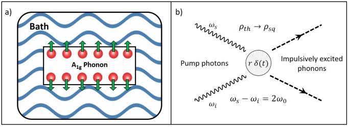
Figure 1: (a) Sketch of the system: a Raman phonon, frequency $\omega_{0}$, in a bath. (b) A pump-induced impulsive second order Raman process at time $t=0$ squeezing the phonon’s thermal density matrix $\rho_{th}\rightarrow\rho_{sq}$, with $r$ the squeeze parameter. $\omega_{i}$ ($\omega_{s}$) is incident (scattered) pump photon frequency.

The purpose of the current work is twofold. (i) First, to bring into question the above state of the art that relates $2\omega_{0}$ noise oscillation with squeezing. As we show below, there are out of equilibrium mechanisms that do not involve phonon squeezing and yet which lead to $N_{X}(t)\sim\sin(2\omega_{0}t)$. Thus, by itself, such a signal is not sufficient to conclude having phonon squeezed state. In fact, the main ingredient for $2\omega_{0}$ oscillatory signal appear to be the breaking of time translation symmetry by a quench, which may or may not involve squeezing the phonon. (ii) Second, we identify a more reliable method to detect a squeezed phonon state, which involves both time- and frequency- resolved Raman measurement.

II Model

We consider a Brillouin zone center Raman-active optical phonon with dimensionless canonical variables $(X,P)$, coupled to a spinless fermionic bath with dispersion $\epsilon_{{\bf k}}$, momentum ${\bf k}$, and described by operators $(c^{\dagger}_{{\bf k}},c_{{\bf k}})$ [see Fig. 1(a)]. The equilibrium Hamiltonian is

$$\mathcal{H}=\frac{\hbar\omega_{0}}{2}(X^{2}+P^{2})+\sum_{{\bf k}}\left(\epsilon_{{\bf k}}+\frac{VX}{\sqrt{2N}}F_{{\bf k}}\right)c^{\dagger}_{{\bf k}}c_{{\bf k}}.$$ (1)

$V$ is the phonon-bath interaction energy, assumed to be small enough such that it can be treated perturbatively. $F_{{\bf k}}$ is a form factor that reflects the point group symmetry of the phonon, and $N$ is the total number of bath variables. The role of the bath is simply to provide a finite inverse lifetime $\gamma$ to the phonon, and to define a temperature $T$ for the system. We assume $\omega_{0}>\gamma$.

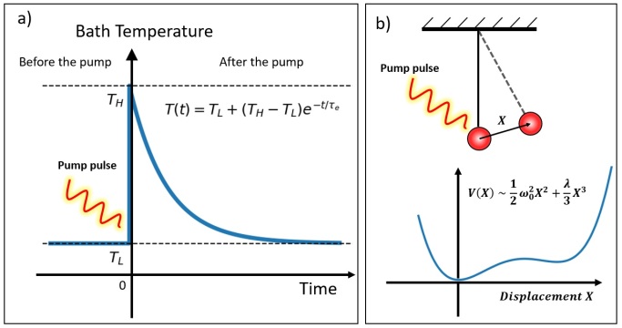
Figure 2: Two out-of-equilibrium processes that do not involve creating a squeezed phonon with density matrix $\rho_{sq}$, but whose noise signal $N_{X}(t)\sim\sin(2\omega_{0}t)$ has the same oscillatory component as the squeezed case. (a) The bath temperature is quenched by the pump. (b) A phonon, with a cubic anharmonic potential, is excited coherently by the pump.

The system is subjected to a laser pump pulse of femtosecond duration at time $t=0$, and we consider three different possible outcomes of this out-of-equilibrium perturbation that can manifest at a picosecond scale. (i) First, we consider the outcome that the phonon is squeezed by the pump via an impulsive resonant second order Raman scattering process which leads to the generation/absorption of two phonon quanta [see Fig. 1(b)]. The perturbation is described by $\delta\mathcal{H}_{(i)}=r\delta(t)(X^{2}-P^{2})/2$, where $r$ is the dimensionless squeezing factor. (ii) Second, we consider the outcome that the pump leads to heating of the bath, such that the bath temperature becomes time dependent. We model the thermal quench as $T(t)=T_{L}$ for $t<0$, and $T(t)=T_{L}+(T_{H}-T_{L})e^{-t/\tau_{e}}$, with $T_{H}\geq T_{L}$ [see Fig. 2(a)]. Here $\tau_{e}$ is the thermal relaxation timescale of the bath. In this case the bath density matrix is perturbed. (iii) Third, we consider the outcome that the phonon, assuming it has a symmetry-allowed cubic anharmonic potential, is coherently excited by the pump pulse [see Fig. 2(b)]. The generation mechanism of the coherent phonon, either via impulsive Raman scattering [15] or via displacive excitation [14], is unimportant here. This outcome is described by $\delta\mathcal{H}_{(iii)}=\hbar\omega_{0}f(t)X+\lambda X^{3}/3$, where $f(t)$ is the time-dependent force that excites the phonon coherently, and $\lambda$ is the energy scale of the cubic anharmonic potential. Importantly, such a cubic anharmonicity is relevant in most systems that have been studied to date in the context of squeezing. These include fully symmetric $A_{g}$-phonons in all systems, as well as $E_{g}$-phonons in bismuth and $\alpha$-quartz with $D_{3}$ point group. Note, for low enough pump fluence, the signatures of all these three outcomes depend linearly on the fluence.

Our goal is to study the fluctuation/noise $N_{X}(t)$ generated for each of the above three outcomes separately. We work using the Keldysh formalism, where the phonon coordinate is defined on a two-branch real-time contour, $X_{\pm}(t)$. We integrate out the bath variables, treating the coupling $V$ to second order, and write the phonon action in the more physical classical and quantum basis $X_{cl/q}=\left(X_{+}\pm X_{-}\right)/\sqrt{2}$ as [36, 37]

$$S[X]=\int_{-\infty}^{\infty}dt^{\prime}\int_{-\infty}^{\infty}dt\;X^{T}(t^{\prime})\hat{D}_{\rm inv}(t^{\prime},t)X(t),$$ (2)

where $X^{T}(t)\equiv(X_{\rm cl}(t),X_{\rm q}(t))$, and the matrix

$$\hat{D}_{\rm inv}(t^{\prime},t)\equiv\begin{bmatrix}0&D_{A}^{-1}(t^{\prime},t)\\ D_{R}^{-1}(t^{\prime},t)&-\Pi_{K}(t^{\prime},t)\end{bmatrix}.$$

$D_{R/A}^{-1}(t^{\prime},t)=D_{0,R/A}^{-1}(t^{\prime},t)-\Pi_{R/A}(t^{\prime},t)$ are the inverse retarded(advanced) phonon propagators and $D_{0,R/A}^{-1}(t^{\prime},t)$ are those of a free phonon. The self-energy contributions $\Pi_{R/A/K}(t^{\prime},t)$ from the fermionic bath are given by

$$\Pi_{R}(t^{\prime},t)=\Pi_{{\rm cl},{\rm q}}(t^{\prime},t)\equiv-iV^{2}\sum_{{\bf k}}F_{{\bf k}}^{2}\langle n_{{\bf k},{\rm cl}}(t^{\prime})n_{{\bf k},{\rm q}}(t)\rangle_{S_{\rm b}^{0}},$$

$\Pi_{A}(t^{\prime},t)=\Pi_{{\rm q},{\rm cl}}(t^{\prime},t)$, and $\Pi_{K}(t^{\prime},t)=\Pi_{{\rm cl},{\rm cl}}(t^{\prime},t)$. $S_{\rm b}^{0}$ is the action of the bare bath, and $n_{{\bf k},{\rm cl/q}}\equiv(c^{\dagger}_{{\bf k},{\rm cl}}c_{{\bf k},{\rm cl/q}}+c^{\dagger}_{{\bf k},{\rm q}}c_{{\bf k},{\rm q/cl}})/\sqrt{2}$. From Eq. (2) we get

$$\langle X_{\rm cl}(t)^{2}\rangle_{S[X]}=i\int_{-\infty}^{\infty}dt^{\prime\prime}dt^{\prime}D_{R}(t,t^{\prime\prime})D_{R}(t,t^{\prime})\Pi_{K}(t^{\prime\prime},t^{\prime}),$$ (3)

which is the out-of-equilibrium generalization of the fluctuation-dissipation relation. Our task is to obtain $D_{R}(t^{\prime},t)$ and $\Pi_{K}(t^{\prime},t)$, and from these to calculate the noise $N_{X}(t)$ for the above three cases.

III Results

Our main results are as follows. (1) We show that for all the three cases the noise signal has a $2\omega_{0}$-oscillatory component with $N_{X}(t)\sim\sin(2\omega_{0}t)$. Yet, only in case (i) the signal is from a phonon squeezed state. Thus, a $2\omega_{0}$-oscillatory noise signal is not sufficient to conclude whether the phonon is in the squeezed state $\rho_{sq}$ or not. (2) By comparing the phonon spectral function for the three cases, we obtain a reliable method to detect a squeezed phonon state $\rho_{sq}$ which involves time-and frequency-resolved Raman measurement.

III.1 Case (i): Noise from squeezing

As the bath itself is in equilibrium with temperature $T$, $\Pi_{K}(t^{\prime},t)$ is a function of $(t^{\prime}-t)$, and its Fourier transform $\Pi_{K,{\rm eq}}(\omega)$ satisfies standard fluctuation-dissipation theorem $\Pi_{K,{\rm eq}}(\omega)=[\Pi_{R,{\rm eq}}(\omega)-\Pi_{A,{\rm eq}}(\omega)]\coth[\omega/(2T)].$ As we are interested in the long-time dynamics of the phonon, it is enough to expand $\Pi_{R,{\rm eq}}(\omega)$ in frequency. Since charge excitations are gapless in a good fermionic bath, we get ${\rm Im}\Pi_{R,{\rm eq}}(\omega)\approx-\omega\gamma/\omega_{0}$, and $\Pi_{K,{\rm eq}}(\omega)\approx-2i\omega\gamma\coth[\omega/(2T)]/\omega_{0}.$ Next, due to $\delta\mathcal{H}_{(i)}$ the squeezing perturbation, $D_{R}(t^{\prime},t)$ satisfies

$$\left[h(t)\partial_{t}^{2}+\dot{h}(t)\partial_{t}+2\gamma\partial_{t}+r\omega_{0}\delta(t)+\omega_{0}^{2}\right]D_{R}(t^{\prime},t)$$

$$=-2\omega_{0}\delta(t^{\prime}-t),$$

where $h(t)\equiv\omega_{0}/[\omega_{0}-r\delta(t)]$, $\dot{h}(t)=\partial_{t}h(t)$, while $\gamma$ plays the role of phonon damping induced by the fermionic bath. The solution of the above equation with the initial conditions $D_{R}(t^{+},t)=0$ and $\partial_{t}D_{R}(t^{+},t)=-2\omega_{0}$ is described in detail in Appendix A. Here we simply quote the final answer. Before that, for convenience, we introduce the notation

$$\mathcal{F}_{T}[f(x_{1},x_{2},\cdots);x_{i};k_{i}]\equiv\int_{-\infty}^{\infty}dx_{i}e^{ik_{i}x_{i}}f(x_{1},x_{2},\cdots).$$

In terms of $\Delta_{R}(t,\omega)\equiv\mathcal{F}_{T}[D_{R}(t,t-\tau);\tau;\omega]$ we get

$$\Delta_{R}(t,\omega)=\left[1+\frac{i}{2\omega_{0}}\theta(t)K(t,\omega)e^{i\omega t-\gamma t}\right]D_{R,{\rm eq}}(\omega),$$ (4)

where $D_{R,{\rm eq}}(\omega)\equiv 2\omega_{0}/[\omega^{2}+2i\gamma\omega-\omega_{0}^{2}]$ is the equilibrium propagator, and $K(t,\omega)\equiv A(t)(\omega-\omega_{0}+i\gamma)e^{i\omega_{0}t}+\bar{A}(t)(\omega+\omega_{0}+i\gamma)e^{-i\omega_{0}t}$. The function $A(t)\equiv\sinh r\cos(2\omega_{0}t)+i[\cosh r-\sinh r\sin(2\omega_{0}t)-1]$ has information about squeezing. Re-expressing Eq. (3) in terms of $\Delta_{R}(t,\omega)$ and $\Pi_{K,{\rm eq}}(\omega)$ we get [38]

$$N_{X}(t)=\frac{1}{2}e^{-2\gamma t}\sinh 2r[\tanh r-\sin(2\omega_{0}t)]\coth\frac{\omega_{0}}{2T}.$$ (5)

Thus, $N_{X}(t)$ has a $2\omega_{0}$ oscillatory component.

III.2 Case (ii): Noise from thermal quench of bath

Here we assume that the effect of the pump on the bath can be encoded by a slowly varying effective temperature, $T(s)=T_{L}+\theta(s)(T_{H}-T_{L})e^{-s/\tau_{e}}$, for time scales much longer than those relevant for the internal electronic dynamics. Thus, we disregard the processes by which the bath itself thermalises to an effective time-dependent temperature, and we study the consequences of such a pseudo-equilibrium environment on the phonon noise.

A first effect of the pseudo-equilibrium is that the Keldysh self-energy $\Pi_{K}(t^{\prime},t)$, sensitive to the occupation of the bath modes, loses time-translational invariance and acquires a dependence on the average time $s\equiv(t^{\prime}+t)/2$ via the temporally varying temperature. It is convenient to define $\Pi_{K}(s,\omega)\equiv\mathcal{F}_{T}[\Pi_{K}(s+\tau/2,s-\tau/2);\tau;\omega]$. We expect that $\Pi_{K}(s,\omega)$, in analogy with $\Pi_{K,{\rm eq}}(\omega)$, satisfies the fluctuation-dissipation relation with the time-dependent temperature $T(s)$. This implies that $\Pi_{K}(s,\omega)\approx-2i\omega\gamma\coth[\omega/(2T(s))]/\omega_{0}.$ In principle, the retarded phonon propagator $D_{R}(t^{\prime},t)$ also acquires $s$-dependence through the temperature dependence of damping $\gamma(s)$. However, to leading order in the temperature quench $(T_{H}-T_{L})$ this slow variation can be ignored, and one can use the equilibrium form $D_{R,{\rm eq}}(\omega)$. Note that, the above simplification does not affect the final conclusion qualitatively.

From the above considerations, it is simple to evaluate the fluctuations in terms of $\langle X_{\rm cl}(\Omega)^{2}\rangle_{S[X]}\equiv\mathcal{F}_{T}[\langle X_{\rm cl}(t)^{2}\rangle_{S[X]};t;\Omega]$ from the relation

$$\langle X_{\rm cl}(\Omega)^{2}\rangle_{S[X]} =\frac{i}{4\pi}\int_{-\infty}^{\infty}ds\int_{-\infty}^{\infty}d\omega D_{R,{\rm eq}}(\omega+\Omega/2)$$

$$\times D^{\ast}_{R,{\rm eq}}(\omega-\Omega/2)\Pi_{K}(s,\omega)e^{i\Omega s}.$$

We assume that $\gamma$ is the lowest energy scale and, in particular, $\gamma\ll T_{L}$. Then,

$$\langle X_{\rm cl}(\Omega\sim\pm 2\omega_{0})^{2}\rangle_{S[X]}\propto\frac{1}{z_{1}z_{2}}\int_{-\infty}^{\infty}dse^{i\Omega s}\Pi_{K}(s,\omega\rightarrow 0),$$

where $z_{1,2}\equiv\Omega/2\pm\omega_{0}+i\gamma$. This implies that $\langle X_{\rm cl}(\Omega)^{2}\rangle_{S[X]}$ has poles at $\Omega=\pm 2\omega_{0}$, which in the time domain translate as $\sin(2\omega_{0}t)$ oscillations. Note, the origin of the these poles is an equilibrium property of a damped oscillator. However, in equilibrium time translation symmetry ensures that $\Pi_{K}(s,\omega)$ does not depend upon the average time $s$. In such a case the $s$-integral above gives $\delta(\Omega)$ and, therefore, in equilibrium the finite-$\Omega$ poles are “inaccessible”. Keeping the $s$-dependence of $\Pi_{K}(s,\omega)$ we get

$$N_{X}(t)=\frac{-\gamma(T_{H}-T_{L})}{2\omega_{0}^{2}}e^{-2\gamma t}\sin(2\omega_{0}t)+\ldots,$$ (6)

where the ellipsis imply non-oscillatory contributions. Thus, we demonstrate that $N_{X}(t)$ can have $2\omega_{0}$ oscillatory signal simply due to pump induced thermal quench of the bath. In fact, any out-of-equilibrium perturbation of the bath that breaks time translation symmetry will lead to a $2\omega_{0}$ oscillatory noise signal.

III.3 Case (iii): Noise from phonon with cubic anharmonicity coherently excited

This is relevant for $A_{g}$ phonons in all systems, and also for $E_{g}$ phonons in $D_{3}$ symmetric systems such as $\alpha$-quartz and bismuth. The pump leads to $\langle X_{\rm cl}(t)\rangle_{S[X]}\equiv u(t)\neq 0$, where $u(t)$ describes the coherent excitation. To study the fluctuations around the average we expand the action in terms of $\delta X\equiv X-u(t)$. This gives Eq. (2) with $X_{\rm cl}$ replaced by $\delta X_{\rm cl}$, and with the propagator $D_{R}(t^{\prime},t)$ satisfying the equation

$$\left[\partial_{t}^{2}+2\gamma\partial_{t}+\omega_{0}^{2}+4\lambda\omega_{0}u(t)\right]D_{R}(t^{\prime},t)=-2\omega_{0}\delta(t^{\prime}-t).$$

In the above the crucial ingredient is the $\lambda u(t)$ term which acts as a time dependent potential for the fluctuations. We assume $\lambda/\omega_{0}\ll 1$, such that it is sufficient to solve the above equation to linear order in $\lambda$. We expand $D_{R}(t^{\prime},t)=D_{R,{\rm eq}}(t^{\prime}-t)+\lambda D_{R,1}(t^{\prime},t)$ with

$$D_{R,1}(t^{\prime},t)=2\int_{-\infty}^{\infty}dsD_{R,{\rm eq}}(t^{\prime}-s)u(s)D_{R,{\rm eq}}(s-t).$$

On the other hand the bath is in equilibrium with temperature $T$, and therefore the Keldysh self-energy is the one in equilibrium $\Pi_{K,{\rm eq}}(\omega)$. Ignoring the equilibrium contribution to noise we get

$$N_{X}(t)_{\rm non-eq}$$

$$=-i\lambda\int_{-\infty}^{\infty}dsds^{\prime}D_{R,{\rm eq}}(t-s)D_{R,1}(t,s^{\prime})\Pi_{K,{\rm eq}}(s-s^{\prime})$$

$$=4\lambda\coth(\frac{\omega_{0}}{2T})\int_{0}^{t}ds\;u(s)\sin[2\omega_{0}(t-s)]e^{-2\gamma(t-s)}.$$

In the last line the $s$-integral starts from $s>0$ because the coherent excitation is triggered by the pump at $s=0$. This element of time translation symmetry breaking is crucial. Irrespective of the details of the coherent motion $u(s)$, it is clear from the above that there is an oscillatory $2\omega_{0}$-signal in the noise. The precise form of $N_{X}(t)$ depend on the force $f(s)$, which determines $u(s)$. An impulsive excitation leads to $u(s)=u_{0}\sin(\omega_{0}s)e^{-\gamma s}$, and

$$N_{X}(t)_{\rm non-eq}=-\frac{4\lambda u_{0}\coth[\omega_{0}/(2T)]}{3\omega_{0}}e^{-2\gamma t}\sin(2\omega_{0}t)+\ldots,$$ (7)

where the ellipsis imply terms not relevant for the current discussion. For a displacive coherent excitation the sine signal is replaced by a cosine, which reflects the property of coherent phonons that the phase of the oscillation is determined by the generation mechanism [14, 15, 16]. Thus, as in case (ii), we obtain oscillatory $2\omega_{0}$- noise signal without having created the density matrix $\rho_{sq}$. However, in contrast to case (ii) which involves only incoherent excitations, in (iii) the $2\omega_{0}$ signal is built out of a coherent excitation at $\omega_{0}$. Consequently, the latter is analogous to higher harmonic generation.

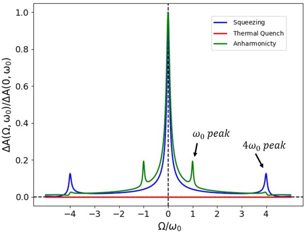
Figure 3: The time dependence of the spectral function peak $\Delta A(t,\omega_{0})\equiv A(t,\omega_{0})-A(0,\omega_{0})$ (see Eq. (8) for definition) and its Fourier transform $\Delta A(\Omega,\omega_{0})$ have distinct signatures for the three cases studied here. A distinguishing feature of squeezing is a single peak in $|\Delta A(\Omega,\omega_{0})|$ at $\Omega=4\omega_{0}$.

III.4 Reliable signature of squeezed phonon

Next, we identify a measurable quantity that can distinguish a squeezed phonon, i.e., case (i) from (ii) and (iii). Since the noise $N_{X}(t)$, which is a time resolved but frequency integrated quantity, has the same oscillatory property for the three situations, a promising direction is to look for a quantity which is both time and frequency resolved. With this intuition we define the time- and frequency- resolved spectral function

$$A(t,\omega)\equiv{\rm Im}D_{R}(t,\omega),$$ (8)

where $D_{R}(t,\omega)\equiv\mathcal{F}_{T}[D_{R}(t+\tau/2,t-\tau/2);\tau;\omega]$ is the Wigner transform of the two-time retarded propagator. Note, $D_{R}(t,\omega)$ is to be distinguished from $\Delta_{R}(t,\omega)$ defined earlier. In equilibrium, $A(t,\omega)$ is $t$-independent and is peaked at $\omega=\pm\omega_{0}$. Thus, $A(t,\omega_{0})$ describes how the spectral peak varies with time $t$ after the pump.

We find that, indeed, the $t$-dependencies of $A(t,\omega_{0})$ for the three cases are distinct, since the phonon propagator $D_{R}(t,\omega)$ in the three cases are quite different (for details see Appendix B). In case (i) squeezing leads to $A(t,\omega_{0})$ to oscillate with frequency 4$\omega_{0}$ as a function of $t$ for the following reason. Since squeezing involves excitation of two phonon quanta, $D_{R}(t+\tau/2,t-\tau/2)\sim\cos(2\omega_{0}t)\theta(\tau-2t)$. The constraint $\tau\geq 2t$ is crucial, and follows from the fact that squeezing is an impulsive process occurring at time zero [see Fig. 1(b)], and so the two time arguments in $D_{R}(t+\tau/2,t-\tau/2)$ must have opposite signs (see Eq. (27) in the Appendix). Next, the Wigner transform involves multiplication of the phase $\exp(i\omega\tau)$, and therefore, imposing the constraint leads, via phase accumulation, to $A(t,\omega_{0})\sim\cos(4\omega_{0}t+\phi)$, where $\phi$ is a phase that depends on details. Thus, the $4\omega_{0}$ oscillation is a consequence of impulsive excitation of two phonon quanta, which is the hallmark of squeezing. In case (ii) $A(t,\omega_{0})$ is practically $t$-independent, since the weak $t$-dependence of the phonon self-energy induced by the electronic bath can be disregarded. In case (iii) $A(t,\omega_{0})$ has oscillations at frequencies 4$\omega_{0}$, but also at $\omega_{0}$. The latter is due to the fact that in this scenario the phonon is excited coherently. This exemplifies that processes involving higher harmonic generation invariably will have a signature at a frequency lower than $4\omega_{0}$, and thus, they can be distinguished from squeezing.

These three distinct $t$-dependencies can be conveniently expressed in terms of $\Delta A(\Omega,\omega_{0})\equiv\mathcal{F}_{T}[\Delta A(t,\omega_{0});t;\Omega]$, where $\Delta A(t,\omega_{0})\equiv A(t,\omega_{0})-A(0,\omega_{0})$ is the time dependent part of the spectral function peak. Thus, as shown in Fig. 3, a distinguishing feature of squeezing is a single peak in $|\Delta A(\Omega,\omega_{0})|$ at $\Omega=4\omega_{0}$.

Finally, we discuss how the time dependent spectral function $A(t,\omega)$ can be measured. In equilibrium this is standard since the Raman scattering cross-section is proportional to the correlation function, and from which the spectral function can be deduced using fluctuation-dissipation relation. The issue is nontrivial in an out of equilibrium situation since the standard fluctuation-dissipation relation is not valid. However, we can generalize the relation in the following manner. According to the theory of time and frequency resolved Raman spectroscopy the scattering intensity $I(t,\omega)\propto D^{>}(t,\omega)$, where $D^{>}(t,\omega)$ is the Wigner transform of the two-time greater function [39, 40]. Then, from standard Keldysh theory it follows that $I(t,\omega)-I(t,-\omega)\propto A(t,\omega)$ (see Appendix C). In other words, the time dependent spectral function can be extracted from the difference of the Stokes and anti-Stokes Raman intensities. In practice, the probe cycle will require two pulses, one which is time-resolved and a second which is frequency-resolved [41, 42].

IV Conclusion

To summarize, we studied the fluctuations of a phonon coupled to a bath in a pump-probe setup. We argued that the noise or the variance associated with the atomic displacement oscillates at twice the phonon frequency $\omega_{0}$, i.e. $N_{X}(t)\equiv\langle X(t)^{2}\rangle-\langle X(t)\rangle^{2}\sim\sin(2\omega_{0}t)$, due to pump-induced breaking of time translation symmetry. Thus, such oscillations cannot be taken as proof of having prepared the phonon in a squeezed state with density matrix $\rho_{sq}$. A reliable way to identify squeezed phonons involve a study of the time-dependent spectral function of the phonon which can be achieved by a time and frequency resolved Raman measurement.

Appendix A Retarded Green’s function of a squeezed phonon

The retarded phonon Green’s function of a squeezed phonon coupled to a thermal bath satisfies the equation of motion

$$\frac{1}{2\omega_{0}}\left(h(t)\partial_{t}^{2}+\dot{h}(t)\partial_{t}+2\gamma\partial_{t}+\omega_{0}^{2}+g(t)\omega_{0}\right)D_{R}(t,t^{\prime})$$

$$=\delta(t-t^{\prime}),$$ (9)

where $h(t)=\omega_{0}/(\omega_{0}-rg(t))$, and $g(t)$ describes the envelope of the pump-pulse. We assume that the width of the pump-pulse is the smallest time scale of the problem, and hence, that it can be well approximated by a Dirac distribution. It is, however, uncomfortable to deal with the non-analyticity of the Dirac distribution in path integrals. Indeed, for a delta shaped pump pulse centered at time $t=0$, the displacement $X_{cl/q}(t)$ and momentum $P_{cl/q}(t)(t)$ fields are not well defined at initial time $t=0$. In practice, however, the shape of a physical pump-pulse is a smooth function with a finite width $\tau_{p}$, and the approximation with a Dirac distribution is just a practical mathematical description. Therefore, to avoid complication, we solve the problem for a general pulse with a smooth envelope $g(t)$ centered at time $t=0$ and a finite width $\tau_{p}$, and only take the limit $\tau_{p}\rightarrow 0$ for which $g(t)\rightarrow r\delta{(t)}$ at the end of the calculation.

The Dirac delta function $\delta(t-t^{\prime})$ is vanishing for $t\neq t^{\prime}$, hence, for time $t\neq t^{\prime}$ the Green’s function satisfies the homogeneous equation

$$\bigg{(}h(t)\partial_{t}^{2}+h^{\prime}(t)\partial_{t}+2\gamma\partial_{t}+\omega_{0}^{2}+g(t)\omega_{0}\bigg{)}D_{R}(t,t^{\prime})=0.$$ (10)

The retarded Green’s function has a causal structure, i.e. it vanishes for $t<t^{\prime}$, and satisfies a second order differential equation which boundary condition are given by the definition of the retarded Green’s function at equal time

$$D_{R}(t^{+},t)=-i\langle\left[\hat{X}(t^{+}),\hat{X}(t)\right]\rangle=0,$$ (11)

and the jump condition imposed by the delta function

$$\partial_{t}D_{R}(t^{+},t)=-2\omega_{0},$$ (12)

where $t^{+}=t+0^{+}$.

We replace the equation of the retarded Green’s function Eq. (A) by a set of two coupled first order equations and write

$$\partial_{t}D_{R}(t,s) =\left[\omega_{0}-g(t)\right]K(t,s),$$ (13a)

$$\partial_{t}K(t,s) =-\left[\omega_{0}+g(t)\right]D_{R}(t,s)-2\frac{\gamma}{\omega_{0}}\partial_{t}D_{R}(t,s),$$ (13b)

where $K(t,s)$ is a function that we introduce as a mathematical tool. Notice that for $g(t)=0$, the equation of the retarded Green’s function Eq. (13) is that of a damped harmonic oscillator. Therefore, we propose the following ansatz for the solution

$$D_{R}(t,s) =X_{0}(t,s)\cos(\Omega t)e^{-\gamma t}$$

$$+\frac{1}{\Omega}\left[\omega_{0}P_{0}(t,s)+\gamma X_{0}(t,s)\right]\sin(\Omega t)e^{-\gamma t},$$ (14a)

$$K(t,s) =P_{0}(t,s)\cos(\Omega t)e^{-\gamma t}$$

$$-\frac{1}{\Omega}\left[\omega_{0}X_{0}(t,s)+\gamma P_{0}(t,s)\right]\sin(\Omega t)e^{-\gamma t},$$ (14b)

where $\Omega^{2}=\omega_{0}^{2}-\gamma^{2}$. This form of the solution ensures that for constant $X_{0}(t,s)$ and $P_{0}(t,s)$, the functions $D_{R}(t,s)$ and $K(t,s)$ satisfy the equation of motion of a damped harmonic oscillator. The fact that the phonon is a well defined excitation implies that $\gamma\ll\omega_{0}$. Thus, we write the equations of motion for $X_{0}(t,s)$ and $P_{0}(t,s)$ in this limit and find that

$$\begin{split}\begin{bmatrix}\partial_{t}X_{0}(t,s)\\ \partial_{t}P_{0}(t,s)\end{bmatrix}&=-g(t)\begin{bmatrix}-\sin{\left(2\Omega t\right)}&\cos{\left(2\Omega t\right)}\\ \cos{\left(2\Omega t\right)}&\sin{\left(2\Omega t\right)}\end{bmatrix}\begin{bmatrix}X_{0}(t,s)\\ P_{0}(t,s)\end{bmatrix}.\end{split}$$ (15)

We take the limit where the width of the pump-pulse goes to zero $\tau_{p}\rightarrow 0$ and recover the Dirac delta function $g(t)\rightarrow r\delta(t)$. Using the properties of the Dirac distribution, we have that

$$\sin(\Omega t)g(t) =\sin(0)g(t)=0,$$ (16a)

$$\cos(\Omega t)g(t) =\cos(0)g(t)=g(t),$$ (16b)

hence Eq. (15) further simplifies, and we obtain

$$\begin{split}\begin{bmatrix}\partial_{t}X_{0}(t,s)\\ \partial_{t}P_{0}(t,s)\end{bmatrix}&=-g(t)\begin{bmatrix}0&1\\ 1&0\end{bmatrix}\begin{bmatrix}X_{0}(t,s)\\ P_{0}(t,s)\end{bmatrix}.\end{split}$$ (17)

The solution of this equation of motion is straightforward, and after some algebraic manipulations we find that

$$X_{0}(t,s) =\mathrm{ch}[F(t,s)]K_{1}(s)-\mathrm{sh}[F(t,s)]K_{2}(s),$$ (18a)

$$P_{0}(t,s) =\mathrm{ch}[F(t,s)]K_{2}(s)-\mathrm{sh}[F(t,s)]K_{1}(s),$$ (18b)

with

$$F(t,s)=\int_{s}^{t}g(t^{\prime})dt^{\prime},$$ (19)

where $\mathrm{ch}(x)$ and $\mathrm{sh}(x)$ denote the cosine and sine hyperbolic functions, respectively. $K_{1}(s)$ and $K_{2}(s)$ are arbitrary functions independent of time $t$, that are to be calculated using the boundary conditions, see Eq. (11) and Eq. (12). We take the limit $\gamma\ll\omega_{0}$, and write the propagator in a more convenient form

$$D_{R}(t,s) =\left(\mathrm{ch}[F(t,s)]\sin{\left[\Omega(t-s)-\phi(s)\right]}\right.$$

$$-\left.\mathrm{sh}[F(t,s)]\cos{\left[\Omega(t+s)+\phi(s)\right]}\right)A(s)e^{-\gamma(t-s)},$$ (20)

where we replaced the functions K1(s) and K2(s) by two other unknown functions $A(s)$ and $\phi(s)$ defined as

$$K_{1}(s) =-A(s)\sin{\big{(}\Omega s+\phi(s)\big{)}}e^{\gamma s},$$ (21a)

$$K_{2}(s) =A(s)\cos{\big{(}\Omega s+\phi(s)\big{)}}e^{\gamma s}.$$ (21b)

The functions $A(s)$ and $\phi(s)$ can be evaluated using the boundary conditions. We use the continuity condition Eq. (11) of the retarded Green’s function

$$\sin{\left[-\phi(t)\right]}A(t)=0,\\$$ (22)

together with the jump condition Eq. (11) at time $t\neq 0$

$$\begin{split}A(t)\bigg{(}\Omega-\delta(t)\cos{(2\Omega t)}\bigg{)}=-2\omega_{0},\end{split}$$ (23)

and find that

$$\phi(s) =0,$$ (24a)

$$A(s) =-2,$$ (24b)

which gives for the retarded Green’s function

$$D_{R}(t,s) =-2\theta(t-s)\left(\mathrm{ch}[F(t,s)]\sin{\left[\Omega(t-s)\right]}\right.$$

$$-\left.\mathrm{sh}[F(t,s)]\cos{\left[\Omega(t+s)\right]}\right)e^{-\gamma(t-s)}.$$ (25)

In the limit of delta shaped pump-pulse $g(t)=r\delta(t)$, we have that

$$F(t,s) =r\int^{t}_{s}\delta(t^{\prime})dt^{\prime}=r, \mathrm{sign}(t)\neq\mathrm{sign}(s)$$ (26a)

$$F(t,s) =r\int^{t}_{s}\delta(t^{\prime})dt^{\prime}=0, \mathrm{sign}(t)=\mathrm{sign}(s)$$ (26b)

with $\mathrm{sign}(t)$ the sign function. Thus, the retarded phonon Green’s function is defined piece-wise and reads

$$D_{R}(t,s)=\ \begin{cases}D^{R}_{eq}(t,s),&\qquad\rm{sign}(t)=\rm{sign}(s),\\ D^{R}_{sq}(t,s),&\qquad\rm{sign}(t)\neq\rm{sign}(s),\end{cases}$$ (27)

with

$$D^{R}_{eq}(t,s) =-2\theta(t-s)e^{-\gamma(t-s)}\sin{\left[\Omega(t-s)\right]},$$ (28a)

$$D^{R}_{sq}(t,s) =-2e^{-\gamma(t-s)}\theta(t-s)\left(\mathrm{ch}(r)\sin{\left[\Omega(t-s)\right]}\right.$$

$$-\left.\mathrm{sh}(r)\cos{\left[\Omega(t+s)\right]}\right),$$ (28b)

where $D^{R}_{eq}(t,s)$ and $D^{R}_{sq}(t,s)$ stand for the equilibrium and squeezed retarded Green’s function. The fact that the squeezed propagator is not a function of the the time difference $D^{R}_{sq}(t,s)\neq D^{R}_{sq}(t-s)$ is a consequence of breaking time translational symmetry.

We now evaluate the function $\Delta_{R}(t,\omega)$ discussed in the main text and defined as

$$\Delta_{R}(t,\omega)=\int\Delta_{R}(t,t-\tau)e^{i\omega\tau}d\tau.$$ (29)

In time domain, the phonon propagators $D_{R}(t_{1},t_{2})$ of the squeezed phonon is defined piece-wise, see Eq. (28). Thus, we split the integral Eq. (29) over the two time domains and write

$$\Delta_{R}(t,\omega) =\int\limits_{-\infty}^{\infty}D_{eq}^{R}(t,t-\tau)e^{i\omega\tau}d\tau$$

$$+\int\limits_{t}^{\infty}\left(D_{sq}^{R}(t,t-\tau)-D_{eq}^{R}(t,t-\tau)\right)e^{i\omega\tau}d\tau,$$ (30)

where we added and subtracted $\int_{t}^{\infty}D_{eq}^{R}(t,t-\tau)e^{i\omega\tau}d\tau$ to extend the limits of the first integral to $+\infty$. The first term of the integral is the equilibrium contribution and is time independent. The second term is the out-of-equilibrium contribution to the retarded propagator $\Delta_{R}(t,\omega)$, and vanishes for a vanishing squeezing parameter $r=0$ or for negative times $t<0$. For positive times after the pump-pulse $t>0$, we have

$$\begin{split}\small&I(t,\omega)\equiv\int_{t}^{\infty}\left(D_{sq}^{R}(t,t-\tau)-D_{eq}^{R}(\tau)\right)e^{i\omega\tau}d\tau\\ &=-2\int_{t}^{\infty}\bigg{(}g_{2}(t)\sin{\left(\Omega\tau\right)}-g_{1}(t)\cos{\left(\Omega\tau\right)}\bigg{)}e^{(i\omega-\gamma)\tau}d\tau,\\ \end{split}$$ (31)

where the complex functions $g_{1}(t)$ and $g_{2}(t)$ are defined as

$$g_{1}(t) =\mathrm{sh}{(r)}\cos{(2\Omega t)},$$ (32a)

$$g_{2}(t) =\mathrm{ch}{(r)}-\mathrm{sh}{(r)}\sin{(2\Omega t)}-1,$$ (32b)

with $\Omega=\sqrt{\omega_{0}^{2}-\gamma^{2}}$. We define the complex function $A(t)=g_{1}(t)+ig_{2}(t)$ and express the non equilibrium part of the retarded Green’s function $I(\omega,t)$ in a compact exponential form

$$\begin{split}I(t,\omega)&=\int_{t}^{\infty}\bigg{(}A(t)e^{i\Omega\tau}+\bar{A}(t)e^{-i\Omega\tau}\bigg{)}e^{(i\omega-\gamma)\tau}d\tau,\\ &=\frac{i}{2\Omega}\left(A(t)\big{(}\omega-\Omega+i\gamma\big{)}e^{i(\omega+\Omega+i\gamma)t}\right.\\ &+\left.\bar{A}(t)\big{(}\omega+\Omega+i\gamma\big{)}e^{i(\omega-\Omega+i\gamma)t}\right)D_{eq}^{R}(\omega),\end{split}$$ (33)

where $D_{eq}^{R}(\omega)$ denotes the equilibrium retarded Green’s function. Henceforth, we take the limit $\gamma\ll\omega_{0}$ for which $\Omega\approx\omega_{0}$, and we write the function $\Delta_{R}(t,\omega)$ as

$$\begin{split}\Delta_{R}(t,\omega)&=\bigg{(}1+\frac{i}{2\omega_{0}}\theta(t)e^{-\gamma t}K(t,\omega)e^{i\omega t}\bigg{)}D_{eq}^{R}(\omega),\end{split}$$ (34)

so that

$$D^{R}_{eq}(\omega) =\frac{2\omega_{0}}{\omega^{2}+2i\gamma\omega-\omega_{0}^{2}},$$ (35a)

$$K(t,\omega) =A(t)\big{(}\omega-\omega_{0}+i\gamma\big{)}e^{i\omega_{0}t}$$

$$+\bar{A}(t)\big{(}\omega+\omega_{0}+i\gamma\big{)}e^{-i\omega_{0}t}.$$ (35b)

This gives Eq. (4) in the main text. The out of equilibrium part of the retarded Green’s function, as defined in Eq. (29), has a $2\omega_{0}$ oscillatory component. This follows from the definition of the function $A(t)$, whose real and imaginary part oscillate as $\cos(2\omega_{0}t)$ and $\sin(2\omega_{0}t)$, respectively.

We insert the Fourier transform of the retarded Green’s function $\Delta_{R}(t,\omega)$ in the expression of the equal time correlation function and write for time $t>0$

$$\begin{split}\langle X^{2}_{cl}(t)\rangle&=\frac{i}{2\pi}\int\limits^{+\infty}_{-\infty}\Delta_{R}(t,\omega)D^{R}(t,-\omega)\Pi^{K}(\omega)d\omega,\\ &=\frac{1}{2\pi}\int\limits^{+\infty}_{-\infty}\bigg{(}1-y(\omega,t)\bigg{)}D_{eq}^{K}(\omega)d\omega,\\ \end{split}$$ (36)

where $y(\omega,t)$ is the non equilibrium part of the Keldysh Green’s function and is given by

$$y(\omega,t) \equiv\frac{1}{4\omega_{0}^{2}}e^{-2\gamma t}K(t,\omega)K(t,-\omega)$$

$$-\frac{i}{2\omega_{0}}e^{-\gamma t}\bigg{(}K(t,-\omega)e^{-i\omega t}+K(t,\omega)e^{i\omega t}\bigg{)}.$$ (37)

We recall that the equilibrium Keldysh Green’s function is given by

$$\begin{split}D^{K}_{eq}(\omega)&=\frac{8\gamma\omega_{0}\omega\coth{\left[\omega/2T\right]}}{\left(\left[\omega-\omega_{0}\right]^{2}+\gamma^{2}\right)\left(\left[\omega+\omega_{0}\right]^{2}+\gamma^{2}\right)}\\ &=\frac{2\gamma\coth{\left[\omega/2T\right]}}{(\omega-\omega_{0})^{2}+\gamma^{2}}-\frac{2\gamma\coth{\left[\omega/2T\right]}}{(\omega+\omega_{0})^{2}+\gamma^{2}},\end{split}$$ (38)

where we see that it is peaked at $\omega=\pm\omega_{0}$ with a width $\gamma$. Therefore, in the limit where $\gamma\ll\omega_{0}$, the $\coth{\left[\omega/2T\right]}$ is a slow function of frequency and the Keldysh Green’s function can be approximated by

$$\begin{split}D^{K}_{eq}(\omega)&\approx\frac{2\gamma\coth{\left[\omega_{0}/2T\right]}}{(\omega-\omega_{0})^{2}+\gamma^{2}}+\frac{2\gamma\coth{\left[\omega_{0}/2T\right]}}{(\omega+\omega_{0})^{2}+\gamma^{2}},\end{split}$$ (39)

where we used $\coth{\left[-\omega_{0}/2T\right]}=-\coth{\left[\omega_{0}/2T\right]}$. We replace in the expression of the equal time correlation function of the classical field and obtain

$$\begin{split}\langle X^{2}_{cl}(t)\rangle&=\frac{2}{\pi}\coth{\left[\omega_{0}/2T\right]}\int\limits^{+\infty}_{-\infty}\frac{\gamma}{(\omega-\omega_{0})^{2}+\gamma^{2}}\\ &\times\left[1-\frac{1}{4\omega_{0}^{2}}e^{-2\gamma t}K(t,\omega)K(t,-\omega)\right.\\ +&\left.\frac{i}{2\omega_{0}}e^{-\gamma t}\bigg{(}K(t,-\omega)e^{-i\omega t}+K(t,\omega)e^{i\omega t}\bigg{)}\right]d\omega.\end{split}$$ (40)

We integrate over the frequency $\omega$ and obtain for the equal time correlation function

$$\begin{split}\langle X^{2}_{cl}(t)\rangle=2\coth{\left[\omega_{0}/2T\right]}&\bigg{[}1-\frac{1}{4\omega_{0}^{2}}e^{-2\gamma t}K(t,\omega_{0}+i\gamma)K(t,-\omega_{0}-i\gamma)\\ &+\frac{i}{2\omega_{0}}e^{-2\gamma t}\bigg{(}K(t,-\omega_{0}-i\gamma)e^{-i\omega_{0}t}+K(t,\omega_{0}+i\gamma)e^{i\omega_{0}t}\bigg{)}\bigg{]}.\\ \end{split}$$ (41)

We take the limit $\gamma\ll\omega_{0}$, and write the correlation function as

$$\begin{split}\langle X^{2}_{cl}(t)\rangle&=2\coth{\left[\omega_{0}/2T\right]}\left[1+e^{-2\gamma t}\bar{A}(t)A(t)\right.\\ &+\left.ie^{-2\gamma t}\left(\bar{A}(t)-A(t)\right)\right].\\ \end{split}$$ (42)

We replace the complex function $A(t)$ by its expression in Eq. (32) and obtain for the variance after simplification

$$\begin{split}\Delta^{2}X(t)&=\coth{\left[\omega_{0}/2T\right]}\left[1+e^{-2\gamma t}\left(\mathrm{ch}(2r)-1\right)\right.\\ &-\left.\mathrm{sh}{(2r)}\sin{\big{(}2\omega_{0}t\big{)}}e^{-2\gamma t}\right],\\ \end{split}$$ (43)

where $r$ is the squeezing parameters. The variance of the atomic displacement oscillates at twice the frequency of the mode $2\omega_{0}$. This is Eq. (5) in the main text.

Appendix B Time resolved spectral function

Here, we discuss the calculation details of the time resolved spectral function defined as

$$\begin{split}A(t,\omega)&\equiv\mathrm{Im}D^{R}(t,\omega),\end{split}$$ (44)

where

$$D^{R}(t,\omega)=\int D^{R}(t+\tau/2,t-\tau/2)e^{i\omega\tau}d\tau,$$ (45)

is the Wigner transform of the retarded Green’s function. We derive the expression of $A(t,\omega)$ in the two scenarios discussed in the main text, namely a squeezed phonon and a phonon, with a cubic anharmonic potential, excited coherently by the pump. We show that the time resolved spectral is qualitatively different for this two case, and can therefore be used to detect phonon squeezed states.

Case (i): Let us first discuss the signature of a squeezed phonon (case $(i)$ of the main text) on the spectral function $A(t,\omega)$. The out of equilibrium part of the Wigner transform is defined as

$$\begin{split}&\Delta D^{R}(t,\omega)\equiv D^{R}(t,\omega)-D_{eq}^{R}(\omega),\\ &=\int\limits_{-\infty}^{+\infty}\bigg{(}D^{R}(t+\tau/2,t-\tau/2)-D_{eq}^{R}(\tau)\bigg{)}e^{i\omega\tau}d\tau,\end{split}$$ (46)

where $D^{R}_{eq}(\omega)$ is the equilibrium retarded Green’s function. In equilibrium, the Wigner transform coincides with its Fourier transform, hence, the retarded Green’s function $D^{R}(t+\tau/2,t-\tau/2)$ of a squeezed phonon is different from equilibrium only for times where $\mathrm{Sign}(t+\tau/2)\neq\mathrm{Sign}(t-\tau/2)$. Therefore, the integral in Eq.(46) is non vanishing only for time $\tau>2t$ where it can be written as

$$\begin{split}\Delta D^{R}(t,\omega)&=\int\limits_{2t}^{\infty}\left[D^{R}_{sq}(t+\frac{\tau}{2},t-\frac{\tau}{2})-D_{eq}^{R}(\tau)\right]e^{i\omega\tau}d\tau,\\ &=-2\big{(}\mathrm{ch}(r)-1\big{)}\int\limits_{2t}^{\infty}\sin(\omega_{0}\tau)e^{-\gamma\tau}e^{i\omega\tau}d\tau\\ &+2\mathrm{sh}(r)\cos(2\omega_{0}t)\int\limits_{2t}^{\infty}e^{-\gamma\tau}e^{i\omega\tau}d\tau.\end{split}$$ (47)

We get

$$\begin{split}&\Delta D^{R}(t,\omega)=+2\mathrm{sh}(r)\cos(2\omega_{0}t)\int\limits_{2t}^{\infty}e^{-\gamma\tau}e^{i\omega\tau}d\tau\\ &+i\big{(}\mathrm{ch}(r)-1\big{)}\int\limits_{2t}^{\infty}\left[e^{i(\omega+\omega_{0}+i\gamma)\tau}-e^{i(\omega-\omega_{0}+i\gamma)\tau}\right]d\tau.\end{split}$$ (48)

We integrate over time $\tau$ and find

$$\begin{split}\Delta D^{R}(t,\omega)=\big{(}1-\mathrm{ch}(r)\big{)}e^{-2\gamma t}\left[\frac{e^{2i(\omega+\omega_{0})t}}{\omega+\omega_{0}+i\gamma}-\frac{e^{2i(\omega-\omega_{0})t}}{\omega-\omega_{0}+i\gamma}\right]+2i\mathrm{sh}(r)\cos(2\omega_{0}t)e^{-2\gamma t}\frac{e^{2i\omega t}}{\omega+i\gamma}.\end{split}$$ (49)

Thus the spectral function $A(t,\omega_{0})$ evaluated at frequency $\omega_{0}$ has a $4\omega_{0}$ oscillatory component in time domain, coming from the first and third terms above.

Case (iii): We now calculate the spectral function of a phonon, with a cubic anharmonic potential, excited coherently by the pump (case $(iii)$ of the main text). The first order correction of the retarded Green’s function, discussed in the main text, is given by

$$D_{R,1}(t,t^{\prime})=2\int D_{R,eq}(t-s)D_{R,eq}(t^{\prime}-s)u(s)ds.$$ (50)

We Wigner transform the retarded Green’s function and write

$$D_{R,1}(t,\omega) =2\int D_{R,eq}(t+\tau/2-s)$$

$$\times D_{R,eq}(t-\tau/2-s)u(s)e^{i\omega\tau}d\tau ds.$$ (51)

For simplicity, we discuss the case of an impulsive stimulation for which the retarded Green’s function and the average atomic displacement $u(t)$ are given by

$$\begin{split}D_{R,eq}(t,t^{\prime})&=-2\theta(t-t^{\prime})\mathrm{sin}\left[\omega_{0}(t-t^{\prime})\right]e^{-\gamma(t-t^{\prime})},\\ u(t)&=\theta(t)Q_{0}\mathrm{sin}\left(\omega_{0}t\right)e^{-\gamma t}=-\frac{Q_{0}}{2}D_{R,eq}(t).\end{split}$$ (52)

where $Q_{0}$ denotes the amplitude of the coherent phonon oscillation. We Fourier transform and obtain

$$D_{R,1}(t,\omega) =\frac{Q_{0}}{2\pi}\int D_{R,eq}(\Omega)D_{R,eq}(\omega-\Omega/2)$$

$$\times D_{R,eq}(\omega+\Omega/2)e^{-i\Omega t}d\Omega,$$ (53)

Finally, we integrate over frequency $\Omega$ we find that

$$D_{R,1}(t,\omega)=Q_{0}ie^{-\gamma t}\left[\frac{4\omega_{0}^{2}e^{-i\omega_{0}t}}{A(\omega,\omega_{0})}-\frac{4\omega_{0}^{2}e^{i\omega_{0}t}}{A(\omega,-\omega_{0})}\right]$$

$$+8Q_{0}ie^{-2\gamma t}\left[\frac{4\omega_{0}^{2}e^{2it(\omega+\omega_{0})}}{B(\omega,\omega_{0})}-\frac{4\omega_{0}^{2}e^{2it(\omega-\omega_{0})}}{B(\omega,-\omega_{0})}\right]$$ (54)

with

$$A(\omega,\omega_{0}) =(\omega-\frac{3\omega_{0}}{2}+i\frac{3\gamma}{2})(\omega+\frac{3\omega_{0}}{2}+i\frac{\gamma}{2})$$

$$\times(\omega+\frac{\omega_{0}}{2}+i\frac{3\gamma}{2})(\omega-\frac{\omega_{0}}{2}+i\frac{\gamma}{2}),$$ (55a)

$$B(\omega,\omega_{0}) =(4\omega+4\omega_{0}+4i\gamma)(4\omega+4i\gamma)$$

$$\times(2\omega+3\omega_{0}+i\gamma)(2\omega+\omega_{0}+i\gamma).$$ (55b)

From the above expression, we see that the spectral function $A(t,\omega_{0})$ evaluated at frequency $\omega_{0}$ has both a $4\omega_{0}$ (third term above) and an $\omega_{0}$ oscillatory component (first and second terms above) in time domain.

Appendix C Spectral function out of equilibrium

In this appendix, we show that the time dependent spectral function can be extracted from the difference of the Stokes and anti- Stokes Raman intensities. Following the theory of time and frequency resolved Raman spectroscopy, the scattering intensity $I(t,\omega)\propto D^{>}(t,\omega)$ where $D^{>}(t,\omega)$ is the Wigner transform of the two-time greater function. The relevant references can be found in the main text. Here, we derive a relation that connects the greater and retarded Green’s function out of equilibrium.

The greater component of the Green’s function satisfies the relation

$$D^{>}(t,t^{\prime})=\frac{1}{2}\bigg{(}D^{K}(t,t^{\prime})+D^{R}(t,t^{\prime})-D^{A}(t,t^{\prime})\bigg{)}.$$ (56)

We use the linear property of the Wigner transformation and find that

$$D^{>}_{W}(t,\omega)=\frac{1}{2}\bigg{(}D^{K}_{W}(t,\omega)+D^{R}_{W}(t,\omega)-D^{A}_{W}(t,\omega)\bigg{)}.$$ (57)

The Keldysh Green’s function is symmetric with respect to its two time arguments. Therefore, its Wigner transform satisfies the relation $D^{K}_{W}(t,\omega)=D^{K}_{W}(t,-\omega)$. Similarly, the advanced and retarded Green’s function are related by the identity $D^{R}(t,t^{\prime})=D^{A}(t^{\prime},t)$, which implies that $D^{R}_{W}(t,\omega)=D^{A}_{W}(t,-\omega)$. Thus, we have that

$$\begin{split}D^{>}_{W}(t,\omega)-D^{>}_{W}(t,-\omega)&=\bigg{(}D^{R}_{W}(t,\omega)-D^{R}_{W}(t,-\omega)\bigg{)},\\ &=2i\,\mathrm{Im}\left[D^{R}_{W}(t,\omega)\right],\\ \end{split}$$ (58)

where we used $D^{R}_{W}(t,\omega)=D^{R}_{W}(t,-\omega)^{*}$. Finally, we use the fact that the intensity of the Raman spectra is proportional to the greater Green’s function $I(t,\omega)\propto D^{>}(t,\omega)$, and find that

$$A(t,\omega)\propto I(t,\omega)-I(t,-\omega).$$ (59)

The above relation shows that the out of equilibrium spectral function $A(t,\omega)$ can be measured using time resolved Raman spectroscopy.

References

- [1] for reviews see, e.g., J. Orenstein, Phys. Today 65, 44 (2012); J. Zhang and R. D. Averitt, Annu. Rev. Mater. Res. 44, 19 (2014); D. Nicoletti and A. Cavalleri, Adv. Opt. Photon., 3 401 (2016); C. Giannetti, M. Capone, D. Fausti, M. Fabrizio, F. Parmigiani, and D. Mihailovic, Adv. Phys. 65, 58 (2016); D. N. Basov, R. D. Averitt, D. Hsieh, Nature Materials, 16, 1077 (2017).
- [2] H. Okamoto, H. Matsuzaki, T. Wakabayashi, Y. Takahashi, and T. Hasegawa, Phys. Rev. Lett. 98, 037401 (2007).
- [3] D. Fausti, R. I. Tobey, N. Dean, S. Kaiser, A. Dienst, M. C. Hoffmann, S. Pyon, T. Takayama, H. Takagi, and A. Cavalleri, Science 331, 189 (2011).
- [4] M. Liu, H. Y. Hwang, H. Tao, A. C. Strikwerda, K. Fan, G. R. Keiser, A. J. Sternbach, K. G. West, S. Kittiwatanakul, J. Lu, S. A. Wolf, F. G. Omenetto, X. Zhang, K. A. Nelson, and R. D. Averitt, Nature 487, 345 (2012).
- [5] A. Zong, P. E. Dolgirev, A. Kogar, E. Ergeçen, M. B. Yilmaz, Ya-Q. Bie, T. Rohwer, I-C. Tung, J. Straquadine, X. Wang, Y. Yang, X. Shen, R. Li, J. Yang, S. Park, M. C. Hoffmann, B. K. Ofori-Okai, M. E. Kozina, H. Wen, X. Wang, I. R. Fisher, P. Jarillo-Herrero, and N. Gedik, Phys. Rev. Lett. 123, 097601 (2019).
- [6] M. Mitrano, A. Cantaluppi, D. Nicoletti, S. Kaiser, A. Perucchi, S. Lupi, P. Di Pietro, D. Pontiroli, M. Riccò, S. R. Clark, D. Jaksch, and A. Cavalleri, Nature 530, 461 (2016)
- [7] A. Kogar, A. Zong, P. E. Dolgirev, X. Shen, J. Straquadine, Y.-Q. Bie, X. Wang, T. Rohwer, I.-C. Tung, Y. Yang, R. Li, J. Yang, S. Weathersby, S. Park, M. E. Kozina, E. J. Sie, H. Wen, P. Jarillo-Herrero, I. R. Fisher, X. Wang, and N. Gedik, Nat. Phys. 16, 159 (2019).
- [8] M. Buzzi, D. Nicoletti, M. Fechner, N. Tancogne-Dejean, M. A. Sentef, A. Georges, M. Dressel, A. Henderson, T. Siegrist, J. A. Schlueter, K. Miyagawa, K. Kanoda, M.-S. Nam, A. Ardavan, J. Coulthard, J. Tindall, F. Schlawin, D. Jaksch, and A. Cavalleri, arXiv:2001.05389.
- [9] J. Li, H. U. R. Strand, P. Werner, and M. Eckstein, Nat. Commun. 9, 4581 (2018).
- [10] A. Matthies, J. Li, and M. Eckstein, Phys. Rev. B 98, 180502(R) (2018).
- [11] S. De Silvestri, J. G. Fujimoto, E. P. Ippen, E. B. Gamble, L. R. Williams, and K. A. Nelson, Chem. Phys. Lett. 116, 146 (1985).
- [12] Y.-X. Yan, E. B. Gamble, and K. A. Nelson, J. Chem. Phys. 83, 5391 (1985).
- [13] T. K. Cheng, S. D. Brorson, A. S. Kazeroonian, J. S. Moodera, G. Dresselhaus, M. S. Dresselhaus, and E. P. Ippen, Appl. Phys. Lett. 57, 1004 (1990).
- [14] H. J. Zeiger, J. Vidal, T. K. Cheng, E.P. Ippen, G. Dresselhaus, and M. S. Dresselhaus, Phys. Rev. B 45, 768 (1992).
- [15] R. Merlin, Solid State Commun. 102, 207 (1997).
- [16] for a review see, e.g., K. Ishioka, and O. V. Misochko, Springer Ser. Chem. Phys. 98, 23 (2010).
- [17] M. Först, C. Manzoni, S. Kaiser, Y. Tomioka, Y. Tokura, R. Merlin and A. Cavalleri, Nat. Phys. 7, 854 (2011).
- [18] A. Subedi, A. Cavalleri, A. Georges, Phys. Rev. B 89, 220301(R) (2014)
- [19] R. Mankowsky, A. Subedi, M. Först, S. O. Mariager, M. Chollet, H. T. Lemke, J. S. Robinson, J. M. Glownia, M. P. Minitti, A. Frano, M. Fechner, N. A. Spaldin, T. Loew, B. Keimer, A. Georges, and A. Cavalleri, Nature 516, 71 (2014).
- [20] M. Lakehal and I. Paul, Phys. Rev. B 99, 035131 (2019).
- [21] see, e.g., X. Hu and F. Nori, Phys. Rev. Lett. 76, 2294 (1996); X. Hu and F. Nori, Phys. Rev. B 53 2419 (1996)
- [22] Quantum Squeezing, P.D. Drumond and Z. Ficek (Eds.), Springer Series on Atomic, Optical, and Plasma Physics (2004).
- [23] M. Knap, M. Babadi, G. Refael, I. Martin, and E. Demler, Phys. Rev. B 94, 214504 (2016).
- [24] D. M. Kennes, E. Y. Wilner, D. R. Reichman, and A. J. Millis, Nat. Phys. 13, 479 (2017).
- [25] E. E. Wollman, C. U. Lei, A. J. Weinstein, J. Suh, A. Kronwald, F. Marquardt, A. A. Clerk, K. C. Schwab, Science 349 952 (2015)
- [26] A. A. Clerk, K. W. Lehnert, P. Bertet, Y. Nakamura, Nat. Phys. 16, 257 (2020)
- [27] G. A. Garrett, A. G. Rojo, A. K. Sood, J. F. Whitaker, and R. Merlin, Science 275, 1638 (1997).
- [28] G. A. Garrett, J. F. Whitaker, A. K. Sood, and R. Merlin, Optics Express 1, 387 (1997).
- [29] A. Bartels, T. Dekorsy, and H. Kurz, Phys. Rev. Lett. 84, 2981 (2000).
- [30] O. V. Misochko, K. Sakai, and S. Nakashima, Phys. Rev. B 61, 11225 (2000).
- [31] S. L. Johnson, P. Beaud, E. Vorobeva, C. J. Milne, É .D. Murray, S. Fahy, and G. Ingold, Phys. Rev. Lett. 102, 175503 (2009).
- [32] E. S. Zijlstra, L. E. Díaz-Sánchez, and M. E. Garcia, Phys. Rev. Lett. 104, 029601 (2010).
- [33] M. Trigo, M. Fuchs, J. Chen, M. P. Jiang, M. Cammarata, S. Fahy, D. M. Fritz, K. Gaffney, S. Ghimire, A. Higginbotham, S. L. Johnson, M. E. Kozina, J. Larsson, H. Lemke, A. M. Lindenberg, G. Ndabashimiye, F. Quirin, K. Sokolowski-Tinten, C. Uher, G.Wang, J. S.Wark, D. Zhu, and D. A. Reis, Nat. Phys. 9, 790 (2013).
- [34] M. Esposito, K. Titimbo, K. Zimmermann, F. Giusti, F. Randi, D. Boschetto, F. Parmigiani, R. Floreanini, F. Benatti, and D. Fausti, Nat Comm. 6, 10249 (2015).
- [35] F. Benatti, M. Esposito, D. Fausti, R. Floreanini, K. Titimbo, and K. Zimmermann, New J. Phys. 19, 023032 (2017).
- [36] A. Kamenev, Field Theory of Non-Equilibrium Systems, Cambridge University Press (2011)
- [37] M. Schiró and K. Le Hur, Phys. Rev. B 89, 195127 (2014).
- [38] see Supplementary Material for technical details.
- [39] Y. Wang, T. P. Devereaux, and C.-C. Chen, Phys. Rev. B 98, 245106 (2018).
- [40] A. M. Shvaika, O. P. Matveev, T. P. Devereaux, and J. K. Freericks, Condens. Matter Phys. 21, 33707 (2018).
- [41] G. Batignani, D. Bossini, N. Di Palo, C. Ferrante, E. Pontecorvo, G. Cerullo, A. Kimel, and T. Scopigno, Nat. Photonics 9, 506 (2015).
- [42] K. E. Dorfman, B. P. Fingerhut, and S. Mukamel, J. Chem. Phys. 139, 124113 (2013).