Topological Phase Transitions Induced by Varying Topology and Boundaries in the Toric Code

Abstract

One of the important characteristics of topological phases of matter is the topology of the underlying manifold on which they are defined. In this paper, we present the sensitivity of such phases of matter to the underlying topology, by studying the phase transitions induced due to the change in the boundary conditions. We claim that these phase transitions are accompanied by broken symmetries in the excitation space and to gain further insight we analyze various signatures like the ground state degeneracy, topological entanglement entropy while introducing the open-loop operator whose expectation value effectively captures the phase transition. Further, we extend the analysis to an open quantum setup by defining effective collapse operators, the dynamics of which cool the system to distinct steady states both of which are topologically ordered. We show that the phase transition between such steady states is effectively captured by the expectation value of the open-loop operator.

1 Introduction

Topological phases are phases of matter whose description is beyond the Landau symmetry breaking theory. Due to the absence of a local order parameter, it is challenging to detect and classify such phases of matter. Several signatures such as Ground State Degeneracy (GSD), Topological Entanglement Entropy (TEE) [1], modular S and U matrices [2] have been effective in detecting a Quantum Phase Transition (QPT) between Topologically Ordered (TO) and trivial phases. On similar lines, there has been recent interest in detecting a QPT between two distinct topological phases, termed as Topological Phase Transition (TPT) [2, 3, 4, 5]. We investigate the presence of a TPT based on the notion of Hamiltonian deformation as in Ref. [6]. We consider a TPT induced by a parameterized Hamiltonian, $H(\lambda)$, which at the extremities of the parameter reduce to a frustration-free Hamiltonian. In such scenarios, the presence of a TPT is signalled by the energy gap closing or the change in the GSD as we interpolate between the endpoints [7].

Topological phases of matter with intrinsic topological order have been well understood in models with periodic boundary conditions [8, 9] while the systematic classification of open boundaries has been gaining significance in the recent times [10, 11, 12]. It has a twofold purpose. It, not only helps us to gain an insight into different topological phases of matter, thereby providing a means to classify different phases [5], but also open boundaries form a more natural setting in experimentally realizing topological phases [13, 14]. In this paper, we aim to understand the sensitivity of the topological phases of matter to different boundary conditions. To this extent, we analyze the presence of a TPT by interpolating between different boundary variations of the Toric Code (TC) model. In Sec. 2 we introduce the TC Hamiltonian in a general setting, briefly motivating the different boundary conditions. We then provide necessary arguments which consolidate the presence of a TPT, further we comment on the broken symmetries that accompany the TPT. In Sec. 3, we present various scenarios where the phase transitions are marked by the change in the GSD, while in Sec. 4, we present scenarios where the phase transitions are captured by the closing of the energy gap at some interpolation strength. In each of the above sections, we introduce phase transitions which are induced by varying the underlying topology and by varying the open boundary conditions. For each of the transitions, we introduce an open-loop operator and claim that its expectation value is sensitive to different phases and hence effectively captures the phase transition.

While QPT’s in closed systems have been extensively studied, the study of the same in an open quantum setting has gained traction recently [15, 16, 17]. The understanding of these, on one hand, help in identifying and classification of new phases of matter [18, 19] while on the other hand help tune experimental setups where external interaction is inevitable [20, 14]. Lastly, in Sec. 5, we sketch a procedure to realize the TPT’s of the closed system in an open quantum setup. We engineer dissipative collapse operators which effectively cool the system to distinct steady states depending on the strength of the interpolation parameter. The effective cooling rate of the collapse operators in the open system context is analogous to the interpolation strength of the closed system while the steady states of the open system at the extremities of interpolation get mapped to the respective ground states of the closed system. Using the fact that TPT in an open system is encoded in the properties of the steady-state, we show that the expectation value of the open-loop operator is still effective in detecting such phase transitions.

2 Connecting frustration-free Toric Code Hamiltonians

We begin by briefly reviewing the general features of the TC model with different boundary conditions. Consider a square lattice with vertices (faces) denoted by $v$($p$), with spins on the edges of the lattice. The general TC Hamiltonian is given by

$$H=-\sum_{v}A_{v}-\sum_{p}B_{p},$$ (1)

with $A_{v}=\prod_{i}\sigma_{x}^{(i)}$ and $B_{p}=\prod_{j}\sigma_{z}^{(j)}$ where $i(j)$ denote the spins attached to the respective vertices (faces). For periodic boundary conditions, four spins are attached to each vertex (face) as in Fig. 1(b). The excitations in the system (also referred to as anyons) are given by $A_{v}$, $B_{p}$ violations, denoted by $e$, $m$ respectively and are generated by $\sigma_{z}$ and $\sigma_{x}$ operators.

As introduced in Ref. [10], we define the boundary as an interface between a TO phase and vacuum and classify different boundaries by the behavior of the excitations at the boundary. At a given boundary, every excitation either gets identified with vacuum and is called condensing excitation, or, is retained at the boundary and is called non-condensing excitation. For the case of TC, we identify the boundary where $e$($m$) excitations condense as rough (smooth) boundary. For both the above mentioned cases, the Hamiltonian still retains the form of Eq. 1, with $A_{v}$, $B_{p}$ operators being modified at the boundary, for instance Eq. 6 at $\lambda=0$, $\lambda=1$ represent the interaction at the rough and the smooth boundary. For a formal mathematical treatment of boundaries we refer the reader to Ref. [10].

Due to the different condensation properties at a given boundary, each boundary condition gives rise to a unique topological phase. If they were to belong to the same phase it would immediately imply that there exists a local unitary transformation connecting the ground states [21], further implying that the excitations belonging to different sectors are unitarily equivalent. In other words, if the phase with periodic boundary conditions were to belong to the same phase as the open boundary, it would imply the existence of local unitary transformation connecting the ground states of the above phases which would further imply that the excitations from both phases are related via the unitary. The above scenario is not possible, as otherwise it would imply the existence of non-trivial anyon condensation in the periodic boundary i.e., in the absence of a physical boundary. Similarly, we can extend the above notion to conclude that phases with different physical boundaries are distinct as otherwise it would imply the existence of local unitary transformation mapping a non-condensing excitation to a condensing excitation and vice-versa. Additionally, the ground state of the toric code with periodic boundaries is given by a superposition of closed loops where as in the case of open boundaries the superposition includes open loops and therefore the ground states with periodic and open boundaries conditions cannot be mapped via local unitaries. The above argument can also be extended in comparing the ground states of different open boundary conditions as the open loops appearing in the superposition are different due to different anyon condensation. The difference in the structure of the superposition of loops in the ground states further consolidates the fact that different boundary conditions give rise to distinct topological phases and therefore, interpolating different boundary conditions via Hamiltonian interpolation encapsulates a TPT.

To further consolidate the above notion of a TPT, we introduce the notion of parity conservation and anyonic symmetries. We claim that the break in either one of the symmetries is sufficient to encode a TPT. It is well established that the excitations in the TC model with periodic boundaries appear in pairs, with the introduction of boundary this parity is no longer conserved as it is possible to draw relevant single excitations from the boundary. Another symmetry in the case of the TC is given by the fact that the fusion and braiding rules of excitations remain invariant under the exchange of the labels $e\leftrightarrow m$, which is commonly referred to as electric-magnetic duality/anyonic symmetry [22, 23]. For the case of periodic boundary condition, the anyonic symmetry is retained (upto the presence of a domain wall) while in the open boundary context the anyonic symmetry is broken due to change in fusion rules at the boundary. We further note that, to encode a TPT it is sufficient that either one of the symmetry is broken but it is not necessary that every TPT is accompanied by a broken symmetry. We further elaborate on the above statement in the appendix by providing a suitable example, and also introduce additional constraints on the parity symmetry so as to complete the bi-implication.

We present different TPT’s obtained by interpolating between different boundary conditions, i.e., by tuning the $A_{v},B_{p}$ interactions to

1. vary the underlying topology, i.e., breaking the periodicity with introduction of open boundaries (effective topology variation)

2. vary the open boundary conditions, with the underlying topology intact (effective boundary variation)

As the above variations encompass a variety of scenarios, we further classify the phase transitions into the following two classes based on the ground state degeneracy (GSD), $\tilde{G}_{\lambda}$, at the extermum of the interpolation, with the interpolation strength given by $\lambda$:

1. $\tilde{G}_{\lambda=0}\neq\tilde{G}_{\lambda=1}$

2. $\tilde{G}_{\lambda=0}$ = $\tilde{G}_{\lambda=1}$

3 TPT’s: $\tilde{G}_{\lambda=0}\neq\tilde{G}_{\lambda=1}$

The phase transitions in this section are characterized by the change in the GSD of the frustration free Hamiltonians at either end of the interpolation. We present such phase transitions induced by, both, change in topology and change in boundary conditions.

3.1 Topology variation: Torus with no domain wall to a cylinder with a mixed boundary

By tuning the local interactions, we map the TC Hamiltonian on a torus to a TC Hamiltonian on a cylinder with mixed boundaries. The tuning breaks the periodicity of the torus and effectively gives rise to a cylinder with different open boundaries at either end, as in Fig. 1(a). The interpolating Hamiltonian connecting the different underlying topologies is given by Eq. 2.

$$\begin{gathered}\begin{split}H_{pm}(\lambda)&=-\sum_{v}A_{v}^{\mathbin{\blacklozenge}}-\sum_{p}B_{p}^{\mathbin{\blacklozenge}}\\ &-(1-\lambda)\sum_{v^{\prime}}A_{v^{\prime}}^{\blacklozenge}-(1-\lambda)\sum_{p^{\prime}}B_{p^{\prime}}^{\blacklozenge}\\ &-\lambda\sum_{v^{\prime}}A_{v^{\prime}}^{\operatorname*{\text{\raisebox{0.75346pt}{\scalebox{1.0}{$\blacktriangleleft$}}}}}-\lambda\sum_{p^{\prime}}B_{p^{\prime}}^{\operatorname*{\text{\raisebox{0.75346pt}{\scalebox{1.0}{$\blacktriangleright$}}}}},\end{split}\end{gathered}$$ (2)

where $A_{v}^{\mathbin{\blacklozenge}}=\prod\limits_{i=1}^{4}\sigma_{x}^{(i)}$ ($B_{p}^{\mathbin{\blacklozenge}}=\prod\limits_{j=1}^{4}\sigma_{z}^{(j)}$) act on the four edges attached to the respective vertices (faces) in the bulk, while $A_{v}^{\operatorname*{\text{\raisebox{0.75346pt}{\scalebox{1.0}{$\blacktriangleleft$}}}}}=\prod\limits_{i=1}^{3}\sigma_{x}^{(i)}$ ($B_{p}^{\operatorname*{\text{\raisebox{0.75346pt}{\scalebox{1.0}{$\blacktriangleright$}}}}}=\prod\limits_{j=1}^{3}\sigma_{z}^{(j)}$) act on the three edges attached to the respective vertices (faces) at the boundary, as elucidated in Fig. 1(b), (c).

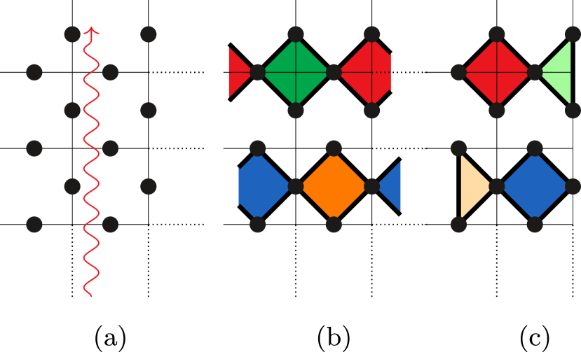
Figure 1: (a) The red snake represents the interpolation cut. (b) TC with periodic boundaries i.e., on a torus. (c) TC with mixed boundaries on a cylinder. The red (blue) diamond represents the $A_{v}^{\mathbin{\blacklozenge}}$ ($B_{p}^{\mathbin{\blacklozenge}}$) interaction whose interaction strength is unperturbed by the interpolation. As a result of interpolation the dark green (orange) full diamonds get mapped to light green (light orange) half diamonds and thereby the interaction is given by $(1-\lambda)A_{v}^{\mathbin{\blacklozenge}}-\lambda A_{v}^{\operatorname*{\text{\raisebox{0.75346pt}{\scalebox{1.0}{$\blacktriangleleft$}}}}}$, $[(1-\lambda)B_{p}^{\mathbin{\blacklozenge}}-\lambda B_{p}^{\operatorname*{\text{\raisebox{0.75346pt}{\scalebox{1.0}{$\blacktriangleright$}}}}}]$.

From Eq. 2, we infer that at $\lambda$ = 0, $H_{pm}(0)$, represents the TC Hamiltonian on torus while at $\lambda=1$, $H_{pm}(1)$, represents the TC Hamiltonian on cylinder with mixed boundary conditions. As the system is perturbed by varying $\lambda$ from 0 to 1, the GSD changes from 4 to 1, indicating the presence of a TPT. The above TPT is accompanied by break in both parity conservation and anyonic symmetry, as in the limit of $\lambda=0$ both are conserved while in the limit of $\lambda=1$ both the symmetries remain broken. We study the energy gap opening in the degenerate manifold, Topological Entanglement Entropy (TEE) with respect to different cuts and the expectation value of open-loop operator to gain further insight into the nature of phase transition.

3.1.1 Energy gap

The ground state of the Hamiltonian, $H_{pm}(\lambda)$, both at $\lambda=0$ and at $\lambda=1$ is given by $\mathcal{N}\prod\limits_{v}(\mathds{1}+A_{v})\ket{\textbf{0}}$, where the product is modified to include the vertices in respective topologies and $\mathcal{N}$ is the normalization constant. In the limit of $\lambda=0$, the action of the non-trivial loop operators around the legs of the torus maps between different degenerate ground states. Since we consider a torus of genus one, the number of non-trivial loop operators are four, thereby the GSD is 4. While in the limit of $\lambda=1$, the non-trivial loop operator, along the periodic boundary of the cylinder, leaves the ground state invariant, thereby we have a unique ground state [24]. Therefore, for some critical strength, $\lambda_{c}$, we expect a gap opening in the degenerate ground state spectrum, as in, Fig. 2.

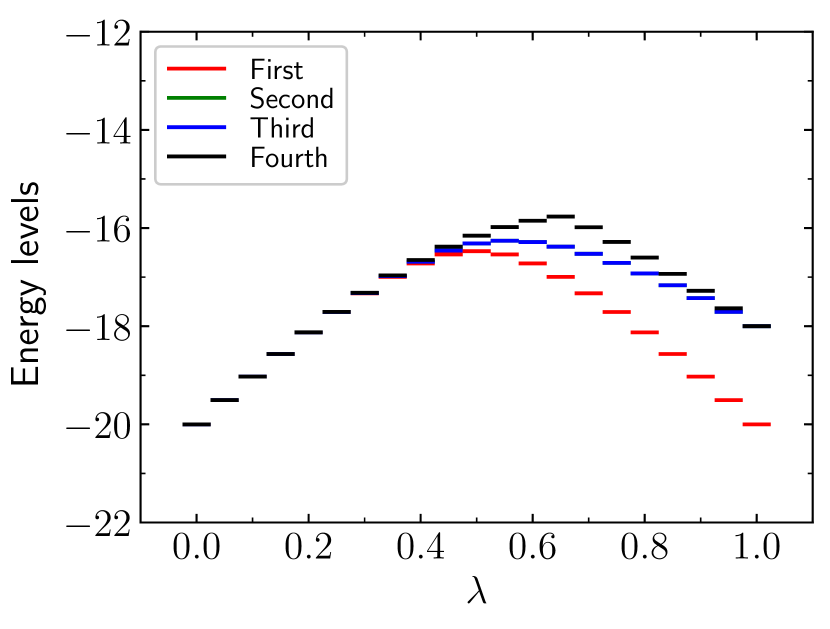
Figure 2: The least energy levels for a system size of $N=20$. At $\lambda=0$, we see that the ground state spectrum is degenerate, while in the limit of $\lambda=1$ we have a unique ground state.

From Fig. 3, we note that there is a suppression in the energy gap $\Delta E$, with increase in the system size, implying the ground state manifold is degenerate upto a critical strength and from its derivative we infer that the critical strength is around 0.5. We note that for the computation of relevant low energy spectrum and relevant ground state properties we have used the linear algebra routines of Julia[25].

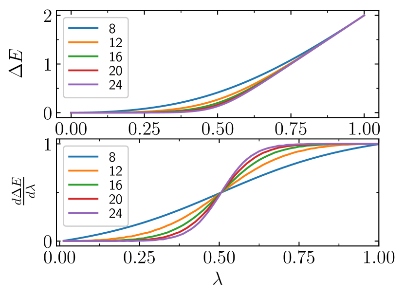
Figure 3: (Top) Difference between the least two energy levels, $\Delta E$ (Bottom) $\frac{d\Delta E}{d\lambda}$, with the labels correponding to different system sizes.

3.1.2 Topological Entanglement Entropy

A key signature of topological order is the constant subleading term in the entanglement entropy, called the Topological Entanglement Entropy (TEE), $\gamma$ [26, 27]. To compute $\gamma$, we refer to the procedure outlined in Ref. [28]. The cut used in the computation of $\gamma$ scales with the radius of the mixed boundary cylinder as in Fig. 4(a).

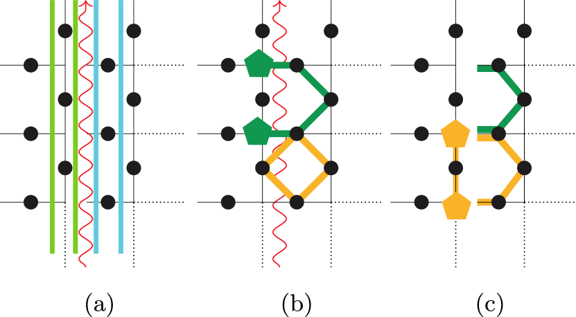
Figure 4: (a) The cuts used in the computation of TEE, the green and blue regions capture a strip on the torus while in the mixed boundary scenario, the green region captures the smooth boundary and the blue region captures the rough boundary. (b) TC on a torus, the green string represents the $\sigma_{z}$ open-loop operator while the golden string represents the trivial Wilson loop operator. (c) Due to the condensation of the excitation at the boundary the green string reduces to a trivial open string while the Wilson loop splits into two open strings, one identical to the green string while the other sporting two excitations at its ends (excitations are denoted by pentagons).

.

From Fig. 5, we note that the TEE is around $\log 2$ for all $\lambda$ and attribute the deviation from $\log 2$ to finite size effects, as reported earlier in Ref. [2]. We further strengthen the claim from the above reference, that TEE is ineffective in detecting a phase transition between two different topological phases.

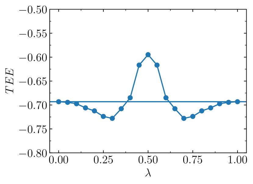
Figure 5: Topological Entanglement Entropy (TEE) as a function of the interpolation strength, $\lambda$.

3.1.3 Open-loop operator

We introduce the open-loop operator as in Fig. 4(b) with periodic boundary as the reference. The open-loop operators are generated by a sequence of $\sigma_{z}^{(i)}(\sigma_{x}^{(j)})$ operators and are marked with excitations at their ends. Let us consider the open-loop operator as in Fig. 4(b), the expectation value with respect to the ground state at $\lambda=0$ is zero, i.e., $\braket{\psi_{gs}^{\lambda=0}}{L_{z}^{r}}{\psi_{gs}^{\lambda=0}}$ = 0, as the loop operator projects the ground state into an excited state. While on the other hand at $\lambda=1$, $\braket{\psi_{gs}^{\lambda=1}}{L_{z}^{r}}{\psi_{gs}^{\lambda=1}}$ = 1, since the excitations at the end of the open-loop condense on the boundary leaving the ground state invariant. We note that the expectation value of the longest open-loop operator i.e., the operator connecting excitations which are maximally separated, effectively captures the phase transition. From Fig. 6 and by performing finite size analysis, we infer that the expectation value diverges at critical strength of $\lambda_{c}=0.533\pm.032$, thereby signalling a phase transition.

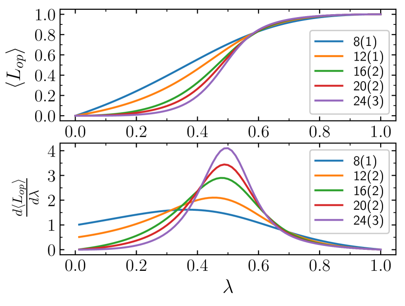
Figure 6: (Top) Expectation value of the longest open-loop operator (Bottom) Derivative of the expectation value with respect to $\lambda$. The labels denote different system sizes with the value in the parentheses indicating the maximal possible separation between the excitations used for the construction of the longest open loop operator.

3.2 Boundary variation: Cylinder with rough boundaries to a mixed boundary

In this section, we consider the TC Hamiltonian on a cylinder and interpolate between rough boundary on both ends to a mixed boundary. The phase transition is similar to topology interpolation case as the GSD varies from 2 to 1 as we vary the interpolation strength. The phase transition is marked by the break in the parity conservation of the $m$-type excitations, as at $\lambda=0$ the $m$-type excitations always appear in pairs while at $\lambda=1$ single excitations can be drawn from the boundary. We also note that there is no anyonic symmetry present in the limits of $\lambda=0$ and $\lambda=1$. We interpolate the right rough boundary to a smooth boundary while the left boundary remains unperturbed, see Fig. 7. To this extent, we decorate the right boundary, $R$, with additional spins denoted by $\blacksquare$ as in Fig. 7 and thereby add additional terms to the Hamiltonian, like $B_{p}^{\boxdot}$, the projector ${\ket{0}\bra{0}}$ as in Eq. 3, which facilitate the interpolation while effectively retaining the boundary properties.

$$\begin{gathered}\begin{split}H_{rm}(\lambda)&=-\sum_{v}A_{v}^{\mathbin{\blacklozenge}}-\sum_{p}B_{p}^{\operatorname*{\text{\raisebox{0.75346pt}{\scalebox{1.0}{$\blacktriangleright$}}}}}\\ &-(1-\lambda)\sum_{p\in R}B_{p}^{\boxdot}-(1-\lambda)\sum_{\blacksquare\in R}\ket{0}\bra{0}\\ &-\lambda\sum_{v\in R}A_{v}^{\operatorname*{\text{\raisebox{0.75346pt}{\scalebox{1.0}{$\blacktriangleleft$}}}}}-\lambda\sum_{p\in R}B_{p}^{\mathbin{\blacklozenge}},\end{split}\end{gathered}$$ (3)

where $A_{v}^{\mathbin{\blacklozenge}}$, $B_{p}^{\mathbin{\blacklozenge}}$, $A_{v}^{\operatorname*{\text{\raisebox{0.75346pt}{\scalebox{1.0}{$\blacktriangleleft$}}}}}$, $B_{p}^{\operatorname*{\text{\raisebox{0.75346pt}{\scalebox{1.0}{$\blacktriangleright$}}}}}$ are as defined in Sec. 3.1. At $\lambda=0$, the above Hamiltonian reduces to the case of rough boundary at both open ends as the right boundary spins are projected to $\ket{0}$ [10], captured by the projector $\ket{0}\bra{0}$ and the typical $B_{p}=\prod\limits_{j}\sigma_{z}^{(j)}$ face interaction at the boundary has to be modified to include the projection at the boundary and therefore modifies itself as $B_{p}^{\boxdot}$, given by

$$B_{p}^{\boxdot}=\frac{1}{2}(\mathds{I}^{\bullet}\mathds{I}^{\bullet}\mathds{I}^{\bullet}+\sigma_{z}^{\bullet}\sigma_{z}^{\bullet}\sigma_{z}^{\bullet})(\frac{\mathds{1}+\sigma_{z}}{2})^{\blacksquare}$$ (4)

where $\bullet$ indicates the action on the spins from the bulk and $\blacksquare$ indicates the action on the spin of the boundary.

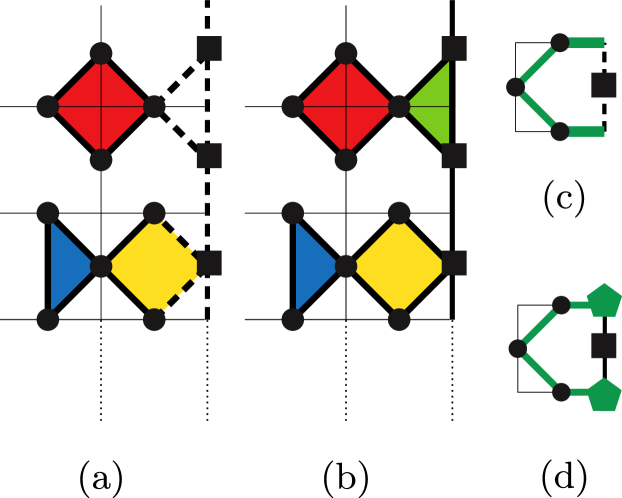
Figure 7: (a) TC on a cylinder with a rough boundary on both ends ($\lambda=0$). Additional spins are added on the right boundary, represented by $\blacksquare$. (b) TC on a cylinder with mixed boundaries. In both (a), (b) the red diamond remains unperturbed with action on the attached edges given by $A_{v}^{\blacklozenge}$, the dark blue half diamond also remains unperturbed with the action on the attached edges given by $B_{p}^{\operatorname*{\text{\raisebox{0.75346pt}{\scalebox{1.0}{$\blacktriangleright$}}}}}$. The yellow diamond in (a) represents the $B_{p}^{\boxdot}$ which translates to $B_{p}^{\blacklozenge}$ in (b), while the uncolored dashed half diamond in (a) maps to $A_{v}^{\operatorname*{\text{\raisebox{0.75346pt}{\scalebox{1.0}{$\blacktriangleleft$}}}}}$ in (b) due to the interpolation. The action of open-loop operator at the boundary at (c) $\lambda=0$, (d) $\lambda=1$.

3.2.1 Energy gap

At $\lambda=0$ and at $\lambda=1$, using the fact that the ground state is a simultaneous ground state of all the operators in the Hamiltonian, one of the ground state can be represented as $\mathcal{N}\prod\limits_{v}(\mathds{1}+A_{v})\ket{\textbf{0}}$, with the product modified suitably to include vertices depending on the value of $\lambda$. In the limit of $\lambda=0$, the ground state manifold is double degenerate [24], while in the limit of $\lambda=1$, the ground state is unique, see Fig. 8. In addition we note that the nature of the energy difference plot, $\Delta E$ versus $\lambda$, is similar to Fig. 3 with the critical strength around 0.5.

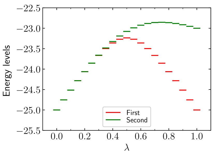
Figure 8: Low energy spectrum of the interpolating Hamiltonian $H_{rm}(\lambda)$ for a system size of $N=20$ spins.

3.2.2 Open-loop operator

As in the topology variation case, we compute the expectation value of the longest open-loop operator. With reference to the rough boundary, the open-loop operator has excitations condensing at the boundary at $\lambda=0$, therefore the expectation value is 1, where as at $\lambda=1$ the excitations are retained at the boundary, see Fig. 7(c), (d), with the expectation value going to zero. From Fig. 9 and by performing finite size analysis we note that the expectation value diverges at $\lambda_{c}=0.481\pm 0.048$.

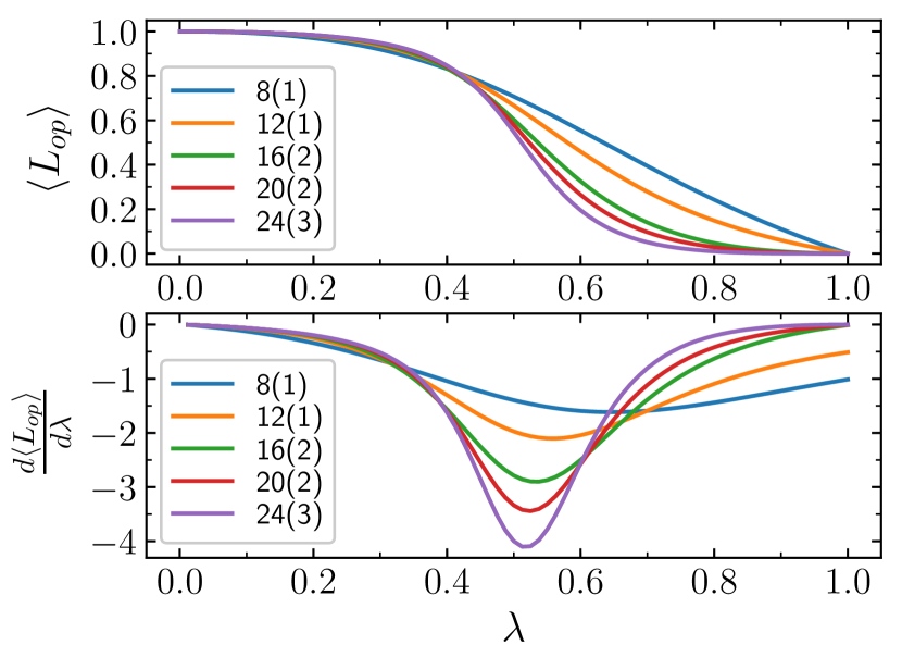
Figure 9: (Top) Expectation value of the longest open-loop operator with respect to the interpolation strength, $\lambda$. (Bottom) Derivative of the expectation value of the open-loop operator with respect to $\lambda$. The labels denote the different system sizes with the value in the parantheses as defined above in Fig. 6.

4 TPT’s: $\tilde{G}_{\lambda=0}=\tilde{G}_{\lambda=1}$

In this section, we introduce various scenarios where the phase transitions are characterized by closing of the energy gap between the ground state manifold and the first excited state along the path of interpolation. We investigate for such cases in the context of topology variation as well as boundary variation.

4.1 Topology variation: Torus with domain wall to a cylinder with rough boundaries

We briefly motivate the notion of domain wall as one of the boundaries of the TC and then further discuss the presence of TPT as we dissect the torus along the domain wall to a cylinder with rough boundaries at either end.

The authors in Ref. [10] have introduced the notion of domain walls between two different TO phases, given by the quantum doubles $D(G_{1})$, $D(G_{2})$. Further, it has been shown that the domain walls between such quantum doubles are equivalent to the boundary conditions of the folded quantum double $D(G_{1}\times G_{2})$, which are characterized by the subgroups, $K$, of $G_{1}\times G_{2}$, along with a non-trivial 2-cocycle of $K$. In the case of folded toric code which is given by $D(Z_{2}\times Z_{2})$, there exists a domain wall given by the subgroup $Z_{2}\times Z_{2}$ along with a non-trivial 2-cocycle of $Z_{2}\times Z_{2}$ which when unfolded reduces to a boundary as illustrated in Fig. 10(b). The Hamiltonian of the TC with a domain wall is given by $H_{dr}(0)$, as in Eq. 5. The modified $B_{p}$ operator at the domain wall, $B_{p}^{\boxplus}$, takes the form as in Fig. 10(d)[11, 29]. The interpolating Hamiltonian connecting the TC with a domain wall on torus to TC on a cylinder with rough boundaries is given by Eq. 5

$$\begin{gathered}\begin{split}H_{dr}(\lambda)&=-\sum_{v}A_{v}^{\mathbin{\blacklozenge}}-\sum_{p}B_{p}^{\mathbin{\blacklozenge}}\\ &-(1-\lambda)\sum_{p^{\prime}}B_{p}^{\boxplus}\\ &-\lambda\sum_{p^{\prime\prime}}B_{p}^{\operatorname*{\text{\raisebox{0.75346pt}{\scalebox{1.0}{$\blacktriangleleft$}}}}}-\lambda\sum_{p^{\prime\prime}}B_{p}^{\operatorname*{\text{\raisebox{0.75346pt}{\scalebox{1.0}{$\blacktriangleright$}}}}},\end{split}\end{gathered}$$ (5)

where $A_{v}^{\mathbin{\blacklozenge}}$, $B_{p}^{\mathbin{\blacklozenge}}$, $B_{p}^{\operatorname*{\text{\raisebox{0.75346pt}{\scalebox{1.0}{$\blacktriangleright$}}}}}$ are defined as in Sec. 3.1, while $B_{p}^{\operatorname*{\text{\raisebox{0.75346pt}{\scalebox{1.0}{$\blacktriangleleft$}}}}}$ is qualitatively identical to $B_{p}^{\operatorname*{\text{\raisebox{0.75346pt}{\scalebox{1.0}{$\blacktriangleright$}}}}}$. The phase transition is characterized by break in the parity and anyonic symmetry. The parity of the $m$-type excitations is preserved in the limit of $\lambda=1$ while is broken in the limit of $\lambda=0$. On the other hand, anyonic symmetry is preserved in the limit of $\lambda=0$ and is broken in the limit $\lambda=1$.

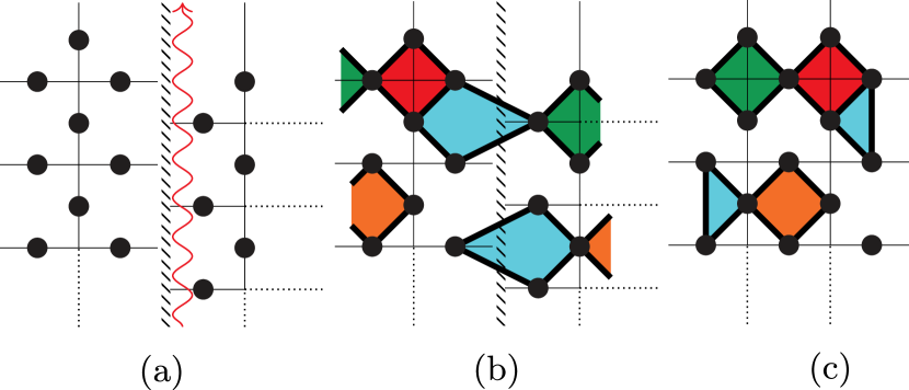
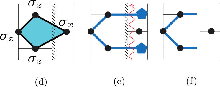
Figure 10: (a) The interpolation cut, denoted by the red snake dissects along the domain wall. (b) At $\lambda=0$, TC on a torus with a domain wall, denoted by the short slant interface. (c) At $\lambda=1$, TC on a cylinder with a rough boundary on both ends. (d) $B_{p}^{\boxplus}$ operator at the domain wall. (e) Open-loop operator with a pair of excitations projecting the ground state at $\lambda=0$ into an excited state. (f) Open-loop operator whose excitations have condensed at the boundary leaving the ground state at $\lambda=1$ invariant under the loop action.

4.1.1 Energy gap

At both $\lambda=0$ and $\lambda=1$, the ground state manifold is two fold degenerate. Using the notion established in the earlier sections, one of the representations of the ground state at $\lambda=0$ is given by $\mathcal{N}\prod_{v}(\mathds{1}+A_{v})\prod_{p}(\mathds{1}+B_{p}^{\boxplus})\ket{\textbf{0}}$, where as at $\lambda=1$, is given by $\mathcal{N}\prod_{v}(\mathds{1}+A_{v})\ket{\textbf{0}}$. In the limit of $\lambda=0$, the other ground state can be obtained by the action of the non-trivial loop operator running parallel to the domain wall. The other non-trivial loop operator running perpendicular to the domain wall does not leave the ground state invariant as $m$-type violations get identified as $e$-type violations as they pass through the domain wall, the fusion of which results in a fermion, instead of vacuum, as in the absence of the domain wall. Therefore, establishing the fact that the GSD of the TC with a domain wall on torus is two. From Fig. 11, for finite size system of $N=20$ spins, we see a split in the ground state manifold around $\lambda=0.5$ and also note that the first and the second excited states merge.

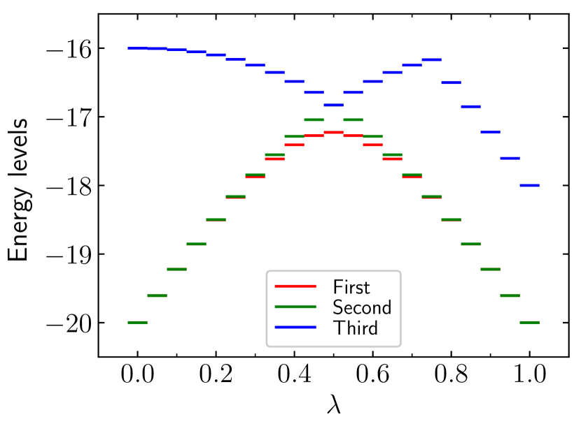
Figure 11: The least energy levels for a system size of $N=20$. At $\lambda=0$ and $\lambda=1$, we note that the ground state manifold is degenerate, while around $\lambda=0.5$, we note the split in the degeneracy along with the the merging of the first and second excited states.

From Fig. 12, we note that the energy gap between the ground state and the first excited state decreases with increase in system size. Extrapolating to the thermodynamic limit by performing finite size analysis, we note that the degeneracy of the ground state manifold is retained at all $\lambda$ and combining the fact that there is a energy gap closing at $\lambda=0.5$ results in a energy spectrum as in Fig. 13 indicating the presence of a TPT at $\lambda=0.5$.

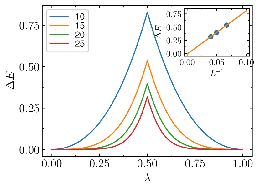
Figure 12: Energy difference between the first two energy levels as a function of the interpolation strength, $\lambda$, with the labels denoting the different system sizes (Inset) Extrapolating the energy difference at $\lambda=0.5$, to the thermodynamic limit by performing finite-size analysis.

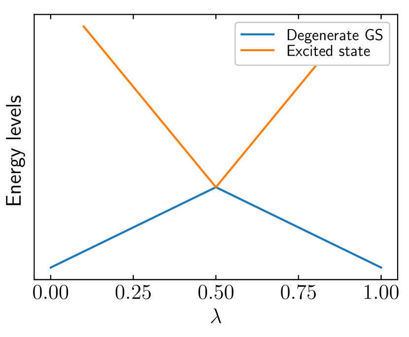
Figure 13: The potential energy spectrum in the thermodynamic limit as a function of the interpolation strength, $\lambda$. The gap closing between the degenerate ground state manifold and the first excited state indicates the presence of the phase transition.

4.1.2 Open-loop operator

To further consolidate the presence of TPT, we compute the expectation value of the longest open-loop operator at different interpolation strength, $\lambda$. We define the loop operator with reference to the TC on a torus with a domain wall as in Fig. 10(e). The open-loop is generated by the action of a sequence of $\sigma_{z}$ operators and sports two $B_{p}$ violations at its end. In this limit of $\lambda=0$, the loop operator projects the ground state into an excited state, thereby leading to an expectation value of zero. While at the other extreme, $\lambda=1$, the excitations at the end of the open-loop condense at the boundary, as in Fig. 10(f), thereby leaving the ground state invariant and hence the expectation value is one in the vicinity of $\lambda=1$. From Fig. 14 and by performing finite size scaling analysis we conclude that the critical strength is given by $\lambda_{c}=0.539\pm 0.046$,

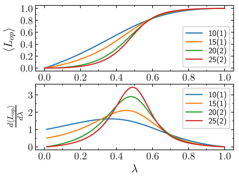
Figure 14: (Top) Expectation value of the longest open-loop operator with respect to different interpolation strength, $\lambda$. (Bottom) Derivative of the expectation value with respect to $\lambda$. The labels denote the different system sizes with the value in the parantheses as defined earlier.

4.2 Boundary variation: Cylinder with rough boundaries to smooth boundaries

In this section we present the boundary variation of the above TPT. To this extent, we interpolate between rough boundary on both ends to smooth boundary on both ends of the cylinder, see Fig. 15(a), (b). The interpolating Hamiltonian is given by $H_{rs}$, as in Eq. 6.

$$\begin{gathered}\begin{split}H_{rs}(\lambda)&=-\sum_{v\in I}A_{v}^{\mathbin{\blacklozenge}}\\ &-(1-\lambda)\sum_{p\in R}B_{p}^{\boxdot}-(1-\lambda)\sum_{p\in L}B_{p}^{\boxdot}\\ &-(1-\lambda)\sum_{\blacksquare\in R}\ket{0}\bra{0}-(1-\lambda)\sum_{\blacksquare\in L}\ket{0}\bra{0}\\ &-\lambda\sum_{v\in R}A_{v}^{\operatorname*{\text{\raisebox{0.75346pt}{\scalebox{1.0}{$\blacktriangleleft$}}}}}-\lambda\sum_{v\in L}A_{v}^{\operatorname*{\text{\raisebox{0.75346pt}{\scalebox{1.0}{$\blacktriangleright$}}}}}\\ &-\lambda\sum_{p\in R}B_{p}^{\mathbin{\blacklozenge}}-\lambda\sum_{p\in L}B_{p}^{\mathbin{\blacklozenge}},\end{split}\end{gathered}$$ (6)

where $I$ denotes the interior bulk region, $R$ denotes the right boundary and $L$ denotes the left boundary. The phase transition is characterized by break in the parity conservation of the $m(e)$-type excitations. In the limit of $\lambda=0$, $m(e)$-type excitations occur in pairs (singly) while in the limit of $\lambda=1$, $m(e)$-type excitations appear singly (in pairs). There is no anyonic symmetry present in either phases due to the condensation at the boundary i.e., the fusion rules are not invariant under the exchange of $e$ and $m$ labels.

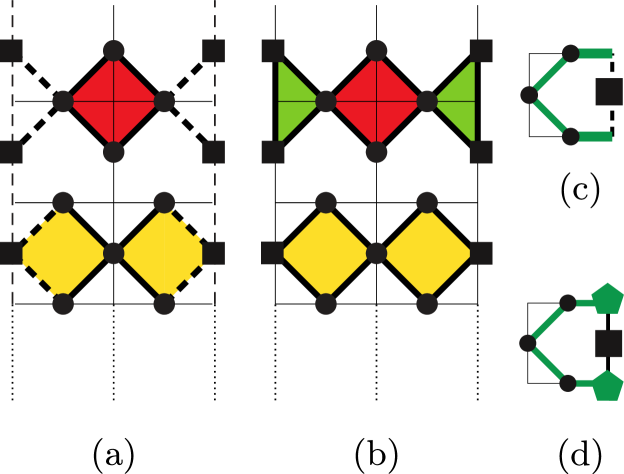
Figure 15: TC on a cylinder with (a) rough boundary, (b) smooth boundary on both ends. The red diamond belongs to the interior region, $I$, which remains unperturbed while the transparent half diamonds in (a) translate to half filled green diamonds $A_{v}^{\operatorname*{\text{\raisebox{0.75346pt}{\scalebox{1.0}{$\blacktriangleleft$}}}}}$, $A_{v}^{\operatorname*{\text{\raisebox{0.75346pt}{\scalebox{1.0}{$\blacktriangleright$}}}}}$ at either boundaries $L$ and $R$ respectively as $\lambda$ varies from 0 to 1. Similarly, the golden yellow diamonds represent $B_{p}^{\boxdot}$ in (a) and map to $B_{p}^{\mathbin{\blacklozenge}}$ in (b) with increase in $\lambda$. The action of the open-loop operator at the boundary at (c) $\lambda=0$, (d) $\lambda=1$.

4.2.1 Energy gap

The ground state manifold is two fold degenerate at the extremities of the interpolation parameter, $\lambda$ [24]. As in the case of topology variation, it is evident that for finite size systems the first and the second excited states merge at $\lambda=0.5$, see Fig. 16. The energy difference between the first two energy levels is qualitatively similar to Fig. 12 and thereby in the thermodynamic limit the energy spectrum qualitatively resembles Fig. 13, implying the presence of a phase transition due to the closure of the energy gap.

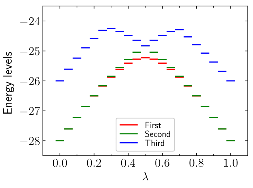
Figure 16: Least energy levels for a system size of $N=20$ spins. Both at $\lambda=0$ and $\lambda=1$, the ground state manifold is degenerate. At $\lambda=0.5$, we note the merging of the first and the second excited energy levels.

4.2.2 Open-loop operator

Taking cue from the above analysis, we compute the expectation value of the open-loop operator to estimate the critical strength at which the phase transition occurs. The open-loop operator is generated by a sequence of $\sigma_{z}$ operators which holds $A_{v}$ excitations at its end. At $\lambda=0$, these excitations condense on the boundary, while at $\lambda=1$, the excitations are retained at the boundary as in Fig. 15(c), (d) respectively. From Fig. 17, and by performing finite size analysis we note that the expectation value diverges at $\lambda_{c}=0.463\pm 0.036$.

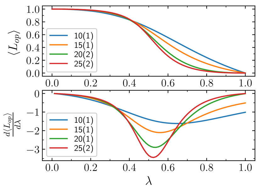
Figure 17: (Top) Expectation value of the longest open-loop operator with respect to $\lambda$. (Bottom) Derivative of the expectation value with respect to $\lambda$. As noted earlier, the labels denote the different system sizes.

5 Interpolation via engineered dissipation

We aim to achieve the interpolation introduced in Sec. 3.1, in an open quantum system by engineering suitable collapse operators. To draw parallels with the closed system analysis, the study of phase transitions in open systems is associated with the properties of the steady states which are obtained by solving the Lindblad Master equation (LME)

$$\begin{gathered}\dot{\rho}(t)=-i[H(t),\rho(t)]+\\ \sum\limits_{n}\frac{1}{2}[2C_{n}\rho(t)C_{n}^{\dagger}-\rho(t)C_{n}^{\dagger}C_{n}-C_{n}^{\dagger}C_{n}\rho(t)]\end{gathered}$$ (7)

where $H$ is the Hamiltonian capturing coherent evolution while $C_{n}$’s are the collapse operators which encode the dissipative dynamics.

In Ref. [20], the authors have introduced collapse operators which cool a product state to the entangled ground state of the TC. We consider a purely dissipative setup i.e., set $H$=0 and extend the above construction, by introducing additional collapse operators whose effective cooling rate involves the interpolation parameter, $\lambda$, thereby cooling to different ground states at the extremities of the interpolation. We analyze the case of interpolation between the ground state of TC on a torus ($\lambda=0$) to the ground state on a cylinder with mixed boundary conditions ($\lambda=1$) as introduced in Sec. 3.1. For lucidity, we split the collapse operators into three classes: the collapse operators acting on the permanent vertices (faces) given by $c_{v(f)}^{p}$, the collapse operators acting on the periodic boundary given by $c_{v(f)}^{t}$ and the collapse operators acting on the open boundary given by $c_{v(f)}^{o}$ and define them as in Eq. 8, Fig. 18.

$$\begin{gathered}\begin{split}c_{v}^{p}&=\frac{\sqrt{\gamma_{v}}}{2}\sigma_{z}^{(i)}(\mathds{1}-A_{v}^{\mathbin{\blacklozenge}}),\\ c_{f}^{p}&=\frac{\sqrt{\gamma_{f}}}{2}\sigma_{x}^{(j)}(\mathds{1}-B_{f}^{\mathbin{\blacklozenge}}),\\ c_{v}^{t}(\lambda)&=\frac{\sqrt{\gamma_{v}}}{2}(1-\lambda)\sigma_{z}^{(i)}(\mathds{1}-A_{v}^{\mathbin{\blacklozenge}}),\\ c_{f}^{t}(\lambda)&=\frac{\sqrt{\gamma_{f}}}{2}(1-\lambda)\sigma_{x}^{(j)}(\mathds{1}-B_{f}^{\mathbin{\blacklozenge}}),\\ c_{v}^{o}(\lambda)&=\frac{\sqrt{\gamma_{v}}}{2}\lambda\sigma_{z}^{(i)}(\mathds{1}-A_{v}^{\operatorname*{\text{\raisebox{0.75346pt}{\scalebox{1.0}{$\blacktriangleright$}}}}}),\\ c_{f}^{o}(\lambda)&=\frac{\sqrt{\gamma_{f}}}{2}\lambda\sigma_{x}^{(j)}(\mathds{1}-B_{f}^{\operatorname*{\text{\raisebox{0.75346pt}{\scalebox{1.0}{$\blacktriangleleft$}}}}}),\end{split}\end{gathered}$$ (8)

where $\gamma_{v},\gamma_{f}$ are the cooling rates of the vertex and face excitations, while $\lambda$ is the interpolation strength, $A_{v}^{\mathbin{\blacklozenge}}$, $B_{f}^{\mathbin{\blacklozenge}}$, $A_{v}^{\operatorname*{\text{\raisebox{0.75346pt}{\scalebox{1.0}{$\blacktriangleright$}}}}}$, $B_{f}^{\operatorname*{\text{\raisebox{0.75346pt}{\scalebox{1.0}{$\blacktriangleleft$}}}}}$ operators are as defined in the earlier sections. Intuitively, the dynamics induced by the collapse operators diffuse the excitations around the lattice i.e., the excitations perform a random walk and upon meeting another excitation or a relevant boundary, fuse, thereby cooling to a steady state. In the limit of $\lambda=0$ and $\lambda=1$, the collapse operators effectively cool the product state to a pure steady state given by ground state of the TC at respective $\lambda$. At intermediate $\lambda$, the dynamics is captured by the competition between the cooling operators that promote the diffusion of the excitations along the periodic boundary and the cooling operators which promote a biased diffusion resulting in a restricted diffusion, effectively capturing the break in topology. Due to the competitive cooling, the steady state at intermediate $\lambda$ is a mixed state unlike the pure steady state at the extremities, hence the phase transition which we shall present shortly is a mixed state phase transition. We further note that the phase transition analysis presented hereafter, is based on the assumption that the steady state at all $\lambda$ is TO, thereby resulting in a TPT in an open system. The assumption can be substantiated by the fact that the mixed state obtained at intermediate $\lambda$, in the end, is due to a collective cooling scheme where the cooling itself is aimed at generating a TO pure state. We aim to present other signatures for detecting QPT’s between TO and trivial mixed states in a separate work and hence the verification shall be postponed to the future[30].

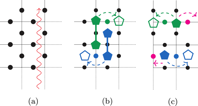
Figure 18: (a) The red snake represents the interpolation cut. The dissipative dynamics induced by the collapse operators by diffusing excitations on (b) a torus (c) a cylinder with mixed boundaries. (b) Excitations always appear in pairs and the collapse operators diffuse the excitations (represented by dashed green and blue arrows) or cool them by fusing (represented by thick green and blue lines). (c) Excitation parity is not conserved because of the boundary, thereby allowing the excitations to condense at the boundary (represented by dashed magenta arrows), in addition to the diffusion and pair cooling as noted in (b).

We compute the steady states at different interpolating strength, $\lambda$, by using the Monte Carlo Wave Function (MCWF) method [31]. In the vicinity of $\lambda=0$, the dissipators cool the system to the ground state of the TC on a torus while at $\lambda=1$, the dissipators cool the system to the ground state of the TC on a cylinder. The expectation value of the open-loop operator, given by $\operatorname{Tr}({\rho_{\lambda}L})$ where $\rho_{\lambda}$ is the steady state at interpolation strength $\lambda$ and $L$ is the open-loop operator, as in Fig. 4(b), is used to distinguish the different topological phases. Using similar arguments presented earlier, we note that the expectation value of the open-loop operator is zero in the periodic boundary case where as is 1 in the open boundary case, with the critical strength at $\lambda_{c}=0.637\pm.004$ obtained by performing finite size analysis, as in Fig. 19.

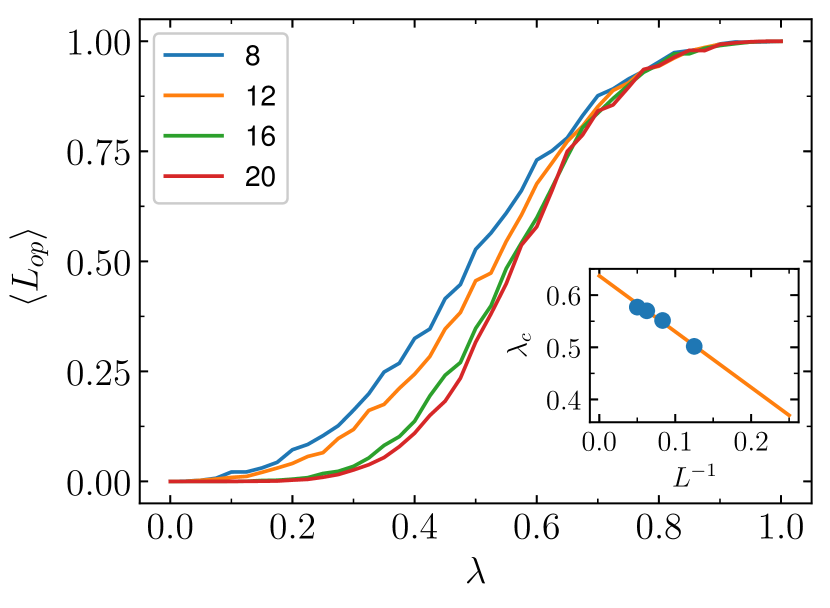
Figure 19: Expectation value of the longest open-loop operator with respect to the interpolation strength, $\lambda$ with the labels denoting the different system sizes. (Inset) Finite size scaling to obtain the critical strength, $\lambda_{c}$.

6 Summary and Discussion

In summary, we have studied the sensitivity of topological phases with respect to the boundary conditions of the underlying manifold on which they are defined. We have considered the change in boundary conditions of two flavors: (a) effective topology variation, where we have varied the underlying topology from periodic boundary to open boundary i.e., from torus to a cylinder (b) effective boundary variation, where we have fixed the underlying topology to a cylinder and have varied the open boundaries of the cylinder. The sensitivity to the boundary conditions is captured by a phase transition, termed as TPT, as we interpolate by Hamiltonian deformation between different boundary conditions. We have invoked the notion of parity conservation and anyonic symmetries and have established that a break in either one of the above symmetries is sufficient to characterize the TPT. To further consolidate the presence of a TPT, we have numerically analyzed signatures such as ground state degeneracy, TEE and have introduced the notion of open-loop operator whose expectation value captures the phase transition. While the ground state degeneracy and expectation value of the open-loop operator provide an estimate of the critical strength, we have re-established the fact that TEE remains constant and is thereby ineffective in detecting the above introduced TPT’s.

Having established the notion of TPT in a closed setup, we extend it to an open quantum setup. The phase transitions in an open setting are associated with the steady states obtained by solving the LME. To this extent, we have introduced collapse operators, whose dissipative rates are a function of the interpolation parameter $\lambda$. Due to the above construction, the dynamics cool the product state into distinct TO steady states at different $\lambda$, with the extremities being mapped to the relevant TC ground states, thereby encoding a TPT at some critical $\lambda$. We have shown that the expectation value of the open-loop operator is still relevant and is effective in detecting such TPT’s in an open setup.

In this paper, having analyzed the presence of TPT’s in various closed and open setups, it would be interesting to gain an insight into the stability of topological order due to different boundaries, in a dynamical setting as the system is quenched across a TPT [32]. The introduced TPT’s being characterized by non-local order parameter, it would be interesting to study the notion of Kibble-Zurek like mechanism in both closed and open setting [33]. There has been a recent proposal to define topological phases in the context of open quantum systems [34], it would be interesting to study the TPT in an open setup introduced in this work with the above definition. Experimentally, there has been progress in realizing the ground states of the TC Hamiltonian as in Ref. [14], which also includes open system scenarios with various noise protocols, it would be interesting to study the realization of proposed engineered collapse operators in such a setup. Also, there has been recent progress in preparing quantum states using variational quantum circuits [35], it would be interesting to extend the above protocol to realize the interpolated topological steady states by including suitable variational dissipators. Some of the immediate extensions would be to detect the presence of similar TPT’s in the context of other abelian and non-abelian models with an aim to develop other relevant signatures.

Appendix A Interpolating between mixed boundaries on either end

We interpolate between TC on a cylinder with mixed boundary conditions as in Fig. 20 (we interpolate between (a) and (b) as $\lambda$ is varied from 0 to 1). The TPT is characterized by the energy gap closing at $\lambda=0.5$ and belongs to the class of $\tilde{G}_{\lambda=0}=\tilde{G}_{\lambda=1}$. There is neither parity conservation, as excitations can be singly drawn from the boundary, nor anyonic symmetry, due to the condensation properties at the boundary, for all $\lambda$, implying that it is not necessary that every TPT is accompanied by a broken symmetry. In the main discussion, we referred to the parity being broken with respect to $e,m$-type excitations without laying much emphasis on the choice of the boundary of the cylinder i.e., left or right physical boundary. We observe that by specifying the parity symmetry with respect to a particular physical boundary, allows us to state the following: Either a break in the parity with respect to a particular physical boundary or break in the anyonic symmetry is necessary and sufficient to characterize the presence of a TPT.

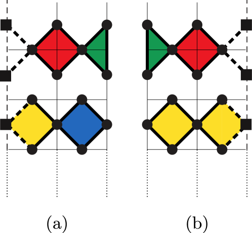
Figure 20: TC on a cylinder with mixed boundary conditions (a) rough boundary on the left and smooth boundary on the right (b) smooth boundary on the left and rough boundary on the right.

Extending the above implication to the current scenario, it is evident that that the parity of $e(m)$-type excitations is preserved with respect to the right (left) physical boundary in the limit of $\lambda=0$, while is broken in the limit of $\lambda=1$. Therefore, we have substantiated that imposing stronger conditions on the parity preservation leads to a bi-implication between the presence of TPT and the parity conservation, anyonic symmetries. The above statement may be generalized for any abelian quantum doubles, as the parity of atleast one of the superselection sectors is broken due to the condensation at the boundary.

Appendix B TPT’s with the domain wall intact

In every scenario discussed above, we have observed that the TPT is characterized by break in parity conservation of either $e,m$ excitations or both due to the introduction of relevant boundary conditions. In this section, we present a scenario where the TPT is solely characterized by the break in anyonic symmetry with no conservation in parity, at all $\lambda$. To this extent, we consider the TC on a torus with domain wall ($\lambda=0$) and instead of interpolating along the domain wall we cut through the periodic boundary as in Fig. 21 to a cylinder with mixed boundary with the domain wall intact ($\lambda=1)$. The interpolation encodes a TPT as the GSD in the limit of $\lambda=0$ is 2 while in the limit of $\lambda=1$ is 4.

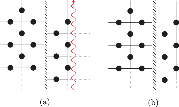
Figure 21: (a) TC on a torus with a domain wall. The red snake represents the interpolation cut which breaks the periodicity along some other rail other than the domain wall leading to (b) TC on a cylinder with mixed boundaries on either end with the domain wall intact.

In the limit of $\lambda=0$, there is no conservation in parity due to the presence of domain wall although the anyonic symmetry is conserved. On the other hand at $\lambda=1$ it is still possible to draw single excitations from the boundary thereby there is no conservation in parity while the anyonic symmetry is also broken due to the introduction of open boundaries. Therefore, in this case the TPT is solely characterized by the break in anyonic symmetry.

Appendix C TPT’s arising out of simultaneous dissection and gluing

In this section, we introduce a TPT arising out of simultaneous dissection and gluing along two different boundaries. To this end, we consider the TC Hamiltonian on cylinder with mixed boundaries along with a domain wall in the limit of $\lambda=0$, being mapped to TC Hamiltonian on a cylinder with a rough boundary at either end in the limit of $\lambda=1$, see Fig. 22.

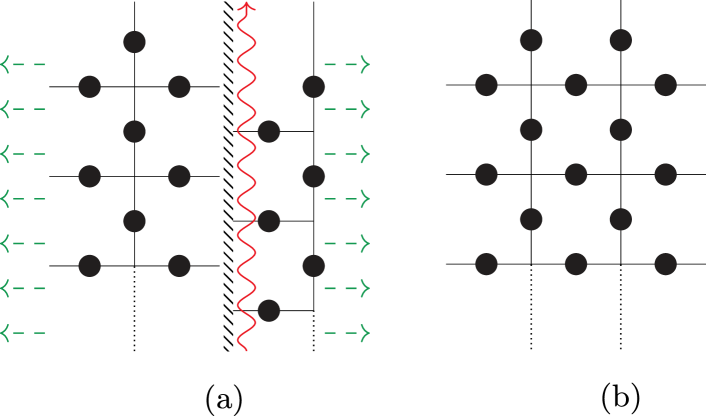
Figure 22: Interpolating via simultaneous dissection and gluing, the red snake represents the dissection while the dashed green arrows represent the gluing action. (a) TC on a clylinder with mixed boundaries and a domain wall (b) TC on cylinder with rough boundaries on either end.

The TPT is marked by the change in GSD as it maps from 4 in the limit of $\lambda=0$ to 2 in the limit of $\lambda=1$. Additionally, we also note that the parity conservation is preserved with respect to $m$-type excitations in the limit of $\lambda=1$ while it remains broken in the limit of $\lambda=0$.

Appendix D Dissipative interpolation via imperfect cooling

In Sec. 5, we have introduced collapse operators whose action leaves the state invariant in the absence of the excitations or diffuse/annihilate the excitations when present. In this section, we introduce collapse operators as in Eq. 9, where the $A_{v}(B_{p})$ operators along the interpolation cut are additionally scaled by the relevant interpolation parameter.

$$\begin{gathered}\begin{split}c_{v}^{t}(\lambda)&=\frac{\sqrt{\gamma_{v}}}{2}(1-\lambda)\sigma_{z}^{(i)}(\mathds{1}-(1-\lambda)A_{v}^{\mathbin{\blacklozenge}}),\\ c_{f}^{t}(\lambda)&=\frac{\sqrt{\gamma_{f}}}{2}(1-\lambda)\sigma_{x}^{(j)}(\mathds{1}-(1-\lambda)B_{f}^{\mathbin{\blacklozenge}}),\\ c_{v}^{o}(\lambda)&=\frac{\sqrt{\gamma_{v}}}{2}\lambda\sigma_{z}^{(i)}(\mathds{1}-\lambda A_{v}^{\operatorname*{\text{\raisebox{0.75346pt}{\scalebox{1.0}{$\blacktriangleright$}}}}}),\\ c_{f}^{o}(\lambda)&=\frac{\sqrt{\gamma_{f}}}{2}\lambda\sigma_{x}^{(j)}(\mathds{1}-\lambda B_{f}^{\operatorname*{\text{\raisebox{0.75346pt}{\scalebox{1.0}{$\blacktriangleleft$}}}}}),\end{split}\end{gathered}$$ (9)

The key difference between these collapse operators and the ones introduced earlier, as in Eq. 8, is given by the fact that in the absence of excitations, the former induces additional excitations while the latter leaves the state invariant. To gain further insight into the phase transition, we compute the expectation value of the open-loop operator with respect to the interpolation strength, $\lambda$, see Fig. 23. By performing finite size analysis, we obtain $\lambda_{c}=0.586\pm 0.001$ which is lower compared to the earlier case.

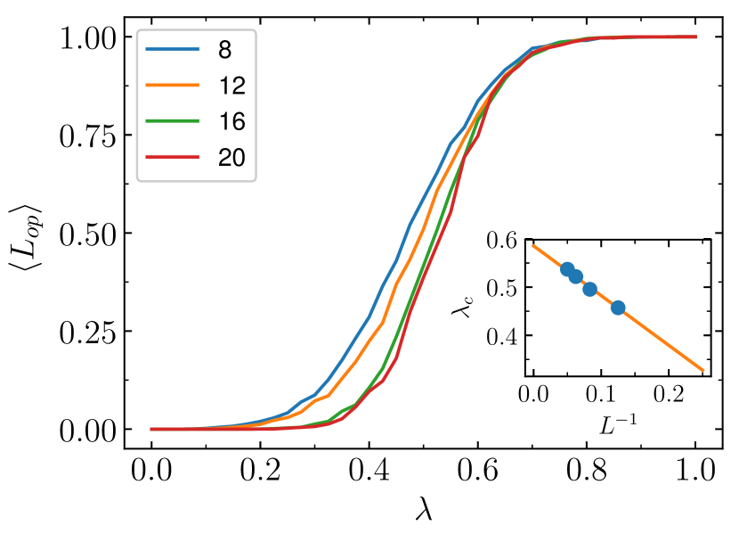
Figure 23: Expectation value of the longest open-loop operator with respect to the interpolation strength, $\lambda$ with the labels denoting the different system sizes. (Inset) Finite size scaling to obtain the critical strength, $\lambda_{c}$.

References

- [1] H.-C. Jiang, Z. Wang, and L. Balents, Identifying topological order by entanglement entropy, Nature Physics 8, 902–905 (2012).
- [2] S. C. Morampudi, C. von Keyserlingk, and F. Pollmann, Numerical study of a transition between topologically ordered phases, Physical Review B 90 (2014).
- [3] M. H. Zarei, Quantum phase transition from to topological order, Phys. Rev. A 93, 042306 (2016).
- [4] Y. Hu, Y. Wan, and Y.-S. Wu, From effective Hamiltonian to anomaly inflow in topological orders with boundaries, Journal of High Energy Physics 2018 (2018).
- [5] M. Iqbal, K. Duivenvoorden, and N. Schuch, Study of anyon condensation and topological phase transitions from a topological phase using the projected entangled pair states approach, Physical Review B 97 (2018).
- [6] C. Castelnovo, S. Trebst, and M. Troyer, Topological Order and Quantum Criticality, Understanding Quantum Phase Transitions , 169–192 (2010).
- [7] B. Yoshida, Classification of quantum phases and topology of logical operators in an exactly solved model of quantum codes, Annals of Physics 326, 15 (2011).
- [8] A. Kitaev, Fault-tolerant quantum computation by anyons, Annals of Physics 303, 2–30 (2003).
- [9] M. A. Levin and X.-G. Wen, String-net condensation: A physical mechanism for topological phases, Phys. Rev. B 71, 045110 (2005).
- [10] S. Beigi, P. W. Shor, and D. Whalen, The Quantum Double Model with Boundary: Condensations and Symmetries, Communications in Mathematical Physics 306, 663–694 (2011).
- [11] A. Kitaev and L. Kong, Models for Gapped Boundaries and Domain Walls, Communications in Mathematical Physics 313, 351–373 (2012).
- [12] I. Cong, M. Cheng, and Z. Wang, Hamiltonian and Algebraic Theories of Gapped Boundaries in Topological Phases of Matter, Communications in Mathematical Physics 355, 645–689 (2017).
- [13] A. G. Fowler, M. Mariantoni, J. M. Martinis, and A. N. Cleland, Surface codes: Towards practical large-scale quantum computation, Physical Review A 86 (2012).
- [14] M. Sameti, A. Potočnik, D. E. Browne, A. Wallraff, and M. J. Hartmann, Superconducting quantum simulator for topological order and the toric code, Phys. Rev. A 95, 042330 (2017).
- [15] H. Weimer, Variational Principle for Steady States of Dissipative Quantum Many-Body Systems, Phys. Rev. Lett. 114, 040402 (2015).
- [16] V. R. Overbeck, M. F. Maghrebi, A. V. Gorshkov, and H. Weimer, Multicritical behavior in dissipative Ising models, Phys. Rev. A 95, 042133 (2017).
- [17] M. Raghunandan, J. Wrachtrup, and H. Weimer, High-Density Quantum Sensing with Dissipative First Order Transitions, Phys. Rev. Lett. 120, 150501 (2018).
- [18] S. Helmrich, A. Arias, and S. Whitlock, Uncovering the nonequilibrium phase structure of an open quantum spin system, Physical Review A 98 (2018).
- [19] F. Carollo, E. Gillman, H. Weimer, and I. Lesanovsky, Critical Behavior of the Quantum Contact Process in One Dimension, Physical Review Letters 123 (2019).
- [20] H. Weimer, M. Müller, I. Lesanovsky, P. Zoller, and H. P. Büchler, A Rydberg quantum simulator, Nature Physics 6, 382–388 (2010).
- [21] X. Chen, Z.-C. Gu, and X.-G. Wen, Local unitary transformation, long-range quantum entanglement, wave function renormalization, and topological order, Physical Review B 82 (2010).
- [22] H. Bombin, Topological Order with a Twist: Ising Anyons from an Abelian Model, Phys. Rev. Lett. 105, 030403 (2010).
- [23] J. C. Y. Teo, Globally symmetric topological phase: from anyonic symmetry to twist defect., Journal of physics. Condensed matter : an Institute of Physics journal 28 14, 143001 (2016).
- [24] J. C. Wang and X.-G. Wen, Boundary degeneracy of topological order, Physical Review B 91 (2015).
- [25] J. Bezanson, A. Edelman, S. Karpinski, and V. B. Shah, Julia: A fresh approach to numerical computing, SIAM review 59, 65 (2017), We have used Base.LinAlg.eigs function to compute the low energy spectrum and the ground state wavefunction.
- [26] A. Kitaev and J. Preskill, Topological Entanglement Entropy, Physical Review Letters 96 (2006).
- [27] M. Levin and X.-G. Wen, Detecting Topological Order in a Ground State Wave Function, Physical Review Letters 96 (2006).
- [28] A. Jamadagni, H. Weimer, and A. Bhattacharyya, Robustness of topological order in the toric code with open boundaries, Physical Review B 98 (2018).
- [29] B. Yoshida, Gapped boundaries, group cohomology and fault-tolerant logical gates, Annals of Physics 377, 387–413 (2017).
- [30] A. Jamadagni and H. Weimer, An Operational Definition of Topological Order, arXiv:2005.06501 (2020).
- [31] J. Johansson, P. Nation, and F. Nori, QuTiP 2: A Python framework for the dynamics of open quantum systems, Computer Physics Communications 184, 1234–1240 (2013), We have used qutip.mcsolve to compute the steady state at a given interpolation strength.
- [32] D. I. Tsomokos, A. Hamma, W. Zhang, S. Haas, and R. Fazio, Topological order following a quantum quench, Physical Review A 80 (2009).
- [33] A. Chandran, F. J. Burnell, V. Khemani, and S. L. Sondhi, Kibble–Zurek scaling and string-net coarsening in topologically ordered systems, Journal of Physics: Condensed Matter 25, 404214 (2013).
- [34] A. Coser and D. Pérez-García, Classification of phases for mixed states via fast dissipative evolution, Quantum 3, 174 (2019).
- [35] C. Kokail, C. Maier, R. van Bijnen, T. Brydges, M. K. Joshi, P. Jurcevic, C. A. Muschik, P. Silvi, R. Blatt, C. F. Roos, and et al., Self-verifying variational quantum simulation of lattice models, Nature 569, 355–360 (2019).
- [36] T. Lichtman, R. Thorngren, N. H. Lindner, A. Stern, and E. Berg, Bulk Anyons as Edge Symmetries: Boundary Phase Diagrams of Topologically Ordered States, arXiv:2003.04328 (2020).