From Artificial Neural Networks to Deep Learning
for Music Generation – History, Concepts and Trends

Abstract: The current wave of deep learning (the hyper-vitamined return of artificial neural networks) applies not only to traditional statistical machine learning tasks: prediction and classification (e.g., for weather prediction and pattern recognition), but has already conquered other areas, such as translation. A growing area of application is the generation of creative content, notably the case of music, the topic of this paper. The motivation is in using the capacity of modern deep learning techniques to automatically learn musical styles from arbitrary musical corpora and then to generate musical samples from the estimated distribution, with some degree of control over the generation. This paper provides a tutorial on music generation based on deep learning techniques. After a short introduction to the topic illustrated by a recent exemple, the paper analyzes some early works from the late 1980s using artificial neural networks for music generation and how their pioneering contributions have prefigured current techniques. Then, we introduce some conceptual framework to analyze the various concepts and dimensions involved. Various examples of recent systems are introduced and analyzed to illustrate the variety of concerns and of techniques.

1 Introduction

Since the mid 2010s, deep learning has been producing striking successes and is now used routinely for classification and prediction tasks, such as image recognition, voice recognition or translation. It continues conquering new domains, for instance source separation [10] and text-to-speech synthesis [47].

A growing area of application of deep learning techniques is the generation of content, notably music, the focus of this paper. The motivation is in using widely available various musical corpora to automatically learn musical styles and to generate new musical content based on them. Since a few years, there is a large number of scientific papers about deep learning architectures and experiments to generate music, as witnessed in [3]. The objective of this paper is to explain some fundamentals as well as various achievements of this stream of research.

1.1 Related Work and Organization

This paper takes some inspiration from the comprehensive survey and analysis proposed by the recent book [3], but with a different organization and material and it also includes an original historical retrospective analysis. Another related article [4] is an analysis focusing on challenges. In [22], Herremans et al. propose a function-oriented taxonomy for various kinds of music generation systems. Some more general surveys about of AI-based methods for algorithmic music composition are by Papadopoulos and Wiggins [49] and by Fernández and Vico [11], as well as books by Cope [6] and by Nierhaus [46]. In [18], Graves analyzes the application of recurrent neural networks architectures to generate sequences (text and music). In [12], Fiebrink and Caramiaux address the issue of using machine learning to generate creative music. In [51], Pons presents a short historical analysis of the use of neural networks for various types of music applications (that we expand in depth).

This paper is organized as follows. Section 1 (this section) introduces the general context of deep learning-based music generation and includes a comparison to some related work. Section 2 introduces the principles and the various ways of generating music from models. Section 3 presents some introductory example. Section 4 analyzes in depth some pioneering works in neural networks-based music generation from the late 1980s and their later impact. Section 5 presents some conceptual framework to classify various types of current deep learning-based music generation systems. We analyze possible types of representation in Section 6. Then, we analyze successively: basic types of architectures and strategies in Section 7; various ways to construct compound architectures in Section 8; and some more refined architectures and strategies in Section 9. Finally, Section 10 introduces some open issues and trends, before concluding this paper. A glossary annex completes the paper.

2 Music Generation

In this paper, we will focus on computer-based music composition (and not on computer-based sound generation). This is often also named algorithmic music composition [46, 6], in other words, using a formal process, including steps (algorithm) and components, to compose music.

2.1 Brief History

One of the first documented case of algorithmic music composition, long before computers, is the Musikalisches Wurfelspiel (Dice Music), attributed to Mozart. A musical piece is generated by concatenating randomly selected (by throwing dices) predefined music segments composed in a given style (Austrian waltz in a given key).

The first music generated by computer appeared in the late 1950s, shortly after the invention of the first computer. The Illiac Suite is the first score composed by a computer [23] and was an early example of algorithmic music composition, making use of stochastic models (Markov chains) for generation, as well as rules to filter generated material according to desired properties. Note that, as opposed to the previous case which consists in rearranging predefined material, abstract models (transitions and constraints) are used to guide the generation.

One important limitation is that the specification of such abstract models, being rules, grammar, or automata, is difficult (reserved to experts) and error prone. With the advent of machine learning techniques, it became natural to apply them to learn models from a corpus of existing music. In addition, the method becomes, in principle, independent of a specific musical style (e.g., classical, jazz, blues, serial).

2.2 Human Participation and Evaluation

We may consider two main approaches regarding human participation to a computer-based music composition process:

• autonomous generation – Some recent examples are Amper, AIVA or Jukedeck systems/companies, based on various techniques (e.g., rules, reinforcement learning, deep learning) aimed at the creation of original music for commercials and documentaries. In such systems, generation is automated, with the user being restricted to a role of parametrization of the system though a set of characteristics (style, emotion targeted, tempo, etc.).

• composition assistance – An example is the FlowComposer environment [48]. In such highly interactive systems, the user is composing (and producing) music, incrementally, with the help (suggestion, completion, complementation, etc.) of the environment.

Most current works using deep learning to generate music are autonomous and the way to evaluate them is a musical Turing test, i.e. presenting to various human evaluators (beginners or experts) original music (of a given style of a known compositor, e.g., Bach) mixed with music generated after having learnt that style. As we will see in the following, deep learning techniques turn out to be very efficient at succeeding in such tests, due to their capacity to learn very well musical style from a given corpus and to generate new music that fits this style.

As pointed out, e.g., in [4], most current neural networks/deep learning-based systems are black-box autonomous generators, with low capacity for incrementality and interactivity. However, expert users may use them as generators of primary components (e.g., melodies, chord sequences, or/and rhythm loops) and assemble and orchestrate them by hand. An example is the experiment conducted by the YACHT dance music band with the MusicVAE architecture from the Google Magenta project [39].

3 A First Example

On the 21st of March of 2019, for the anniversary of Bach’s birthday, Google presented an interactive Doodle generating some Bach’s style counterpoint for a melody entered interactively by the user [17]. In practice, the system generates three matching parts, corresponding to alto, tenor and bass voices, as shown in Figure 1. The underlying architecture, named Coconet [27], has been trained on a dataset of 306 Bach chorales. It will be described in Section 9.5, but, in this section, we will at first consider a more straightforward architecture, named MiniBach [3, Section 6.2.2].

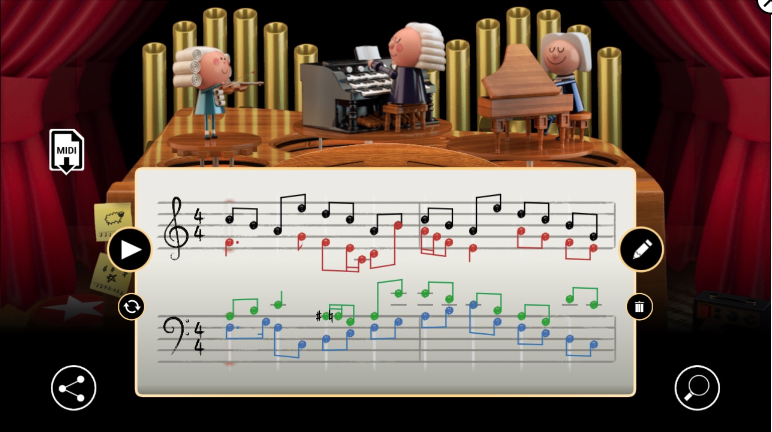
Figure 1: Example of chorale generation by Bach Doodle. The original soprano melody is in black and the generated counterpoint melodies in color (alto in red, tenor in green and bass in blue). © 2019, Google LLC, used with permission

As a further simplification, we consider only 4 measures long excerpts from the corpus. Therefore, the dataset is constructed by extracting all possible 4 measures long excerpts from the original 352 chorales, also transposed in all possible keys. Once trained on this dataset, the system may be used to generate three counterpoint voices corresponding to an arbitrary 4 measures long melody provided as an input. Somehow, it does capture the practice of Bach, who chose various melodies for a soprano voice and composed the three additional voices melodies (for alto, tenor and bass) in a counterpoint manner.

The input as well output representations are symbolic, of the piano roll type, with a direct encoding into one-hot vectors. Time quantization (the value of the time step) is set at the sixteenth note, which is the minimal note duration used in the corpus, i.e. there are 16 time steps for each 4/4 measure. The resulting input representation, which corresponds to the soprano melody, has the following size: 21 possible notes $\times$ 16 time steps $\times$ 4 measures = 1,344. The output representation, which corresponds to the concatenation of the three generated counterpoint melodies, has the following size: (21 + 21 + 28) $\times$ 16 $\times$ 4 = 4,480.

The architecture, shown in Figure 2, is feedforward (the most basic type of artificial neural network architecture) for a multiple classification task: to find out the most likely note for each time slice of the three counterpoint melodies. There is a single hidden layer with 200 units. Successive melody time slices are encoded into successive one-hot vectors which are concatenated and directly mapped to the input nodes. In Figure 2, each blackened vector element, as well as each corresponding blackened input node element, illustrate the specific encoding (one-hot vector index) of a specific note time slice, depending on its actual pitch (or a note hold in the case of a longer note, shown with a bracket). The dual process happens at the output. Each grey output node element illustrates the chosen note (the one with the highest probability), leading to a corresponding one-hot index, leading ultimately to a sequence of notes for each counterpoint voice. (For more details, see [3, Section 6.2.2].)

After training on several examples, generation can take place, with an example of chorale counterpoint generated from a soprano melody shown in Figure 3.

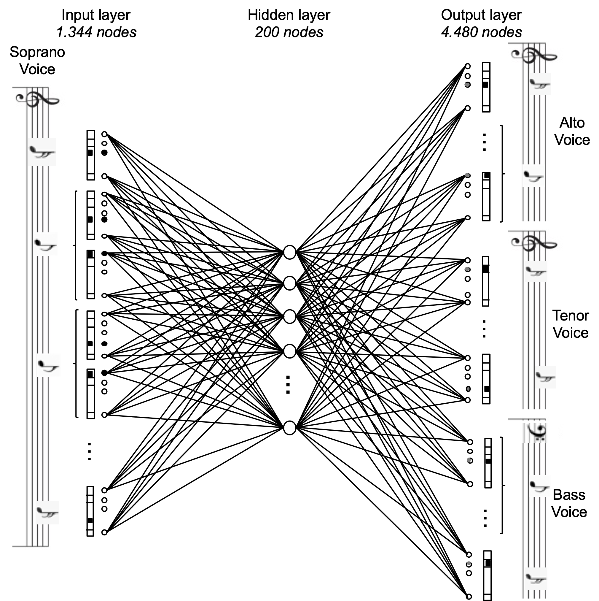
Figure 2: MiniBach architecture and encoding

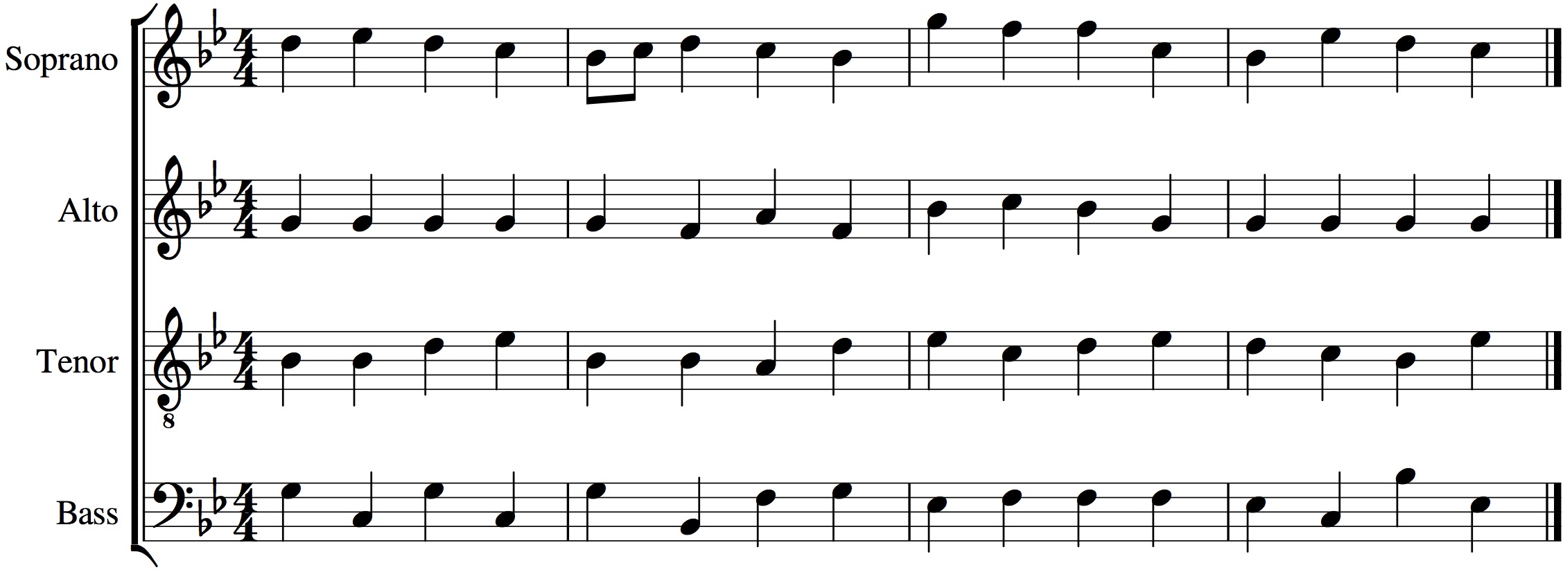
Figure 3: Example of a chorale counterpoint generated by MiniBach from a soprano melody

4 Pioneering Works and their Offsprings

As pointed out by Pons in [51], a first wave of applications of artificial neural networks to music appeared in the late 1980s. This corresponds to the second wave of the artificial neural networks movement [15, Section 1.2], with the innovation of hidden layer(s) and backpropagation [56, 40].

4.1 Todd’s Time-Windowed and Conditioned Recurrent Architectures

The experiments by Todd in [61] were one of the very first attempts at exploring how to use artificial neural networks to generate music. Although the architectures he proposed are not directly used nowadays, his experiments and discussion were pioneering and are still an important source of information.

Todd’s objective was to generate a monophonic melody in some iterative way. He named his first design the Time-Windowed architecture, shown in the left part of Figure 4, where a sliding window of successive time-periods of fixed size is considered (in practice, one measure long). Generation is conducted iteratively melody segment by segment (and recursively, as current output segment is entered as the next input segment and so on). Note that, although the network will learn the pairwise correlations between two successive melody segments, there is no explicit memory for learning long term correlations.

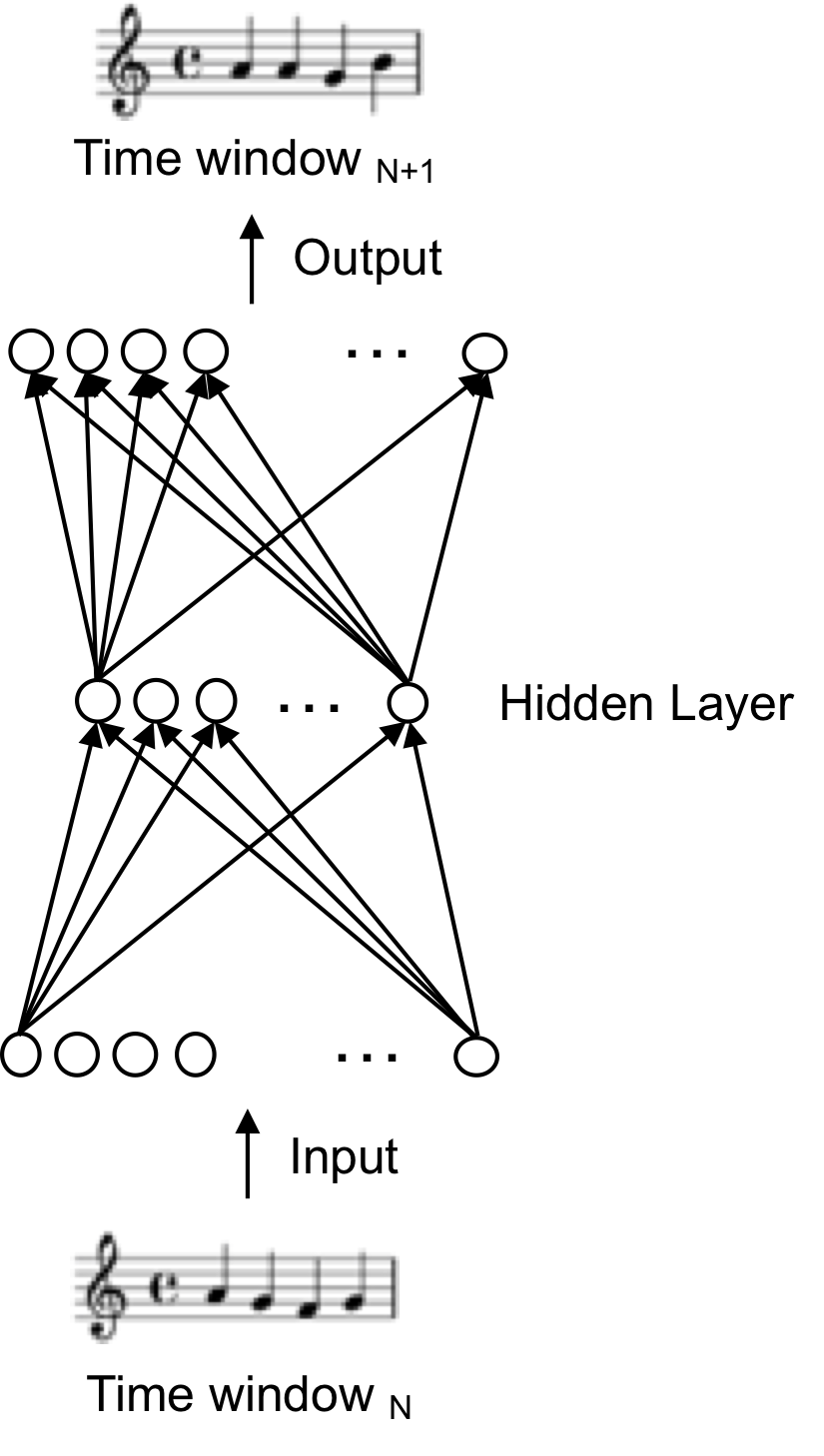
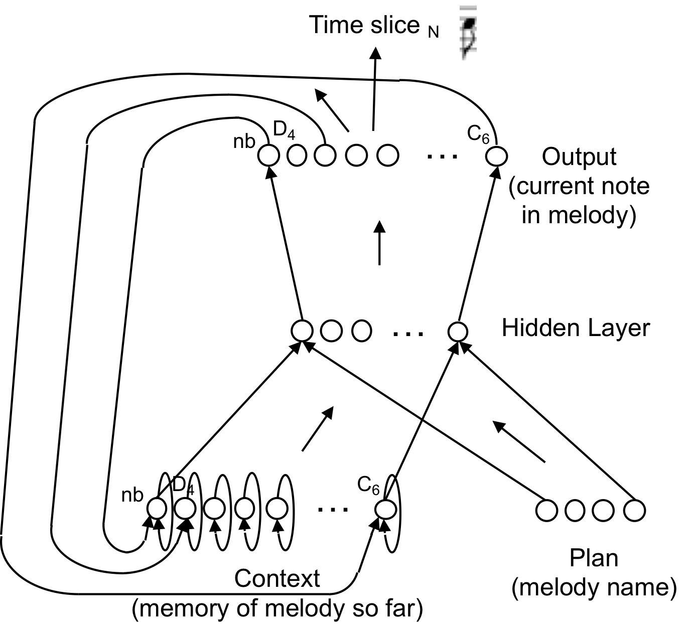
Figure 4: (left) Time-Windowed architecture. (right) Sequential architecture. Adapted from [61]

His third design is named Sequential and is shown in the right part of Figure 4. The input layer is divided in two parts, named the context and the plan. The context is the actual memory (of the melody generated so far) and consists in units corresponding to each note (D₄ to C₆), plus a unit about the note begin information (notated as “nb” in Figure 4). Therefore, it receives information from the output layer which produces next note, with a reentering connexion corresponding to each unit. In addition, as Todd explains it: “A memory of more than just the single previous output (note) is kept by having a self-feedback connection on each individual context unit.” The plan is a way to name a particular melody (among many) that the network has learnt.

Training is done by selecting a plan (melody) to be learnt. The activations of the context units are initialized to 0 in order to begin with a clean empty context. The network is then feedforwarded and its output, corresponding to the first time step note, is compared to the first time step note of the melody to be learnt, resulting in the adjustment of the weights. The output values are passed back to the current context. And then, the network is feedforwarded again, leading to the next time step note, again compared to the melody target, and so on until the last time step of the melody. This process is then repeated for various plans (melodies).

Generation of new melodies is conducted by feedforwarding the network with a new plan, corresponding to a new melody (not part of the training plans/melodies). The activations of the context units are initialized to 0 in order to begin with a clean empty context. Generation takes place iteratively, time step after time step. Note that, as opposed to the currently more common recursive generation strategy (to be detailed in Section 7.2.1), in which the output is explicitly reentered (recursively) into the input of the architecture, in Todd’s Sequential architecture the reentrance is implicit because of the specific nature of the recurrent connexions: the output is reentered into the context units while the input (the plan melody) is constant.

After having trained the network on a plan melody, various melodies may be generated by extrapolation by inputing new plans, or by interpolation between several (two or more) plans melodies that have been learnt. An example of interpolation is shown in Figure 5.

o_A)
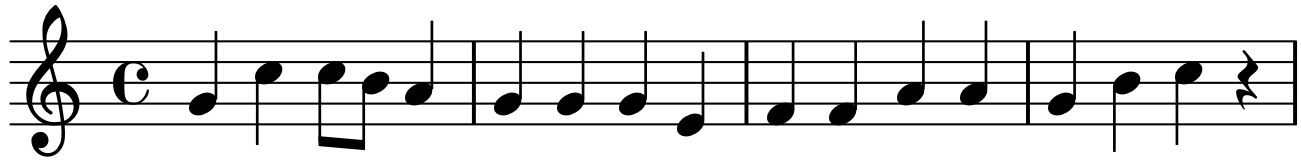
o_B)
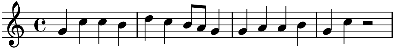
i₁)

Figure 5: Examples of melodies generated by the Sequential architecture. (o_A and o_B) Original plan melodies learnt. (i₁) Melody generated by interpolating between o_A plan and o_B plan melodies. Adapted from [61]

4.1.1 Influence

Todd’s Sequential architecture is one of the first examples of using a recurrent architecture and an iterative strategy for music generation. Moreover, note that introducing an extra input, named plan, which represents a melody that the network has learnt, could be seen as a precursor of conditioning architectures, where a specific additional input is used to condition (parametrize) the training of the architecture.

Furthermore, in the Addendum of the republication of his initial paper [62, pages 190–194], Todd mentions some issues and directions:

• structure and hierarchy – “One of the largest problems with this sequential network approach is the limited length of sequences that can be learned and the corresponding lack of global structure that new compositions exhibit. Hierarchically organized and connected sets of sequential networks hold promise for addressing these difficulties. (…) One solution to these problems is first to take the sequence to be learned and divide it up into appropriate chunks (…).”

• multiple time/clocks – “Of course, one way to present this subsequence-generating network with the appropriate sequence of plans is to generate those by another sequential network, operating at a slower time scale.”

Thus, these early designs may be seen as precursors of some recent proposals:

• hierarchical architectures, such as MusicVAE [53] (shown in Figure 6 and described in Section 9.3); and

• architectures with multiple time/clocks, such as Clockwork RNN [32] (shown in Figure 7) and SampleRNN [41].

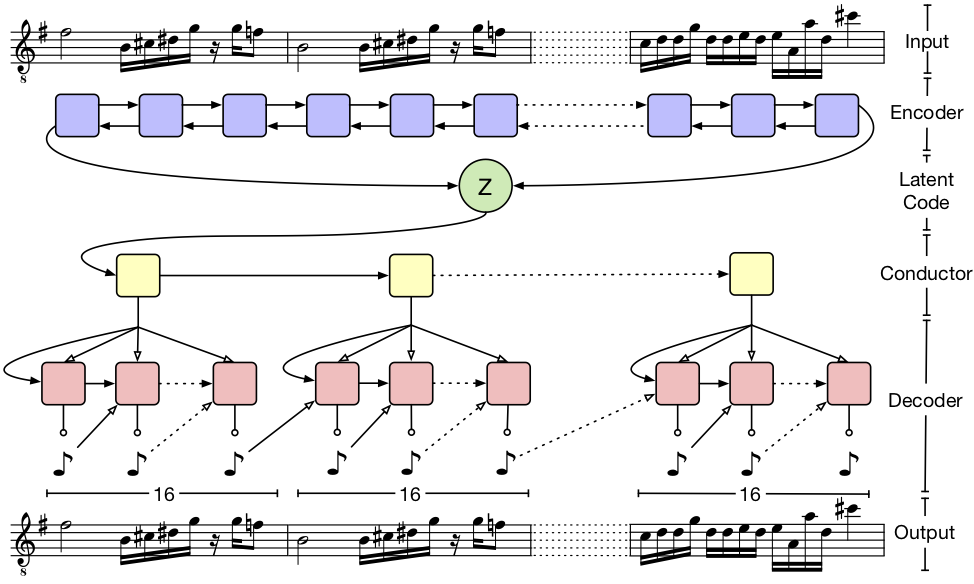
Figure 6: MusicVAE architecture. Reproduced from [53] with permission of the authors

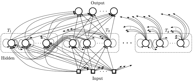
Figure 7: Clockwork RNN architecture. The RNN-like hidden layer is partitioned into several modules each with its own clock rate. Neurons in faster module $i$ are connected to neurons in a slower module $j$ only if a clock period $T_{i}<T_{j}$. Reproduced from [32] with permission of the authors

4.2 Lewis’ Creation by Refinement

In [35], Lewis introduced a novel way of creating melodies, that he named creation by refinement (CBR), by “reverting” the standard way of using gradient descent for the standard task – adjust the connexion weights to minimize the classification error –, into a very different task – adjust the input in order to make the classification output turn out positive.

In his described initial experiment [35], the architecture is a conventional feedforward neural network architecture used for binary classification, to classify “well-formed” melodies. The input is a 5-note melody, each note being among the 7 notes (from C to B, without alteration).

For the training phase, Lewis manually constructed 30 examples of what he meant by “well-formed” melodies: using only the following intervals between notes: unison, 3rd and 5th; and also following some scale degree stepwise motion (some training examples are shown in the left part of the Figure 8). He also constructed examples of poorly-formed melodies, not respecting the principles above. The training phase of the network is therefore conventional, by training it with the positive (well-formed) and negative examples that have been constructed.

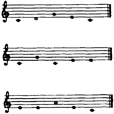
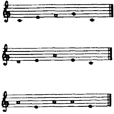
Figure 8: Creation by refinement. (left) Some “well formed” training examples. (right) Some examples of melodies generated. Reproduced from [35] with permission of the author. © 1988, IEEE, all rights reserved

For the creation by refinement phase, a vector of random values is produced, as values of the input nodes of the network. Then, a gradient descent optimization is applied iteratively to refine these values in order to maximize a positive classification (as shown in Figure 9). This will create a new melody which is classified as well-formed. The process may be done again, generating a new set of random values, and controlling their adjustment in order to create a new well-formed melody. The right part of Figure 8 shows some examples of generated melodies. Lewis interpretes the resulting creations as the fact that the network learned some preference for stepwise and triadic motion.

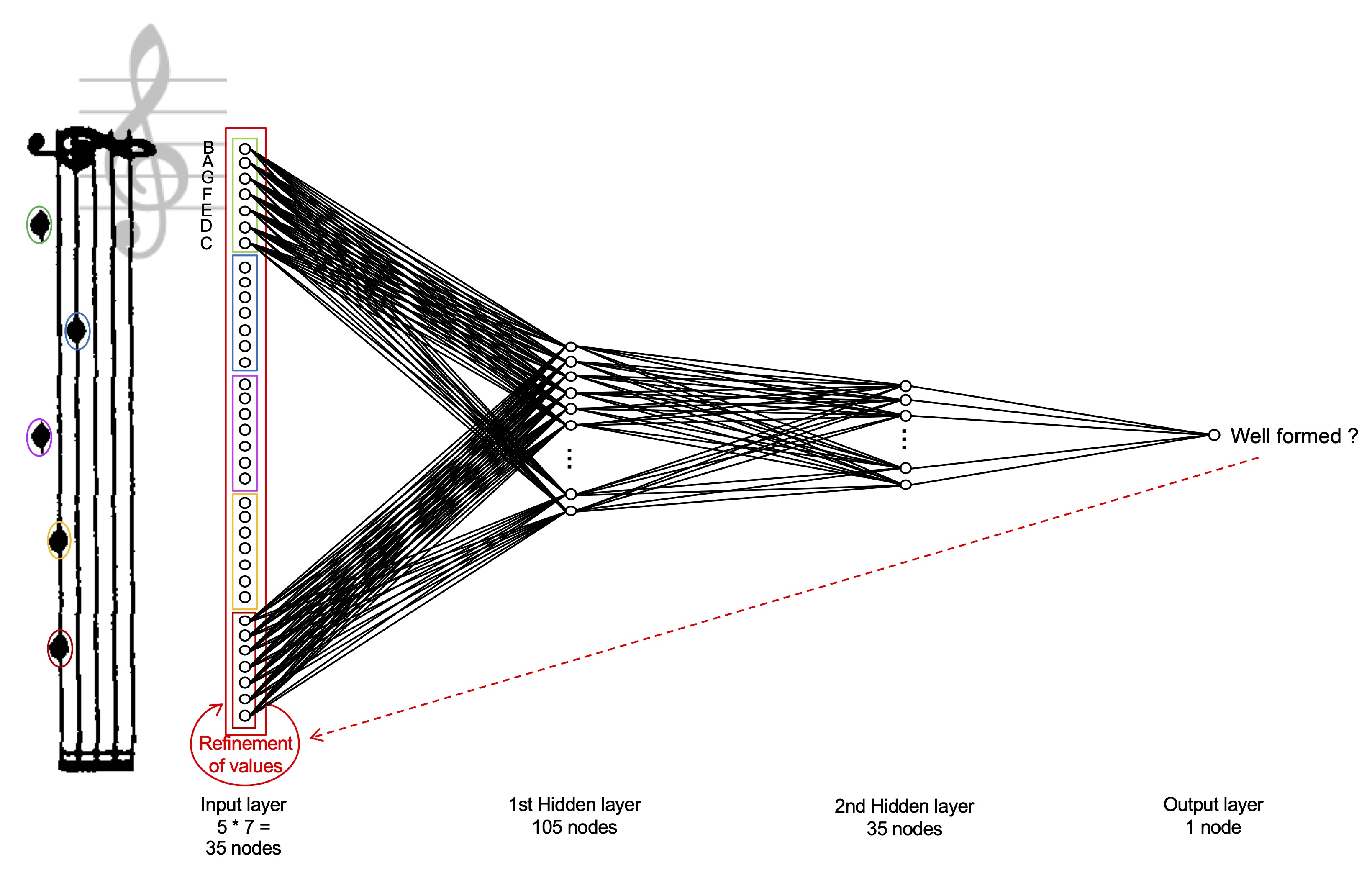
Figure 9: Creation by refinement – Architecture and strategy

4.2.1 Influence

The approach of creation by refinement by Lewis in 1988 can be seen as the precursor of various approaches for controlling the creation of a content by maximizing some target property. Examples of target properties are:

• maximizing a positive classification (as a well-formed melody), in Lewis’ original creation by refinement proposal [35];

• maximizing the similarity to a given target, in order to create a consonant melody, as in DeepHear [60];

• maximizing the activation of a specific unit, to amplify some visual element associated to this unit, as in Deep Dream [45];

• maximizing the content similarity to some initial image and the style similarity to a reference style image, to perform style transfer [14];

• maximizing the similarity of the structure to some reference music, to perform style imposition [34], as will be detailed in Section 9.6.

Interestingly, this is done by reusing standard training mechanisms, namely backpropagation to compute the gradients, as well as gradient descent (or ascent) to minimize the cost (or to maximize the objective).

Furthermore, in his extended article [36], Lewis proposed a mechanism of attention and also of hierarchy: “In order to partition a large problem into manageable subproblems, we need to provide both an attention mechanism to select subproblems to present to the network and a context mechanism to tie the resulting subpatterns together into a coherent whole.” and “The author’s experiments have employed hierarchical CBR. In this approach, a developing pattern is recursively filled in using a scheme somewhat analogous to a formal grammar rule such as ABC $\rightarrow$ AxByC. which expands the string without modifying existing tokens.”

The idea of an attention mechanism, although not yet very developed, may be seen as a precursor of attention mechanisms in deep learning architectures. It has initially been proposed as an additional mechanism to focus on elements of an input sequence during the training phase [15, Section 12.4.5.1], notably for language translation applications. More recently, it has been proposed as the fundamental and unique mechanism (as a full alternative to recurrence or to convolution) in the Transformer architecture [64], with its application to music generation, named MusicTransformer [28].

4.3 From Neural Networks to Deep Learning

Since the third wave of artificial neural networks, named deep learning, experiments on music generation are taking advantage of: huge processing power, optimized and standardized implementations (platforms), and availability of data, therefore allowing experiments at large or even very large scale. But, as we will see in Section 9, novel types of architectures have also been proposed. Before that, we will introduce a conceptual framework in order to help at organizing, analyzing and classifying the various types of architectures, as well as the various usages of artificial neural networks for music generation.

5 Conceptual Framework

This conceptual framework (initially proposed in [3]) is aimed at helping the analysis of the various perspectives (and elements) leading to the design of different deep learning-based music generation systems. It includes: five main dimensions (and their facets) to characterize different ways of applying deep learning techniques to generate musical content, and the associated typologies for each dimension. In this paper, we will simplify the presentation and focus on the most important aspects.

5.1 The 5 Dimensions

• Objective: the nature of the musical content to be generated, as well at its destination and use. Examples are: melody, polyphony, accompaniment; in the form of a musical score to be performed by some human musician(s) or an audio file to be played.

• Representation: the nature, format and encoding of the information (examples of music) used to train and to generate musical content. Examples are: waveform signal, transformed signal (e.g., a spectrum, via a Fourier transform), piano roll, MIDI, text; encoded in scalar variables or/and in one-hot vectors.

• Architecture: the nature of the assemblage of processing units (the artificial neurons) and their connexions. Examples are: feedforward, recurrent, autoencoder, generative adversarial networks (GAN).

• Requirement: one of the qualities that may be desired for music generation. Some are easier to achieve, e.g., content or length variability, and some other ones are deeper challenges [4], e.g., control, creativity or structure.

• Strategy: the way the architecture will process representations in order to generate the objective while matching desired requirements. Examples are: single-step feedforward, iterative feedforward, decoder feedforward, sampling, creation by refinement.

Note that these five dimensions are not completely orthogonal (unrelated). The exploration of these five different dimensions and of their interplay is actually at the core of our analysis.

5.2 The Basic Generation Steps

The basic steps for generating music, according to the objective, are as follows:

1. select (curate) a corpus (a set of training examples, representative of the style to be learnt);

2. select a type of representation and a type(s) of encoding and apply them to the examples;

3. select a type(s) of architecture and configurate it;

4. train the architecture with the examples;

5. select a type(s) of strategy for generation and apply it to generate one or various musical contents, and decode them into music;

6. select the preferred one(s) among the musics generated.

6 Representation

The choice of representation and its encoding is tightly connected to the configuration of the input and the output of the architecture, i.e. the number of input and output nodes (variables). Although a deep learning architecture can automatically extract significant features from the data, the choice of representation may be significant for the accuracy of the learning and for the quality of the generated content.

6.1 Phases and Types of Data

Before getting into the choices of representation to be processed by a deep learning architecture, it is important to identify the main types of data to be considered, depending on the phase (training or generation):

• training data, the examples used as input for the training;

• generation (input) data, used as input for the generation (e.g., a melody for which an accompaniment will be generated, as in the first example in Section 3); and

• generated (output) data, produced by the generation (e.g., the accompaniment generated), as specified by the objective.

Depending on the objective, these two types of data may be equal or different, e.g., in the example in Section 3, the generation data is a melody and the generated data is a set of (3) melodies.

6.2 Format

The format is the nature of the representation of a piece of music to be interpreted by a computer. A big divide in terms of the choice of representation is audio versus symbolic. This corresponds to the divide between continuous and discrete variables. Their respective raw material is very different in nature, as are the types of techniques for possible processing and transformation of the initial representation. However, the actual processing of these two main types of representation by a deep learning architecture is basically the same.

6.2.1 Audio

The main audio formats used are:

• signal waveform,

• spectrum, obtained via a Fourier transform.

The advantage of waveform is in considering the raw material untransformed, with its full initial resolution. Architectures that process the raw signal are sometimes named end-to-end architectures. The disadvantage is in the computational load: low level raw signal is demanding in terms of both memory and processing. The WaveNet architecture [47], used for speech generation for the Google assistants, was the first to prove the feasibility of such architectures.

6.2.2 Symbolic

The main symbolic formats used are:

• MIDI – It it is a technical standard that describes a protocol based on events, a digital interface and connectors for interoperability between various electronic musical instruments, softwares and devices [43]. Two types of MIDI event messages are considered for expressing note occurrence: Note on and Note off, to indicate, respectively, the start and the end of a note played. The MIDI note number, indicates the note pitch, specified by an integer within 0 and 127. Each note event is embedded into a data structure containing a delta-time value which also specifies the timing information, specified as a relative time (number of periodic ticks from the beginning – for musical scores) or as an absolute time (in the case of live performances).

• Piano roll – It is inspired from automated mechanical pianos with a continuous roll of paper with perforations (holes) punched into it. It is a two dimensional table with the x axis representing the successive time steps and the y axis the pitch, as shown in Figure 10.

• Text – A significant example is the ABC notation [65], a de facto standard for folk and traditional music. Each note is encoded as a token, the pitch class of a note being encoded as the letter corresponding to its English notation (e.g., A for A or La), with extra notations for the octave (e.g., a’ means two octaves up) and for the duration (e.g., A2 means a double duration). Measures are separated by “|” (bars), as in conventional scores. An example of ABC score is shown in Figure 11.

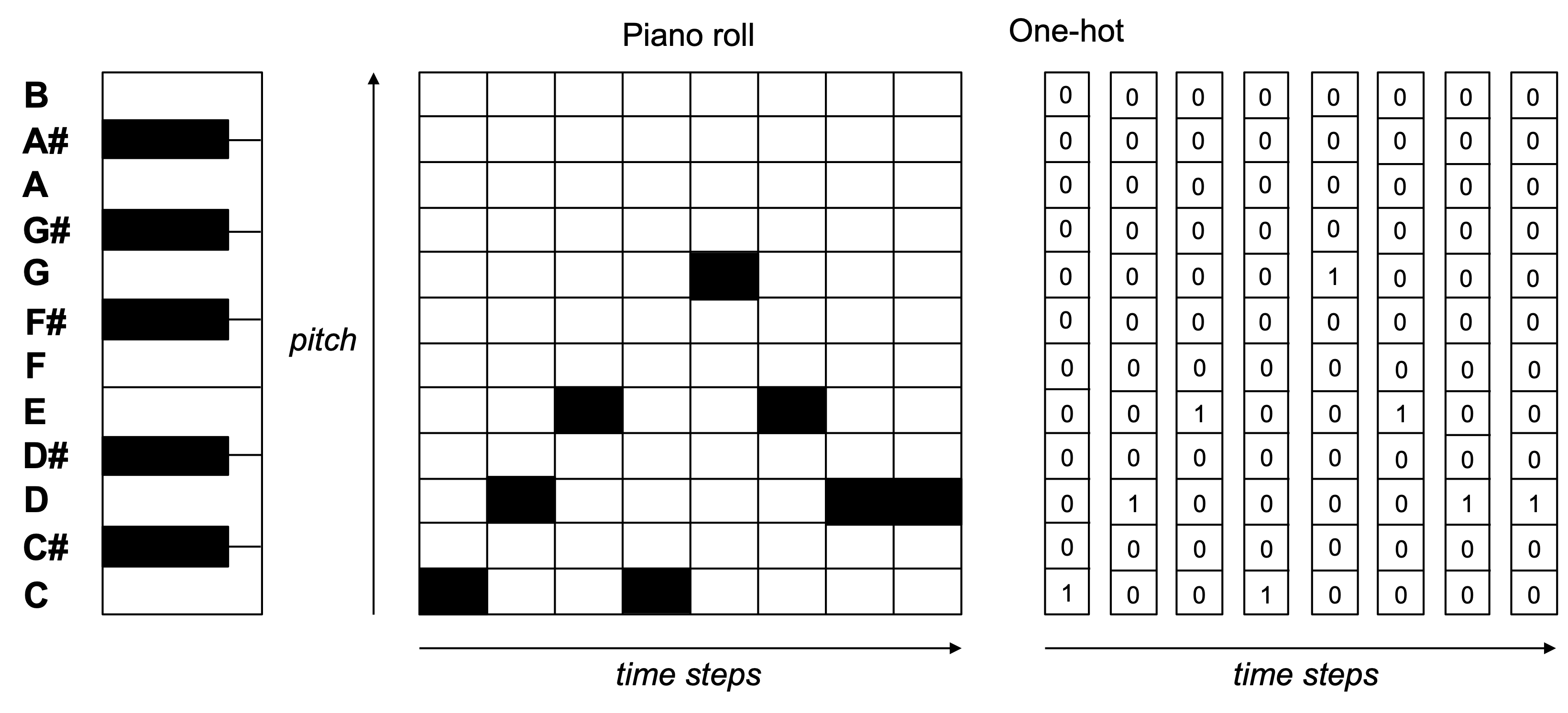
Figure 10: Example of piano roll and corresponding one-hot encoding

X: 1
T: A Cup Of Tea
R: reel
M: 4/4
L: 1/8
K: Amix
|:eA (3AAA g2 fg|eA (3AAA BGGf|eA (3AAA g2 fg|1afge d2 gf:
|2afge d2 cd|| |:eaag efgf|eaag edBd|eaag efge|afge dgfg:|

Figure 11: ABC notation of “A Cup of Tea”. The first six lines are the header and represent metadata: T(itle), M(eter), default note L(ength), K(ey), etc. Reproduced from The Session [30] with permission of the manager

Note that in these three cases, except for the case of live performances recorded in MIDI, a global time step has to be fixed and usually corresponds, as stated by Todd in [61], to the greatest common factor of the durations of all the notes to be considered.

Note that each format has its pros and cons. MIDI is probably the most versatile, as it can encompass the case of human interpretation of music (live performances), with arbitrary/expressive timing and dynamics of note events, as, e.g., used by the Performance RNN system [58]. But the start and the end of a long note will be represented into some very distant (temporal) positions, thus breaking the locality of information. The ABC notation is very compact but can only represent monophonic melodies. In practice, the piano roll is one of the most commonly used representations, although it has some limitations. An important one, compared to MIDI representation, is that there is no note off information. As a result, there is no way to distinguish between a long note and a repeated short note. Main possible approaches for resolving this are:

• to introduce a hold/replay representation, as a dual representation of the sequence of notes (as used in the DeepJ system [37]);

• to divide the size of the time step by two and always mark a note ending with a special tag (as used in [8]);

• to divide the size of the time step as in previous case, but instead mark a new note beginning (as used by Todd in [61], see Section 4.1); and

• to use a special hold symbol “__” in place of a note to specify when the previous note is held (as used in DeepBach [21], see Section 9.5).

The last solution, considering the hold symbol as a note, is simple and uniform but it only applies to the case of a monophonic melody.

6.3 Encoding

Once the format of a representation has been chosen, the issue still remains about how to encode this representation. The encoding of a representation (of a musical content) consists in the mapping of the representation (composed of a set of variables, e.g., pitch or dynamics) into a set of inputs (also named input nodes or input variables) for the neural network architecture.

There are two basic approaches:

• value-encoding – A continuous, discrete or boolean variable is directly encoded as a scalar; and

• one-hot-encoding – A discrete or a categorical variable is encoded as a categorical variable through a vector with the number of all possible elements as its length. Then, to represent a given element, the corresponding element of the one-hot vector is set to 1 and all other elements to 0.

For instance, the pitch of a note could be represented as a real number (its frequency in Hertz), an integer number (its MIDI note number), or a one-hot vector, as shown in the right part of Figure 10. The advantage of value encoding is its compact representation, at the cost of sensibility because of numerical operations (approximations). The advantage of one-hot encoding (actually the most common strategy) is its robustness against numerical operations approximations (discrete versus analog), at the cost of a high cardinality and therefore a potentially large number of nodes for the architecture.

7 Main Basic Architectures and Strategies

For reasons of space limitation, we will now jointly introduce architectures and strategies. For an alternative analysis guided by requirements (challenges), please see [4].

7.1 Feedforward Architecture

The feedforward architecture is the most basic and common type of artificial neural network architecture.

7.1.1 Feedforward Strategy

An example of use has been detailed in Section 3. The generation strategy used in this example is the most basic type of strategy, as it consists in feedforwarding within a single step the input data into the input layer, through successive hidden layers, until the output layer. Therefore we name it the single-step feedforward strategy, abbreviated as feedforward strategy.

7.1.2 Iterative Strategy

In Todd’s Time-Windowed architecture in Section 4.1, generation is processed iteratively by feedforwarding current melody segment in order to obtain next one, and so on. Therefore we name it the iterative feedforward strategy, abbreviated as iterative strategy.

7.2 Recurrent Architecture

A recurrent neural network (RNN) is a feedforward neural network extended with recurrent connexions in order to learn series of items (e.g., a melody as a sequence of notes). Todd’s Sequential architecture in Section 4.1 is an example although not of a common type. As pointed out in Section 4.1, in modern recurrent architectures, recurrent connexions are encapsulated within a (hidden) layer, which allows an arbitrary number of recurrent layers (as shown in Figure 12).

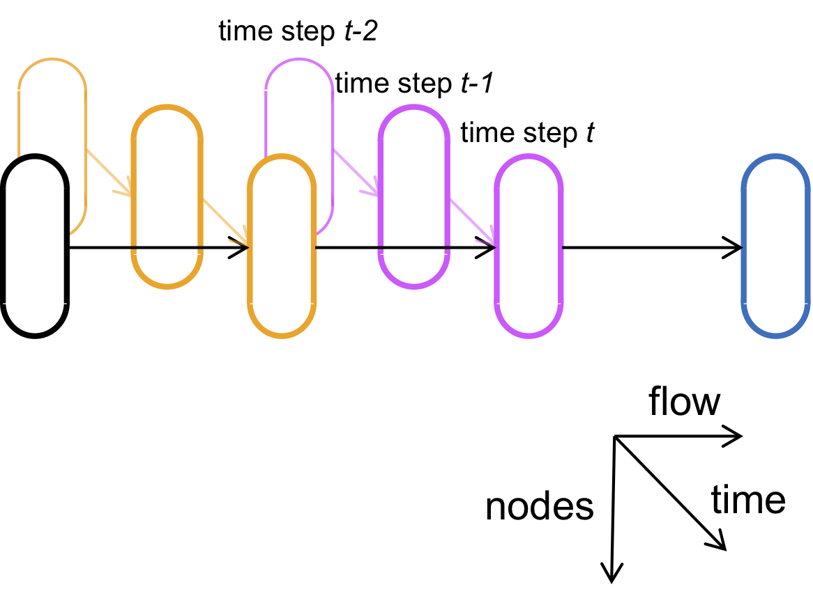
Figure 12: Recurrent neural network. Each successive layer (along the flow of computation) is represented as an oblong design (hiding the detail of its nodes). The diagonal axis represents the time dimension, with the previous step value of each layer in thinner and lighter color

7.2.1 Recursive Strategy

The first music generation experiment using current state of the art of recurrent architectures, the LSTM (Long Short-Term Memory [25]) architecture, is the generation of blues chord (and melody) sequences by Eck and Schmidhuber in [8]. Another interesting example is the architecture by Sturm et al. to generate Celtic melodies [59]. It is trained on examples selected from the folk music repository named The Session [30] and uses text (the ABC notation [65], see Section 6.2.2) as the representation format. Generation (an example is shown in Figure 13) is done using a recursive strategy, a special case of iterative strategy, for generating a sequence of notes (or/and chords), as initially described for text generation by Graves in [18]:

• select some seed information as the first item (e.g., the first note of a melody);

• feedforward it into the recurrent network in order to produce the next item (e.g., next note);

• use this next item as the next input to produce the next next item; and

• repeat this process iteratively until a sequence (e.g., of notes, i.e. a melody) of the desired length is produced.

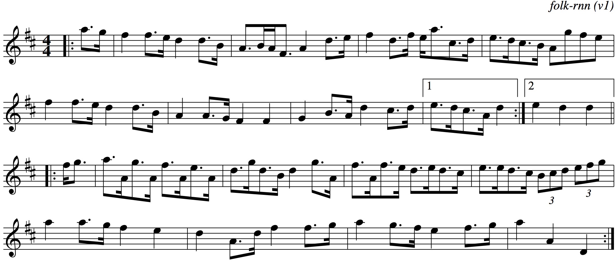
Figure 13: Score of “The Mal’s Copporim” automatically generated. Reproduced from [59] with permission of the authors

7.2.2 Sample Strategy

A limitation of applying straightforwardly the iterative feedforward strategy on a recurrent network is that generation is deterministic. As a consequence, feedforwarding the same input will always produce the same output. Indeed, as the generation of the next note, the next next note, etc., is deterministic, the same seed note will lead to the same generated series of notes. Moreover, as there are only 12 possible input values (the 12 pitch classes, disregarding the possible octaves), there are only 12 possible melodies.

Fortunately, the solution is quite simple. The assumption is that the generation is modeled as a classification task, i.e., the output representation of the melody is one-hot encoded and the output layer activation function is softmax. See an example in Figure 14, where $P(\text{x}_{t}=\text{C}|\text{x}_{<t})$ represents the conditional probability for the element (pitch of the note) x_t at step $t$ to be a C given the previous elements x_<t (the melody generated so far). The default deterministic strategy consists in choosing the pitch with the highest probability, i.e. $\text{argmax}_{\text{x}_{t}}P(\text{x}_{t}|\text{x}_{<t})$ (that is G$\sharp$ in Figure 14). We can then easily switch to a nondeterministic strategy, by sampling the output which corresponds (through the softmax function) to a probability distribution between possible pitches. By sampling a pitch following the distribution generated recursively by the architecture, we introduce stochasticity in the process of generation and thus content variability in the generation.

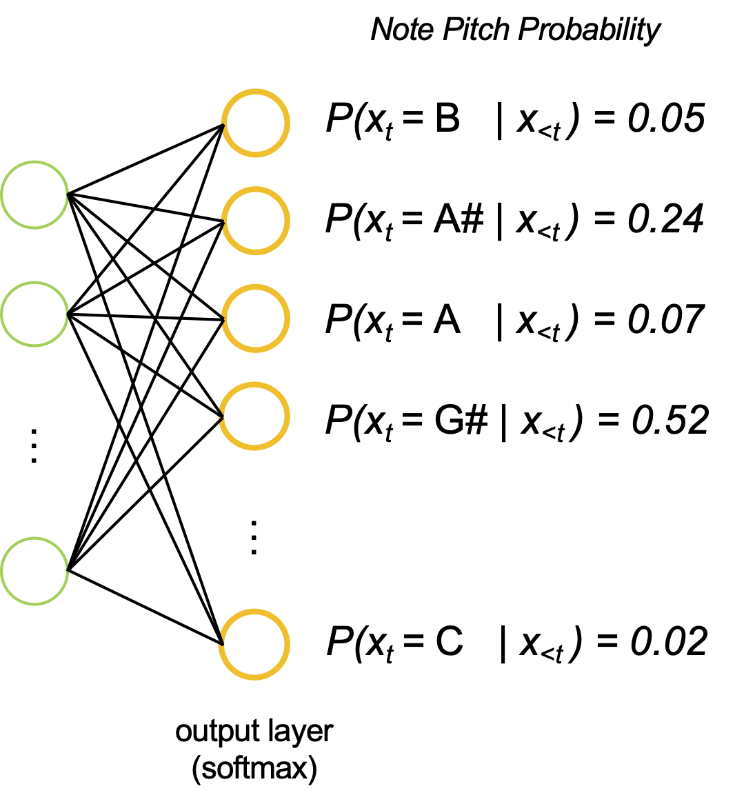
Figure 14: A softmax at the output layer computes the probability for each pitch

8 Compound Architectures

For more sophisticated objectives and requirements, compound architectures may be used. We will see that, from an architectural point of view, various types of combination may be used:

8.1 Composition

Several architectures, of the same type or of different types, are composed, e.g.:

• a bidirectional RNN, composing two RNNs, forward and backward in time, e.g., as used in the C-RNN-GAN [44] (see Figure 15) and the MusicVAE [53] (see Figure 6 and Section 9.3) architectures; and

• the RNN-RBM architecture [1], composing an RNN architecture and an RBM architecture.

8.2 Refinement

One architecture is refined and specialized through some additional constraint(s), e.g.:

• an autoencoder architecture (to be introduced in Section 9.1), which is a feedforward architecture with one hidden layer with the same cardinality (number of nodes) for the input layer and the output layer; and

• a variational autoencoder (VAE) architecture, which is an autoencoder with an additional constraint on the distribution of the variables of the hidden layer (see Section 9.2), e.g., the GLSR-VAE architecture [20].

8.3 Nesting

An architecture is nested into the other one, e.g.:

• a stacked autoencoder architecture, e.g., the DeepHear architecture [60]; and

• a recurrent autoencoder architecture (Section 9.3), where an RNN architecture is nested within an autoencoder, e.g., the MusicVAE architecture [53] (see Section 9.3).

8.4 Pattern

An architectural pattern is instantiated onto a given architecture(s), e.g.:

• the Anticipation-RNN architecture [19], that instantiates the conditioning pattern onto an RNN with the output of another RNN as the conditioning input; and

• the C-RNN-GAN architecture [44], where the GAN (Generative Adversarial Networks) pattern (to be introduced in Section 9.4) is instantiated onto two RNN architectures, the second one (discriminator) being bidirectional (see Figure 15); and

• the MidiNet architecture [67] (see Section 21), where the GAN pattern is instantiated onto two convolutional feedforward architectures, on which a conditional pattern is instantiated.

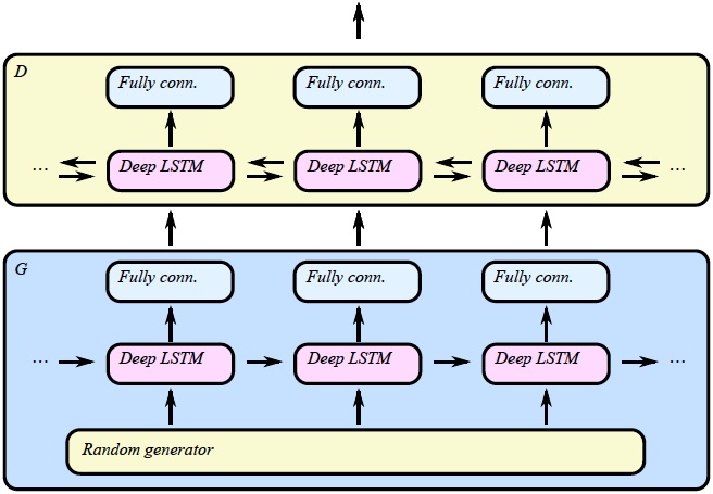
Figure 15: C-RNN-GAN architecture with the D(iscriminator) GAN component being a bidirectional RNN (LSTM). Reproduced from [44] with permission of the authors

8.5 Illustration

Figure 16 illustrates various examples of compound architectures and of actual music generation systems.

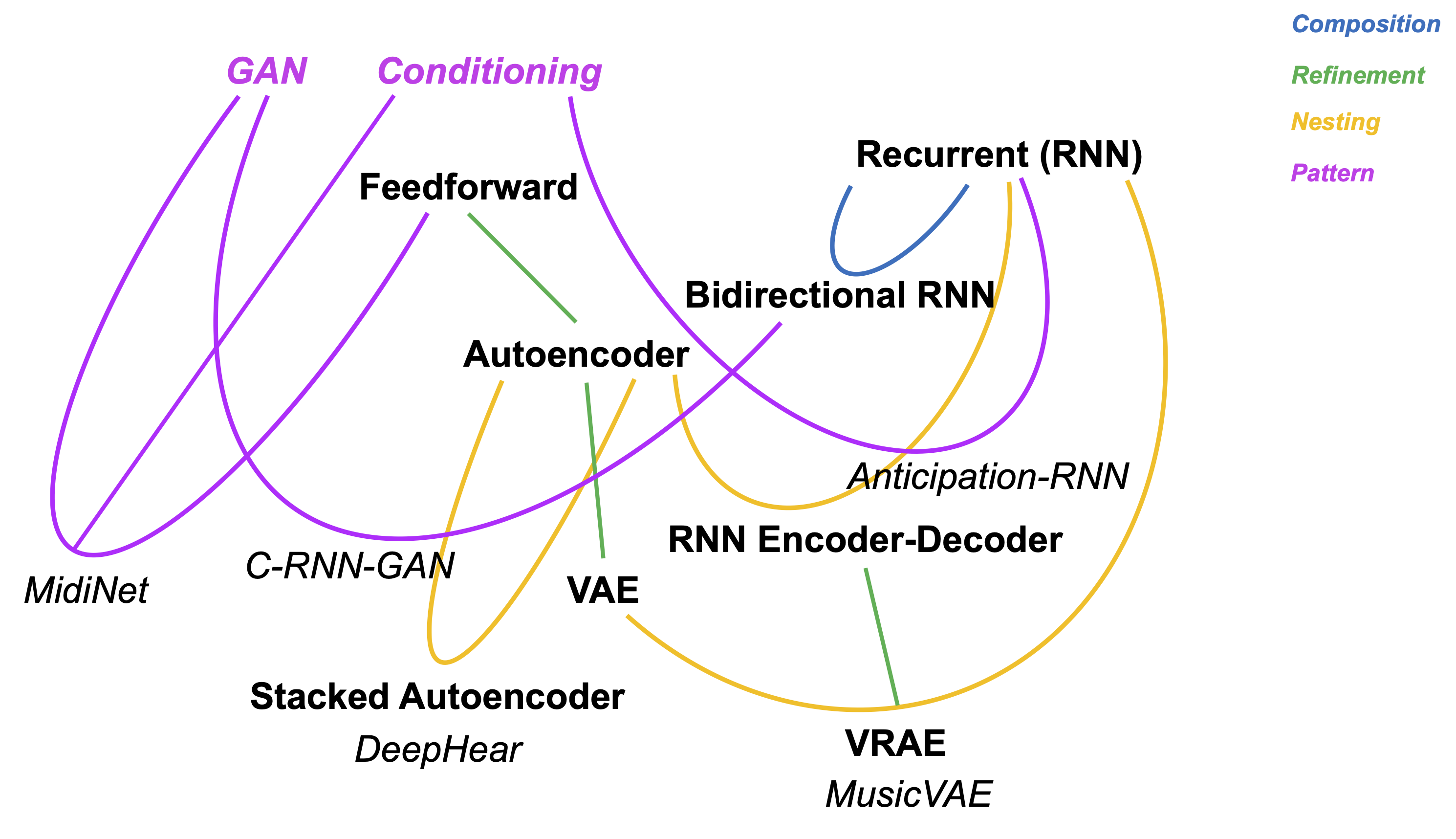
Figure 16: A tentative illustration of various examples and combination types (in color fonts) of compound architectures (in black bold font) and systems (in black italics font)

8.6 Combined Strategies

Note that the strategies for generation can be combined too, although not in the same way as the architectures: they are actually used simultaneously on different components of the architecture. In the examples discussed in Section 7.2.2, the recursive strategy is used by recursively feedforwarding current note into the architecture in order to produce next note and so on, while the sampling strategy is used at the output of the architecture to sample the actual note (pitch) from the possible notes with their respective probabilities.

9 Examples of Refined Architectures and Strategies

9.1 Autoencoder Architecture

An autoencoder is a refinement of a feedforward neural network with two constraints: (exactly) one hidden layer and the number of output nodes is equal to the number of input nodes. The output layer actually mirrors the input layer, creating its peculiar symmetric diabolo (or sand-timer) shape aspect, as shown in the left part of Figure 17.

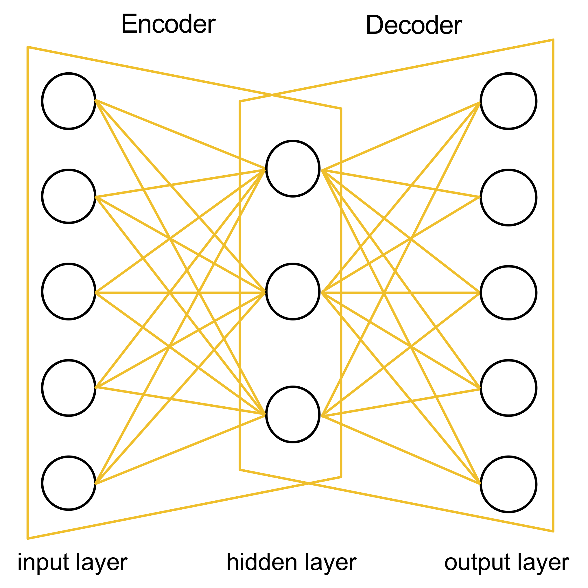
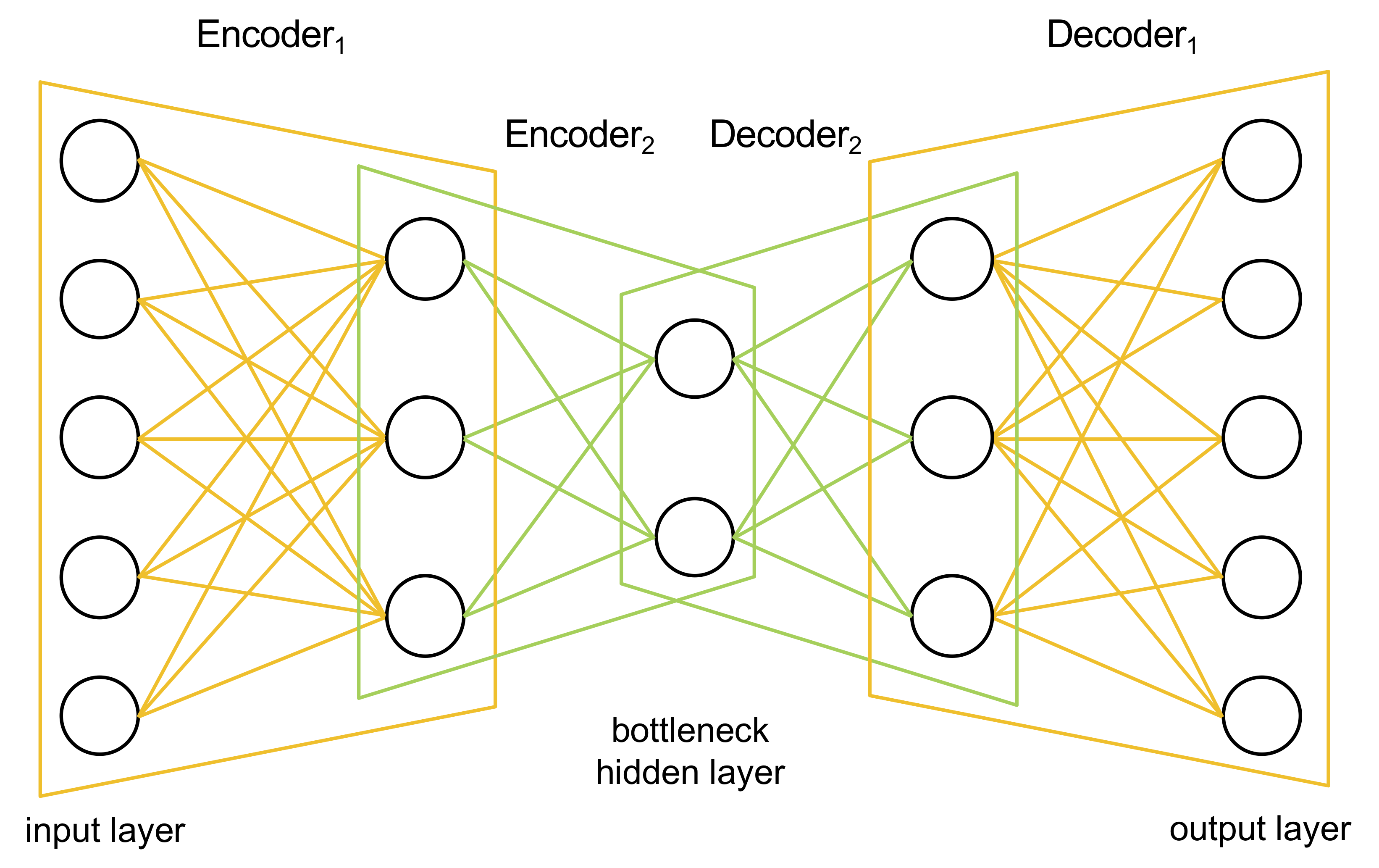
Figure 17: (left) Autoencoder architecture. (right) Stacked autoencoder (order-2) architecture

An autoencoder is trained with each of the examples as the input and as the output. Thus, the autoencoder tries to learn the identity function. As the hidden layer usually has fewer nodes than the input layer, the encoder component must compress information, while the decoder has to reconstruct, as accurately as possible, the initial information. This forces the autoencoder to discover significant (discriminating) features to encode useful information into the hidden layer nodes (also named the latent variables).

9.1.1 Decoder Feedforward Strategy

The latent variables of an autoencoder constitute a compact representation of the common features of the learnt examples. By instantiating these latent variables and decoding them (by feedforwarding them into the decoder), we can generate a new musical content corresponding to the values of the latent variables, in the same format as the training examples. We name this strategy the decoder feedforward strategy. An example generated after training an autoencoder on a set of Celtic melodies (selected from the folk music repository The Session [30], introduced in Section 7.2.1) is shown in Figure 18 (see [2] for more details). An early example of this strategy is the use of the DeepHear nested (stacked) autoencoder architecture to generate ragtime music according to the style learnt [60].

Figure 18: Example of melody generated by an autoencoder trained on a Celtic melodies corpus

9.2 Variational Autoencoder Architecture

Although producing interesting results, an autoencoder suffers from some discontinuity in the generation when exploring the latent space. A variational autoencoder (VAE) [31] is a refinement of an autoencoder where, instead of encoding an example as a single point, a variational autoencoder encodes it as a probability distribution over the latent space, from which the latent variables are sampled, and with the constraint that the distribution follows some prior probability distribution, usually a Gaussian distribution. This regularization ensures two main properties: continuity (two close points in the latent space should not give two completely different contents once decoded) and completeness (for a chosen distribution, a point sampled from the latent space should provide a “meaningful” content once decoded) [55]. The price to pay is some larger reconstruction error, but the tradeoff between reconstruction and regularity can be adjusted depending on the priorities.

As with an autoencoder, a VAE will learn the identity function, but furthermore the decoder will learn the relation between the prior (Gaussian) distribution of the latent variables and the learnt examples. A very interesting characteristic for generation purposes is therefore in the meaningful exploration of the latent space, as a variational autoencoder is able to learn a “smooth” mapping from the latent space to realistic examples [66].

9.2.1 Variational Generation

Examples of possible dimensions captured by latent variables learnt by the VAE are the note duration range (the distance between shortest and longest note) and the note pitch range (the distance between lowest and highest pitch). This latent representation (vector of latent variables) can be used to explore the latent space with various operations to control/vary the generation of content. Some examples of operations on the latent space (as summarized in [53]) are:

• translation;

• interpolation;

• averaging; and

• attribute vector arithmetics, by addition or subtraction of an attribute vector capturing a given characteristic.

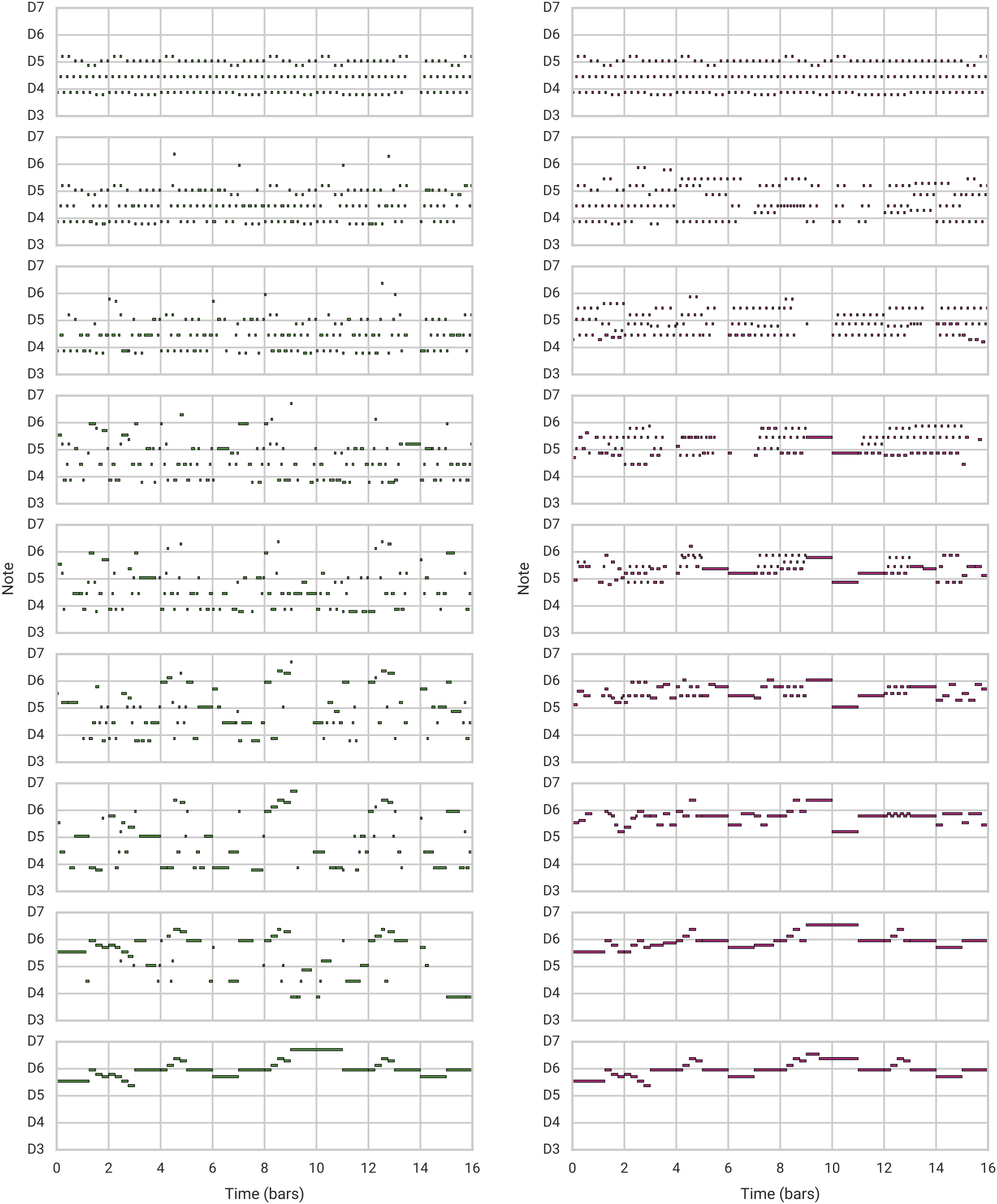
Figure 19: Comparison of interpolations between the top and the bottom melodies by (left) interpolating in the data (melody) space and (right) interpolating in the latent space and decoding it into melodies. Reproduced from [54] with permission of the authors

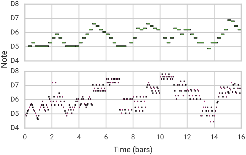
Figure 20: Example of a melody generated (bottom) by MusicVAE by adding a “high note density” attribute vector to the latent space of an existing melody (top). Reproduced from [54] with permission of the authors

9.2.2 Disentanglement

One limitation of using a variational autoencoder is that the dimensions (captured by latent variables) are not independent (orthogonal), as in the case of Principal component analysis (PCA). However, various techniques have being recently proposed to improve the disentanglement of the dimensions (see, e.g., [38]).

Another issue is that the semantics (meaning) of the dimensions captured by the latent variables is automatically “chosen” by the VAE architecture in function of the training examples and the configuration and thus can only be interpreted a posteriori. However, some recent approaches propose to “force” the meaning of latent variables, by splitting the decoder into various components and training them onto a specific dimension (e.g., rhythm or pitch melody) [68].

9.3 Variational Recurrent Autoencoder (VRAE) Architecture

An interesting example of nested architecture (see Section 8.3) is a variational recurrent autoencoder (VRAE). The motivation is to combine:

• the variational property of the VAE architecture for controlling the generation; and

• the arbitrary length property of the RNN architecture used with the recursive strategy.

An example (also hierarchical) is the MusicVAE architecture [53] (shown in Figure 6, with two examples of controlled generation in Figures 19 and 20).

9.4 Generative Adversarial Networks (GAN) Architecture

An interesting example of architectural pattern is the concept of Generative Adversarial Networks (GAN) [16], as illustrated in Figure 21. The idea is to simultaneously train two neural networks:

• a generative model (or generator) G, whose objective is to transform a random noise vector into a synthetic (faked) sample, which resembles real samples drawn from a distribution of real content (images, melodies…); and

• a discriminative model (or discriminator) D, which estimates the probability that a sample came from the real data rather than from the generator G.

The generator is then able to produce user-appealing synthetic samples from noise vectors.

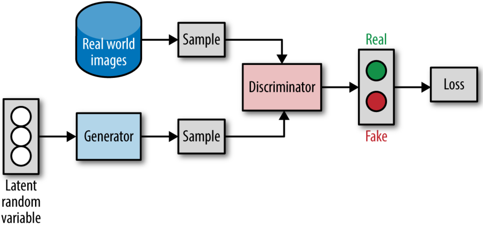
Figure 21: Generative adversarial networks (GAN) architecture. Reproduced from [52] with permission of O’Reilly Media

An example of the use of GAN for generating music is the MidiNet system [67], aimed at the generation of single or multitrack pop music melodies. The architecture, illustrated in Figure 22, follows two patterns: adversarial (GAN) and conditional (on history and on chords to condition melody generation). It is also convolutional (both the generator and the discriminator are convolutional networks). The representation chosen is obtained by transforming each channel of MIDI files into a one-hot encoding of 8 measures long piano roll representations. Generation takes place following an iterative strategy, by sampling one measure after one measure until reaching 8 measures. An example of generation is shown in Figure 23.

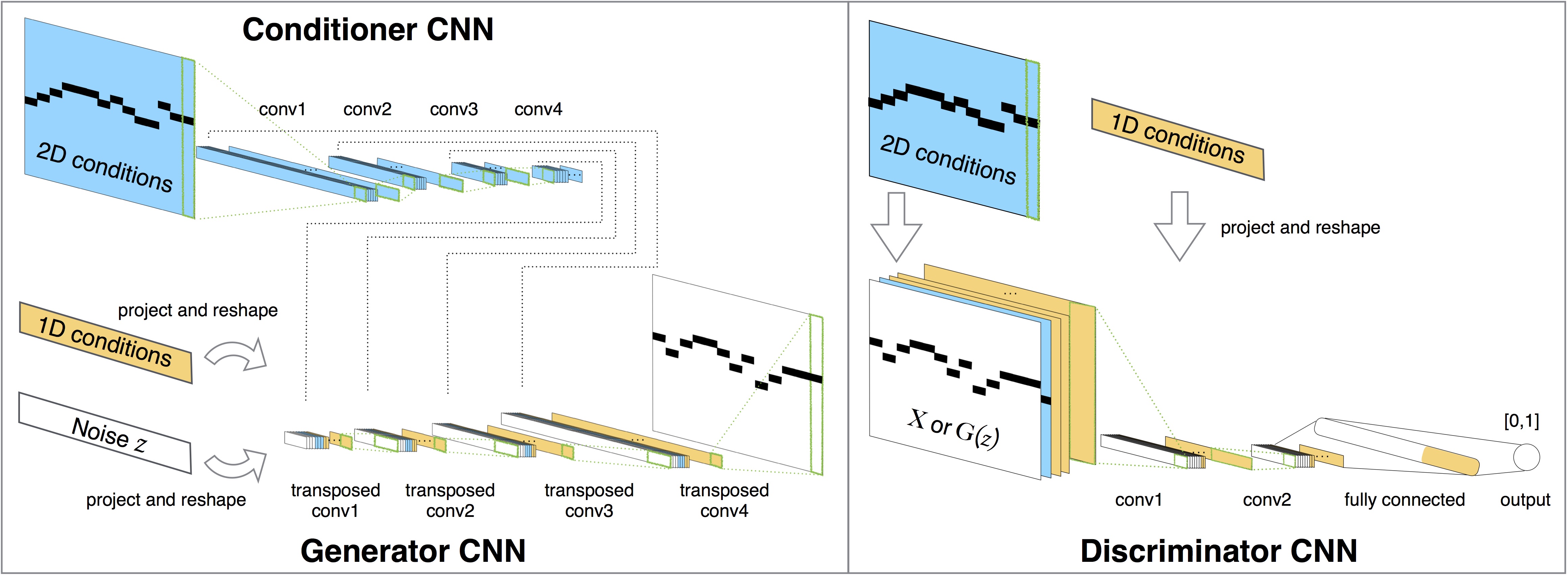
Figure 22: MidiNet architecture. Reproduced from [67] with permission of the authors

Figure 23: Example of melody and chords generated by MidiNet. Reproduced from [67] with permission of the authors

9.5 Sampling Strategy

We have discussed in the Section 7.2.2 the use of sampling at the output of a recurrent network in order to ensure content variability. But sampling could also be used as the principal strategy for generation, as we will see in the two following examples. The idea is to consider incremental variable instantiation, where a global representation is incrementally instantiated by progressively refining the values of variables (e.g., pitch and duration of notes). The main advantage is that it is possible to generate or to regenerate only an arbitrary part of the musical content, for a specific time interval and/or for a specific subset of tracks/voices, without having to regenerate the whole content.

This incremental instantiation strategy has been used in the DeepBach architecture [21] for generation of Bach chorales. The compound architecture, shown at Figure 24, combines two recurrent and two feedforward networks. As opposed to standard use of recurrent networks, where a single time direction is considered, DeepBach architecture considers the two directions forward in time and backward in time. Therefore, two recurrent networks (more precisely, LSTM) are used, one summing up past information and another summing up information coming from the future, together with a non recurrent network for notes occurring at the same time. Their three outputs are merged and passed as the input of a final feedforward neural network, whose output is the estimated distribution for all notes time slices for a given voice. The first 4 lines of the example data on top of the Figure 24 correspond to the 4 voices.

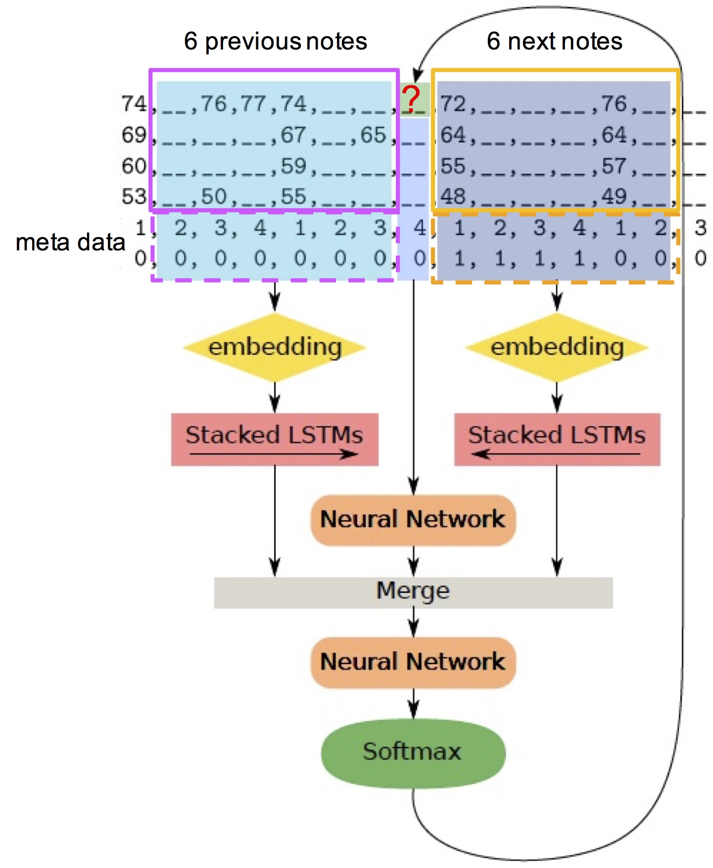
Figure 24: DeepBach architecture for the soprano voice prediction. Reproduced from [21] with permission of the authors

Training, as well as generation, is not done in the conventional way for neural networks. The objective is to predict the value of current note for a a given voice (shown with a red “?” on top center of Figure 24), using as information surrounding contextual notes. The training set is formed on-line by repeatedly randomly selecting a note in a voice from an example of the corpus and its surrounding context. Generation is done by sampling, using a pseudo-Gibbs sampling incremental and iterative algorithm (see details in [21]) to update values (each note) of a polyphony, following the distribution that the network has learnt.

The advantage of this method is that generation may be tailored. For example, if the user makes some local adjustment, he can resample only some of the corresponding counterpoint voices (e.g., alto and tenor) for the chosen interval (e.g., a measure and a half), as shown in Figure 25.

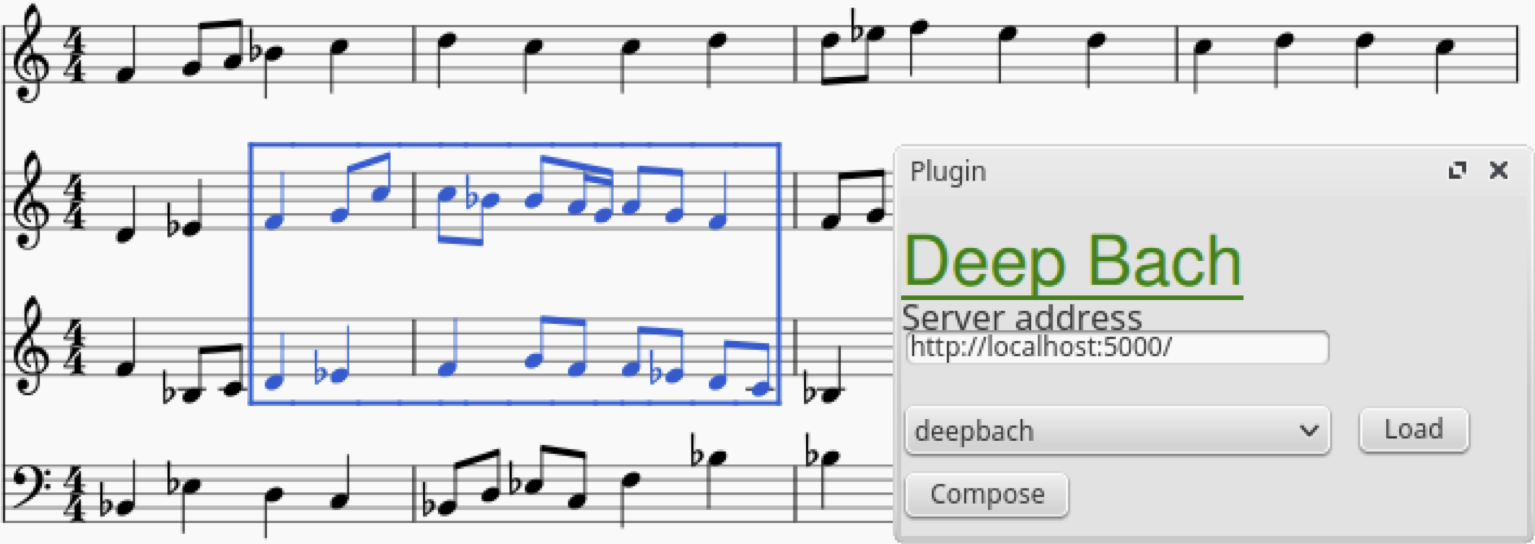
Figure 25: DeepBach user interface. Selecting an interval and two voices (alto and tenor) to be regenerated. Reproduced from [21] with permission of the authors

Coconet [27], the architecture used for implementing the Bach Doodle (introduced in Section 3), is another example of this approach. It uses a Block Gibbs sampling algorithm for generation and a different architecture (using masks to indicate for each time slice whether the pitch for that voice is known, see Figure 26). Please refer to [27] and [26] for details. An example of counterpoint accompaniment generation has been shown in Figure 1.

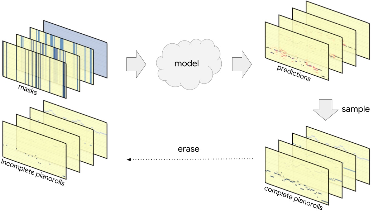
Figure 26: Coconet Architecture. Reproduced from [26] with permission of the authors

9.6 Creation by Refinement Strategy

Lewis’ creation by refinement strategy has been introduced in Section 4.2. It has been “reinvented” by various systems such as Deep Dream and DeepHear, as discussed in Section 4.2.1.

An example of application to music is the generation algorithm for the C-RBM architecture [34]. The architecture is a refined (convolutional) restricted Boltzmann machine (RBM). It is trained to learn the local structure (musical texture/style) of a corpus of music (in this case, Mozart sonatas). The main idea is to impose onto (and during) the creation of a new musical content some global structure seen as a structural template from an existing reference musical piece. The global structure is expressed through three types of constraints:

• self-similarity, to specify a global structure (e.g., AABA) in the generated music piece. This is modeled by minimizing the distance between the self-similarity matrices of the reference target and of the intermediate solution;

• tonality constraint, to specify a key (tonality). To control the key in a given temporal window, the distribution of pitch classes is compared with the key profiles of the reference; and

• meter constraint, to impose a specific meter (also named a time signature, e.g., 4/4) and its related rhythmic pattern (e.g., an accent on the third beat). The relative occurrence of note onsets within a measure is constrained to follow that of the reference.

Generation is performed via constrained sampling, a mechanism to restrict the set of possible solutions in the sampling process according to some pre-defined constraints. The principle of the process (illustrated at Figure 27) is as follows. At first, a sample is randomly initialized, following the standard uniform distribution. A step of constrained sampling is composed of $n$ runs of gradient descent (GD) to impose the high-level structure, followed by $p$ runs of selective Gibbs sampling (GS) to selectively realign the sample onto the learnt distribution. A simulated annealing algorithm is applied in order to control exploration to favor good solutions. Figure 28 shows an example of a generated sample in piano roll format.

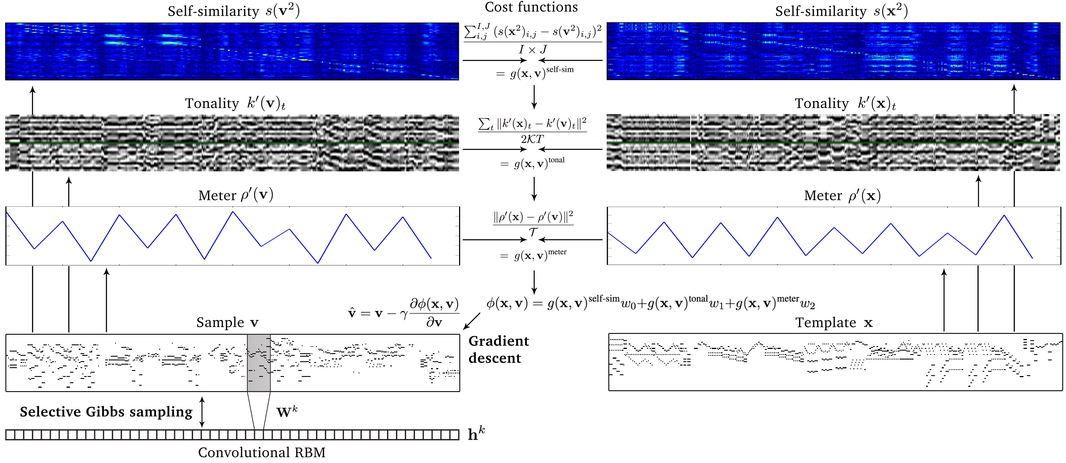
Figure 27: C-RBM Architecture generation algorithm. Reproduced from [34] with permission of the authors

Figure 28: Illustration of constrained sampling. Piano roll representation of: (top) Template piece, (middle) Intermediate sample after the GD phase, (bottom) Sample after the GS phase. Reproduced from [34] with permission of the authors

9.7 Other Architectures and Strategies

Researchers in the domain of deep learning techniques for music generation are designing and experimenting with various architectures and strategies, in most cases combinations or refinements of existing ones, or sometimes with novel types, as, e.g., in the case of MusicTransformer [28]. However, there is no guarantee that combining a maximal variety of types will make a sound and accurate architecture. Therefore, it is important to continue to deepen our understanding and to explore solutions as well as their possible articulations and combinations. We hope that this paper could contribute to that objective.

10 Open Issues and Trends

Because of space limitation, we will only sketch some of open issues and current trends about using neural networks and deep learning techniques for music generation. Following (and further developed in) [4], we consider some main challenges to be: control, structure, creativity and interactivity.

• Control is necessary to inject constraints (e.g., tonality, rhythm) in the generation, as witnessed by the C-RBM architecture (see Section 9.6). Some challenge is that a deep learning architecture is a kind of black box, therefore some control entry points (hooks) need to be identified, such as: the input (in the case of creation by refinement, as introduced in Section 4.2, or by using an extra conditioning input, as in Anticipation-RNN [19]); the output (in the case of constrained sampling, as in C-RBM); or an encapsulation (in the case of a reformulation through reinforcement learning, as in RL Tuner [29]).

• Structure is an important issue. Music generated by a deep learning architecture may be very pleasing for less than a minute but usually starts to be boring after a little while because of the absence of a clear sense of direction. Structure imposition is a first direction, as in C-RBM, or by using hierarchical architectures as in Music-VAE. A more ambitious direction is to favor the emergence of structure.

• Creativity is obviously a desired objective, while a difficult and profound issue. Neural networks are actually not well prepared, as their strength in generating music very conformant to a style learnt turns out to be a weakness for originality. Therefore, various strategies are being explored to try to favor exiting from the “comfort zone”, without losing it all. A notable attempt has been proposed for creating paintings in [9], by extending a GAN architecture to favor the generation of content difficult to classify within existing styles, and therefore favoring the emergence of new styles. Meanwhile, as discussed in Section 2.2, we believe that it is more interesting to use deep learning architectures to assist human musicians to create and construct music, than pursuing purely autonomous music generating systems.

• Therefore, interactivity is necessary to be able to allow a musician to incrementally develop a creation with the help of a deep learning-based system. This could be done, e.g., by allowing partial regeneration, as in [50], or by focusing on an incremental sampling strategy, as described in Section 9.5.

11 Conclusion

The use of artificial neural networks and deep learning architectures and techniques for the generation of music (as well as other artistic content) is a very active area of research. In this paper, we have: introduced the domain; analyzed early and pioneering proposals; and introduced a conceptual framework to help at analyzing and classifying the large diversity of architectures and experiments described in the literature, while illustrating it by various examples. We hope that this paper will help in better understanding the domain and trends of deep learning-based music generation.

Acknowledgements

This paper is dedicated to the memory of my beloved mother.

We thank Gaëtan Hadjeres and François Pachet for their participation to the book [3] which has been a significant initial input for this paper; CNRS, Sorbonne Université, UNIRIO and PUC-Rio for their support; and the various participants of our course on the topic for their feedback.

Annex – Glossary

Activation function

The function applied to the weighted sum for each neuron of a given layer. It is usually nonlinear (to introduce nonlinearity, in order to address the linear separability limitation of the Perceptron). Common examples are sigmoid or ReLU. The activation function of the output layer is a specific case (see Output layer activation function).

Algorithmic composition

The use of algorithms and computers to generate music compositions (symbolic form) or music pieces (audio form). Examples of models and algorithms are: grammars, rules, stochastic processes (e.g., Markov chains), evolutionary methods and artificial neural networks.

Architecture

An (artificial neural network) architecture is the structure of the organization of computational units (neurons), usually grouped in layers, and their weighted connexions. Examples of types of architecture are: feedforward (aka multilayer Perceptron), recurrent (RNN), autoencoder and generative adversarial networks (GAN). Architectures process encoded representations (in our case of a musical content).

Artificial neural network

A family of bio-inspired machine learning algorithms whose model is based on weighted connexions between computing units (neurons). Weights are incrementally adjusted during the training phase in order for the model to fit the data (training examples).

Attention mechanism

A mechanism inspired by the human visual system which focuses at each time step on some specific elements of the input sequence. This is modeled by weighted connexions onto the sequence elements (or onto the sequence of hidden units) which are subject to be learned.

Autoencoder

A specific case of artificial neural network architecture with an output layer mirroring the input layer and with one hidden layer. Autoencoders are good at extracting features.

Backpropagation

A short hand for “backpropagation of errors”, it is the algorithm used to compute the gradients of the cost function. Gradients will be used to guide the minimization of the cost function in order to fit the data.

Bias

The $b$ offset term of a simple linear regression model $h(\text{x})=b+\theta\text{x}$ and by extension of a neural network layer.

Bias node

The node of a neural network layer corresponding to a bias. Its constant value is 1 and is usually notated as $+1$.

Challenge

One of the qualities requirements that may be desired for music generation. Examples of challenges are: incrementality, originality and structure.

Classification

A machine learning task about the attribution of an instance to a class (from a set of possible classes). An example is to determine if next note is a C₄, a C$\sharp_{4}$, etc.

Compound architecture

An artificial neural network architecture which is the result of some combination of some architectures. Examples of types of combination are composition, nesting and pattern instantiation.

Conditioning architecture

The parametrization of an artificial neural network architecture by some conditioning information (e.g., a bass line, a chord progression…) represented via a specific extra input, in order to guide the generation.

Connexion

A relation between a neuron and another neuron representing a computational flow from the output of the first neuron to an input of the second neuron. A connexion is modulated by a weight which will be adjusted during the training phase.

Convolution

In mathematics, a mathematical operation on two functions sharing the same domain that produces a third function which is the integral (or the sum in the discrete case – the case of images made of pixels) of the pointwise multiplication of the two functions varying within the domain in an opposing way. Inspired both by mathematical convolution and by a model of human visions, it has been adapted to artificial neural networks and it improves pattern recognition accuracy by exploiting the spatial local correlation present in natural images. The basic principle is to slide a matrix (named a filter, a kernel or a feature detector) through the entire image (seen as the input matrix), and for each mapping position to compute the dot product of the filter with each mapped portion of the image and then sum up all elements of the resulting matrix.

Correlation

Any statistical relationship, whether causal or not, between two random variables. Artificial neural networks are good at extracting correlations between variables, for instance between input variables and output variables and also between input variables.

Cost function (aka Loss function)

The function used for measuring the difference between the prediction by an artificial neural network architecture (ŷ) and the actual target (true value y). Various cost functions may be used, depending on the task (prediction or classification) and the encoding of the output, e.g., mean squared error, binary cross-entropy and categorical cross entropy.

Counterpoint

In musical theory, an approach for the accompaniment of a melody through a set of other melodies (voices). An example is a chorale with 3 voices (alto, tenor and bass) matching a soprano melody. Counterpoint focuses on the horizontal relations between successive notes for each simultaneous melody (voice) and then considers the vertical relations between their progression (e.g., to avoid parallel fifths).

Creation by refinement strategy

A strategy for generating content based on the incremental modification of a representation to be processed by an artificial neural network architecture.

Cross-entropy

A function measuring the dissimilarity between two probability distributions. It is used as a cost (loss) function for a classification task to measure the difference between the prediction by an artificial neural network architecture (ŷ) and the actual target (true value y). There are two types of cross-entropy cost functions: binary cross-entropy when the classification is binary and categorical cross-entropy when the classification is multiclass with a single label to be selected.

Dataset

The set of examples used for training an artificial neural network architecture.

Decoder

The decoding component of an autoencoder which reconstructs the compressed representation (an embedding) from the hidden layer into a representation at the output layer as close as possible to the initial data representation at the input layer.

Decoder feedforward strategy

A strategy for generating content based on an autoencoder architecture in which values are assigned onto the latent variables of the hidden layer and forwarded into the decoder component of the architecture in order to generate a musical content corresponding to the abstract description inserted.

Deep learning (aka Deep neural networks)

An artificial neural network architecture with a significant number of successive layers.

Discriminator

The discriminative model component of generative adversarial networks (GAN) which estimates the probability that a sample came from the real data rather than from the generator.

Disentanglement

The objective of separating the different factors governing variability in the data (e.g., in the case of human images, identity of the individual and facial expression, in the case of music, note pitch range and note duration range).

Embedding

In mathematics, an injective and structure-preserving mapping. Initially used for natural language processing, it is now often used in deep learning as a general term for encoding a given representation into a vector representation.

Encoder

The encoding component of an autoencoder which transforms the data representation from the input layer into a compressed representation (an embedding) at the hidden layer.

Encoding

The encoding of a representation consists in the mapping of the representation (composed of a set of variables, e.g., pitch or dynamics) into a set of inputs (also named input nodes or input variables) for the neural network architecture. Examples of encoding strategies are: value encoding, one-hot encoding and many-hot encoding.

End-to-end architecture

An artificial neural network architecture that processes the raw unprocessed data – without any pre-processing, transformation of representation, or extraction of features – to produce a final output.

Feedforward

The basic way for a neural network architecture to process an input by feedforwarding the input data into the successive layers of neurons of the architecture until producing the output. A feedforward neural architecture (also named multilayer neural network or multilayer Perceptron, MLP) is composed of successive layers, with at least one hidden layer.

Fourier transform

A transformation (which could be continuous or discrete) of a signal into the decomposition into its elementary components (sinusoidal waveforms). As well as compressing the information, its role is fundamental for musical purposes as it reveals the harmonic components of the signal.

Generative adversarial networks (GAN)

A compound architecture composed of two component architectures, the generator and the discriminator, who are trained simultaneously with opposed objectives. The objective of the generator is to generate synthetic samples resembling real data while the objective of the discriminator is to detect synthetic samples.

Generator

The generative model component of generative adversarial networks (GAN) whose objective is to transform a random noise vector into a synthetic (faked) sample which resembles real samples drawn from a distribution of real data.

Gradient

A partial derivative of the cost function with respect to a weight parameter or a bias.

Gradient descent

A basic algorithm for training a linear regression model and an artificial neural network. It consists in an incremental update of the weight (and bias) parameters guided by the gradients of the cost function until reaching a minimum.

Harmony

In musical theory, a system for organizing simultaneous notes. Harmony focuses on the vertical relations between simultaneous notes, as objects on their own (chords), and then considers the horizontal relations between them (e.g., harmonic cadences).

Hidden layer

Any neuron layer located between the input layer and the output layer of a neural network architecture.

Hold

The information about a note that extends its duration over a single time step.

Hyperparameter

Higher-order parameters about the configuration of a neural network architecture and its behavior. Examples are: number of layers, number of neurons for each layer, learning rate and stride (for a convolutional architecture).

Input layer

The first layer of a neural network architecture. It is an interface consisting in a set of nodes without internal computation.

Iterative feedforward strategy

A strategy for generating content by generating its successive time slices.

Latent variable

In statistics, a variable which is not directly observed. In deep learning architectures, variables within a hidden layer. By sampling a latent variable(s), one may control the generation, e.g., in the case of a variational autoencoder.

Layer

A component of a neural network architecture composed of a set of neurons.

Linear regression

Regression for an assumed linear relationship between a scalar variable and one or several explanatory variable(s).

Linear separability

The ability to separate by a line or a hyperplane the elements of two different classes represented in an Euclidian space.

Long short-term memory (LSTM)

A type of recurrent neural network (RNN) architecture with capacity for learning long term correlations and not suffering from the vanishing or exploding gradient problem during the training phase (in backpropagation through time, recurrence brings repetitive multiplications which could lead to amplify numerical errors). The idea is to secure information in memory cells protected from the standard data flow of the recurrent network. Decisions about writing to, reading from and forgetting the values of cells are performed by the opening or closing of gates and are expressed at a distinct control level, while being learnt during the training process.

Many-hot encoding

Strategy used to encode simultaneously several values of a categorical variable, e.g., a triadic chord composed of three note pitches. As for a one-hot encoding, it is based on a vector having as its length the number of possible values (e.g., from C₄ to B₄). Each occurrence of a note is represented with a corresponding 1 with all other elements being 0.

Markov chain

A stochastic model describing a sequence of possible states. The chance to change from the current state to a state or to another state is governed by a probability and does not depend on previous states.

Melody

The abbreviation of a single-voice monophonic melody, that is a sequence of notes for a single instrument with at most one note at the same time.

Musical instrument digital interface (MIDI)

A technical standard that describes a protocol, a digital interface and connectors for interoperability between various electronic musical instruments, softwares and devices.

Multilayer Perceptron (MLP)

A feedforward neural architecture composed of successive layers, with at least one hidden layer. Also named Feedforward architecture.

Multivoice (aka Multitrack)

The abbreviation of a multivoice polyphony, that is a set of sequences of notes intended for more than one voice or instrument.

Neuron

The atomic processing element (unit) of an artificial neural network architecture. A neuron has several input connexions, each one with an associated weight, and one output. A neuron will compute the weighted sum of all its input values and then apply the activation function associated to its layer in order to compute its output value. Weights will be adjusted during the training phase of the neural network architecture.

Node

The atomic structural element of an artificial neural network architecture. A node could be a processing unit (a neuron) or a simple interface element for a value, e.g., in the case of the input layer or a bias node.

Objective

The nature and the destination of the musical content to be generated by a neural network architecture. Examples of objectives are: a monophonic melody to be played by a human flutist and a polyphonic accompaniment played by a synthesizer.

One-hot encoding

Strategy used to encode a categorical variable (e.g., a note pitch) as a vector having as its length the number of possible values (e.g., from C₄ to B₄). A given element (e.g., a note pitch) is represented with a corresponding 1 with all other elements being 0. The name comes from digital circuits, one-hot referring to a group of bits among which the only legal (possible) combinations of values are those with a single high (hot) (1) bit, all the others being low (0).

Output layer

The last layer of a neural network architecture.

Output layer activation function

The activation function of the output layer, which is usually: identity for a prediction task, sigmoid for a binary classification task and softmax for a multiclass single-label classification task.

Parameter

The parameters of an artificial neural network architecture are the weights associated to each connexion between neurons as well as the biases associated to each layer.

Perceptron

One of the first artificial neural network architecture, created by Rosenblatt in 1957. It had no hidden layer and suffered from the linear separability limitation.

Piano roll

Representation of a melody (monophonic or polyphonic) inspired from automated pianos. Each “perforation” represents a note control information, to trigger a given note. The length of the perforation corresponds to the duration of a note. In the other dimension, the localization (height) of a perforation corresponds to its pitch.

Pitch class

The name of the corresponding note (e.g., C) independently of the octave position. Also named chroma.

Polyphony

The abbreviation of a single-voice polyphony, that is a sequence of notes for a single instrument (e.g., a guitar or a piano) with possibly simultaneous notes.

Prediction

See regression.

Recurrent connexion

A connexion from an output of a node to its input. By extension, the recurrent connexion of a layer fully connects the outputs of all its nodes to all inputs of all its nodes. This is the basis of a recurrent neural network (RNN) architecture.

Recurrent neural network (RNN)

A type of artificial neural network architecture with recurrent connexions and memory. It is used to learn sequences.

Recursive feedforward strategy

A special case of iterative feedforward strategy where the current output is used as the next input.

Regression

In statistics, regression is an approach for modeling the relationship between a scalar variable and one or several explanatory variable(s).

Reinforcement learning

An area of machine learning concerned with an agent making successive decisions about an action in an environment while receiving a reward (reinforcement signal) after each action. The objective for the agent is to find the best policy maximizing its cumulated rewards.

Reinforcement strategy

A strategy for content generation by modeling generation of successive notes as a reinforcement learning problem while using an RNN as a reference for the modeling of the reward. Therefore, one may introduce arbitrary control objectives (e.g., adherence to current tonality, maximum number of repetitions, etc.) as additional reward terms.

ReLU

The rectified linear unit function, which may be used as a hidden layer nonlinear activation function, specially in the case of convolutions.

Representation

The nature and format of the information (data) used to train an architecture and to generate musical content. Examples of types of representation are: waveform signal, spectrum, piano roll and MIDI.

Requirement

One of the qualities that may be desired for music generation. Examples are: content variability, incrementality, originality and structure.

Rest

The information about the absence of a note (silence) during one (or more) time step(s).

Restricted Boltzmann machine (RBM)

A specific type of artificial neural network that can learn a probability distribution over its set of inputs. It is stochastic, has no distinction between input and output, and uses a specific learning algorithm.

Sampling

The action of producing an item (a sample) according to a given probability distribution over the possible values. As more and more samples are generated, their distribution should more closely approximate the given distribution.

Sampling strategy

A strategy for generating content where variables of a content representation are incrementally instantiated and refined according to a target probability distribution which has been previously learnt.

Seed-based generation

An approach to generate arbitrary content (e.g., a long melody) with a minimal (seed) information (e.g., a first note).

Sigmoid

Also named the logistic function, it is used as an output layer activation function for binary classification tasks and it may also be used as a hidden layer activation function.

Single-step feedforward strategy

A strategy for generating content where a feedforward architecture processes in a single processing step a global temporal scope representation which includes all time slices.

Softmax

Generalization of the sigmoid (logistic) function to the case of multiple classes. Used as an output layer activation function for multiclass single-label classification.

Spectrum

The representation of a sound in terms of the amount of vibration at each individual (as a function of) frequency. It is computed by a Fourier transformation which decomposes the original signal into its elementary (harmonic) components (sinusoidal waveforms).

Stacked autoencoder

A set of hierarchically nested autoencoders with decreasing numbers of hidden layer units.

Strategy

The way the architecture will process representations in order to generate the objective while matching desired requirements. Examples of types of strategy are: single-step feedforward, iterative feedforward and decoder feedforward.

Style transfer

The technique for capturing a style (e.g., of a given painting, by capturing the correlations between neurons for each layer) and applying it onto another content.

Time slice

The time interval considered as an atomic portion (grain) of the temporal representation used by an artificial neural network architecture.

Time step

The atomic increment of time considered by an artificial neural network architecture.

Turing test

Initially codified in 1950 by Alan Turing and named by him the “imitation game”, the “Turing test” is a test of the ability for a machine to exhibit intelligent behavior equivalent to (and more precisely, indistinguishable from) the behavior of a human. In his imaginary experimental setting, Turing proposed the test to be a natural language conversation between a human (the evaluator) and a hidden actor (another human or a machine). If the evaluator cannot reliably tell the machine from the human, the machine is said to have passed the test.

Unit

See neuron.

Variational autoencoder (VAE)

An autoencoder with the added constraint that the encoded representation (its latent variables) follows some prior probability distribution, usually a Gaussian distribution. The variational autoencoder is therefore able to learn a “smooth” latent space mapping to realistic examples which provides interesting ways to control the variation of the generation.

Value encoding

The direct encoding of a numerical value as a scalar.

Vanishing or exploding gradient problem

A known problem when training a recurrent neural network caused by the difficulty of estimating gradients, because, in backpropagation through time, recurrence brings repetitive multiplications and could thus lead to over amplify or minimize effects (numerical errors). The long short-term memory (LSTM) architecture solved the problem.

Waveform

The raw representation of a signal as the evolution of its amplitude in time.

Weight

A numerical parameter associated to a connexion between a node (neuron or not) and a unit (neuron). A neuron will compute the weighted sum of the activations of its connexions and then apply its associated activation function. Weights will be adjusted during the training phase.

References

- [1] Boulanger-Lewandowski, N., Bengio, Y., Vincent, P.: Modeling temporal dependencies in high-dimensional sequences: Application to polyphonic music generation and transcription. In: Proceedings of the 29th International Conference on Machine Learning (ICML-12), pp. 1159–1166. Edinburgh, Scotland, U.K. (2012)
- [2] Briot, J.P.: Compress to create. MusMat – Brazilian Journal of Music and Mathematics IV(1), 12–38 (2020)
- [3] Briot, J.P., Hadjeres, G., Pachet, F.D.: Deep Learning Techniques for Music Generation. Computational Synthesis and Creative Systems. Springer International Publishing (2019)
- [4] Briot, J.P., Pachet, F.: Music generation by deep learning: challenges and directions. Neural Computing and Applications (NCAA) 32(4), 981–993 (2020)
- [5] Cherry, E.C.: Some experiments on the recognition of speech, with one and two ears. The Journal of the Acoustical Society of America 25(5), 975–979 (1953)
- [6] Cope, D.: The Algorithmic Composer. A-R Editions (2000)
- [7] Dai, S., Zhang, Z., Xia, G.G.: Music style transfer issues: A position paper (2018). ArXiv:1803.06841v1
- [8] Eck, D., Schmidhuber, J.: A first look at music composition using LSTM recurrent neural networks. Tech. rep., IDSIA/USI-SUPSI, Manno, Switzerland (2002). No. IDSIA-07-02
- [9] Elgammal, A., Liu, B., Elhoseiny, M., Mazzone, M.: CAN: Creative adversarial networks generating “art” by learning about styles and deviating from style norms (2017). ArXiv:1706.07068v1
- [10] Emerging Technology from the arXiv: Deep learning machine solves the cocktail party problem. MIT Technology Review (2015). https://www.technologyreview.com/s/537101/deep-learning-machine-solves-the-cocktail-party-problem/
- [11] Fernández, J.D., Vico, F.: AI methods in algorithmic composition: A comprehensive survey. Journal of Artificial Intelligence Research (JAIR) (48), 513–582 (2013)
- [12] Fiebrink, R., Caramiaux, B.: The machine learning algorithm as creative musical tool (2016). ArXiv:1611.00379v1
- [13] Gamma, E., Helm, R., Johnson, R., Vlissides, J.: Design Patterns: Elements of Reusable Object-Oriented Software. Professional Computing Series. Addison-Wesley (1995)
- [14] Gatys, L.A., Ecker, A.S., Bethge, M.: A neural algorithm of artistic style (2015). ArXiv:1508.06576v2
- [15] Goodfellow, I., Bengio, Y., Courville, A.: Deep Learning. MIT Press (2016)
- [16] Goodfellow, I.J., Pouget-Abadie, J., Mirza, M., Xu, B., Warde-Farley, D., Ozairy, S., Courville, A., Bengio, Y.: Generative adversarial nets (2014). ArXiv:1406.2661v1
- [17] Google: Celebrating Johann Sebastian Bach (2019). https://www.google.com/doodles/celebrating-johann-sebastian-bach
- [18] Graves, A.: Generating sequences with recurrent neural networks (2014). ArXiv:1308.0850v5
- [19] Hadjeres, G., Nielsen, F.: Interactive music generation with positional constraints using Anticipation-RNN (2017). ArXiv:1709.06404v1
- [20] Hadjeres, G., Nielsen, F., Pachet, F.: GLSR-VAE: Geodesic latent space regularization for variational autoencoder architectures (2017). ArXiv:1707.04588v1
- [21] Hadjeres, G., Pachet, F., Nielsen, F.: DeepBach: a steerable model for Bach chorales generation (2017). ArXiv:1612.01010v2
- [22] Herremans, D., Chuan, C.H., Chew, E.: A functional taxonomy of music generation systems. ACM Computing Surveys (CSUR) 50(5) (2017)
- [23] Hiller, L.A., Isaacson, L.M.: Experimental Music: Composition with an Electronic Computer. McGraw-Hill (1959)
- [24] Hinton, G.E., Salakhutdinov, R.R.: Reducing the dimensionality of data with neural networks. Science 313(5786), 504–507 (2006)
- [25] Hochreiter, S., Schmidhuber, J.: Long short-term memory. Neural Computation 9(8), 1735–1780 (1997)
- [26] Huang, C.Z.A., Cooijmans, T., Dinculescu, M., Roberts, A., Hawthorne, C.: Coconet: the ML model behind today’s Bach Doodle (2019). https://magenta.tensorflow.org/coconet
- [27] Huang, C.Z.A., Cooijmans, T., Roberts, A., Courville, A., Eck, D.: Counterpoint by convolution. In: X. Hu, S.J. Cunningham, D. Turnbull, Z. Duan (eds.) Proceedings of the 18th International Society for Music Information Retrieval Conference (ISMIR 2017), pp. 211–218. ISMIR, Suzhou, China (2017)
- [28] Huang, C.Z.A., Vaswani, A., Uszkoreit, J., Shazeer, N., Hawthorne, I.S.C., Dai, A.M., Hoffman, M.D., Dinculescu, M., Eck, D.: Music Transformer: Generating music with long-term structure (2018). ArXiv:1809.04281v3
- [29] Jaques, N., Gu, S., Turner, R.E., Eck, D.: Tuning recurrent neural networks with reinforcement learning (2016). ArXiv:1611.02796v3
- [30] Keith, J.: The Session (Accessed on 21/12/2016). https://thesession.org
- [31] Kingma, D.P., Welling, M.: Auto-encoding variational Bayes (2014). ArXiv:1312.6114v10
- [32] Koutník, J., Greff, K., Gomez, F., Schmidhuber, J.: A clockwork RNN (2014). ArXiv:1402.3511v1
- [33] Krizhevsky, A., Sutskever, I., Hinton, G.E.: ImageNet classification with deep convolutional neural networks. In: Proceedings of the 25th International Conference on Neural Information Processing Systems, NIPS 2012, vol. 1, pp. 1097–1105. Curran Associates Inc., Lake Tahoe, NE, USA (2012)
- [34] Lattner, S., Grachten, M., Widmer, G.: Imposing higher-level structure in polyphonic music generation using convolutional restricted Boltzmann machines and constraints. Journal of Creative Music Systems (JCMS) 2(2) (2018)
- [35] Lewis, J.P.: Creation by refinement: A creativity paradigm for gradient descent learning networks. In: IEEE International Conference on Neural Networks, vol. II, pp. 229–233. San Diego, CA, USA (1988)
- [36] Lewis, J.P.: Creation by refinement and the problem of algorithmic music composition. In: P.M. Todd, D.G. Loy (eds.) Music and Connectionism, pp. 212–228. MIT Press (1991)
- [37] Mao, H.H., Shin, T., Cottrell, G.W.: DeepJ: Style-specific music generation (2018). ArXiv:1801.00887v1
- [38] Mathieu, E., Rainforth, T., Siddharth, N., Teh, Y.W.: Disentangling disentanglement in variational autoencoders (2019). ArXiv:1812.02833v3
- [39] Matisse, N.: How YACHT fed their old music to the machine and got a killer new album. ArsTechnica (2019). https://arstechnica.com/gaming/2019/08/yachts-chain-tripping-is-a-new-landmark-for-ai-music-an-album-that-doesnt-suck/
- [40] McClelland, J.L., Rumelhart, D.E., Group, P.R.: Parallel Distributed Processing – Explorations in the Microstructure of Cognition: Volume 2 Psychological and Biological Models. MIT Press (1986)
- [41] Mehri, S., Kumar, K., Gulrajani, I., Kumar, R., Jain, S., Sotelo, J., Courville, A., Bengio, Y.: SampleRNN: An unconditional end-to-end neural audio generation model (2017). ArXiv:1612.07837v2
- [42] Minsky, M., Papert, S.: Perceptrons: An Introduction to Computational Geometry. MIT Press (1969)
- [43] MMA: MIDI Specifications (Accessed on 14/04/2017). https://www.midi.org/specifications
- [44] Mogren, O.: C-RNN-GAN: Continuous recurrent neural networks with adversarial training (2016). ArXiv:1611.09904v1
- [45] Mordvintsev, A., Olah, C., Tyka, M.: Deep Dream (2015). https://research.googleblog.com/2015/06/inceptionism-going-deeper-into-neural.html
- [46] Nierhaus, G.: Algorithmic Composition: Paradigms of Automated Music Generation. Springer Nature (2009)
- [47] van den Oord, A., Dieleman, S., Zen, H., Simonyan, K., Vinyals, O., Graves, A., Kalchbrenner, N., Senior, A., Kavukcuoglu, K.: WaveNet: A generative model for raw audio (2016). ArXiv:1609.03499v2
- [48] Papadopoulos, A., Roy, P., Pachet, F.: Assisted lead sheet composition using FlowComposer. In: M. Rueher (ed.) Principles and Practice of Constraint Programming: 22nd International Conference, CP 2016, Toulouse, France, September 5-9, 2016, Proceedings, pp. 769–785. Springer Nature (2016)
- [49] Papadopoulos, G., Wiggins, G.: AI methods for algorithmic composition: A survey, a critical view and future prospects. In: AISB 1999 Symposium on Musical Creativity, pp. 110–117 (1999)
- [50] Pati, A., Lerch, A., Hadjeres, G.: Learning to traverse latent spaces for musical score inpainting (2019). ArXiv:1907.01164v1
- [51] Pons, J.: Neural networks for music: A journey through its history (2018). https://towardsdatascience.com/neural-networks-for-music-a-journey-through-its-history-91f93c3459fb
- [52] Ramsundar, B., Zadeh, R.B.: TensorFlow for Deep Learning. O’Reilly Media (2018)
- [53] Roberts, A., Engel, J., Raffel, C., Hawthorne, C., Eck, D.: A hierarchical latent vector model for learning long-term structure in music. In: Proceedings of the 35th International Conference on Machine Learning (ICML 2018). ACM, Montréal, PQ, Canada (2018)
- [54] Roberts, A., Engel, J., Raffel, C., Hawthorne, C., Eck, D.: A hierarchical latent vector model for learning long-term structure in music (2018). ArXiv:1803.05428v2
- [55] Rocca, J.: Understanding variational autoencoders (VAEs) – Building, step by step, the reasoning that leads to VAEs (2019). https://towardsdatascience.com/understanding-variational-autoencoders-vaes-f70510919f73
- [56] Rumelhart, D.E., McClelland, J.L., Group, P.R.: Parallel Distributed Processing – Explorations in the Microstructure of Cognition: Volume 1 Foundations. MIT Press (1986)
- [57] Shaw, M., Garlan, D.: Software Architecture: Perspectives on an Emerging Discipline. Prentice Hall (1996)
- [58] Simon, I., Oore, S.: Performance RNN: Generating music with expressive timing and dynamics (29/06/2017). https://magenta.tensorflow.org/performance-rnn
- [59] Sturm, B.L., Santos, J.F., Ben-Tal, O., Korshunova, I.: Music transcription modelling and composition using deep learning. In: Proceedings of the 1st Conference on Computer Simulation of Musical Creativity (CSCM 16). Huddersfield, U.K. (2016)
- [60] Sun, F.: DeepHear – Composing and harmonizing music with neural networks (Accessed on 21/12/2017). https://fephsun.github.io/2015/09/01/neural-music.html
- [61] Todd, P.M.: A connectionist approach to algorithmic composition. Computer Music Journal (CMJ) 13(4), 27–43 (1989)
- [62] Todd, P.M.: A connectionist approach to algorithmic composition. In: P.M. Todd, D.G. Loy (eds.) Music and Connectionism, pp. 190–194. MIT Press (1991)
- [63] Todd, P.M., Loy, D.G.: Music and Connectionism. MIT Press (1991)
- [64] Vaswani, A., Shazeer, N., Parmar, N., Uszkoreit, J., Jones, L., Gomez, A.N., Kaiser, L., Polosukhin, I.: Attention is all you need (2017). ArXiv:1706.03762v5
- [65] Walshaw, C.: abc notation home page (Accessed on 21/12/2016). http://abcnotation.com
- [66] Wild, C.M.: What a disentangled net we weave: Representation learning in VAEs (Pt. 1) (2018). https://towardsdatascience.com/what-a-disentangled-net-we-weave-representation-learning-in-vaes-pt-1-9e5dbc205bd1
- [67] Yang, L.C., Chou, S.Y., Yang, Y.H.: MidiNet: A convolutional generative adversarial network for symbolic-domain music generation. In: Proceedings of the 18th International Society for Music Information Retrieval Conference (ISMIR 2017). Suzhou, China (2017)
- [68] Yang, R., Wang, D., Wang, Z., Chen, T., Jiang, J., Xia, G.: Deep music analogy via latent representation disentanglement (2019). ArXiv:1906.03626v4