Numerical Simulations of the Molecular Behavior and Entropy of Non-Ideal Argon

Abstract

A numerical model is built, simulating the principles of kinetic gas theory, to predict pressures of molecules in a spherical pressure vessel; the model tracks a single particle and multiplies the force on the spherical walls by a mole of molecules to predict the net pressure. An intermolecular attractive force is added for high-density simulations, to replicate a real fluid; the force is chosen to ensure the fluid matches the Peng-Robinson equation of state as it is compressed to a near supercritical density. The standard deviations of the molecule position and velocity with respect to temperature and density is studied to define the entropy. A parametric study of a Stirling cycle heat engine utilizing near-supercritical densities is modeled, to study how the temperature dependence of the attractive intermolecular Van der Waal forces can affect the net total entropy change to the surrounding environment.

Email

mattdmarko@gmail.com

I Introduction

In the design of any thermodynamic system to convert heat to and from mechanical work, the laws of thermodynamics must always be considered. The first law of thermodynamics states that the change in internal energy equals the heat and work input into the working fluid ClausiusOrig ; 1 ; 2 ; 3 ; 4 ; StatThermo

$${{\delta}u} = {{\delta}q}-{{\delta}w},$$ (1)

where ${{\delta}u}$ (J/kg) is the change in specific internal energy, ${\delta}q$ (J/kg) is the specific heat transfered, and w (J/kg) is the specific work applied across the boundary 1 ; 2 ; 3 ; 4 ; StatThermo

$${\delta}w = {P}{\cdot}{{\delta}v}.$$ (2)

The second law has been described by Rudolph Clausius ClausiusOrig in 1854 as

$${{\oint}{\frac{{\delta}q}{T}}} \leq 0,$$ (3)

which states that any internally reversible thermodynamic cycle must generate a positive entropy ${\delta}s{\geq}0$ to the surrounding universe, where the change in entropy ${\delta}s$ (J/kg$\cdot$K) is defined as 1 ; 2 ; 3 ; 4 ; StatThermo ; Entropy01 ; Entropy02 ; Entropy03 ; Entropy04 ; Entropy05 ; Entropy06

$${\delta}{s} = \frac{{\delta}q}{T},$$ (4)

where T (K) is the absolute temperature, and ${\delta}q$ (J/kg) represent the heat transfered per unit mass. Because of Clausius’ equation, an ideal gas heat engine has a thermodynamic efficiency limit of the Carnot efficiency

$${\eta_{C}}={\frac{w_{out}}{q_{in}}}={\frac{{q_{in}}-{q_{out}}}{q_{in}}}={1-\frac{T_{L}}{T_{H}}},$$ (5)

though exceptions to equation 5 have been observed at the quantum level Carnot_PRL ; Carnot_PRX ; Carnot_NJOP as well as in the presence of supercritical fluids MarkoAIP .

Entropy is also defined as a level of disorder, characterized by Boltzmann’s entropy equation 1 ; 2 ; 3 ; 4

$$S={k_{B}}{\cdot}{log({\Omega})},$$ (6)

where S (J/K) represents the total entropy, $k_{B}$ (1.38065$\cdot$10^-23 J/K) represents Boltzmann’s constant, log represents the natural logarithm, and $\Omega$ represents the number of possible microstates of the system of molecules. If the molecules are at absolute zero (T = 0 K), when there is no movement of the molecules, then $\Omega$=1, and thus (according to equation 6) S=0 J/K.

Equation 6 can be derived from the equation for isothermal ($\delta{T}$=0) heating and expansion of an ideal gas. An ideal gas is a fluid at a low enough density where the intermolecular attractive and repulsive Van der Waal forces are negligible, and therefore the equation of state is defined in equation 7

$${{P}{\cdot}{V}} = {{N}{\cdot}{k_{B}}{\cdot}{T}},$$ (7)

where P (Pa) represents the pressure, V (m³) represents the total volume of the gas, N represents the number of molecules of the gas, ${k_{B}}$ is the Boltzmann constant (1.38065$\cdot$10^-23 J/K), and T (K) represents the absolute temperature. When an ideal gas is undergoing isothermal expansion 2 , the heat input $q_{{\delta}T=0}$ (J/kg) is equal to the work output $W_{{\delta}T=0}$ (J/kg) defined by equation 2, and therefore the heat input and work output of an ideal gas undergoing isothermal heating and expansion is defined in equation I

$${q_{{\delta}T=0}} = {W_{{\delta}T=0}}={\int}{P}{\cdot}{dV}={{N}{\cdot}{k_{B}}{\cdot}{T}{\cdot}{\int}{\frac{dV}{V}}},$$

$$= {N}{\cdot}{k_{B}}{\cdot}T{\cdot}log(\frac{V_{2}}{V_{1}}).$$

The change in entropy of an ideal gas is defined by equation 4, and therefore the change in entropy of an ideal gas undergoing isothermal expansion is found by plugging equation I into equation 4

$${{\delta}s_{{\delta}T=0}}=\frac{{\delta}q}{T}=N{\cdot}{k_{B}}{\cdot}log(\frac{V_{2}}{V_{1}})={k_{B}}{\cdot}log(\frac{V_{2}}{V_{1}})^{N}.$$ (9)

By doubling the volume, you are effectively doubling the number of microstates possible (for each molecule), and therefore one can derive equation 6 from 9.

II Kinetic Theory of an Ideal Gas

The kinetic model of an ideal gas 2 ; 3 ; KinTheoryBornGreen1946 is a well-established model to predict the kinetic energy of an ideal gas. Internal energy, by definition, is the summation of the kinetic energy from all of the random molecular motion within a fluid, as well as any potential energy from intermolecular forces. In the kinetic model, the gas is assumed to follow the ideal gas equation of state defined in equation 7. For the kinetic model to be applicable, the gas must be ideal, where all of the molecules are moving independent of each other, and there is no interaction between different gas molecules, either by collision or intermolecular forces 3 .

If a molecules is moving within the x direction and hits the boundary of a container or pressure vessel, provided the gas is thermodynamically stable and there is no heat transfer, it will bounce off of the wall in the opposite direction. The change in momentum for each molecular collision is therefore

$${\Delta}{p}=({{m_{m}}{\cdot}{v_{x}}})-({-{m_{m}}{\cdot}{v_{x}}})={2{\cdot}{m_{m}}{\cdot}{v_{x}}},$$ (10)

where ${\Delta}{p}$ (kg$\cdot$m/s) is the change in momentum, ${m_{m}}$ (kg) is the mass of an individual molecule, and $v_{x}$ is the velocity in the x-direction. The average time ${\Delta}{\tau}$ (s) for a molecule to cross the length L (m) of the pressure vessel is

$${\Delta}{\tau} = \frac{2{\cdot}L}{v_{x}}.$$ (11)

The force applied to the walls of the pressure vessel with an individual molecular collision $F_{m}$ (Newtons) is the change in momentum per unit time

$$F_{m}=\frac{{\Delta}{p}}{{\Delta}{\tau}}=\frac{{m_{m}}{\cdot}{v_{x}^{2}}}{L},$$ (12)

and the total force on the walls of the pressure vessel F (Newtons) is thus

$$F={N}{\cdot}{F_{m}}=\frac{{N}{\cdot}{m_{m}}{\cdot}{v_{x}^{2}}}{L},$$ (13)

where N is the total count of the molecules.

So far this analysis has only been in the x-direction, when in reality the molecules are bouncing in three dimensions. Assuming the average speed in all three directions are identical, as is the case in a stable fluid, according to Pythagorean theorem the average Root Mean Square (RMS) total velocity ${v_{RMS}}$ (m/s) is thus

$${v_{RMS}^{2}}={v_{x}^{2}}+{v_{y}^{2}}+{v_{z}^{2}}={3}{\cdot}{v_{x}^{2}},$$ (14)

and thus equation 13 can be rewritten as

$$F = \frac{{N}{\cdot}{m_{m}}{\cdot}{v_{RMS}^{2}}}{3{\cdot}L}.$$ (15)

In the kinetic theory, equation 15 would only apply to molecules that have no rotational or vibrational energies, specifically monatomic molecules such as helium, neon, argon, xenon, krypton, or radon gas 3 .

The pressure, by definition, is merely the ratio of the total force over the area of the container, and therefore assuming the container is cubic in shape, the pressure P (Pa) is

$$P=\frac{F}{L^{2}}=\frac{{N}{\cdot}{m_{m}}{\cdot}{v_{RMS}^{2}}}{3{\cdot}L^{3}}=\frac{{N}{\cdot}{m_{m}}{\cdot}{v_{RMS}^{2}}}{3{\cdot}V},$$ (16)

where V ($m^{3}$) is the volume of the container.

The total kinetic energy of the gas KE (J) is defined as the sum of the kinetic energies of the gas molecules

$$KE = {\frac{1}{2}}{\cdot}N{\cdot}{m_{m}}{\cdot}{v_{RMS}^{2}},$$ (17)

and therefore plugging equation 17 into equation 16

$$P = \frac{{2}{\cdot}{KE}}{3{\cdot}V},$$

and therefore the kinetic energy of a monatomic ideal gas can be defined as

$$KE = {\frac{3}{2}}{\cdot}{P}{\cdot}{V}.$$ (18)

As the kinetic model is dealing with an ideal gas, equation 7 is applicable, and thus 3

$$KE={\frac{3}{2}}{\cdot}{P}{\cdot}{V}={\frac{3}{2}}{\cdot}{m_{T}}{\cdot}{R}{\cdot}{T}={\frac{3}{2}}{\cdot}{N}{\cdot}{{k_{B}}}{\cdot}{T},$$ (19)

where $m_{T}$ (kg) is the total mass of the gas

$${m_{T}} = N{\cdot}{m_{m}}.$$

The relationship between temperature and kinetic energy is thus defined with equations 17 and 19. This can be rewritten as

$$KE={\frac{1}{2}}{\cdot}N{\cdot}{m_{m}}{\cdot}{v_{RMS}^{2}}={\frac{3}{2}}{\cdot}{N}{\cdot}{k_{B}}{\cdot}{T},$$

and thus the average total velocity of a particle of an ideal gas is proportional to the square root of the temperature 3

$$v_{RMS}=\sqrt{\frac{{3}{\cdot}{k_{B}}{\cdot}{T}}{m_{m}}}.$$ (20)

The kinetic heat energy ${\delta}q$ of a monatomic ideal gas is simply

$$U={\frac{3}{2}}{\cdot}{N}{\cdot}{k_{B}}{\cdot}{{\int}_{0}^{T}}{dT}={\frac{3}{2}}{\cdot}{N}{\cdot}{k_{B}}{\cdot}{T}.$$

The change in entropy of an ideal monatomic gas undergoing isochoric heating at a constant volume is therefore

$${\delta}s_{{\delta}V=0} = {{\frac{3}{2}}{\cdot}{N}{\cdot}{k_{B}}}{{\int}_{T_{0}}^{T}}{\frac{dT}{T}}={{\frac{3}{2}}{\cdot}{N}{\cdot}{k_{B}}}{\cdot}{log(\frac{T}{T_{0}})}$$ (21)

$$= {{\frac{3}{2}}{\cdot}{N}{\cdot}{k_{B}}}{\cdot}{log(\frac{{m_{m}}{\cdot}{v_{RMS}^{2}}/(3{\cdot}{k_{B}})}{{m_{m}}{\cdot}{v_{RMS,0}^{2}}/(3{\cdot}{k_{B}})})}$$

$$= {{\frac{3}{2}}{\cdot}{N}{\cdot}{k_{B}}}{\cdot}{log(\frac{v_{RMS}}{v_{RMS,0}})^{2}}$$

$$= {3}{\cdot}{N}{\cdot}{k_{B}}{\cdot}{log(\frac{v_{RMS}}{v_{RMS,0}})}$$

This represents the change in entropy for heating an ideal gas at a constant volume; it is different from equation 9, which represents the isothermal heating of an ideal gas with simultaneous expansion in order to maintain a constant temperature. If equation 9 and 21 are combined, the estimated entropy is

$$S = {N}{\cdot}{k_{B}}{\cdot}{\{{{3}{\cdot}log({v_{RMS}})}}+{log({\frac{V}{b{\cdot}MM}})}\}.$$ (22)

III Kinetic Gas Simulation

A model was build in the Fortran programming language, to simulate one mole (6.02214086${\cdot}{10^{23}}$) of argon molecules traveling in a spherical volume. Argon was chosen because it is a simple monatomic molecule, commonly used in industry, and its critical properties are not at excessively low temperatures (ex. Helium). Argon has a molar mass MM of 39.9 g/mole, a critical pressure $P_{c}$ of 4.863 MPa, a critical temperature ${T_{c}}$ of 150.687 K, a critical density of 535 kg/m², and a critical specific volume $V_{c}$ of 1.8692 cm³/g.

The model will take the dimensionless reduced temperature $T_{R}$ and reduced specific volume $V_{R}$ as inputs. The temperature is easily calculated as $T={T_{R}}{\cdot}{T_{c}}$, and the volume (for one mole) is calculated as ${V_{sphere}}={V_{R}}{\cdot}{V_{c}}{\cdot}{MM}$. From the known volume of the sphere, the radius and surface area are easily calculated as

$${R_{sphere}} = {({{\frac{3}{{\pi}{\cdot}4}}{\cdot}{V_{sphere}}})}^{\frac{1}{3}},$$ (23)

$${A_{sphere}} = {4}{\cdot}{\pi}{\cdot}{R_{sphere}^{2}},$$

The model has the option of simulating the particle at a constant speed for a given temperature, if so the speed is constantly the $v_{RMS}$ speed for the given temperature defined in equation 20. The model also gives the option of simulating a profile of faster and slower speeds; the speed profile will maintain the same RMS average speed defined in equation 20, and the average speed ${v_{avg}}$ (m/s) will be determined as

$${v_{avg}} = {v_{RMS}}{\cdot}{\sqrt{\frac{8}{3{\cdot}{\pi}}}}.$$ (24)

If the model calls for $N_{Y}$ velocity increments to be simulated, a subroutine in the Fortran code will generate a ${N_{Y}}{\cdot}{1}$ vector-array, ranging from 0.2 to 1.8, averaging 1.0, with a standard deviation of 0.71. This vector-array will be multiplied by the average molecule velocity at the boundary ${v_{avg}}$; the RMS of the velocity vector-array will be equal to ${v_{RMS}}$ determined with 20. Within this simulation, a value of $N_{Y}$ of 100 is used.

The time-step ${\delta}{\tau}$ (s) is determined by the estimated time for an argon molecule traveling at the average speed $v_{avg}$ (m/s) across the diameter of the sphere $2{\cdot}{R_{sphere}}$ (m). This time is divided by the integer value $N_{{\delta}{\tau}}$ that is specified by the model, to give a time-step.

$${{\delta}{\tau}}={({\frac{2{\cdot}{R_{sphere}}}{v_{avg}}})}{\cdot}{\frac{1}{N_{{\delta}{\tau}}}}$$ (25)

It is necessary to record the molecule’s position and velocity with each increment, but with different angles and speeds, it is impossible to know exactly how many time steps will be needed for each test parameter. In this Fortran code, an array length of ${10}{\cdot}{N_{{\delta}{\tau}}}$ was found to be more than enough to avoid any risk of running out of array space. In this study, a resolution of ${N_{{\delta}{\tau}}}$=300 was used; increasing the resolution beyond this number was not observed to have any significant impact on the results.

At each velocity increment, the model simulates a molecule leaving the surface of the sphere at different angles. As a sphere is effectively identical at all surface locations, the point of initial contact will be defined as (-R,0,0). The initial velocity will be defined in three dimensions as

$${V_{x}} = {V_{i}}{\cdot}{sin(\theta)}{\cdot}{cos(\phi)}$$ (26)

$${V_{y}} = {V_{i}}{\cdot}{sin(\theta)}{\cdot}{sin(\phi)}$$

$${V_{z}} = {V_{i}}{\cdot}{cos(\theta)},$$

where $\phi$ ranges from 0 to ${\pi}/2$, and $\theta$ ranges from 0 to $\pi$, both in 91 increments, resulting in 91²=8,281 different directions. The velocity magnitude $V_{i}$ (m/s) for the individual increment is determined from the temperature (equation 20), and $N_{Y}$=100; there is thus a total of 828,100 simulations for each temperature and volume increment.

The kinetic gas theory assumes the molecule travels across the long length of the volume and directly impacts the wall; in reality molecules will travel at all possible angles. If a molecule were to travel directly through the center of the sphere, the time ${\tau}$ (s) to travel will simply be ${\tau}={2{\cdot}{R_{sphere}/{v_{avg}}}}$, and the force due to the change in momentum for a single molecule will be derived from equation 15, where $F={{m_{m}}{\cdot}{v_{RMS}^{2}}}/({3{\cdot}2{\cdot}{R_{sphere}}})$. Assuming the spherical volume, if a molecule were to travel at an angle from the center of the sphere, the travel time $\tau$ (s) will be reduced, but the force will also be reduced as the molecule is hitting the surface at an angle, and will only transmit part of its energy to changing momentum and direction.

The simulation starts off with a molecule at position (-R,0,0). With each time-step, it increments the three dimensions based on the 3-dimensional velocity described in equation 26. The model uses a while loop until the radius ${r_{ii}}$ (m) of the position

$${r_{ii}} = \sqrt{{x^{2}}+{y^{2}}+{z^{2}}},$$ (27)

exceeds the radius of the sphere, ${r_{ii}}>{R_{sphere}}$. At this point, the molecule has impacted the cylinder wall. If the molecule travels right through the center and impacts the other end at position (R,0,0), then the velocity will be ${V_{i}}{\cdot}(1,0,0)$, and the force impacted will be at a maximum; the travel time $\tau$ (s) will also be the maximum ${\tau}={2{\cdot}{R_{sphere}/{V_{i}}}}$. If the molecule were to travel at a 90^∘ perpendicular direction, where the velocity were ${V_{i}}{\cdot}(0,1,0)$ or ${V_{i}}{\cdot}(0,0,1)$, the position will remain at (-R,0,0) and the travel time $\tau$ will effectively be 0. For all the molecules traveling at angles in between the two extremes, the force applied is simply the dot product of the velocity with the position of the impact

$$VX_{rat} = {{X_{x}}{\cdot}{V_{x}}}+{{X_{y}}{\cdot}{V_{y}}}+{{X_{z}}{\cdot}{V_{z}}},$$ (28)

and the dimensionless $VX_{rat}$ is applied to the equation for the force applied by a single molecule ${F_{m}}$ (N) defined in equation 29

$${F_{m}} = \frac{{VX_{rat}}{\cdot}{m_{m}}{\cdot}{\sqrt{{V_{x}^{2}}+{V_{y}^{2}}+{V_{z}^{2}}}}}{{3{\cdot}2{\cdot}{R_{sphere}}}}.$$ (29)

Throughout this simulation, for all initial angles and velocities, the position and velocity in three dimensions is tabulated and recorded. Each position and velocity is stored in a large data file, and at the conclusion of the simulation, the average, RMS, and standard deviation of both the positions and the velocities are determine. The purpose of determining the standard deviation is to find the relationship between the standard deviation of the position and velocity, as it relates to entropy, determined with equations 4, 9, and 21.

IV Kinetic-Potential Simulation

The ideal gas equation breaks down in the presence of intermolecular attractive and repulsive Van der Waal forces, and therefore empirical equations of states are used, such as the Redlich-Kwong RK1949 and the Peng-Robinson equation of state PR1976 ; PitzerAcentric

$${P} = {\frac{R{\cdot}T}{v-B}}-{\frac{A{\cdot}{\alpha}}{{v^{2}}+{2{\cdot}B{\cdot}v}-{B^{2}}}},$$ (30)

$$A = 0.45724{\cdot}{\frac{{R^{2}}{\cdot}{T_{c}^{2}}}{P_{c}}},$$

$$B = 0.07780{\cdot}{\frac{R{\cdot}{T_{c}}}{P_{c}}},$$

$${\alpha} = {({1+{{\kappa}{\cdot}{({1-{\sqrt{T_{R}}}})}}})^{2}},$$

$${\kappa} = {0.37464}+{1.54226{\cdot}{\omega}}-{0.26992{\cdot}{\omega^{2}}},$$

where $\omega$ is Pitzer’s acentric factor, defined as

$${\omega} = log_{10}(\frac{P_{c}}{P_{S}^{\prime}})-1,$$ (31)

where $P_{S}^{\prime}$ (Pa) is the saturated pressure at a reduced temperature of $T_{R}=0.7$, and $P_{c}$ (Pa) is the critical pressure. For all of the monatomic fluids including argon, ${\omega}=0$. The coefficient A represents the intermolecular attractive force, and the coefficient B represents the actual volume of the molecules at absolute zero. As the specific volume v (m³/kg) increases (and the density decreases), equation 30 matches the ideal gas law defined in equation 7.

As the density of a fluid increases to the point of being a saturated liquid, saturated gas, or supercritical fluid, intermolecular attractive (and repulsive) forces KeesomOrig ; Keesom2 ; LondonDispOrig ; IntermolCermanic ; RS_DispersionTemp ; TempDepPhysRevB can impact the pressure and temperature of the fluid. As the molecules get closer togetehr in the presence of attractive intermolecular forces, the internal potential energy will decrease. The thermodynamic data yields an empirical equation that closely predicts the change in specific internal energy ${{\Delta}u}$ (J/kg) during isothermal compression and expansion MarkoAIP

$${{\Delta}u} = {{\frac{a^{\prime}}{\sqrt{T}}}{\cdot}{({\frac{1}{v_{1}}}-{\frac{1}{v_{2}}})}},$$ (32)

$${a^{\prime}} = \frac{{R^{2}}{\cdot}{T_{c}^{2.5}}}{9{\cdot}{({2^{\frac{1}{3}}-1})}{\cdot}{P_{c}}}.$$

where $v_{1}$ and $v_{2}$ (m³/kg) represent the specific volume, T represents the temperature, R (J/kg${\cdot}$K) represents the gas constant,

$$R=\frac{R_{U}}{MM}=\frac{A{\cdot}{k_{B}}}{MM},$$ (33)

where A is Avogadro’s Number $\mathrm{6.02214{\cdot}{10^{23}}}$, ${k_{B}}$ is Boltzman’s Constant $\mathrm{1.38{\cdot}{10^{-23}}}$ (J/K), MM (kg/mole) is the molar mass, $T_{C}$ (K) represents the critical temperature, and $P_{C}$ (Pa) represents the critical pressure. The intermolecular attractive parameter a’ defined in equation 32 is thus 1,063.8 Pa${\cdot}$K^0.5$\cdot$m⁶${\cdot}$kg^-2 for argon.

The value of a’ happens to be the same coefficient used in the Redlich-Kwong RK1949 equation of state; equation 32 does not actually use any equation of state, as it is an empirical equation based on published data by NIST in the literature. The change in internal energy equation 32 during evaporation has been observed on many different molecules, including the highly polar fluid water; the monatomic fluids of argon, krypton, and xenon; the diatomic fluid nitrogen; ammonia; the hydrocarbons of methane, ethane, propane, and both normal and iso-butane; and the refrigerants Freon R-12, R-22, and R-134a. All of the data provided utilized the available online tables from NIST NIST_Webbook , which are based on previously published experimental and empirical thermodynamics data New_NIST_R134a ; New_NIST_N2 ; New_NIST_H2O ; New_NIST_CH4 ; New_NIST_C2H6 ; New_NIST_C3H8 ; New_NIST_C4H10n ; New_NIST_C4H10iso ; NISTargon1 ; NISTargon2 ; ArgonCV ; ArgonHvThesis ; ArgonCriticalProp ; nistXn ; Beattie_1951_Xn ; HvNobelGases ; nistN2 ; nistAmmonia ; NISTsteamHvEqu ; NISTwaterVolDat1 ; NISTwaterCritProp ; NISTwaterVolDat2 ; NISTsteamDataTable ; GoffGratch1946 ; nistCxHy ; BWR1940 . First, equation 32 matched remarkably for the change in internal energy during isothermal expansion during vaporization, all over a wide temperature range ${\Delta}T$ (K). The calculated coefficient a’ (Pa${\cdot}$K^0.5$\cdot$m⁶${\cdot}$kg^-2), determined with the parameters in Table 1, and the coefficient of determination $R^{2}$ between the NIST values and equation 32 are all tabulated in Table 2.

Fluid	M (g/Mole)	$T_{C}$ (K)	$P_{C}$ (MPa)
Water ($\mathrm{H_{2}O}$)	18.02	647.14	22.064
Argon (Ar)	39.948	150.687	4.863
Krypton (Kr)	83.798	209.48	5.525
Xenon (Xe)	131.3	289	5.84
Nitrogen ($\mathrm{N_{2}}$)	28.0134	126.2	3.4
Ammonia ($\mathrm{NH_{3}}$)	17.0305	405.4	11.3119
Methane ($\mathrm{CH_{4}}$)	16.043	190.53	4.598
Ethane ($\mathrm{C_{2}H_{6})}$	30.07	305.34	4.8714
Propane ($\mathrm{C_{3}H_{8})}$	44.098	369.85	4.2477
Butane ($\mathrm{C_{4}H_{10}}$)	58.125	425.16	3.796
Iso-Butane ($\mathrm{C_{4}H_{10}}$)	58.125	407.85	3.64
Freon R-12	120.91	385.12	4.1361
Freon R-22	86.47	369.295	4.99
Freon R-134a	102.03	374.21	4.0593

Table 1: The molar mass M (g/Mole), the critical temperature $T_{C}$ (K), and the critical pressure $P_{C}$ (MPa) for various molecules.

Fluid	a’	${\Delta}T$ (K)	$R^{2}$
Water ($\mathrm{H_{2}O}$)	43,971	274-647	0.98572
Argon (Ar)	1,062	84-150	0.98911
Krypton (Kr)	484	116-209	0.98858
Xenon (Xe)	417	162-289	0.98972
Nitrogen ($\mathrm{N_{2}}$)	1,982	64-126	0.98565
Ammonia ($\mathrm{NH_{3}}$)	29,824	196-405	0.98603
Methane ($\mathrm{CH_{4}}$)	12,520	91-190	0.97818
Ethane ($\mathrm{C_{2}H_{6})}$	10,937	91-305	0.94881
Propane ($\mathrm{C_{3}H_{8})}$	9,418	86-369	0.93372
Butane ($\mathrm{C_{4}H_{10}}$)	8,594	135-424	0.9631
Iso-Butane ($\mathrm{C_{4}H_{10}}$)	8,078	114-407	0.95368
Freon R-12	1,423	175-384	0.98465
Freon R-22	2,077	172-369	0.98741
Freon R-134a	1,896	170-374	0.9884

Table 2: The calculated coefficient a’ (Pa${\cdot}$K^0.5$\cdot$m⁶${\cdot}$kg^-2), determined with the parameters in Table 1, and the coefficient of determination $R^{2}$ between the NIST values and equation 32, over a specified temperature range ${\Delta}T$ (K).

If dealing with a purely ideal gas, molecules have no interaction with each other, and the pressure and velocities can be solved with the purely analytical approach of the kinetic gas theory. To model real fluids, with intermolecular Van der Waal fluids, assumptions for the intermolecular forces are necessary. In Lennard Jones’ equation, the attractive VDW force ${F_{VDW}}$ (N) for two molecules is proportional to the distance between particles to the sixth exponent 4 ; LJ_orig

$${F_{VDW}}=\frac{a^{\prime}}{r^{6}},$$ (34)

where a’ is a constant and r (m) is the distance between two molecules. While the Lennard Jones potential equation LJ_orig also includes a twelfth power for the repulsive forces, these are not based in reality, and the repulsive forces due to the Pauli Exclusion Principle are considered by subtracting the minimum possible volume B (m³/kg) in the VDW equation of state.

For the sake of simplicity, assume that the volume is a perfect sphere of a real, monatomic fluid molecules following the VDW equation of state. The surface area ${A_{sphere}}$ (m²) and volume of this sphere ${V_{sphere}}$ (m³) is simply

$${V_{sphere}}={\frac{4}{3}}{\cdot}{\pi}{\cdot}{R_{sphere}^{3}},$$ (35)

$${A_{sphere}}={4}{\cdot}{\pi}{\cdot}{R_{sphere}^{2}},$$

where ${R_{sphere}}$ (m) represents the sphere radius. Next, assume a molecule is on the far edge of this sphere; to determine the net attractive forces one must determine the summation of the average distances of the other molecules within the volume.

$${\hat{P}(x)}=\frac{A(x)}{A_{avg}}.$$ (36)

The cross-section area of the sphere at a given X-axis point A(x) can be found from the radius of the cross section

$${A(x)} = {\pi}{\cdot}{R_{sphere}^{2}}{\cdot}{cos^{2}({sin^{-1}(\frac{x}{R_{sphere}})})},$$ (37)

while the average cross section area is simply the total volume of the sphere over the diameter of the sphere

$${A_{avg}} = \frac{{\frac{4}{3}}{\cdot}{\pi}{\cdot}{R_{sphere}^{3}}}{2{\cdot}{R_{sphere}}},$$

$$= {\frac{2}{3}}{\cdot}{\pi}{\cdot}{{R_{sphere}}^{2}},$$

and now the probability ${\hat{P}(x)}$ can be found by plugging the results of equation 37 and IV into equation 36

$${\hat{P}(x)}={\frac{3}{2}}{\cdot}{cos^{2}({sin^{-1}(\frac{x}{R_{sphere}})})}.$$ (39)

The next step is to integrate across the diameter of the sphere along the X-axis in order to find the overall average distance to the sixth power ${\bar{{\delta}{x}^{6}}}$ (m)

$${\bar{{\delta}{x}^{6}}} = {{\int}_{-R}^{R}}{(R-x)^{6}}{\cdot}{\hat{P}(x)}dx,$$

$$= {{\int}_{-R_{sphere}}^{R_{sphere}}}{({R_{sphere}}-x)^{6}}{\cdot}{{\frac{3}{2}}{\cdot}{cos^{2}({sin^{-1}(\frac{x}{R_{sphere}})})}}dx,$$

$$= {\frac{16}{3}}{\cdot}{{R_{sphere}}^{6}}.$$

It is desired not just for the average distance to a particle at the edge of the sphere, but all throughout the radius. A particle moving on the X-axis will experience attraction from particles both in front of and behind it, and therefore the proper average ${\bar{{\delta}{x}^{6}}}$, for the purpose of determining net total attraction towards the center of the sphere

$${\bar{{\delta}{x}^{6}}}(r)={{{\int}_{-{R_{sphere}}}^{r}}{(r-x)^{6}}{\cdot}{{\frac{3}{2}}{\cdot}{cos^{2}({sin^{-1}(\frac{x}{R_{sphere}})})}}dx}-{{{\int}_{r}^{R_{sphere}}}{({R_{sphere}}-x)^{6}}{\cdot}{{\frac{3}{2}}{\cdot}{cos^{2}({sin^{-1}(\frac{x}{R_{sphere}})})}}dx},$$ (41)

which can be simplified by the approximate equation

$${\bar{{\delta}{x}^{6}}}(r) {\approx} {\frac{16}{3}}{\cdot}{r^{3}},$$ (42)

where r (m) represents the radial position on the X-axis, where $0<r<R_{sphere}$. The correlation coefficient between the two equations 41 and 42, where $\delta$r=0.001, is R = 0.99936.

r	${\bar{{\delta}{x}^{6}}}(r)$	${\bar{{\delta}{x}^{6}}}(r)$
	eq. 41	eq. 42
0.05005	0.033158	0.00066867
0.1001	0.06865	0.0053494
0.15015	0.10887	0.018054
0.2002	0.15633	0.042795
0.25025	0.21373	0.083584
0.3003	0.28399	0.14443
0.35035	0.37035	0.22935
0.4004	0.4764	0.34236
0.45045	0.60615	0.48746
0.4995	0.76063	0.66467
0.54955	0.95109	0.88515
0.5996	1.1803	1.1497
0.64965	1.4545	1.4623
0.6997	1.7809	1.827
0.74975	2.1671	2.2477
0.7998	2.6218	2.7286
0.84985	3.1547	3.2736
0.8999	3.7763	3.8867
0.94995	4.4982	4.5719
1	5.3333	5.3333

Table 3: Comparison of ${\bar{{\delta}{x}^{6}}}(r)$ functions between equation 41 and 42. The correlation coefficient between the two equations ($\delta$r=0.001) is R = 0.99936.

While typical conservative forces such as gravity, electrostatic forces, and VDW attractive forces increase as the distance between two attractive objects decreases, it is clear from equation 41 that the forces will decrease when a given molecule moves closer to the center of the volume, proportional to the radial position cubed. This makes physical sense, as near the center of the sphere, the attractive forces of neighboring molecules on one side of the molecule counteract the attractive forces from the other side.

When modeling the effects of intermolecular attractive forces, it is not enough to simply take the pressure reduced from the intermolecular attractive Van der Waal force, multiply it by the spherical surface area, divide it by the number of molecules, and reduce it by the relative radius cubed. The reason for this is that the overall change in pressure of the real fluid includes the pressure reduced from the attractive force, as well as the change in time for the molecule to travel across the spherical volume. An increasing force will inherently accelerate the molecule towards the center, and decelerate it towards the other side, reducing the travel time, and thus increasing the pressure. It is necessary to select a force that balances these two impacts on the final pressure, in order to achieve the correct pressure for the equation of state.

A parametric study of the supercritical argon molecules propagating in the sphere was conducted to determine the exact function for the intermolecular force on each molecule. The maximum such a force will be is that which will cause the drop in pressure observed in most empirical equations of states, such as the Peng-Robinson defined in equation 30

$${\delta}{P} = -{\frac{A{\cdot}{\alpha}}{{v^{2}}+{2{\cdot}B{\cdot}v}-{B^{2}}}}.$$ (43)

The derivative of the change in internal energy defined in equation 32 gives a very close approximation for ${\delta}{P}$

$${\delta}{P} \approx -{\frac{{R^{2}}{\cdot}{T_{c}^{2.5}}}{9{\cdot}{({2^{\frac{1}{3}}-1})}{\cdot}{P_{c}}}}{\cdot}{{\frac{1}{\sqrt{T}}}{\cdot}{{\frac{1}{v^{2}}}}}.$$

The force needs to be some ratio of this, as increasing the force will increase the average speed of a molecule (for a given $v_{RMS}$ (m/s) at the surfaces), reducing the time in between impacted the sphere’s surface, and increasing the pressure.

A parametric study was performed to find the exact ratio of this pressure, and a function for the force (N) on a given molecule, accelerating it as it travels towards the center and decelerating it as it travels back towards the surface, was determined in order that the molecule satisfy the Peng-Robinson equation of state defined in equation 30. The Van der Waal attractive force $F_{VDW}$ (N) is thus

$$F_{VWD} = {{\chi}}{\cdot}{{\frac{{R^{2}}{\cdot}{T_{c}^{2.5}}}{9{\cdot}{({2^{\frac{1}{3}}-1})}{\cdot}{P_{c}}}}{\cdot}{{\frac{1}{\sqrt{T}}}{\cdot}{{\frac{1}{v^{2}}}}}}{\cdot}{\frac{A_{sphere}}{N}},$$ (44)

where N is the number of molecules in the sphere (one mole for this simulation), and $\chi$ is a dimensionless coefficient

$${\chi}= 2.3246-{\frac{0.8441}{\sqrt{(}V_{R})}}-{{0.8670}{\cdot}{T_{R}}}, {T_{R}}{\leq}1$$ (45)

$$= 2.3246-{\frac{0.8441}{\sqrt{(}V_{R})}}-{{0.8670}{\cdot}{\sqrt{T_{R}}}}, {T_{R}}{\geq}{1}$$

determined from a parametric study. This force $F_{VDW}$ (N) is the force at the surface of the sphere towards the center; this force decreases in each of the three dimensions as the molecule gets closer to the center

$$F_{x} = -{F_{VDW}}{\cdot}{(\frac{x}{R})^{3}}.$$

$$F_{y} = -{F_{VDW}}{\cdot}{(\frac{y}{R})^{3}}.$$

$$F_{z} = -{F_{VDW}}{\cdot}{(\frac{z}{R})^{3}}.$$

V Kinetic Simulation to Determine Entropy

A parametric simulation of this model was conducted, with twenty temperature parameters and ten volume parameters, all with one mole of argon held in a sphere, for a total of 200 independent simulations of 828,100 molecular simulations. The reduced temperature and reduced volume are defined as follows

$$T_{R} = exp((ii-1){\cdot}0.1),$$

$$V_{R} = exp((jj-1){\cdot}0.25),$$

where ii ranges from 1 to 20, and where jj ranges from 1 to 10. The actual temperature of the argon is simply $T={T_{R}}{\cdot}{T_{c}}$, where the critical temperature ${T_{c}}$ of argon is 150.687 K. The actual volume of the sphere $V_{sphere}$ (m³) for one mole of argon was determined from the reduced volume $V_{R}$, the specific density $\rho_{c}$=535 kg/m³, and the molar mass MM=39.9 g/mole simply by

$$V_{sphere} = \frac{{V_{R}}{\cdot}{MM}}{\rho_{c}},$$ (46)

and thus the radius $R_{sphere}$ (m) and surface area $A_{sphere}$ (m²) of the sphere can be determined from $V_{sphere}$ (m³) with equation 23.

The reduced specific volumes $V_{R}$ and reduced specific temperatures $T_{R}$, as well as the pressures determined with the model $P_{kin}$ (kPa), as well as the internal energy U (kJ), are plotted in Figure 1 and Figure 2. In the parametric simulation, the numerical prediction for the pressure matched the Peng-Robinson $P_{PR}$ (equation 30) pressures within less than 5% error, and the correlation R between the simulated results and Peng-Robinson equation is 0.990.

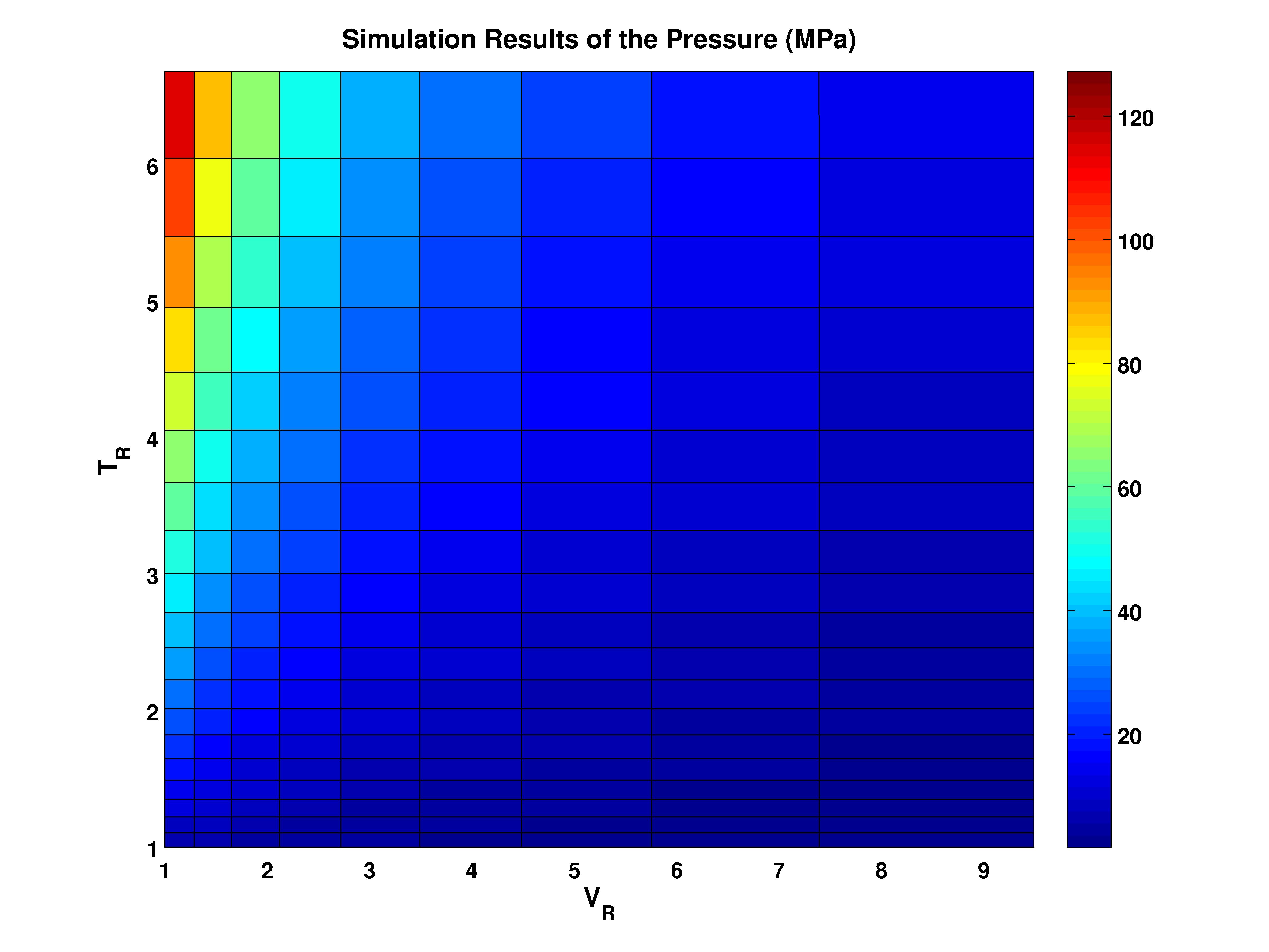
Figure 1: Simulation results of the pressure (MPa) of 1 mole of Argon, as a function of reduced temperature $T_{R}$ and reduced specific volume $V_{R}$.

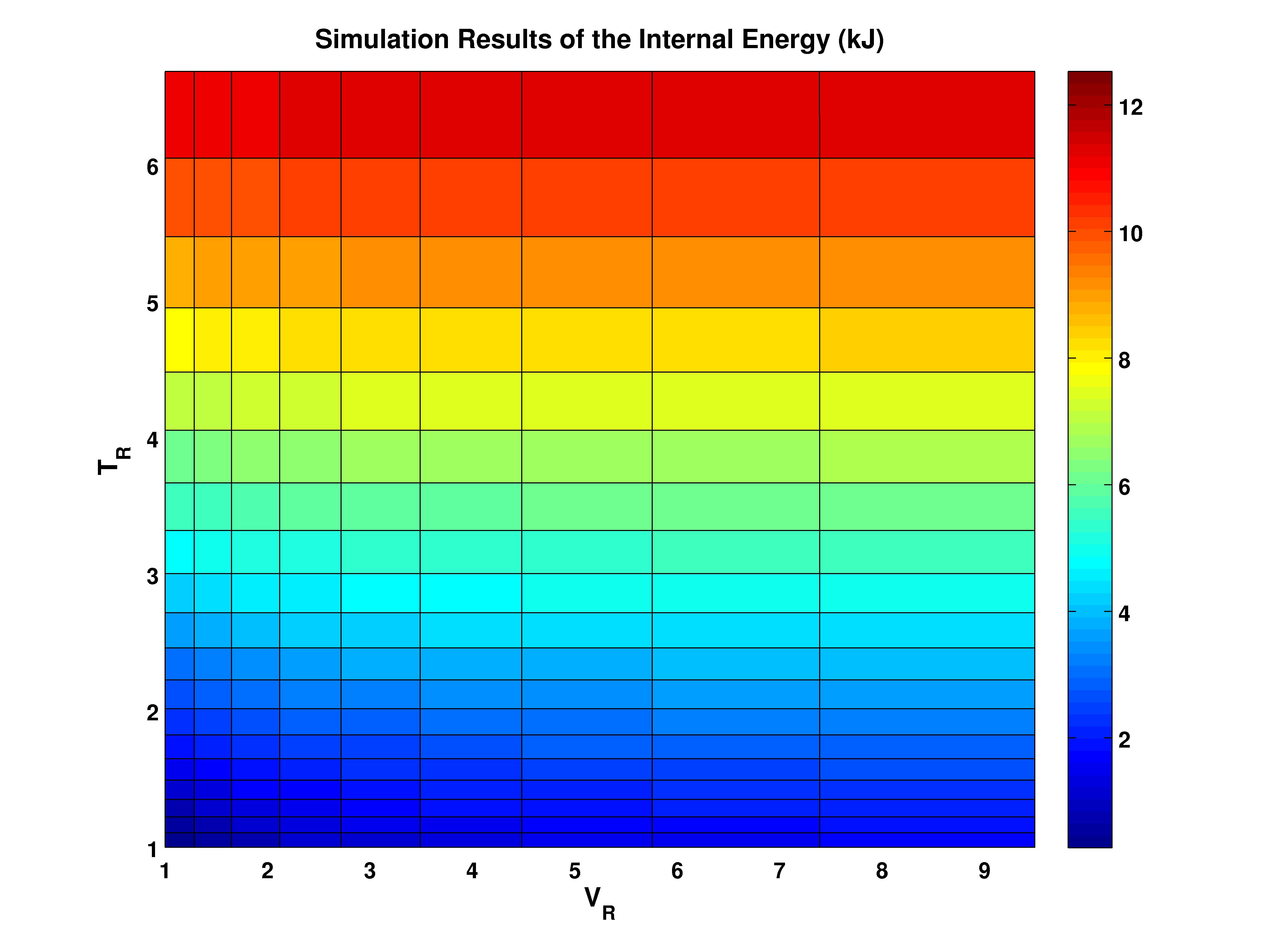
Figure 2: Simulation results of the internal energy U (kJ) of 1 mole of Argon, as a function of reduced temperature $T_{R}$ and reduced specific volume $V_{R}$.

At the colder and more dense parameters, the argon gas is far from ideal, where the pressure follows the equation of state defined in equation 7; a simulation will be considered to be ideal if its simulated pressure matches the ideal gas pressure with an error of less than 5%. In Figure 3, all of the ideal-gas parameters are colored in red, and the non-ideal parameters are colored blue; 76 out of the 200 parametric simulations was determined to represent ideal-gas argon. From these ideal gas parameters, the entropy was first determined with equation 22.

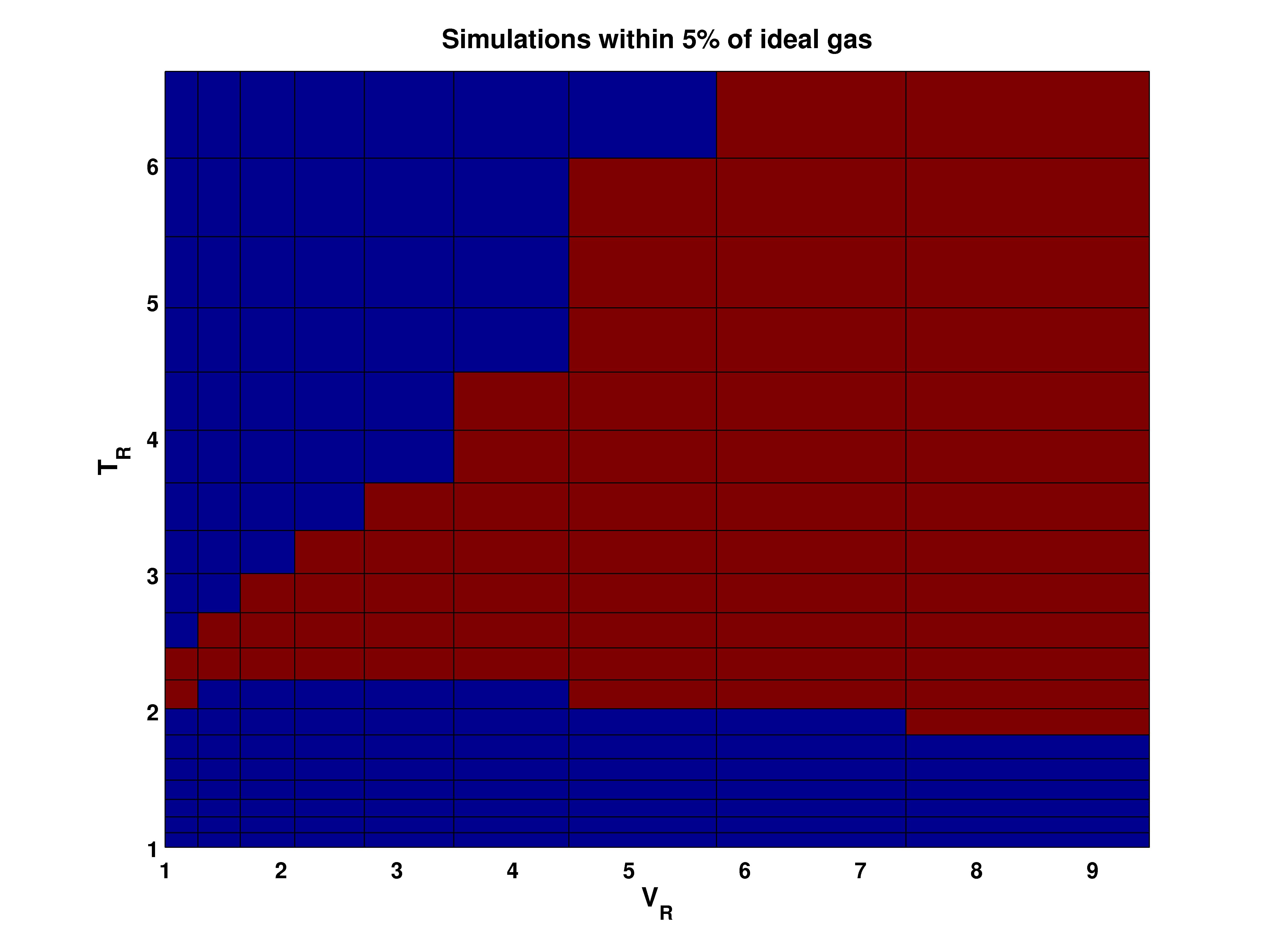
Figure 3: Location of parametric simulations that was determined to represent an ideal gas, where the pressure matched within 5% of the ideal gas pressure defined in equation 7.

Entropy is a measure of the disorder of a system, and the number of possible positions and velocities of a molecular system, and so it would make logical sense that as the entropy of a system of molecules increases, the standard deviations of the molecular positions and/or velocities would increase. The entropy of the ideal-gas argon was compared to the standard deviations of the argon molecule position $\sigma_{X}$ (m) and velocity $\sigma_{V}$ (m/s), and an empirical equation for the entropy as a function of the standard deviations was obtained (equation 47) with a correlation of R=0.9909 (Figure 4).

$$S_{empirical} = {\Phi_{1}}+{{\Phi_{2}}{\cdot}{\sqrt{{\sigma}_{V}}}}+{{\Phi_{3}}{\cdot}{\sqrt{{\sigma}_{X}}}},$$ (47)

$${{\sigma}_{X}}(m) = \sqrt{{{{{\sigma}_{X,x}}}^{2}}+{{\sigma}_{X,y}^{2}}+{{\sigma}_{X,z}^{2}}},$$

$${{\sigma}_{V}}(m/s) = \sqrt{{{\sigma}_{V,x}^{2}}+{{\sigma}_{V,y}^{2}}+{{\sigma}_{V,z}^{2}}},$$

$$\Phi_{1} = {106.239}{\quad}{\frac{J}{K}},$$

$$\Phi_{2} = 918.9098{\cdot}{10^{-4}}{\quad}{\frac{J}{K}}{\sqrt{\frac{s}{m}}},$$

$$\Phi_{3} = 0.13937{\cdot}{10^{-4}}{\quad}{\frac{J}{K}}{\sqrt{\frac{1}{m}}}.$$

The combined position and velocity standard deviation of all of the parameters, both ideal-gas parameters and real-gas parameters, are plotted in Figures 5 and 6, respectively. Taking these standard deviations, and using them in the empirical equation 47, the entropy S (J/K) of every parameter in this simulation is plotted in Figure 7.

Figure 4: Comparison of the entropy for the 76 parametric simulations (out of 200) that are considered to be an ideal gas defined with equation 7 (Figure 3); the value of $S_{analytical}$ (J/K) is defined with the analytical equation 22, and $S_{empirical}$ (J/K) is defined with the empirical equation 47.

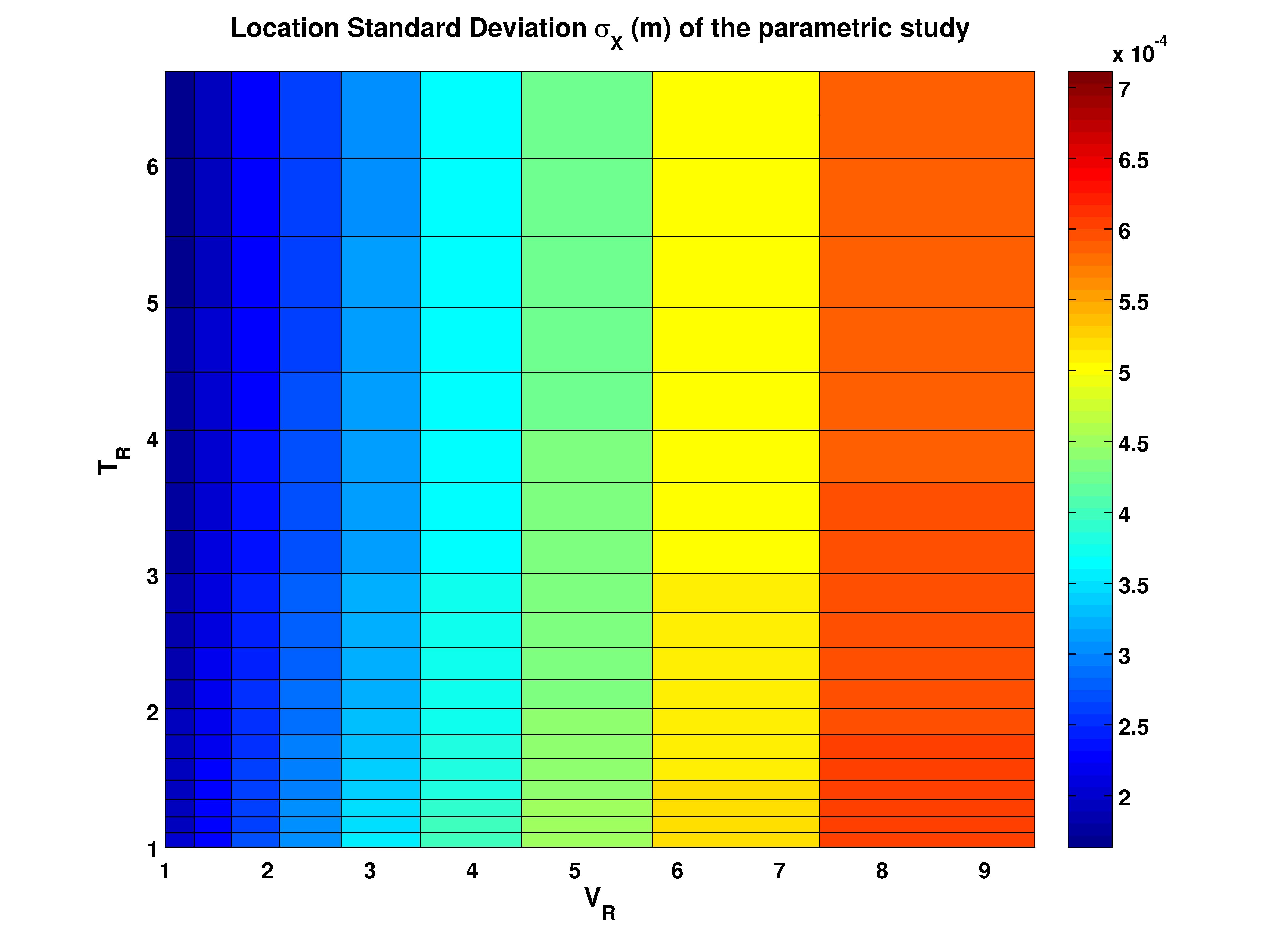
Figure 5: Location standard deviation $\sigma_{X}$ (m) of the parametric study.

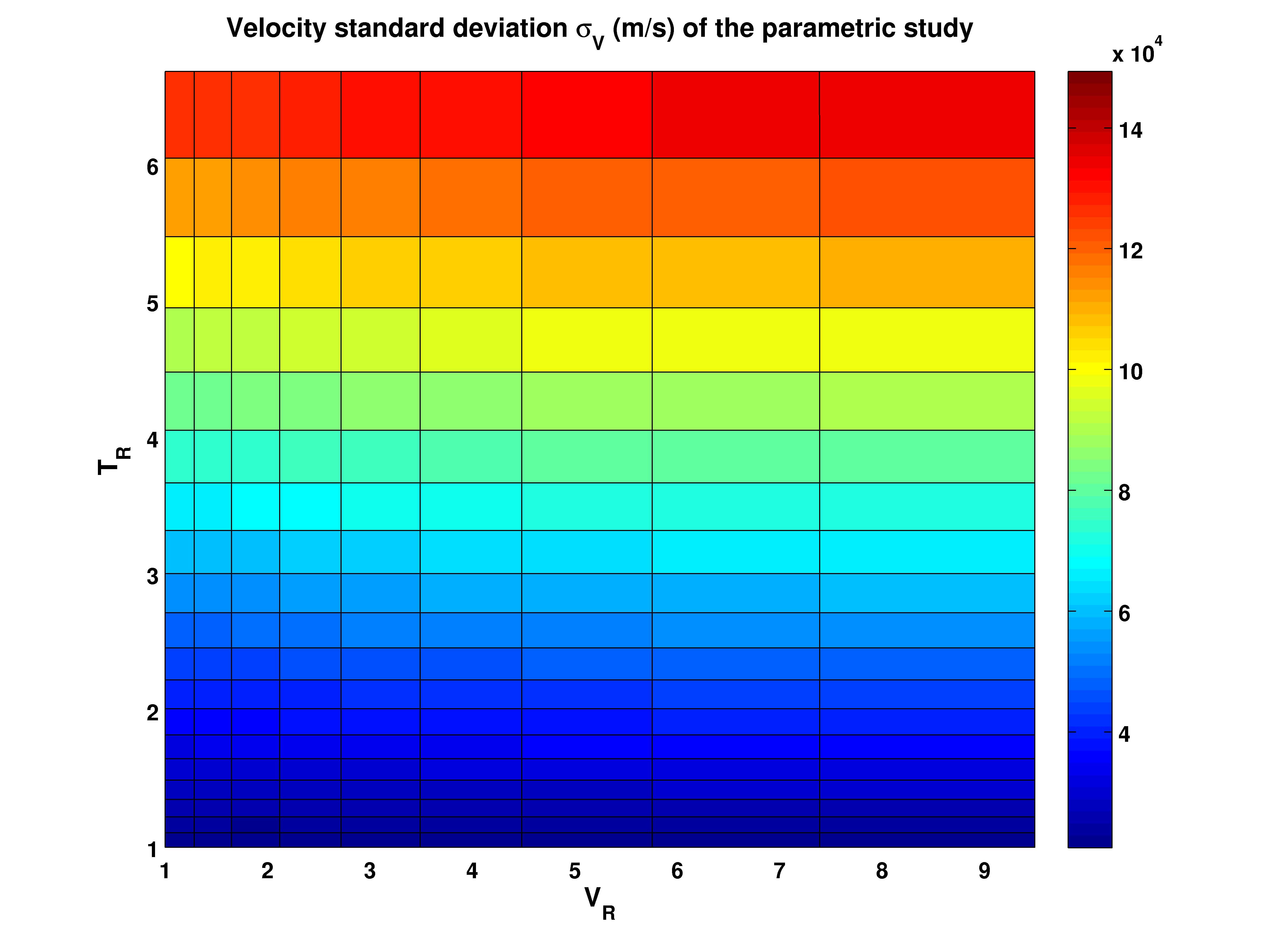
Figure 6: Velocity standard deviation $\sigma_{V}$ (m/s) of the parametric study.

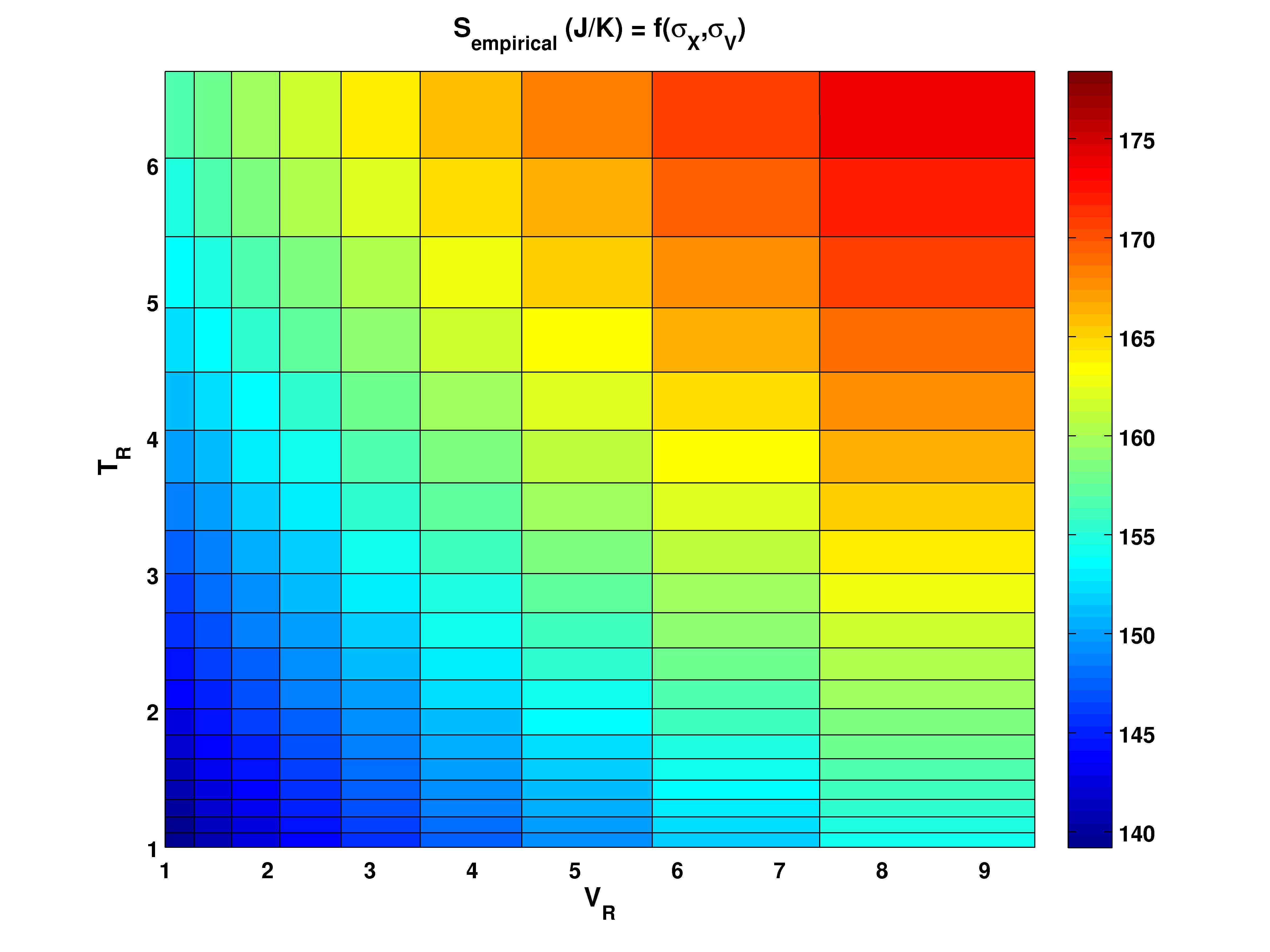
Figure 7: Entropy S (J/K) calculated with equation 47 as a function of both the (Figure 5) location standard deviation $\sigma_{X}$ (m) and the (Figure 6) velocity standard deviation $\sigma_{V}$ (m/s) of the parametric study.

The change in entropy for a mole of ideal-gas monatomic argon held at a constant volume would be calculated simply as

$${\delta}S=Q/T=1.5{\cdot}{R_{U}}{\cdot}{{\delta}T}/T,$$

however, this only applies to ideal gases. The rate of change in the entropy (Figure 7) was calculated, first for isochoric heating (constant volume), yielding 19$\cdot$10 or 190 different calculated rates of change, encompassing both ideal and real argon undergoing isochoric heating. It is desired to find an empirical equation for the change in entropy as a function of the position $\sigma_{X}$ (m) and velocity $\sigma_{V}$ (m/s) standard deviation, as well as the heat input Q (J). The heat input at a constant volume can be determined with the first law (equation 1), and thus

$$Q = {\delta}U,$$ (48)

and the change in the internal energy U can be determined from the data plotted in Figure 2. The empirical equation found (equation 49) calculates the change in entropy ${\delta}S_{{\delta}v=0}$ (J/K) of isochoric heating as a function of the heat input Q (J), the position standard deviation $\sigma_{X}$ (m), and the velocity standard deviation $\sigma_{V}$ (m/s),

$${\delta}S_{{\delta}v=0} = {{T_{1}}{\cdot}{Q}}+{{T_{2}}{\cdot}{{\sigma}_{V}}}+{{T_{3}}{\cdot}{{\sigma}_{X}}},$$ (49)

$$T_{1} = 7.7664{\cdot}{10^{-4}}{\quad}{\frac{1}{K}},$$

$$T_{2} = 17.6815{\cdot}{10^{-4}}{\quad}{\frac{J{\cdot}s}{K{\cdot}m}},$$

$$T_{3} = 9.1519{\quad}{\frac{J}{K{\cdot}m}}.$$

This equation 49 was found to match the change in entropy of the data in Figure 7 with a correlation R of 0.99025 (Figure 8).

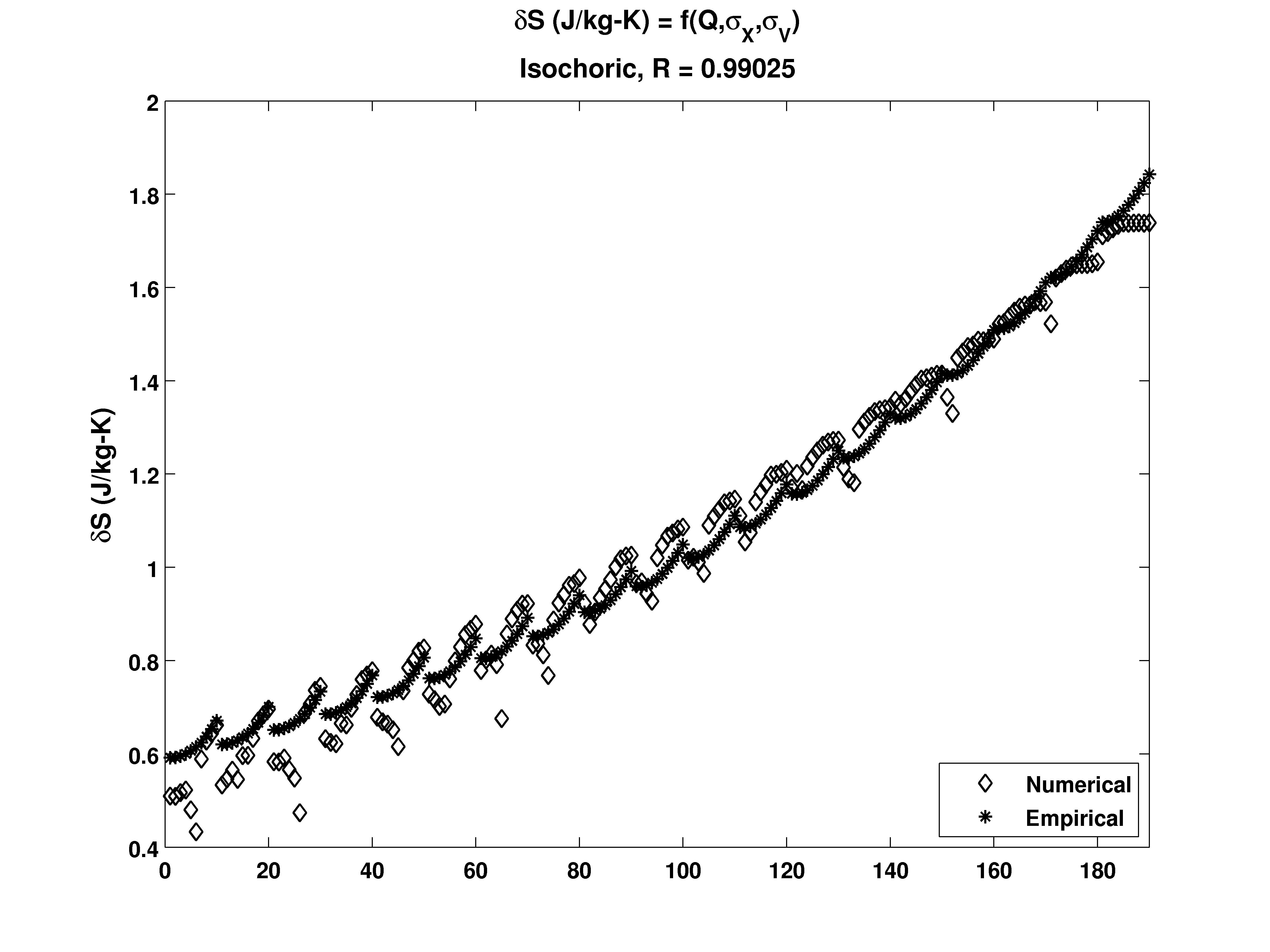
Figure 8: The rate of change in entropy ${\delta}S_{{\delta}v=0}$ (K) for isochoric heating, comparing both the entropy data in Figure 7, and using the empirical equation 49. The empirical equation was found to match the numerical data with a correlation R of 0.99025.

The rate of change in the entropy (Figure 7) was next calculated for isothermal expansion (constant temperature), yielding 20$\cdot$9 or 180 different calculated rates of change, encompassing both ideal and real argon undergoing isothermal expansion heating. The heat input during isothermal expansion can be determined with the first law (equation 1), and thus

$$Q={{\delta}U}+{P{\cdot}{{\delta}V}},$$ (50)

where the change in the internal energy ${\delta}U$ (J) can be determined from the data plotted in Figure 2, and the change in pressure P (Pa) and volume ${\delta}V$ (m³) can be determined with the numerically obtained pressures plotted in Figure 1. The empirical equation found (equation 51) calculates the change in entropy ${\delta}S_{{\delta}T=0}$ (J/K) of isothermal expansion heating as a function of the heat input Q (J), the position standard deviation $\sigma_{X}$ (m), and the velocity standard deviation $\sigma_{V}$ (m/s),

$${\delta}S_{{\delta}T=0} = {{V_{1}}{\cdot}{Q}{\cdot}{\frac{{\sigma}_{X}}{{\sigma}_{V}}}},$$ (51)

$$V_{1} = {311,594.4735}{\quad}{\frac{J}{K{\cdot}s}}.$$

This equation 51 was found to match the change in entropy of the data in Figure 7 with a correlation R of 0.99433 (Figure 9).

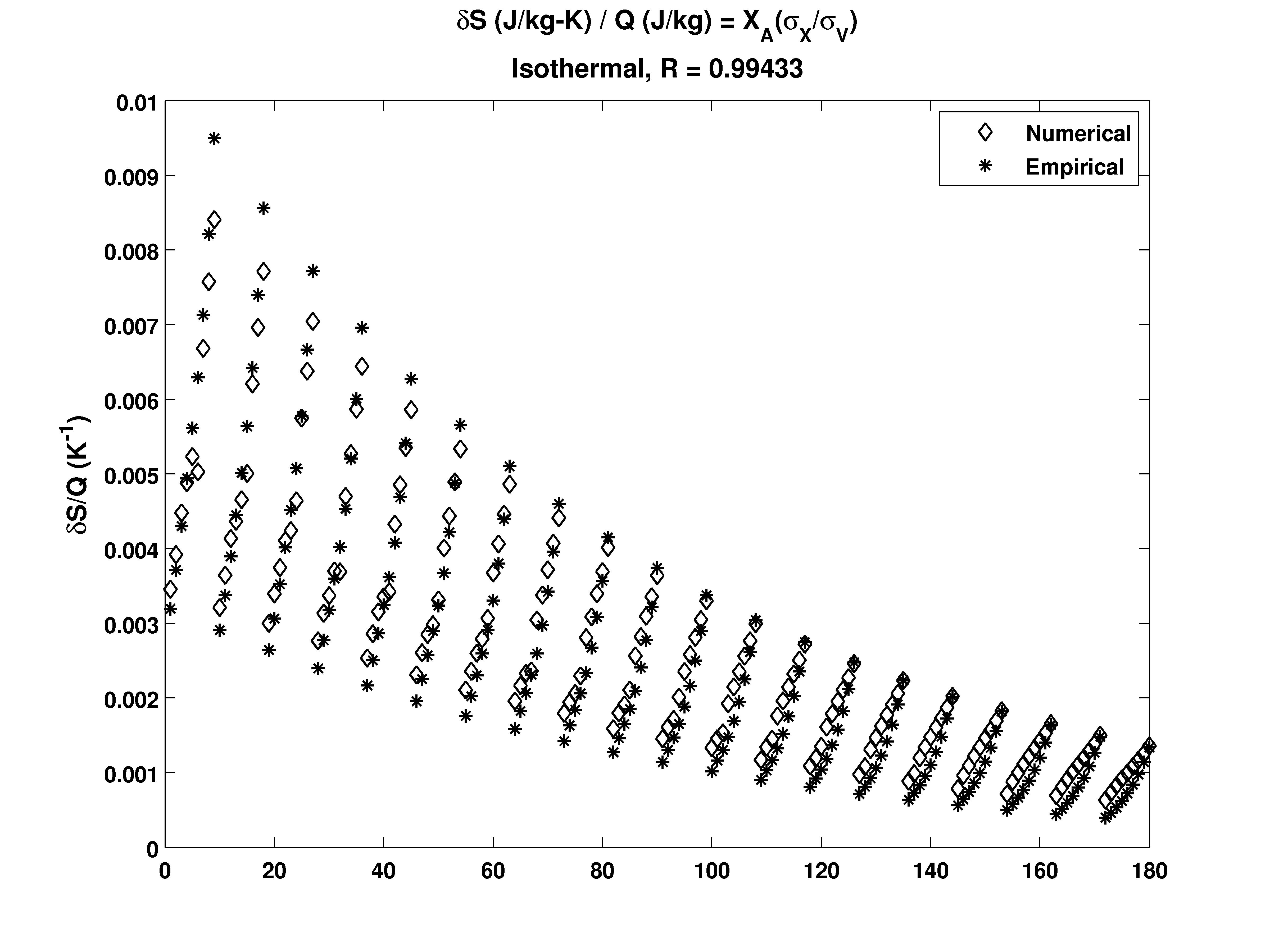
Figure 9: The rate of change in entropy ${\delta}S_{{\delta}T=0}$ (K) for isothermal expansion, comparing both the entropy data in Figure 7, and using the empirical equation 51. The empirical equation was found to match the numerical data with a correlation R of 0.99433.

VI The Supercritical Stirling Cycle Heat Engine

The supercritical Stirling cycle heat engine was analyzed in an earlier effort MarkoAIP , where a real fluid (argon) is compressed isothermally at a cold temperature (Stage 1-2), heated at a constant volume to a hot temperature (Stage 2-3), expanded isothermally at the hot temperature (Stage 3-4), and cooled at a constant volume back to the original cold temperature (Stage 4-1). The numerical results at the end of this parametric study can represent a supercritical Stirling cycle, where the coldest temperature data is used for the isothermal compression (Stage 1-2), the smallest volume data is used for the isochoric heating (Stage 2-3), the hottest temperature data is used for the isothermal expansion (Stage 3-4), and the largest volume is used for the isochoric cooling (Stage 4-1). The numerically obtained reduced pressure $P_{R}$ and reduced specific volume $V_{R}$ of this cycle is plotted in Figure 10. The change in internal energy ${\delta}U$ (J), work input and output $W={P{\cdot}{{\delta}V}}$ (J) obtained with equation 2, and heat input Q (J) determined with equations 48 and 51, are plotted in Figure 11.

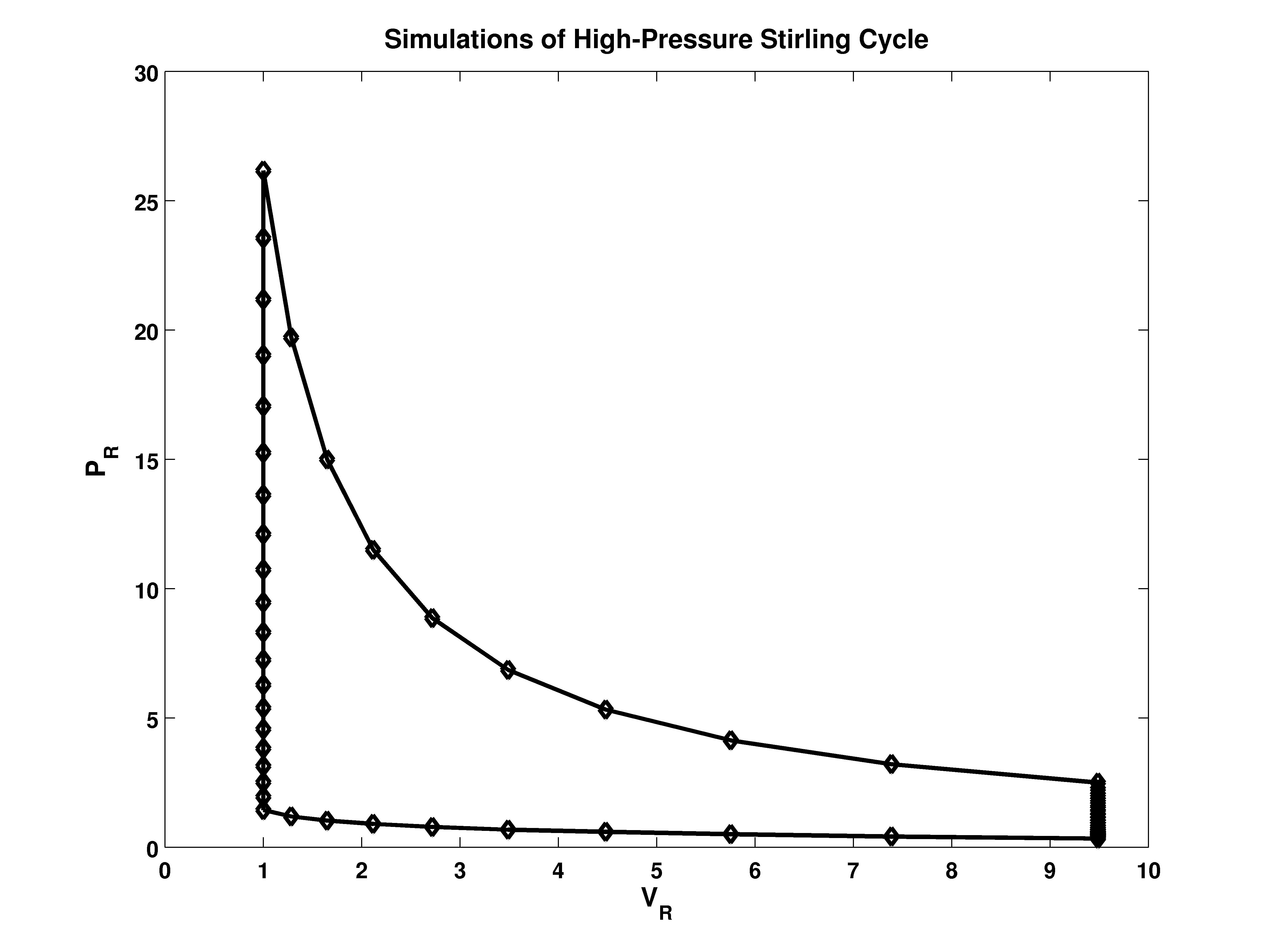
Figure 10: Reduced pressure $P_{R}$ and reduced specific volume $V_{R}$ for the supercritical Stirling cycle heat engine.

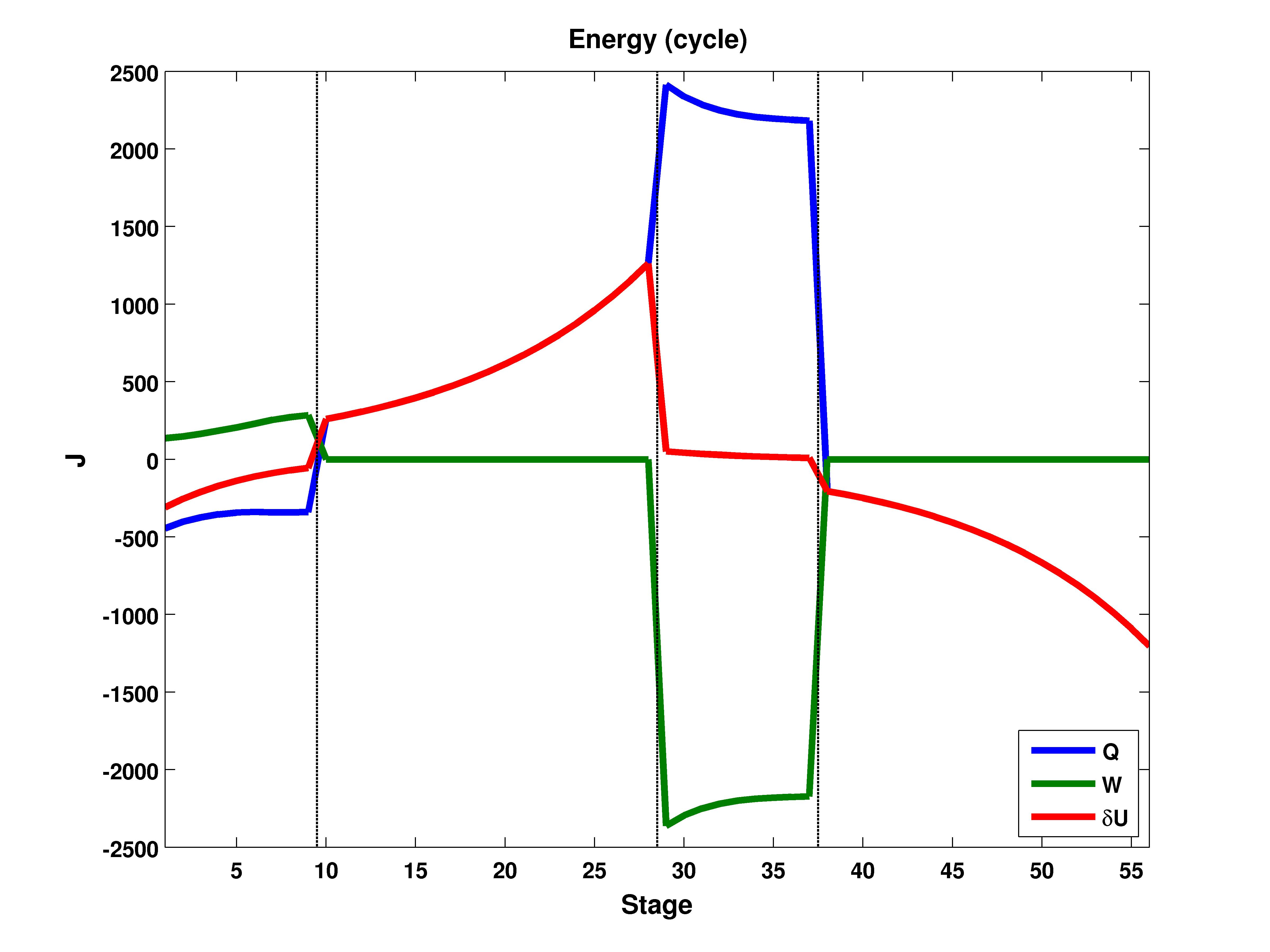
Figure 11: The change in internal energy ${\delta}U$ (J) obtained from Figure 2, the work input and output W (J) obtained with equation 2, and the heat input and output Q (J) obtained with equations 48 and 50; for the supercritical Stirling cycle heat engine defined in Figure 10.

Within Figure 12, the change in entropy determined with equation 47 (Figure 7) is plotted as ${\delta}S_{\sigma}$ (J/K), alongside the cumulative change in entropy ${\delta}S_{U}$ (J/K) plotted as a function of the heat input Q (J) over the temperature T (K), as defined in equation 4. Assuming the surrounding environment is an ideal gas, and heat transfer always occurs at the temperature of the argon (nil temperature differential), it is observed that ${\delta}S_{U}$ and ${\delta}S_{\sigma}$ do not match perfectly.

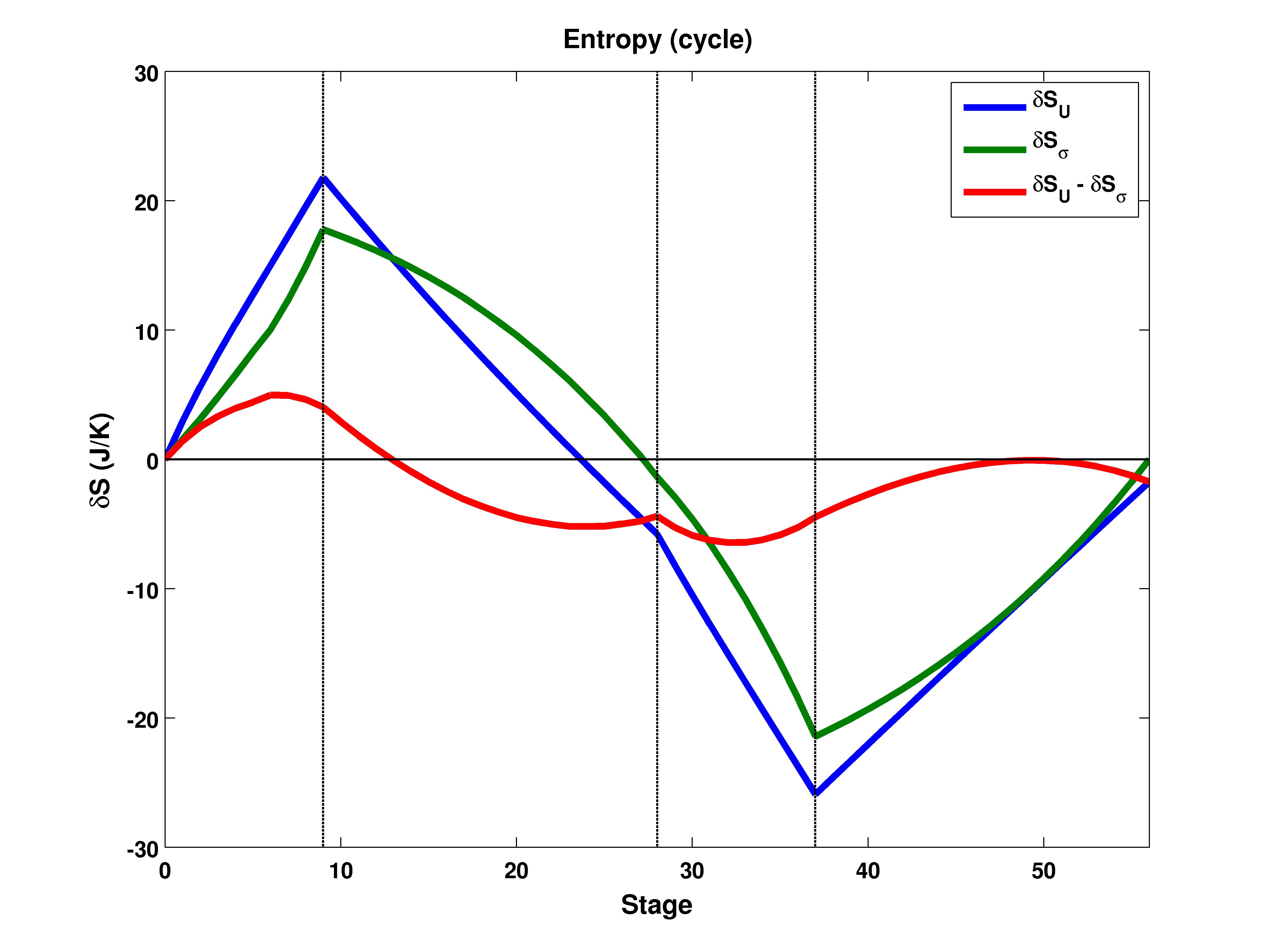
Figure 12: The cumulative change in entropy ${\delta}{S}$ (J/K) for the supercritical Stirling cycle heat engine defined in Figure 10; both ${\delta}S_{U}$ (J/K) defined with equation 4, and ${\delta}S_{\sigma}$ (J/K) defined with the numerical simulation results (Figure 7).

VII Conclusion

The change in entropy to the surrounding ${\delta}{S_{U}}$ assumes heat transfer occurs at a virtually identical temperature between the surrounding and the argon. As expected, it is clear looking at Figure 12 that while the entropy of the fluid increases, the entropy of the surrounding universe is decreasing (and vice versa); it is observed, however, that the magnitude in the change in entropy is consistently different despite the fact that identical heat transfer occurs at identical temperatures. The net change in entropy at the conclusion of this cycle $({\int}{\delta}{S_{U}}-{\int}{\delta}{S_{\sigma}})$ is -1.7463 J/K, suggesting a net reduction of entropy to the universe for each revolution of one mole of high-pressure argon throughout this cycle, due to the intermolecular attractive Van der Waal force MarkoAIP . In addition, the net entropy of the high-pressure argon working fluid ${\int}{\delta}{S_{\sigma}}$ is 0 J/K as this cycle is internally reversible.

One observation is that the total entropy of the real-fluid argon, when utilizing the empirical equation 47 and the numerically obtained standard deviations for the molecule position $\sigma_{X}$ (m) and velocity $\sigma_{V}$ (m/s), is consistently greater than for a mole of ideal gas argon of comparable temperature (equation 22). The intermolecular attractive forces add to the RMS velocities (typically 10% increase), and require the molecules to travel (on average) a longer spatial distance to move throughout the spherical container. In empirical equation 49, there is a clear positive correlation between the increase in entropy (for a given heat input) and the standard deviation of the molecules velocity and position for isochoric heating. The discrepancy in entropy makes it clear that the ideal-gas equation for entropy (equation 4), while absolutely appropriate for idea gases, does not apply to real non-ideal fluids if trying to determine the disorder and the number of states as defined by Boltzman’s equation 6. This study makes it clear that entropy is better defined by looking at the numerically obtained standard deviations of the positions $\sigma_{X}$ (m) and velocity $\sigma_{V}$ (m/s), and using the empirical equation 47 when dealing with real fluids subjected to the intermolecular attractive Van der Waal forces.

Fortran Code

      program MakeInput
      implicit none

      real Vr,Tr,Vr_Fct(200),Tr_Fct(200)
      real U,S_entropy,P_kinetic,P_PR
      double precision pi,Kb,Av
      real t1,t2,Rat(100),outputdat(22)
      integer fooint,ct,ctx,ii,jj,kk,ppnum
      character(len=17) filenameSV


      call CPU_Time(t1)

      pi=3.1415926535897932384626
      Kb=1.38064852e-23  ! Boltzman’s Constant
      Av=6.02214086e23   ! Avogadro’s Number


c ---- Run a parametric series, first four separate heating simulations,
c ---- then four stages of the high-pressure Stirling cycle



      ct=0
      do ii=1,20
        Tr=1.0*exp((ii-1)*0.10)
        do jj=1,10
          ct=ct+1
          Vr=1.0*exp((jj-1)*0.25)
          Tr_Fct(ct)=Tr
          Vr_Fct(ct)=Vr
        enddo
      enddo

      ctx=200
      open(unit=1000,file=’param_output_data_study_8sept2020.txt’)
      ppnum=0

      do ii=1,200
        ppnum=ppnum+1
        Tr=Tr_Fct(ii)
        Vr=Vr_Fct(ii)
        call ThermoCalc(Vr,Tr,ppnum,outputdat)
        call CPU_Time(t2)

        if (ppnum<10) then
          write(filenameSV,’("Save_00",I1,".txt")’)ppnum
        elseif (ppnum<100) then
          write(filenameSV,’("Save_0",I2,".txt")’)ppnum
        elseif (ppnum<1000) then
          write(filenameSV,’("Save_",I3,".txt")’)ppnum
        endif
        open(unit=ppnum,file=filenameSV)
        write(ppnum,*) ppnum,Vr,Tr,outputdat,’t (s) = ’,(t2-t1)
        close(ppnum)


        write(1000,*) ppnum,Vr,Tr,outputdat,’t (s) = ’,(t2-t1)
        print *,ppnum,’/’,ctx,’t (s) = ’,t2
      enddo


      close(1000)

      end program


c ------------------------------- Analysis Subroutine ----------------------------

      subroutine ThermoCalc(Vr,Tr,ppnum,outputdat)

      real, intent(in) :: Vr,Tr
      integer, intent(in) :: ppnum
      real, intent(out) :: outputdat(22)


      integer ctsplitrng,ctsplit,fooint

      real U,S_entropy,P_kinetic,P_PR
      real t1,t2
      double precision  MM,Pc,Tc,Vc,ecc,V,T,Rg,a,b,R,AreaS,minVr
      double precision  kappa,a_PR,xx(3),Vx(3),Vx0(3),RMS3(3)
      double precision  Coeff
      double precision  dP_VWD, F_VDW_m,phi,theta,Vel,dP_VDW,V_rms_0,V_avg_0
      double precision drX,Vel_travel(3),Vel_xx
      double precision VelF,Vrat(3),Xrat(3)
      double precision VXdot,dP_Pauli,P_IG,U_KE,U_PE
      double precision Read6(6),Avg6(6),StDev6(6),V_rms_calc,V_avg_calc

      character (len=200) output
      integer ii,ii0,jj,jj0,kk,ct,dir(3)
      integer dx0, Nx, Ny, Np, Total_CT
      double precision bp,aa
      double precision pi,Kb,Av,m_m,dt,Fx(3),fooV(2)
      double precision, allocatable :: phi_fct(:),theta_fct(:),rrX(:,:)
      double precision, allocatable :: VXrat(:),F_dat(:),VelFdat(:)
      double precision, allocatable :: Vel_travelDat(:),Vel_fct(:)
      double precision, allocatable :: Xstore(:,:),Vstore(:,:)
      double precision, allocatable :: Fx_Stored(:,:)
      double precision, allocatable :: foocrap(:),randnum(:)
      integer, allocatable :: Tct(:),Total_Ct_Fct(:)

      character(len=15) filenameSV

      call CPU_Time(t1)

c ------------------------------- Make Source -------------------------------


      pi=3.1415926535897932384626
      Kb=1.38064852e-23
      Av=6.02214086e23

      dx0=300   ! Estimated time steps per bounce
      Nx=91   ! Number of steps in each degree (square it in theta and phi)
      Ny=101   ! Number of steps at each degree increment, varying speed randomly
      ctsplit=500  ! Number of files to save all data (avoid limit of memory)


c --- Argon
      MM=.0399  ! Molar Mass (kg/mole)
      Pc=4.863e6  ! Critical Pressure (Pa)
      Tc=150.687  ! Critical Temperature (K)
      Vc=1./535    ! Critical Volume (m^3/kg)
      ecc=0       ! Eccentricity factor



c__________________________________________________

      Np=(Nx**2)*Ny  ! Total number of molecules bouncing in the spherical container

      if ((mod(Np,ctsplit))==0) then
        ctsplitrng=(Np/ctsplit)
      else
        ctsplitrng=(Np/ctsplit)+1
      endif
      print *,ctsplitrng

      ALLOCATE(rrX(Np,3))
      ALLOCATE(Tct(Np))
      ALLOCATE(VXrat(Np))
      ALLOCATE(F_dat(Np))
      ALLOCATE(VelFdat(Np))
      ALLOCATE(Vel_travelDat(Np))
      ALLOCATE(Vel_fct(Np))
      ALLOCATE(Xstore((dx0*10),3))
      ALLOCATE(Vstore((dx0*10),3))
      ALLOCATE(Fx_Stored((dx0*10),3))
      ALLOCATE(randnum(Ny))
      ALLOCATE(Total_Ct_Fct(ctsplit))

      ALLOCATE(foocrap(Np))

      V=Vr*Vc*MM  ! Actual volume (m^3)
      T=Tr*Tc     ! Actual temperature (K)

      m_m=MM/Av   ! Mass of Argon molecule
      Rg=Av*Kb/MM ! Gas Constant

c --- Peng-Robinson Equation of State coefficients
      a=0.45724*(Rg**2)*(Tc**2)/Pc
      b=0.07780*Rg*Tc/Pc

c --- Ensure the volume is not excessively small
      minVr=1./100
      if (Vr<((1+minVr)*b/Vc)) then
            V=((1+minVr)*b/Vc)*Vc*MM
      endif

c --- Coefficient for change in internal energy
      bp=(2.**(1./3))-1.
      aa=(1/(9*bp))*(Rg**2)*(Tc**2.5)/Pc


c --- R = Radius of Sphere; Rb = equivalent radius of sphere (Pauli Exclusion)

      R=(V*(3./(4*pi)))**(1./3)
      Rb=((V-(b*MM))*(3./(4*pi)))**(1./3)
      AreaS=4*pi*(R**2) ! Surface Area of sphere

      V_rms_0=sqrt(3*Kb*T/m_m) ! RMS velocity of molecule
      V_avg_0=V_rms_0*(sqrt(8/(3*pi))) ! Average velocity of molecule

c --- Determine pressure from Peng-Robinson Equation of State
      kappa=0.37464+(1.54226*ecc)-(0.26992*(ecc**2))
      a_PR=(1.+(kappa*(1-(sqrt(T/Tc)))))**2
      P_PR=((Rg*T)/((V/MM)-b))
      P_PR=P_PR-((a_PR*a)/((((V/MM)**2)+(2*b*(V/MM))-(b**2))))


      dt=(2*R/V_avg_0)/dx0 ! Time step (s)


c --- Set function of angles in X-Y-Z coordinates
      ct=0
      do jj=1,Nx
            phi=(pi/2)*((jj-1.)/(Nx-1.))
            do ii=1,Nx
                  ct=ct+1
                  theta=(pi)*((ii-1.)/(Nx-1.))
                  xx(1)=(sin(theta))*(cos(phi))
                  xx(2)=(sin(theta))*(sin(phi))
                  xx(3)=cos(theta)


                  do kk=1,Ny
                        rrX(((ct-1)*Ny)+kk,1)=xx(1)
                        rrX(((ct-1)*Ny)+kk,2)=xx(2)
                        rrX(((ct-1)*Ny)+kk,3)=xx(3)
                  enddo
            enddo
      enddo

c --- Call velocity spread function (if Ny>1)
      call make_rand_fct(Ny,randnum)

c --- Confirm ratio of V_rms_calc / V_avg_calc = (pi*4/3)^(1/3)
      V_rms_calc=0
      V_avg_calc=0
      do ii=1,Ny
        V_avg_calc=V_avg_calc+(randnum(ii)*V_avg_0/Ny)
        V_rms_calc=V_rms_calc+(((randnum(ii)*V_avg_0)**2)/Ny)
      enddo
      V_rms_calc=sqrt(V_rms_calc)


c --- Set velocity function
      do ii=1,(Nx**2)
        do jj=1,Ny
          ii0=((ii-1)*Ny)+jj
          if (Ny==1) then
            Vel_fct(ii0)=V_rms_0
          else
c            Vel_fct(ii0)=V_rms_0
            Vel_fct(ii0)=(randnum(jj))*V_avg_0
          endif
        enddo
      enddo


c ------------------------------- Make Source -------------------------------


      ii=0
      Total_CT=0
      Total_CT0=0

c --- Actually run the simulation, and saving X-Y-Z data of molecule until
c --- it reaches the opposing surface of the spherical container

      do ii0=1,ctsplit

        if ((ii+ctsplitrng)>Np) then
          fooint=Np-ii
        else
          fooint=ctsplitrng
        endif

        if (ii0<10) then
          write(filenameSV,’("SaveXV3_00",I1,".txt")’)ii0
        elseif (ii0<100) then
          write(filenameSV,’("SaveXV3_0",I2,".txt")’)ii0
        elseif (ii0<1000) then
          write(filenameSV,’("SaveXV3_",I3,".txt")’)ii0
        endif
        open(unit=ii0,file=filenameSV)
        do jj0=1,fooint
          ii=ii+1

          call Get_dP_VDW(Vel_fct(ii),Vr,dP_VDW)
          F_VDW_m=dP_VDW*AreaS/Av
          Vx0=(Vel_fct(ii))*(rrX(ii,:))
          Vx=Vx0
          xx=xx*0
          xx(1)=-R
          drX=(sqrt(sum(xx**2)))*(0.99)

          Xstore=Xstore*0
          Vstore=Vstore*0
          Fx_Stored=Fx_Stored*0
          ct=0
          do while ((abs(drX/R))<1.0)
            ct=ct+1
            xx=xx+(Vx*dt)
            drX=(sqrt(sum(xx**2)))

            do jj=1,3
              if (xx(jj)==0) then
                dir(jj)=0
              else
                dir(jj)=-(xx(jj)/(abs(xx(jj))))
            endif
          enddo
          Fx=(abs(F_VDW_m*((xx/R)**3)))*dir
          do jj=1,3
            Vx(jj)=Vx(jj)+(Fx(jj)*dt/m_m)
          enddo
          write(ii0,*) xx(:),Vx(:)

          do jj=1,3
            Xstore(ct,jj)=xx(jj)
            Vstore(ct,jj)=Vx(jj)
            Fx_Stored(ct,jj)=Fx(jj)
          enddo
          if (ct>(dx0*10)) then
            drX=10*R
            print *,’PROBLEM!!!’,ct,dx0
          endif

          enddo

          Tct(ii)=ct
          Total_CT0=Total_CT0+ct
          Total_CT=Total_CT+ct
          Vel_travel=Vel_travel*0
          do jj=1,3
            fooreal1=0
            do kk=1,ct
              fooreal1=fooreal1+(Vstore(kk,jj)/ct)
            enddo
            Vel_travel(jj)=fooreal1
          enddo
          do jj=1,3
            Vel_travelDat(ii)=Vel_travelDat(ii)+(Vel_travel(jj)**2)
          enddo
          Vel_travelDat(ii)=sqrt(Vel_travelDat(ii))


          VelF=0
          do jj=1,3
            VelF=VelF+(Vstore(ct,jj)**2)
          enddo
          VelF=sqrt(VelF)
          VelFdat(ii)=VelF

          Vrat=Vstore(ct,:)/VelF
          Xrat=xx/R

          VXdot=0
          do jj=1,3
            VXdot=VXdot+(Xrat(jj)*Vrat(jj))
          enddo
          VXrat(ii)=VXdot

c ------- Calculate the force, to numerically determine the pressure
          F_dat(ii)=((2*m_m*VXdot)*VelF/(ct*dt))-F_VDW_m

        enddo
        close(ii0)
        Total_Ct_Fct(ii0)=Total_Ct0
        Total_Ct0=0
      enddo

c --- Calculate the average and RMS position and velocity of the molecules

      Avg6=Avg6*0.
      RMS3=RMS3*0.
      StDev6=StDev6*0.

      do jj=1,ctsplit

        if (jj<10) then
          write(filenameSV,’("SaveXV3_00",I1,".txt")’)jj
        elseif (jj<100) then
          write(filenameSV,’("SaveXV3_0",I2,".txt")’)jj
        elseif (jj<1000) then
          write(filenameSV,’("SaveXV3_",I3,".txt")’)jj
        endif
        open(unit=jj,file=filenameSV)

        do ii=1,(Total_Ct_Fct(jj))
          read(jj,*) Read6(:)
          Avg6=Avg6+Read6
          RMS3=RMS3+(Read6(4:6)**2.)
        enddo
        close(jj)
      enddo
      Avg6=Avg6/Total_CT
      RMS3=sqrt(RMS3/Total_CT)

c --- Calculate the standard deviation position and velocity of the molecules

      do jj=1,ctsplit

        if (jj<10) then
          write(filenameSV,’("SaveXV3_00",I1,".txt")’)jj
        elseif (jj<100) then
          write(filenameSV,’("SaveXV3_0",I2,".txt")’)jj
        elseif (jj<1000) then
          write(filenameSV,’("SaveXV3_",I3,".txt")’)jj
        endif
        open(unit=jj,file=filenameSV)

        do ii=1,(Total_Ct_Fct(jj))
          read(jj,*) Read6(:)
          StDev6=StDev6+((Read6-Avg6)**2)
        enddo
        close(jj)
      enddo
      StDev6=StDev6/Total_CT






c --- Output results of this specific trial

      P_kinetic=0
      U_KE=0
      S_entropy=0
      do ii=1,Np
            P_kinetic=P_kinetic+(F_dat(ii))
            U_KE=U_KE+(VelFdat(ii)**2)
            S_entropy=S_entropy+(Vel_travelDat(ii))
      enddo

      P_kinetic=((P_kinetic/Np)*(Av/AreaS))*(R/Rb)
      P_IG=Av*Kb*T/V

      U_KE=((U_KE/Np))*(0.5*Av*m_m)
      U_PE=-dP_VDW*V
      U=U_KE+U_PE
      S_entropy=((3*log(S_entropy/Np))+(log(V-(b*MM))))*Av*Kb

      outputdat(1)=U
      outputdat(2)=S_entropy
      outputdat(3)=P_kinetic
      outputdat(4)=P_PR
      outputdat(5:10)=Avg6
      outputdat(11:16)=StDev6
      outputdat(17:19)=RMS3
      outputdat(20)=Total_CT
      outputdat(21)=V_rms_calc
      outputdat(22)=V_avg_calc

      end subroutine

c ==========================================================


c ==========================================================

c --- Subroutine to calculate intermolecular attractive force component
c --- Equation developed to match Peng-Robinson equation of state

      subroutine Get_dP_VDW(Vel,Vr,dP_VDW)

      real, intent(in) :: Vr
      double precision, intent(in) :: Vel
      double precision, intent(out) :: dP_VDW
      double precision pi,Kb,Av,m_m,T_eff,Tr,Pc
      double precision MM,Tc,Vc,V,R,Coeff,Rb,bp,aa
      integer ii

      pi=3.1415926535897932384626
      Kb=1.38064852e-23
      Av=6.02214086e23

c     Argon
      MM=.0399  ! Molar Mass (kg/mole)
      Pc=4.863e6  ! Critical Pressure (Pa)
      Tc=150.687  ! Critical Temperature (K)
      Vc=1./535    ! Critical Volume (m^3/kg)
c      ecc=0       ! Eccentricity factor

      V=Vr*Vc*MM

      m_m=MM/Av
      Rg=Av*Kb/MM

      bp=(2.**(1./3))-1.
      aa=(1/(9*bp))*(Rg**2)*(Tc**2.5)/Pc

      T_eff=(Vel**2)*m_m/(3*Kb)
      Tr=T_eff/Tc


      if (Tr<1.) then
        Coeff=(2.3246+(-0.8441/(sqrt(Vr)))+(-0.8670))*Tr
      else
        Coeff=2.3246+(-0.8441/(sqrt(Vr)))+(-0.8670*sqrt(Tr))
      endif
      if (Coeff>1) then
        Coeff=0
      endif

      dP_VDW=(aa/(sqrt(T_eff)))/((V/MM)**2)
      dP_VDW=dP_VDW*Coeff


      end subroutine

c ==========================================================

c ==========================================================


c --- Subroutine to distribute velocities of molecules
c --- Ensures proper ratio of average and RMS velocity

      subroutine make_rand_fct(NN,randdat)

      integer, intent(in) :: NN
      double precision, intent(out) :: randdat(NN)

      double precision , allocatable :: NormFct(:),Xfct(:)
      double precision , allocatable :: NormFct0(:)
      double precision ctX,x,MinX,stdev0,dx,foo
      integer ii

c      ALLOCATE(randdat(NN))
      ALLOCATE(Xfct(NN))
      ALLOCATE(NormFct0(NN))
      ALLOCATE(NormFct(NN))

      MinX=0.200
      stdev0=0.71

      dx=((1.-MinX)*2.)/(NN-1)

      ctX=0.0
      do ii=1,NN
        x=MinX+((ii-1)*dx)
        Xfct(ii)=x
        NormFct(ii)=(exp(-0.5*(((x-1)/stdev0)**2)))
        ctX=ctX+(1./(exp(-0.5*(((x-1)/stdev0)**2))))
      enddo

      randdat(1)=MinX
      do ii=2,NN
        foo=(((1.-MinX)*2.)*(1./NormFct(ii))/ctX)
        randdat(ii)=randdat(ii-1)+foo
      enddo



      end subroutine

c ==========================================================

c ==========================================================

References

- [1] Sadi Carnot, E. Clapeyron, Rudolph Clausius, and E. Mendoza. Reflections on the Motive Power of Fire and other Papers on the Second Law of Thermodynamics. Dover Publications Inc, Mineola, NY, 1960.
- [2] Enrico Fermi. Thermodynamics. Dover Publications Inc, New York, NY, 1936.
- [3] Yunus A. Cengel and Michael A. Boles. Thermodynamics, An Engineering Approach Sixth Edition. McGraw Hill Higher Education, Columbus OH, 2008.
- [4] Daniel V. Schroeder. An Introduction to Thermal Physics. Addison Wesley Longman, Boston MA, 2000.
- [5] Terrell L. Hill. An Introduction to Statistical Thermodynamics. Dover Publications, 1960, 1960.
- [6] R. K. Pathria. Statistical Mechanics, 2nd Edition. Butterworth-Heinemann, 30 Corporate Drive, Suite 400, Burlington, MA 01803 USA, 1972.
- [7] Rongjia Yang. Is gravity entropic force. MDPI Entropy, 16:4483–4488, 2014. http://doi.org/10.3390/e16084483.
- [8] Takashi Torii. Violation of the third law of black hole thermodynamics in higher curvature gravity. MDPI Entropy, 14:2291–2301, 2012. http://doi.org/10.3390/e14112291.
- [9] Oyvind Gron. Entropy and gravity. MDPI Entropy, 14:2456–2477, 2012. http://doi.org/10.3390/e14122456.
- [10] Jeroen Schoenmaker. Historical and physical account on entropy and perspectives on the second law of thermodynamics for astrophysical and cosmological systems. MDPI Entropy, 16:4430–4442, 2014. http://doi.org/10.3390/e16084420.
- [11] Alessandro Pesci. Entropy bounds and field equations. MDPI Entropy, 17:5799–5810, 2015. http://doi.org/10.3390/e17085799.
- [12] Er Shi, Xiaoqin Sun, Yecong He, and Changwei Jiang. Effect of a magnetic quadrupole field on entropy generation in thermomagnetic convection of paramagnetic fluid with and without a gravitational field. MDPI Entropy, 19:96, 2017. http://doi.org/10.3390/e19030096.
- [13] J. Rossnagel, F. Schmidt-Kaler O. Abah, K. Singer, , and E. Lutz. Nanoscale heat engine beyond the carnot limit. Physical Review Letters, 112:030602, 22 January 2014. http://doi.org/10.1103/PhysRevLett.112.030602.
- [14] Jan Klaers, Stefan Faelt, Atac Imamoglu, and Emre Togan. Squeezed thermal reservoirs as a resource for a nanomechanical engine beyond the carnot limit. Physical Review X, 7:031044, 13 September 2017. http://doi.org/10.1103/PhysRevX.7.031044.
- [15] Nelly Huei Ying Ng, Mischa Prebin Woods, and Stephanie Wehner. Surpassing the carnot efficiency by extracting imperfect work. New Journal of Physics, 19:113005, 7 November 2017. http://doi.org/10.1088/1367-2630/aa8ced.
- [16] Matthew Marko. The saturated and supercritical stirling cycle thermodynamic heat engine cycle. AIP Advances, 8(8):085309, 2018. http://doi.org/10.1063/1.5043523.
- [17] M. Born and H.S. Green. A general kinetic theory of liquids, the molecular distribution functions. Proceedings of the Royal Society of London Series A Mathematical and Physical Sciences, 188, 1946. http://doi.org/10.1098/rspa.1946.0093.
- [18] Otto. Redlich and J. N. S. Kwong. On the thermodynamics of solutions. v. an equation of state. fugacities of gaseous solutions. Chemical Reviews, 44(a):233–244, 1949. http://doi.org/10.1021/cr60137a013.
- [19] Ding-Yu Peng and Donald B. Robinson. A new two-constant equation of state. Industrial and Engineering Chemistry Fundamentals, 75(1):59–64, 1976. http://doi.org/10.1021/i160057a011.
- [20] Kenneth S. Pitzer. Origin of the acentric factor. American Chemical Society Symposium Series, Phase Equilibria and Fluid Properties in the Chemical Industry, 60.
- [21] W.H. Keesom. The second viral coefficient for rigid spherical molecules, whose mutual attraction is equivalent to that of a quadruplet placed at their centre. Royal Netherlands Academy of Arts and Sciences Proceedings, 18 I:636–646, 1915.
- [22] Fabio L. Leite, Carolina C. Bueno, Alessandra L. Da Róz, Ervino C. Ziemath, and Osvaldo N. Oliveira Jr. Theoretical models for surface forces and adhesion and their measurement using atomic force microscopy. MDPI Molecular Sciences, 13:12773–12856, 2012. http://doi.org/10.3390/ijms131012773.
- [23] The General Theory of Molecular Forces. F. london. Transactions of the Faraday Society, 33:8–26, 1937. http://doi.org/10.1039/TF937330008B.
- [24] Roger H. French. Origins and applications of london dispersion forces and hamaker constants in ceramics. Journal of the American Ceramic Society, 83:2117–2146, 2000. http://doi.org/10.1111/j.1151-2916.2000.tb01527.x.
- [25] A. D. McLachlan. Retarded dispersion forces in dielectrics at finite temperatures. Proceedings of the Royal Society of London. Series A, Mathematical and Physical Sciences, 274:80–90, 1963. http://doi.org/10.1098/rspa.1963.0115.
- [26] M.H. Hawton, V.V. Paranjape, and J. Mahanty. Temperature dependence of dispersion interaction, application to van der waals forces and the polaron. Physical Review B, 26:1682–1688, 1982. http://doi.org/10.1103/PhysRevB.26.1682.
- [27] P.J. Linstrom and Eds W.G. Mallard. NIST Chemistry WebBook, NIST Standard Reference Database Number 69. National Institute of Standards and Technology, Gaithersburg MD, 20899, April 29 2018. http://doi.org/10.18434/T4D303.
- [28] Reiner Tillner-Roth and Hans Dieter Baehr. An international standard formulation for the thermodynamic properties of 1,1,1,2-tetrafluoroethane (hfc-134a) for temperatures from 170 k to 455 k and pressures up to 70 mpa. Journal of Physical and Chemical Reference Data, 23(5):657–729, 1994. http://doi.org/10.1063/1.555958.
- [29] Roland Span, Eric W. Lemmon, Richard T Jacobsen, Wolfgang Wagner, and Akimichi Yokozeki. A reference equation of state for the thermodynamic properties of nitrogen for temperatures from 63.151 to 1000 k and pressures to 2200 mpa. Journal of Physical and Chemical Reference Data, 29(6):1361–1433, 2000. http://doi.org/10.1063/1.1349047.
- [30] W. Wagner and A. Prub. The iapws formulation 1995 for the thermodynamic properties of ordinary water substance for general and scientific use. Journal of Physical and Chemical Reference Data, 31(2):387–535, 2002. http://doi.org/10.1063/1.1461829.
- [31] U. Setzmann and W. Wagner. A new equation of state and tables of thermodynamic properties for methane covering the range from the melting line to 625 k at pressures up to 100 mpa. Journal of Physical and Chemical Reference Data, 20(6):1061–1155, 1991. http://doi.org/10.1063/1.555898.
- [32] Daniel G. Friend, Hepburn Ingham, and James F. Fly. Thermophysical properties of ethane. Journal of Physical and Chemical Reference Data, 20(2):275–347, 1991. http://doi.org/10.1063/1.555881.
- [33] H. Miyamoto and K. Watanabe. A thermodynamic property model for fluid-phase propane. International Journal of Thermophysics, 21(5):1045–1072, 2000. http://doi.org/10.1023/A:1026441903474.
- [34] H. Miyamoto and K. Watanabe. Thermodynamic property model for fluid-phase n-butane. International Journal of Thermophysics, 22(2):459–475, 2001. http://doi.org/10.1023/A:1010722814682.
- [35] H. Miyamoto and K. Watanabe. A thermodynamic property model for fluid-phase isobutane. International Journal of Thermophysics, 23(2):477–499, 2002. http://doi.org/10.1023/A:1015161519954.
- [36] Richard B. Stewart and Richard T. Jacobsen. Thermodynamic properties of argon from the triple point to 1200 k with pressures to 1000 mpa. Journal of Physical Chemistry Reference Data, 18(1):639–798, 1989. http://doi.org/10.1063/1.555829.
- [37] Ch. Tegeler, R. Span, and W. Wagner. A new equation of state for argon covering the fluid region for temperatures from the melting line to 700 k at pressures up to 1000 mpa. Journal of Physical Chemistry Reference Data, 28(3):779–850, 1999. http://doi.org/10.1063/1.556037.
- [38] M. A. Anisimov, A. T. Berestov, L. S. Veksler, B. A. Kovalchuk, and V. A. Smirnov. Scaling theory and the equation of state of argon in a wide region around the critical point. Soviet Physics JETP, 39(2):359–365, 1974.
- [39] Kwan Y Kim. Calorimetric studies on argon and hexafluoro ethane and a generalized correlation of maxima in isobaric heat capacity. PhD Thesis, Department of Chemical Engineering, University of Michigan, 1974.
- [40] William D. McCain Jr and Waldemar T. Ziegler. The critical temperature, critical pressure, and vapor pressure of argon. Journal of Chemical and Engineering Data, 12(2):199–202, 1967. http://doi.org/10.1021/je60033a012.
- [41] O. Sifner and J. Klomfar. Thermodynamic properties of xenon from the triple point to 800 k with pressures up to 350 mpa. Journal of Physical Chemistry Reference Data, 23(1):63–152, 1994. http://doi.org/10.1063/1.555956.
- [42] James A. Beattie, Roland J. Barriault, and James S. Brierley. The compressibility of gaseous xenon. ii. the virial coefficients and potential parameters of xenon. Journal of Chemical Physics, 19:1222, 1951. http://doi.org/10.1063/1.1748000.
- [43] H. H. Chen, C. C. Lim, and Ronald A. Aziz. The enthalpy of vaporization and internal energy of liquid argon, krypton, and xenon determined from vapor pressures. Journal of Chemical Thermodynamics, 7:191–199, 1975. http://doi.org/10.1016/0021-9614(75)90268-2.
- [44] Richard T. Jacobsen and Richard B. Stewart. Thermodynamic properties of nitrogen including liquid and vapor phases from 63k to 2000k with pressures to 10,000 bar. Journal of Physical Chemistry Reference Data, 2(4):757–922, 1973. http://doi.org/10.1063/1.3253132.
- [45] Lester Haar and John S. Gallagher. Thermodynamic properties of ammonia. Journal of Physical Chemistry Reference Data, 7(3):635–792, 1978. http://doi.org/10.1063/1.555579.
- [46] Nathan S. Osborne, Harold F. Stimson, and Defoe C. Ginnings. Measurements of heat capacity and heat of vaporization of water in the range 0 to 100 C. Part of Journal of Research of the National Bureau of Standards, 23:197–260, 1939.
- [47] N. S. Osborne, H. F . Stimson, and D. C. Ginnings. Calorimetric determination of the thermodynamic properties of saturated water in both the liquid and gaseous states from 100 to 374 C. J. Research NBS, 18(389):983, 1937.
- [48] H. Sato, K. Watanabe, J.M.H Levelt Sengers, J.S. Gallagher, P.G. Hill, J. Straub, and W. Wagner. Sixteen thousand evaluated experimental thermodynamic property data for water and steam. Journal of Physical Chemistry Reference Data, 20(5):1023–1044, 1991. http://doi.org/10.1063/1.555894.
- [49] Leighton B. Smith and Frederick G. Keyes. The volumes of unit mass of liquid water and their correlation as a function of pressure and temperature. Procedures of American Academy of Arts and Sciences, 69:285, 1934. http://doi.org/10.2307/20023049.
- [50] Nathan S. Osborne, Harold F. Stimson, and Defoe C. Ginnings. Thermal properties of saturated water and steam. Journal of Research of the National Bureau of Standards, 23:261–270, 1939.
- [51] D. M. Murphy and T. Koop. Review of the vapor pressures of ice and supercooled water for atmospheric applications. Q. J. R. Meteorological Society, 131:1539–1565, 2005. http://doi.org/10.1256/qj.04.94.
- [52] B. A. Younglove and J. F. Ely. Thermophysical properties of fluids, methane, ethane, propane, isobutane, and normal butane. Journal of Physical Chemistry Reference Data, 16(4):577–798, 1987. http://doi.org/10.1063/1.555785.
- [53] Manson Benedict, George B. Webb, and Louis C. Rubin. An empirical equation for thermodynamic properties of light hydrocarbons and their mixtures i. methane, ethane, propane and nbutane. AIP Journal of Chemical Physics, 8:334, 1940. http://doi.org/10.1063/1.1750658.
- [54] John Edward Lennard-Jones. On the determination of molecular fields. Proceedings of the Royal Society A, 106(738):463–477, 1924. http://doi.org/10.1098/rspa.1924.0082.