TWO RESULTS ON LAYERED PATHWIDTH AND LINEAR LAYOUTS

Abstract

Layered pathwidth is a new graph parameter studied by Bannister et al. (2015). In this paper we present two new results relating layered pathwidth to two types of linear layouts. Our first result shows that, for any graph $G$, the stack number of $G$ is at most four times the layered pathwidth of $G$. Our second result shows that any graph $G$ with track number at most three has layered pathwidth at most four. The first result complements a result of Dujmović and Frati (2018) relating layered treewidth and stack number. The second result solves an open problem posed by Bannister et al. (2015).

1 Introduction

The treewidth and pathwidth of a graph are important tools in structural and algorithmic graph theory. Layered treewidth and layered $H$-partitions are recently developed tools that generalize treewidth. These tools played a critical role in recent breakthroughs on a number of longstanding problems on planar graphs and their generalizations, including the queue number of planar graphs [13], the nonrepetitive chromatic number of planar graphs [12], centered colourings of planar graphs [8], and adjacency labelling schemes for planar graphs [7, 11].

Motivated by the versatility and utility of layered treewidth, Bannister et al. [2, 3] introduced layered pathwidth, which generalizes pathwidth in the same way that layered treewidth generalizes treewidth. The goal of this article is to fill the gaps in our knowledge about the relationship between layered pathwidth and the following well studied linear graph layouts: queue-layouts, stack-layouts and track layouts. We begin by defining all these terms.

1.1 Layered Treewidth and Pathwidth

A tree decomposition of a graph $G$ is given by a tree $T$ whose nodes index a collection of sets $B_{1},\ldots,B_{p}\subseteq V(G)$ called bags such that (1) for each $v\in V(G)$, the set $T[v]$ of bags that contain $v$ induces a non-empty (connected) subtree in $T$; and (2) for each edge $vw\in E(G)$, there is some bag that contains both $v$ and $w$. If $T$ is a path, the resulting decomposition is a called a path decomposition. The width of a tree (path) decomposition is the size of its largest bag. The treewidth (pathwidth) of $G$, denoted $\operatorname{tw}(G)$ ($\operatorname{pw}(G)$), is the minimum width of any tree (path) decomposition of $G$ minus $1$.

A layering of $G$ is a mapping $\ell:V(G)\to\mathbb{Z}$ with the property that $vw\in E(G)$ implies $|\ell(v)-\ell(w)|\leq 1$. One can also think of a layering as a partition of $G$’s vertices into sets indexed by integers, where $L_{i}=\{v\in V(G):\ell(v)=i\}$ is called a layer. A layered tree (path) decomposition of $G$ consists of a layering $\ell$ and a tree (path) decomposition with bags $B_{1},\ldots,B_{p}$ of $G$. The (layered) width of a layered tree (path) decomposition is the maximum size of the intersection of a bag and a layer, i.e., $\max\{|L_{i}\cap B_{j}|:i\in\mathbb{Z},\,j\in\{1,\ldots,p\}\}$. The layered treewidth (pathwidth) of $G$, denoted $\operatorname{ltw}(G)$ ($\operatorname{lpw}(G)$) is the smallest (layered) width of any layered tree (path) decomposition of $G$.

Figure 1 shows a layered path decomposition of a grid with diagonals, $G$, in which each pair of consecutive columns is contained in a common bag $B_{i}$ each row is contained in a single layer $L_{j}:=\{x\in V(G):\ell(x)=j\}$. This decomposition shows that $G$ has layered pathwidth 2 since each bag $B_{i}$ contains two elements per layer $L_{j}$.

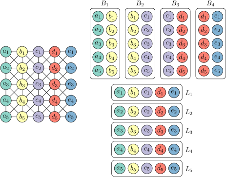
Figure 1: A width-2 layered path decomposition of the $5\times 5$ grid graph $G$.

Note that while layered pathwidth is at most pathwidth, pathwidth is not bounded by layered pathwidth. There are graphs—for example the $n\times n$ planar grid—that have unbounded pathwidth and bounded layered pathwidth. Thus upper bounds proved in terms of layered pathwidth are quantitatively stronger than those proved in terms of pathwidth. In addition, while having pathwidth at most $k$ is a minor-closed property, having layered pathwidth at most $k$ is not. For example, the $2\times n\times n$ grid graph has layered pathwidth at most $3$ but it has $K_{n}$ as a minor, and thus it has a minor of unbounded layered pathwidth. (Analogous statements hold for layered treewidth)

1.2 Linear Layouts

After introducing layered path decompositions, Bannister et al. [2, 3] set out to understand the relationship between track/queue/stack number and layered pathwidth.

A $t$-track layout of a graph $G$ is a partition of $V(G)$ into $t$ ordered independent sets $T_{1},\ldots,T_{t}$ (with a total order $\prec_{i}$ for each $T_{i}$, $i\in\{1,\ldots,t\}$) with no X-crossings. Here an X-crossing is a pair of edges $vw$ and $xy$ such that, for some $i,j\in\{1,\ldots,t\}$, $v,x\in T_{i}$ with $v\prec_{i}x$ and $w,y\in T_{j}$ with $y\prec_{j}w$. The minimum number of tracks in any $t$-track layout of $G$ is called the track number of $G$ and is denoted as $\operatorname{tn}(G)$. A $t$-track graph is a graph that has a $t$-track layout.

A stack (queue) layout of a graph $G$ consists of a total order $\sigma$ of $V(G)$ and a partition of $E(G)$ into sets, called stacks (queues), such that no two edges in the same stack (queue) cross; that is, there are no edges $vw$ and $xy$ in a single stack with $v\prec_{\sigma}x\prec_{\sigma}w\prec_{\sigma}y$ (nest; there are no edges $vw$ and $xy$ in a single queue with $v\prec_{\sigma}x\prec_{\sigma}y\prec_{\sigma}w$.). The minimum number of stacks (queues) in a stack (queue) layout of $G$ is the stack number (the queue number) of $G$ and is denoted as $\operatorname{sn}(G)$ ($\operatorname{qn}(G)$). A stack layout is also called a book embedding and stack number is also called book thickness and page number. An $s$-stack graph ($q$-queue graph) is a graph that has a stack (queue) layout with at most $s$ stacks ($q$ queues).

1.3 Summary of (Old and New) Results

A summary of known and new results on these rich relationships between layered pathwidth, queue number, stack number, and track number are outlined in Table 1. The first two rows show (the older results) that track number and queue number are tied; each is bounded by some function of the other [14, 15].

Queue-Number versus Track-Number
$\operatorname{qn}(G)\leq\operatorname{tn}(G)-1$	[14, Theorem 2.6]
$\operatorname{tn}(G)\leq 2^{O(\operatorname{qn}(G)^{2})}$	[15, Theorem 8]
Queue-Number versus Layered Pathwidth
$\operatorname{qn}(G)\leq 3\operatorname{lpw}(G)-1$	[14, Theorem 2.6][3, Lemma 9]
$\operatorname{qn}(G)=1\Rightarrow\operatorname{lpw}(G)\leq 2$	[18, Theorem 3.2][3, Corollary 7]
$\exists G:\operatorname{qn}(G)=2,\,\operatorname{lpw}(G)=\Omega((n/\log n)$	[16, Theorem 1.4]
Stack-Number versus Layered Pathwidth
$\operatorname{sn}(G)\leq 1\Rightarrow\operatorname{lpw}(G)\leq 2$	[3, Corollary 16]
$\exists G:\operatorname{sn}(G)=2,\,\operatorname{lpw}(G)=\Omega(\log n)$	($G$ is a binary tree plus an apex vertex)
$\exists G:\operatorname{sn}(G)=3,\,\operatorname{lpw}(G)=\Omega(n/\log n)$	[16, Theorem 1.5]
$\operatorname{sn}(G)\leq 4\operatorname{lpw}(G)$	Theorem 1
Track-Number versus Layered Pathwidth
$\operatorname{tn}(G)\leq 3\operatorname{lpw}(G)$	[3, Lemma 9]
$\operatorname{tn}(G)=1\Rightarrow\operatorname{lpw}(G)=1$	($G$ has no edges)
$\operatorname{tn}(G)\leq 2\Rightarrow\operatorname{lpw}(G)\leq 2$	($G$ is a forest of caterpillars)
$\operatorname{tn}(G)\leq 3\Rightarrow\operatorname{lpw}(G)\leq 4$	Theorem 2
$\exists G:\operatorname{tn}(G)=4,\,\operatorname{lpw}(G)=\Omega((n/\log n)$	[16, Theorem 1.5]

Table 1: Relationships between track number, queue number, stack number, and layered pathwidth.

The next group of rows relates queue number and layered pathwidth. Queue number is bounded by layered pathwidth [14]. Graphs with queue number 1 are arched-levelled planar graphs and have layered pathwidth at most 2. However, there are graphs with queue number 2 that are expanders; these graphs have pathwidth $\Omega(n)$ and diameter $O(\log n)$, so their layered pathwidth is $\Omega(n/\log n)$ [16]. Thus, layered pathwidth is not bounded by queue number.

The next group of rows examines the relationship between stack number and layered pathwidth. Graphs of stack number at most 1 are exactly the outerplanar graphs, which have layered-pathwidth at most 2 [3]. On the other hand, there are graphs of stack number 2 that have unbounded layered pathwidth [16]. Thus, in general, layered pathwidth is not bounded by stack number. Our first result, Theorem 1, shows that stack number is nevertheless bounded by layered pathwidth.

Theorem 1.

For every graph $G$, $\operatorname{sn}(G)\leq 4\operatorname{lpw}(G)$.

The final group of rows relates track number and layered pathwidth. Track number is bounded by layered pathwidth [3]. Layered pathwidth is bounded by track number when the track number is 1, or 2, but is not bounded by track number when the track number is 4 or more [3]. The question of what happens for track number 3 is stated as an open problem by Bannister et al. [3], who solved the special case when $G$ is bipartite and has track number 3. Our Theorem 2 solves this problem completely by showing that graphs with track number at most 3 have layered pathwidth at most 4.

Note that minor-closed classes that have bounded layered pathwidth have been characterized (as classes of graphs that exclude an apex tree as a minor) [9]. However, this result could not have been used to prove Theorem 2 since the family of 3-track graphs is not closed under taking minors.

Theorem 2.

Every graph $G$ that has $\operatorname{tn}(G)\leq 3$, has $\operatorname{lpw}(G)\leq 4$.

2 Proof of Theorem 1

Let $G$ be any graph, let $B=B_{1},\ldots,B_{p}$ be a path decomposition of $G$, and $\ell:V(G)\to\mathbb{Z}$ be a layering that obtains so that $B$ has layered width $\operatorname{lpw}(G)$ with respect to the layering $\ell$.

We may assume that $B$ is left-normal in the sense that, for every distinct pair $v,w\in V(G)$, $\min\{i\in\mathbb{Z}:v\in B_{i}\}\neq\min\{i\in\mathbb{Z}:w\in B_{i}\}$. It is straightforward to verify that any path decomposition can be made left-normal without increasing the layered width of the decomposition. We use the notation $v\prec_{B}w$ if $\min\{i\in\mathbb{Z}:v\in B_{i}\}<\min\{i\in\mathbb{Z}:w\in B_{i}\}$. Since $B$ is left-normal, $\prec_{B}$ is a total order.

For any edge $vw$ with $v\prec_{B}w$ we call $v$ the left endpoint of the edge and $w$ the right endpoint. We use the convention of writing any edge with endpoints $v$ and $w$ as $vw$ where $v$ is the left endpoint and $w$ is the right endpoint. With these definitions and conventions in hand, we are ready to proceed.

Proof of Theorem 1.

This proof is illustrated in Figure 2. Consider a left-normal path decomposition $B=B_{1},\ldots,B_{p}$ of $G$ and a layering $\ell:V(G)\to\mathbb{Z}$ such that $B$ has layered width at most $k$ with respect to $\ell$. Our goal is to construct a stack layout of $G$ using $4k$ stacks.

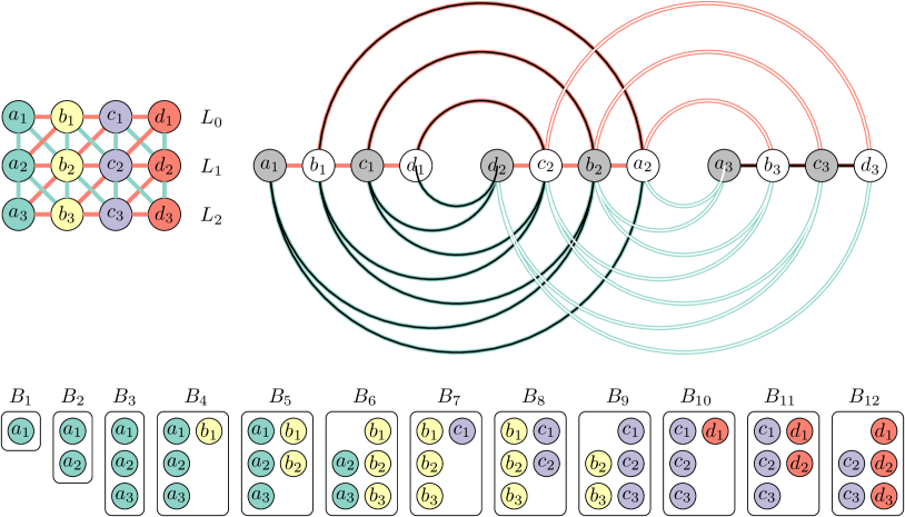
Figure 2: Colourings used in the proof of Theorem 1.

We first construct a total ordering $\prec_{\sigma}$ on the vertices of $G$, as follows:

1. If $v\in L_{i}$ and $w\in L_{j}$ with $i<j$, then $v\prec_{\sigma}w$.

2. If $v,w\in L_{i}$ with $v\prec_{B}w$ then

   1. $v\prec_{\sigma}w$ if $i$ is even; or

   2. $w\prec_{\sigma}v$ if $i$ is odd.

Next we define a colouring $\varphi:E(G)\to\{0,1\}\times\{0,1\}\times\{1,\ldots,k\}$ that determines a partition of the $E(G)$ into stacks. We begin with a (greedy) vertex $k$-colouring $\varphi:V\to\{1,\ldots,k\}$ so that, for any $i,j\in\mathbb{N}$, no two vertices in $B_{i}\cap L_{j}$ are assigned the same colour. This is easily done since, for each $j\in\mathbb{Z}$, the path decomposition $\langle B_{i}\cap L_{j}:i\in\mathbb{Z}\rangle$ has bags of size at most $k$.

We say that an edge $vw$ has positive slope if $\ell(v)=\ell(w)+1$ and has non-positive slope otherwise. We colour the edge $vw$ with the colour $\varphi(vw)=(a,b,c)$ where $a=\ell(v)\bmod 2$, $b\in\{0,1\}$ is a bit indicating whether $vw$ has positive ($b=1$) or non-positive ($b=0$) slope, and $c$ is the colour $\varphi(v)$ of the left endpoint $v$. This clearly uses only $2\times 2\times k=4k$ colours so all that remains is to show that $\sigma$ and the partition $P=\{\{vw\in E(G):\varphi(vw)=(a,b,c)\}:(a,b,c)\in\{0,1\}\times\{0,1\}\times\{1,\ldots,k\}\}$ is indeed a stack layout.

Consider any two distinct edges $vw,xy\in E(G)$ (whose left endpoints are $v$ and $x$, respectively). First observe that, if $\ell(v)\equiv\ell(x)\pmod{2}$ then either $\ell(v)=\ell(x)$ or $\ell(v)-\ell(x)\geq 2$. In the latter case, the only way in which $vw$ and $xy$ can cross with respect to $\prec_{\sigma}$ is if $\ell(v)+b=\ell(y)=\ell(w)=\ell(x)-b$ for some $b\in\{-1,1\}$. However, in this case, $vw$ has positive slope and $xy$ has non-positive slope, or vice-versa, so $\varphi(vw)$ and $\varphi(xy)$ differ in their second component. For example, we could have $\ell(x)=2$, $\ell(v)=0$, and $b=1$, in which case $\ell(y)=\ell(w)=1$, in which case $xy$ has positive slope and $vw$ has non-positive (in face, negative) slope.

Therefore, we only need to consider pairs of edges $xy$ and $vw$ where $\ell(v)=\ell(x)=i$. We assume, without loss of generality that $i$ is even and that $v\prec_{\sigma}x$. With these assumptions, there are only three cases in which $vw$ and $xy$ can cross:

1. $v\prec_{\sigma}x\prec_{\sigma}w\prec_{\sigma}y$.

   Since $\ell(v)=\ell(x)=i$ is even and $v\prec_{\sigma}x$, we have $v\prec_{B}x$ (by Property 2a) and $\ell(w)\geq i$ (by Property 1). If $\ell(w)=i$, then $v\prec_{B}x\prec_{B}w$ (by Property 2a), so $v$ and $x$ both appear in some bag $B_{j}$ and $\varphi(v)\neq\varphi(x)$, so $\varphi(vw)$ and $\varphi(xy)$ differ in their third component. If $\ell(w)=i+1$, then $w\prec_{\sigma}y$ implies that $\ell(y)\geq\ell(w)$ (by Property 1), which implies $\ell(y)=\ell(w)=i+1$, so $y\prec_{B}w$ (by Property 2b). We now have $v\prec_{B}x\prec_{B}y\prec_{B}w$ so $v$ and $x$ appear in a common bag $B_{j}$ and $\varphi(vw)$ and $\varphi(xy)$ differ in their third component.

2. $v\prec_{\sigma}y\prec_{\sigma}w\prec_{\sigma}x$. Since $v\prec_{\sigma}y$, $\ell(y)\geq\ell(v)=i$ (by Property 1). Similarly, since $y\prec_{\sigma}x$, $\ell(y)\leq\ell(x)=i$ (by Property 1). Therefore, $\ell(y)=i$, so $y\prec_{B}x$ (by Property 2a). This is not possible since, by definition, $x$ is the left endpoint of $xy$.

3. $y\prec_{\sigma}v\prec_{\sigma}x\prec_{\sigma}w$. Since $y\prec_{\sigma}x$, $ell(y)\leq\ell(x)=i$ (by Property 1). If $\ell(y)=i$ then, since $i$ is even, $y\prec_{B}x$ (by Property 2a) so it must be the case that $\ell(y)=i-1$. Since $x$ is the left endpoint of $xy$, $xy$ therefore has positive slope.

   Since $v\prec_{\sigma}w$ and $\ell(v)=i$ is even, we have $\ell(v)\leq\ell(w)$ (by Property 2a). Since $v$ is the left endpoint of $vw$, $vw$ therefore has non-positive slope. Therefore $\varphi(vw)$ and $\varphi(xy)$ differ in their second component.

Therefore, for any pair of edges $vw,xy\in E(G)$ that cross, $\varphi(vw)\neq\varphi(xy)$, so the partition $P$ is a partition of $V(G)$ into $4k$ stacks with respect to $\prec_{\sigma}$, as required. ∎

3 Proof of Theorem 2

Let $G$ be an edge-maximal $n$-vertex graph with $\operatorname{tn}(G)=3$. Here, $G$ is edge-maximal if adding any edge $e$ increases the track number to four or more. It is helpful to recall that $G$ is a planar graph that has a straight-line crossing-free drawing with the vertices of the track $T_{1}$ placed on the positive x-axis, the vertices of the track $T_{2}$ placed on the positive y-axis and the vertices of the track $T_{3}$ placed on the ray $\{(a,a):a<0\}$. See Figure 3.

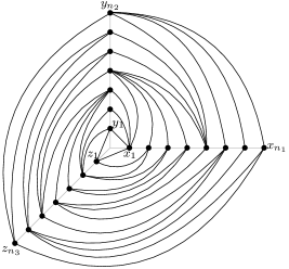
Figure 3: The standard planar embedding of a 3-track graph.

It will be easier to prove Theorem 2 for a weaker notion of layering. An $s$-weak layering of $G$ is a mapping $\ell:V(G)\to\mathbb{Z}$ with the property that, for every $vw\in E(G)$, $|\ell(v)-\ell(w)|\leq s$. The sets $L_{i}=\{v\in V(G):\ell(v)=i\}$ are called layers. The terms $s$-weak layered path decomposition and $s$-weak layered pathwidth of $G$, denoted $\operatorname{lpw}_{s}(G)$, are defined the same way as layered path decompositions and layered pathwidth, but with respect to $s$-weak layerings of $G$. The following result is easy (and well-known in the context of layered treewidth):

Lemma 1.

For any $s\in\mathbb{N}$, $\operatorname{lpw}(G)\leq s\cdot\operatorname{lpw}_{s}(G)$.

Proof.

By definition there exists an $s$-weak layering $\ell:V(G)\to N$ that defines layers $L_{i}=\{v\in V(G):\ell(v)=i\}$, $i\in\mathbb{Z}$, and a path decomposition $B_{1},\ldots,B_{p}$ of $G$ such that $|L_{i}\cap B_{j}|\leq\operatorname{lpw}_{s}(G)$ for each $i\in\mathbb{Z}$ and $j\in\{1,\ldots,p\}$.

Let $\ell^{\prime}(v)=\lfloor\ell(v)/s\rfloor$ for each $v\in V(G)$. For any edge $vw\in E(G)$, $\ell(v)-\ell(w)\leq s$, so $\ell^{\prime}(v)-\ell^{\prime}(w)\leq 1$, so $\ell^{\prime}$ is a layering of $G$. For each $i\in\mathbb{Z}$, the layer $L_{i}^{\prime}=\{v\in V(G):\ell^{\prime}(v)=i\}=\bigcup_{t=0}^{s-1}L_{is+t}$. Therefore, for each $i\in\mathbb{Z}$ and $j\in\{1,\ldots,p\}$, $L^{\prime}_{i}\cap B_{j}\leq\sum_{t=0}^{s-1}|L_{is+t}\cap B_{j}|\leq s\cdot\operatorname{lpw}_{s}(G)$. Thus, $\ell^{\prime}$ and $B_{1},\ldots,B_{p}$ are a layered path decomposition of $G$ of layered width at most $s\cdot\operatorname{lpw}_{s}(G)$, so $\operatorname{lpw}(G)\leq s\cdot\operatorname{lpw}_{s}(G)$. ∎

Let $T_{1},T_{2},T_{3}$ be a 3-track layout of $G$ with $T_{1}=\{x_{1},\ldots,x_{n_{1}}\}$, $T_{2}=\{y_{1},\ldots,y_{n_{2}}\}$, and $T_{3}=\{z_{1},\ldots,z_{n_{3}}\}$ and the total orders $\prec_{1},\prec_{2},\prec_{3}$ are implicit so that, for example $z_{i}\prec_{3}z_{j}$ if and only if $1\leq i<j\leq n_{3}$. In terms of Figure 3, this means that $x_{1},y_{1},z_{1}$ form the triangular face containing the origin and $x_{n_{1}},y_{n_{2}},z_{n_{3}}$ form the cycle on the boundary of the outer face. From this point onward, all track indices are implicitly taken “modulo 3” so that for any integer $j$, $T_{j}$ refers to the track $T_{j^{\prime}}$ with index $j^{\prime}=((j-1)\bmod 3)+1$.

The following observation follows from the fact that $G$ is edge-maximal.

Observation 1.

For any two vertices of $G$ on distinct tracks, say $x_{i}$ and $y_{j}$, at least one of the following conditions is satisfied (see Figure 4):

1. $x_{i}y_{j}\in E(G)$; or

2. there exists $x_{i^{\prime}}y_{j^{\prime}}\in E(G)$ with $i^{\prime}>i$ and $j^{\prime}<j$; or

3. there exists $x_{i}y_{j^{\prime}}\in E(G)$ with $j^{\prime}>j$.

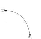
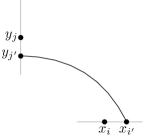
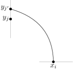
(1)	(2)	(3)

Figure 4: The three cases in Observation 1.

Theorem 2 is a consequence of the following lemma.

Lemma 2.

The edge-maximal 3-track graph $G$ with tracks $x_{1},\ldots,x_{n_{1}}$, $y_{1},\ldots,y_{n_{2}}$, and $z_{1},\ldots,x_{n_{3}}$ described above has a 2-weak layered path decomposition, $B_{1},\ldots,B_{p}$, with a layering $\ell$ of (layered) pathwidth $2$ in which

1. for each $i\in\{1,2,3\}$ and each $v\in T_{i}$, $\ell(v)\equiv i\pmod{3}$;

2. $B_{1}=\{x_{1},y_{1},z_{1}\}$;

3. $\ell(x_{1})=1$, $\ell(y_{1})=2$, and $\ell(z_{1})=3$;

4. $B_{p}=\{x_{n_{1}},y_{n_{2}},z_{n_{3}}\}$; and

5. $x_{n_{1}},y_{n_{2}},z_{n_{3}}$ appear in 3 distinct consecutive layers.

Before proving Lemma 2, we show how it implies Theorem 2. Since layered pathwidth is monotone with respect to the addition of edges, it is safe to assume (as Lemma 2 does) that $G$ is edge-maximal. By Lemma 2, therefore $G$ has $\operatorname{lpw}_{2}(G)\leq 2$ and therefore, by Lemma 1, $\operatorname{lpw}(G)\leq 4$.

Proof of Lemma 2.

If $|V(G)\leq 4$, then the result is trivial so assume from this point onward that $|V(G)\geq 5$. Next, suppose $V(G)$ contains a cut set $C=\{x_{i},y_{j},z_{k}\}$ having exactly one vertex in each track. Since $G$ is edge-maximal, $x_{i},y_{j},z_{k}$ form a cycle in $G$. Now, the subgraph $G_{1}$ of $G$ induced by $\{x_{1},\ldots,x_{i},y_{1},\ldots,y_{j},z_{1},\ldots,z_{k}\}$ is an edge-maximal graph with $\operatorname{tn}(G_{1})=3$ and we can inductively apply Lemma 2 to find a width-2 2-weak layered path decomposition of $G_{1}$ in which $x_{i},y_{j},z_{k}$ are in the last bag and are assigned to three consecutive distinct layers $r+1$, $r+2$, and $r+3$. Note that there are three possible assignments of $x_{i},y_{j},z_{k}$ to these three layers depending on the value of $r\bmod 3$. Suppose, without loss of generality, that $\ell(y_{j})=r+1$ (so $\ell(z_{k})=r+2$ and $\ell(x_{i})=r+3$.)

Next, consider the graph $G_{2}$ induced by $\{x_{i},\ldots,x_{n_{1}},y_{j},\ldots,y_{n_{2}},z_{k},\ldots,z_{n_{3}}\}$. We apply Lemma 2 inductively on $G_{2}$ relabelling tracks to ensure that in the resulting layered decomposition $\ell(y_{j})=1$, $\ell(z_{k})=2$ and $\ell(x_{i})=3$. We can now obtain a width-2 2-weak layered path decomposition of $G$ by joining the two decompositions. In particular, concatenating the sequence of bags for $G_{1}$ with the sequence of bags for $G_{2}$ gives a path decomposition of $G$ and adding $r$ to the indices of all layers in the layering of $G_{2}$ gives a 2-weak layering of $G$.

Thus, all that remains is to study the case where $G$ contains no cut set having exactly one vertex on each track. We claim that, in this case, $G$ contains the edge $x_{1}z_{2}$ or it contains the edge $z_{1}x_{2}$. Since $G$ is edge-maximal, this is obvious unless $n_{1}=n_{3}=1$ so that neither $z_{2}$ nor $x_{2}$ exist. However, since $|V(G)|\geq 5$, $n_{2}\geq 3$, so this would imply that $x_{1},z_{1},y_{2}$ is a cut set with one vertex on each track, since its removal separates all $y_{1}$ from $y_{3}$.

We will construct a path $P=v_{1},\ldots,v_{r}$, an example of which is illustrated in Figure 5(a). The first vertex of $P$ will be one of $x_{1},y_{1},z_{1}$ and the final three vertices are $x_{n_{1}}$, $y_{n_{2}}$, and $z_{n_{3}}$, though not necessarily in that order. The path $P$ will spiral in the sense that $v_{i}\in T_{i}$ for all $i\in\{1,\ldots,r\}$. Observe that this spiralling implies that the subsequence of vertices of $P$ on any track $T_{i}$ is increasing (getting further from the origin).

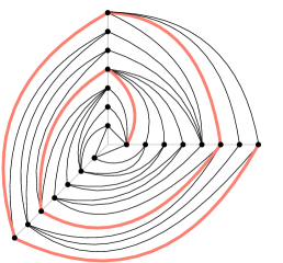
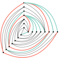
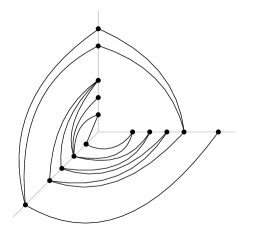
(a)	(b)	(c)

Figure 5: A three track graph $G$ with (a) the spiral curve, (b) edges spanning two layers highlighted, (c) the levelled planar graph $G-P$.

$P$ is constructed greedily: if $P$ has reached vertex $v_{k}$, it continues to the neighbouring vertex $v_{k+1}$ of $v_{k}$ with the highest index on track $T_{k+1}$ that is not yet in $P$. We will call this vertex $v_{k+1}$ the furthest neighbouring vertex of $v_{k}$. To see why this is always possible, recall that $P$ already contains an edge $v_{k-3},v_{k-2}$. Now, without loss of generality we can apply Observation 1 with $x_{i}=v_{k}$ and $y_{j}=v_{k-2}$, so there are three cases (see Figure 6):

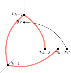
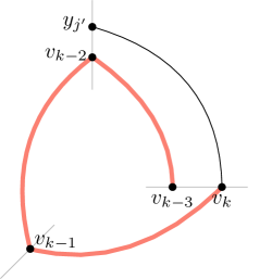
(1)	(2)	(3)

Figure 6: The path $P$ can always be extended.

1. $v_{k}v_{k-2}\in E(G)$. In this case $v_{k-2}$, $v_{k-1}$, and $v_{k}$ form a cycle in $G$. Then either $\{v_{k-2},v_{k-1},v_{k}\}=\{x_{n_{1}},y_{n_{2}},z_{n_{3}}\}$ or $\{v_{k-2},v_{k-1},v_{k}\}$ is a cut set with exactly one vertex in each track. In the former case, the path $P$ is complete. The latter case is excluded by the assumption that $G$ contains no such cut sets.

2. there exists an edge $x_{i^{\prime}}y_{j^{\prime}}\in E(G)$ with $i^{\prime}>i$ (i.e. $i^{\prime}>k$) and $j^{\prime}<j$ (i.e. $j^{\prime}<k-2$). This case is not possible, since this edge would cross $v_{k-3}v_{k-2}$.

3. there exists an edge $v_{k}y_{j^{\prime}}\in E(G)$ with $j^{\prime}>j$ (i.e. $j^{\prime}>k-2$). In this case, $P$ is extended by adding $v_{k+1}=y_{j^{\prime}}$.

Thus we have constructed the furthest vertex path $P=v_{1},\ldots,v_{r}$ whose first vertex is one of $x_{1},y_{1},z_{1}$ and whose last three vertices are $x_{n_{1}}$, $y_{n_{2}}$ and $z_{n_{3}}$ (not necessarily in order). We assign layers to the vertices of $P$ as follows: For each vertex $v_{i}$ on $P$, we set $\ell(v_{i})=i$. Note that this satisfies Conditions 3 and 5 of the lemma and also satisfies Condition 1 for the vertices of $P$. For each $t\in\{1,2,3\}$, any vertex $v\in T_{t}$ that is not in $P$ is assigned to the same layer as $v$’s immediate successor in $P\cap T_{t}$. This assignment satisfies Condition 1 for vertices not in $P$. Finally, we will prove that this gives a 2-weak layering of $G$. In other words, in the worst case, a vertex $v$ with $\ell(v)=i$ can only share an edge with vertex $u$ where $i-2\leq\ell(u)\leq i+2$. See Figure 5(b).

Any edge between $v$ and $w$ where neither $v$ nor $w$ is in $P$ will only span one layer. Any edge between any two vertices $v_{i}$ and $v_{j}$ where $v_{i},v_{j}\in P$, will span only one layer if $j=i\pm 1$. This would mean that $v_{i}v_{j}$ is an edge in the graph $G$ and that this edge was used to construct our furthest vertex path $P$. If $j\neq i\pm 1$, then there are two cases:

1. $j=i\pm 2$ Such an edge is possible, and allowed since it spans only two layers.

2. $j=i\pm 4$ Such an edge cannot exist since it would contradict our greedy path constructing algorithm. If the edge $v_{i}v_{i+4}$ (or the edge $v_{i-4}v_{i}$) existed then the edge $v_{i}v_{i+1}$ ($v_{i-4}v_{i-3}$ ) would not have been added to $P$.

Any edge between $v$ and $w$ where $v\in P$ and $w\not\in P$ will be one of 7 types (see Figure 7). Without loss of generality, assume the spiral is travelling from $T_{1}$ to $T_{2}$ to $T_{3}$. Let $x_{i}$ be a vertex on the constructed path $P$. First, we look at the possible cases for an edge between $x_{i}$ with $\ell(x_{i})=m$ and $y_{j}$ where $y_{j}\notin P$.

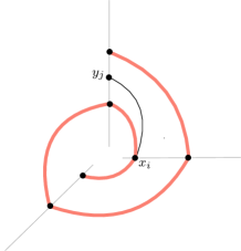
1

2

3

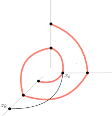
4

5

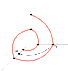
6

7

Figure 7: The edge between a vertex $x_{i}$ and a vertex $y_{j}$ or $z_{k}$ cannot span more than 2 layers

1. $\ell(y_{j})=m+3n$ where $n\geq 1$. This edge cannot exist since it would contradict our greedy path constructing algorithm.

2. $\ell(y_{j})=m+1$. This edge will only span one layer.

3. $\ell(y_{j})=m+1-3n$ where $n\geq 1$. This edge cannot exist, since it would create a crossing with the edge $v_{m-3}v_{m-2}$.

Second, we look at the possible cases for an edge between $x_{i}$ with $\ell(x_{i})=m$ and $z_{k}$ where $z_{k}\notin P$.

1. $\ell(z_{k})=m+2+3n$ where $n\geq 1$. This edge cannot exist, since it would create a crossing with the edge $v_{m+2}v_{m+3}$.

2. $\ell(z_{k})=m+2$. This edge spans exactly two layers.

3. $\ell(z_{k})=m-1$. This edge will only span one layer.

4. $\ell(z_{k})=m-1-3n$ where $n\geq 1$. This edge cannot exist, since it would create a crossing with the edge $v_{m-4}v_{m-3}$.

Next, we will need a notion of levelled planar graphs. The class of levelled planar graphs was introduced in 1992 by Heath and Rosenberg [18] in their study of queue layouts of graphs. A levelled planar drawing of a graph is a straight-line crossing-free drawing in the plane, such that the vertices are placed on a sequence of parallel lines (called levels), where each edge joins vertices in two consecutive levels. A graph is levelled planar if it has a levelled planar drawing. (This is a well studied model for planar graph drawing, known as a Sugiyama-style drawing [19, 4, 17, 5].)

Now, consider the graph $G-P$ obtained by removing the vertices of $P$ from $G$ (see Figure 5(c)). We claim that this graph is a levelled planar graph in which the levels of the vertices are given by the layering $\ell$ defined above. (Recall that the edges of $G$ spanning two layers all have at least one endpoint in $P$.) Refer to Figure 8. One way to see this is to imagine $G$ as being drawn with its vertices on the three vertical edges of the surface of a triangular prism so that $x_{1},y_{1},z_{1}$ are the vertices of one triangular face and $x_{n_{1}},y_{n_{2}},z_{n_{3}}$ are the vertices of the other triangular face. Now, if we remove the triangular faces of this prism, cut it along the embedding of $P$, and unfold the resulting surface so that it lies in the plane, then we obtain a drawing of $G-P$ in which the vertices lie on a set of parallel lines and in which the edges only join vertices on two consecutive lines. This gives the desired levelled planar drawing of $G-P$.

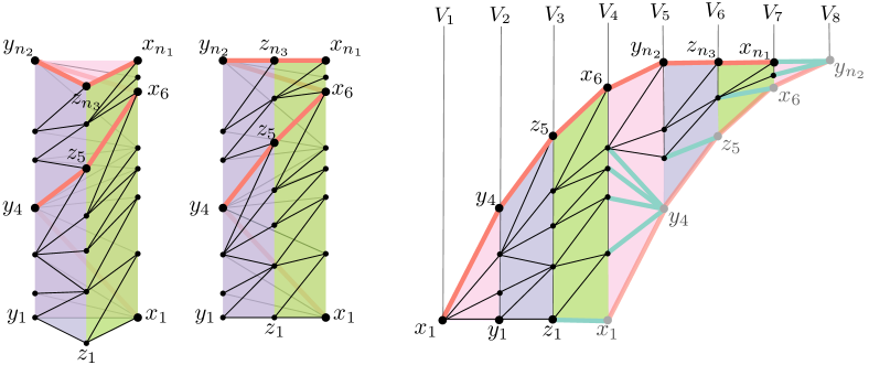
Figure 8: Cutting a prism along $P$ to obtain a levelled planar drawing of $G-P$.

By a result of Bannister et al. [3, Proof of Theorem 5], $G-P$ has a layered path decomposition $B_{1},\ldots,B_{p}$ of width 1 using the layering $\ell$ defined above. If we add the vertices of $P$ to every bag of this decomposition we obtain a width-2 2-weak layered path decomposition of $G$. Finally, to satisfy Conditions 2 and 4 of the lemma, we prepend a bag $B_{0}=\{x_{1},y_{1},z_{1}\}$ and append a bag $B_{p+1}=\{x_{n_{1}},y_{n_{2}},z_{n_{3}}\}$. ∎

4 Conclusions

We have presented two results on layered pathwidth that help complete our understanding of the relationship between layered pathwidth, stack number, and track number. Graphs of bounded layered pathwidth include grids and certain types of intersection graphs. Theorem 1, for example, implies that unit-disk graphs with maximum clique size $k$ have stack number $O(k)$ since they have been shown to have $O(k)$ layered pathwidth [2, 3].

We conclude this discussion by remarking that upper bounds on the stack number of graphs of bounded layered treewidth are not yet known, and present a challenging avenue for further study. For example, $k$-planar graphs are known to have layered treewidth $O(k)$ [10, Theorem 3.1]. Therefore, bounding stack number by a function of layered treewidth would imply that $k$-planar graphs have bounded stack-number. It is still unknown whether $k$-planar graphs have bounded stack-number except in the case $k=1$ [6, 1].

References

- [1] Md. Jawaherul Alam, Franz J. Brandenburg, and Stephen G. Kobourov. On the book thickness of 1-planar graphs. CoRR, abs/1510.05891, 2015.
- [2] Michael J. Bannister, William E. Devanny, Vida Dujmović, David Eppstein, and David R. Wood. Track layout is hard. In Yifan Hu and Martin Nöllenburg, editors, Graph Drawing and Network Visualization - 24th Int. Symposium, GD 2016, volume 9801 of Lecture Notes in Computer Science, pages 499–510. Springer, 2016.
- [3] Michael J. Bannister, William E. Devanny, Vida Dujmović, David Eppstein, and David R. Wood. Track layouts, layered path decompositions, and leveled planarity. Algorithmica, pages 1–23, July 2018.
- [4] Oliver Bastert and Christian Matuszewski. Layered drawings of digraphs. Drawing Graphs, Methods and Models, 2025:87–120, 2001.
- [5] Giuseppe Di Battista, Peter Eades, Roberto Tamassia, and Ioannis G. Tollis. Layered drawings of digraphs. Graph Drawing: Algorithms for the Visualization of Graphs, pages 265–302, 1999.
- [6] Michael A. Bekos, Till Bruckdorfer, Michael Kaufmann, and Chrysanthi N. Raftopoulou. The book thickness of 1-planar graphs is constant. Algorithmica, 79(2):444–465, 2017.
- [7] Marthe Bonamy, Cyril Gavoille, and Michal Pilipczuk. Shorter labeling schemes for planar graphs. In Shuchi Chawla, editor, Proceedings of the 2020 ACM-SIAM Symposium on Discrete Algorithms, SODA 2020, Salt Lake City, UT, USA, January 5-8, 2020, pages 446–462. SIAM, 2020.
- [8] Michal Debski, Stefan Felsner, Piotr Micek, and Felix Schröder. Improved bounds for centered colorings. In Shuchi Chawla, editor, Proceedings of the 2020 ACM-SIAM Symposium on Discrete Algorithms, SODA 2020, Salt Lake City, UT, USA, January 5-8, 2020, pages 2212–2226. SIAM, 2020.
- [9] Vida Dujmović, David Eppstein, Gwenaël Joret, Pat Morin, and David R. Wood. Minor-closed graph classes with bounded layered pathwidth. CoRR, abs/1810.08314, 2018.
- [10] Vida Dujmović, David Eppstein, and David R. Wood. Structure of graphs with locally restricted crossings. SIAM J. Discrete Math., 31(2):805–824, 2017.
- [11] Vida Dujmović, Louis Esperet, Gwenaël Joret, Cyril Gavoille, Piotr Micek, and Pat Morin. Adjacency labelling for planar graphs (and beyond). CoRR, abs/2003.04280, 2020.
- [12] Vida Dujmović, Louis Esperet, Gwenaël Joret, Bartosz Walczak, and David R. Wood. Planar graphs have bounded nonrepetitive chromatic number. CoRR, abs/1904.05269, 2019.
- [13] Vida Dujmović, Gwenaël Joret, Piotr Micek, Pat Morin, Torsten Ueckerdt, and David R. Wood. Planar graphs have bounded queue-number. In David Zuckerman, editor, 60th IEEE Annual Symposium on Foundations of Computer Science, FOCS 2019, Baltimore, Maryland, USA, November 9-12, 2019, pages 862–875. IEEE Computer Society, 2019.
- [14] Vida Dujmović, Pat Morin, and David R. Wood. Layout of graphs with bounded tree-width. SIAM J. Comput., 34(3):553–579, 2005.
- [15] Vida Dujmović, Attila Pór, and David R. Wood. Track layouts of graphs. Discrete Mathematics & Theoretical Computer Science, 6(2):497–522, 2004.
- [16] Vida Dujmović, Anastasios Sidiropoulos, and David R. Wood. Layouts of expander graphs. Chicago J. Theor. Comput. Sci., 2016, 2016.
- [17] Patrick Healy and Nikola S. Nikolov. Hierarchical drawing algorithms. Handbook on Graph Drawing and Visualization, pages 409–453, 2013.
- [18] Lenwood S. Heath and Arnold L. Rosenberg. Laying out graphs using queues. SIAM J. Comput., 21(5):927–958, 1992.
- [19] K. Sugiyama, S. Tagawa, and M. Toda. Methods for visual understanding of hierarchical system structures. IEEE Trans. Systems Man Cybernet., 11(2):109–125, 1981.