$\mathcal{Q}$System: bitwise representation for quantum circuit simulations

Abstract

We present $\mathcal{Q}$System, an open-source platform for the simulation of quantum circuits focused on bitwise operations on a Hashmap data structure storing quantum states and gates. $\mathcal{Q}$System is implemented in C++ and delivered as a Python module, taking advantage of the C++ performance and the Python dynamism. The simulator’s API is designed to be simple and intuitive, thus streamlining the simulation of a quantum circuit in Python. The current release has three distinct ways to represent the quantum state: vector, matrix, and the proposed bitwise. The latter constitutes our main results and is a new way to store and manipulate both states and operations which shows an exponential advantage with the amount of superposition in the system’s state. We benchmark the bitwise representation against other simulators, namely Qiskit, Forest SDK QVM, and Cirq.

Keywords: Quantum Computation, Quantum Circuit Simulation, Python

1 Introduction

Quantum computation is a new paradigm of computing which uses quantum phenomena, such as superposition and entanglement, to efficiently tackle classes of problems out of reach for classical computers. Since the seminal works of Shor [1] and Grover [2] showcasing relevant quantum algorithms with advantage over their classical counterparts, the field has seen significant efforts both in theory and experiments [3, 4, 5]. The search for other possible algorithms is a very active field as well their implementations or simulations [6, 7, 8, 9, 10].

In this scenario, the simulation of quantum dynamics and small quantum circuits in a classical computer is of central importance. These may be used to validate computing models [11, 12], simulate physical theories [13, 14, 15, 16, 17] and even to define the break-even point, when quantum computers match what is classically achievable [18]. To this end, several quantum circuit simulators have been developed in the past years, both from academic and industrial players [19, 20, 21, 22, 23, 24, 25, 26]. In common to these approaches is the drive to improve the memory and time cost of such simulations. Owing to the predicted exponential scaling of these resources with the number of qubits, efficiency is at the core of previous implementations, which try to push the boundary of what can be simulated [27, 28, 29].

Here we introduce a new approach to quantum circuit simulations that can display exponential advantage over other simulators. Our approach is based on Hashmaps to store quantum states and gates, and uses bitwise operations to implement gates. For quantum states that can be well described by a small, yet unknown set of basis states, we argue that the small number of keys in their respective Hashmap leads to an exponential speedup. This is further observed in benchmark tests against a number of popular simulators. We implement this approach on $\mathcal{Q}$System, a quantum circuit simulator which was developed to support the study and construction of quantum algorithms, quantum protocols, error correction codes and other quantum applications that can be described as a quantum circuit. The $\mathcal{Q}$System’s API is developed as a Python module, wrapping a C++ code, with methods resembling common quantum computing language/terminology, making it easy the transcribe any quantum circuit. Besides the bitwise representation, $\mathcal{Q}$System also provides a vector representation of pure quantum states and a density matrix representation for simulations of circuits with quantum errors, including predefined methods for quantum error correction.

The remainder of this paper is organized as follows: In Section 2, a brief introduction to quantum computation is given. Section 3 presents the $\mathcal{Q}$System simulator and the bitwise representation is described in Section 4. The benchmarks are discussed in Section 5 and our concluding remarks are given in Section 6.

2 Quantum computing

The quantum computing basic operating unit is the quantum bit, or qubit. Like the classical bit, the qubit can be at the state 0, represented by $\ket{0}$, and 1, represented by $\ket{1}$, which form a basis for the qubit description and manipulation. However, unlike the classical bit, a qubit can also be described as a convex sum (or superposition) of its basis states represented as $\alpha\ket{0}+\beta\ket{1}$, with $\alpha$ and $\beta\in\mathbb{C}$ and $|\alpha|^{2}+|\beta|^{2}=1$  [30]. Measuring the qubit in this computational basis destroys this superposition and collapses the quantum state to either $\ket{0}$ or $\ket{1}$ with probabilities $|\alpha|^{2}$ and $|\beta|^{2}$, respectively. Therefore a $2$-dimensional normalized complex vector can be used to represent the state of a qubit. This is often the path used for numerical simulations of quantum mechanics.

For an $n$-qubit system, the above ideas can be generalized and a unit vector in $\mathbb{C}^{2^{n}}$ is used to represent the quantum state. It is immediately clear that the dimension of the vector space scales exponentially with system size, rendering simulations of systems larger than a few dozen qubits intractable.

The computational basis is defined by a set of basis states where each qubit is in either the $\ket{0}$ or $\ket{1}$ states (no superpositions allowed in this basis states). For a $3$-dimensional system these would be

$$\matrix{\ket{0}=\left|000\right),&\ket{1}=\left|001\right),&\ket{2}=\left|010\right),\cr\ket{3}=\left|011\right),&\ket{4}=\left|100\right),&\ket{5}=\left|101\right),\cr\ket{6}=\left|110\right),&\ket{7}=\left|111\right),}$$ (1)

where we have introduced the notation $\ket{n}$ as a useful representation of the computational basis states in terms of integer numbers and $\left|\cdot\right)$ to represent these in terms of individual qubit states. An arbitrary system state, $\ket{\psi}=\sum_{i=0}^{2^{n}-1}\alpha_{i}\ket{i}$, can the be represented as a $2^{n}-1$ dimensional unit vector with $i$-component given by $\alpha_{i}$. In $\mathcal{Q}$System this will be called a vector representation.

For systems with classical error, the quantum state is described by the so-called density matrix. If the system has a classical probability $p_{i}$ of being found in a given quantum state $\ket{\psi_{i}}$, its density matrix is $\rho=\sum_{i}p_{i}\ket{\psi_{i}}\mkern-7.0mu\bra{\psi_{i}}$. In a numerical implementation this can be mapped to a matrix representation where $\ket{\psi}\mkern-7.0mu\bra{\phi}$ is the outer product of a column vector $\ket{\psi}$ and a row vector $\ket{\phi}$. Such description allows one to include errors in the computation and study, e.g., quantum error correction schemes [30]. In $\mathcal{Q}$System this will be called a matrix representation.

Operations on the system state can take three forms, quantum gates, quantum channels and measurements. Quantum gates are unitary operations acting on a subset of the qubits. These can be represented by $2^{n}\times 2^{n}$ matrices. As an example, the Hadamard gate acting on states $\ket{0}$ and $\ket{1}$ of a single qubit system is given by

$$H\ket{0} =\frac{1}{\sqrt{2}}\left[\matrix{1&1\cr 1&-1}\right]\left[\matrix{1\cr 0}\right]=\frac{1}{\sqrt{2}}\left[\matrix{1\cr 1}\right] =\frac{1}{\sqrt{2}}(\ket{0}+\ket{1})\equiv\ket{+}$$ (2)

$$H\ket{1} =\frac{1}{\sqrt{2}}\left[\matrix{1&1\cr 1&-1}\right]\left[\matrix{0\cr 1}\right]=\frac{1}{\sqrt{2}}\left[\matrix{1\cr-1}\right] =\frac{1}{\sqrt{2}}(\ket{0}-\ket{1})\equiv\ket{-}$$ (3)

In quantum computation, the most widely used measurement type is the projective measurement on the eigenbasis of a given observable, $\mathcal{O}$, and the measurement statistics determines the outcome of a given computation. This measurement projects the state, $\rho$, into one of the basis states with a probability given by $\Tr(\rho\mathcal{O})$.

The last operation that can be performed is a quantum channel. These are used to account for errors in the computation and lead to classical uncertainty in the final state and can be described by $\rho^{\prime}=\sum_{i}K_{i}\rho K_{i}^{\dagger}$, where $K_{i}$ are the Kraus operators satisfying $\sum_{i}K_{i}^{\dagger}K_{i}=\mathbb{1}$ for trace-preserving channels. This describes non-unitary evolutions and is the standard way to study error propagation and quantum error correction. We refer the interested reader to References [31, 30] for a detailed discussion.

Naturally, there is a large set of more specific tools, protocols and algorithms in quantum computation, many of which are implemented in $\mathcal{Q}$System. In the following we will introduce the $\mathcal{Q}$System  simulator, focusing on the bitwise representation and on a few of its methods. The complete list of methods is available in Reference [32].

3 The Simulator

$\mathcal{Q}$System  is a quantum circuit simulator for Python designed with three central concepts: (i) efficiency, (ii) simple methods and (iii) general use. Altough the simulator is delivered as a Python module, it was developed in C++ for improved efficiency. The software SWIG [33] was used to wrap the C++ code and generate an interface with the Python interpreter. This is done by a configuration file and no modification is needed in the C++ source code. With this, the core C++ code is independent of the Python library and can be used standalone with few modifications. Our main result, the bitwise representation is a powerful tool to improve efficiency in some cases, and will be discussed in Section 4.

To design a toolbox with methods that are simple and intuitive to call, we tried to keep the coding as close as possible to the natural use of the English language when referring to a given tool. As an example, applying a controlled phase gate of $\theta$ to target qubit $t$, with control qubits $c_{1}$ and $c_{2}$ is done with the function cphase$\left(\theta,t,\left[c_{1},c_{2}\right]\right)$.

Typical quantum computing core operations have been implemented in $\mathcal{Q}$System, as well as more sophisticated functions, such as quantum Fourier transform [34] and some quantum error correction protocols [31]. The simulator can thus be used for a number of applications, including quantum algorithms, quantum protocols and error correcting codes. The evolution of a state is described in two classes: (i) the QSystem class, which names the simulator, holds and controls the quantum state, applying quantum gates and performing measurements; and (ii) the Gate class, used to create quantum gates different from the default set of gates in the QSystem class.

Representation.

The $\mathcal{Q}$System simulator has three forms to represent the quantum state, the bitwise and vector for pure states and matrix for simulations of noisy systems. The bitwise representation is detailed in Section 4. As the vector and matrix representation are a straight forward implementation of state vectors and density matrices using sparse matrices (see Section 2), we will not describe these representations here. For linear algebra operations, such as matrix multiplication and tensor product, we used the template-based C++ Armadillo library [35, 36].

Quantum gates.

The QSystem class has several methods to apply quantum gates. Single-qubit gates are summarized in Table 1 and Multiple-qubits gates in Table 2. Other predefined methods include qft(), used to apply a Quantum Fourier Transformation, and apply() used to apply a user-defined quantum gate, created by the Gate class.

Table 1: Single-qubit gates predefined in QSystem. The last column refers to QSystem’s method and the required parameters for implementations.

Gate name	Matrix form	Method
Pauli X	$\left[\matrix{0&1\cr 1&0}\right]$	evol(’X’, qubitID)
Pauli Y	$\left[\matrix{0&-i\cr i&0}\right]$	evol(’Y’, qubitID)
Pauli Z	$\left[\matrix{1&0\cr 0&-1}\right]$	evol(’Z’, qubitID)
Hadamard	$\frac{1}{\sqrt{2}}\left[\matrix{1&1\cr 1&-1}\right]$	evol(’H’, qubitID)
S Gate	$\left[\matrix{1&0\cr 0&i}\right]$	evol(’S’, qubitID)
T Gate	$\left[\matrix{1&0\cr 0&e^{\frac{i\pi}{4}}}\right]$	evol(’T’, qubitID)
X rotation	$\left[\matrix{\cos\frac{\theta}{2}&-i\sin\frac{\theta}{2}\cr-i\sin\frac{\theta}{2}&\cos\frac{\theta}{2}}\right]$	rot(’X’, $\theta$, qubitID)
Y rotation	$\left[\matrix{\cos\frac{\theta}{2}&-\sin\frac{\theta}{2}\\ \sin\frac{\theta}{2}&\cos\frac{\theta}{2}}\right]$	rot(’Y’, $\theta$, qubitID)
Z rotation	$\left[\matrix{-e^{i\theta/2}&0\\ 0&e^{i\theta/2}}\right]$	rot(’Z’, $\theta$, qubitID)
U3 gate	$\left[\matrix{\cos\frac{\theta}{2}&-e^{i\lambda}\sin\frac{\theta}{2}\cr e^{i\phi}\sin\frac{\theta}{2}&e^{i(\lambda+\phi)}\cos\frac{\theta}{2}}\right]$	u3($\theta$, $\phi$, $\lambda$, qubitID)
U2 gate	$\frac{1}{\sqrt{2}}\left[\matrix{1&-e^{i\lambda}\\ e^{i\phi}&e^{i(\lambda+\phi)}}\right]$	u2($\phi$, $\lambda$, qubitID)
U1 gate	$\left[\matrix{1&0\\ 0&e^{i\lambda}}\right]$	u1($\lambda$, qubitID)

Table 2: Multiple-qubits gates predefined in QSystem. The last column refers to QSystem’s method used to apply it.

Gate name	Circuit form	Method
CNOT		cnot(targetQubitID, [ctrlQubitID, $\dots$])
CPhase		cphase($e^{\theta}$, targetQubitID, [ctrlQubitID, $\dots$])
SWAP		swap(qubitIDa, qubitIDb)

The Gate Class has four static methods to create a custom gate:

• Gate.from_matrix([$U_{00}$, $U_{01}$, $U_{10}$, $U_{11}$]), used to create a single-qubit gate from an input matrix.

• Gate.from_sp_matrix(size, row, column, value), used to create an $n$-qubit gate from a sparse matrix. The sparse matrix $U$ is split into three parts, row, column, and value, where

  $$U(\texttt{row}\texttt{[i]},\texttt{column}\texttt{[i]})=\texttt{value}\texttt{[i]}.$$ (4)

• Gate.from_func(func, $n$), used to create an $n$-qubit gate from a Python function. Considering a Python function func() that has a single unsigned integer as input and output, the matrix that represents the created gate is defined as

  $$\sum_{i=0}^{2^{n}-1}\ket{\texttt{func(}i\texttt{)}}\mkern-7.0mu\bra{i}.$$ (5)

• Gate.cxz_gate(stabilizer, [ctrlQubitID, $\dots$]), used to create a syndrome measurement gate, used in quantum stabilizer codes [31].

For vector and matrix representations we use late evaluation to reduce the time taken on matrix multiplications. When a gate is applied, the request is registered in a list where each item describes the gates acting on each qubit. When a new computation depends on any of its pending results, these gates are applied generating the matrix for the unitary transformation.

Measurement.

The simulator is able to perform measurements in the computational basis (equivalent to a Pauli Z measurement) using the methods measure(qubitID) and measure_all(). Measurements on other basis can be achieved by pre-measurement rotations, e.g. a Pauli X measurement is performed by applying a Hadamard gate before the measurement.

When a qubit is measured it collapses on the computational base state corresponding to the measurement result. The qubit can be subsequently used and measured again. Measurement results are stored in a list accessible via the method bits(). Each element of this list holds the last measurement outcome of each qubit, where the possible values are 0, 1, or None for unmeasured qubits.

Quantum errors.

Quantum errors can be simulated within the matrix representation. Predefined error channels are:

• Bit flip, flip(’X’, $\rho$, $p$): $\mathcal{E}(\rho|p)=(1-p)\rho+p(X\rho X)$.

• Phase flip, flip(’Z’, $\rho$, $p$): $\mathcal{E}(\rho|p)=(1-p)\rho+p(Z\rho Z)$.

• Bit-phase flip, flip(’Y’, $\rho$, $p$): $\mathcal{E}(\rho|p)=(1-p)\rho+p(Y\rho Y)$.

• Amplitude damping, amp_damping($\rho$, $p$):
  $\mathcal{E}(\rho|p)=\left[\matrix{1&0\cr 0&\sqrt{1-p}}\right]\rho\left[\matrix{1&0\cr 0&\sqrt{1-p}}\right]+\left[\matrix{0&0\cr\sqrt{p}&0}\right]\rho\left[\matrix{0&\sqrt{p}\cr 0&0}\right]$.

• Depolarizing channel, dpl_channel($\rho$, $p$):
  $\mathcal{E}(\rho|p)=\left(1-\frac{3p}{4}\right)\rho+\frac{p}{4}(X\rho X+Y\rho Y+Z\rho Z)$.

Where $p$ is the probability that an error occurs.

4 The bitwise representation

Bitwise operations.

The bitwise operations underlying the bitwise representation presented here are logical and shift operations on a set of individual bits of a bit string. These treat a given number in its binary representation and operate on it bit-by-bit, and will be used, e.g., to transform one basis state to another. Logical bitwise operations used here include AND (“$\wedge$”), OR (“$|$”), and XOR (“$\oplus$”). To illustrate these, consider the following operation $\ket{3}$ OR $\ket{5}$ in a 4-qubit simulator. This gives

$$\matrix{&\ket{3}\quad(\left|0011\right))\cr\mathrm{OR}&\ket{5}\quad(\left|0101\right))\cr\hline\cr\cr=&\ket{7}\quad(\left|0111\right))}.$$ (6)

The AND (“$\wedge$”) is used to apply a selection mask to the bit string. This mask is usually given by numbers of the form

$$2^{n}\equiv 01\overbrace{0\dots 0}^{n},$$ (7)

with the associated bit string consisting of a bit 1 at position $n+1$ (from right to left) and all other bits 0. The mask can also be given by numbers of the form

$$2^{n}-1\equiv 0\overbrace{1\dots 1}^{n},$$ (8)

with a bit string consisting of bits 1 for positions to the right of $n$ and all other bits set to 0. For example, if we what to select the first three qubits of $\ket{22}$, we use the operation $\ket{22}\wedge(2^{3}-1)$, that gives

$$\matrix{&\ket{22}&(\left|10110\right))\cr\mathrm{AND}&2^{3}-1&(00111)\cr\hline\cr\cr=&\ket{6}&(\left|00110\right))}.$$ (9)

$\mathcal{Q}$System indexes qubits from left to right starting at 0.

The XOR (“$\oplus$”) is used flip a bit. This way, if we what to apply a Pauli X gate on the $n$-th qubit of the estate $\ket{i}$ we use the operation $\ket{i}\oplus 2^{n}\equiv X_{n}\ket{i}$, e.g., $\ket{10}\oplus 2^{2}$ gives

$$\matrix{&\ket{9}&(\left|1001\right))\cr\mathrm{XOR}&2^{2}&(0100)\cr\hline\cr\cr=&\ket{14}&(\left|1101\right))}.$$ (10)

Shift operations move the entire bit string sideways a given number of times and can be Shift left (“$\ll$”) and Shift right (“$\gg$”). Apply a Shift left adds zeros to the right side of the bit string, multiplying the number by $2^{n}$, e.g., $7\ll 2=28$. It is useful to create masks, e.g., $(1\ll n)-1=2^{n}-1$ creates a mask to select the first $n$ bits, and $1\ll n=2^{n}$ can be used to flip the $n$-th bit. We can rewrite Equation (9) as $\ket{22}\wedge((1\ll 3)-1)=\ket{6}$ and Equation (10) as $\ket{10}\oplus(1\ll 2)=\ket{14}$. The Shift right consumes the first bits, dividing (entire division) it by $2^{n}$, e.g., $7\gg 2=1$.

State and gate representations.

The bitwise representation uses Hashmaps to represent pure states and quantum gates [37]. While Hashmaps require heavy memory use, the concise way to represent sparse states and gates allows them to have significant gain in time, as will be seen in Section 5. Pure states will be represented by the Hashmap bwQubits, which takes unsigned integers as key and maps it to a complex number. The key represents a base vector $\ket{i}$ of the system and the complex number its amplitude $\alpha_{i}$, with the equivalence

$$\ket{\psi}=\sum_{i=0}^{2^{n}-1}\alpha_{i}\ket{i}\equiv\sum_{\textrm{key}\,\in\,\texttt{bwQubits}}\texttt{bwQubits}[\textrm{key}]\ket{\textrm{key}}.$$ (11)

As with the sparse matrix representation, this representation only stores the nonzero elements of the vector state. An important advantage is that the Hashmap size is independent of the number of qubits, e.g. the state $\ket{5}$ can represent the states $\left|101\right)$, $\left|0101\right)$, and $\left|0\dots 00101\right)$ by simply changing the number of qubits, with no additional memory required. This is at the root of the performance gains obtained with the bitwise representation. The exponentially growing system size with the number of qubits does not imply an exponential increase in memory used to store the key. The Hashmap memory needed grows only as more basis states are required to describe the system. As we will see below, the time necessary to operate on the system will also depend on the Hashmap size, not on the number of qubits. This can generate significant speedups.

The evolution of a pure state is given by a unitary gate $U$. We represent these with the Hashmap bwGate, which takes an unsigned integer as key and has a set of pairs as the mapped value. Each pair in this set is given by a complex number and an unsigned integer. The key represents a base vector the gate is acting on and the set of pairs represents each output base state and it’s associate amplitude, according to

$$U\ket{i}\equiv\sum_{(\alpha_{j},j)\,\in\,\texttt{bwGate}[i]}\alpha_{j}\ket{j}.$$ (12)

For an arbitrary gate $U$ prepared as bwGate, Algorithm 1 describes it’s application to a bwQubits state. The algorithm iterates over the basis states present in bwQubits’ superposition, applying the gate to each of them and constructing the final state.

Algorithm 1: arbitrary gate.

Let size be the number of qubits in a given system we want to evolve, and bwGateSize the number of qubits this gate acts on. The current version of $\mathcal{Q}$System  only allows user-defined multi-qubit gates applied to neighboring qubits, where qubitID labels the first affected qubit. We remark that more general gates would have no additional computational complexity and are planned for future versions. We now look into each step of the pseudocode in Algorithm 1. The algorithm starts creating an empty instance of the bitwise Hashmap representation (line 1) and iterates over all values of bwQubits’ key (line 1). The key is split into three parts: $x$, $y$ and $z$. Variables $x$ and $z$ hold the qubit values to the left and right, respectively, of the qubits affected by the gate (lines 1 and 1). Variable $y$ holds the value of the qubits the gate will operate on. As each gate is defined to operate on a specific system dimension, $y$ must hold the state information on the far-right bits (lines 1 and 1).

With the split key, we iterate over the bwGate[$y$] (line 1), applying $U\ket{y}$. Variables $x$, $i$ (shifted back to qubitID), and $z$ are concatenated with a bitwise OR (line 1), with variable xiz representing one output key of $U\ket{y}$. The output state is updated according to Eq.(12) (line 1) and any key for which the state has zero amplitude is removed from the Hashmap (lines 1 and 1). Finally the output of the gate is returned (line 1).

1

Input:

Hashmap($\mathbb{N}\rightarrow\mathbb{C}$)	bwQubits,
Hashmap($\mathbb{N}\rightarrow$ Set($\mathbb{C}\times\mathbb{N}$))	bwGate,
qubitIndex	qubitID

2

Output: bwQubits’ quantum state with the bwGate applied at the qubit qubitID.

3

4newBwQubits $\leftarrow$ Hashmap($\mathbb{N}\rightarrow\mathbb{C}$)

5

6forall key $\in$ bwQubits do

7       $x\leftarrow\texttt{key}\wedge((1\ll\texttt{qubitID})-1)\ll(\texttt{size-qubitID}))$

8       $y^{\prime}\leftarrow\texttt{key}\gg(\texttt{size-qubitID-bwGateSize})$

9       $y\leftarrow y^{\prime}\wedge((1\ll\texttt{bwGateSize})-1)$

10       $z\leftarrow\texttt{key}\wedge((1\ll(\texttt{size-qubitID-bwGateSize}))-1)$

11      

12      forall $\alpha_{i},i\in$ bwGate[$y$] do

13             xiz = $x|(i\ll(\texttt{size-qubitID-bwGateSize}))|z$

14             newBwQubits[xiz] += $\alpha_{i}\cdot\texttt{bwQubits}[\texttt{key}]$

15             if newBwQubits[xiz] = 0 then

16                   remove xiz from newBwQubits

17                  

18            

19      

20return newBwQubits

Algorithm 1 Arbitrary gate in the bitwise representation.

The complexity of Algorithm 1 is $O(s\cdot g)$, where $s$ is the number of computational basis states needed to describe the quantum state, and $g$ is the number of basis states needed to describe $U\ket{i}$. This algorithm can be optimized for specific quantum gates, as shown in Algorithm 2 (Hadamard gate) and Algorithm 3 (CNOT gate). The advantage of these optimizations is that the corresponding gate matrix does not need to be stored in memory. Note that in these optimizations $g$ is a constant, so the time complexity is $O(s)$.

Algorithm 2: Hadamard gate.

We now look into an optimized algorithm to apply a Hadamard gate to qubit qubitID in the bwQubits state. The algorithm starts creating an empty instance of the bitwise Hashmap representation (line 2). Then, iterating over bwQubits’ key (line 2), it changes the output Hashmap depending on the value qubitID holds in the key. If this value is 1 (line 2), or 0 (line 2), the complex value of the output state, associated with the same key is updated accordingly.

An auxiliary key’ is then created, differing from the original key only by the bit representing qubitID, which is flipped (line 2). The value associated with this new key in the output state is updated (line 2). Any key with zero amplitude is removed from the output Hashmap (lines 2, 2, 2 and 2), which is finally returned (line 2).

1

Input:

Hashmap($\mathbb{N}\rightarrow\mathbb{C}$)	bwQubits,
qubitIndex	qubitID

2

Output: bwQubits’ quantum state with a Hadamard gate applied at the qubit qubitID.

3

4newBwQubits $\leftarrow$ Hashmap($\mathbb{N}\rightarrow\mathbb{C}$)

5 forall key $\in$ bwQubits do

6       if $\texttt{key}\wedge(1\ll(\texttt{size-qubitID-1}))$ then

7             newBwQubits[key] $-$= $\frac{\textrm{{bwQubits}[{key}]}}{\sqrt{2}}$

8            

9      else

10             newBwQubits[key] += $\frac{\textrm{{bwQubits}[{key}]}}{\sqrt{2}}$

11            

12      if newBwQubits[key] = 0 then

13             remove key from newBwQubits

14            

15      key’ $\leftarrow$ key $\oplus$ $(1\ll(\texttt{size-qubitID-1}))$

16       newBwQubits[key’] += $\frac{\textrm{{bwQubits}[{key}]}}{\sqrt{2}}$

17       if newBwQubits[key’] = 0 then

18             remove key’ from newBwQubits

19            

20      

21return newBwQubits

Algorithm 2 Hadamard gate in the bitwise representation.

CNOT gate in the bitwise

The bitwise representation allows us to define a very simple algorithm to apply a CNOT gate to the state bwQubits, for a given control and target qubits. Again, the algorithm starts creating an empty instance of the bitwise Hashmap representation (line 3). Then, iterating over bwQubits’ key (line 3), if the control bit of the key is 1 (line 3), an auxiliary key’ is created, differing from the original key only by the bit representing the target qubit, which is flipped (line 3). This is then used to map the original Hashmap (line 3). If the control qubit is 0, the original Hashmap is copied to the output Hashmap for the same key (line 3). Finally the output Hashmap is returned (line 3).

1

Input:

Hashmap($\mathbb{N}\rightarrow\mathbb{C}$)	bwQubits,
qubitIndex	control,
qubitIndex	target

2

Output: bwQubits’ quantum state with a CNOT applied.

3

4newBwQubits $\leftarrow$ Hashmap($\mathbb{N}\rightarrow\mathbb{C}$)

5 forall key $\in$ bwQubits do

6       if $\texttt{key}\wedge(1\ll(\texttt{size-control-1}))\neq 0$ then

7             key’ $\leftarrow$ key $\oplus$ $(1\ll(\texttt{size-control-1}))$

8             newBwQubits[key’] $\leftarrow$ bwQubits[key]

9            

10      else

11             newBwQubits[key] $\leftarrow$ bwQubits[key]

12            

13      

14return newBwQubits

Algorithm 3 CNOT gate in the bitwise representation.

Measurement in the bitwise

Qubit measurements in the computational base is done with Algorithm 4. The algorithm’s idea is to iterate over the Hashmap summing the probability $p_{0}$, of measuring zero. The measurement outcome is then randomly selected weighted by $p_{0}$ and a new Hashmap is created with the corresponding collapsed state.

The algorithm starts assigning $0$ probability to $p_{0}$ (line 4). All bwQuibits’ keys are then iterated (line 4) adding the squared module of the Hashmap value to $p_{0}$, if the bit correspondent to qubitID is 0 (line 4 and 4). This is the total probability of measuring zero in qubit qubitID. With this probability, a uniform distribution is used to randomly chose the measurement outcome (lines 4-4).

A new, empty Hashmap is initialized (line 4) and filled with all (normalized) bwQubits’ key (line 4) matching the measurement outcome (line 4). Finally, the collapsed state and measurement result are returned (line 4).

1

Input:

Hashmap($\mathbb{N}\rightarrow\mathbb{C}$)	bwQubits,
qubitIndex	qubitID

Output: The collapsed state and the measurement result of the qubit qubitID.

2

3$p_{0}\leftarrow 0$

4 forall key $\in$ bwQubits do

5       if key $\wedge$ $(1\ll(\texttt{size-qubitID-1}))=0$ then

6             $p_{0}$ += abs$(\texttt{bwQubits}[\texttt{key}])^{2}$

7            

8      

9if $p\neq 0$ and random() $\leq p_{0}$ then

10       measurement $\leftarrow 0$

11       $p\leftarrow p_{0}$

12      

13else

14       measurement $\leftarrow 1$

15       $p\leftarrow 1-p_{0}$

16      

17newBwQubits $\leftarrow$ Hashmap($\mathbb{N}\rightarrow\mathbb{C}$)

18 forall key $\in$ bwQubits do

19       if key $\wedge$ $(1\ll(\texttt{size-qubitID-1}))$ = measurement then

20             newBwQubits[key] $\leftarrow$ $\frac{\texttt{bwQubits}[\texttt{key}]}{\sqrt{p}}$

21      

return newBwQubits, measurement

Algorithm 4 Measurement in the bitwise representation.

5 Benchmark

To benchmark the execution time performance of $\mathcal{Q}$System  and specially its bitwise representation we compared it with three popular quantum circuit simulator, Qiskit [24] developed by IBM, Forest SDK [21] from Rigetti Computing and Cirq [22] developed by Google. In Qiskit we have used both the qasm_simulator and the statevector_simulator (referred to as qasm and statevector from now on). From Forest SDK we used QVM, which works as a server and uses PyQuil, also from the Forest SDK, as a client. To run the QVM server we used the rigetti/QVM docker imagen. Table 3 shows the configuration of the computer used on the benchmark, and Table 4 shows the software versions used.

Table 3: Computer setup used in the benchmarks.

	Model
CPU	Intel®CoreTM i7-8565U CPU @ 1.80GHz
RAM	2x 8GB DDR4 (Speed: 2667 MT/s)
Linux Kernel	5.4.6-2-MANJARO

Table 4: Software versions used in the benchmarks.

	Version		Version
Python	3.8.1	PyQuil	2.15.0
$\mathcal{Q}$System	1.2.0	Docker	19.03.5-ce
GCC	9.2.0	rigetti/QVM	1.15.2
Qiskit Terra	0.11.0	Cirq	0.6.0
Qiskit Aer	0.3.4

As the bitwise representation promises speedups based on the number of computational basis states required to store the quantum state, we chose four benchmarks well suited to test this feature. These are the state preparation of an $n$-qubit (i) GHZ state, (ii) equal superposition state of all computational basis state and (iii) bipartite entangled superposition $\sum\ket{k}\ket{k}$. Our final benchmark prepares state (ii) and subsequently measures all qubits, returning an $n$-bit string with the measurement outcomes. As these states all differ in their amount of superposition and entanglement, two important resources for quantum computing, they give us a tool to determine scenarios where use of the bitwise representation should be beneficial. We remarks that these tests are inline with other recently used benchmarks for quantum circuit simulators [38].

GHZ state benchmark.

The first benchmark prepares an $n$-qubit GHZ state starting from an initial state with all qubits in the $\ket{0}$ state. The GHZ state has the form

$$\ket{\mathrm{GHZ}}=\frac{1}{\sqrt{2}}\left(\ket{0}^{\otimes n}+\ket{1}^{\otimes n}\right),$$ (13)

and has a well known circuit for its state preparation. This circuit starts applying a Hadamard gate to a given qubit, which is then used as the control qubit for $(n-1)$ CNOT gates with the other qubits as target. Notice that at any point during the circuit the state is described by only two basis states. The benchmark results are displayed in Figure 1a, which confirms the exponential gain expected for the bitwise representation. As the number of gates grows linearly with the number of qubits (for each new qubit a new CNOT is required), but the size of the Hashmap remains unchanged, we observe a linear scaling of this representation.

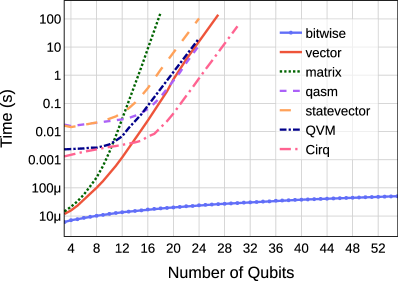
(a) Benchmark for GHZ state preparation.

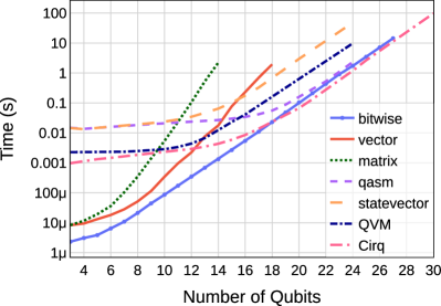
(b) Benchmark for the preparation of an equal superposition state, Equation (14).

Figure 1:

Equal superposition state benchmark.

We now move to a benchmark where no gain is expected for the bitwise representation: the preparation of a state with an equal superposition of all computational basis states, given by

$$\ket{\psi}=\frac{1}{\sqrt{2^{n}}}\sum_{k=0}^{2^{n}-1}\ket{k}.$$ (14)

The circuit used here consists of the application of a Hadamard gate to all qubits, which were initialized in their $\ket{0}$ state. While the number of required gates again scales linearly with the number of qubits, the number of basis states required scales exponentially. As expected, this state preparation suffers from an exponential time scaling, shown in Figure 1b. However, we note that this scaling is comparable to the Cirq simulator, which had the best performance.

Entangled registers benchmark.

The next benchmark is for the preparation of state

$$\ket{\psi}=\frac{1}{\sqrt{2^{n}}}\sum_{k=0}^{2^{n}-1}\ket{k}\otimes\ket{k}.$$ (15)

This can be seen as a bipartite state with each partition containing $n$ qubits. The circuit starts with two registers with $n$ qubits each, all initialized to $\ket{0}$. The circuit described above is then applied to the first register, creating the state

$$\ket{\psi}=\left(\frac{1}{\sqrt{2^{n}}}\sum_{k=0}^{2^{n}-1}\ket{k}\right)\otimes\left(\ket{0}^{\otimes n}\right).$$ (16)

After that, CNOTs are applied between the $i$-th qubit of each register, having the $i$-th qubit in the first register as control and the $i$-th qubit in the second register as target, thus creating the desired state of Equation (15). This is an interesting benchmark as the desired state has features of both previous benchmarks. The first part of the state preparation is precisely the one used above, with an observed exponential scaling, but the second part does not change the size of the Hashmap holding the quantum state. This happens because each basis state is mapped to a unique new one, e.g. $\ket{k}\otimes\ket{0}^{\otimes n}\rightarrow\ket{k}\otimes\ket{k}$.

Figure 2a shows the benchmark results which confirm the exponential scaling of all simulators. However, the bitwise representation displays a much better performance and reduced scaling.

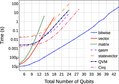
(a) Benchmark for the preparation of entangled registers, Equation (15).

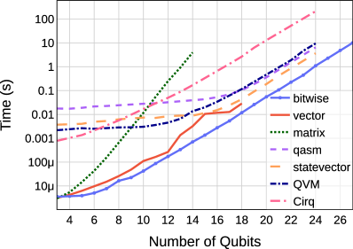
(b) Benchmark for measurement of all qubits for an initial state given by Equation (14).

Figure 2:

Random number measurement

Our last benchmark is designed to test the efficiency of the measurement scheme in the bitwise representation. The circuit first prepares a test state, in this case the equal superposition state of Equation (14), and then measures each qubit, returning the collapsed state, as well an $n$-bit string with the measurement results. In the bitwise representation the measurement scheme is a sequential application of Algorithm 4 to each qubit. Figure 2b shows the time taken for the measurement circuit, determined by the subtraction of the complete run time and the time used to create the state, as displayed in Figure 1b. With the exception of the matrix simulators, all other simulators show similar exponential scalings. However, the bitwise operations show an overhead reduction of more than an order of magnitude when compared to Cirq. We note that an optimization flag used in QVM was turned off in order to clearly determine the measurement time. The measurement algorithm was not optimized to take into account the multiple simultaneous measurements. This could done by, e.g., determining the probabilities of all measurement outcomes in a single loop through the Hashmaps keys and selecting the obtained results form this distribution.

6 Conclusion

We presented the bitwise representation as a powerful tool for quantum circuit simulations. This was implemented in the more general framework of $\mathcal{Q}$System, a quantum circuit simulator for Python that can be used to study and develop quantum algorithms, protocols and error studies. The bitwise representation takes advantage of a Hashmap to store quantum states and gates and bitwise logical and shift operations to speedup simulations. Benchmarking against popular simulators such as Qiskit, Forest SDK and Cirq, we showed that, as predicted from its construction model, this operations show exponential speedups when the simulated state does not require a large number of computational basis states to be fully described. It is also interesting to notice that even in situations where no speedup was expected, an exponential scaling comparable to the other simulators was obtained.

It is important to notice that the exponential gain does not depend on any knowledge of which basis states are required, but only on the fact that the size of this set is not exponentially increasing. Moreover, while the current implementation on $\mathcal{Q}$System  uses the Pauli Z operator to define the computational basis states, other basis states can be considered for problems known to be more efficiently described in other basis sets. One such possibility could be to implement similar bitwise implementations to simulate circuits with states well described by Matrix Product States [39]. It is also interesting to see that entanglement is not directly related to the observed speedups, as the biggest gains where obtained for the generation of the genuinely, maximally entangled GHZ state.

While the current implementation relies on Hashmaps to hold the quantum state, the bitwise representation can also be implemented on other data structure types. This may prove helpful as Hashmaps have a high memory usage. The current version of $\mathcal{Q}$System  was not optimized for memory use.

Detailed documentation for $\mathcal{Q}$System  can be found in Reference [32] and the full numerical simulations are available in Reference [40].

References

References

- [1] Shor P W 1997 SIAM Journal on Computing 26 1484–1509 ISSN 00975397 (Preprint quant-ph/9508027)
- [2] Grover L K 1996 A fast quantum mechanical algorithm for database search Proceedings of the Annual ACM Symposium on Theory of Computing vol Part F129452 (Association for Computing Machinery) pp 212–219 ISBN 0897917855 ISSN 07378017 (Preprint quant-ph/9605043)
- [3] Farhi E, Goldstone J and Gutmann S 2014 (Preprint 1411.4028)
- [4] Peruzzo A, McClean J, Shadbolt P, Yung M H, Zhou X Q, Love P J, Aspuru-Guzik A and O’Brien J L 2014 Nature Communications 5 4213 ISSN 20411723 (Preprint 1304.3061)
- [5] Dallaire-Demers P L and Wilhelm F K 2016 Physical Review A 93 32303 ISSN 24699934 (Preprint 1508.04328)
- [6] Biamonte J, Wittek P, Pancotti N, Rebentrost P, Wiebe N and Lloyd S 2017 Nature 549 195–202 ISSN 14764687 (Preprint 1611.09347)
- [7] Govia L C, Taketani B G, Schuhmacher P K and Wilhelm F K 2017 Quantum Science and Technology 2 15002 ISSN 20589565 (Preprint 1606.08096)
- [8] Taketani B G, Govia L C and Wilhelm F K 2018 Physical Review A 97 52132 ISSN 24699934
- [9] Hempel C, Maier C, Romero J, McClean J, Monz T, Shen H, Jurcevic P, Lanyon B P, Love P, Babbush R, Aspuru-Guzik A, Blatt R and Roos C F 2018 Physical Review X 8 31022 ISSN 21603308 (Preprint %****␣main.bbl␣Line␣50␣****1803.10238)
- [10] Schmit R P, Taketani B G and Wilhelm F K 2020 PLoS ONE 15 e0229382 ISSN 19326203
- [11] Aspuru-Guzik A, Dutoi A D, Love P J and Head-Gordon M 2005 Science 309 1704–1707 ISSN 00368075
- [12] Sieberer L M, Olsacher T, Elben A, Heyl M, Hauke P, Haake F and Zoller P 2019 npj Quantum Information 5 78 ISSN 20566387 (Preprint 1812.05876)
- [13] Moll N, Barkoutsos P, Bishop L S, Chow J M, Cross A, Egger D J, Filipp S, Fuhrer A, Gambetta J M, Ganzhorn M, Kandala A, Mezzacapo A, Müller P, Riess W, Salis G, Smolin J, Tavernelli I and Temme K 2018 Quantum Science and Technology 3 30503 ISSN 20589565 (Preprint 1710.01022)
- [14] Gustafson E, Meurice Y and Unmuth-Yockey J 2019 Physical Review D 99 94503 ISSN 24700029 (Preprint 1901.05944)
- [15] Messinger A, Taketani B G and Wilhelm F K 2019 Physical Review A 99 ISSN 24699934 (Preprint 1810.03446)
- [16] Lamm H, Lawrence S and Yamauchi Y 2019 Physical Review D 100 34518 ISSN 24700029 (Preprint 1903.08807)
- [17] Wang H, Zhuravel A P, Indrajeet S, Taketani B G, Hutchings M D, Hao Y, Rouxinol F, Wilhelm F K, Lahaye M D, Ustinov A V and Plourde B L 2019 Physical Review Applied 11 ISSN 23317019 (Preprint 1812.02579)
- [18] Preskill J 2018 Quantum 2 79 ISSN 2521-327X (Preprint 1801.00862)
- [19] Johansson J R, Nation P D and Nori F 2012 Computer Physics Communications 183 1760–1772 ISSN 00104655 (Preprint 1110.0573)
- [20] Johansson J R, Nation P D and Nori F 2013 Computer Physics Communications 184 1234–1240 ISSN 00104655 (Preprint 1211.6518)
- [21] Smith R S, Curtis M J and Zeng W J 2016 (Preprint 1608.03355)
- [22] Gidney C, Bacon D and The Cirq Developers 2018 quantumlib/Cirq: A python framework for creating, editing, and invoking Noisy Intermediate Scale Quantum (NISQ) circuits. URL https://github.com/quantumlib/Cirq
- [23] Steiger D S, Häner T and Troyer M 2018 Quantum 2 49 ISSN 2521-327X (Preprint 1612.08091)
- [24] Abraham H, Akhalwaya I Y, Aleksandrowicz G, Alexander T, Alexandrowics G, Arbel E, Asfaw A, Azaustre C, Barkoutsos P, Barron G, Bello L, Ben-Haim Y, Bishop L S, Bosch S, Bucher D, CZ, Cabrera F, Calpin P, Capelluto L, Carballo J, Chen C F, Chen A, Chen R, Chow J M, Claus C, Cross A W, Cross A J, Cruz-Benito J, Cryoris, Culver C, Córcoles-Gonzales A D, Dague S, Dartiailh M, Davila A R, Ding D, Dumitrescu E, Dumon K, Duran I, Eendebak P, Egger D, Everitt M, Fernández P M, Frisch A, Fuhrer A, Gacon J, Gadi, Gago B G, Gambetta J M, Garcia L, Garion S, Gawel-Kus, Gil L, Gomez-Mosquera J, de la Puente González S, Greenberg D, Gunnels J A, Haide I, Hamamura I, Havlicek V, Hellmers J, Herok Ł, Horii H, Howington C, Hu W, Hu S, Imai H, Imamichi T, Iten R, Itoko T, Javadi-Abhari A, Jessica, Johns K, Kanazawa N, Karazeev A, Kassebaum P, Krishnan V, Krsulich K, Kus G, LaRose R, Lambert R, Latone J, Lawrence S, Liu P, Mac P B Z R L, Maeng Y, Malyshev A, Marecek J, Marques M, Mathews D, Matsuo A, McClure D T, McGarry C, McKay D, Meesala S, Mezzacapo A, Midha R, Minev Z, Morales R, Murali P, Müggenburg J, Nadlinger D, Nannicini G, Nation P, Naveh Y, Nick-Singstock, Niroula P, Norlen H, O’Riordan L J, Ollitrault P, Oud S, Padilha D, Paik H, Perriello S, Phan A, Pistoia M, Pozas-iKerstjens A, Prutyanov V, Pérez J, Quintiii, Raymond R, Redondo R M C, Reuter M, Rodr’iguez D M, Ryu M, Sandberg M, Sathaye N, Schmitt B, Schnabel C, Scholten T L, Schoute E, Sertage I F, Shi Y, Silva A, Siraichi Y, Sivarajah S, Smolin J A, Soeken M, Steenken D, Stypulkoski M, Takahashi H, Taylor C, Taylour P, Thomas S, Tillet M, Tod M, de la Torre E, Trabing K, Treinish M, TrishaPe, Turner W, Vaknin Y, Valcarce C R, Varchon F, Vogt-Lee D, Vuillot C, Weaver J, Wieczorek R, Wildstrom J A, Wille R, Winston E, Woehr J J, Woerner S, Woo R, Wood C J, Wood R, Wood S, Wootton J, Yeralin D, Yu J, Zdanski L, Zoufalc, Anedumla, Azulehner, Bcamorrison, Drholmie, Fanizzamarco, Kanejess, Klinvill, Merav-aharoni, Ordmoj, Tigerjack, Yangluh and Yotamvakninibm 2019 Qiskit: An Open-source Framework for Quantum Computing
- [25] Jones T, Brown A, Bush I and Benjamin S C 2019 Scientific Reports 9 10736 ISSN 20452322 (Preprint 1802.08032)
- [26] Killoran N, Izaac J, Quesada N, Bergholm V, Amy M and Weedbrook C 2019 Quantum 3 129 ISSN 2521-327X (Preprint 1804.03159)
- [27] Pednault E, Gunnels J A, Nannicini G, Horesh L, Magerlein T, Solomonik E, Draeger E W, Holland E T and Wisnieff R 2017 (Preprint 1710.05867)
- [28] Arute F, Arya K, Babbush R, Bacon D, Bardin J C, Barends R, Biswas R, Boixo S, Brandao F G, Buell D A, Burkett B, Chen Y, Chen Z, Chiaro B, Collins R, Courtney W, Dunsworth A, Farhi E, Foxen B, Fowler A, Gidney C, Giustina M, Graff R, Guerin K, Habegger S, Harrigan M P, Hartmann M J, Ho A, Hoffmann M, Huang T, Humble T S, Isakov S V, Jeffrey E, Jiang Z, Kafri D, Kechedzhi K, Kelly J, Klimov P V, Knysh S, Korotkov A, Kostritsa F, Landhuis D, Lindmark M, Lucero E, Lyakh D, Mandrà S, McClean J R, McEwen M, Megrant A, Mi X, Michielsen K, Mohseni M, Mutus J, Naaman O, Neeley M, Neill C, Niu M Y, Ostby E, Petukhov A, Platt J C, Quintana C, Rieffel E G, Roushan P, Rubin N C, Sank D, Satzinger K J, Smelyanskiy V, Sung K J, Trevithick M D, Vainsencher A, Villalonga B, White T, Yao Z J, Yeh P, Zalcman A, Neven H and Martinis J M 2019 Nature 574 505–510 ISSN 14764687 (Preprint %****␣main.bbl␣Line␣175␣****1911.00577)
- [29] Pednault E, Gunnels J A, Nannicini G, Horesh L and Wisnieff R 2019 (Preprint 1910.09534)
- [30] Nielsen M A, Chuang I and Grover L K 2002 Quantum Computation and Quantum Information vol 70 (Cambridge University Press) ISBN 978-1-139-49548-6
- [31] Gottesman D 1997 Stabilizer Codes and Quantum Error Correction Ph.D. thesis Caltech (Preprint quant-ph/9705052)
- [32] Rosa E C R and Taketani B G 2019 QSystem URL https://gitlab.com/evandro-crr/qsystem
- [33] Beazley D 1996 SWIG: An easy to use tool for integrating scripting languages with C and C++ Proceedings of the 4th conference on USENIX Tcl/Tk (TCLTK’96 vol 4) (USENIX Association) pp 15–15 ISBN 1-880446-78-2
- [34] Coppersmith D 2002 (Preprint quant-ph/0201067)
- [35] Sanderson C and Curtin R 2016 The Journal of Open Source Software 1 26 ISSN 2475-9066
- [36] Sanderson C and Curtin R 2019 Mathematical and Computational Applications 24 70 (Preprint 1811.08768)
- [37] Radhakrishnan S, Kolippakkam D and Mathura V S 2007 Introduction to algorithms (The MIT Press) ISBN 9783540241669
- [38] Luo X, Meyer J J, Wood C J and J G 2019 quantum-benchmarks URL https://github.com/Roger-luo/quantum-benchmarks
- [39] Perez-Garcia D, Verstraete F, Wolf M M and Cirac J I 2007 Quantum Information and Computation 7 401–430 ISSN 15337146 (Preprint quant-ph/0608197)
- [40] Rosa E C R and Taketani B G 2020 qs_benchmark URL https://gitlab.com/evandro-crr/qs_benchmark