Policy iteration for Hamilton-Jacobi-Bellman equations with control constraints

Abstract.

Policy iteration is a widely used technique to solve the Hamilton Jacobi Bellman (HJB) equation, which arises from nonlinear optimal feedback control theory. Its convergence analysis has attracted much attention in the unconstrained case. Here we analyze the case with control constraints both for the HJB equations which arise in deterministic and in stochastic control cases. The linear equations in each iteration step are solved by an implicit upwind scheme. Numerical examples are conducted to solve the HJB equation with control constraints and comparisons are shown with the unconstrained cases.

Keywords: Optimal Feedback Control, $\mathcal{H}_{2}$ control synthesis, Hamilton-Jacobi-Bellman Equations, Policy iteration, Upwind scheme.

AMS classification: 49J20, 49L20, 49N35, 93B52.

1. Introduction

Stabilizability is one of the major objectives in the area of optimal control theory. Since the open loop control depends only on the time and the initial state, so if the initial state is changed, unfortunately control needs to be recomputed again. In many physical situation, we are particularly interested in seeking a control law which depends on the state and which can deal additional external perturbation or model errors. When the dynamical systems is linear with unconstrained control and corresponding cost functional or performance index is quadratic, then the associated closed loop or feedback control law which minimizes the cost functional is obtained by the so called Riccati equation. Now when the dynamics is nonlinear, one popular approach is to linearize the dynamics and obtain the Riccati based controller to apply for the original nonlinear system, see e.g. [33].

If the optimal feedback cannot be obtained by LQR theory, then it can be approached by the verification theorem and the value function, which in turn is a solution of the Hamilton Jacobi Bellman (HJB) equation associated to the optimal control problem, see e.g. [21]. But in most of the situations, it is very difficult to obtain the exact value function and thus one has to resort to iterative techniques. One possible approach utilizes the so called value iteration. Here we are interested in more efficient technique, known as policy iteration. Discrete counterpart of policy iteration is also known as Howards’ algorithm [27], compare also [10]. Policy iteration can be interpreted as a Newton method applied to the HJB equation. Hence, using the policy iteration HJB equation reduces to a sequence of linearized HJB equation, which for historical reasons are called ’generalized HJB equations’. The policy iteration requires as initialization a stabilizing control. If such a control is not available, then one can use discounted path following policy iteration, see e.g. [28]. The focus of the present paper is the analysis of the policy iteration in the presence of control constraints. To the authors’ knowledge, such an analysis is not available in the literature.

Let us next mentions very selectively, some of the literature on the numerical solution of the control-HJB equations. Specific comments for the constraint case, are given further below. Finite difference methods and vanishing viscosity method are developed in the work of Crandall and Lions [17]. Other notable techniques are finite difference methods [16], semi-Lagrangian schemes [4, 19], the finite element method [26], filtered schemes [11], domain decomposition methods [14], and level set methods [36]. For an overview we refer to [20]. Policy iteration algorithms are developed in [32, 37, 8, 9]. If the dynamics are given by a partial differential equation (PDE), then the corresponding HJB equations become infinite dimensional. Applying grid based scheme to convert PDE dynamics to ODE dynamics leads to a high dimensional HJB equation. This phenomenon is known as the curse of dimensionality. In the literature there are different techniques to tackle this situation. Related recent works include, polynomial approximation [28], deep neural technique [31], tensor calculus [18], Taylor series expansions [13] and graph-tree structures [5].

Iteration in policy space for second order HJB PDEs arising in stochastic control is discussed in [40]. Tensor calculus technique is used in [39] where the associated HJB equation becomes linear after using some exponential transformation and scaling factor. For an overview for numerical approximations to stochastic HJB equations, we refer to [30]. To solve the continuous time stochastic control problem by the Markov chain approximation method (MCAM) approach, the diffusion operator is approximated by a finite dimensional Markov decision process, and further solved by the policy iteration algorithm. For the connection between the finite difference method and the MCAM approach for the second order HJB equation, see [12]. Let us next recall contributions for the case with control constraints. Regularity of the value function in the presence of control constraints has been discussed in [24, 25] for linear dynamics and in [15] for nonlinear systems. In [34] non-quadratic penalty functionals were introduced to approximately include control constraints. Later in [1] such functionals were discussed in the context of policy iteration for HJB equations.

Convergence of the policy iteration without constraints has been investigated in earlier work, see in particular [37, 40]. In our work, the control constraints are realized exactly by means of a projection operator. This approach has been used earlier only for numerical purposes in the context of the value iteration, see [23] and [29]. In our work we prove the convergence of the policy iteration with control constraints for both the first and the second order HJB-PDEs. For numerical experiments we use an implicit upwind scheme as proposed in [2].

The rest of the paper is organized as follows. Section $2$ provides a convergence of the policy iteration for the first order HJB equation in the presence of control constraints. Section $3$ establishes corresponding convergence result for the second order HJB equation with control constraints. Numerical tests are presented in Section $4$. Finally in Section $5$ concluding remarks are given.

2. Nonlinear $\mathcal{H}_{2}$ feedback control problem subject to deterministic system

2.1. First order Hamilton-Jacobi-Bellman equation

We consider the following infinite horizon optimal control problem

(2.1) $$\underset{u(\cdot)\in\mathcal{U}}{\min}\;\mathcal{J}(x,u(\cdot)):=\int\limits_{0}^{\infty}\Big{(}\ell(y(t))+\|u(t)\|_{R}^{2}\Big{)}\,dt,$$

subject to the nonlinear deterministic dynamical constraint

(2.2) $$\dot{y}(t)=f(y(t))+g(y)u(t)\,,\quad y(0)=x,$$

where $y(t)=(y_{1}(t),\ldots,y_{d}(t))^{t}\in\mathbb{R}^{d}$ is the state vector, and $u(\cdot)\in\mathcal{U}$ is the control input with $\mathcal{U}=\{u(t):\,\mathbb{R}_{+}\rightarrow U\subset\mathbb{R}^{m}\}$. Further $\ell(y)>0$, for $y\neq 0$, is the state running cost, and $\|u\|_{R}^{2}=u^{t}Ru$, represents the control cost, with $R\in\mathbb{R}^{m\times m},\,R>0$ a positive definite matrix. Throughout we assume that the dynamics $f$ and $g$, as well as $\ell$ are Lipschitz continuous on $\mathbb{R}^{d}$, and that $f(0)=0$ and $\ell(0)=0$. We also require that $g$ is globally bounded on $R^{d}$. This set-up relates to our aim of asymptotic stabilization to the origin by means of the control $u$. We shall concentrate on the case where the initial conditions are chosen from a domain $\Omega\subset\mathbb{R}^{d}$ containing the origin in its interior.

The specificity of this work relates to controls which need to obey constraints $u(t)\in U$, where $U$ is a closed convex set containing $0$ in $\mathbb{R}^{m}$. As a special case we mention bilateral point-wise constraints of the form

(2.3) $$U=\{u\,|\,\alpha\leq u\leq\beta\},$$

where $\alpha=(\alpha_{1},\ldots,\alpha_{m})\in\mathbb{R}^{m}$, $\beta=(\beta_{1},\ldots,\beta_{m})\in\mathbb{R}^{m}$, $\alpha\leq 0,$ $\beta\geq 0$, and the inequalities act coordinate-wise.

The optimal value function associated to (2.1)-(2.2) is given by

$$V(x)=\underset{u(\cdot)\in\mathcal{U}}{\min}\mathcal{J}(x,u(\cdot)),$$

where $x\in\Omega$. Here and throughout the paper we assume that for every $x\in\Omega$ a solution to (2.1) exists. Thus, implicitly we also assume that the existence of a control $u\in L^{2}(0,\infty;\mathbb{R}^{m})$ such that (2.2) admits a solution $y\in W^{1,2}(0,\infty;\mathbb{R}^{d})$. If required by the context, we shall indicate the dependence of $y$ on $x\in\Omega$ or $u\in\mathcal{U}$, by writing $y(\cdot;x)$, respectively $y(\cdot;u)$.

In case $V\in C^{1}(\mathbb{R}^{d})$ it satisfies the Hamilton-Jacobi-Bellman (HJB) equation

(2.4) $$\underset{u\in U}{\inf}\{\nabla V(x)^{t}(f(x)+g(x)u)+\ell(x)+\|u\|_{R}^{2}\}=0\,,\quad V(0)=0\,,$$

with $\nabla V(x)=(\partial_{{x}_{1}}V,\ldots,\partial_{{x}_{d}}V)^{t}$. Otherwise, sufficient conditions which guarantee that $V$ is the unique viscosity solution to (2.4) are well-investigated, see for instance [6, Chapter III].

In the unconstrained case, with $U=\mathbb{R}^{m}$ the value function is always differentiable (see [6, pg. 80]). If $\ell=x^{t}Qx$, with $Q$ a positive definite matrix, and linear control dynamics of the form $f(y)+g(y)u=Ay+Bu$, the value function is differentiable provided that $U$ is nonempty polyhedral (finite horizon) or closed convex set with $0\in int\hskip 2.84544ptU$ (infinite horizon), see [24, 25]. Sufficient conditions for (local) differentiability of the value function associated to finite horizon optimal control problems with nonlinear dynamics and control constraints have been obtained in [15]. For our analysis, we assume that

Assumption 1.

The value function satisfies $V\in C^{1}(\mathbb{R}^{d})$. Moreover it is radially unbounded, i.e. $\lim_{\|x\|\to\infty}V(x)=\infty$.

With Assumption 1 holding, the verification theorem, see eg. [22, Chapter 1] implies that an optimal control in feedback form is given as the minimizer in (2.4) and thus

(2.5) $$u^{*}(x)=\mathcal{P}_{U}\Big{(}-\frac{1}{2}R^{-1}g(x)^{t}\nabla V(x)\Big{)},$$

where $\mathcal{P}_{U}$ is the orthogonal projection in the $R$-weighted inner product on $\mathbb{R}^{m}$ onto $U$, i.e.

$$(R^{-1}g(x)^{t}\nabla V(x)+2u^{*},u-u^{*})_{R}\geq 0\text{ for all }u\in U.$$

Alternatively $u^{*}$ can be expressed as

$$u^{*}(x)=R^{-\frac{1}{2}}\mathcal{P}_{\bar{U}}\Big{(}-\frac{1}{2}R^{-\frac{1}{2}}g(x)^{t}\nabla V(x)\Big{)},$$

where $\mathcal{P}_{\bar{U}}$ is the orthogonal projection in $\mathbb{R}^{m}$, with Euclidean inner product, onto $\bar{U}=R^{\frac{1}{2}}U$. For the particular case of (2.3) we have

$$u^{*}(x)=\mathcal{P}_{U}\Big{(}-\frac{1}{2}R^{-1}g(x)^{t}\nabla V(x)\Big{)}=\min\Big{\{}\beta,\max\{\alpha,-\frac{1}{2}R^{-1}g(x)^{t}\nabla V(x)\}\Big{\}},$$

where the $\max$ and $\min$ operations operate coordinate-wise. It is common practice to refer to the open loop control as in (2.1) and to the closed loop control as in (2.5) by the same letter.

For the unconstrained case the corresponding control law reduces to $u^{*}(x)=-\frac{1}{2}R^{-1}g(x)^{t}\nabla V(x)$. Using the optimal control law $u(x)=\mathcal{P}_{U}\Big{(}-\frac{1}{2}R^{-1}g(x)^{t}\nabla V(x)\Big{)}$ in (2.4), (where we now drop the superscript ^∗) we obtain the equivalent form of the HJB equation as

(2.6) $$\nabla V(x)^{t}\Bigg{(}f(x)+g(x)\mathcal{P}_{U}\Big{(}-\frac{1}{2}R^{-1}g(x)^{t}\nabla V(x)\Big{)}\Bigg{)}+\ell(x)+\left\lVert\mathcal{P}_{U}\Big{(}-\frac{1}{2}R^{-1}g(x)^{t}\nabla V(x)\Big{)}\right\rVert^{2}_{R}=0.$$

We shall require the notion of generalized Hamilton-Jacobi-Bellman (GHJB) equations (see e.g. [37, 7]), given as follows:

(2.7) $$GHJB(V,\nabla V;u):=\nabla V^{t}\Big{(}f+gu\Big{)}+\Big{(}\ell+\left\lVert u\right\rVert^{2}_{R}\Big{)}=0,\qquad V(0)=0,$$

Here $f,g$ and $u$ are considered as functions of $x\in\mathbb{R}^{d}$.

Remark 1.

Concerning the existence of a solution in the unconstrained case to the Zubov type equation (2.7), we refer to [33, Lemma 2.1, Theorem 1.1] where it is shown in the analytic case that if $(\frac{\partial f}{\partial y}(0),g(0))$ is a stabilizable pair, then (2.8) admits a unique locally positive definite solution $V(x)$, which is locally analytic at the origin.

For solving (2.6) we analyse the following iterative scheme, which is referred to as policy iteration or Howards’ algorithm, see e.g. [37, 4, 7, 10], where the case without control constraints is treated. We require the notion of admissible controls, a concept introduced in [32, 7].

Definition 1.

(Admissible Controls). A measurable function $u:\mathbb{R}^{d}\to U\subset\mathbb{R}^{m}$ is called admissible with respect to $\Omega$, denoted by $u\in\mathcal{A}(\Omega)$, if

• $u$ is continuous on $\mathbb{R}^{m}$,

• $u(0)=0$,

• $u$ stabilizes (2.2) on $\Omega$, i.e. $\lim_{t\to\infty}y(t;u)=0,\quad\forall x\in\Omega$.

• $\int\limits_{0}^{\infty}\Big{(}\ell(y(t;u))+\|u(y(t;u))\|_{R}^{2}\Big{)}\,dt<\infty,\quad\forall x\in\Omega$.

Here $y(t;u)$ denotes the solution to (2.2), where $x\in\Omega$, and with control in feedback form $u(t)=u(y(t;u))$. As in (2.1) the value of the cost in (iv) associated to the closed loop control is denoted by $\mathcal{J}(x,u)=\int\limits_{0}^{\infty}(\ell(y(t;u))+\|u(y(t;u))\|_{R}^{2})\,dt$. In general we cannot guarantee that the controlled trajectories $t\to y(t;u(t))$ remain in $\Omega$ for all $t$. For this reason we demand continuity and differentiability properties of $u$ and $V$ on all of $\mathbb{R}^{d}$. Under additional assumptions we could introduce a set $\tilde{\Omega}$ with $\Omega\subsetneq\tilde{\Omega}\subsetneq\mathbb{R}^{d}$ with the property that $\{y(t,u):t\in[0,\infty),u\in\mathcal{A}(\Omega)\}\subset\tilde{\Omega}$ and demanding the regularity properties of $u$ and $V$ on $\tilde{\Omega}$ only. We shall not pursue such a set-up here.

We are now prepared the present the algorithm.

  Input: Let $u^{(0)}:\mathbb{R}^{d}\mapsto U\subset\mathbb{R}^{m}$ be an admissible control law for the dynamics (2.2) and let $\epsilon>0$ be a given tolerance.

  While $\sup_{x\in\Omega}|u^{(i+1)}(x)-u^{(i)}(x)|\geq\epsilon$,  

  Solve for $V^{(i)}\in C^{1}(\mathbb{R}^{d}):$

(2.8) $$\nabla V^{(i)}(x)^{t}\big{(}f(x)+g(x)u^{(i)}(x)\big{)}+\ell(x)+\|u^{(i)}(x)\|^{2}_{R}=0\,\mbox{ with }V^{(i)}(0)=0\,,$$

  Update the Control:

(2.9) $$u^{(i+1)}(x)=\mathcal{P}_{U}\Big{(}-\frac{1}{2}R^{-1}g(x)^{t}\nabla V^{(i)}(x)\Big{)}\,.$$

End

Algorithm 1 Continuous policy iteration algorithm for first order HJB equation

Note that (2.8) can equivalently be expressed as $GHJB(V^{(i)},\nabla V^{(i)};u^{(i)})=0,\,V^{(i)}(0)=0$.

Lemma 1.

Assume that $u(\cdot)$ is an admissible feedback control with respect to $\Omega$. If there exists a function $V(\cdot;u)\in C^{1}(\mathbb{R}^{d})$ satisfying

(2.10) $$GHJB(V,\nabla V;u)=\nabla V(x;u)^{t}(f(x)+g(x)u(x))+\ell(x)+\left\lVert u(x)\right\rVert^{2}_{R}=0,\quad V(0;u)=0,$$

then $V(x;u)=\mathcal{J}(x,u)$ for all $x\in\Omega$. Moreover, the optimal control law $u^{*}(x)$ is admissible on $\mathbb{R}^{d}$, the optimal value function $V(x)$ satisfies $V(x)=\mathcal{J}(x,u^{*})$, and $0<V(x)\leq V(x;u)$.

Proof.

The proof takes advantage, in part, from the verification of an analogous result in the unconstrained, see eg. [37], where a finite horizon problem is treated. Let $x\in\Omega$ be arbitrary and fixed, and choose any $T>0$. Then we have

(2.11) $$V(y(T;u);u)-V(x;u)=\int_{0}^{T}\frac{d}{dt}V(y(t;u))\;dt.$$

Since $\lim_{T\to\infty}y(T;u)=0$ by (iii), and due to V(0;u)=0, we can take the limit $T\to\infty$ in this equation to obtain

$$V(y(\infty;u);u)-V(x;u)=-V(x;u) =\int_{0}^{\infty}\frac{d}{dt}V(y(t;u);u)\;dt$$

(2.12) $$=\int_{0}^{\infty}\nabla V(y;u)^{t}(f(y)+g(y)u(y)))\;dt,$$

where $y=y(t;u)$ on the right hand side of the above equation. Adding both sides of $\mathcal{J}(x,u)=\int_{0}^{\infty}(\ell(y)+\left\lVert u\right\rVert^{2}_{R})\;dt$ to the respective sides of (2.1), we obtain

$$\mathcal{J}(x,u)-V(x;u)=\int_{0}^{\infty}\Big{(}\nabla V(y;u)^{t}(f(y)+g(y)u(y))+\ell(y)+\left\lVert u(y)\right\rVert^{2}_{R}\Big{)}dt,$$

and from (2.10) we conclude that $V(x;u)=\mathcal{J}(x,u)$ for all $x\in\Omega$.

Let us next consider the optimal feedback law $u^{*}(x)$. We need to show that it is admissible in the sense of Definition 1. By Assumption 1 and (2.5) it is continuous on $\mathbb{R}^{d}$. Moreover $V(0)=0$, $V(x)>0$ for all $0\neq x\in\Omega$, thus $\nabla V(0)=0$, and consequently $u^{*}(0)=0$. Here we also use that $0\in U$. Thus (i) and (ii) of Definition 1 are satisfied for $u^{*}$ and (iv) follows from our general assumption that (2.1) has a solution for every $x\in\Omega$. To verify (iii), note that from (2.11), (2.5), and (2.6) we have for every $T>0$

(2.13) $$V(y(T;u^{*}))-V(x)=-\int^{T}_{0}\ell(y(t;u^{*}))+\|u^{*}(y(t;u^{*}))\|_{R}^{2}\;dt<0.$$

Thus $T\to V(y(T;u^{*}))$ is strictly monotonically decreasing, (unless $y(T;u^{*})=0$ for some $T$). Thus $\lim_{T\to\infty}V(y(T;u^{*}))=\epsilon$ for some $\epsilon\geq 0$. If $\lim_{T\to\infty}y(T;u^{*})\neq 0$, then there exists $\epsilon>0$ such that $\epsilon\leq V(y(T;u^{*}))\leq V(x)$ for all $T\geq 0$. Let $S=\{z\in\mathbb{R}^{d}:\epsilon\leq V(z)\leq V(x)\}$. Due to continuity of $V$ the set $S$ is closed. The radial unboundedness assumption on $V$ further implies that $S$ is bounded and thus it is compact. Let us set

$$\dot{V}(x)=\nabla V(x)^{t}(f(x)+g(x)\mathcal{P}_{U}(-\frac{1}{2}R^{-1}g(x)^{t}\nabla V(x)))\text{ for }x\in\mathbb{R}^{d}.$$

Then by (2.6) we have

$$\dot{V}(x)=-\ell(x)-\|{\mathcal{P}_{U}(-\frac{1}{2}R^{-1}g(x)^{t}\nabla V(x))}\|^{2}_{R}<0.$$

By compactness of $S$ we have $\max_{z\in S}\dot{V}(z)=:\zeta<0$. Note that $\{T:y(T;u^{*})\}\subset S$. Hence by (2.13) we find

$$\lim_{T\to\infty}V(y(T;u^{*}))-V(x)\leq\lim_{T\to\infty}\zeta T,$$

which is impossible. Hence $\lim_{T\to\infty}y(T;u^{*})=0$ and $u^{*}\in\mathcal{A}(\Omega)$.

Now we can apply the arguments from the first part of the proof with $u=u^{*}$ and obtain $V(x)=\mathcal{J}(x,u^{*})\leq\mathcal{J}(x,u)=V(x;u)$ for every $u\in\mathcal{A}(\Omega)$. This concludes the proof. ∎

2.2. Convergence of policy iteration

The previous lemma establishes the fact that the value $\mathcal{J}(x,u)$, for a given admissible control $u$, and $x\in\Omega$ can be obtained as the evaluation of the solution of the GHJB equation (2.10). In the following lemma we commence the analysis of the convergence of Algorithm 1.

Proposition 1.

If $u^{(0)}\in\mathcal{A}(\Omega)$, then $u^{(i)}\in\mathcal{A}(\Omega)$ for all $i$. Moreover we have $V(x)\leq V^{(i+1)}(x)\leq V^{(i)}(x)$. Further, $\{V^{(i)}(x)\}$ converges from above pointwise to some $\bar{V}(x)\geq V(x)$ in $\Omega$.

Proof.

We proceed by induction. Given $u^{(0)}\in\mathcal{A}(\Omega)$, we assume that $u^{(i)}\in\mathcal{A}(\Omega)$, and establish that $u^{(i+1)}\in\mathcal{A}(\Omega)$. We shall frequently refer to Lemma 1 with $V^{(i)}:=V(\cdot;u^{i})$ and $V^{(i)}$ as in (2.8). In view of (2.9) $u^{(i+1)}$ is continuous since $g$ is continuous and $V^{(i)}\in C^{1}(\Omega)$. Using Lemma 1 we obtain that $V^{(i)}$ is positive definite. Hence it attains its minimum at the origin, $\nabla V^{(i)}(0)=0$ and consequently $u^{(i+1)}(0)=0$. Thus (i) and (ii) in the definition of admissibility of $u^{(i+1)}$ are established.

Next we take the time-derivative of $t\to V^{(i)}(y(u^{(i+1)})(t)$ where $y(u^{(i+1)})$ is the trajectory corresponding to

$$\dot{y}(t)=f(y(t))+g(y)u^{(i+1)}(y(t))\,,\quad y(0)=x.$$

Let us recall that ${\nabla V^{(i)}(y)}^{t}f(y)=-{\nabla V^{(i)}(y)}^{t}g(y)u^{(i)}(y)-\ell(y)-\left\lVert u^{(i)}(y)\right\rVert^{2}_{R}$, for $y\in\mathbb{R}^{d}$ and set $y^{(i+1)}=y(u^{(i+1)})$. Then we find

(2.14) $$\begin{array}[]{l}\frac{d}{dt}V^{(i)}(y^{(i+1)}(t))={\nabla V^{(i)}(y^{(i+1)})}^{t}(f(y^{(i+1)})+g(y^{(i+1)})u^{(i+1)}(y^{i+1})\\[7.3194pt] =-\ell(y^{(i+1)})\!-\!\left\lVert u^{(i)}(y^{(i+1)})\right\rVert^{2}_{R}+{\nabla V^{(i)}(y^{(i+1)})}^{t}g(y^{(i+1)})\big{(}u^{(i+1)}(y^{(i+1)})-u^{(i)}(y^{(i+1)})\big{)}.\end{array}$$

Throughout the following computation we do not indicate the dependence on $t$ on the right hand side of the equality. Next we need to rearrange the terms on the right hand side of the last expression. For this purpose it will be convenient to introduce $z=\frac{1}{2}R^{-1}g(y^{(i+1)})^{t}{\nabla V^{(i)}(y^{(i+1)})}$ and observe that $u^{(i+1)}=\mathcal{P}_{U}(-z)$. We can express the above equality as

$$\frac{d}{dt}V^{(i)}(y^{(i+1)}(t)) =-\ell(y^{(i+1)})-\left\lVert u^{(i)}(y^{(i+1)})\right\rVert^{2}_{R}+2z^{t}R\mathcal{P}_{U}(-z)-2z^{t}R\,u^{(i)}(y^{(i+1)})$$

$$=-\ell(y^{(i+1)})-\|\mathcal{P}_{U}(-z)\|_{R}^{2}-\|u^{(i)}(y^{(i+1)})-\mathcal{P}_{U}(-z)\|_{R}^{2}$$

$$\quad+2(z+\mathcal{P}_{U}(-z))^{t}R(\mathcal{P}_{U}(-z)-u^{(i)}(y^{(i+1)})).$$

Since $u^{(i)}(y^{(i+1)})\in U$ we obtain $(z+\mathcal{P}_{U}(-z))^{t}R(\mathcal{P}_{U}(-z)-u^{(i)}(y^{(i+1)}))\leq 0$, and thus

(2.15) $$\frac{d}{dt}V^{(i)}(y^{(i+1)}(t))\leq-\ell(y^{(i+1)})-\|u^{(i+1)}(y^{(i+1)})\|^{2}_{R}-\|u^{(i+1)}(y^{(i+1)})-u^{(i)}(y^{(i+1)})\|^{2}_{R}.$$

Hence $t\to V^{(i)}(y^{(i+1)}(t))$ is strictly monotonically decreasing. As mentioned above, $V^{i}$ is positive definite. With the arguments as in the last part of the proof of Lemma 1 it follows that $\lim_{t\to\infty}y^{(i+1)}(t)=\lim_{t\to\infty}y(t;u^{(i+1)})=0$. Finally (2.15) implies that $0\leq\int_{0}^{\infty}\Big{(}\ell(y(t;u^{(i+1)}))+\|u^{(i+1)}(y^{(i+1)})(t)\|_{R}^{2}\Big{)}\,dt\leq V^{(i)}(x)$. Since $x\in\Omega$ was chosen arbitrarily it follows that $u^{(i+1)}$ defined in (2.9) is admissible. Lemma 1 further implies that $V^{(i+1)}(x)\geq V(x)$ on $\Omega$.

Since for each $x\in\Omega$ the trajectory $y^{(i+1)}$ corresponding to $u^{(i+1)}$ and satisfying

(2.16) $$\dot{y} =\Big{(}f(y)+g(y)u^{(i+1)}\Big{)},\quad y(0)=x,$$

is asymptotically stable, the difference between $V^{(i+1)}(x)$ and $V^{(i)}(x)$ can be obtained as

$$V^{(i+1)}(x)-V^{(i)}(x) =\int_{0}^{\infty}\Bigg{(}\Big{(}\nabla V^{(i)}(y^{(i+1)})^{t}(f+gu^{(i+1)})\Big{)}-\Big{(}{\nabla V^{(i+1)}}^{t}(f+gu^{(i+1)})\Big{)}\Bigg{)}\;dt,$$

where $f$ and $g$ are evaluated at $y^{(i+1)}$. Utilizing the generalized HJB equation (2.8), we get ${\nabla V^{(i)}(y^{(i+1)})}^{t}(f+gu^{(i+1)})={\nabla V^{(i)}(y^{(i+1)})}^{t}g(u^{(i+1)}-u^{(i)})-(\ell+\left\lVert u^{(i)}\right\rVert^{2}_{R})$ and ${\nabla V^{(i+1)}(y^{(i+1)})}^{t}(f+gu^{(i+1)})=-(\ell+\left\lVert u^{(i+1)}\right\rVert^{2}_{R})$. This leads to

$$V^{(i+1)}(x)-V^{(i)}(x)=\int^{\infty}_{0}\big{(}\|u^{(i+1)}\|^{2}_{R}-\|u^{(i)}\|^{2}_{R}+{\nabla V^{(i)}(y^{(i+1)})}^{t}g(u^{(i+1)}-u^{(i)})\big{)}dt.$$

The last two terms in the above integrand appeared in (2.14) and were estimated in the subsequent steps. We can reuse this estimate and obtain

$$V^{(i+1)}(x)-V^{(i)}(x)\leq-\int^{\infty}_{0}\|u^{(i+1)}-u^{(i)}\|^{2}_{R}\,dt\leq 0.$$

Hence, $\{V^{(i)}\}$ is a monotonically decreasing sequence which is bounded below by the optimal value function $V$, see Lemma 1. Since $\{V^{(i)}\}$ is a monotonically decreasing sequence and bounded below by $V$, it converges pointwise to some $\bar{V}\geq V$. ∎

To show convergence of $u^{(i)}$ to $\bar{u}:=\mathcal{P}_{U}(-\frac{1}{2}R^{-1}g(x)^{t}\nabla\bar{V}(x))$, additional assumptions are needed. This is considered in the following proposition. In the literature, for the unconstrained case, one can find the statement that, based on Dini’s theorem, the monotonically convergent sequence $\{V^{(i)}\}$ converges uniformly to $\bar{V}$, if $\Omega$ is compact. This, however, only holds true, once it is argued that $\bar{V}$ is continuous. For the following it will be useful to recall that $C^{m}(\bar{\Omega})$, $m\in\mathbb{N}_{0}$, consists of all functions $\phi\in C^{m}(\Omega)$ such that $D^{\alpha}\phi$ is bounded and uniformly continuous on $\Omega$ for all multi-index $\alpha$ with $0\leq\alpha\leq m$, see e.g. [3, pg. 10].

Proposition 2.

If $\Omega$ is bounded, and further $\{V^{(i)}\}\subset C^{1}(\Omega)$ satisfy (2.8), $\bar{V}\in C^{1}(\Omega)\cap C(\bar{\Omega})$, and $\{\nabla V^{(i)}\}$ is equicontinuous in $\Omega$, then $\{\nabla V^{(i)}\}$ converges pointwise to $\nabla\bar{V}$ in $\Omega$, and $\bar{V}$ satisfies the HJB equation (2.6) for all $x\in\Omega$ with $\bar{V}(x)=V(x)$ for all $x\in\Omega$.

Proof.

Let $x\in\Omega$ and $\epsilon>0$ be arbitrary. Denote by $e_{k}$ the $k$-th unit vectors, $k=1,\ldots,d,$ and choose $\delta_{1}>0$ such that $S_{x}=\{x+h:|h|\leq\delta_{1}\}\;\subset\Omega$. By continuity of $\nabla\bar{V}$ and equicontinuity of $\nabla V^{(i)}$ in $\Omega$, there exists $\delta\in(0,\delta_{1})$ such

(2.17) $$\|\nabla\bar{V}(x)-\nabla\bar{V}(x+h)\|<\frac{\epsilon}{3}\quad\text{and}\quad\|\nabla V^{(i)}(x)-\nabla V^{(i)}(x+h)\|<\frac{\epsilon}{3},$$

with for all $h$ with $|h|\leq\delta$, $k=\{1,\ldots,d\}$, $i=1,2,\ldots$.

By assumption $\Omega$ is bounded and thus $\bar{\Omega}$ is compact. Hence by Dini’s theorem $V^{(i)}$ converges to $\bar{V}$ uniformly on $\bar{\Omega}$. Here we use the assumption that $\bar{V}\in C(\bar{\Omega})$. We can now choose $\bar{i}>0$ such that

(2.18) $$|\bar{V}(y)-V^{(i)}(y)|\leq\frac{\epsilon\delta}{6}\quad\forall\,y\in\Omega,\quad\text{and }\forall\,i\geq\bar{i}.$$

We have

$$\partial_{x_{k}}\bar{V}(x)-\partial_{x_{k}}V^{(i)}(x)$$

$$=\Big{(}\partial_{x_{k}}\bar{V}(x)-\frac{1}{\delta}\big{(}\bar{V}(x+e_{k}\delta)-\bar{V}(x)\big{)}\Big{)}+\frac{1}{\delta}\Big{(}\big{(}\bar{V}(x+e_{k}\delta)-\bar{V}(x)\big{)}-\big{(}V^{(i)}(x+e_{k}\delta)-V^{(i)}(x)\big{)}\Big{)}$$

$$\qquad+\Big{(}\frac{1}{\delta}\big{(}V^{(i)}(x+e_{k}\delta)-V^{(i)}(x)\big{)}-\partial_{x_{k}}V^{(i)}(x)\Big{)}=:I_{1}+I_{2}+I_{3}.$$

We estimate $I_{1}$ and $I_{3}$ by using (2.17) as

$$|I_{1}|=\frac{1}{\delta}|\int_{0}^{1}\Big{(}\partial_{x_{k}}\bar{V}(x)-\partial_{x_{k}}\bar{V}(x+e_{k}\sigma\delta)\Big{)}\delta\;d\sigma|\leq\frac{\epsilon}{3},$$

and

$$|I_{3}|=\frac{1}{\delta}|\int_{0}^{1}\Big{(}\partial_{x_{k}}V^{(i)}(x+e_{k}\sigma\delta)-\partial_{x_{k}}V^{(i)}(x)\Big{)}\delta\;d\sigma|\leq\frac{\epsilon}{3}.$$

We estimate $I_{2}$ by using (2.18)

$$|I_{2}|\leq\frac{\epsilon}{3},$$

and combining with the estimates for $I_{1}$ and $I_{3}$, we obtain

(2.19) $$\|\nabla\bar{V}(x)-\nabla V^{(i)}(x)\|\leq\epsilon\sqrt{d}.$$

Since $x\in\Omega$ was arbitrary this implies that

$$\nabla V^{i}\to\nabla\bar{V}\quad\text{pointwise in}\quad\Omega.$$

It then follows from (2.9) that

$$\lim_{i\to\infty}\mathcal{P}_{U}\Big{(}-\frac{1}{2}R^{-1}g(x)^{t}\nabla V^{(i)}(x)\Big{)}=\lim_{i\to\infty}u^{(i+1)}(x)=\mathcal{P}_{U}\Big{(}-\frac{1}{2}R^{-1}g(x)^{t}\nabla\bar{V}(x)\Big{)}=:\bar{u}(x),\hskip 2.84544pt\text{in}\hskip 2.84544pt\Omega,$$

and by (2.8)

$$\nabla\bar{V}(x)^{t}(f(x)+g\bar{u})+\ell(x)+\left\lVert\bar{u}\right\rVert^{2}_{R}=0,\quad\forall x\in\Omega.$$

For uniqueness of value function $\bar{V}=V$, we refer to [22, pg. 86] and [6, Chapter III]. ∎

While the assumptions of Proposition 2 describe a sufficient conditions for pointwise convergence of $\nabla V^{(i)}$, is appears to be a challenging open issue to check them in practice.

3. Nonlinear $\mathcal{H}_{2}$ control subject to stochastic system

3.1. Second order Hamilton-Jacobi-Bellman equation

Here we consider the stochastic infinite horizon optimal control problem

(3.1) $$\underset{u(\cdot)\in\mathcal{U}}{\min}\;\mathcal{J}(x,u(\cdot)):=\mathbb{E}\int\limits_{0}^{\infty}\Big{(}\ell(y(t))+\left\lVert u(t)\right\rVert^{2}_{R}\Big{)}\,dt,$$

subject to the nonlinear stochastic dynamical constraint

(3.2) $$dy(t) =\Big{(}f(y(t))+g(y)u(t)\Big{)}dt+g_{1}(y)\hskip 2.84544ptdW\,,\quad y(0)=x\in\mathbb{R}^{d},$$

where $y(t)\in\mathbb{R}^{d}$ is the state vector, $W(t)\in\mathbb{R}^{k}$ is a standard multi-dimensional separable Wiener process defined on a complete probability space, and the control input $u(\cdot)\in\mathcal{U}$ is an adapted process with respect to a natural filter. The functions $f,\,g,$ and $g_{1}$ are assumed to be Lipschitz continuous on $\mathbb{R}^{d}$, and satisfy $f(0)=0$, $g(0)=0$ and $g_{1}(0)=0$. For details about existence and uniqueness for (3.2), we refer to e.g. [35, Chapter 2]. As in the previous section $\Omega$ denotes a domain in $\mathbb{R}^{d}$ containing the origin.

The value function $V(x)=\underset{u(\cdot)\in U}{\inf}\mathcal{J}(x,u(\cdot))$ is assumed to be $C^{2}$- smooth over $\mathbb{R}^{d}$. Then the HJB equation corresponding to (3.1) and (3.2) is of the form

(3.3) $$\underset{u\in U}{\min}\Big{\{}\nabla V(x)^{t}(f(x)+g(x)u)+\frac{1}{2}Tr[g_{1}(x)^{t}\frac{\partial^{2}V(x)}{\partial x^{2}}g_{1}(x)]+\Big{(}\ell(x)+\left\lVert u\right\rVert^{2}_{R}\Big{)}\Big{\}}=0\,,\quad V(0)=0\,.$$

From the verification theorem [22, Theorem 3.1], the explicit minimizer $u^{*}$ of (3.3) is given by

$$u^{*}(x) =\underset{u\in U}{argmin}\Big{\{}\nabla V(x)^{t}(f(x)+gu)+\frac{1}{2}Tr[g_{1}(x)^{t}\frac{\partial^{2}V(x)}{\partial x^{2}}g_{1}(x)]+\Big{(}\ell(x)+\left\lVert u\right\rVert^{2}_{R}\Big{)}\Big{\}}$$

(3.4) $$=\mathcal{P}_{U}\Big{(}-\frac{1}{2}R^{-1}g(x)^{t}\nabla V(x)\Big{)}\,,$$

where the projection $\mathcal{P}_{U}$ is defined as in (2.5). The infinitesimal differential generator of the stochastic system (3.2) for the optimal pair $(u,V)$ (dropping the superscript *) is denoted by

$$\mathcal{L}_{u}V(x)=\nabla V(x)^{t}\Big{(}f(x)+g(x)u(x)\Big{)}+\frac{1}{2}Tr[g_{1}(x)^{t}\frac{\partial^{2}V(x)}{\partial x^{2}}g_{1}(x)].$$

Using the optimal control law (3.1) in (3.3), we obtain an equivalent form of the HJB equation

$$\nabla V(x)^{t} \Bigg{(}f(x)+g(x)\mathcal{P}_{U}\Big{(}-\frac{1}{2}R^{-1}g(x)^{t}\nabla V(x)\Big{)}\Bigg{)}+\ell(x)$$

(3.5) $$+\left\lVert\mathcal{P}_{U}\Big{(}-\frac{1}{2}R^{-1}g(x)^{t}\nabla V(x)\Big{)}\right\rVert^{2}_{R}+\frac{1}{2}Tr[g_{1}(x)^{t}\frac{\partial^{2}V(x)}{\partial x^{2}}g_{1}(x)]=0\,.$$

For the unconstrained control, the above HJB equation becomes

(3.6) $$\nabla V(x)^{t}f(x)-\frac{1}{4}\nabla V(x)^{t}g(x)R^{-1}g(x)^{t}\nabla V(x)+\frac{1}{2}Tr[g_{1}(x)^{t}\frac{\partial^{2}V(x)}{\partial x^{2}}g_{1}(x)]+\ell(x)=0\,.$$

The associated generalized second order GHJB equation is of the form

(3.7) $$GHJB(V,\nabla V,\nabla^{2}V;u) =0,\qquad V(0)=0,\text{where}$$

$$GHJB(V,\nabla V,\nabla^{2}V;u) :=\nabla V^{t}\Big{(}f+gu\Big{)}+\frac{1}{2}Tr[g_{1}^{t}\nabla^{2}Vg_{1}]+\Big{(}\ell+\left\lVert u\right\rVert^{2}_{R}\Big{)}.$$

We next define the admissible feedback controls with respect to stochastic set up.

Definition 2.

(Admissible Controls). A control $u$ is defined to be admissible with respect to (3.1), denoted by $u\in\mathcal{A}(\Omega)$ if

• $u$ is continuous on $\mathbb{R}^{m}$,

• $u(0)=0$,

• $u$ stabilizes (3.2) on $\Omega$ stochastically, i.e. $P(\lim_{t\to\infty}y(t;u)=0)=1,\quad\forall\ x\in\Omega$ i.e. when $\mathbb{E}(\lim_{t\to\infty}y(t;u))=0$.

• $\mathbb{E}\int\limits_{0}^{\infty}\Big{(}\ell(y(t;u))+\|u(y(t;u))\|_{R}^{2}\Big{)}\,dt<\infty,\quad\forall\;x\in\Omega$.

In Algorithm 2, the policy iteration for the second order HJB equation is documented, see [40].

Let $u^{(0)}$ be an initial stabilizing control law in the stability region $\Omega$ for system (3.2).

  For $i=0:\infty$ 

  While $\sup_{x\in\Omega}|u^{(i+1)}(x)-u^{(i)}(x)|\geq\text{tolerance}$,  

  Solve for $V^{(i)}$:

(3.8) $$\mathcal{L}_{u^{(i)}(x)}V^{(i)}(x)+\ell(x)+ \left\lVert u^{(i)}(x)\right\rVert^{2}_{R}=0\,,\,V^{(i)}(0)=0,$$

End

  Update the Control:

(3.9) $$u^{(i+1)}(x)=\mathcal{P}_{U}\Big{(}-\frac{1}{2}R^{-1}g^{t}\nabla V^{(i)}(x))\Big{)}\,.$$

  End

Algorithm 2 Policy iteration algorithm for the second order HJB equation

Lemma 2.

Assume that $u(\cdot)$ is an admissible feedback control in $\Omega$. If there exist a function $V(\cdot;u)\in C^{2}(\mathbb{R}^{d})$ satisfying

(3.10) $$GHJB(V,\nabla V,\nabla^{2}V;u)=\mathcal{L}_{u}V(x)+\ell(x)+\left\lVert u(x)\right\rVert^{2}_{R}=0,\quad V(0;u)=0,$$

then $V(x;u)$ is the value function of the system (3.2) and $V(x;u)=J(x,u)$ $\forall x\in\Omega$. Moreover, the optimal control law $u^{*}(x)$ is admissible and the optimal value function $V(x;u^{*})$, if it exists and is radial unbounded, satisfies $V(x;u^{*})=\mathcal{J}(x,u^{*})$, and $0<V(x;u^{*})\leq V(x;u)$.

Proof.

By Itô’s formula [35, Theorem 6.4] for any $T>0$

$$V(y(T);u)-V(x;u)$$

$$=\int_{0}^{T}dV(y(t;u);u)$$

$$=\int_{0}^{T}\Big{(}\nabla V(y;u))^{t}(f(y)+g(y)u(y))+Tr[\frac{1}{2}g_{1}(y)^{t}\frac{\partial^{2}V(y;u))}{\partial y^{2}}g_{1}(y)]\Big{)}\;dt$$

$$\qquad+\int_{0}^{T}\nabla V(y;u))^{t}g_{1}(y)\;dW.$$

Taking the expectation with limit as $T\to\infty$ on both sides, the above equation becomes

(3.11) $$\mathbb{E}\;(\lim_{T\to\infty}V(y(T);u))-V(x;u) =-V(x;u)=\mathbb{E}\int_{0}^{\infty}\mathcal{L}_{u(y)}V(y)\;dt,$$

where $\mathbb{E}\int_{0}^{t}\nabla V(y;u)^{t}g_{1}(y)\;dW=0$ for each time $t\geq 0$, with $\mathbb{E}(\lim_{T\to\infty}V(y(T);u))=0$. Adding $\mathcal{J}(x,u)=\mathbb{E}\int_{0}^{\infty}(\ell(y)+\left\lVert u(y)\right\rVert^{2}_{R})\;dt$ to (3.11), we obtain

$$\mathcal{J}(x,u)-V(x;u) =\mathbb{E}\int_{0}^{\infty}\Big{(}\mathcal{L}_{u(y)}V(y)+\ell(y)+\left\lVert u(y)\right\rVert^{2}_{R}\Big{)}dt.$$

Hence $V(x;u)=\mathcal{J}(x,u)$ for all $x\in\Omega$.
Concerning the admissibility of $u^{*}$, properties $(i)$, $(ii)$ and $(iv)$ in Definition 2, can be shown similarly as in Lemma 1. Since the stochastic Lyapunov functional $V$ is radially unbounded by assumption, and its differential generator $\mathcal{L}_{u^{*}}V$ satisfies $\mathcal{L}_{u^{*}}V(x)=-(\ell(x)+\left\lVert u^{*}\right\rVert^{2}_{R})$ as well as

$$\mathbb{E}V(y(T;u^{*}))-V(x)=-\mathbb{E}\int_{0}^{T}\Big{(}\ell(y)+\left\lVert u^{*}\right\rVert^{2}_{R}\Big{)}\;dt,\,\,\text{for each}\;T>0,$$

one can follow the standard argument given in Theorem [35, Theorem 2.3-2.4] to obtain
$P(\lim_{t\to\infty}y(t;u^{*})=0)=1,\quad\forall\ x\in\Omega$ and hence $u^{*}\in\mathcal{A}(\Omega)$. ∎

3.2. Convergence of policy iteration

Here we turn to the convergence analysis of the iterates $V^{(i)}$.

Proposition 3.

If $u^{(0)}\in\mathcal{A}(\Omega)$, then $u^{(i)}\in\mathcal{A}(\Omega)$ for all $i$. Further we have $V(x)\leq V^{(i+1)}(x)\leq V^{(i)}(x)$, where $V$ satisfies the HJB equation (3.1). Moreover $\{V^{(i)}\}$ converges pointwise to some $\bar{V}\geq V$ in $\Omega$.

Proof.

First we show that if $u^{(i)}\in\mathcal{A}(\Omega)$, then $u^{(i+1)}\in\mathcal{A}(\Omega)$. As $g$ is continuous and $V^{(i)}\in C^{1}(\Omega)$, we have $u^{(i+1)}$ is continuous by (3.9). Since $V^{(i)}$ is positive definite, it attains a minimum at the origin and hence $\nabla V^{(i)}(0)=0$ and consequently $u^{(i+1)}(0)=0$. The infinitesimal generator $\mathcal{L}_{u}V(y)$ evaluated along the trajectories generated by $u^{(i+1)}$ becomes

$$\mathcal{L}_{u}V^{(i)}(y;u^{(i+1)}) ={\nabla V^{(i)}}^{t}(f(y)+g(y)u^{(i+1)})+\frac{1}{2}Tr[g_{1}(y)^{t}\frac{\partial^{2}V^{(i)}(y)}{\partial y^{2}}g_{1}(y)]$$

(3.12) $$=-\ell(y)-\left\lVert u^{(i)}\right\rVert^{2}_{R}+{\nabla V^{(i)}}^{t}g(u^{(i+1)}-u^{(i)}),$$

where ${\nabla V^{(i)}}^{t}f+\frac{1}{2}Tr[g_{1}^{t}\frac{\partial^{2}V^{(i)}}{\partial y^{2}}g_{1}]=-{\nabla V^{(i)}}^{t}gu^{(i)}-\ell(y)-\left\lVert u^{(i)}\right\rVert^{2}_{R}$.
Now we can calculate $\mathcal{L}_{u}V^{(i)}(y;u^{(i+1)})$ as in Proposition 1 to show that $\mathcal{L}_{u}V^{(i)}(y;u^{(i+1)})<0$. By the stochastic Lyapunov theorem [35, Theorem 2.4], it follows that $P(\lim_{t\to\infty}y(t;u^{(i+1)})=0)=1$, i.e. $\mathbb{E}(\lim_{t\to\infty}y(t;u^{i+1}))=0$. Since $\mathcal{L}_{u}V^{(i)}(y;u^{(i+1)})<0$, we find

(3.13) $$\mathbb{E}\int_{0}^{T}\Big{(}\ell(y(t;u^{(i+1)}))+\left\lVert u^{(i+1)}\right\rVert^{2}_{R}\Big{)}dt<V^{(i)}(x)\quad\forall\;T>0,$$

and thus $u^{(i+1)}$ is admissible.
Using that $dy=\Big{(}f(y)+g(y)u^{(i)}\Big{)}dt+g_{1}(y)\hskip 2.84544ptdW$ is asymptotically stable for all $i$, by Itô’s formula along the trajectory

(3.14) $$dy =\Big{(}f(y)+g(y)u^{(i+1)}\Big{)}dt+g_{1}(y)\hskip 2.84544ptdW,$$

the difference $V^{(i+1)}(x)-V^{(i)}(x)$ can be obtained as

$$V^{(i+1)}(x;u^{(i+1)})-V^{(i)}(x;u^{(i+1)})$$

$$=\mathbb{E}\int_{0}^{\infty}\Bigg{(}\Big{(}{\nabla V^{(i)}}^{t}(f+gu^{(i+1)})+\frac{1}{2}Tr[g_{1}^{t}\frac{\partial^{2}V^{(i)}}{\partial y^{2}}g_{1}]\Big{)}$$

$$\qquad-\Big{(}{\nabla V^{(i+1)}}^{t}(f+gu^{(i+1)})+\frac{1}{2}Tr[g_{1}^{t}\frac{\partial^{2}V^{(i+1)}}{\partial y^{2}}g_{1}]\Big{)}\Bigg{)}dt=:\mathbb{E}\int_{0}^{\infty}(A-B)\;dt.$$

Using the generalized HJB equation (3.8) for two consecutive iterations $(i)$ and $(i+1)$, we have $\frac{1}{2}Tr[g_{1}^{t}\frac{\partial^{2}V^{(i)}}{\partial y^{2}}g_{1}]=-{\nabla V^{(i)}}^{t}(f+gu^{(i)})-(\ell+\left\lVert u^{(i)}\right\rVert^{2}_{R})$ and ${\nabla V^{(i+1)}}^{t}(f+gu^{(i+1)})+\frac{1}{2}Tr[g_{1}^{t}\frac{\partial^{2}V^{(i+1)}}{\partial y^{2}}g_{1}]=-(\ell+\left\lVert u^{(i+1)}\right\rVert^{2}_{R})$ respectively. Applying $u^{(i+1)}(y)=\mathcal{P}\Big{(}-\frac{1}{2}R^{-1}g^{t}\nabla V^{(i)}(y))\Big{)}$, we obtain finally

$$A-B=-\Big{(}\left\lVert u^{(i)}\right\rVert^{2}_{R}-\left\lVert u^{(i+1)}\right\rVert^{2}_{R}\Big{)}+{\nabla V^{(i)}}^{t}g(u^{(i+1)}-u^{(i)}),$$

where $A-B$ can be calculated as in Proposition 1 to obtain $V^{(i+1)}(x)\leq V^{(i)}(x)$. Further, $V(x)\leq V^{(i+1)}(x)$. Therefore, $\{V^{(i)}\}$ converges pointwise to some $\bar{V}$. ∎

Now, in addition if $\Omega$ is compact and $\bar{V}$ is continuous, then by Dini’s theorem $\{V^{(i)}\}$ converges uniformly to $\bar{V}$.

Proposition 4.

Let $\Omega$ be a bounded domain. If $\{V^{(i)}\}\in C^{2}(\Omega)$ satisfy (3.8), $\bar{V}\in C^{2}(\Omega)\cap C^{1}(\bar{\Omega})$, and $\{\nabla^{m}V^{(i)}\}$ is equicontinuous, then $\{\nabla^{m}V^{(i)}\}$ converges pointwise to $\nabla^{m}\bar{V}$ in $\Omega$, for $m=1$, $2$, and $\bar{V}$ satisfies the HJB equation (3.1) with $\bar{V}=V$.

Proof.

From Proposition 2, it follows that $\{\nabla V^{(i)}\}$ converges pointwise to $\nabla\bar{V}$ in $\Omega$ and $\bar{u}(x)=\mathcal{P}_{U}\Big{(}-\frac{1}{2}R^{-1}g(x)^{t}\nabla\bar{V}(x)\Big{)}$. Pointwise convergence of $\{\nabla^{2}V^{(i)}\}$ to $\nabla^{2}\bar{V}$ can be argued as for the first derivatives which was done in the proof of Proposition 2. We can now pass to the limit $i\to\infty$ in (3.8) to obtain that $\bar{V}$ satisfies the HJB equation (3.1). Concerning the uniqueness of the value function $\bar{V}=V$, we refer to e.g. [22, pg. 247]. ∎

4. Numerical examples

Here we conduct numerical experiments to demonstrate the feasibility of the policy iteration in the presence of constraints and to compare the solutions between constrained and unconstrained formulations. To describe a setup which is independent of a stabilizing feedback we also introduce a discount factor $\lambda>0$. Unless specified otherwise we choose $\lambda=0.05$, and we also give results with $\lambda=0$.

Test 1: One dimensional linear equation.

Consider the following minimization problem

$$\underset{u(\cdot)}{\min}\;\mathcal{J}(x_{0},u(\cdot))=\int_{0}^{\infty}e^{-\lambda t}\Big{(}\left\lVert x\right\rVert^{2}+\left\lVert u(x)\right\rVert^{2}_{R}\Big{)}dt$$

subject to the following deterministic dynamics with control constraint

(4.1) $$\dot{x}(t)=0.5x(t)+u;\quad-1\leq u\leq 1,\quad x(0)=x_{0};$$

and

$$\underset{u(\cdot)}{\min}\;\mathcal{J}(x_{0},u(\cdot))=\mathbb{E}\int_{0}^{\infty}e^{-\lambda t}\Big{(}\left\lVert x\right\rVert^{2}+\left\lVert u(x)\right\rVert^{2}_{R}\Big{)}dt$$

subject to the following stochastic system with control constraint

(4.2) $$dx(t)=(0.5x(t)+u)\hskip 2.84544ptdt+0.005\hskip 2.84544ptdW;\quad-1\leq u\leq 1,\quad x(0)=x_{0},$$

where $\lambda>0$ is the discount factor. We solve the GHJB equation (3.8) combining an implicit method and with an upwind scheme over $\Omega=(-2,2)$ as follows

$$-\frac{(V^{n}_{i}-V^{(n-1)}_{i})}{dt} +\lambda V^{n}_{i}+\nabla V^{n}_{iupwind}(f(x_{i})+gu^{n}_{i})$$

(4.3) $$+\frac{1}{2}g_{1}^{t}(x_{i})D^{2}V^{n}_{i}g_{1}(x_{i})+x_{i}^{2}+\left\lVert u^{n}_{i}\right\rVert^{2}_{R}=0,$$

where the superscript $n$ stands for the iteration loop, the subscript $i$ stands for the mesh point numbering in the state space ($V_{i}\approx V(x_{i})$ for $i=1,\cdots,I\hskip 2.84544pt(\text{total number of grid points})$), $dt$ is the time step, $\Delta x=x_{i+1}-x_{i}$ is the distance between equi-spaced grid points, and $D^{2}V^{n}_{i}=(V^{n}_{i+1}-2V^{n}_{i}+V^{n}_{i-1})/\Delta x^{2}$ is the approximation of the second order derivative of the value function. To solve the first order HJB (2.8), we take $g_{1}=0$ in (4).
For the upwind scheme, we take forward difference $\nabla V_{i,F}=\frac{V_{i+1}-V_{i}}{\Delta x}$ whenever the drift of the state variable $S_{i,F}=f(x_{i})+g(x_{i})u_{i,F}>0$, and backward difference $\nabla V_{i,B}=\frac{V_{i}-V_{i-1}}{\Delta x}$ if the drift $S_{i,B}=f(x_{i})+g(x_{i})u_{i,B}<0$, and $D\bar{V}_{i}=-2R\bar{u}_{i}$ with $\bar{u}_{i}=-f(x_{i})/g(x_{i})$ for $S_{i,F}\leq 0\leq S_{i,B}$. Hence,

$$\nabla V^{n}_{iupwind}=\nabla V^{n}_{i,F}\mbox{1{1}}_{S_{i,F}>0}+\nabla V^{n}_{i,B}\mbox{1{1}}_{S_{i,B}<0}+D\bar{V}^{n}_{i}\mbox{1{1}}_{S_{i,F}\leq 0\leq S_{i,B}},$$

where 11 is the characteristic function. The updated control policy for $(n+1)$ iteration becomes

$$u^{n+1}_{i}=\mathcal{P}_{U=[-1,1]}(-\frac{1}{2}R^{-1}g(x_{i})^{t}\nabla V^{n}_{iupwind}).$$

Note that since we solve the HJB backward in time, it is necessary to construct the upwind scheme as above which is in a reverse compared to the form an upwind scheme for dynamics forward in time. For more details about upwind schemes for HJB, see [2] including its appendix.

We choose, $R=0.1$, $dt=2$, $I=400$ and two different initial conditions $x_{0}=-1.8$ and $x_{0}=1$. Figure 1(i) depicts the value functions in the unconstrained and the constrained case. As expected they are convex. Outside $[-1,1]$ the two value functions differ significantly. In the constrained case it tends to infinity at $\pm 2$ indicating that for such initial conditions the constrained control cannot stabilize anymore. Figure 1(ii), shows the evolution of the states under the effect of the control as shown in 1(iv). In the transient phase, the decay rate for the constrained control system is slower than in the unconstrained case, which is the expected behavior. The temporal behavior of the running cost of $\left\lVert y(t)\right\rVert$ is documented in Figure 1(iii). It is clear that the uncontrolled solution diverges whereas $\left\lVert y(t)\right\rVert^{2}$ tends to zero for the cases with control, both for constrained and unconstrained controls. The pointwise error for the HJB equation (2.6) is documented in Figure 1(v). Similar behavior is achieved for the stochastic dynamics. It is observed from Figure 2(i) that even with the small intensity of noise ($g_{1}=0.005$), we can see the Brownian motion of the state cost for the controlled system. Figure 2(ii) plots that error for the value function of the increasing iteration count.

We have also solved this problem with $\lambda=0$. For this purpose we initialized the algorithm with the solution of the discounted problem with $\lambda=0.05$. If the $dt$ was further reduced, then the algorithm converged. Moreover, the value functionals with $\lambda=0.05$ and $\lambda=0$ are visually indistinguishable.

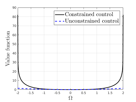
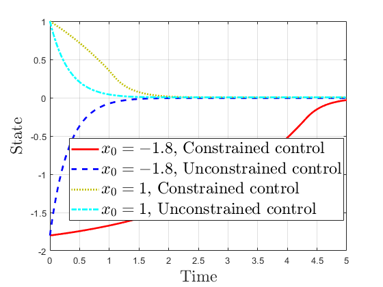
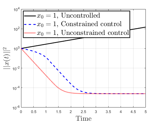
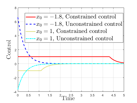
(i) (ii) (iii) (iv) (v)

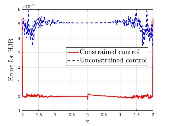
Figure 1. Test 1: Deterministic case. i) Value function, ii) State, iii) State cost $\left\lVert x(t)\right\rVert^{2}$, iv) Control, v) Residue for HJB with discount factor .

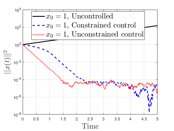
(i) (ii)

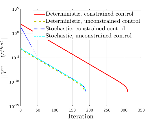
Figure 2. Test 1: Stochastic case. i) State cost $\left\lVert x(t)\right\rVert^{2}$, ii) $||V^{(i)}-V^{Final}||$ for both cases.

The next example focuses on the exclusion of discount factor once we have proper initialization, which is obtained through solving HJB equation with a discount factor.

4.1. Test 2: One dimensional nonlinear equation.

We consider the following infinite horizon problem

$$\underset{u(\cdot)}{\min}\;\mathcal{J}(x_{0},u(\cdot))=\int_{0}^{\infty}\Big{(}\left\lVert x\right\rVert^{2}+\left\lVert u(x)\right\rVert^{2}_{R}\Big{)}dt$$

subject to the following dynamics with control constraint

(4.4) $$\dot{x}(t)=x(t)-x^{3}(t)+u;\quad-1\leq u\leq 1,\quad x(0)=x_{0}.$$

Here $\Omega=(-2,2)$, $dt=0.001$, $R=0.1$, $I=400$. To obtain a proper initialization $(u^{(0)},V^{(0)})$, we solve (4) with discount factor $\lambda=0.05$. Now we can solve (2.8) with the HJB initialization using the aforementioned upwind scheme.

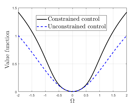
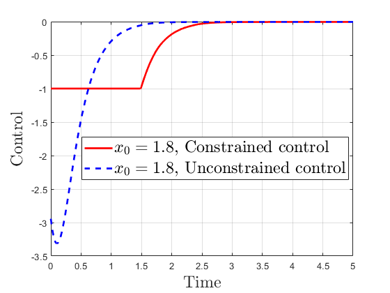
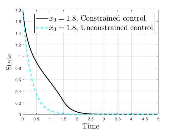
(i) (ii) (iii) (iv)

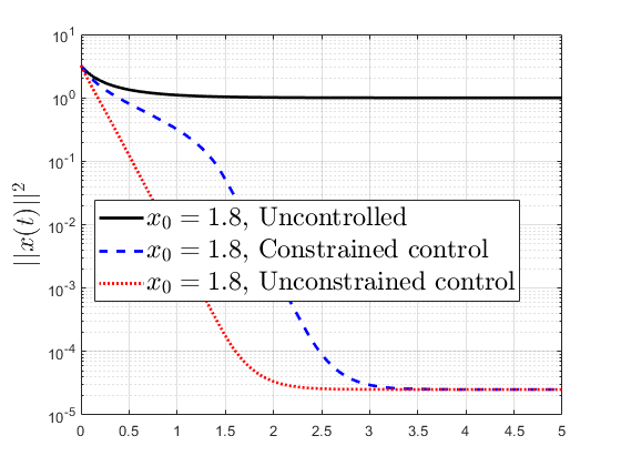
Figure 3. Test 2: Deterministic case. i) Value function, ii) Control, iii) State, iv) State cost.

Behaviors of the value function, state, control and state cost both for the constrained and unconstrained control systems are documented in Figures 3(i)-(iv) with a observation of faster decay rate for trajectories in the unconstrained cases.

4.2. Test 3: Three dimensional linear system

Consider the minimization problem

(4.5) $$\underset{u(\cdot)}{\min}\;\mathcal{J}(u(\cdot),(x_{0},y_{0},z_{0}))=\int_{0}^{\infty}e^{-\lambda t}\Big{(}\left\lVert x\right\rVert^{2}+\left\lVert y\right\rVert^{2}+\left\lVert z\right\rVert^{2}+\left\lVert u_{1}\right\rVert^{2}_{R}+\left\lVert u_{2}\right\rVert^{2}_{R}\Big{)}dt$$

subject to the following 3D linear control system

(4.6) $$\frac{dx}{dt} =\sigma(y-x);\quad x(0)=x_{0},$$

(4.7) $$\frac{dy}{dt} =x\rho-y+u_{1};\quad-1\leq u_{1}\leq 1,\quad y(0)=y_{0},$$

(4.8) $$\frac{dz}{dt} =-\beta z+u_{2};\quad-1\leq u_{2}\leq 1,\quad z(0)=z_{0},$$

with $\sigma=10$, $\rho=1.1$, and $\beta=8/3$. System (4.6)-(4.8) arises from linearization of the Lorenz system at (0,0,0). For $\rho>1$, the equilibrium solution $(0,0,0)$ is unstable [38, Chapter 1].

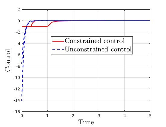
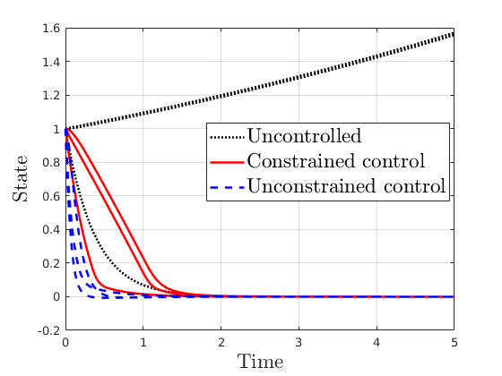
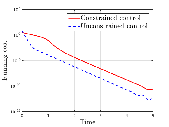
(i) (ii) (iii) (iv)

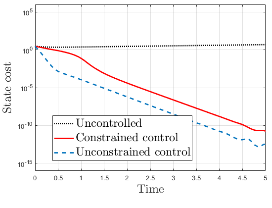
Figure 4. Test 3: Deterministic case, 3D Linear, $R=0.01$,Time step $dt=10$, Initial condition $[x_{0},y_{0},z_{0}]=[1,1,1]$. i) Control, ii) State, iii) Running cost $(\left\lVert x(t)\right\rVert^{2}+\left\lVert y(t)\right\rVert^{2}+\left\lVert z(t)\right\rVert^{2}+\left\lVert u_{1}(t)\right\rVert^{2}_{R})+\left\lVert u_{2}(t)\right\rVert^{2}_{R})$, iv) State cost $\left\lVert x(t)\right\rVert^{2}+\left\lVert y(t)\right\rVert^{2}+\left\lVert z(t)\right\rVert^{2}$ .

Figure 4 (i) depicts the unconstrained and the constrained controls, where one component of the control constraint is active up to $t=0.5$, and the other one up to $t=1$. The first two components of the state of the uncontrolled solution diverge, while the third one converges, see the dotted curves in 4(ii). For the unconstrained HJB control the state tends to zero with a faster decay rate than for the constrained one. See again Figure 4 (ii). Figures 4(iii)-(iv) document the running and state costs, respectively.
We next turn to the stochastic version of problem (4.5)-(4.8) with noise of intensity .05 added to the second and third components.

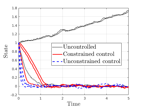
(i) (ii)

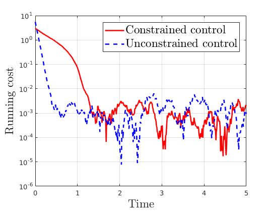
Figure 5. Test 3: Stochastic case, 3D Linear system, $R=0.01$, Time step $dt=10$, Initial condition $[x_{0},y_{0},z_{0}]=[1,1,1]$. i) State, ii) Running cost $(\left\lVert x(t)\right\rVert^{2}+\left\lVert y(t)\right\rVert^{2}+\left\lVert z(t)\right\rVert^{2}+\left\lVert u_{1}(t)\right\rVert^{2}_{R}+\left\lVert u_{2}(t)\right\rVert^{2}_{R})$.

For the stochastic system the constrained and unconstrained states tend to zero with some oscillations, see Figure 5

Test 4: Lorenz system.

For the third test, we choose the Lorenz system which appears in weather prediction, for example. This is a nonlinear three dimensional system, with control appearing in the second equation,

(4.9) $$\frac{dx}{dt} =\sigma(y-x);\quad x(0)=x_{0},$$

(4.10) $$\frac{dy}{dt} =x(\rho-z)-y+u;\quad-1\leq u\leq 1,\quad y(0)=y_{0},$$

(4.11) $$\frac{dz}{dt} =xy-\beta z;\quad z(0)=z_{0},$$

where the three parameters $\sigma>1$, $\rho>0$ and $\beta>0$ have physical interpretation. For more details see e.g. [38]. When $u=0$ in (4.10), we obtain the original uncontrolled Lorenz system. The Lorenz system has 3 steady state solution namely $C0=(0,0,0)$, $C^{+}=\Big{(}\sqrt{\beta(\rho-1)},\sqrt{\beta(\rho-1)},\rho-1\Big{)}$ and $C^{-}=\Big{(}-\sqrt{\beta(\rho-1)},-\sqrt{\beta(\rho-1)},\rho-1\Big{)}$. For $\rho<1$, all steady state solutions are stable. For $\rho>1$, $C0$ is always unstable and $C^{\pm}$ are stable only for $\sigma>\beta+1$ and $1<\rho<\rho^{*}=\frac{\sigma(\sigma+\beta+3)}{(\sigma-\beta-1)}$. At $\rho=\rho^{*}$, $C^{\pm}$ becomes unstable. Here, we take $\sigma=10$, $\beta=8/3$ and $\rho=2$ so that $C0=(0,0,0)$ is an unstable equilibrium. We solve the HJB equation over $\Omega=(-2,2)^{3}$ with $dt=0.1$, and $R=0.01$.

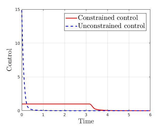
(i) (ii)

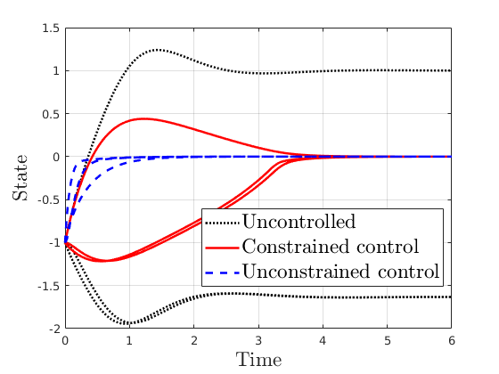
Figure 6. Test 4: Deterministic case, Lorenz system, $R=0.01$, Initial condition $[x_{0},y_{0},z_{0}]=[-1,-1,-1]$. i) Control, ii) State.

From Figure 6(i), it can be observed that the unconstrained HJB control quickly tends to zero whereas the constrained control is active up to $t\sim 3$ and then converges to zero. Figure 6(ii) shows that in absence of control, the state does not tend to the origin but rather to a stable equilibrium. With HJB-constrained or unconstrained control synthesis, the controlled state tends to the origin, with a faster decay rate for the unconstrained control compared to the constrained one.

Similar numerical results were also obtained in the stochastic case.

Concluding remarks

We investigated convergence of the policy iteration technique for the stationary HJB equations which arise from the deterministic and stochastic control of dynamical systems in the presence of control constraints. The control constraints are realized as hard constraints by a projection operator rather than by approximation by means of a penalty technique, for example. Numerical examples illustrate the feasibility of the approach and provide a comparison of the behavior of the closed loop controls in the presence of control constraints and without them. The algorithmic realization is based on an upwind scheme.

References

- [1] M. Abu-Khalaf and F. L. Lewis, Nearly optimal control laws for nonlinear systems with saturating actuators using a neural network HJB approach, Automatica J. IFAC, 41(5)(2005) 779-791.
- [2] Y. Achdou, J. Han, J.-M. Lasry, P.-L. Lions and B. Moll,.Income and wealth distribution in macroeconomics: A continuous-time approach, National Bureau of Economic Research, 2017.
- [3] R. A. Adams and J. J. F. Fournier, Sobolev spaces, Elsevier/Academic Press, Amsterdam, 2003.
- [4] A. Alla, M. Falcone and D. Kalise, An efficient policy iteration algorithm for dynamic programming equations, SIAM J. Sci. Comput., 37(1)(2015) 181-200.
- [5] A. Alla, M. Falcone and L. Saluzzi. An efficient DP algorithm on a tree-structure for finite horizon optimal control problems, SIAM J. Sci. Comput., 41 (2019), 2384–2406.
- [6] M. Bardi and I. Capuzzo-Dolcetta, Optimal control and viscosity solutions of Hamilton-Jacobi-Bellman equations, Birkhäuser Boston, 1997.
- [7] R. W. Beard, G. N. Saridis, and J. T. Wen, Galerkin approximation of the Generalized Hamilton-Jacobi-Bellman equation, Automatica 33(12)(1997) 2159-2177.
- [8] R. W. Beard, G. n. Saridis, and J. T. Wen. Approximate solutions to the Time-Invariant Hamilton-Jacobi-Bellman equation, J. Optim. Theory Appl. 96(3)(1998) 589–626.
- [9] R. W. Beard and T. W. Mclain. Successive Galerkin approximation algorithms for nonlinear optimal and robust control Internat. J. Control 71(5)(1998) 717–743.
- [10] O. Bokanowski, S. Maroso and H. Zidani, Some Properties of Howards’ Algorithm, SIAM J. Numer. Anal. 47(4)(2009), 3001-3026.
- [11] O. Bokanowski, M. Falcone and S. Sahu. An efficient filtered scheme for some first order time-dependent Hamilton-Jacobi equations, SIAM J. Sci. Comput. 38(1) (2016), 171–195.
- [12] J. F. Bonnans, and H. Zidani. Consistency of generalized finite difference schemes for the stochastic HJB equation, SIAM J.Numer. Anal. 41(3)(2003), 1008–1021.
- [13] T. Breiten, K. Kunisch and L. Pfeiffer. Taylor expansions of the value function associated with a bilinear optimal control problem, Ann. I. H. Poincare-AN, In Press, 2019.
- [14] S. Cacace, E. Cristiani, M. Falcone and A. Picarelli. A patchy dynamic programming scheme for a class of Hamilton-Jacobi-Bellman equations, SIAM J. Sci. Comput. 34(5)(2012), 2625–2649.
- [15] P. Cannarsa, and H. Frankowska, Local regularity of the value function in optimal control, Systems Control Lett., 62(9)(2013), 791–794.
- [16] I. Capuzzo-Dolcetta and H. Ishii. Approximate solutions of the Bellman equation of deterministic control theory, Appl. Math. Optim. 11(2)(1984), 161–181.
- [17] M.G. Crandall and P.L. Lions. Two approximations of solutions of Hamilton-Jacobi equations, Math. Comp. 43(167)(1984), 1–19.
- [18] S. Dolgov, D. Kalise and K. Kunisch. Tensor Decompositions for High-dimensional Hamilton-Jacobi-Bellman Equations, arXiv:1908.01533, 2019.
- [19] M. Falcone, and R. Ferretti. Semi-Lagrangian approximation schemes for linear and Hamilton-Jacobi equations, Society for Industrial and Applied Mathematics (SIAM), Philadelphia, 2014.
- [20] M. Falcone, and R. Ferretti. Numerical methods for Hamilton-Jacobi type equations, Handb. Numer. Anal., Elsevier/North-Holland, Amsterdam,17 2016, 603–626.
- [21] W. H. Fleming, and R. W. Rishel. Deterministic and stochastic optimal control, Springer Science & Business Media, 2012.
- [22] W. H. Fleming, and H. M. Soner, Controlled Markov processes and viscosity solutions, Springer Science & Business Media, Philadelphia, 2006.
- [23] J. Garcke and A. Kröner. Suboptimal feedback control of PDEs by solving HJB equations on adaptive sparse grids, J. Sci. Comput., 43 (2017),1–28.
- [24] R. Goebel, Convex optimal control problems with smooth Hamiltonians, SIAM J. Control Optim., 43(5)(2005), 1787–1811.
- [25] R. Goebel and M. Subbotin, Continuous time linear quadratic regulator with control constraints via convex duality, IEEE transactions on automatic control, 52(5)(2007), 886–892.
- [26] R. Gonzalez and E. Rofman. On deterministic control problems: an approximation procedure for the optimal cost. I. The stationary problem, SIAM J. Control Optim. 23(2)(1985), 242–266.
- [27] R. Howard. Dynamic Programming and Markov Processes, The M.I.T. Press, 1960.
- [28] D. Kalise and K. Kunisch. Polynomial approximation of high-dimensional Hamilton-Jacobi-Bellman equations and applications to feedback control of semilinear parabolic PDEs, SIAM J. Sci. Comput. 40(2)(2018), 629–652.
- [29] A. Kröner, K. Kunisch and H. Zidani. Optimal feedback control of undamped wave equations by solving a HJB equation, ESAIM: COCV, EDP Sciences, 21 (2)(2014), 442–464.
- [30] H. J. Kushner and P. Dupuis. Numerical methods for stochastic control problems in continuous time,Springer-Verlag, New York (2001), xii+475.
- [31] K. Kunisch and D. Walter. Semiglobal optimal feedback stabilization of autonomous systems via deep neural network approximation,, arXiv:2002.08625v1.
- [32] R. J. Leake and R.-W. Liu, Construction of Suboptimal Control Sequences, SIAM J. Control 5(1) (1967), 54–63.
- [33] D. L. Lukes, Optimal regulation of nonlinear dynamical systems, SIAM J. Control 7(1) (1969), 75–100.
- [34] S. E. Lyshevski, Optimal control of nonlinear continuous-time systems: design of bounded controllers via generalized nonquadratic functionals, Proceedings of the 1998 American Control Conference. ACC (IEEE Cat. No. 98CH36207) 1(1998), 205–209.
- [35] X. Mao, Stochastic differential equations and applications, Elsevier, 2007.
- [36] S. Osher and R. Fedkiw. Level set methods and dynamic implicit surfaces, Applied Mathematical Sciences, Springer-Verlag, New York, 2003.
- [37] G. N. Saridis and C. S. G. Lee, An approximation theory of optimal control for trainable manipulators, IEEE Trans. Systems Man Cybernet, 9(3)(1979), 152–159.
- [38] C. Sparrow, The Lorenz equations: bifurcations, chaos, and strange attractors, Springer-Verlag, New York-Berlin, 1982.
- [39] E. Stefansson and Y.P. Leong. Sequential Alternating Least Squares for Solving High Dimensional Linear Hamilton-Jacobi-Bellman Equations, Proc. of IEEE/RSJ International Conference on Intelligent Robots and Systems (IROS), doi: 10.1109/IROS.2016.7759553, 2016.
- [40] F.Y. Wang and G. N. Saridis, On successive approximation of optimal control of stochastic dynamic systems, Modeling uncertainty, Internat. Ser. Oper. Res. Management Sci., Kluwer Acad. Publ., Boston, MA 46(2002), 333–358.
Acknowledgments
The authors gratefully acknowledge support by the ERC advanced grant 668998 (OCLOC) under the EU’s H2020 research program.