Adaptive sampling recovery of functions with higher mixed regularity
Abstract.
We tensorize the Faber spline system from [14] to prove sequence space isomorphisms for multivariate function spaces with higher mixed regularity. The respective basis coefficients are local linear combinations of discrete function values similar as for the classical Faber Schauder system. This allows for a sparse representation of the function using a truncated series expansion by only storing discrete (finite) set of function values. The set of nodes where the function values are taken depends on the respective function in a non-linear way. Indeed, if we choose the basis functions adaptively it requires significantly less function values to represent the initial function up to accuracy (say in ) compared to hyperbolic cross projections. In addition, due to the higher regularity of the Faber splines we overcome the (mixed) smoothness restriction and benefit from higher mixed regularity of the function. As a byproduct we present the solution of Problem 3.13 in Triebel’s monograph [46] for the multivariate setting.
1. Introduction
This paper is a continuation of the research that was started in [14], where we constructed a higher order Faber spline basis for the representation of univariate functions from Besov-Lizorkin-Triebel spaces. Compared to wavelet isomorphisms, the coefficient functionals in a Faber spline series expansion are given by a (local) linear combination of discrete function values. In the monographs [45, 46] Triebel used tensor products of the classical Faber-Schauder basis to obtain characterization for bivariate functions. Due to the limited regularity of the hat functions one is not able to benefit from higher smoothness of the respective functions. This leads to a saturation rate for the approximation error. Here we present the corresponding modifications for the multivariate situation to resolve functions with higher mixed Sobolev-Besov regularity. The characterizations are used to sparsely represent a multivariate function by a truncated tensorized Faber spline series. As already observed by Byrenheid in [2] one needs to store significantly less discrete information of the function compared to a hyperbolic cross projection. In fact, to benefit from a non-linear (adaptive) approximation framework we also need to establish characterizations in the quasi-Banach setting. It is well-known (see for instance [23, 15, 36, 17, 18, 19]) that Besov spaces with mixed smoothness , where , serve as nonlinear approximation spaces in with respect to a hyperbolic wavelet dictionary since the spaces are isomorphic to if .
In our paper [14] we study this problem for the univariate situation. We construct a higher order Faber spline basis that allows to get sampling discretizations of Besov function spaces with higher smoothness , and (see Subsection 2.1 for the definition of this basis). The main tool for the construction of higher order Faber splines are the celebrated Chui-Wang wavelets [4]. They serve as the initial point. We apply a “lifting procedure” to the dual Chui-Wang wavelet via a certain integral operator similar as the Faber-Schauder system evolves from integrating the Haar system. With this technique we are able to generate Faber splines of arbitrary high (but limited) smoothness. Although the new basis functions are supported on the real line they are very well localized (exponentially decaying) and the main parts are concentrated on a segment. Note also that for the periodic case very well time-localized (polynomial decay) basis functions were constructed in [24] and [13] for one- and two-dimensional cases. The corresponding characterization of Besov spaces (for the univariate case so far) was obtained in [12].
The sampling characterization of mixed Besov spaces via Faber-Schauder coefficients for dimension has been established in [2]. It is known that coefficients in a series expansion with respect to the tensor product Faber-Schauder basis are represented via second order mixed difference
where we put for and where the latter denotes the second order difference operator which is applied to the -th variable of the function .
The interesting question was if this extends to a higher order framework. This question is answered in this paper. Indeed, if we tensorize the Faber splines from [14] we obtain a linear combination of -th order mixed differences ()
where and is the -th order tensorized -spline (see Section 2 for details) and , where
In the case of approximation by linear sampling algorithms such as for example Smolyak sparse grid operators the set of samples is fixed in advance for the whole class of functions. In this paper we consider adaptive sampling approximation where the set of sample points is chosen for each particular function differently. Namely, we work with the quantity of best -term approximation with respect to this new Faber spline basis. A detailed overview on the history of this subject with regard to different dictionaries is given in [11, Chapt. 10]. We mention here only some papers of Hansen and Sickel [17], [18], [19], D. Dũng [5, 6], Temlyakov [40, 41], V. Romanyuk [30], [31] and Bazarkhanov [1], where the authors considered wavelet type dictionaries. Best -term trigonometric approximation was studied by Temlyakov [44], [43], A. Romanyuk [25], [26], [27], [28], A. Romanyuk and V. Romanyuk [29], Stasyuk [38], [39] and others. Probably closest to us are the papers D. Dũng [7, 9], where the univariate and isotropic framework is considered. Here we consider classes of multivariate functions with mixed smoothness.
We study best -term approximation with respect to the tensorized Faber spline basis constructed in this paper. The main advantage over classical wavelet dictionaries is the fact that the aggregate of best -term approximation is constructed by using only finitely many discrete function values rather than wavelet inner products. The following order estimates are obtained below for function space embedding on a compact . In the so-called case of “small smoothness” we obtain
for and smoothness , whereas in the case of “large smoothness” we find
Note that in case of wavelet type dictionaries and there is a slight improvement in the power of the , namely . These results complement the corresponding results for the Faber-Schauder system, see [2]. Similarly to the Faber-Schauder case the estimates for best -term approximation are realized by a so-called level-wise greedy algorithm that uses coefficients. Due to the construction the number of function values that have to be stored scales similarly.
Outline. This paper has the following structure. In Subsection 2.1 we give the definition of the 1D higher order Faber spline basis that was constructed in [14]. In Subsections 2.2 and 2.3 we define the corresponding basis for the multivariate setting and prove uniform convergence in . In Section 3 we prove the sampling characterization for Besov-Triebel-Lizorkin spaces of mixed smoothness. The main theorem is formulated in Subsection 3.4. In Section 2 we prove the sampling characterization of Besov-Triebel-Lizorkin spaces of mixed smoothness. The main theorem is formulated in Subsection 2.4. In Subsection 2.1 we give definition of 1D higher order Faber spline basis that was constructed in [14]. In Section 4 we consider best -term approximation of Besov-Triebel-Lizorkin spaces of with respect to the higher order Faber spline basis. The main results are presented in Subsections 4.1 and 4.2. The short Subsection 4.3 refers to the constructiveness of the algorithm we use. Finally, definitions of functions spaces and some auxiliary results from harmonic analysis are put to the Appendix A. Examples of the construction of higher order Faber splines for 1D are presented in Appendix B.
Notation. As usual , and are reserved for natural, integer and real numbers. Then let , , and . With letter we indicate dimension of spaces , , and etc. By symbols , we denote elements from vector spaces , , . means the following vector and by we denote a scaling product of two vectors and , i.e. . By we mean . For we denote by the number . For two non negative quantities and we write if there exists a positive constant that does not depend on one of the parameters known from the context such that . We write if and . Let be the space of continuous functions on with the usual supremum norm, be the space of compactly supported continuous functions on . By , as usual we denote the space of Lebesgue measurable functions with the finite norm
2. A higher order tensorized Faber spline basis
In this section we present construction of multivariate higher order Faber splines and prove sampling discretization of Besov and Lizorkin-Triebel spaces of functions with mixed smoothness.
First we give definition of this new basis for the univariate case. The main ideas of the construction for 1D are presented in [14] and further we give only necessary definitions.
2.1. Definition of univariate basis functions
Let , , be the -th order B-spline with knots at defined by
where . Let further and . It is well-known that the system
constitutes a multiresolution analysis of . In [4] it was also proved that there is a compactly supported wavelet that generates the wavelet spaces , usually defined as , represented by the formula
It means that . It is clear that and .
By we denote the dual wavelet of , and by dual of . In [14] we prove an explicit representation for .
Theorem 2.1.
Further we define the cardinal spline function
| (2.1) |
with precisely given exponentially decaying coefficients (see [3] for details). By using the -th order biorthogonal Chui-Wang wavelets and Theorem 2.1 we define the following -th order Faber spline basis for as
| (2.2) |
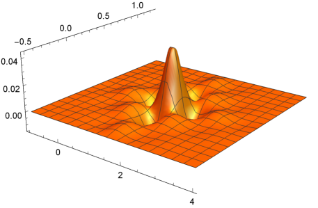
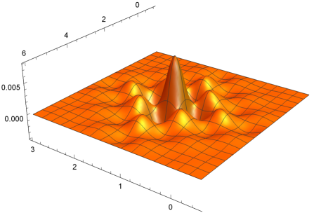
and . Plotted examples of tensorized versions of these basis functions and are given in Figures 2 and 3. For comparison the Faber-Schauder basis function is presented on Figure 1.
We would also like to mention a related univariate construction in the papers [52, 51]. For further details in this regard see [14, Remark 3.6].

2.2. Construction of multivariate basis functions
For the following series converges uniformly
where the coefficients are defined as follows and for
where by we denote a -th order difference of a function with step at the point (see Appendix A.3 for a definition).
Now let a function . Recall that for , , . For we define a set and let , where
We fixed variables and consider the expansion with respect to a variable
Further we expand functions and with respect to a variable . Proceeding in this way for each variable we obtain the following pointwise expansion
| (2.3) |
where basis functions are defined as follows
and coefficients
where and is -th order mixed difference operator acting in the directions contained in (see Appendix A.3 for definition). Further we will use the following notation for the sequence of coefficients , .
2.3. Uniform convergence in the space
Further we show that series (2.3) converges uniformly. First we give some necessary definitions. The univariate cardinal spline function is defined by (2.1). Then for dimension ,
or we can also write
where and . It is clear that for . Further we define the fundamental spline interpolating operator as
and its scaled version , , as
with the following interpolating property for .
Let be a univariate function defined as
| (2.4) |
By we denote the space of multivariate functions of the form
where is defined by (2.4).
Further we state two lemmas.
Lemma 2.2.
Every can be reproduced by the fundamental spline interpolating operator , i.e.
Proof.
The proof is similar to the one-dimensional case (see Lemma 3.2 in [14]). We use the fact that for . ∎
Using the expansion (2.3) we define the operator
Lemma 2.3.
Every can be reproduced by the operator , i.e.
Proof.
The proof follows from the fact for (see Lemma 3.1 [14]) and tensor structure of functions from the space . ∎
As a consequence from this two lemmas we get the following
Lemma 2.4.
For every function we have .
Proof.
Let and . Since according to Lemma 2.2 we have that . On the other hand, since , , according to definition of we get that . ∎
Lemma 2.5.
For each
| (2.5) |
where the constant depends only on .
Proof.
For we have
Since is compactly supported then the sum is finite and depends only on . Since coefficients decay exponentially the sum is also finite and depends only on . Taking this into account we get (2.5). ∎
Theorem 2.6.
For a function , we have that
| (2.6) |
Proof.
By we denote a univariate quasi-interpolation operator (see [10] for details)
where the set is finite and the functional is defined by using finite number of function values. We define the operator for as
Since for 1D the basis functions are defined by
where is defined for as
and , it is clear that are supported on the segment and . We denote a segment
For the multivariate case we will have
where , where are given in Theorem 2.1 and (2.1). To be more precise, if if and if . The function is supported on the cube .
3. Sampling isomorphisms in mixed smoothness spaces
The main goal of this subsection is to prove sequence space isomorphisms with respect to the tensorized Faber spline basis.
Theorem 3.1.
-
(i)
Let , and for and . Then every compactly supported can be represented by the series (2.3), which is convergent unconditionally in the space for every . If we have unconditional convergence in the space . Moreover, the following norms are equivalent
-
(ii)
Let , , and for and . Then every compactly supported can be represented by the series (2.3), which is convergent unconditionally in the space for every . If we have unconditional convergence in the space . Moreover, the following norms are equivalent
Remark 3.2.
For the one-dimensional setting these results were obtained in [14]. The case corresponds to the classical Faber-Schauder basis and the corresponding characterization for was obtained in [45] and for this result was extended in [2]. Note again that our results complement results from [45] and [2], but do not include them.
Remark 3.3.
We would also like to mention about sharpness of the restrictions for the smoothness parameter in Theorem 3.1. First we consider B-case. Lower restriction is natural and assures the embedding in the space of continuous functions. It looks like the upper bound is also sharp because for and .
Now we make some comments about F-case. Note that by using interpolation technique similar to Theorem 4.16 [2] for the -case the range of the smoothness parameter can be extended to . In the recent preprint [37] it was proved that Chui-Wang wavelets constitute an unconditional basis in only if (so far for univariate case only). It is an extension of the corresponding results for Haar wavelets [35] for wavelets of higher regularity. We can say that our new basis functions are in some sense -lifted Chui-Wang wavelets. Therefore the following restriction for smoothness parameter is probably also sharp.
Remark 3.4.
In his papers [7]-[10] D. Dũng offers a different approach to sampling characterization of Besov spaces of mixed smoothness with higher regularity. The main difference with respect to our construction is that D. Dũng considers “frame-type” system while the system is the “basis-type” system in the sense that it is linearly independent. Further we also prove unconditional convergence of this system in Besov-Triebel-Lizorkin spaces.


First we prove some auxiliary statements. We apply some known technique that was also used in [2], [20], [32] and [14].
The following lemma is a multivariate analog of Lemma A.11 from [14]. We formulate it without a proof.
Lemma 3.5.
Let , and . Then for the local means with finitely many vanishing moments of order the following estimates hold
| (3.1) |
and
| (3.2) |
where if , if . The set is the cross product of sets such that .
Proposition 3.6.
-
Let and .
-
(i)
For , , and the inequality
(3.3) holds.
-
(ii)
For , , and the inequality
(3.4) holds.
Proof.
We use the following pointwise representation of (formula (A.1))
| (3.5) |
Let us give a proof for the case . For one can obtain the results by using similar technique with trivial modification. First we prove an additional inequality. We denote , . For we have that
| (3.6) |
Now we estimate difference . We fixed direction . If we do the following. By using Lemma A.6 we get for some bandlimited function with
From this inequality for and we get
| (3.7) |
For and by using definition of the 2m-th order difference we write
Since for we have
| (3.8) |
then
| (3.9) |
Let now . That means that . Let again be some bandlimited function. We consider only the case because for and there is nothing to prove. So, for
Using (3.8) we get
| (3.10) |
Let us now prove part (i). From definition of the space of sequences by using the -triangle inequality with we can write
| (3.12) |
Let , be some sequence of real numbers that satisfy certain conditions (later we specify these conditions). We denote
| (3.13) |
Proposition 3.7.
Let , and , and a sequence . Then the series (3.13) converges unconditionally in the space for every . If we have unconditional convergence in the space . Moreover, the following inequality holds
| (3.14) |
Proof.
First we prove the inequality (3.14) for the case . For the proof is similar. We denote for . Then
| (3.15) |
By using characterization of Besov spaces via local means (Theorem A.1) and -triangle inequality with we have
By using inequality (3.1) we can proceed for
| (3.16) |
Further we consider the following norm . For since we can write
where with . By changing order of summation and on the viewpoint that segments do not intersect for different we have
From the Hölder inequality for we obtain
For we use the embedding to get
By using last inequality we can write for the norm
Now we prove the analogue of this proposition for -spaces.
Proposition 3.8.
Let , , and , and a sequence . Then the series (3.13) converges unconditionally in the space for every . If we have unconditional convergence in the space . Moreover, the following inequality holds
Proof.
We use -triangle inequality with , representation (3.15) and Theorem A.1
By using inequality (3.2) we obtain
From the following property ([21, Lem. 7.1])
for and , we get
It is obvious that
| (3.17) |
We assume that . By using the Hardy-Littlewood maximal inequality we have
for . If then the series converges. ∎
4. Best -term approximation with respect to higher order Faber splines
In this section we consider the quantity of best -term approximation with respect to higher order Faber spline basis. In [2, Chapter 6] the author obtain the corresponding order estimates with respect to Faber-Schauder basis. These results hold for restricted smoothness due to restricted smoothness of Faber-Schauder basis functions. Our goal was to extend these results for Besov and Lizorkin-Triebel spaces with higher regularity.
First we give a definition of the quantity of best -term approximation. Let be a Banach space and be a system of elements from such that . Here is a countable set of indices, in particular . The quantity of best -term approximation of an element with respect to the system is defined as
For some subset
| (4.1) |
By we define a set of indices for the basis , i.e
and we denote . Let us fix a compact set . We consider approximation of functions from Besov and Lizorkin-Triebel spaces in the space . Further for simplicity instead of the norm we will write and instead of we write simply .
4.1. Upper order estimates.
In this subsection we present our main results with respect to upper order estimates of best -term approximation of Besov and Lizorkin-Triebel spaces. Let us first give some notations. Let be some compact set such that . We define a function by the following three properties: 1) ; 2) for ; 3) .
To get results we substantially use the estimates for best -term approximation for sequence spaces and that were obtained by Hansen and Sickel [19].
Theorem 4.1.
Let , and or . Then
Proof.
Let . Then is compactly supported and according to Theorem 3.1 can be expanded in the series (2.3). On the other hand, from Theorem 1.3 of the paper [22] for we have . Therefore, we can write
Let . Then
| (4.2) |
Recall that the basis function is defined as
where the function is supported on the cube . Then
where and , where
Therefore, we have
From this we obtain for . For modification is trivial
which yields
Now we can proceed estimation of (4.2)
Since now then by we denote . The set is finite for each since are defined via function values at dyadic points (see (2.3)). By we denote the canonical basis of unit vectors , where and .
Remark 4.2.
The corresponding result for best -term approximation with respect to the Faber-Schauder basis was obtained for the following range of smoothness parameter or (see [2, Theorem 6.21] for details).
Theorem 4.3.
Let , .
-
(i)
For
holds.
-
(ii)
For
holds.
Proof.
Since basis functions have smoothness , by using Lemma 4.3 from [32] we get for fixed , and
where is the Hardy-Littlewood maximal operator. Using (3.17) with and Lemma A.5 we obtain for
| (4.3) |
In the last inequality .
In case when we consider similar technique as in Theorem 4.1. Taking into account that we will get in the end the quantity .
Remark 4.4.
We refer again to [2] (see Theorem 6.23), where the corresponding estimates with respect to Faber-Schauder basis can be found for and for Besov and Triebel-Lizorkin spaces respectively.
Remark 4.5.
We compare results for Besov spaces from Theorems 4.1 and 4.3 with results that where obtained for approximation by linear sampling methods in the paper [8]. For the case the rate of decay of the “main term” for this quantity is , what is a worse error decay than for the nonlinear method we consider here, where it is . See also Paragraph 4.3.
4.2. Discussion and special cases.
In this subsection we consider the Sobolev spaces of mixed smoothness . Particular interest has the next theorem, where we obtain the upper estimate for best -term approximation of spaces for the limiting smoothness . Note that in the proof we use ideas that were offered in [2] for the similar problem with respect to Faber-Schauder basis for function spaces .
Theorem 4.6.
Let and . Then
| (4.5) |
Proof.
Since the compactly supported can be represented by the series (2.3), we have
By using again (4.3) we can write
Further we prove the following inequality for and
| (4.6) |
In [2, P. 56] it is shown that it is enough to prove this inequality for functions since this space is dense in . For the simplicity we consider the case . The supremum can be decomposed
We will further use the following lemma.
Lemma 4.7.
Repeating the same steps with respect to the first variable we obtain
Let now and . In this case
We have
| (4.7) |
According to inequality (7.10) [16]
where is th B-spline supported on . Therefore,
By using Hölder inequalities we get
| (4.8) |
Now we can continue estimation of (4.7)
Using Lemma 4.7 we proceed
The case , works analogously and for we use the inequality (4.8) in both directions.
Note that the left hand side of (4.6) is the norm of the sequences space . Therefore,
Now we consider metric. As a corollary from Theorem 4.3 we get
Corollary 4.8.
For and the following inequality holds
As a particular case of Theorem 4.6 we get the following results for Sobolev spaces of limiting smoothness . Note, that there is jump in the exponent of the logarithm. We do not know whether this is sharp.
Corollary 4.9.
Let . Then
Remark 4.10.
Note that in [2] the author also obtains lower estimates for best -term approximation with respect to Faber-Schauder basis in some specific cases (see Theorem 6.20 in [2]). We do not obtain the analog of this results with respect to the Faber spline basis. The main difficulties in the proof come from the fact that our basis functions are not compactly supported, although well localized.
4.3. Level-wise greedy algorithms
To obtain the upper estimates in Theorems 4.1, 4.3 and 4.6 we use estimates for the best -term approximation of sequence spaces from Hansen and Sickel [19]. Together with the question of obtaining estimates for the quantity (4.1), the question whether there is a constructive method is interesting. Is there a method that defines , and coefficients , , such that the aggregate realizes this estimate? For the case of “large smoothness” the corresponding constructive method was known already from the paper [19]. It is a level-wise greedy algorithm, see also [2, 6.3, Algo. 1]. An analogous algorithm will also work for the higher order Faber spline basis. The idea of this level-wise greedy method is rather simple. We always consider a linear hyperbolic cross/sparse grid projection in an initial step (see for instance [8]) and adaptively throw away all those coefficients whose contribution is to small. In each level the theory predicts how many coefficients we can keep in order not to destroy the rate of convergence. Of course, we keep the largest coefficients in each level. In the “large smoothness setting” this number only depends on the level (or hyperbolic layer). We refer to [19] and [2] for further details. In case of “small smoothness” a constructive algorithm has been given recently in [2, 6.3, Algo. 2]. It is a level-wise greedy algorithm but with a higher amount of “nonlinearity”. There, the number of coefficients to keep in each layer does not only depend on the respective layer, it also depends on the contribution of the entire layer to the norm. So the whole budget of coefficients to keep is proportionally distributed among the different initial layers according to their contribution to the norm. If this contribution is large we keep many coefficients of this level, if the contribution is small the level will be neglected.
In any case, the whole sense of this greedy operation is to reduce the amount of data needed to represent the function. This can be seen as a compression step. When data has to be transmitted or stored this will reduce the amount of storage space significantly.
A further interesting question is whether the so called “pure greedy algorithm” (see, for example, [42]) will also give the same order of decay. This question is not investigated yet even for the Faber-Schauder basis.
Appendix A Definitions and auxiliary statements
A.1. Definition of Besov and Triebel-Lizorkin spaces with mixed smoothness
Let be the Schwartz space of infinitely times differentiable fast decreasing functions. By we denote the topological dual of that is the space of tempered distributions.
In the sequel we will define Besov-Triebel-Lizorkin spaces of mixed smoothness on via local mean kernels. Classically, they are defined via a smooth dyadic decomposition on the Fourier image, which represents a special case as we will point out below. For comments about the history of this characterization, we refer to [47, Rem 4.6]. Let such that for some : 1) for ; 2) for ; 3) for . Then for put
In other words, , , satisfies the -th order moment condition hold, i.e. for all
For we define for .
Clearly, this definition is independent of the choice of the kernel. Different kernels produce different equivalent quasi-norms. Of particular interest is the classical decomposition of unity, constructed as follows. Let but compactly supported such that if and if . Then we put and . After tensorization we define
The crucial feature of this definition is the fact that now every can be decomposed as
| (A.1) |
with convergence in .
Further we define discrete function spaces and . For and we define the intervals
then for and we put . Then the corresponding characteristic functions
Definition A.2.
Let and . By and ( for -case) we define the spaces of sequences of coefficients with the finite norms
and
respectively.
A.2. Maximal inequalities
Definition A.3.
Let and . Then for with compactly supported we define the Peetre maximal operator
Definition A.4.
For a locally integrable function we define the Hardy-Littlewood maximal operator defined by
where the supremum is taken over all segments that contain .
Lemma A.5.
For and there exists a constant such that
holds for all sequences of locally Lebesgue integrable functions on .
Lemma A.6.
[48, Lemma 3.3.1] Let , , and with . Then there exists a constant independent of and such that
holds.
Lemma A.7.
[34, 1.6.4] Let , and . For a bandlimited function with the following inequality holds
where is some constant independent on and .
Lemma A.8.
[34, 1.6.4] Let , , for and . There exists a constant such that for all systems of functions with the following inequality holds
A.3. Mixed differences
For a function defined on we define the first order difference with step in direction
where is unit basis vector with -th coordinate equal 1. Then -th order difference is defined iteratively by
For each subset and a step-vector we defined -th order mixed difference operator by
Appendix B Examples of the construction of the basis functions
In this section we present examples of the construction of higher order Faber splines. Originally this idea goes to [14]. Here we present examples of the construction of basis functions for cases and .
B.1. The case
B.2. The case
References
- [1] D. B. Bazarkhanov, Nonlinear approximations of classes of periodic functions of many variables, Proc. Steklov Inst. Math., 284 (2014), pp. 2–31. Translation of Tr. Mat. Inst. Steklova 284 (2014), 8–37.
- [2] G. Byrenheid, Sparse representation of multivariate functions based on discrete point evaluations, Dissertation, Bonn, 2018.
- [3] C. K. Chui, An introduction to wavelets, vol. 1 of Wavelet Analysis and its Applications, Academic Press, Inc., Boston, MA, 1992.
- [4] C. K. Chui and J.-Z. Wang, On compactly supported spline wavelets and a duality principle, Trans. Am. Math. Soc., 330 (1992), pp. 903–915.
- [5] D. Dũng, Continuous algorithms in n-term approximation and non-linear widths, J. Approx. Theory, 102 (2000), pp. 217–242.
- [6] , Asymptotic orders of optimal non-linear approximations., East J. Approx., 7 (2001), pp. 55–76.
- [7] , Non-linear sampling recovery based on quasi-interpolant wavelet representations, Adv. Comput. Math., 30 (2009), pp. 375–401.
- [8] , B-spline quasi-interpolant representations and sampling recovery of functions with mixed smoothness, J. Complexity, 27 (2011), pp. 541–567.
- [9] , Continuous algorithms in adaptive sampling recovery, J. Approx. Theory, 166 (2013), pp. 136–153.
- [10] , Sampling and cubature on sparse grids based on a B-spline quasi-interpolation, Found. Comput. Math., 16 (2016), pp. 1193–1240.
- [11] D. Dũng, V. Temlyakov, and T. Ullrich, Hyperbolic cross approximation, Advanced Courses in Mathematics. CRM Barcelona, Birkhäuser/Springer, Cham, 2018. Edited and with a foreword by Sergey Tikhonov.
- [12] N. Derevianko, V. Myroniuk, and J. Prestin, Characterization of local Besov spaces via wavelet basis expansions, Front. Appl. Math. Stat., 3:4 (2017).
- [13] , On an orthogonal bivariate trigonometric Schauder basis for the space of continuous functions, J. Approx. Theory, 238 (2019), pp. 67–84.
- [14] N. Derevianko and T. Ullrich, A higher order Faber spline basis for sampling discretization of functions, arXiv e-prints: https://arxiv.org/abs/1912.00391, (2019), pp. 1–35.
- [15] R. A. DeVore, Nonlinear approximation, Acta Numerica, 7 (1998), pp. 51–150.
- [16] R. A. DeVore and G. G. Lorentz, Constructive approximation, vol. 303 of Grundlehren der Mathematischen Wissenschaften [Fundamental Principles of Mathematical Sciences], Springer-Verlag, Berlin, 1993.
- [17] M. Hansen and W. Sickel, Best -term approximation and tensor product of Sobolev and Besov spaces—the case of non-compact embeddings, East J. Approx., 16 (2010), pp. 345–388.
- [18] , Best -term approximation and Lizorkin-Triebel spaces, J. Approx. Theory, 163 (2011), pp. 923–954.
- [19] , Best -term approximation and Sobolev-Besov spaces of dominating mixed smoothness—the case of compact embeddings, Constr. Approx., 36 (2012), pp. 1–51.
- [20] A. Hinrichs, L. Markhasin, J. Oettershagen, and T. Ullrich, Optimal quasi-Monte Carlo rules on order 2 digital nets for the numerical integration of multivariate periodic functions, Numer. Math., 134 (2016), pp. 163–196.
- [21] G. Kyriazis, Decomposition systems for function spaces, Studia Math., 157 (2003), pp. 133–169.
- [22] V. K. Nguyen, M. Ullrich, and T. Ullrich, Change of variable in spaces of mixed smoothnes and numerical integration of multivariate functions on the unit cube, Constr. Approx., 46 (2017), pp. 69–108.
- [23] A. Pietsch, Approximation spaces, Journ. Appr. Theory, 32 (1980), pp. 115–134.
- [24] J. Prestin and K. K. Selig, On a constructive representation of an orthogonal trigonometric Schauder basis for , in Problems and methods in mathematical physics (Chemnitz, 1999), vol. 121 of Oper. Theory Adv. Appl., Birkhäuser, Basel, 2001, pp. 402–425.
- [25] A. S. Romanyuk, The best trigonometric approximations and the Kolmogorov diameters of the besov classes of functions of many variables, Ukr. Math. J., 45 (1993), pp. 724–738.
- [26] , Best trigonometric and bilinear approximations for the besov classes of functions of many variables, Ukr. Math. J., 47 (1995), pp. 1253–1270.
- [27] , Best -term trigonometric approximations of Besov classes of periodic functions of several variables, Izv. Ross. Akad. Nauk Ser. Mat., 67 (2003), pp. 61–100.
- [28] , Best trigonometric approximations of classes of periodic functions of several variables in a uniform metric, Mat. Zametki, 82 (2007), pp. 247–261.
- [29] A. S. Romanyuk and V. S. Romanyuk, Asymptotic estimates for the best trigonometric and bilinear approximations of classes of functions of several variables, Ukr. Math. J., 62 (2010), pp. 612–629.
- [30] V. S. Romanyuk, Multiple Haar basis and m-term approximations for functions from the Besov classes. I, Ukr. Math. J., 68 (2016), pp. 625–637.
- [31] , The multiple Haar basis and -term approximations of functions from Besov classes. II, Ukr. Math. J., 68 (2016), pp. 928–939.
- [32] M. Schäfer, T. Ullrich, and B. Vedel, Hyperbolic wavelet analysis of classical isotropic and anisotropic Besov-Sobolev spaces, arXiv e-prints: https://arxiv.org/abs/1912.08034, (2019), pp. 1–45.
- [33] H.-J. Schmeisser and W. Sickel, Sampling theory and function spaces, in Applied mathematics reviews, Vol. 1, World Sci. Publ., River Edge, NJ, 2000, pp. 205–284.
- [34] H.-J. Schmeisser and H. Triebel, Topics in Fourier analysis and function spaces, vol. 42 of Mathematik und ihre Anwendungen in Physik und Technik [Mathematics and its Applications in Physics and Technology], Akademische Verlagsgesellschaft Geest & Portig K.-G., Leipzig, 1987.
- [35] A. Seeger and T. Ullrich, Haar projection numbers and failure of unconditional convergence in Sobolev spaces, Math. Z., 285 (2017), pp. 91 – 119.
- [36] W. Sickel and T. Ullrich, Tensor products of Sobolev-Besov spaces and applications to approximation from the hyperbolic cross, J. Approx. Theory, 161 (2009), pp. 748–786.
- [37] R. Srivastava, Orthogonal systems of spline wavelets as unconditional bases in Sobolev spaces, arXiv e-prints: https://arxiv.org/abs/2002.09980, (2020), pp. 1–21.
- [38] S. A. Stasyuk, Best -term trigonometric approximation of periodic functions of several variables from Nikolskii-Besov classes for small smoothness, J. Approx. Theory, 177 (2014), pp. 1–16.
- [39] , Best -term trigonometric approximation of periodic functions with small mixed smoothness in a class of Nikolskii-Besov type classes, Ukr. Math. J., 68 (2016), pp. 1121–1145.
- [40] V. Temlyakov, Nonlinear m-term approximation with regard to the multivariate Haar system, East J. Approx., 4 (1998), pp. 87–106.
- [41] , Greedy algorithms with regard to multivariate systems with special structure, Constr. Approx, 16 (2000), pp. 399–425.
- [42] , Greedy approximation, vol. 20 of Cambridge Monographs on Applied and Computational Mathematics, Cambridge University Press, Cambridge, 2011.
- [43] , Constructive sparse trigonometric approximation for functions with small mixed smoothness, Constr. Approx., 45 (2017), pp. 467–495.
- [44] V. N. Temlyakov, Constructive sparse trigonometric approximations and other problems for functions with mixed smoothness, Mat. Sb., 206 (2015), pp. 131–160.
- [45] H. Triebel, Bases in function spaces, sampling, discrepancy, numerical integration, vol. 11 of EMS Tracts in Mathematics, European Mathematical Society (EMS), Zürich, 2010.
- [46] , Faber systems and their use in sampling, discrepancy, numerical integration, EMS Series of Lectures in Mathematics, European Mathematical Society (EMS), Zürich, 2012.
- [47] M. Ullrich and T. Ullrich, The role of Frolov’s cubature formula for functions with bounded mixed derivative, SIAM J. Numer. Anal., 54, No. 2 (2016), pp. 969–993.
- [48] T. Ullrich, Function spaces with dominating mixed smoothness, characterization by differences, tech. report, Jenaer Schriften zur Math. und Inform., Math/Inf/05/06, 2006.
- [49] , Local mean characterization of Besov-Triebel-Lizorkin type spaces with dominating mixed smoothness on rectangular domains, Preprint, (2008), pp. 1–26.
- [50] J. Vybíral, Function spaces with dominating mixed smoothness, Diss. Math., 436 (2006), p. 73 pp.
- [51] J. Wang, Interpolating spline wavelet packets, “Approximation theory VIII, Vol. 2” C. K. Chui and L. L. Schumaker (eds.), (1995), pp. 399–406.
- [52] , Cubic spline wavelet bases of Sobolev spaces and multilevel intorpolation, Appl. Comput. Harmonic Anal., 3 (1996), pp. 154–163.