Optical to near-infrared transmission spectrum of the warm sub-Saturn HAT-P-12b
Abstract
We present the transmission spectrum of HAT-P-12b through a joint analysis of data obtained from the Hubble Space Telescope Space Telescope Imaging Spectrograph (STIS) and Wide Field Camera 3 (WFC3) and Spitzer, covering the wavelength range 0.3–5.0 m. We detect a muted water vapor absorption feature at 1.4 m attenuated by clouds, as well as a Rayleigh scattering slope in the optical indicative of small particles. We interpret the transmission spectrum using both the state-of-the-art atmospheric retrieval code SCARLET and the aerosol microphysics model CARMA. These models indicate that the atmosphere of HAT-P-12b is consistent with a broad range of metallicities between several tens to a few hundred times solar, a roughly solar C/O ratio, and moderately efficient vertical mixing. Cloud models that include condensate clouds do not readily generate the sub-micron particles necessary to reproduce the observed Rayleigh scattering slope, while models that incorporate photochemical hazes composed of soot or tholins are able to match the full transmission spectrum. From a complementary analysis of secondary eclipses by Spitzer, we obtain measured depths of and at 3.6 and 4.5 m, respectively, which are consistent with a blackbody temperature of K and indicate efficient day–night heat recirculation. HAT-P-12b joins the growing number of well-characterized warm planets that underscore the importance of clouds and hazes in our understanding of exoplanet atmospheres.
Subject headings:
binaries: eclipsing — planetary systems — stars: individual (HAT-P-12) — techniques: photometric1. Introduction
Over the past decade, major improvements in telescope capabilities and advancements in observation and analysis methods have enabled the intensive atmospheric characterization of an increasingly diverse population of exoplanets. Transmission spectroscopy has emerged as a powerful tool in studying the chemical composition of exoplanet atmospheres. By measuring the variations in transit depth as a function of wavelength, this technique directly probes the optically thin portion of the atmosphere along the day–night terminator of these tidally locked planets and is sensitive to various atmospheric components through their absorption signatures in the transmission spectrum.
Transmission spectroscopy has hitherto successfully detected a broad range of chemical species in exoplanet atmospheres (e.g., Madhusudhan et al. 2014; Deming & Seager 2017). Deriving estimates of the relative abundances of multiple atomic and molecular species yields constraints on more fundamental properties, such as disk-averaged metallicity, C/O ratio, and the temperature–pressure profile along the terminator. However, a large number of recent transmission spectroscopy studies have been confounded by the presence of clouds and hazes (e.g., Sing et al. 2016). Even trace amounts of cloud and haze particles can significantly increase the scattering opacity (e.g., Fortney 2005; Pont et al. 2008), resulting in attenuation of absorption features in the transmission spectrum and reducing the ability to place meaningful constraints on key atmospheric properties, as, for example, in the cases of GJ 436b (Knutson et al. 2014) and GJ 1214b (Kreidberg et al. 2014). Looking ahead to the future, a fuller understanding of the conditions under which clouds and hazes occur will be crucial in the selection of optimal targets with clear atmospheres for intensive observations using the limited time allocation available on next-generation telescopes, such as the James Webb Space Telescope (JWST; e.g., Bean et al. 2018; Schlawin et al. 2018).
As part of the continuing effort to better understand clouds in exoplanetary atmospheres, we examine in detail the transmission spectrum of HAT-P-12b. This planet is classified as a low-density sub-Saturn with a radius of 0.96 and a mass of 0.21 , orbiting a K dwarf (0.73 , 0.70 , K, [Fe/H]) with a period of 3.21 days (Hartman et al. 2009). Recent measurements of the Rossiter–McLaughlin effect for this system revealed a highly misaligned orbit (; Mancini et al. 2018). A previous analysis showed that the near-infrared transmission spectrum was flat, indicating the presence of high-altitude aerosols (Line et al. 2013). This planet has also been observed in transit at visible wavelengths both from the ground (Mallonn et al. 2015; Alexoudi et al. 2018) and from space (Sing et al. 2016; Alexoudi et al. 2018), with the latter studies revealing a slope in the optical transmission spectrum indicative of Rayleigh scattering by fine aerosol particles in the upper atmosphere (Barstow et al. 2017).
The basic mechanisms for forming clouds and hazes on both solar system bodies and exoplanets involve either (a) condensation, in which a gaseous species changes phase to a liquid or solid upon becoming locally supersaturated either homogeneously or heterogeneously with the aid of condensation nuclei (e.g., Ackerman & Marley 2001; Lodders & Fegley 2002; Visscher et al. 2006; Helling et al. 2008; Visscher et al. 2010; Charnay et al. 2018; Gao & Benneke 2018; Lee et al. 2018; see also the reviews by Marley et al. 2013 and Helling 2019), or (b) photochemistry, induced by ultraviolet irradiation of the planet from the stellar host leading to the destruction of gaseous molecules and polymerization of the photolysis products into fine aerosol particles in the upper atmosphere (e.g., Zahnle et al. 2009b; Line et al. 2011; Moses et al. 2011; Venot et al. 2015; Lavvas & Koskinen 2017; Hörst et al. 2018; Kawashima & Ikoma 2018; Adams et al. 2019). Much of the detailed microphysics driving aerosol particle formation remains poorly understood, and models typically approximate haze formation using assumed chemical pathways, compositions, and formation efficiencies.
In addition to atmospheric metallicity, surface gravity, and the local temperature, secondary phenomena such as advection of material from the nightside to the dayside (see, for example, the reviews by Showman et al. 2010; Heng & Showman 2015), the interplay between the degree of vertical mixing and particle size (e.g., Parmentier et al. 2013; Zhang & Showman 2018), and gravitational settling of particles (e.g., Lunine et al. 1989; Marley et al. 1999; Ackerman & Marley 2001; Woitke & Helling 2003; Helling et al. 2008; Gao et al. 2018) can affect the cloud properties at the terminator. The importance of clouds in interpreting and understanding exoplanet atmospheres has led to the development of increasingly complex cloud models incorporating many of the aforementioned chemical and physical processes (e.g., Helling et al. 2016; Lee et al. 2016; Lavvas & Koskinen 2017; Ohno & Okuzumi 2017; Gao & Benneke 2018; Kawashima & Ikoma 2018; Lines et al. 2018a, b; Helling et al. 2019a, b; Powell et al. 2019; Woitke et al. 2020).
Analyzing a planet’s emission spectrum using secondary eclipse observations offers a complementary view of the atmosphere that may peer through the clouds that often obscure transmission spectra. This technique measures the outgoing flux from the planet’s dayside hemisphere and provides independent constraints on dayside temperature, atmospheric metallicity, and cloud coverage. Both numerical models (e.g., Parmentier et al. 2013; Line & Parmentier 2016; Lines et al. 2018b; Powell et al. 2018; Caldas et al. 2019; Helling et al. 2019a, b) and phase curve observations (e.g., Demory et al. 2013; Shporer & Hu 2015) suggest that clouds in exoplanet atmospheres are often localized to particular regions in the atmosphere, with incomplete coverage of the dayside hemisphere. In these instances, the planet’s dayside emission spectrum is dominated by flux from the hotter, brighter cloud-free regions of the atmosphere and can yield additional insights into the atmosphere of planets with cloudy terminators, as in the case of HD 189733b (Crouzet et al. 2014) and GJ 436b (Morley et al. 2017).
In this paper, we analyze new near-infrared transit observations of HAT-P-12b obtained using the Wide Field Camera 3 (WFC3) instrument on the Hubble Space Telescope (HST) in spatial scan mode. Combining these data with previously published transit observations from the HST Space Telescope Imaging Spectrograph (STIS), WFC3, and Spitzer, we derive the transmission spectrum spanning the wavelength range 0.3–5.0 m. Our analysis is supplemented by secondary eclipse measurements at 3.6 and 4.5 m. In interpreting the results from our analysis, we utilize both atmospheric retrievals and predictions from microphysical cloud models to constrain the atmospheric properties of this planet.
2. Observations and Data Reduction
In this paper, we analyze a total of eight transit and four secondary eclipse observations obtained using three different instruments that span the wavelength range m. This section provides a general overview of the methodology we use to extract light curves from the raw data for each of the three instruments.
2.1. HST WFC3
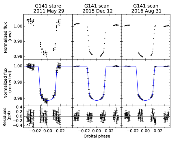
As part of the Cycle 23 HST program GO-14260 (PI: D. Deming), we obtained time-resolved spectroscopic observations during two transits of HAT-P-12b on UT 2015 December 12 and 2016 August 31 using the G141 grism (1.0–1.7 m) on WFC3. Each visit was comprised of five 96 minute HST orbits, with 45 minute gaps in data collection due to Earth occultations. The observations were carried out in spatial scan mode, with the star scanned perpendicularly to the dispersion direction across the detector at a rate of s-1. In addition, at the start of the first orbit of each visit, we obtained an undispersed direct image of the star using the F139M grism for use in wavelength calibration. Each of the 74 spectra has a total exposure time of 112 s and extends roughly 30 pixels in the spatial direction. With the SPARS25 NSAMP=7 readout mode, each image file consists of seven nondestructive reads of the entire 266266 pixel subarray. These two scan mode visits have been previously analyzed in Tsiaras et al. (2018).
We also include in our analysis an older stare mode transit observation from UT 2011 May 29 (GO-12181; PI: D. Deming) that was analyzed previously in Line et al. (2013) and Sing et al. (2016). This visit consisted of 112 12.8 s exposures over the course of four orbits. Each orbit necessitated five buffer dumps, resulting in 9 minute gaps interrupting the data collection. There are 16 nondestructive reads of the 512512 pixel subarray in each image file. When reducing the images, we treat the stare mode data in the same way as the spatial scan mode observations. The observation details for the three WFC3 visits are summarized in Table 1.
Starting with the dark- and bias-corrected *ima.fits files produced by the standard WFC3 calibration pipeline, CALWFC3, we proceed with the data reduction using the Python 2–based Exoplanet Transits, Eclipses, and Phase Curves (ExoTEP) pipeline developed by B. Benneke and I. Wong (see also Benneke et al. 2017, 2019). To achieve maximal background subtraction in the extracted spectra, we follow a standard procedure for WFC3 spatial scan image processing (e.g., Deming et al. 2013; Kreidberg et al. 2014; Evans et al. 2016): we construct subexposures by subtracting consecutive nondestructive reads and coadd all of the background-subtracted subexposures together to form the full background-corrected data frame.
The spatial extent of each subexposure is determined by calculating the median flux profile for the difference image along the scan direction, i.e., -direction, and locating the pixels where the flux falls to 20% of the maximum value. To form the subexposure, we take the data that lie between these two rows, with an extra buffer of 15 pixels on the top and bottom, while setting all other pixel values to zero. This method ensures that all of the stellar flux collected by the instrument between nondestructive reads is extracted and that the size of the extraction region for a given subexposure (e.g., difference of the third and second reads) remains largely consistent across each visit. The final results are not sensitive to the particular choice of buffer size between 10 and 20 pixels. The background level of each subexposure is set as the median of a 50 column wide region situated sufficiently far from the spectral trace and avoiding the edges of the subarray.
Due to the particular geometry of the WFC3 instrument, the first-order spectrum of the G141 grism is not perfectly parallel to the detector rows. Also, there are significant variations in the length of the spectrum in the dispersion direction across the spatial scan, which results in the wavelength associated with a particular detector column varying from the top to the bottom. Lastly, imperfections in the pointing resets between each exposure lead to small horizontal shifts in the spectra across each visit (e.g., Deming et al. 2013; Knutson et al. 2014; Kreidberg et al. 2014). Therefore, the shape of the spectrum on the detector is trapezoidal and slightly inclined relative to the subarray rows. Some previous analyses of WFC3 data have addressed this issue either by aligning the rows of the spectrum via interpolation (Kreidberg et al. 2014) or by deriving correction factors for the published wavelength calibration coefficients (Wilkins et al. 2014).
In the ExoTEP pipeline, we follow the methodology described in detail in Tsiaras et al. (2016) and compute the exact wavelength solution across the entire subarray for each exposure. In short, we first determine the position of the star along the -axis of the detector for each exposure by taking the position of the star in the direct undispersed image, adjusting for differences in reference pixel location and subarray size between the direct and spatial scan images, and calculating the horizontal offset of each spectrum relative to the first spectroscopic exposure. The offsets are calculated by computing the centroid of each exposure and measuring the horizontal shift relative to the first exposure of the visit.
Next, assuming that the spatial scan shifts the star position perfectly vertically across the detector, we determine the trace position and the wavelength solution along the trace using the calibration coefficients included in the configuration file WFC3.IR.G141.V2.5.conf (Kuntschner et al. 2009) for a range of stellar positions. After a 2D cubic spline interpolation, we can now calculate the wavelength at every location on the subarray for each exposure. We also utilize this wavelength solution to apply a wavelength-dependent flat-field correction, using the cubic flat-field coefficients listed in the calibration file WFC3.IR.G141.flat.2.fits (Kuntschner et al. 2011; Tsiaras et al. 2016).
The last step in the ExoTEP data reduction process before light-curve extraction is cosmic-ray correction. For each exposure, we calculate the normalized row-added flux template. Next, we flag outliers using moving median filters of 10 pixels in width in both the and directions. Flagged pixel values are replaced by the value in the template corresponding to its position, appropriately scaled to match the total flux in its column. The particular parameters of the median filters are manually adjusted by inspecting the final corrected images and checking that all visible outliers have been removed. Due to the narrow vertical spatial profile of the trace in the stare mode images, we only apply the bad pixel correction in the horizontal direction for that visit.
To construct the spectroscopic light curves, we define a 20 nm wavelength grid from 1.10 to 1.66 m and determine the spatial boundaries of the patch corresponding to each wavelength bin on the subarray using the previously derived wavelength solution. We calculate the flux within each patch by adding the pixel counts for all pixels that are fully within the patch and then computing the additional contribution from the partial pixels that are intersected by the patch boundaries. For each partial pixel, we integrate a local 2D cubic polynomial interpolation function over the subpixel regions that lie inside and outside of the given patch in order to compute the fraction of the total pixel count lying within the patch. This process ensures that the total flux is conserved and yields a modest reduction in the photometric scatter relative to more conventional extraction methods, which typically smooth the data in the dispersion direction prior to light-curve extraction (e.g., Deming et al. 2013; Knutson et al. 2014; Tsiaras et al. 2016).
The time stamp for each data point is set to the mid-exposure time. To produce the broadband HST WFC3 light curve (i.e., white light curve), we simply sum the flux from the full set of individual spectroscopic light curves.
| Data Set | UT Start Date | a | (s)b | Mode |
|---|---|---|---|---|
| WFC3 G141 | ||||
| Visit 1 | 2011 May 29 | 112 | 12.8 | Stare |
| Visit 2 | 2015 Dec 12 | 74 | 112 | Scan |
| Visit 3 | 2016 Aug 31 | 74 | 112 | Scan |
| STIS G430L | ||||
| Visit 1 | 2012 Apr 11 | 34 | 280 | |
| Visit 2 | 2012 Apr 30 | 34 | 280 | |
| STIS G750L | ||||
| Visit 1 | 2013 Feb 4 | 34 | 280 |
-
•
Notes.
-
•
aTotal number of exposures
-
•
bTotal integration time per exposure
| Dataset | UT Start Date | a | (s)b | (minutes)c | c | c | c | Binningd |
|---|---|---|---|---|---|---|---|---|
| 3.6 m | ||||||||
| Transit | 2013 Mar 8 | 8064 | 1.92 | 0 | 2.5 | 1.5 | 64 | |
| Eclipse 1 | 2010 Mar 16 | 2097 | 10.4 | 60 | 3.0 | 2.0 | 16 | |
| Eclipse 2 | 2014 Apr 15 | 9024 | 1.92 | 30 | 4.0 | 1.0 | 16 | |
| 4.5 m | ||||||||
| Transit | 2013 Mar 11 | 8064 | 1.92 | 0 | 3.0 | 1.6 | 128 | |
| Eclipse 1 | 2010 Mar 26 | 2097 | 10.4 | 45 | 3.5 | 2.5 | 32 | |
| Eclipse 2 | 2014 May 8 | 9024 | 1.92 | 60 | 2.5 | 2.4 | 128 |
-
•
Notes.
-
•
aTotal number of images.
-
•
bTotal integration time per image.
-
•
cHere is the amount of time trimmed from the start of each time series prior to fitting, is the radius of the aperture used to determine the star centroid position, and is the radius of the aperture used to compute the noise pixel parameter . The column denotes how the photometric extraction aperture is defined. All radii are given in units of pixels. When using a fixed aperture, the noise pixel parameter is not needed, so is undefined. See text for more details.
-
•
dNumber of data points placed in each bin when binning the photometric series prior to fitting.
2.2. HST STIS
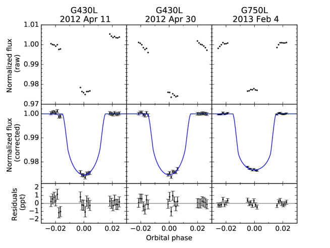
We observed three transits of HAT-P-12b with the HST STIS instrument as part of the program GO-12473 (PI: D. Sing). Observations of two transits were carried out using the G430L grating (290–570 nm) on UT 2012 April 11 and 30; the third transit was observed using the G750L grating (550–1020 nm) on UT 2013 February 4. The two gratings used have resolutions of (5.5 and 9.8 Å per 2 pixel resolution element for the G430L and G750L gratings, respectively). Each visit contains a total of 34 science exposures across four HST orbits, with the third orbit occurring during mid-transit. To reduce overhead, data were read out from a 1024128 subarray with a per-exposure integration time of 280 s. The observational details for the three STIS visits are listed in Table 1. This set of observations has been analyzed in two previous independent studies: Sing et al. (2016) and Alexoudi et al. (2018).
The raw images are flat-fielded using the latest version of CALSTIS. The subsequent data reduction is completed using the ExoTEP pipeline. We remove outlier pixel values in the time series by first computing the median image across each visit and then replacing all pixel values in the individual exposure frames varying by more than with the corresponding value in the median image. We apply the wavelength solution provided in the *sx1.fits calibrated files and extract the column-added 1D spectra, choosing the aperture width and whether to subtract the background so as to minimize the scatter in the residuals from the transit light-curve fit (e.g., Deming et al. 2013). In our analysis of the two G430L observations, we utilize 9 and 7 pixel wide apertures, respectively, removing the background for the first visit only; in the case of the G750L transit, we find that extracting spectra from a 7 pixel wide aperture after background subtraction results in the minimum scatter.
Data collected using the G750L grism suffer from a fringing effect, which manifests itself as an interference pattern superposed on the 1D spectrum and is especially apparent at wavelengths longer than 700 nm. Following the methods outlined in previously published analyses of data from this program (e.g., Nikolov et al. 2014, 2015; Sing et al. 2016), we defringe our data using a fringe flat frame obtained at the end of the G750L science observations.
Lastly, we correct for subpixel wavelength shifts in the dispersion direction across each visit by fitting for the horizontal offsets and amplitude scaling factors that align all extracted spectra with the first one. The normalized broadband light curve is simply the time series of the optimized amplitude scaling factors. To generate the spectroscopic light curves, we collect the flux within 200 and 100 pixel bins for the G430L and G750L observations, respectively. The wavelength bounds corresponding to the 200 pixel bins for the two G430L transit observations differ by less than the characteristic wavelength resolution element (0.55 nm). For the G750L dataset, we also include two narrow wavelength bins centered around the sodium and potassium absorption lines (588.7–591.2 and 770.3–772.3 nm respectively).
2.3. Spitzer IRAC
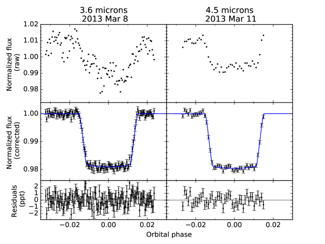
Two transits of HAT-P-12b were observed in the 3.6 and 4.5 m broadband channels of the Infrared Array Camera (IRAC) on the Spitzer Space Telescope (Program ID 90092; PI: J.-M. Désert). The observations took place on UT 2013 March 8 and 11 and were carried out in subarray mode, which produces 3232 pixel () images centered on the stellar target. Each transit observation is comprised of 8064 images with a per-exposure effective integration time of 1.92 s.
A set of two secondary eclipse observations, one in each of the two postcryogenic IRAC channels, was obtained on UT 2010 March 16 and 26 (Program ID 60021; PI: H. Knutson). These data consist of 2097 images per passband obtained in full array mode at a resolution of 256256 pixels () with an effective exposure time of 10.4 s per image. Peak-up pointing was utilized, which entails an initial 30 minute observation prior to the start of the science observation to allow for the stabilization of the telescope pointing. These eclipses were previously analyzed in Todorov et al. (2013). A second set of hitherto unpublished secondary eclipse observations, including one in each channel, was obtained on UT 2014 April 15 and May 8 (Program ID 10054; PI: H. Knutson). These observations were taken in subarray mode with peak-up pointing and contain 9024 images with effective exposure times of 1.92 s.
We extract photometry following the techniques described in detail in previous analyses of postcryogenic Spitzer data (e.g., Knutson et al. 2012; Lewis et al. 2013; Todorov et al. 2013; Wong et al. 2015, 2016). Starting with the dark-subtracted, flat-fielded, linearized, and flux-calibrated images produced by the standard IRAC pipeline, we calculate the sky background via a Gaussian fit to the distribution of pixel values, excluding pixels near the star and its diffraction spikes, as well as the problematic top (32nd) row, which has flux values that are systematically lower than the other rows. We also iteratively trim outlier pixel values on a pixel-by-pixel basis using a moving median filter across the adjacent 64 images in the time series.
The position of the star on the detector is determined using the flux-weighted centroiding method (e.g., Knutson et al. 2012). The width of the star’s point response function (PRF; i.e., the convolution of the star’s point-spread function and the detector response function) is estimated by computing the noise pixel parameter (see Lewis et al. 2013 for a full discussion). The stellar position and PRF width are calculated using circular apertures of radius and , respectively, which we vary in 0.5 pixel steps to produce different versions of the extracted photometry. The photometric series can be extracted using both fixed and time-varying circular apertures, where in the case of time-varying apertures, the radii are related to the square root of the noise pixel parameter by either a constant scaling factor or a constant shift (e.g., Wong et al. 2015, 2016).
Prior to fitting (see Section 3), we can bin the photometric series into various intervals equal to powers of two (i.e., 1, 2, 4, 8, etc. points). To aid in the removal of instrumental systematics, we also experiment with trimming the first 15, 30, 45, or 60 minutes of data from the time series. Before fitting each photometric series with our transit/eclipse light-curve model, we apply an iterative moving median filter of 64 data points in width to remove points with measured fluxes, or star centroid positions, or values that vary by more than 3 from the corresponding median values. For all Spitzer datasets, the number of removed points is less than 5% of the total number of data points, and slightly altering the width of the median filter does not significantly affect the number of removed points.
For each transit or secondary eclipse observation, we determine the optimal aperture and photometric parameters by fitting the various photometric series with the model light curve and selecting the version that minimizes the scatter in the resultant residuals, binned in 5 minute intervals (Wong et al. 2015, 2016). The optimal values are listed in Table 2.
2.4. Photometric monitoring for stellar activity
High levels of chromospheric activity, which can lead to significant photometric variability and incur wavelength-dependent biases in the measured transmission spectrum (e.g., Rackham et al. 2018), can be displayed by K dwarfs such as HAT-P-12. In particular, the presence of unocculted starspots can impart slope changes to the shape of the transmission spectrum in the optical, affecting the interpretation of the planet’s atmospheric properties.
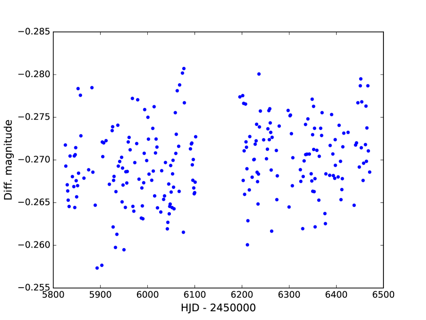
To characterize the level of stellar activity on HAT-P-12, we obtained Cousins -band photometry of the star using the the Tennessee State University Celestron 14 inch (C14) Automated Imaging Telescope (AIT) located at Fairborn Observatory, Arizona. Differential magnitudes of HAT-P-12 were calculated relative to the mean brightnesses of five constant comparison stars from five to ten co-added consecutive exposures. Details of our observing, data reduction, and analysis procedures with the AIT are described in Sing et al. (2015).
A total of 237 successful nightly observations were collected across two observing seasons (season 1: 2011 September 20–2012 June 22; season 2: 2012 September 24–2013 June 26). The individual observations are plotted in Figure 1. The seasonal means in differential magnitude are and , with corresponding single observation standard deviations of 0.0046 and 0.0042, respectively. These scatter values are comparable to the approximate limit of the measurement precision. This indicates that HAT-P-12 does not show any significant variability.
When performing a periodogram analysis of individual seasonal datasets, we do not retrieve any frequencies that produce amplitudes larger than the seasonal standard deviations. In particular, we do not detect a variability signal with a period near the estimated rotational period of the star ( days; Mancini et al. 2018). Such a periodicity in the photometry would be indicative of rotational modulation of weak features on the stellar surface. We therefore conclude that HAT-P-12 is a very quiescent host star.
This conclusion is consistent with the findings from high-resolution spectroscopy of the host star during the initial discovery and characterization of the system (Hartman et al. 2009), which did not detect significant levels of variability suggestive of large starspots across the stellar surface. Analyses of stellar spectra from the Keck High Resolution Echelle Spectrometer (HIRES) and more recently from the High Accuracy Radial Velocity Planet Searcher (HARPS) instrument also indicate low stellar activity as determined by the Ca II H and K lines: (Knutson et al. 2010) and (Mancini et al. 2018). In addition, none of the transit light curves analyzed in this work show evidence for occulted spots.
It is notable that HAT-P-12b has an optical transmission spectrum that shows a slope indicative of Rayleigh scattering (Sing et al. 2016; Alexoudi et al. 2018 and this work), while the host star has low stellar activity. This is in contrast to the paradigmatic case of HD 189733b, which has a clear optical scattering slope and an active host star. Thus, HAT-P-12b serves as an important test of whether the transmission slope is related to stellar activity, which could happen in the case of unocculted stellar spots or with enhanced photochemistry as a product of higher stellar far- and near-UV levels.
3. Analysis
We carry out a global analysis of all eight transit light curves (three HST WFC3 G141 visits, two HST STIS G430L visits, one HST STIS G750L visit, and two Spitzer IRAC visits at 3.6 and 4.5 m) by simultaneously fitting our transit light-curve model, instrumental systematics models, and photometric noise parameters using the ExoTEP pipeline (Benneke et al. 2017, 2019). We also perform an independent combined fit of the four Spitzer secondary eclipse light curves.
3.1. Broadband Light-Curve Fits
3.1.1 Instrumental Systematics
Prior to fitting the HST WFC3 light curves, we discard the first orbit, as well as the first two exposures of each orbit, which notably improves the resultant fits. We also remove the 31st and 68th exposures, which were affected by cosmic ray hits, from the second spatial scan mode transit light curve.
Raw uncorrected light curves obtained using the HST WFC3 instrument exhibit well-documented systematic flux variations across the visit, as well as within each individual spacecraft orbit (e.g., Deming et al. 2013; Kreidberg et al. 2014). We model the HST WFC3 instrumental systematics with the following analytical function (e.g., Berta et al. 2012; Kreidberg et al. 2015):
| (1) |
Here is a normalization constant, is the visit-long slope, and are the rate constant and amplitude of the orbit-long exponential ramps, and and are the time elapsed since the beginning of the visit and since the beginning of the orbit, respectively. Here is set to a constant for points in the first fitted orbit and zero everywhere else, reflecting the observed difference in the ramp amplitude between the first fitted orbit and the subsequent orbits.
We find that stare mode observations exhibit an additional quasi-linear systematic trend across exposures taken between each buffer dump (five per orbit for our visit). We can correct for this trend by appending an extra factor of to Eq. (1), where is the linear slope, and is the time elapsed since the end of the last buffer dump.
Similar ramp-like instrumental systematics are also apparent in HST STIS raw light curves, albeit with a somewhat different shape. We correct these systematics using a standard analytical model (Sing et al. 2008),
| (2) |
where , , , and are defined in the same way as in Eq. (1), and the coefficients describe the fourth-order polynomial shape of the orbit-long trend. As with the HST WFC3 light curves, we remove the first orbit, as well as the first two exposures of each orbit prior to fitting.
Raw photometry obtained using the Spitzer IRAC instrument is characterized by short-timescale variations in the measured flux due to small oscillations of the telescope pointing and nonuniform sensitivity of the detector at the subpixel scale. We correct for these intrapixel sensitivity variations by using the modified version of the Pixel Level Decorrelation method (PLD; Deming et al. 2015) described in Benneke et al. (2017):
| (3) |
The arrays represent the pixel counts for the nine pixels located in a box centered on the star’s centroid position normalized to sum to unity at each point in the time series. These normalized pixel count arrays are placed into a linear combination with weights . The last term models a visit-long linear trend, where is the slope parameter and denotes the time elapsed since the beginning of the time series. As with the photometric series, the pixel count arrays can be binned prior to fitting. We optimize for the binning interval and the number of points trimmed from the start of the observation by carrying out individual fits of each IRAC transit light curve (see Section 2.3). In the global transit light-curve fit, no additional alterations of the IRAC light curves are needed.
| Parameter | Instrument | Wavelength (nm) | Value |
|---|---|---|---|
| Planet radius, | STIS G430L | 289–570 | |
| Planet radius, | STIS G750L | 526–1025 | |
| Planet radius, | WFC3 G141 | 920–1800 | |
| Planet radius, | IRAC 3.6 m | 3161–3928 | |
| Planet radius, | IRAC 4.5 m | 3974–5020 | |
| Transit center time, (BJDTDB) | |||
| Period, (days) | |||
| Impact parameter, | |||
| Inclination,a (deg) | |||
| Relative semimajor axis, |
-
•
Note. aInclination derived from impact parameter via .
3.1.2 Limb Darkening
The ExoTEP pipeline incorporates the Python-based package LDTK (Parviainen & Aigrain 2015) to automatically calculate limb-darkening coefficients. Given the literature values and uncertainties for the stellar parameters ( K, , ; Hartman et al. 2009), this program generates a mean limb-darkening profile and profile uncertainties for each specified bandpass (broadband or spectroscopic) via Monte Carlo sampling of interpolated nm PHOENIX stellar intensity spectra (Husser et al. 2013) within a range in the space of the three stellar parameters.
Subsequent maximum-likelihood optimization returns the best-fit linear, quadratic, or nonlinear limb-darkening coefficients to be used in calculating the transit shape in each bandpass. In our global fit, we find that using the four-parameter nonlinear limb-darkening model yields the lowest residual scatter during ingress and egress, particularly for the high signal-to-noise HST WFC3 spatial scan mode visits.
Because the custom stellar spectra accessed by the LDTK package do not cover wavelengths longer than 2.6 m, we set the limb-darkening coefficients for the Spitzer IRAC 3.6 and 4.5 m transit light curves to the values computed following the methods described in Sing (2010). These coefficients are tabulated online111pages.jh.edu/dsing3/David_Sing/Limb_Darkening.html for a wide range of (, , ) values, and we choose the values listed for the set of stellar parameters closest to the literature values for HAT-P-12.
To empirically verify that our choice of fixing limb-darkening coefficients to modeled or tabulated values does not have a significant effect on the measured transmission spectrum, we have experimented with fitting for quadratic limb-darkening coefficients in individual fits of the WFC3 scan mode visits and the broadband Spitzer transit light curves; these visits have either complete transit coverage or the highest per-point precision. We find that the fitted coefficients have large relative uncertainties (20%–70%), i.e., are not well constrained by the data, while being statistically consistent with the corresponding values produced by LDTK or listed in the Sing (2010) tables. Crucially, no significant shifts in transit depth occur when switching from fixed limb-darkening coefficients to fitted values.
3.1.3 Global Fit Results
| Wavelength (nm) | |
|---|---|
| STIS G430L | |
| 346–401 | |
| 401–456 | |
| 456–511 | |
| 511–565 | |
| STIS G750L | |
| 528–577 | |
| 577–626 | |
| 626–675 | |
| 675–723 | |
| 723–772 | |
| 772–821 | |
| 821–870 | |
| 870–919 | |
| 919–968 | |
| 968–1016 | |
| 588.7–591.2 (Na)a | |
| 770.3–772.3(K)a | |
| WFC3 G141 | |
| 1100–1120 | |
| 1120–1140 | |
| 1140–1160 | |
| 1160–1180 | |
| 1180–1200 | |
| 1200–1220 | |
| 1220–1240 | |
| 1240–1260 | |
| 1260–1280 | |
| 1280–1300 | |
| 1300–1320 | |
| 1320–1340 | |
| 1340–1360 | |
| 1360–1380 | |
| 1380–1400 | |
| 1400–1420 | |
| 1420–1440 | |
| 1440–1460 | |
| 1460–1480 | |
| 1480–1500 | |
| 1500–1520 | |
| 1520–1540 | |
| 1540–1560 | |
| 1560–1580 | |
| 1580–1600 | |
| 1600–1620 | |
| 1620–1640 | |
| 1640–1660 |
-
•
Note.
-
•
aNarrow wavelength bins centered on the alkali (Na and K) absorption lines.
In our pipeline, the transit shape is calculated using the BATMAN package (Kreidberg 2015). For the global broadband light-curve analysis, we fit for a separate transit depth () in each of the five bandpasses (STIS G430L, STIS G750L, WFC3 G141, IRAC 3.6 m, and IRAC 4.5 m), along with a single set of transit geometry parameters (, ) and transit ephemerides (, ) for all light curves.
The log-likelihood function for our joint light-curve fits is
| (4) |
where the outer summation goes over all visits. For each visit , is the number of data points , is the appropriate instrumental systematics model (Section 3.1.1), is the transit light-curve model, and is a free photometric noise parameter. We have introduced an independent noise parameter for each visit to account for differences in the level of scatter across the various transit light curves. The best-fit values of the noise parameters establish conservative estimates of the photometric uncertainty on each data point.
The ExoTEP pipeline simultaneously computes the best-fit values and uncertainties for all astrophysical and systematics model parameters using the affine-invariant Markov Chain Monte Carlo (MCMC) ensemble sampler emcee (Foreman-Mackey et al. 2013). To facilitate convergence of the chains, we initialize the global fit with the best-fit values calculated by fitting each transit individually. The global transit fit contains a total of 53 free astrophysical, systematics, and noise parameters. We use walkers and chain lengths of 20,000 steps, discarding the first 60% of each chain when computing the posterior distributions of the fit parameters. To check for convergence, we run the fit five times and ensure that the parameter estimates are consistent across the five runs at better than the level. The results of our global transit light-curve analysis are listed in Table 3. Plots of the best-fit transit light curves and their corresponding residuals are shown in Figures 2–4.
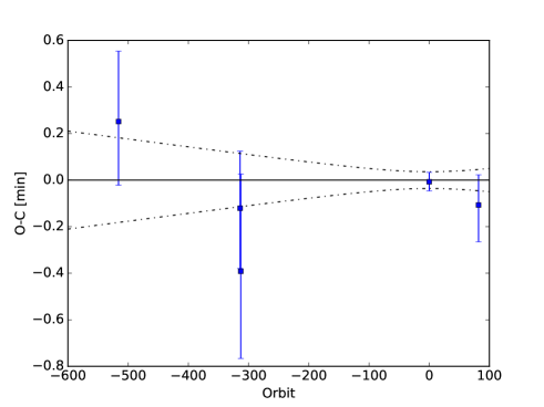
Our global fits assume a single transit ephemeris across all visits, as well as a common transit depth for visits observed in the same bandpass. To validate this treatment, we also analyze each visit individually in order to compare the best-fit transit timings with the global best-fit transit ephemeris and ensure consistent transmission spectrum shapes among the visits. Figure 5 shows the calculated transit times for individual visits relative to the best-fit global transit ephemeris; only visits with full transit coverage or partial coverage including ingress and egress are included. All of the individual transit times agree with the global ephemeris at better than the level, ruling out any statistically significant transit timing variation.
3.2. Spectroscopic Light-curve Fits
When fitting the individual spectroscopic light curves in the STIS G430L, STIS G750L, and WFC3 G141 bandpasses, we fix the transit geometry parameters and transit ephemeris to the best-fit values from the global broadband transit analysis (Table 3), with the transit depth being the only free astrophysical parameter.
The ExoTEP pipeline offers a choice of three methods for defining the instrumental systematics model for the constituent spectroscopic light curves. The first method utilizes the full systematics model for the corresponding instrument, computing the best-fit instrumental systematics parameters for each spectroscopic light curve independently from the broadband light curve. The other methods apply a common-mode correction to the spectrophotometric series prior to fitting, dividing each series by either (1) the best-fit broadband systematics model (e.g., Kreidberg et al. 2014), or (2) the ratio of the uncorrected broadband photometric series and the best-fit broadband transit model (e.g., Deming et al. 2013).
Performing a precorrection on the spectroscopic light curves takes advantage of the more well-defined systematics model derived using the high signal-to-noise broadband light curves. This technique also enables us to use fewer systematics parameters in the individual spectroscopic light-curve fits, which typically results in tighter constraints on the best-fit transit depths. We account for residual systematic flux variations in the spectroscopic light curves using a simplified model,
| (5) |
which describes a linear function with respect to the measured subpixel shifts in the dispersion direction relative to the first exposure in the time series, with and being the offset and slope parameters, respectively.
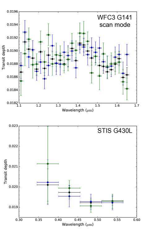
To demonstrate consistency in the transmission spectrum shape between separate observations in the same bandpass, we first analyze the spectroscopic light curves of individual visits. Figure 6 shows the transmission spectra of the individual WFC3 G141 scan mode and STIS G430L visits plotted with the corresponding spectra derived from the joint analysis. In both cases, there is good agreement between the individual transit depths in each wavelength bin, and the spectrum shapes are consistent across the visits. In particular, each WFC3 G141 scan mode visit spectrum shows a discernible absorption feature at 1.4 m. It is also important to note that this feature was not detected in the older stare mode data analyzed in Line et al. (2013), which underscores the significant improvement in sensitivity provided by the scan mode observations.
Using the same log-likelihood expression as in our global broadband transit light-curve fit (Eq. (3.1.3)), we then fit all visits in a given bandpass jointly, letting the systematics model and photometric noise parameters vary independently for each light curve. For the STIS G430L and G750L spectroscopic light curves, in line with similar previous studies (e.g., Sing et al. 2016), we find that the shapes of the systematic trends vary significantly across the various wavelength bins, necessitating the use of the full systematics model. Meanwhile, the HST WFC3 systematics are largely independent of wavelength and detector position, and we find that the two precorrection strategies described above result in fits of comparable quality. In this paper, we report the best-fit depths derived from using the latter of the two precorrection methods (i.e., dividing the ratio of the uncorrected flux and the best-fit transit model from the broadband light curve).
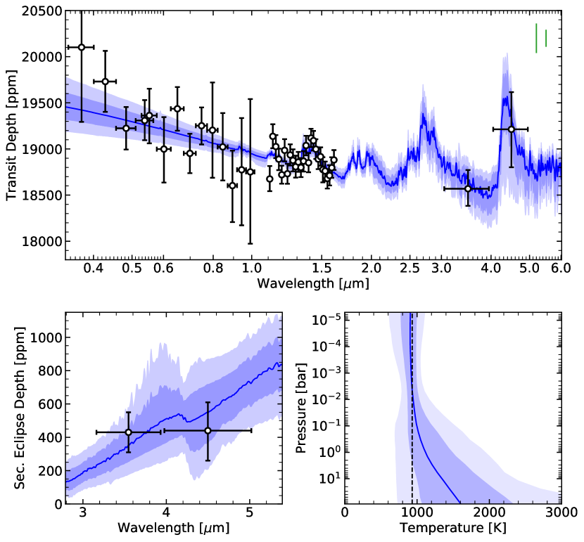
The results of our spectroscopic light-curve fits are listed in Table 4. The best-fit transit light curves and associated residuals are plotted in the Appendix for each of the HST STIS and WFC3 visits. When experimenting with different wavelength bin widths (10–40 nm), we get consistent transmission spectrum shapes. Visual inspection of the systematics-corrected light curves does not reveal any salient outliers or residual uncorrected systematics trends. We combine the transit depths from the spectroscopic light-curve fits with the broadband Spitzer IRAC transit depths to construct the full transmission spectrum of HAT-P-12b, which is plotted in Figure 7. The transit depths for the narrow wavelength bins in the main alkali absorption regions are consistent with the depths measured in the wider bins spanning those regions, indicating a nondetection of the alkali absorption; these data points are not shown in the transmission spectrum plot. The primary features of the transmission spectrum are the Rayleigh slope extending through the optical bandpasses and a small absorption feature around 1.4 m indicative of water vapor. These observations together suggest the presence of both uniform clouds and fine-particle scattering in the atmosphere of HAT-P-12b.
The shape of the transmission spectrum at visible wavelengths matches the results of previous analyses of the HST STIS data by Sing et al. (2016) and Alexoudi et al. (2018). It is worth mentioning that an earlier study of HAT-P-12b’s atmosphere using ground-based broadband photometry produced a flat transmission spectrum throughout the visible wavelength range (Mallonn et al. 2015), consistent with an opaque layer of clouds as opposed to Rayleigh scattering. This discrepancy was discussed in Alexoudi et al. (2018) and attributed to uncertainties in the inclination and semi-major axis of HAT-P-12b’s orbit, which are correlated with transit depths and can yield wavelength-dependent shifts that alter the apparent transmission spectrum slope in the optical.
When assuming different values of and in reanalyzing the Mallonn et al. (2015) light curves, Alexoudi et al. (2018) were able to recover a discernible Rayleigh scattering slope in the visible transmission spectrum. In our global fit, we take advantage of the well-sampled ingress and egress from the scan mode HST WFC3 and Spitzer light curves to place much narrower constraints on and than these earlier studies. Therefore, our results are a robust validation of the previously published reports of a negative slope in the visible transmission spectrum of HAT-P-12b.
3.3. Secondary Eclipses
The eclipse light curve is defined in the same way as a transit light curve but without the limb-darkening effect. We utilize the same modified PLD instrumental systematics model to account for the Spitzer IRAC intrapixel sensitivity variations (Eq. (3)). For each eclipse observation, we select the optimal aperture, photometric parameters, binning, and trimming by fitting the eclipse light curve individually, fixing the transit geometry parameters (, ) and transit ephemerides (, ) to the best-fit values from the global broadband transit light-curve analysis (Table 3).
When performing individual eclipse fits on the relatively low signal-to-noise data, we facilitate comparison between different versions of the photometry/binning/trimming by fixing the time of eclipse to an orbital phase of 0.5. The orbital phase here is defined relative to the best-fit ephemeris from the global transit fit. To correct for any residual flux ramps at the start of the data, we also experiment with including an exponential factor in the systematics model, where and are the amplitude and time constant, respectively, and is the time elapsed since the beginning of the time series. Following Wong et al. (2015, 2016), we choose the photometric series that produce the lowest residual scatter. Only for the first 3.6 m eclipse dataset does the inclusion of a ramp appreciably improve the fit (i.e., minimizes the value of the Bayesian Information Criterion).
We also carry out a global analysis of all four secondary eclipse observations. In this fit, we allow the instrumental systematics parameters for each dataset to vary independently while assuming common 3.6 and 4.5 m eclipse depths and center of eclipse phase as free parameters. The results of our individual and global eclipse fits are listed in Table 5. The raw and systematics-corrected eclipse light curves are shown in Figure 8. From the individual fits, we only find marginal eclipse detections for the full array 3.6 and 4.5 m visits (), while the more recent subarray observations yield more robust detections (). The best-fit eclipse phase from the combined analysis is consistent with a circular orbit, and the global 3.6 and 4.5 m depths are statistically consistent with each of the individual best-fit eclipse depths at better than the level.

| Eclipse | Depth (%) | Phase |
|---|---|---|
| 3.6 m | ||
| Eclipse 1 | a | |
| Eclipse 2 | ||
| Globalb | ||
| 4.5 m | ||
| Eclipse 1 | ||
| Eclipse 2 | ||
| Globalb |
-
•
Notes.
-
•
aThe eclipse phase was fixed at 0.5 for all individual eclipse fits, assuming the best-fit orbital ephemeris from the global transit fit (Table 3).
-
•
bComputed from a simultaneous fit of all four eclipses.
4. Atmospheric Retrieval
We simultaneously interpret the full transmission and emission spectra presented in this work to deliver quantitative constraints on the atmosphere of HAT-P-12b using the SCARLET atmospheric retrieval framework (Benneke & Seager 2012, 2013; Kreidberg et al. 2014; Knutson et al. 2014; Benneke 2015; Benneke et al. 2019). Employing SCARLET’s chemically consistent mode, we define the atmospheric metallicity, the C/O ratio, the cloud properties, and the vertical temperature structure as free parameters. SCARLET then determines their posterior constraints by combining a chemically-consistent atmospheric forward model with a Bayesian MCMC analysis. We perform the retrieval analysis with 100 walkers using uniform priors on all the parameters and run the chains well beyond formal convergence to obtain smooth posterior distribution even near the contours.
To evaluate the likelihood for a particular set of atmospheric parameters, the SCARLET forward model in chemically consistent mode first computes the molecular abundances in chemical and hydrostatic equilibrium and the opacities of molecules and Mie-scattering clouds (Benneke & Seager 2013). The elemental composition in the atmosphere is parameterized using the atmospheric metallicity, [M/H], and the atmospheric C/O ratio. We employ log-uniform priors, and we consider the line opacities of H2O, CO, and CO2 from HiTemp (Rothman et al. 2010) and CH4, NH3, HCN, H2S, C2H2, O2, OH, PH3, Na, K, TiO, SiO, VO, and FeH from ExoMol (Tennyson et al. 2012), as well as the collision-induced absorption of H2 and He.
Following Benneke et al. (2019), we use a three-parameter Mie-scattering cloud description for the retrieval analysis defining the mean particle size , the pressure level at which the clouds become optically opaque to grazing starlight at 1.5 m, and the scale height of the cloud profile relative to the gas pressure scale height as free parameters. All free parameters are allowed to vary independently in the retrieval. When calculating the cloud opacity, the retrieval is agnostic to the particular composition of the spherical cloud particles, considering only their size and vertical distribution; the former is assumed to be a logarithmic Gaussian distribution with a fixed width of . This three-parameter cloud description is motivated by the information content of transmission spectra and captures the wavelength-dependent opacities of a wide range of finite-sized cloud particles near the cloud deck in a highly orthogonal way, ideal for retrieval (Benneke et al. 2019). It reduces to Rayleigh hazes in the limit of small particles and a gray cloud deck for large particles while simultaneously allowing for any finite-sized Mie-scattering particles in between. We employ log-uniform priors on the three cloud parameters.
Our temperature structure is parameterized using the five-parameter analytic model from Parmentier & Guillot (2014) augmented with a constraint on the plausibility of the total outgoing flux. Given the relatively weak constraints on the atmospheric composition, we conservatively ensure the plausibility of the temperature structure by enforcing that the wavelength-integrated outgoing thermal flux is consistent with the stellar irradiation, a Bond albedo between 0 and 0.7, and heat redistribution values between full heat redistribution across the planet and no heat redistribution. In the retrieval, we parameterize only one temperature structure for both the dayside and the terminator because the retrieved temperature uncertainties are hundreds of K and the precision of the transmission spectrum does not justify additional parameters describing the terminator temperature structure separately.
Finally, high-resolution synthetic transmission and emission spectra are computed using line-by-line radiative transfer and integrated over the appropriate instrument response functions before being compared to the observations. Sufficient wavelength resolution in the synthetic spectra is ensured by repeatedly verifying that the likelihood for a given model is not significantly affected by the finite wavelength resolution (). Reference models are computed at .
| Parameter | Value | Unit |
|---|---|---|
| Atmospheric metallicity, | x solar | |
| Atmospheric C/O ratio | ||
| Mean particle size,a | m | |
| Opacity pressure level,b | mbar | |
| Relative cloud scale height,c | ||
-
•
Notes.
-
•
aMean particle size, assuming a logarithmic Gaussian distribution with fixed width of
-
•
bPressure at transmission optical depth of unity at 1.5 m
-
•
cScale height of cloud profile relative to gas pressure scale height
4.1. Retrieval results
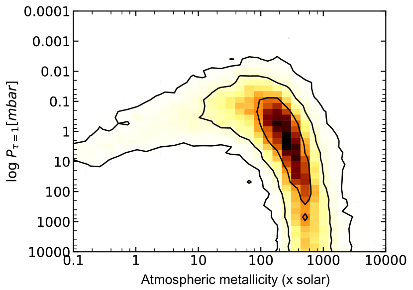
We run a set of retrievals that assume chemical and thermal equilibrium, setting the atmospheric metallicity , atmospheric C/O ratio, and cloud properties (, , and ) as free parameters. The range of representative atmospheric models derived from the retrievals is illustrated in Figure 7. The median atmospheric model is shown by the blue curve, and the and credible intervals are indicated by the shaded regions. In short, both the observed transmission and emission spectra are well fit across all wavelengths by cloudy atmospheres with cloud-top pressures between 0.2 mbar and 0.4 bar ( bounds) and supersolar metallicities. The data favor submicron cloud particle sizes, and the posterior spans most of the assumed prior range below 200 nm. Crucially, the retrieved particle sizes cover the range necessary to produce the Rayleigh scattering in the optical evident in the transmission spectrum, consistent with a previous retrieval of the HAT-P-12b atmosphere (Barstow et al. 2017). The list of parameter estimates is given in Table 6.
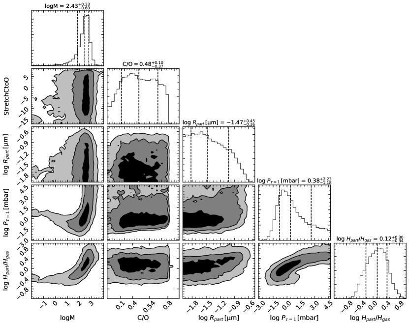
The full triangle plot displaying all one- and two-parameter marginalized posteriors is shown in Figure 9. Of particular interest is the degeneracy between cloud-top pressure and atmospheric metallicity, which is shown separately in Figure 10. Overall, the atmospheric metallicity is not well constrained: the L-shaped posterior indicates that while the data are largely consistent with cloudy atmospheres spanning a wide range of supersolar metallicities, clear atmospheres with strongly enhanced metallicities above 100 times solar cannot be ruled out at the level. This degeneracy is a common feature in atmospheric retrievals of exoplanet transmission spectra with weak or undetected 1.4 m water features (e.g., HAT-P-11b; Fraine et al. 2014), where the small magnitude of the water absorption can be caused either by attenuation due to the presence of clouds or by an intrinsically weak absorption from a hydrogen-depleted atmosphere with high mean molecular weight.
Core accretion models predict a trend of increasing bulk metallicity with decreasing planet mass (e.g., Mordasini et al. 2012; Fortney et al. 2013), and most known gas giant exoplanets have supersolar bulk metallicities (e.g., Thorngren et al. 2016). Meanwhile, the relationship between bulk and atmospheric metallicity is more complex. From planet evolution and interior structure modeling, Thorngren & Fortney (2019) predicted a 95% atmospheric metallicity upper limit of 82.3 for HAT-P-12b, broadly consistent with the results of our atmospheric retrievals and the corresponding bulk metallicity of the planet. Further enrichment of the atmospheric metallicity can result from secondary processes such as core erosion (e.g., Wilson & Militzer 2012; Madhusudhan et al. 2016) and accretion of solid material during the late stages of planet formation (e.g., Pollack et al. 1996). The atmospheric metallicity of HAT-P-12b is also comparable to similarly sized sub-Saturn planets, such as WASP-39b (100–200 solar; Wakeford et al. 2017) and WASP-127b (10–40 solar; Spake et al. 2019). Given this context, the elevated metallicity of HAT-P-12b is not entirely unexpected.
Another notable result from the retrievals is the near-solar atmospheric C/O ratio of , with a upper limit at roughly 0.83. The presence of a water vapor absorption feature at 1.4 m rules out carbon-dominated atmospheres, because the formation of H2O becomes disfavored as C/O approaches unity. The absence of a 1.15 m absorption in the WFC3 bandpass comparable in magnitude to the observed 1.4 m feature also supports the conclusion of an oxygen-dominated chemistry by eliminating CH4 as the molecular species responsible for the near-infrared absorption features (e.g., Benneke 2015). Methane has a strong absorption feature at around 3.3 m, so it follows that the relatively low transit depth measured in the Spitzer 3.6 m bandpass in comparison with the 4.5 m depth likewise points toward a near-solar C/O ratio.
In addition to the chemical and thermal equilibrium retrievals, we run a set of “free” atmospheric retrievals that do not assume chemical or thermal equilibrium; instead, the abundance of each molecular gas species is independently varied, in addition to the previously defined parameters describing the clouds. In these runs, we focus on H2O, CH4, CO, and CO2 as the primary atmospheric components to be constrained. We do not find any notable constraints on the abundances of the carbon-bearing species relative to H2O.
5. Comparison to Microphysical Cloud Models
In addition to the atmospheric retrievals presented in the previous section, we use the Community Aerosol and Radiation Model for Atmospheres (CARMA) to simulate condensation clouds and photochemical hazes in the atmosphere of HAT-P-12b. CARMA is a time-stepping cloud microphysics model that computes the bin-resolved particle size distributions of aerosols as a function of altitude in planetary atmospheres. CARMA treats aerosol formation and evolution as a kinetic processes, with convergence dictated by balancing the rates of particle nucleation, condensational growth and evaporation, coagulation, and transport via sedimentation, advection, and diffusion calculated from classical theories of cloud physics (Pruppacher & Klett 1978). It is thus significantly different from phase equilibrium models, such as Ackerman & Marley (2001), which do not consider the time evolution of the rates of microphysical processes. The specific physical formalism used in the model is described in full in the Appendix of Gao et al. (2018).
By comparing the CARMA simulation results to the observations, we hope to gain a more physical understanding of the processes controlling aerosol distributions. In our modeling of the HAT-P-12b atmosphere, we consider both condensate clouds and photochemical hazes separately. We refer the reader to the Appendix for a detailed description of the condensate and aerosol modeling setup in CARMA. For each model run, the temperature–pressure profile of the background atmosphere is set to the best-fit profile from the atmospheric retrieval (Section 4 and Figure 7). Vertical mixing of condensate or haze particles is driven by eddy diffusion, and we consider eddy diffusion coefficient values of , , , and cm2 s-1. The atmospheric metallicity is set to 10, 100, or 1000 solar; adjusting the metallicity affects the initial abundance of condensate species in the model, as well as the atmospheric scale height.
Given the uncertainties in the specific chemical pathways and efficiencies of haze production, CARMA does not carry out an ab initio haze formation calculation but instead sets the haze production rate as a free parameter. We consider haze production rates of , , and g cm-2 s-1 at a pressure of 1 bar, consistent with the values computed in exoplanet photochemical studies (e.g., Venot et al. 2015; Lavvas & Koskinen 2017; Kawashima & Ikoma 2018; Lines et al. 2018a; Adams et al. 2019). We investigate the impact of different haze compositions on the atmospheric opacity by considering different refractive indices. In particular, we consider both soots, which are expected to survive at the high temperatures of exoplanet atmospheres due to their relatively low volatility, and tholins, which we use as a proxy for lower-temperature organic hazes (Morley et al. 2015).
We find that haze models match the observed transmission spectrum much better than condensate cloud models. While many of the condensate cloud models are able to reproduce the shape of the muted water vapor absorption feature at 1.4 m, none of them generate the observed steep slope throughout the optical, resulting in reduced (RCS) values significantly higher than unity. When examining the average particle sizes predicted by the condensate cloud model runs, we find relatively large condensate particles on the order of or exceeding 1 m — too large to allow for Rayleigh scattering in the optical. Meanwhile, the haze models readily reproduce the observed Rayleigh scattering slope. In addition, cloud models that can match the amplitude of the 1.4 m water feature are too flat to explain the large offset between the two Spitzer points due to the extensive cloud opacity at 3–5 m, while the haze opacity falls off with increasing wavelength sufficiently quickly to allow for larger-amplitude molecular features there.
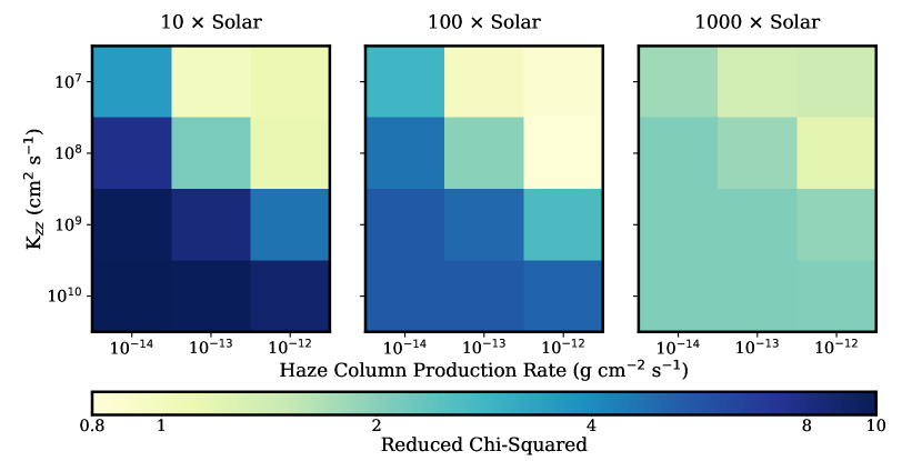
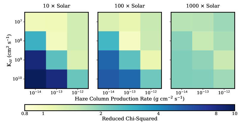
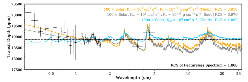
Figure 11 shows the RCS values for the full grid of tholin and soot haze models. In both cases, the best-performing run (lowest RCS) has an atmospheric metallicity of 100 solar and a moderate rate of vertical mixing ( cm2 s-1). For tholins, the observations are best matched when assuming a haze production rate of g cm-2 s-1, whereas for soot, a lower production rate of g cm-2 s-1 is preferred, since soots are more absorbing than hazes at the wavelengths of interest (Adams et al. 2019). The model transmission spectra derived from the best-fitting condensate cloud, tholin, and soot models are shown in Figure 12. Both of the photochemical haze models match the full set of observations and have RCS values below 1. Meanwhile, the lowest-RCS condensate cloud model performs more poorly than even a featureless flat spectrum. When comparing the soot and tholin spectra, the only salient distinguishing feature is at 6.5 m, where the tholin spectrum displays an additional absorption possibly attributable to double-bonded carbon atoms, double-bonded carbon and nitrogen atoms, and single-bonded amine groups (Imanaka et al. 2004; Gautier et al. 2012).
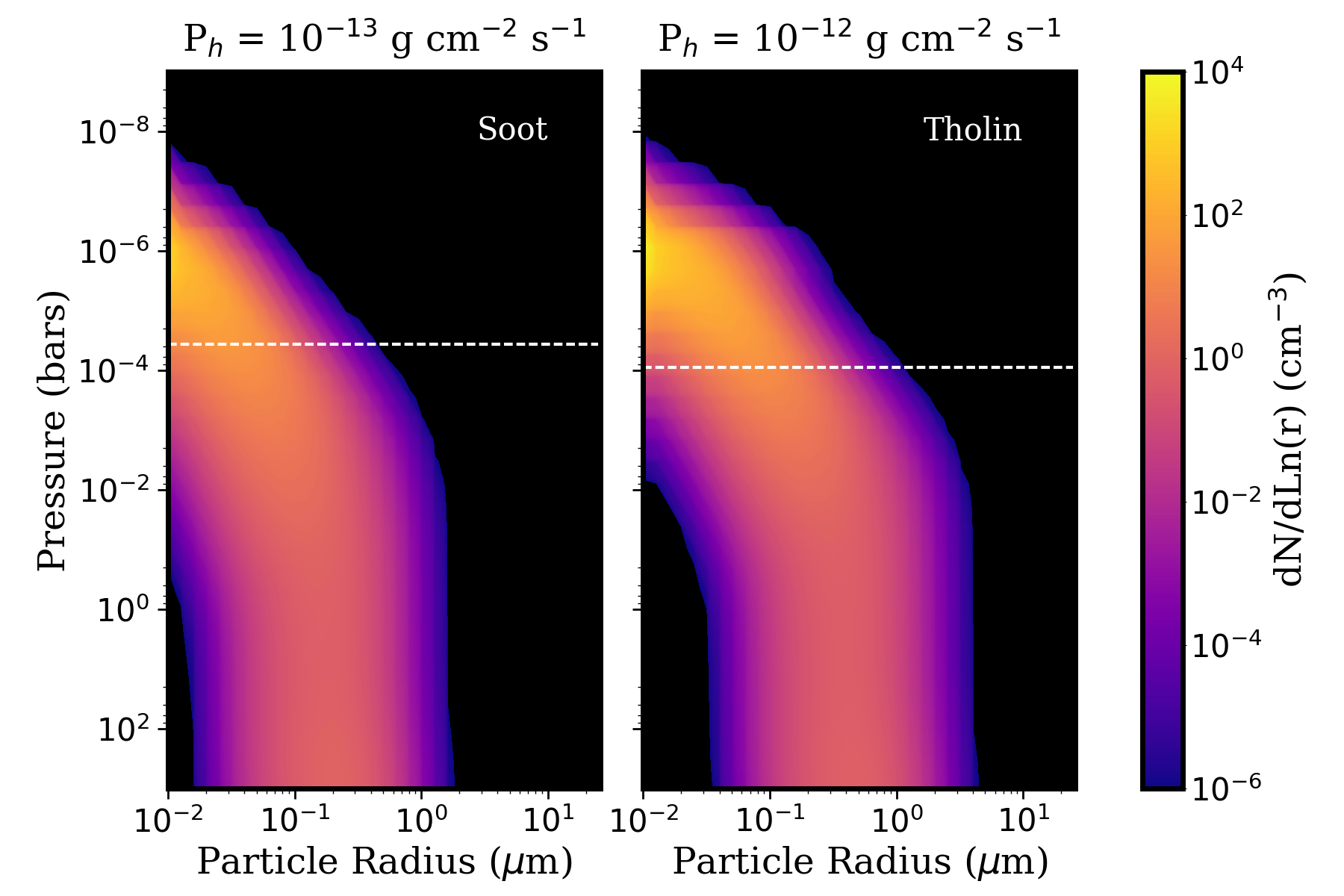
The size and vertical distributions of the haze particles for the soot and tholin models are shown in Figure 13. The color coding indicates the number density of particles per logarithmic radius bin. For both cases, the haze distribution is dominated by submicron particles, particularly at the lowest pressure levels (below 0.1 mbar), consistent with the observed Rayleigh scattering slope in visible wavelengths. The horizontal dashed lines denote the highest pressure probed by our observations (i.e., optical depth of unity in transmission). Notably, the modeled particle size distributions and the opacity pressure levels are in agreement with the corresponding values and inferred from the SCARLET retrieval (Table 6) to within the uncertainties. The demonstrated agreement between the retrieval and the CARMA results serves as an illustrative example of the increasing explanatory power of current aerosol models that incorporate detailed microphysical calculations and account for the opacity contributions from photochemical hazes.
6. Constraints from secondary eclipse measurements
The secondary eclipse measurements offer an independent look at the atmosphere of HAT-P-12b. While the transmission spectrum directly probes the day–night terminators, the secondary eclipse depths indicate the total outgoing flux from the dayside hemisphere relative to the star’s flux. In Section 3.3, we calculated depths of and at 3.6 and 4.5 m, respectively.
From these values, we can estimate the blackbody brightness temperature of the dayside hemisphere. We account for the uncertainties in the stellar parameters by deriving empirical analytical functions for the integrated stellar flux in the Spitzer bandpasses. This is done by fitting a polynomial in (, [M/H], ) to the calculated stellar flux for a grid of ATLAS models (Castelli & Kurucz 2004) spanning the ranges K, , and . We then computed the posterior distribution of the dayside brightness temperature using a Monte Carlo sampling method, given priors on the stellar properties from Hartman et al. (2009).
We obtain brightness temperature estimates of K at 3.6 m and K at 4.5 m. We also find that both eclipse depths are consistent with a single blackbody temperature of K. This estimate is consistent at the level with the terminator temperature of K previously derived from an analysis of the HST STIS transmission spectrum when assuming Rayleigh scattering (Sing et al. 2016). The predicted dayside equilibrium temperature of HAT-P-12b assuming zero albedo is 1150 K if incident energy is reradiated from the dayside only and 970 K if the planet reradiates the absorbed energy uniformly over the entire surface. The relatively low calculated dayside temperature indicates very efficient day–night recirculation of incident energy and possibly a nonzero albedo.
The Spitzer secondary eclipse depths can also provide constraints on atmospheric metallicity. Specifically, the ratio between the 3.6 and 4.5 m depths varies systematically with metallicity. From the bottom left panel of Figure 7, we see the comparison between the measured depths and model spectra generated by SCARLET. The constraints provided by the Spitzer secondary eclipse depths in the combined transmission and emission spectra retrieval are weak due to the low signal-to-noise of the planetary flux detection as well as the low wavelength resolution of the two broadband points. Examining the model emission spectra, we can see diagnostic features in the 3–5 m region that could be adequately probed with even modest wavelength resolution (). Near-future instruments, such as NIRSpec on the James Webb Space Telescope (JWST), will enable detailed studies of planetary emission spectra spanning the thermal infrared, opening up a new domain for exoplanet atmospheric characterization.
7. Conclusions
We have presented eight transit observations of the warm sub-Saturn HAT-P-12b obtained from HST and Spitzer. The resulting transmission spectrum from a joint analysis of all transit light curves covers the optical and near-infrared wavelength range from 0.3 to 5.0 m. We obtain precise, updated estimates for the orbital parameters of the system.
The main features of the transmission spectrum are a weak water vapor absorption feature at 1.4 m and a prominent Rayleigh scattering slope throughout the visible wavelength range with no detected alkali absorption peaks. These features indicate significant cloud opacity in the atmosphere of HAT-P-12b, with a strong contribution from small-particle scattering in the upper atmosphere. The detection of Rayleigh scattering in the transmission spectrum and the low stellar activity of the host star make HAT-P-12b an important test case for evaluating the relationship between optical scattering slopes and stellar activity.
We have complemented our analysis of the transmission spectrum with new fits of secondary eclipse light curves in the 3.6 and 4.5 m Spitzer bandpasses, from which we derive the depths and , respectively. The dayside atmosphere is consistent with a single blackbody temperature of K and efficient day–night heat recirculation.
Through a multifaceted approach combining atmospheric retrievals from SCARLET using both transmission and emission spectra with the results of the aerosol microphysics model CARMA, we find that the atmosphere of HAT-P-12b has a near-solar C/O ratio of and an atmospheric metallicity that broadly spans the range between several tens and a few hundred times solar. While condensate cloud models produce particles that are too large to reproduce the observed Rayleigh scattering slope, models incorporating photochemical hazes consisting of tholins or soot readily generate submicron particles in the upper atmosphere and match the full range of observations. The aerosol modeling indicates moderate vertical mixing (eddy diffusion coefficient cm2 s-1) and opacity pressure levels around 0.1 mbar, consistent with the results of the retrievals.
HAT-P-12b fits within the growing population of well-characterized cooler exoplanets that show evidence for photochemical hazes. The temperature range spanned by these planets allows for the formation of an enormous diversity of condensate species (e.g., Sing et al. 2016). The importance of clouds and hazes in interpreting observed transmission spectra and their wide-ranging effects on atmospheric chemistry and dynamics illustrates the need for continued refinement in our understanding of the myriad physical and chemical processes that govern the formation and distribution of condensates in exoplanetary atmospheres. While current state-of-the-art cloud and haze models are becoming more sophisticated and capable of describing observations of individual exoplanets and observed trends in exoplanet cloudiness, there remain significant gaps in our knowledge of the detailed microphysics of ab initio aerosol formation and the effects of secondary processes such as vertical mixing.
Our work also underscores the importance of increased spectral resolution in amplifying the explanatory power of both transmission and emission spectroscopy. The broadband Spitzer photometry at 3.6 and 4.5 m has provided weak complementary constraints on the more discerning transmission spectra at shorter wavelengths. However, with even moderately increased spectral resolution in the 2–5 m region, we can obtain much more precise estimates of atmospheric metallicity and C/O ratio and probe the absorption and emission features of a wide range of major atmospheric species. The capabilities of upcoming space-based telescopes such as JWST in this regard will usher in a new era of exoplanet atmospheric characterization.
This work is based on observations with the NASA/ESA Hubble Space Telescope, obtained at the Space Telescope Science Institute (STScI) operated by AURA, Inc. This work is also based in part on observations made with the Spitzer Space Telescope, which is operated by the Jet Propulsion Laboratory, California Institute of Technology, under a contract with NASA. The research leading to these results has received funding from the European Research Council under the European Union’s Seventh Framework Program (FP7/2007-2013)/ERC grant agreement No. 336792. Support for this work was also provided by NASA/STScI through grants linked to the HST-GO-12473 and HST-GO-14767 programs. I.W. and P.G. are supported by Heising-Simons Foundation 51 Pegasi b postdoctoral fellowships. H.A.K. acknowledges support from the Sloan Foundation.
References
- (1)
- Ackerman & Marley (2001) Ackerman, A., & Marley, M. 2001, ApJ, 556, 872
- Adams et al. (2019) Adams, D., Gao, P., de Pater, I., & Morley, C. 2019, ApJ, 874, 61
- Alexoudi et al. (2018) Alexoudi, X., Mallonn, M., von Essen, C. 2018, A&A, 620, A142
- Barstow et al. (2017) Barstow, J. K., Aigrain, S., Irvin, P. G. J., & Sing, D. K. 2017, ApJ 834, 50
- Barth & Toon (2006) Barth, E. L., & Toon, O. B. 2006, Icar, 182, 230
- Bean et al. (2018) Bean, J. L., Stevenson, K. B., Batalha, N. M., et al. 2018, PASP, 130, 114402
- Benneke & Seager (2012) Benneke, B., & Seager, S. 2012, ApJ, 753, 100
- Benneke & Seager (2013) — 2013, ApJ, 778, 153
- Benneke (2015) Benneke, B. 2015, arXiv:1504.07655
- Benneke et al. (2017) Benneke, B., Werner, M., Petigura, E., et al. 2017, ApJ, 834, 187
- Benneke et al. (2019) Benneke, B., Knutson, H. A., Lothringer, J., et al. 2019, NatAs, 3, 813
- Berta et al. (2012) Berta, Z. K., Charbonneau, D., Désert, J.-M., et al. 2012, ApJ, 747, 35
- Caldas et al. (2019) Caldas, A., Leconte, J., Selsis, F., et al. 2019, A&A, 623, A161
- Castelli & Kurucz (2004) Castelli, F., & Kurucz, R. L. 2004, arXiv:astro-ph/0405087
- Charnay et al. (2018) Charnay, B., Bézard, B., Baudino, J.-L., et al. 2018, ApJ, 854, 172
- Colaprete et al. (1999) Colaprete, A., Toon, O. B., & Magalhães, J. A. 1999, JGR, 104, 9043
- Crouzet et al. (2014) Crouzet, N., McCullough, P., Deming, D., & Madhusudhan, N. 2014, ApJ, 791, 55
- Deming et al. (2015) Deming, D., Knutson, H. A., Kammer, J., et al. 2015, ApJ, 805, 132
- Deming & Seager (2017) Deming, D., & Seager, S. 2017, JGRE, 122, 53
- Deming et al. (2013) Deming, D., Wilkins, A., McCullough, P., et al. 2013, ApJ, 774, 95
- Demory et al. (2013) Demory, B.-O., de Wit, J., Lewis, N., et al. 2013, ApJL, 776, L25
- Evans et al. (2016) Evans, T. M., Sing, D. K., Wakeford, H. R., et al. 2016, ApJL, 822, L4
- Fleury et al. (2018) Fleury, B., Gudipati, M. S., Henderson, B. L., & Swain, M. 2018, ApJ, 871, 158
- Foreman-Mackey et al. (2013) Foreman-Mackey, D., Hogg, D. W., Lang, D., & Goodman, J. 2013, PASP, 125, 306
- Fortney (2005) Fortney, J. J. 2005, MNRAS, 364, 649
- Fortney et al. (2013) Fortney, J. J., Mordasini, C., Nettelmann, N., et al. 2013, ApJ, 775, 80
- Fortney et al. (2010) Fortney, J. J., Shabram, M., Showman, A. P., et al. 2010, ApJ, 709, 1396
- Fraine et al. (2014) Fraine, J., Deming, D., Benneke, B., et al. 2014, Natur, 513, 526
- Gao & Benneke (2018) Gao, P., & Benneke, B. 2018, ApJ, 863, 165
- Gao et al. (2017) Gao, P., Fan, S., Wong, M., et al. 2017, Icar, 287, 116
- Gao et al. (2018) Gao, P., Marley, M. S., & Ackerman, A. A. 2018, ApJ, 855, 86
- Gao et al. (2014) Gao, P., Zhang, X., Crisp, D., Bardeen, C. G., & Yung, Y. L. 2014, Icar, 231, 83
- Gautier et al. (2012) Gautier, T., Carrasco, N., Mahjoub, A., et al. 2012, Icar, 221, 320
- Hartman et al. (2009) Hartman, J. D., Bakos, G. Á., Torres, G., et al. 2009, ApJ, 706, 785
- He et al. (2018) He, C., Hörst, S. M., Lewis, N. K., et al. 2018, AJ, 156, 38
- Helling (2019) Helling, Ch. 2019, AREPS, 47, 583
- Helling et al. (2008) Helling, Ch., Ackerman, A., Allard, F., et al. 2008, MNRAS, 391, 1854
- Helling et al. (2019a) Helling, Ch., Gourbin, P., Woitke, P., & Parmentier, V. 2019, A&A, 626, A133
- Helling et al. (2019b) Helling, Ch., Iro, N., Corrales, L., et al. 2019, A&A, 631, A79
- Helling et al. (2016) Helling, Ch., Lee, G., Dobbs-Dixon, I., et al. 2016, MNRAS, 460, 855
- Heng & Showman (2015) Heng, K., & Showman, A. P. 2015, AREPS, 43, 509
- Hörst et al. (2018) Hörst, S. M., He, C., Lewis, N. K., et al. 2018, NatAs, 2, 303
- Husser et al. (2013) Husser, T-O., Wende-von Berg, S., Dreizler, S., et al. 2013, A&A, 553, A6
- Imanaka et al. (2004) Imanaka, H., Khare, B. N., Elsila, J. E., et al. 2004, Icar, 168, 344
- James et al. (1997) James, E. P., Toon, O. B., & Schubert, G. 1997, Icar, 129, 147
- Kataria et al. (2016) Kataria, T., Sing, D. K., Lewis, N. K., et al. 2016, ApJ, 821, 9
- Kawashima & Ikoma (2018) Kawashima, Y., & Ikoma, M. 2018, ApJ, 853, 7
- Knutson et al. (2014) Knutson, H. A., Dragomir, D., Kreidberg, L., et al. 2014, ApJ, 794, 155
- Knutson et al. (2010) Knutson, H. A., Howard, A. W., & Isaacson, H. 2010, ApJ, 720, 1569
- Knutson et al. (2012) Knutson, H. A., Lewis, N. K., Fortney, J. J., et al. 2012, ApJ, 754, 22
- Kreidberg (2015) Kreidberg, L. 2015, PASP, 127, 1161
- Kreidberg et al. (2014) Kreidberg, L., Bean, J. L., Désert, J. M., et al. 2014, Natur, 505, 69
- Kreidberg et al. (2015) Kreidberg, L., Line, M. R., Bean, J. L., et al. 2015, ApJ, 814, 66
- Kuntschner et al. (2009) Kuntscher, H., Bushouse, H., Kümmel, M., & Walsh, J. R. 2009, WFC3 SMOV proposal 11552: Calibration of the G141 grism, Tech. Rep. WFC3-2009-17
- Kuntschner et al. (2011) Kuntscher, H., Kümmel, M., Walsh, J. R., & Bushouse, H. 2011, Revised Flux Calibration of the WFC3 G102 and G141 grisms, Tech. Rep. WFC3-2011-05
- Lavvas & Koskinen (2017) Lavvas, P., & Koskinen, T. 2017, ApJ, 847, 32
- Lee et al. (2016) Lee, G., Dobbs-Dixon, I., Helling, Ch., Bognar, K., & Woitke, P. 2016, A&A, 594, A48
- Lee et al. (2018) Lee, G. K. H., Blecic, J., & Helling, Ch. 2018, A&A, 614, A126
- Lewis et al. (2013) Lewis, N. K., Knutson, H. A., Showman, A. P., et al. 2013, ApJ, 766, 95
- Line et al. (2013) Line, M. R., Knutson, H., Deming, D., Wilkins, A., & Desert, J. M. 2013, ApJ, 778, 183
- Line & Parmentier (2016) Line, M. R., & Parmentier, V. 2016, ApJ, 820, 78
- Line et al. (2011) Line, M. R., Vasisht, G., Chen, P., Angerhausen, D., & Yung, Y. L. 2011, ApJ, 738, 32
- Lines et al. (2018a) Lines, S., Manners, J., Mayne, N. J., et al. 2018, MNRAS, 481, 194
- Lines et al. (2018b) Lines, S., Mayne, N. J., Boutle, I. A. et al. 2018, A&A, 615, 97
- Lodders & Fegley (2002) Lodders, K., & Fegley, B. 2002, Icar, 155, 393
- Lunine et al. (1989) Lunine, J. I., Hubbard, W. B., Burrows, A., Wang, Y.-P., & Garlow, K. 1989, ApJ, 338, 314
- Madhusudhan et al. (2016) Madhusudhan, N., Bitsch, B., Johansen, A., & Eriksson, L. 2016, MNRAS, 469, 4102
- Madhusudhan et al. (2014) Madhusudhan, N., Knutson, H., Fortney, J. J., & Barman, T. 2014, in Protostars and Protoplanets IV, ed. H. Beuther, R. S. Klessen, C. P. Dullemond, & T. Henning (Tucson, AZ: University of Arizona Press), 739
- Mallonn et al. (2015) Mallonn, M., Nascimbeni, V., Weingrill, J., et al. 2015, A&A, 583, A138
- Mancini et al. (2018) Mancini, L., Esposito, M., Covino, E., et al. 2018, A&A, 613, A41
- Marley et al. (2013) Marley, M. S., Ackerman, A. S., Cuzzi, J. N., & Kitzmann, D. 2013, in Comparative Climatology of Terrestrial Planets, ed. S. J. Mackwell, A. A. Simon-Miller, J. W. Harder, & M. A., Bullock (Tucson, AZ: University of Arizona Press), 367
- Marley et al. (1999) Marley, M. S., Gelino, C., Stephens, D., Lunine, J. I., & Freedman, R. 1999, ApJ, 513, 879
- Mordasini et al. (2012) Mordasini, C., Alibert, Y., Benz, W., Klahr, H., & Henning, T. 2012, A&A, 541, A97
- Morley et al. (2012) Morley, C. V., Fortney, J. J., Marley, M. S., et al. 2012, ApJ, 756, 172
- Morley et al. (2015) Morley, C. V., Fortney, J. J., Marley, M. S., et al. 2015, ApJ, 815, 110
- Morley et al. (2017) Morley, C. V., Knutson, H., Line, M., et al. 2017, AJ, 153, 86
- Moses et al. (2011) Moses, J. I., Visscher, C., Fortney, J. J., et al. 2011, ApJ, 737, 15
- Nikolov et al. (2015) Nikolov, N., Sing, D. K., Burrows, A. S., et al. 2015, MNRAS, 447, 463
- Nikolov et al. (2014) Nikolov, N., Sing, D. K., Pont, F., et al. 2014, MNRAS, 437, 46
- Ohno & Okuzumi (2017) Ohno, K., & Okuzumi, S. 2017, ApJ, 835, 261
- Parmentier & Guillot (2014) Parmentier, V., & Guillot, T. 2014, A&A, 562, A133
- Parmentier et al. (2013) Parmentier, V., Showman, A. P., & Lian, Y. 2013, A&A, 558, A91
- Parviainen & Aigrain (2015) Parviainen, H., & Aigrain, S. 2015, MNRAS, 453, 3821
- Pollack et al. (1996) Pollack, J. B., Hubickyj, O., Bodenheimer, P., et al. 1996, Icar, 124, 62
- Pont et al. (2008) Pont, F., Knutson, H. A., Gilliland, R. L., Moutou, C., & Charbonneau, D. 2008, MNRAS, 385, 109
- Posch et al. (2003) Posch, T., Kerschbaum, F., Fabian, D., et al. 2003, ApJS, 149, 437
- Powell et al. (2019) Powell, D., Louden, T., Kreidberg, L., et al. 2019, ApJ, 887, 170
- Powell et al. (2018) Powell, D., Zhang, X., Gao, P., & Parmentier, V. 2018, ApJ, 860, 18
- Pruppacher & Klett (1978) Pruppacher, H. R., & Klett, J. D. 1978, Microphysics of Clouds and Precipitation (Springer Netherlands)
- Rackham et al. (2018) Rackham, B. V., Apai, D., & Giampapa, M. S. 2018, ApJ, 853, 122
- Rothman et al. (2010) Rothman, L. S., Gordon, I. E., Barber, R. J., et al. 2010, JQSRT, 111, 2139
- Tennyson et al. (2012) Tennyson, J., & Yurchenko, S. N. 2012, MNRAS, 425, 21,
- Schlawin et al. (2018) Schlawin, E., Greene, T. P., Line, M., Fortney, J. J., & Rieke, M. 2018, AJ, 156, 40
- Showman et al. (2010) Showman, A. P., Cho, J. Y.-K., & Menou, K. 2010, in Exoplanets, ed. S. Seager (Tucson, AZ: University of Arizona Press), 471
- Shporer & Hu (2015) Shporer, A., & Hu, R. 2015, AJ, 150, 112
- Sing (2010) Sing, D. K. 2010, A&A, 510, A21
- Sing et al. (2016) Sing, D. K., Fortney, J. J., Nikolov, N., et al. 2016, Natur, 529, 59
- Sing et al. (2008) Sing, D. K., Vidal-Madjar, A., Désert, J.-M., Lecavelier des Etangs, A., & Ballester, G. 2008, ApJ, 686, 658
- Sing et al. (2015) Sing, D. K., Wakeford, H. R., Showman, A. P., et al. 2015, MNRAS, 446, 2428
- Spake et al. (2019) Spake, J. J., Sing, D. K., Wakeford, H. R., et al. 2019, MNRAS, in review (arXiv:1911.08859)
- Thorngren & Fortney (2019) Thorngren, D. P., & Fortney, J. J. 2019, ApJL, 874, L31
- Thorngren et al. (2016) Thorngern, D. P., Fortney, J. J., Murray-Clay, R. A., & Lopez, E. D. 2016, ApJ, 831, 64
- Todorov et al. (2013) Todorov, K. O., Deming, D., Knutson, H. A., et al. 2013, ApJ, 770, 102
- Toon et al. (1992) Toon, O. B., McKay, C. P., Griffith, C. A., & Turco, R. P. 1992, Icar, 95, 24
- Toon et al. (1979) Toon, O. B., Turco, R. P., Hamill, P., Kiang, C. S., & Whitten, R. C. 1979, JAtS, 36, 718
- Tsiaras et al. (2016) Tsiaras, A., Waldmann, I. P., Rocchetto, M., et al. 2016, ApJ, 832, 202
- Tsiaras et al. (2018) Tsiaras, A., Waldmann, I. P., Zingales, T., et al. 2018, AJ, 155, 156
- Turco et al. (1979) Turco, R. P., Hamill, P., Toon, O. B., Whitten, R. C., & Kiang, C. S. 1979, JAtS, 36, 699
- Venot et al. (2015) Venot, O., Hébrard, E., Agúndez, M., Decin, L., & Bounaceur, R. 2015, A&A, 577, A33
- Visscher et al. (2006) Visscher, C., Lodders, K., & Fegley, B. Jr. 2006, ApJ, 648, 1181
- Visscher et al. (2010) Visscher, C., Lodders, K., & Fegley, B. Jr. 2010, ApJ, 716, 1060
- Wakeford & Sing (2015) Wakeford, H. R., & Sing, D. K. 2015, A&A, 573, A122
- Wakeford et al. (2017) Wakeford, H. R., Visscher, C., Lewis, N. K., et al. 2017, MNRAS, 464, 4247
- Wilkins et al. (2014) Wilkins, A. N., Deming, D., Madhusudhan, N., et al. 2014, ApJ, 783, 113
- Wilson & Militzer (2012) Wilson, H. F., & Militzer, B. 2012, ApJ, 745, 54
- Wong et al. (2016) Wong, I., Knutson, H. A., Kataria, T., et al. 2016, ApJ, 823, 122
- Wong et al. (2015) Wong, I., Knutson, H. A., Lewis, N. K., et al. 2015, ApJ, 811, 122
- Woitke & Helling (2003) Woitke, P, & Helling, Ch. 2003, A&A, 399, 297
- Woitke et al. (2020) Woitke, P., Helling, Ch., & Gunn, O. 2020, A&A, 623, A23
- Woitke et al. (2018) Woitke, P., Helling, Ch., Hunter, G. H., et al. 2018, A&A, 614, A1
- Zahnle et al. (2009b) Zahnle, K., Marley, M. S., Freedman, R. S., Lodders, K., & Fortney, J. J. 2009, ApJL, 701, L20
- Zeidler et al. (2011) Zeidler, S., Posch, T., Mutschke, H., Richter, H. & Wehrhan, O. 2011, A&A, 526, A68
- Zhang & Showman (2018) Zhang, X., & Showman, A. P. 2018, ApJ, 866, 1
Appendix A HST Light Curves
The following plots show the spectroscopic light curves for the six HST WFC3 and STIS transit observations. The left panel shows the light curves for each of the wavelength bins, corrected for instrumental systematics and arranged top to bottom in the order listed in Table 4. The best-fit transit light curves are overplotted in black. The right panel shows the corresponding residuals in parts per thousand (ppt). The error bars on all data points are set to the best-fit photometric noise parameter.
![[Uncaptioned image]](/html/2004.03551/assets/x14.png)
![[Uncaptioned image]](/html/2004.03551/assets/x15.png)
![[Uncaptioned image]](/html/2004.03551/assets/x16.png)
![[Uncaptioned image]](/html/2004.03551/assets/x17.png)
![[Uncaptioned image]](/html/2004.03551/assets/x18.png)
![[Uncaptioned image]](/html/2004.03551/assets/x19.png)
Appendix B Cloud and haze modeling with CARMA
CARMA was initially developed to investigate aerosol processes on Earth (Toon et al. 1979; Turco et al. 1979), and has since been adapted to various solar system bodies (Toon et al. 1992; James et al. 1997; Colaprete et al. 1999; Barth & Toon 2006; Gao et al. 2014, 2017) and exoplanets (Gao & Benneke 2018; Powell et al. 2018, 2019; Adams et al. 2019). Here we use the exoplanet version of CARMA, which has the ability to model clouds composed of a variety of species predicted by equilibrium chemistry and kinetic cloud formation models, including KCl, ZnS, Na2S, MnS, Cr, Mg2SiO4, Fe, TiO2, and Al2O3 (see, for example, the review in Marley et al. 2013). We refer the reader to Gao & Benneke (2018) and Powell et al. (2019) for the relevant material properties of the condensates and the formation pathways we consider. Briefly, we consider homogeneous nucleation for species that can undergo direct phase change (TiO2, Fe, Cr, and KCl) and heterogeneous nucleation for species that form via thermochemical reactions, represented in the gas phase by their limiting species (Al2O3: Al, Mg2SiO4: Mg, MnS: Mn, Na2S: Na, ZnS: Zn; see, for example, Visscher et al. 2006, Visscher et al. 2010, and Morley et al. 2012). Here TiO2 is chosen to be the condensation nuclei of Al2O3, Mg2SiO4, MnS, and Na2S due to its low energy barrier to homogeneous nucleation (e.g., Lee et al. 2018), while KCl acts as the condensation nuclei to ZnS, as they both form at lower temperatures than the other condensates. Here Fe and Cr are also allowed to heterogeneously nucleate on TiO2. The resulting cloud particles are either pure, in the case of the homogeneously nucleated particles, or a core surrounded by a mantle, in the case of the heterogeneously nucleated particles. This is a simplification of the mixed-grains formalism of other kinetic cloud models (e.g., Helling et al. 2016; Lee et al. 2016; Lines et al. 2018b). Cloud particles of different compositions do not interact, and their size distributions are computed independently of each other, except in the case of condensation nuclei and mantling species; i.e. formation of the latter depletes the former.
Each cloud simulation begins with a background H2/He atmosphere devoid of cloud particles, with condensate vapor only at the deepest atmospheric level. We use GGchem (Woitke et al. 2018) to set the initial mixing ratio of each condensate species at this lower boundary. As the simulation advances, all condensate vapors are mixed upward via eddy diffusion and parameterized by the eddy diffusion coefficient , until they either become well mixed in the atmosphere or achieve supersaturation. Particle nucleation and condensation may then occur, provided that the supersaturation is sufficiently large to overcome the nucleation energy barriers of the various condensate species. Cloud particle formation depletes the condensate vapors until their resupply by eddy diffusion from depth is sufficient to balance. We do not explicitly consider any gas chemistry in our modeling. Growth of cloud particles by coagulation and vertical transport of cloud particles proceed until a steady state is reached.
CARMA also models coagulation and vertical transport of photochemical hazes, following the methodology developed in Gao et al. (2017) and Adams et al. (2019). The detailed chemical pathways and formation efficiencies of exoplanet hazes are much more complex and less understood than those predicted for condensation clouds (Fleury et al. 2018; He et al. 2018; Hörst et al. 2018), and CARMA does not explicitly model the production of aerosol particles. Instead, we choose to model haze production generically by setting the haze production rate as a free parameter. We assume spherical haze particles with a mass density of 1 g cm-3 and a minimum radius of 10 nm; it has been shown that the minimum particle radius does not strongly affect the optical depth at equilibrium (e.g., Adams et al. 2019). We do not consider condensation when modeling hazes.
Haze simulations also begin with a background H2/He atmosphere devoid of aerosols. As the simulation advances, 10 nm haze particles are produced at high altitudes, after which they can grow by coagulation and are transported into the deep atmosphere by sedimentation and eddy diffusion. Haze particles are assumed to evaporate at the lower boundary of the model, though it does not impact the resulting transmission spectra, since the lower boundary is set at pressures 10 bar.
To generate predicted transmission spectra from the forward-modeled aerosol distributions, we first use the pymiecoated tool to compute the extinction efficiency, single scattering albedo, and asymmetry factor of the aerosol particles. The refractive indices for the various aerosol species are compiled from Posch et al. (2003), Zeidler et al. (2011), Morley et al. (2012), Wakeford & Sing (2015), and Lavvas & Koskinen (2017). We then use a standard 1D radiative transfer model to produce the transmission spectra (e.g., Fortney et al. 2010). These spectra are subsequently binned to the resolution of the observations, and the base planet radius is shifted to best fit the observed transmission spectrum. We compute the RCS goodness-of-fit metric to choose the best-performing model runs.