Instabilities in Multi-Asset and Multi-Agent
Market Impact Games

Abstract

We consider the general problem of a set of agents trading a portfolio of assets in the presence of transient price impact and additional quadratic transaction costs and we study, with analytical and numerical methods, the resulting Nash equilibria. Extending significantly the framework of citeschied2018market and citeluo_schied, who considered the single asset case, we prove the existence and uniqueness of the corresponding Nash equilibria for the related mean-variance optimization problem. We then focus our attention on the conditions on the model parameters making the trading profile of the agents at equilibrium, and as a consequence the price trajectory, wildly oscillating and the market unstable. While citeschied2018market and citeluo_schied highlighted the importance of the value of transaction cost in determining the transition between a stable and an unstable phase, we show that also the scaling of market impact with the number of agents $J$ and the number of assets $M$ determines the asymptotic stability (in $J$ and $M$) of markets.

Keywords: Market impact; Game theory and Nash equilibria; Transaction costs; Market microstructure; High Frequency Trading; Cross-Impact.

Statements and Declarations: Not applicable.

1 Introduction

Instabilities in financial markets have always attracted the attention of researchers, policy makers and practitioners in the financial industry because of the role that financial crises have on the real economy. Despite this, a clear understanding of the sources of financial instabilities is still missing, in part probably because several origins exist and they are different at different time scales. The recent automation of the trading activity has raised many concerns about market instabilities occurring at short time scales (e.g. intraday), also because of the attention triggered by the Flash Crash of May 6th, 2010 (citeKirilenko) and the numerous other similar intraday instabilities observed in more recent years (citeJohnson, citegolub, citeCalcagnile, citeBrogaard), such as the Treasury bond flash crash of October 15th, 2014. The role of High Frequency Traders (HFTs), Algo Trading, and market fragmentation in causing these events has been vigorously debated, both theoretically and empirically (citegolub, citeBrogaard).

One of the puzzling characteristics of market instabilities is that a large fraction of them appear to be endogenously generated, i.e. it is often very difficult to find an exogenous event (e.g. a news) which can be considered at the origin of the instability (citeCutler, Fair, Joulin). Liquidity plays a crucial role in explaining these events. Markets are, in fact, far from being perfectly elastic and any order or trade causes prices to move, which in turn leads to a cost (termed slippage) for the investor. The relation between orders and price is called market impact. In order to minimize market impact cost, when executing a large volume it is optimal for the investor to split the order in smaller parts which are executed incrementally over the day or even across multiple days. One of the origins of market impact cost is predatory trading (citeBrunnermeier, Carlin): the knowledge that a trader is purchasing progressively a certain amount of assets can be used to make profit by buying at the beginning and selling at the end of the trader’s execution. Part of the core strategy of HFTs is exactly predatory trading. Now, the combined effect on price of the trading of the predator and of the prey can lead to large price oscillations and market instabilities. In any case, it is clear that the price dynamics is the result of the (dynamical) equilibrium between the activity of two or more agents simultaneously trading.

This equilibrium can be studied by modeling the above setting as a market impact game (citeCarlin , citeschoneborn2008trade, citeMoallemi, citeLachapelle, schied2018market, Strehle, strehle2017single). In a nutshell, in a market impact game, two traders want to trade the same asset in the same time interval. While trading, each agent modifies the price because of market impact, thus when two (or more) traders are simultaneously present, the optimal execution schedule of a trader should take into account the simultaneous presence of the other trader(s). As customary in these situations, the approach is to find the Nash equilibrium, which in general depends on the market impact model.

Market impact games are a perfect modeling setting to study endogenously generated market instabilities. A major step in this direction has been recently made by citeschied2018market. By using the transient impact model of citeBouchaud, BFL plus a quadratic temporary impact cost (which can alternatively be interpreted as a quadratic transaction cost, see below), they have recently considered a simple setting with two identical agents liquidating a single asset and derived the Nash equilibrium. Interestingly, they also derived analytically the conditions on the transaction cost under which the Nash equilibrium displays huge oscillations of the trading volume and, as a consequence, of the price, thus leading to market instabilities. Specifically, they proved the existence of a sharp transition between stable and unstable markets at a specific value of the transaction cost parameter.

Although the paper of Schied and Zhang highlights a key mechanism leading to market instability, several important aspects are left unanswered. First, market instabilities rarely involve only one asset and, as observed for example during the Flash Crash, a cascade of instabilities affects very rapidly a large set of assets or the entire market (citeCFTC). This is due to the fact that optimal execution strategies often involve a portfolio of assets rather than a single one (see, e.g. citeGerry). Commonality of liquidity across assets (citeChordia and cross-impact effects (citealfonsi2016multivariate, citeschneider2018cross) makes the trading on one asset triggers price changes on other assets. Furthermore, citecespa2014 show that a drop in liquidity in one asset can propagate in another asset, causing a market liquidity crash. Thus, it is natural to ask: is a large market more or less prone to market instabilities? How does the structure of cross-impact and therefore of liquidity commonality affect the market stability? A second class of open questions regards instead the market participants. Do the presence of more agents simultaneously trading one asset tends to stabilize the market? While the solution of Schied and Zhang considers only two traders, it is important to know whether having more agents is beneficial or detrimental to market stability. For example, regulators and exchanges could implement mechanisms to favor or disincentive participation during turbulent periods. Answering this question requires solving the impact game with a generic number of agents and it is discussed in the single asset case in citeluo_schied.

In this paper we extend considerably the setting of Schied and Zhang by answering the above research questions. Specifically, starting from citeluo_schied, we consider (i) the case when agents trade multiple assets simultaneously and cross market impact is present and we provide explicit representations of related Nash equilibria; (ii) after studying how trading conditions may be affected by the cross impact, we derive theoretical results on market stability for the $J=2$ agents by showing how it is related to cross-impact effects; (iii) we study numerically market stability in the general case and we extend a previous result and conjecture of citeluo_schied in the multi-asset case.

It is important to notice that in market impact games, market impact is taken as exogenously given. Market microstructure literature has extensively discussed its endogenous nature since the seminal work of citeKyle. Theoretical and empirically studies have investigated and provided evidence of how market impact might depend on number of agents and of traded assets, e.g., citeBagnoli, citebenzaquen2017dissecting, citecoimpact, citegarcia2020multivariate. Therefore we will consider this dependence and show how the stability of markets in market impact games depends on the way impact scales with the number of agents and the number of assets. We find that, if market impact is independent from the number of agents and assets, larger and more crowded markets are more prone to market instability. However, if, as observed empirically and proposed theoretically, market impact suitably scales with these two quantities, stability can be recovered.

The paper is organized as follows. In Section 2 we recall some notation of the market impact games framework and the citeluo_schied model. We extend the basic model of citeluo_schied to the multi-asset case in Section 3, where we find the corresponding Nash equilibria for different objective functions. We analyse how the cross-impact modifies the trading profile and trading conditions in Section 4. Finally, in Section 5 we study how the cross-impact matrix affects the market stability and we present how impact must scale with the number of assets to preserve stability. Finally, in Section 6 we draw somw conclusions.

2 Market Impact Games

Consider two traders who want to trade simultaneously a certain number of shares, minimizing the trading cost. Since the trading of one agent affects the price, the other agent must take into account the presence of the former in optimizing her execution. This problem is termed market impact game and has received considerable attention in recent years (citeCarlin, schoneborn2008trade, Moallemi, Lachapelle, schied2018market, Strehle, strehle2017single). The seminal paper by Schied and Zhang, (citeschied2018market), considers a market impact game between two identical agents trading the same asset in a given time period.

When none of the two agents trade, the price dynamics is described by the so called unaffected price process $S_{t}^{0}$ which is a right-continuous martingale defined on a given probability space $(\Omega,(\mathscr{F}_{t})_{t\geq 0},\mathscr{F},\mathbb{P})$. A trader wants to unwind a given initial position with inventory $X$, where a positive (negative) inventory means a short (long) position, during a given trading time grid $\mathbb{T}=\{t_{0},t_{1},\ldots,t_{N}\},$ where $0=t_{0}<t_{1}<\cdots<t_{N}=T$ and following an admissible strategy, which is defined as follows:

Definition 2.1 (Admissible Strategy).

Given $\mathbb{T}$ and $X$, an admissible trading strategy for $\mathbb{T}$ and $X\in\mathbb{R}$ is a vector $\bm{\zeta}=(\zeta_{0},\zeta_{1},\ldots,\zeta_{N})$ of random variables such that:

• $\zeta_{k}\in\mathscr{F}_{t_{k}}\text{ and bounded},\ \forall k=0,1,\ldots,N.$

• $\zeta_{0}+\zeta_{1}+\cdots+\zeta_{N}=X$.

The random variable $\zeta_{k}$ represents the order flow at trading time $t_{k}$ where positive (negative) flow corresponds to a sell (buy) trade of volume $|\zeta_{k}|$. We denote with $X_{1}$ and $X_{2}$ the initial inventories of the two considered agents playing the game and with $\Xi=(\xi_{i,k})\in\mathbb{R}^{2\times(N+1)}$ the matrix of the respective strategies, where $\bm{\xi}_{1,\cdot}=\{\xi_{1,k}\}_{k\in\mathbb{T}}$ and $\bm{\xi}_{2,\cdot}=\{\xi_{2,k}\}_{k\in\mathbb{T}}$ are the strategies of trader $1$ and $2$, respectively. Traders are subject to fees and transaction costs and their objective is to minimize them by optimizing the execution. As customary in the literature, the costs are modeled by two components. The first one is a temporary impact component modeled by a quadratic term $\theta\xi_{j,k}^{2}$, respectively for trader $j$, which does not affect the price dynamics and depends on the immediate liquidity present in the order book. Notice that, as discussed in citeschied2018market, this term can also be interpreted as a quadratic transaction fee. Here we do not specify exactly what this term represents, sticking to the mathematical modeling approach of Schied and Zhang.

The second component is related to permanent impact and affects future price dynamics. Following citeschied2018market, we consider the celebrated transient impact model of citeBouchaud, BFL, which describes the price process $S_{t}^{\Xi}$ affected by the strategies $\Xi$ of the two traders, i.e.,

$$S_{t}^{\Xi}=S_{t}^{0}-\sum_{t_{k}<t}G(t-t_{k})(\xi_{1,k}+\xi_{2,k}),\quad\forall\ t\in\mathbb{T},$$

where $G:\mathbb{R}_{+}\to\mathbb{R}_{+}$ is the so called decay kernel, which describes the lagged price impact of a unit buy or sell order over time. Usual assumptions on $G$ are satisfied, i.e., it is convex, nonincreasing, nonconstant so that $t\mapsto G(|t|)$ is strictly positive definite in the sense of Bochner, see citeAlfonsi and citeschied2018market. Notice that by choosing a constant kernel $G$, one recovers the celebrated Almgren-Chriss model (citealmgren2001optimal).

The cost faced by each agent is the sum of the two components above. Specifically, let us denote with $\mathscr{X}(X,\mathbb{T})$ the set of admissible strategies for the initial inventory $X$ on a specified time grid $\mathbb{T}$, the cost functions are defined as:

Definition 2.2 (citeschied2018market).

Given $\mathbb{T}=\{t_{0},t_{1},\ldots,t_{N}\}$, $X_{1}$ and $X_{2}$. Let $(\varepsilon_{i})_{i=0,1,\ldots N}$ be an i.i.d. sequence of Bernoulli $\left(\frac{1}{2}\right)$-distributed random variables that are independent of $\sigma(\bigcup_{t\geq 0}\mathscr{F}_{t})$. Then the cost of $\bm{\xi}_{1,\cdot}\in\mathscr{X}(X_{1},\mathbb{T})$ given $\bm{\xi}_{2,\cdot}\in\mathscr{X}(X_{2},\mathbb{T})$ is defined as

$$C_{\mathbb{T}}(\bm{\xi}_{1,\cdot}|\bm{\xi}_{2,\cdot})=\sum_{k=0}^{N}\left(\frac{G(0)}{2}\xi_{1,k}^{2}-S_{t_{k}}^{\Xi}\xi_{1,k}+\varepsilon_{k}G(0)\xi_{1,k}\xi_{2,k}+\theta\xi_{1,k}^{2}\right)+X_{1}S_{0}^{0}$$

and the costs of $\bm{\xi}_{2,\cdot}$ given $\bm{\xi}_{1,\cdot}$ are

$$C_{\mathbb{T}}(\bm{\xi}_{2,\cdot}|\bm{\xi}_{1,\cdot})=\sum_{k=0}^{N}\left(\frac{G(0)}{2}\xi_{2,k}^{2}-S_{t_{k}}^{\Xi}\xi_{2,k}+(1-\varepsilon_{k})G(0)\xi_{1,k}\xi_{2,k}+\theta\xi_{2,k}^{2}\right)+X_{2}S_{0}^{0}.$$

Thus the execution priority at time $t_{k}$ is given to the agent who wins an independent coin toss game, represented by a Bernoulli variable $\varepsilon_{k}$, which is a fair game in the framework of citeschied2018market. Given the time grid $\mathbb{T}=\{t_{0},t_{1},\ldots,t_{N}\}$ and the initial values $X_{1},X_{2}\in\mathbb{R}$, we define the Nash Equilibrium as a pair $(\bm{\xi}_{1,\cdot}^{*},\bm{\xi}_{2,\cdot}^{*})$ of strategies in $\mathscr{X}(X_{1},\mathbb{T})\times\mathscr{X}(X_{2},\mathbb{T})$ such that

$$\begin{split}\mathbb{E}[C_{\mathbb{T}}(\bm{\xi}_{1,\cdot}^{*}|\bm{\xi}_{2,\cdot}^{*})]&=\min_{\bm{\xi}_{1,\cdot}\in\mathscr{X}(X_{1},\mathbb{T})}\mathbb{E}[C_{\mathbb{T}}(\bm{\xi}_{1,\cdot}|\bm{\xi}_{2,\cdot}^{*})]\text{ and }\\ \mathbb{E}[C_{\mathbb{T}}(\bm{\xi}_{2,\cdot}^{*}|\bm{\xi}_{1,\cdot}^{*})]&=\min_{\bm{\xi}_{2,\cdot}\in\mathscr{X}(X_{2},\mathbb{T})}\mathbb{E}[C_{\mathbb{T}}(\bm{\xi}_{2,\cdot}|\bm{\xi}_{1,\cdot}^{*})].\end{split}$$

One of main results of citeschied2018market is the proof, under general assumptions, of the existence and uniqueness of the Nash equilibrium. Moreover, they showed that this equilibrium is deterministically given by a linear combination of two constant vectors, namely

$$\bm{\xi}_{1,\cdot}^{*} =\frac{1}{2}(X_{1}+X_{2})\bm{v}+\frac{1}{2}(X_{1}-X_{2})\bm{w}$$ (1)

$$\bm{\xi}_{2,\cdot}^{*} =\frac{1}{2}(X_{1}+X_{2})\bm{v}-\frac{1}{2}(X_{1}-X_{2})\bm{w},$$ (2)

where the fundamental solutions $\bm{v}$ and $\bm{w}$ are defined as

$$\bm{v} =\frac{1}{\bm{e}^{T}(\Gamma_{\theta}+\widetilde{\Gamma})^{-1}\bm{e}}(\Gamma_{\theta}+\widetilde{\Gamma})^{-1}\bm{e}$$

$$\bm{w} =\frac{1}{\bm{e}^{T}(\Gamma_{\theta}-\widetilde{\Gamma})^{-1}\bm{e}}(\Gamma_{\theta}-\widetilde{\Gamma})^{-1}\bm{e}.$$

and $\bm{e}=(1,\ldots,1)^{T}\in\mathbb{R}^{N+1}$. The kernel matrix $\Gamma\in\mathbb{R}^{(N+1)\times(N+1)}$ is given by

$$\Gamma_{ij}=G(|t_{i-1}-t_{j-1}|),\quad i,j=1,2,\ldots,N+1,$$

and for $\theta\geq 0$ it is $\Gamma_{\theta}:=\Gamma+2\theta I$, and the matrix $\widetilde{\Gamma}$ is given by

$$\widetilde{\Gamma}_{ij}=\begin{cases}\Gamma_{ij}&\text{ if }i>j\\ \frac{1}{2}G(0)&\text{ if }i=j,\\ 0&\text{ otherwise.}\end{cases}$$

As shown by citeschied2018market all these matrices are positive definite.

An interesting result of citeschied2018market concerns the stability of the Nash equilibrium related to the transaction costs parameter $\theta$ and the decay kernel $G$. Generically, following citeschied2018market, we say that a market is unstable if the trading strategies at the Nash equilibrium exhibit spurious oscillations, i.e., if there exists a sequence of trading times such that the orders are consecutively composed by buy and sell trades, for all initial inventories $X_{1}$ and $X_{2}$. In the optimal execution literature such behavior is termed transaction triggered price manipulation, see citeAlfonsi. Figure 1 shows the simulation of the price process under the Schied and Zhang model when both investors have an inventory equal to $1$ for two values of $\theta$. The unaffected price process is a simple random walk with zero drift and constant volatility and the trading of the two agents, according to the Nash equilibrium, modifies the price path. For small $\theta$ (top panel) the affected price process exhibits wild oscillations, while when $\theta$ is large (bottom panel) the irregular behavior disappears.

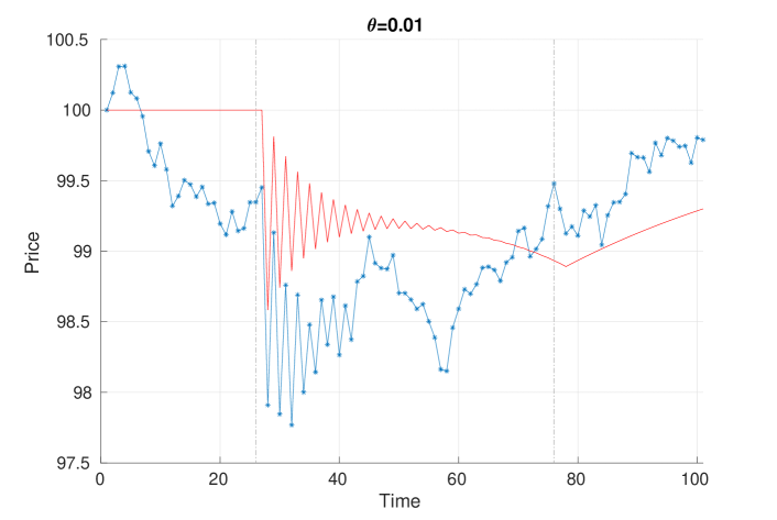
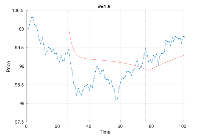
Figure 1: Blue lines exhibit the price process when both agents have inventory equals to $1$. The top (bottom) panel shows the dynamics when $\theta=0.01$ ($\theta=1.5$). The trading time grid has $N+1=51$ points, $G(t)=\exp(-t)$, the volatility of the unaffected price process is fixed to $1$ and $S_{0}=100$. The vertical grey dotted lines delineates the trading session. The red lines shows the drift dynamics due to trading.

Thus, citeschied2018market showed, when the trading time grid is equispaced, $\mathbb{T}_{N}$, and under general assumptions on $G$, the existence of a critical value $\theta^{*}=G(0)/4$ such that for $\theta<\theta^{*}$ the equilibrium strategies exhibit oscillations of buy and sell orders for both traders. Hence, the behavior at zero of the kernel function plays a relevant role for the equilibrium stability. Now, we recall the extension of this framework in a multi-agent market ($J>2$) of citeluo_schied. Then, we first extend their framework in the multi-asset ($M>1$) case, where we show the existence and uniqueness of the related Nash equilibrium. Finally, we generalize the stability result of citeschied2018market in the multi-asset case and we show how to appropriately scale with $J$ and $M$ the kernel function in order to prevent huge oscillations in the related equilibria.

2.1 The Luo and Schied multi-agent market impact model

The citeluo_schied model is an extension of the citeschied2018market model where $J$ risk-averse traders want to trade the same asset. The unaffected price process $S_{t}^{0}$ is always assumed to be a right continuous martingale in a suitable filtered probability space $(\Omega,\mathscr{F},(\mathscr{F}_{t})_{t\geq 0},\mathbb{P})$ and it is also required that $S_{\cdot}^{0}$ is a square-integrable process. As before, let $\mathbb{T}=\{t_{0},t_{1},\ldots,t_{N}\}$ be the trading time grid. Consistently with the previous notation, we denote with $\Xi=(\xi_{j,k})\in\mathbb{R}^{J\times(N+1)}$ the matrix of all strategies, where $\xi_{j,k}$ is the order flow of agent $j$ at time $t_{k}$, so that the affected price process is defined as

$$S_{t}^{\Xi}:=S_{t}^{0}-\sum_{t_{k}<t}G(t-t_{k})\cdot\sum_{j=1}^{J}\xi_{j,k},$$

where $G$ is the decay kernel. When comparing markets with a variable number of agents, differently from citeluo_schied, we will assume that the function $G$ can depend on $J$ (citeBagnoli, coimpact, see below). The generalization of admissible strategy is straightforward, indeed if $X_{j}$ denotes the inventory of the $j$-th agent, $\Xi$ is admissible for $\bm{X}\in\mathbb{R}^{J}$ and $\mathbb{T}$, if $\bm{\xi}_{j,\cdot}$ is admissible for $X_{j}$ and $\mathbb{T}$ for each $j$ according to definition 2.1, i.e., it is adapted to the filtration, bounded and $\sum_{k=0}^{N}\xi_{j,k}=X_{j}$. The set of admissible strategy is denoted as $\mathscr{X}(\bm{X},\mathbb{T})$. Then, if we consider all the possible time priorities among the $J$ traders at each time step, i.e. all the possible permutations that determine the time priority for each trading time $t_{k}$ assumed to be equiprobable, it is possible to generalize the previous definition of liquidation cost for a trader strategy, see citeluo_schied for further details. We denote $\Xi_{-j,\cdot}$ the matrix $\Xi$ where the $j$-th row is eliminated.

Definition 2.3 (citeluo_schied).

Given a time grid $\mathbb{T}$, the execution costs of a strategy $\bm{\xi}_{j,\cdot}$ given all other strategies $\bm{\xi}_{l,\cdot}$ where $l\neq j$ is defined as

$$C_{\mathbb{T}}(\bm{\xi}_{j,\cdot}|\Xi_{-j,\cdot})=\sum_{k=0}^{N}\bigg{(}\frac{G(0)}{2}\xi_{j,k}^{2}-S_{t_{k}}^{\Xi}\xi_{j,k}+\frac{G(0)}{2}\sum_{l\neq j}\xi_{j,k}\xi_{l,k}+\theta\ \xi_{j,k}^{2}\bigg{)},$$

where $\theta\geq 0$.

In the framework of citeschied2018market we have two risk-neutral agents which want to minimize the expected costs of a strategy, i.e. implementation shortfall orders. Now, following citeluo_schied, we consider the agents’ risk aversion by introducing the mean-variance and expected utility functionals, respectively

$$MV_{\gamma}(\bm{\xi}_{j,\cdot}|\Xi_{-j,\cdot}) :=\mathbb{E}[C_{\mathbb{T}}(\bm{\xi}_{j,\cdot}|\Xi_{-j,\cdot})]+\frac{\gamma}{2}\mbox{Var}[C_{\mathbb{T}}(\bm{\xi}_{j,\cdot}|\Xi_{-j,\cdot})],$$ (3)

$$U_{\gamma}(\bm{\xi}_{j,\cdot}|\Xi_{-j,\cdot}) :=\mathbb{E}[u_{\gamma}(-C_{\mathbb{T}}(\bm{\xi}_{j,\cdot}|\Xi_{-j,\cdot}))],$$ (4)

where $\gamma$ is the risk-aversion parameter and $u_{\gamma}(x)$ is the CARA utility function,

$$u_{\gamma}(x)=\begin{cases}\frac{1}{\gamma}(1-e^{-\gamma x})&\quad\text{if }\gamma>0,\\ x&\quad\text{if }\gamma=0.\end{cases}$$

As usual, see e.g. citealmgren2001optimal, the minimization of the mean-variance functional is restricted to deterministic admissible strategies, which is denoted as $\mathscr{X}_{\det}(\bm{X},\mathbb{T})$. All agents are assumed to have the same risk-aversion $\gamma\geq 0$, see citeluo_schied for further details. Moreover, they introduced the corresponding Nash equilibrium for the previously defined functionals.

Definition 2.4 (from citeluo_schied).

Given the time grid $\mathbb{T}$ and initial inventories $\bm{X}\in\mathbb{R}^{J}$ for $J$ traders with risk aversion parameter $\gamma\neq 0$, then:

• a Nash Equilibrium for mean-variance optimization is a matrix of strategies $\Xi^{*}\in\mathscr{X}_{\det}(\bm{X},\mathbb{T})$ such that each row $\bm{\xi}^{*}_{j,\cdot}$ minimizes the mean-variance functional
  $MV_{\gamma}(\bm{\xi}_{j,\cdot}|\Xi^{*}_{-j,\cdot})$ over $\bm{\xi}_{j,\cdot}\in\mathscr{X}_{\det}(X_{j},\mathbb{T})$;

• a Nash Equilibrium for CARA expected utility maximization is a matrix of strategies $\Xi^{*}\in\mathscr{X}(\bm{X},\mathbb{T})$ such that each row $\bm{\xi}_{j,\cdot}^{*}$ maximizes the CARA expected utility functional $U_{\gamma}(\bm{\xi}_{j,\cdot}|\Xi^{*}_{-j,\cdot})$ over $\bm{\xi}_{j,\cdot}\in\mathscr{X}(X_{j},\mathbb{T})$.

In particular, citeluo_schied showed that when the decay kernel is strictly positive definite and for any $\mathbb{T}$, parameters $\theta,\gamma\geq 0$ and initial inventories $\bm{X}\in\mathbb{R}^{J}$, there exists a unique Nash equilibrium for the mean-variance optimization which is given by

$$\bm{\xi}_{j,\cdot}^{*}=\overline{X}\bm{v}+(X_{j}-\overline{X})\bm{w},\quad j=1,2,\ldots,J,$$ (5)

where $\overline{X}=\frac{1}{J}\sum_{j=1}^{J}X_{j}$ and $\bm{v}$, $\bm{w}$ are the fundamental solutions defined as

$$\bm{v} =\frac{1}{\bm{e}^{T}[\Gamma^{\gamma,\theta}+(J-1)\widetilde{\Gamma}]^{-1}\bm{e}}[\Gamma^{\gamma,\theta}+(J-1)\widetilde{\Gamma}]^{-1}\bm{e}$$

$$\bm{w} =\frac{1}{\bm{e}^{T}[\Gamma^{\gamma,\theta}-\widetilde{\Gamma}]^{-1}\bm{e}}[\Gamma^{\gamma,\theta}-\widetilde{\Gamma}]^{-1}\bm{e},$$

and, if $\varphi(t):=\mbox{Var}(S_{t}^{0})$, for $t\geq 0$, the matrix $\Gamma^{\gamma,\theta}$ is defined for $\theta,\gamma\geq 0$ as

$$\Gamma_{i,j}^{\gamma,\theta}:=(\Gamma_{\theta})_{i,j}+\gamma\varphi(t_{i-1}\wedge t_{j-1}),\quad i,j=1,2,\ldots,N+1,$$

where $\Gamma_{\theta}$ is the previously defined kernel matrix. Moreover, if $S_{t}^{0}=S_{0}+\sigma B_{t}$, for $t\geq 0$, where $S_{0},\sigma>0$ are constants and $B_{t}$ is a standard Brownian motion, i.e., the unaffected price process is a Bachelier model, then (5) is also a Nash equilibrium for CARA expected utility maximization and it is unique if we restrict all trader strategies to be deterministic, see citeluo_schied for further details.

3 Multi-asset market impact games

We now extend the previous framework allowing the $J$ agents to trade a portfolio of $M>1$ assets. Indeed, agents often liquidate portfolio positions, which accounts in trading simultaneously many assets. In general, the optimal execution of a portfolio is different from many individual asset optimal executions, because of (i) correlation in asset prices, (ii) commonality in liquidity across assets (citeChordia), and (iii) cross-impact effects. In the following we will focus mainly on the third effect, even if disentangling them is a challenging statistical problem and we will discuss its relations with the correlation in asset prices which ensure the existence of Nash equilibrium.

To proceed, we first extend the notion of admissible strategy to the multi-asset case. A strategy for $J$ traders during the trading time interval $\mathbb{T}$ for $M$ assets is a multidimensional array $\Xi=(\xi_{i,j,k})\in\mathbb{R}^{M\times J\times(N+1)}$, where ${\xi}_{i,j,k}$ is the strategy for the $j$-th trader in the $i$-th asset at time step $k$. Straightforwardly, given a fixed time grid $\mathbb{T}$ and initial inventory $X\in\mathbb{R}^{M\times J}$, where each column $j$ contains the inventories of trader $j$ for the $M$ assets, a strategy $\Xi$ of random variables is admissible for $X$ if i) for all time step $k$, $\Xi_{\cdot,\cdot,k}$ is $\mathscr{F}_{t_{k}}$-measurable and bounded and ii) $\sum_{k=0}^{N}\bm{\xi}_{\cdot,j,k}=\bm{X}_{j}\in\mathbb{R}^{M}$ for each $j$, where $\bm{X}_{j}$ is the $j$-th column of $X$.

The second important point is that the trading of one asset modifies also the price of the other asset(s). This effect is termed cross-impact. While self-impact may be attributed to a mechanical and induced consequence of the order book, the cross-impact may be understood as an effect related to mispricing in correlated assets which are exploited by arbitrageurs betting on a reversion to normality, see citealmgren2001optimal and citeschneider2018cross for further details. Cross-impact has been empirically studied recently, see e.g. citemastromatteo2017trading, schneider2018cross and its role in optimal execution has been highlighted in citeGerry.

Mathematically cross-impact is modeled by introducing a function $\mathcal{Q}^{(J,M)}:\mathbb{R}_{+}\times\mathbb{R}^{M}\to\mathbb{R}^{M}$ describing how the trading of the $M$ assets affect their prices at a certain future time. Note that in general the cross-impact function might depend on the number of assets $M$ and on the number of agents $J$. Later we will discuss more in detail how this dependence affects market stability. citeschneider2018cross have discussed necessary conditions for the absence of price manipulation for multi-asset transient impact models. They have shown that the cross-impact function need to be symmetric and linear in order to avoid arbitrage and manipulations. Moreover, following example 3.1 of citealfonsi2016multivariate and as empirically observed by citemastromatteo2017trading, we assume the same temporal dependence of $G$ among the assets. Then, we assume that $\mathcal{Q}^{(J,M)}=Q\cdot G(t)$ where $Q$ is linear and symmetric, i.e., $Q\in\mathbb{R}^{M\times M}$ and $Q=Q^{T}$ and $G:\mathbb{R}_{+}\to\mathbb{R}_{+}$. Clearly the dependence from $J$ and $M$ can be in $Q$ and/or in $G(t)$. We also assume that $Q$ is a nonsingular matrix. Therefore, the price process during order execution is defined as

$$\bm{S}_{t}^{\Xi}=\bm{S}_{t}^{0}-\sum_{t_{k}<t}G(t-t_{k})\cdot Q\cdot\sum_{j=1}^{J}\bm{\xi}_{\cdot,j,k}$$

where we refer to $Q\in\mathbb{R}^{M\times M}$ as the cross-impact matrix, $\bm{S}_{t}^{0}\in\mathbb{R}^{M}$ is the unaffected price process which is assumed to be a right-continuous martingale defined on a suitable filtered probability space and it is a square-integrable process.

If for each asset the time priority among the traders is determined by considering all the possible permutations of agents for each trading time $t_{k}$, then, following the same motivation of citeschied2018market and citeluo_schied, the definition 2.3 of liquidation cost is generalized as follows:

Definition 3.1 (Execution Cost).

Given a time grid $\mathbb{T}$ and $\theta\geq 0$, the execution cost of a strategy $\Xi_{\cdot,j,\cdot}$ given all other strategies $\Xi_{\cdot,l,\cdot}$ where $l\neq j$ is defined as

$$\begin{split}C_{\mathbb{T}}(\Xi_{\cdot,j,\cdot}|\Xi_{\cdot,-j,\cdot})&=\sum_{k=0}^{N}\bigg{(}\frac{G(0)}{2}\langle Q\bm{\xi}_{\cdot,j,k},\bm{\xi}_{\cdot,j,k}\rangle-\langle\bm{S}_{t_{k}}^{\Xi},\bm{\xi}_{\cdot,j,k}\rangle+\\ &+\frac{G(0)}{2}\sum_{l\neq j}\langle Q\bm{\xi}_{\cdot,l,k},\bm{\xi}_{\cdot,j,k}\rangle+\theta\ \langle\bm{\xi}_{\cdot,j,k},\bm{\xi}_{\cdot,j,k}\rangle.\bigg{)}.\end{split}$$

The previous definition is motivated by the following argument. When only agent $j$ trades, the prices are moved from $\bm{S}_{t_{k}}^{\Xi}$ to $\bm{S}_{t_{k}+}^{\Xi}=\bm{S}_{t_{k}}^{\Xi}-G(0)Q\bm{\xi}_{\cdot,j,k}$. However, the order is executed at the average price and the player incurs in the expenses

$$-\frac{1}{2}\langle(\bm{S}_{t_{k}}^{\Xi}+\bm{S}_{t_{k}+}^{\Xi}),\bm{\xi}_{\cdot,j,k}\rangle=\frac{G(0)}{2}\langle Q\bm{\xi}_{\cdot,j,k},\bm{\xi}_{\cdot,j,k}\rangle-\langle\bm{S}_{t_{k}}^{\Xi},\bm{\xi}_{\cdot,j,k}\rangle.$$

Then, suppose that immediately after $j$ the agent $l$ place an order and the prices are moved linearly from $\bm{S}_{t_{k}+}^{\Xi}$ to $\bm{S}_{t_{k}+}^{\Xi}-G(0)Q\bm{\xi}_{\cdot,l,k}$, so the cost for $l$ is given by:

$$-\frac{1}{2}\langle(\bm{S}_{t_{k}+}^{\Xi}+\bm{S}_{t_{k}+}^{\Xi})-G(0)Q\bm{\xi}_{\cdot,l,k},\bm{\xi}_{\cdot,l,k}\rangle=\frac{G(0)}{2}\langle Q\bm{\xi}_{\cdot,l,k},\bm{\xi}_{\cdot,l,k}\rangle-\langle\bm{S}_{t_{k}}^{\Xi},\bm{\xi}_{\cdot,l,k}\rangle+G(0)\langle Q\bm{\xi}_{\cdot,j,k},\bm{\xi}_{\cdot,l,k}\rangle.$$

The term $G(0)\langle Q\bm{\xi}_{\cdot,j,k},\bm{\xi}_{\cdot,l,k}\rangle$ is the additional cost due to the latency, where on average for each asset half of the times the order of agent $j$ will be executed before the one of agent $l$, so that the latency costs for agent $j$ at time step $k$ is given by $\frac{G(0)}{2}\sum_{l\neq j}\langle Q\bm{\xi}_{\cdot,l,k},\bm{\xi}_{\cdot,j,k}\rangle$, see citeluo_schied for further details.

The mean-variance and CARA expected utility functionals are straightforwardly generalized using the previous defined execution cost. Indeed,

$$MV_{\gamma}(\Xi_{\cdot,j,\cdot}|\Xi_{\cdot,-j,\cdot}) :=\mathbb{E}[C_{\mathbb{T}}(\Xi_{\cdot,j,\cdot}|\Xi_{\cdot,-j,\cdot})]+\frac{\gamma}{2}\mbox{Var}[C_{\mathbb{T}}(\Xi_{\cdot,j,\cdot}|\Xi_{\cdot,-j,\cdot})],$$ (6)

$$U_{\gamma}(\Xi_{\cdot,j,\cdot}|\Xi_{\cdot,-j,\cdot}) :=\mathbb{E}[u_{\gamma}(-C_{\mathbb{T}}(\Xi_{\cdot,j,\cdot}|\Xi_{\cdot,-j,\cdot}))].$$ (7)

Therefore, we may define the related Nash equilibria definitions:

Definition 3.2.

Given the time grid $\mathbb{T}$ and initial inventories $X\in\mathbb{R}^{M\times J}$ for $M$ assets and $J$ traders with risk aversion parameter $\gamma\geq 0$, then:

• a Nash Equilibrium for mean-variance optimization is a multidimensional array of strategies $\Xi^{*}\in\mathscr{X}_{\det}(X,\mathbb{T})$ such that $\Xi_{\cdot,j,\cdot}^{*}$ minimizes the mean-variance functional $MV_{\gamma}(\Xi_{\cdot,j,\cdot}|\Xi^{*}_{\cdot,-j,\cdot})$ over $\Xi_{\cdot,j,\cdot}\in\mathscr{X}_{\det}(\bm{X}_{j},\mathbb{T})$;

• a Nash Equilibrium for CARA expected utility maximization is a multidimensional array of strategies $\Xi^{*}\in\mathscr{X}(X,\mathbb{T})$ such that each $\Xi_{\cdot,j,\cdot}^{*}$ maximizes the CARA expected utility functional $U_{\gamma}(\Xi_{\cdot,j,\cdot}|\Xi^{*}_{\cdot,-j,\cdot})$ over $\Xi_{\cdot,j,\cdot}\in\mathscr{X}(\bm{X}_{j},\mathbb{T})$.

We recall that $\bm{S}_{t}^{0}$ follows a Bachelier model if $\bm{S}_{t}^{0}=\bm{S}_{0}+L\bm{B}_{t}$ where $\bm{S}_{0}$ is a fixed vector and $\bm{B}_{t}$ is a multivariate (standard) Brownian motion, where its components are independent with unit variance so that the variance-covariance matrix of $\bm{S}_{t}^{0}$ is given by $\Sigma=LL^{T}$.

3.1 Nash equilibrium for the linear cross impact model

We now prove the existence and uniqueness of the Nash equilibrium in this multi-asset setting. This is achieved by using the spectral decomposition of $Q$ to orthogonalize the assets, which we call “virtual” assets, so that the impact of the orthogonalized strategies on the virtual assets is fully characterized by the self-impact, i.e., the transformed cross impact matrix is diagonal. Thus, the existence and uniqueness of the Nash equilibrium derives immediately by following the same argument as in citeschied2018market and citeluo_schied. All the proofs are given in Appendix LABEL:app_1.

Remark 3.3.

If we suppose that $Q$ is the identity matrix, then the multi-asset market impact game is a straightforward generalization of the citeluo_schied model. Indeed, each order of the players for the $i$-th stock does not affect any other asset.

In general, if we assume that $\bm{S}_{t}^{0}$ has uncorrelated components, i.e., the variance-covariance matrix $\Sigma$ is diagonal, then the following result holds.

Lemma 3.4 (Nash Equilibrium for Diagonal Cross-Impact Matrix).

If $\bm{S}_{t}^{0}$ has uncorrelated components, for any strictly positive definite decay kernel $G$, time grid $\mathbb{T}$, parameters $\theta,\gamma\geq 0$, initial inventory $X\in\mathbb{R}^{M\times J}$ and diagonal positive cross impact matrix $D=\mbox{diag}(\lambda_{1},\lambda_{2},\ldots,\lambda_{M})$, there exists a unique Nash Equilibrium $\Xi^{*}\in\mathscr{X}_{\det}(X,\mathbb{T})$ for the mean-variance optimization problem and it is given by

$$\bm{\xi}_{i,j,\cdot}^{*}=\overline{X}_{i,\cdot}\bm{v}_{i}+(X_{i,j}-\overline{X}_{i,\cdot})\bm{w}_{i},\quad j=1,2,\ldots,J,\quad i=1,2,\ldots,M,$$ (8)

where $\overline{X}_{i,\cdot}=\frac{1}{J}\sum_{j=1}^{J}X_{i,j}$, $\bm{v}_{i}$ and $\bm{w}_{i}$ are the fundamental solutions associated with the decay kernel $G_{i}(t)=G(t)\cdot\lambda_{i}$ and same parameter $\theta$. Moreover, if $\bm{S}^{0}_{t}$ follows a Bachelier model, then (8) is also a Nash equilibrium for CARA expected utility maximization.

Remark 3.5.

We observe that for risk-neutral agents, i.e., $\gamma=0$, the assumptions of uncorrelated assets is no more necessary to prove Lemma 3.4. Indeed, the mean-variance functional is restricted only to the expected cost and for linearity $MV_{0}(\Xi_{\cdot,j,\cdot}|\Xi_{\cdot,-j,\cdot})=\sum_{i=1}^{M}MV_{0}(\bm{\xi}_{i,j,\cdot}|\Xi_{i,-j,\cdot};G_{i})$, where $MV_{0}(\bm{\xi}_{i,j,\cdot}|\Xi_{i,-j,\cdot};G_{i})=\mathbb{E}[C_{\mathbb{T}}(\bm{\xi}_{i,j,\cdot}|\Xi_{i,-j,\cdot};G_{i})]$ is the expected cost of Definition 2.3 where the decay kernel is multiplied by $\lambda_{i}$, and we have the same conclusion of Lemma 3.4 regardless the covariance matrix of $\bm{S}_{t}^{0}$.

We first introduce some notation and then we state the main results. We say that assets are orthogonal if the corresponding cross-impact matrix is diagonal. Let us consider the spectral decomposition of $Q$, i.e., $QV=VD$, where $V$ and $D$ are the orthogonal and diagonal matrices containing the eigenvectors and eigenvalues, respectively. Since we assume that $Q$ is a non singular symmetric matrix, then $D$ is diagonal with all elements different from zero. We define the prices of the virtual assets as $\bm{P}_{t}:=V^{T}\bm{S}_{t}^{\Xi}$ and we observe that

$$\begin{split}\bm{P}_{t}&=\bm{P}_{t}^{0}-\sum_{t_{k}<t}G(t-t_{k})\cdot D\cdot V^{T}\cdot\bigg{(}\sum_{j=1}^{J}\bm{\xi}_{\cdot,j,k}\bigg{)}\\ &=\bm{P}_{t}^{0}-\sum_{t_{k}<t}G(t-t_{k})\cdot D\cdot\bigg{(}\sum_{j=1}^{J}\bm{\xi}^{P}_{\cdot,j,k}\bigg{)},\end{split}$$ (9)

where $\bm{P}_{t}^{0}:=V^{T}\bm{S}_{t}^{0}$ and $\bm{\xi}_{\cdot,j,k}^{P}:=V^{T}\bm{\xi}_{\cdot,j,k}$. This last quantity is the strategy of trader $j$ at time step $k$ in the virtual assets, which is admissible for inventory $\bm{X}_{j}^{P}=V^{T}\bm{X}_{j}$, i.e, $\sum_{k=0}^{N}\bm{\xi}_{\cdot,j,k}^{P}=\sum_{k=0}^{N}V^{T}\bm{\xi}_{\cdot,j,k}=V^{T}\bm{X}_{j}$. The virtual assets are mutually orthogonal by construction and their corresponding (virtual) decay kernels $G_{i}(t)$ are obtained as the product of the original decay kernel $G(t)$ and the corresponding eigenvalues $\lambda_{i}$ of the cross impact matrix, i.e., the decay kernel associated with the $i$-th virtual asset is $G_{i}(t):=G(t)\cdot\lambda_{i}$. Indeed, from Equation (9) the decay kernel $G(t)$ is multiplied by the eigenvalues of the cross impact matrix for each trading time $t_{k}$,

$$G(t-t_{k})\cdot D=\begin{bmatrix}G(t-t_{k})\lambda_{1}\\ &G(t-t_{k})\lambda_{2}\\ &&\ddots\\ &&&G(t-t_{k})\lambda_{M}\end{bmatrix}.$$

Then, as observed in Remark 3.3, the multi-asset market impact game where each asset is orthogonal to others is equivalent to $M$ one-asset market impact games, i.e., citeluo_schied models. The (virtual) decay kernels $G_{i}(t)$ satisfy the assumptions of strictly positive definite kernels as far as $\lambda_{i}>0\ \forall i=1,2,\ldots,M$, i.e., $Q$ is positive definite (see also citealfonsi2016multivariate). If $\mbox{Cov}(\bm{S}_{t}^{0})=\Sigma$, then $\mbox{Cov}(\bm{P}_{t}^{0})=V^{T}\Sigma V$. So, if $Q$ and $\Sigma$ are simultaneously diagonalizable then $\mbox{Cov}(\bm{P}_{t}^{0})$ is diagonal, i.e., the components of $\bm{P}_{\cdot}^{0}$ are uncorrelated and by Lemma 3.4 we obtain the associated Nash equilibria $\Xi^{*,P}$, whose components are defined as

$$\bm{\xi}_{i,j,\cdot}^{*,P}=\overline{X}_{i,\cdot}^{P}\bm{v}_{i}+(X_{i,j}^{P}-\overline{X}_{i,\cdot}^{P})\bm{w}_{i},\quad j=1,2,\ldots,J,\quad i=1,2,\ldots,M,$$ (10)

where $\overline{X}_{i,\cdot}^{P}=\frac{1}{J}\sum_{j=1}^{J}X^{P}_{i,j}$ is the average inventory on the $i$-th virtual asset among the traders and $\bm{v}_{i}$ and $\bm{w}_{i}$ are the previously defined fundamental solutions of citeluo_schied for the $i$-th virtual asset $P_{\cdot,i}$. For them, the decay kernel is given by $G_{i}(t)=G(t)\cdot\lambda_{i}$ and the corresponding $\varphi_{i}(t)$ is given by $\mbox{Var}(P_{t,i}^{0})$. Since, $Q$ and $\Sigma$ are both symmetric, so diagonalizable, $Q$ and $\Sigma$ are simultaneously diagonalizable if and only if $Q$ and $\Sigma$ commute. Therefore, we consider the following assumption.

Assumption 1.

The cross-impact matrix, $Q$, and the covariance matrix of the unaffected price process $\bm{S}_{t}^{0}$, $\Sigma$, commute, i.e., $Q\Sigma=\Sigma Q.$

This assumption is frequently made in the literature and approximately valid in real data, e.g., citemastromatteo2017trading makes this assumption on the correlation matrix. The empirical observation that the matrix $Q$ has a large eigenvalue with a corresponding eigenvector with almost constant components (as the market factor) and a block structure with blocks corresponding to economic sectors (as in the correlation matrix) indicates that the eigenvectors of $Q$ and $\Sigma$ are the same, i.e. that $Q$ and $\Sigma$ (approximately) commute. Notice also that citegarleanu2013dynamic propose a model of optimal portfolio execution where the quadratic transaction cost is characterized by a matrix which is proportional to $\Sigma$.

We enunciate the following theorem of existence and uniqueness of Nash equilibrium which extends Theorem 2.4 of citeluo_schied.

Theorem 3.6 (Nash Equilibrium for Multi-Asset and Multi-Agent Market Impact Games).

For any strictly positive definite decay kernel $G$, time grid $\mathbb{T}$, parameter $\theta,\gamma\geq 0$, initial inventory $X\in\mathbb{R}^{M\times J}$ and symmetric positive definite cross impact matrix $Q$ such that Assumption 1 holds, there exists a unique Nash Equilibrium $\Xi^{*}\in\mathscr{X}_{\det}(X,\mathbb{T})$ for the mean-variance optimization problem and it is given by

$$\Xi_{\cdot,j,\cdot}^{*}=V\Xi_{\cdot,j,\cdot}^{*,P},\quad j=1,2,\ldots,J$$ (11)

where $V$ is the matrix of eigenvectors of $Q$ and $\Xi^{*,P}\in\mathscr{X}_{\det}(X^{P},\mathbb{T})$ is the Nash Equilibrium (10) of the corresponding orthogonalized virtual asset market impact game where $X^{P}=V^{T}X$. Moreover, if $\bm{S}^{0}$ follows a Bachelier model then (11) is also a Nash equilibrium for CARA expected utility maximization.

However, we observe that for risk-neutral agents, i.e., $\gamma=0$, Assumption 1 is unnecessary. We remark this result in the following Corollary.

Corollary 3.7.

If the agents are risk-neutral, i.e., $\gamma=0$, then for any strictly positive definite decay kernel $G$, time grid $\mathbb{T}$, parameter $\theta\geq 0$, initial inventories $X\in\mathbb{R}^{M\times J}$ and symmetric positive definite cross impact matrix $Q$, there exists a unique Nash Equilibrium $\Xi^{*}\in\mathscr{X}_{\det}(X,\mathbb{T})$ for the mean-variance optimization problem and it is given by

$$\Xi_{\cdot,j,\cdot}^{*}=V\Xi_{\cdot,j,\cdot}^{*,P},\quad j=1,2,\ldots,J$$ (12)

where $V$ is the matrix of eigenvectors of $Q$ and $\Xi^{*,P}\in\mathscr{X}_{\det}(X^{P},\mathbb{T})$ is the Nash Equilibrium associated to the corresponding orthogonalized virtual asset market impact game where $X^{P}=V^{T}X$ . Moreover, if $\bm{S}^{0}_{t}$ follows a Bachelier model then (12) is also a Nash equilibrium over the set $\mathscr{X}(X,\mathbb{T})$.

4 Trading Strategies in Market Impact Games

Before studying market stability we investigate how the cross-impact effect and the presence of many competitors may affect trading strategies, in terms of Nash equilibria. To understand the rich phenomenology that can be observed in a market impact game, we introduce three types of traders:

• the Fundamentalist wants to trade one or more assets in the same direction (buy or sell). Notice that a Fundamentalist can have zero initial inventory for some assets;

• the Arbitrageur has a zero inventory to trade in each asset and tries to profit from the market impact payed by the other agents;

• the Market Neutral has a non zero volume to trade in each asset, but in order to avoid to be exposed to market index fluctuations, the sum of the volume traded in all assets is zero.

We remark that an Arbitrageur is a particular case of a Market Neutral agent in the limit case when the volume to trade in each asset is zero. Clearly in a single-asset market we have only two types of the previous agents, since a Market Neutral strategy requires at least two assets.

4.1 Cross-impact effects and liquidity strategies

To better understand how cross-impact affects optimal liquidation strategies, we consider the case of two risk-neutral agents which can (but not necessarily must) trade $M$ assets. We show below that the presence of multiple assets and of cross-impact can affect the trading strategy of an agent interested in liquidating only one asset. In particular, we find, counterintuitively, that it might be convenient for such an agent to trade (with zero inventory) the other asset(s) in order to reduce transaction costs.

We focus on the two-asset case, $M=2$, and we analyse the Nash equilibrium when the kernel function has an exponential decay, $G(t)=e^{-t}$. The first trader is a Fundamentalist who wants to liquidate the position in the first asset, i.e., $X_{1,1}=1$, while the second agent is an Arbitrageur, i.e., $X_{1,2}=0$. We set an equidistant trading time grid with $26$ points and $\theta=1.5$. The second asset is available for trading, but let us consider as a benchmark case when both agents trade only the first asset. This is a standard citeschied2018market game. Figure 2 exhibits the Nash Equilibrium for the two players. We observe that the optimal solution for the Fundamentalist is very close to the classical U-shape derived under the Transient Impact Model (TIM), i.e., our model when only one agent is present. However, the solution is asymmetric and it is more convenient for the Fundamentalist to trade more in the last period of trading. This can be motivated by observing that at equilibrium the Arbitrageur places buy order at the end of the trading day, and thus she pushes up the price. Then, the Fundamentalist exploits this impact to liquidate more orders at the end of the trading session. We remark that the Arbitrageur earns at equilibrium, since her expected cost is negative (see the caption).

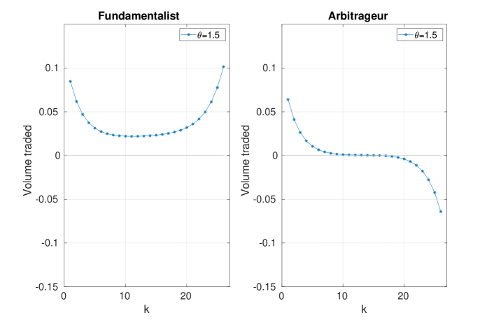
Figure 2: Nash equilibrium $\bm{\xi}_{1}^{*}$ of the Fundamentalist and $\bm{\xi}_{2}^{*}$ of the Arbitrageur trading only one asset. The trading time grid is equidistant with 26 points and $\theta=1.5$. The expected costs are equal to $\mathbb{E}[C_{\mathbb{T}}(\bm{\xi}_{1}^{*}|\bm{\xi}_{2}^{*})]=0.4882$, $\mathbb{E}[C_{\mathbb{T}}(\bm{\xi}_{2}^{*}|\bm{\xi}_{1}^{*})]=-0.0370$.

Now we examine the previous situation when the two traders solve the optimal execution problem taking into account the possibility of trading the other asset. We define the cross impact matrix $Q=\begin{bmatrix}1&q\\ q&1\end{bmatrix}$, where $q=0.6$. In Figure 3 we report the optimal solution where the inventory of the agents are set to be ${\bm{X}}_{1}=\begin{pmatrix}1&0\end{pmatrix}^{T}$ and ${\bm{X}}_{2}=\begin{pmatrix}0&0\end{pmatrix}^{T}$. The Fundamentalist wants to liquidate only one asset, but, as clear from the Nash equilibrium, the cross-impact influences the optimal strategies in such a way that it is optimal for him/her to trade also the other asset. In terms of cost, for the Fundamentalist trading the two assets is worse off than in the benchmark case (see the values of $\mathbb{E}[C_{\mathbb{T}}(\Xi_{\cdot,1,\cdot}^{*}|\Xi_{\cdot,2,\cdot}^{*})]$ in captions). However, if the Fundamentalist trades only asset 1 and Arbitrageur trades both assets, the former has a cost of $0.4935$ which is greater than the expected costs associated with Figure 3. Thus, the Fundamentalist must trade the second asset if the Arbitrageur does (or can do it).

For completeness in Table 1 we compare the expected costs of both Fundamentalist and Arbitrageur when the two agents may decide to trade i) both assets, i.e., they consider market impact game and cross-impact effect, or ii) one asset, i.e., they only consider the market impact game. It is clear that both agents prefer to trade both assets. Actually, the state where both agents trade two assets is the Nash equilibrium of the game where each agent can choose how many assets to trade.

		Arbitrageur
		$1$ Asset	$2$ Asset
Fundamentalist	$1$ Asset	$(0.4882,-0.0370)$	$(0.4935,-0.0412)$
	$2$ Asset	$(0.4836,-0.0334)$	${\bm{(}0.4885,-0.0377)}$

Table 1: Payoff matrix of expected costs when the Fundamentalist and Arbitrageur inventories are equal to $(1\leavevmode\nobreak\ 0)^{T}$ and $(0\leavevmode\nobreak\ 0)^{T}$, respectively. We have highlighted in red the Nash Equilibrium associated with this payoff matrix. The payoff in the $i$-th row and $j$-th column correspond to the game when the Fundamentalist and Arbitrageur decide to trade $i$ and $j$ assets, respectively, i.e., the element in the first row and second column is the payoff when the Fundamentalist trades only the first asset while the Arbitrageur trades both assets.

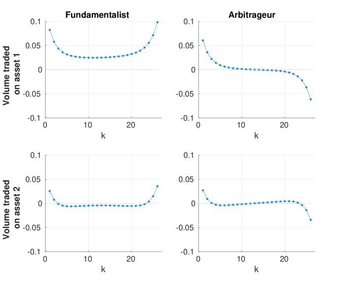
Figure 3: Optimal strategies for a Fundamentalist ($\Xi_{\cdot,1,\cdot}^{*}$) and an Arbitrageur ($\Xi_{\cdot,2,\cdot}^{*}$), where their inventories are equal to $(1\leavevmode\nobreak\ 0)^{T}$ and $(0\leavevmode\nobreak\ 0)^{T}$, respectively. $Q=\begin{bmatrix}1&0.6\\ 0.6&1\end{bmatrix}$, and the trading time grid is an equidistant time grid with $26$ points. The expected costs are equal $\mathbb{E}[C_{\mathbb{T}}(\Xi_{\cdot,1,\cdot}^{*}|\Xi_{\cdot,2,\cdot}^{*})]=0.4885$, $\mathbb{E}[C_{\mathbb{T}}(\Xi_{\cdot,2,\cdot}^{*}|\Xi_{\cdot,1,\cdot}^{*})]=-0.0377$ when $\theta=1.5$.

The solution presented above is generic, but an important role is played by the transaction cost modeled by the temporary impact. When the temporary impact parameter $\theta$ increases, the benefit of the cross-impact vanishes, and the optimal strategy of the Fundamentalist tends to the solution provided by the simple TIM with one asset and no other agent. We find that the difference between these expected costs is negative, i.e. it is always optimal to trade also the second asset, but converges to zero for large $\theta$, see Figure 4 panel (a). Furthermore, it is worth noting that, if $S=\sum_{k}|\xi_{k,2}|$ denotes the total absolute volume traded by the Fundamentalist on the second asset, then $\lim_{\theta\to 0}S=0$ and $\lim_{\theta\to\infty}S=0$ as exhibited from Figure 4 panel (b). This means, that when the cost of trades increases, it is not anymore convenient for both traders to try to exploit the cross impact effect.

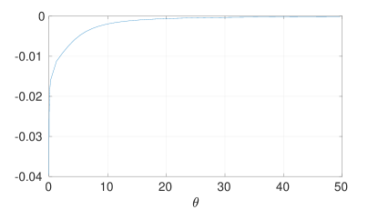
(a)

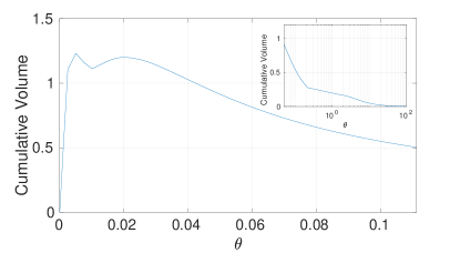
(b)

Figure 4: Figure (a). The y axis shows the difference between the expected cost of the Fundamentalist when he/she consider the cross-impact effect and the Arbitrageur and the expected cost when he/she places order following the classical one asset TIM model and the x axis the cost parameter $\theta$. Figure (b). Cumulative traded volume of the second asset by the Fundamentalist when playing against an Arbitrageur as a function of $\theta$. The inset shows the same curve in semi-log scale. The setting is the same of Figure 3.

4.2 Do arbitrageurs act as market makers at equilibrium?

We now consider the cases when the agents are of different type. In particular, we focus on the role of an Arbitrageur as an intermediary between two Fundamental traders of opposite sign. When a Fundamental seller and a Fundamental buyer trade the same asset(s), are the Arbitrageurs able to profit, acting as a sort of market maker by buying from the former and selling to the latter?

To answer this question, we compute the Nash equilibrium of a market impact game with $M=2$ assets and $J=3$ agents, namely a Fundamentalist seller with inventory $(1\ 0)^{T}$, a Fundamentalist buyer with inventory $(-1\ 0)^{T}$, and an Arbitrageur. We assume that agents are risk-neutrals, $\gamma=0$, and $Q=\begin{bmatrix}1&0.6\\ 0.6&1\end{bmatrix}$. As panels (a) of Figure 5 show, the Arbitrageur does not longer trade and the expected costs are $0.1056$ and $0$ for the two Fundamentalists and the Arbitrageur, respectively. This indicates that the two Fundamentalists are able to reduce significantly their costs with respect to the previous case, increasing their protection against predatory trading strategies and that the Arbitrageur is unable to act as a market maker. The previous cases are particular examples of the following more general result.

Proposition 4.1.

Under the assumptions of Theorem 3.6, the following are equivalent:

• The aggregate net order flow is zero for each asset, i.e.,

  $$\overline{X}_{i,\cdot}=\frac{1}{J}\sum_{j=1}^{J}X_{i,j}=0\quad\forall i=1,2,\ldots,M;$$

• The optimal solution for an Arbitrageur is equal to zero for all assets.

In other words, when the aggregate net order flow is zero for each asset then there are no arbitrageurs in the market, i.e., the Nash equilibrium for Arbitrageurs is zero, so that the optimal schedule corresponds to place no orders in the market.

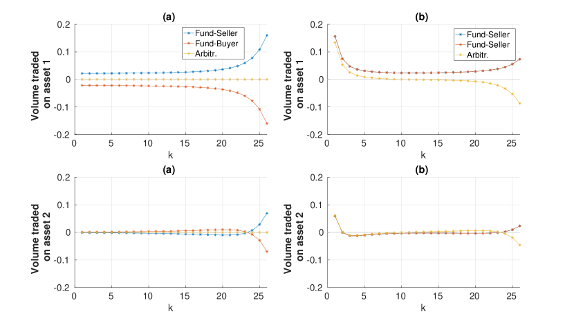
Figure 5: Optimal schedule for market impact game with $M=2$ assets and $J=3$ risk-neutral agents. Panels (a) exhibit the optimal schedule for a Fundamentalist seller, buyer (with inventory $(1\ 0)^{T}$ and $(-1\ 0)^{T}$, respectively), and an Arbitrageur. Panels (b) exhibit the optimal schedule for two identical Fundamentalist sellers (with inventories $(1\ 0)^{T}$, respectively), and an Arbitrageur. Blue and red lines are the Nash equilibrium for the Fundamentalist traders. The yellow line refers to the equilibrium of the Arbitrageur. The trading time is equidistant with $26$ points, where the cross impact is set to $q=0.6$, $\gamma=0$ and $\theta=1.5.$

As a comparison, we consider two identical Fundamentalist sellers (with inventories $(1\ 0)^{T}$) and the other parameters are the same as above. Figure 5, panels (b), displays the equilibrium solution. The solution of the Fundamentalists are identical. While the trading pattern of the Arbitrageur is qualitatively similar to the one of the two agent case (see Fig. 3), the Fundamentalists trade significantly less toward the end of the day. This is likely due to the fact that it might be costly to trade for one Fundamentalist given the presence of the other. The expected costs of the two Fundamentalists is equal to $0.8911$ (which is approximately two times of the two players game) and $-0.0996$ for the Arbitrageur.

5 Instabilities in Market Impact Games

We now turn to our attention to the study of market stability. Since the seminal work of citeschied2018market we known that, when two risk-neutral agents trade one asset, stability is fully determined by the value $\theta$ of the transaction cost, see Theorem 2.7 of citeschied2018market. Here we extend their results for the multi-asset case and we derive a general result which involves the spectrum of the cross-impact matrix. However, the proof of