Large-Momentum Effective Theory

Abstract

Since the parton model was introduced by Feynman more than fifty years ago, we have learned much about the partonic structure of the proton through a large body of high-energy experimental data and dedicated global fits. However, calculating the partonic observables such as parton distribution function (PDFs) from the fundamental theory of strong interactions, QCD, has made limited progress. Recently, the authors have advocated a formalism, large-momentum effective theory (LaMET), through which one can extract parton physics from the properties of the proton travelling at a moderate boost-factor, e.g., $\gamma\sim(2-5)$. The key observation behind this approach is that Lorentz symmetry allows the standard formalism of partons in terms of light-front operators to be replaced by an equivalent one with large-momentum states and time-independent operators of a universality class. With LaMET, the PDFs, generalized PDFs or GPDs, transverse-momentum-dependent PDFs, and light-front wave functions can all be extracted in principle from lattice simulations of QCD (or other non-perturbative methods) through standard effective field theory matching and running. Future lattice QCD calculations with exa-scale computational facilities can help to understand the experimental data related to the hadronic structure, including those from the upcoming Electron-Ion Colliders dedicated to exploring the partonic landscape of the proton. Here we review the progress made in the past few years in development of the LaMET formalism and its applications, particularly on the demonstration of its effectiveness from initial lattice QCD simulations.

I Introduction

The proton and neutron, collectively called the nucleon, are the basic building blocks of visible matter in the universe today. Ever since they were discovered in laboratories nearly a century ago Rutherford (1919); Chadwick (1932), their fundamental properties have been vigorously explored: from the determination of the spin through the specific heat of liquid hydrogen Dennison (1927), to the measurement of the magnetic moments Estermann et al. (1933), and the extraction of their electromagnetic sizes through elastic electron scattering  Hofstadter (1956). The most revealing discovery, however, came from the electron deep-inelastic scattering (DIS) on the proton and nuclei at Stanford Linear Accelerator Center (SLAC) in the late 1960s, in which the constituents of the proton and neutron, quarks (and later gluons), were discovered Bloom et al. (1969). Soon after, quantum chromodynamics (QCD), a quantum field theory (QFT) based on “color” SU(3) gauge symmetry, was established as the fundamental theory of strong interactions Fritzsch et al. (1973); Gross and Wilczek (1973); Politzer (1973), and of the internal structure of the nucleon as well Thomas and Weise (2001).

During the last fifty years, significant progress has been made in understanding the nucleon’s internal structure in both experiment and theory. Multiple experimental facilities have been built to study high-energy collisions involving protons and nuclei, from which a large amount of experimental data has been accumulated. Based on the QCD factorization theorems Collins (2011a), derived from perturbative QCD analyses beyond Feynman’s parton model Feynman (1972), the parton distribution functions (PDFs), which characterize the longitudinal momentum distributions of quarks and gluons in hadrons moving at infinite momentum, have been obtained from global fits to these data Gao et al. (2018); Hou et al. (2019); Harland-Lang et al. (2015); Ball et al. (2017). A recent result of the phenomenological proton PDFs is shown in Fig. 1 where $x$ is the momentum fraction of the proton carried by partons. The PDFs provide a comprehensive description of the quark and gluon content of the nucleon. On the theoretical frontier, the Euclidean path-integral formalism of QCD, combined with the lattice regularization and Monte Carlo simulations Wilson (1974), has offered a systematic way of performing ab initio calculations of non-perturbative strong interactions. The rapid rise in computational power and development of intelligent numerical algorithms have made such a lattice QCD approach extremely successful in computing hadron spectroscopy, the strong coupling, hadronic form factors, etc., and even scattering phase shifts Tanabashi et al. (2018); Briceno et al. (2018); Aoki et al. (2020).

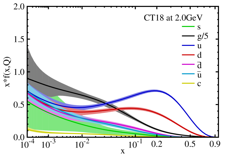
Figure 1: Phenomenological parton distributions obtained by the CTEQ-TEA collaboration (CT18) from fits to global high-energy scattering data Hou et al. (2019), where $0\leq x\leq 1$ is the fraction of the proton’s infinite momentum carried in a parton.

Despite these impressive achievements, we have not been able to systematically explain the partonic structure of the proton from first principles, or more explicitly, we have not made fundamental progress in computing the quark and gluon distributions starting from the QCD Lagrangian (see Sec. I.3 for a brief summary). There is actually a good reason behind it: The standard formulation of parton physics in the textbooks Sterman (1993); Collins (2011a) is accomplished through the dynamical correlators of quark and gluon fields on the light-front (LF) defined by $t-z={\rm const.}$, which has the important feature of being independent of the proton’s momentum. On the other hand, lattice QCD is formulated in the Euclidean space with imaginary time, and cannot be used to directly calculate the dynamical correlations that depend on real time. The standard lattice approach to parton physics has been to calculate the lower moments of parton distributions, which are matrix elements of local operators Lin et al. (2018c). However, the limitations to the first few moments prohibit practitioners from reproducing reliably the $x$-dependent structure as shown in Fig. 1, other than fitting model functional forms. Over the years, Hamiltonian diagonalization in LF quantization (LFQ) Brodsky et al. (1998) and Schwinger-Dyson equations Maris and Roberts (2003) have been proposed to solve the nucleon structure as Minkowskian approaches. Although significant advances have been made phenomenologically, a systematic approximation to calculate the nucleon PDFs is still missing.

A few years ago, some of the present authors proposed a general approach to calculate $x$-dependent parton distributions based on Feynman’s original idea about partons: They are the infinite-momentum limit of static properties of the proton at large momentum, and therefore are intrinsically Euclidean quantities accessible through lattice QCD Ji (2013); Ji et al. (2013b); Ji (2014). According to this, parton physics in an intermediate range of $x_{\rm min}\sim 0.1<x<x_{\rm max}\sim 0.9$ can be calculated from the physical properties of the proton at a moderately-large momentum, e.g., with a Lorentz boost factor $\gamma=2-5$. The theory has been named as large-momentum effective theory (LaMET) because a rigorous connection between the infinite-momentum frame (IMF) partons and quarks and gluons at a finite momentum requires proper account of the ultraviolet (UV) modes with large momentum in effective field theory (EFT) and systematic power counting.

The basic principle for LaMET comes from an implicit observation in the naive parton model: The structure of the proton is approximately independent of its momentum so long as it is much larger than a typical strong-interaction scale $\Lambda_{\rm QCD}$, or its mass. For example, the quark momentum distribution at moderate $x$ in the proton at $P=|\vec{P}|=5$ GeV is not very different from that at $P=50$ GeV or $P=5$ TeV. One might call this phenomenon large-momentum symmetry, the nature of which is similar to that of the electronic structure of the hydrogen atom is not sensitive to the proton mass, so long as it is much larger than that of the electron. The asymptotic behavior of the proton structure might be controlled by an expansion in $\Lambda_{\rm QCD}/P$, but a justification would require a better understanding of the underlying dynamics. Assuming this, Feynman replaced the protons probed at large but finite momenta in high-energy scattering with the one at infinite momentum $P=\infty$, corresponding to the leading term in the $\Lambda_{\rm QCD}/P$ expansion, and therefore the idealized concepts of the proton in the IMF and its constituents—partons—were born.

In QFTs, however, the existence of the $P=\infty$ limit depends on their UV behavior. In general, the infinite-momentum limit does not commute with the UV cut-off limit $\Lambda_{\rm UV}\to\infty$. While the physical limit is $(\Lambda_{\rm UV}\gg P)\to\infty$, the parton model and subsequent QCD factorization theorems use $(P\gg\Lambda_{\rm UV})\to\infty$, keeping all PDFs with the finite support $|x|\leq 1$ where negative $x$ is for antiquarks. Thus partons are an idealized concept which does not exist in the real world. Fortunately, because of asymptotic freedom, the above differences can be calculated in perturbative QCD. Therefore, LaMET is an effective theory of partons, which uses the ordinary field theoretical calculations $(\Lambda_{\rm UV}\gg P)\to\infty$ and systematically takes into account non-commuting $P\to\infty$ limits through EFT matching and running and finite $P$ effects by power corrections. Thus, the PDFs defined in the IMF or on the LF can be accessed at moderate $x$ from the structure calculations at $P\sim$ a few GeVs.

The first application of LaMET was to the total gluon helicity $\Delta G$ in the polarized proton, a quantity of significant experimental interest at the polarized RHIC Bunce et al. (2000), but not within theoretical reach for many years. In Ji et al. (2013b), we have shown that from a large-momentum matrix element of the gluon spin operator in a physical gauge, $\Delta G$ can be obtained through an EFT matching. Following this success, LaMET was applied to the collinear quark PDFs Ji (2013). This latter application has generated considerable theoretical as well as numerical activities, particularly for the flavor non-singlet $u-d$ distributions in the proton and other hadrons. A general LaMET framework was subsequently introduced in Ji (2014). More recently, the approach has been extended to the gluons as well Zhang et al. (2019b); Li et al. (2019). Therefore, the PDFs can now be computed directly in lattice QCD at specific Feynman variable $x$, without using LFQ. Besides, the partonic landscape of the proton is extremely rich, and LaMET holds the promise of computing parton physics beyond the collinear PDFs.

In recent years, tremendous progress has been made in formulating new parton observables for the proton. In particular, two parallel concepts have been developed in characterizing the transverse structure of the proton. The first is the generalized parton distributions (GPDs) Müller et al. (1994); Ji (1997b); Radyushkin (1999). The GPDs combine the features of the proton’s elastic form factors, which provide the transverse-space density of partons Miller (2007), and Feynman PDFs, and interpolate them. Given the joint longitudinal-momentum and transverse-space distributions, one can construct the orbital angular momentum (OAM) of partons, among others Ji (1997b). In general, the GPDs can be used to generate momentum-dissected transverse space images of the proton Burkardt (2000). A new class of experimental processes, deeply-virtual exclusive processes (DVEP), including deeply-virtual Compton scattering (DVCS) in which the final state is a diffractive real photon plus a recoiling proton, has been found to measure them Ji (1997b, a). The second concept is the transverse-momentum-dependent (TMD) PDFs (or TMDPDFs), in which the parton’s transverse momentum is explicit Collins and Soper (1981); Collins (2011a). Much theoretical progress has been made in recent years regarding their proper definitions, factorizations, and spin correlations Collins and Rogers (2013); Echevarría et al. (2013); Collins and Rogers (2017). TMDPDFs can be measured in experimental processes by observing the transverse momentum of the final-state particles.

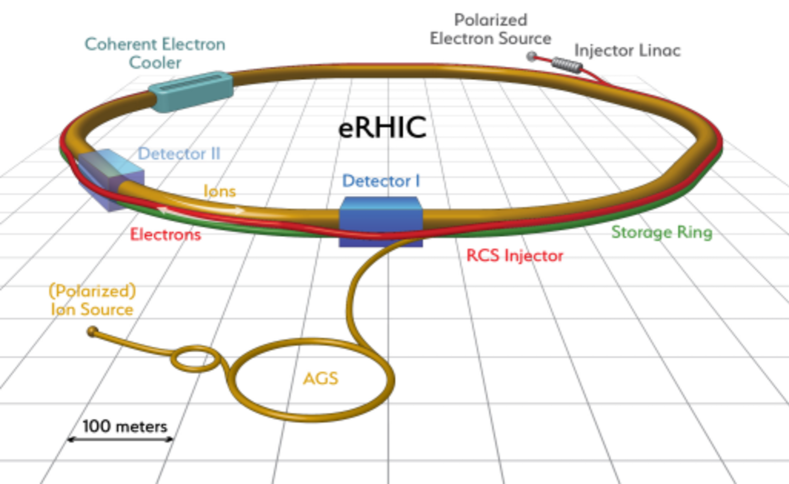
Figure 2: A realization of Electron-Ion Collider at BNL (figure credit to BNL), which can be used to probe the partonic landscape of the proton.

Over the years, it has gradually become clear that a dedicated experimental facility to fully explore the partonic landscape of the proton is required. To meet this requirement, the US nuclear science community has proposed, to build a high-energy, high-luminosity Electron-Ion Collider (EIC) Aprahamian et al. (2015), which has been recently approved by the US Department of Energy. The new collider accelerates electrons to 10-30 GeV and ions— including the proton and heavy nuclei all the way up to Pb or U— up to 100 GeV per nucleon, realizing the center-of-mass collision energy $E_{\rm cm}$ from 40 to 170 GeV. The corresponding electron energy in fixed-target experiments would be 100 GeV to 10 TeV. The beams are polarized, with high-luminosity up to $10^{33-34}$ collisions/(${\rm cm}^{2}\cdot{\rm s}$), which are critical for studying exclusive processes such as DVCS. The kinematic range of the collisions covers the Bjorken $x_{B}$ (which coincides with the parton momentum fraction $x$ in the naive parton model to be discussed in the next section) down to sub-$10^{-4}$, and $Q^{2}$ as high as $10^{4}$ GeV². Much of the EIC science has been discussed in a dedicated study Accardi et al. (2016b).

Of course, the EIC and lattice QCD efforts will not stop at the precision parton physics of the proton. More importantly, we need to develop ways or languages to describe the nucleon as a strongly-coupled relativistic quantum system, in much the same way as we understand, for example, the quantum Hall effects in condensed matter physics. Without a deep understanding of the mechanisms of strongly-coupled QCD physics, we cannot claim a fundamental understanding of the structure of the proton and neutron, in particular, the origin of their mass and spin. This is one of the most challenging goals facing the standard model of particle and nuclear physics today.

This review is to systematically expose the idea, formalism, and results of the LaMET approach to parton physics. We do not claim to be entirely complete because the field is rapidly developing. References in the related fields are not meant to be complete either, and we apologize for any important omissions. Closely-related reviews on lattice parton physics can be found in Cichy and Constantinou (2019); Zhao (2019). There have been studies on the effectiveness of LaMET in various models Ji et al. (2019c); Gamberg et al. (2015); Broniowski and Ruiz Arriola (2017); Xu et al. (2018); Son et al. (2019); Ma et al. (2019); Nam (2017); Bhattacharya et al. (2019b); Jia and Xiong (2016); Hobbs (2018); Broniowski and Ruiz Arriola (2018); Radyushkin (2017d); Bhattacharya et al. (2019a); Kock et al. (2020); Del Debbio et al. (2020b), some of which we will mention in the following for illustrative purposes. There have been also papers questioning the validity of LaMET method Carlson and Freid (2017); Rossi and Testa (2017, 2018) and some got clarified later in the literature Briceño et al. (2017); Ji et al. (2017b); Radyushkin (2019c), We will not discuss them here and interested readers may refer to the above references. We have used proton in most places in the text to emphasize its importance in nuclear and particle physics. However, the discussions apply equally to the neutron and other hadrons as well.

The plan for the presentation of this review is as follows. In the remainder of the Introduction, we explain the nature of parton physics as an effective description of the internal structure of the proton at large momentum, as well as other existing methods in the literature for solving the parton structure. In Sec. II, we introduce the LaMET method starting from momentum renormalization group equation (RGE) of physical observables in a moving hadron, followed by the matching between momentum distributions and PDFs. We then formulate an EFT expansion to compute parton physics from theoretical methods suitable for the structure of a large-momentum proton. In Sec. III, we discuss some important details for collinear PDFs: renormalization of the nonlocal operators, particularly power divergences in lattice regularization, and matching to all orders in perturbation theory. Sec. IV is devoted to applications to general collinear parton observables including GPDs, parton distribution amplitudes and higher-order parton correlations. We also discuss applications for the OAM of the partons in a polarized proton. In Sec. V, we consider the application to TMDPDFs, a new class of parton observables. We study matching of the quasi-TMDPDFs to the physical ones, and explore the lattice calculation of the soft function. Finally, Sec. VI summarizes the recent lattice calculations relevant to the LaMET applications, and the conclusion is given in Sec. VII. The review is completed with an Appendix with a list of acronyms and glossaries, as well as notations and conventions.

I.1 Partons through Infinite-Momentum States

Although partons have become a ubiquitous language for high-energy scattering, their role as effective degrees of freedom of QCD for describing the internal structure of the nucleon is less emphasized in the literature. In applications within QCD factorization theorems, they are—following Feynman—objects arising from the limit of infinite momentum, with the potential UV divergences regulated and renormalized after the limit. Thus, the partons are an idealized concept, referring to the quark and gluon Fock components of the nucleon or other hadrons only in the context of IMF and LF gauge $A^{+}=(A^{0}+A^{z})/\sqrt{2}=0$. They are in the same category of concepts as the infinitely-heavy quark in heavy-quark effective field theory (HQET) Manohar and Wise (2000). To motivate LaMET, it is important to understand this origin and nature of partons.

Built from the knowledge of electron scattering in non-relativistic systems (atoms and molecules) West (1975), Feynman introduced the naive parton model to describe deep-inelastic scattering (DIS) on the proton, and to explain the observed phenomenon of Bjorken scaling Feynman (1969); Bjorken and Paschos (1969); Feynman (1972).

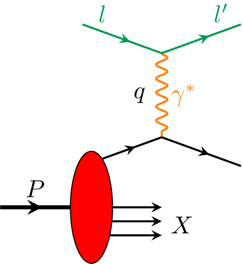
Figure 3: Deep-inelastic scattering in which partons are probed in the proton.

Shown in Fig. 3 is the DIS process in which a virtual photon with large momentum $q^{\mu}$ is absorbed by a proton of momentum $P^{\mu}$ and mass $M$. The invariant variables are $Q^{2}=-q^{\mu}q_{\mu}$ and $P\cdot q=M\nu$, and Bjorken $x_{B}=Q^{2}/(2P\cdot q)$ fixed in the scaling (or Bjorken) limit $Q^{2}\to\infty$, $P\cdot q\to\infty$. The inclusive DIS cross section can be factored into a product of leptonic and hadronic tensors, where the former is associated with the electromagnetic current of the lepton, while the latter contains all information about the electromagnetic interaction with the target proton.

To learn about the proton structure, it is best to consider the scattering in the Breit frame where

$$q^{\mu} =(0,0,0,-Q)\,,$$

$$P^{\mu} =\left(\sqrt{\frac{Q^{2}}{4x_{B}^{2}}+M^{2}},0,0,\frac{Q}{2x_{B}}\right)\,,$$ (1)

and the virtual photon has zero energy. The probe is sensitive only to the spatial structure as in non-relativistic electron scattering. However, relativity now constrains the proton to move at a large momentum $P^{z}=Q/(2x_{B})$ with boost factor $\gamma=Q/(2x_{B}M)$, which approaches $P^{z}=\infty$ in the Bjorken limit.

Feynman made intuitive assumptions about the proton structure and scattering mechanism, without QFT subtleties Feynman (1972): The proton structure at different large $P^{z}$ should be similar, and can be approximated by that at $P^{z}=\infty$, or in the IMF. The interactions between constituents (partons) are infinitely time-dilated, and the wave function configurations are frozen. The proton in high-energy scattering can be seen as being made of non-interacting partons, each with a longitudinal momentum $xP^{z}$ with $0<x<1$.

The internal structure of non-relativistic systems is independent of their overall momentum. However, relativistic systems is different as they least experience the Lorentz contraction. The structures of such systems are inextricably mixed with the overall motion, and their dependence on the external momentum is a dynamical problem. On the other hand, if the internal structure depends on a particular hadron scale $\Lambda_{\rm QCD}$, the protons at all large-momentum with $P^{z}\gg\Lambda_{\rm QCD}$ have a similar structure, corresponding to the $P^{z}\to\infty$ limit. This means that if $f(k^{z},P^{z})$ is the constituent momentum-$k^{z}$ distribution in a proton of momentum $P^{z}$, it might be analytical at $P^{z}=\infty$ and admits Taylor series expansions in $1/P^{z}$,

$$f(k^{z},P^{z})=f(x)+f_{2}(x)(\Lambda_{\rm QCD}/P^{z})^{2}+...\,,$$ (2)

where $x=k^{z}/P^{z}$. If so, one may find a large-momentum symmetry of the proton properties up to power corrections ${\cal O}(1/P^{z})$ (we omit the upper index $z$ sometimes for simplicity), and $f(x)$ is the parton distribution.

The above picture can be shown to hold in certain simple QFT models, where the dynamical frame dependence of wave functions for composite systems can be studied straightforwardly. There are many interesting examples of two-dimensional systems, for which solutions can be found. One of the much studied cases is the large $N_{c}$ QCD, also called ’t Hooft model ’t Hooft (1974), in which the bound states have a well-defined large-momentum limit. The wave functions can be expanded in $1/P$, with the corrections starting from $(1/P)^{2}$. The momenta of the constituents, $k$ and $P-k$, scale in this limit. When plotted as a function of $x=k/P$, the change in the wave function with the magnitude of the momentum can be found in Figs. 8–11 in Jia et al. (2017). This is the type of example in which Feynman’s intuition applies.

However, such a intuition fails in many 3+1 dimensional QFTs, such as QCD. When a bound state travels at increasingly large momentum, more and more high-momentum modes of a field theory are needed to build up its internal structure. Lorentz contraction indicates that the range of constituent momentum important for the structure also increases. If these high-momentum modes do not decouple effectively from the low-momentum ones, large logarithms of the form $\ln P$, will develop in the structural quantities. Hence a singularity (cut) at $P=\infty$ can exist in these theories, making $P\to\infty$ limit ill-defined and the large momentum expansion impossible. This situation is intimately related to UV properties of the theories, for which the limits of taking the UV cut-off $\Lambda_{\rm UV}\to\infty$ and $P\to\infty$ do not commute. While the physically-relevant one is $(\Lambda_{\rm UV}\gg P)\to\infty$, partons in QCD factorizations are obtained in the other limit $(\Lambda_{\rm UV}\ll P)\to\infty$ when the UV divergences are ignored. Thus one can formally write the parton distribution as

$$f(x)=\int\frac{d\lambda}{2\pi}e^{ix\lambda}\langle P^{z}=\infty|\psi^{\dagger}(z)\psi(0)|P^{z}=\infty\rangle\,,$$ (3)

where $\lambda=\lim_{P^{z}\to\infty,z\to 0}(zP^{z})$, and $\psi$ is a quantum field.

Historically, the IMF limit of field theories has been studied first at the level of diagrammatic rules for perturbation theory Weinberg (1966). It was found that taking $P\to\infty$ by ignoring the UV divergences considerably simplifies the perturbation theory rules: Many time-ordered diagrams vanish and only few have finite contributions. Moreover, scattering in this limit resembles that in non-relativistic quantum mechanics, and the wave function description becomes useful. The Fock states define the partons which have the proper kinematic support ($0<x<1$). After the limit is taken, all physical quantities are now independent of $P$, and large-momentum symmetry is exact before UV divergences are regulated. Therefore, it is the “naive” limit, $\Lambda_{\rm UV}\ll P\to\infty$, that corresponds to Feynman’s naive parton model.

In the standard QCD study of high-energy scattering, the above concept of partons as effective degrees of freedom has been used implicitly. The PDFs are defined in terms of the naive $P=\infty$ limit, and are used to match the experimental cross sections, resulting in QCD factorization theorems Collins (2011a).

I.2 Partons through Light-Front Correlators

In the literature and textbooks, parton distributions are not traditionally represented in terms of the Euclidean matrix elements as in Eq. (3). Rather, they are represented by the so-called LF correlators of quantum fields (“operator formalism”) Brodsky et al. (1998); Collins (2011a). A more explicit formulation in terms of collinear quantum fields and effective lagrangian is made in the soft-collinear effective theory (SCET) Bauer et al. (2001); Bauer and Stewart (2001); Bauer et al. (2002).

There is a physical way to see that the parton description of high-energy scattering results in the light-front correlations. Consider DIS in the rest frame of the proton, where the virtual photon has momentum

$$q^{\mu}=(\nu,0,0,-\sqrt{\nu^{2}+2x_{B}M\nu})\,.$$ (4)

In the Bjorken limit $\nu\to\infty$, although the invariant mass $Q$ of the photon goes to infinity, the photon momentum becomes actually light-like in the sense that it approaches the light front. Therefore, in inclusive DIS cross section, the separation of the two electromagnetic currents in the hadronic tensor, which is Fourier conjugate to the photon momentum, also approaches the light-cone direction.

Thus, it appears natural that all the structural physics of the proton in the IMF can also be expressed in terms of time-dependent LF correlators or correlations of quantum fields on the LF. Formally, this is simple to see if one writes

$$|P\to\infty\rangle=U(\Lambda_{\infty})|P=0\rangle\,.$$ (5)

The boost operator $U(\Lambda_{\infty})$ can be applied to the static nonlocal operators in the ordinary momentum distributions. In doing so, all static correlations become light-cone ones. The boost process is then similar to shifting the Hamiltonian evolution in quantum mechanics from Schrödinger to Heisenberg picture where time-dependence is now in the operators.

To express light-cone correlations, it is convenient to introduce two conjugate light-like (or light-cone) vectors, $p^{\mu}=(\Lambda,0,0,\Lambda)$ and $n^{\mu}=(1/2\Lambda,0,0,-1/2\Lambda)$, with the following properties, $n^{2}=p^{2}=0$, and $n\cdot p=1$, where $\Lambda$ is a parameter. Then any four-vector can be expanded as,

$$k^{\mu}=k\cdot np^{\mu}+k\cdot pn^{\mu}+k_{\perp}^{\mu}\ .$$ (6)

In particular, the momentum $P^{\mu}$ of a proton moving in the $z$-direction can be expressed as

$$P^{\mu}=p^{\mu}+(M^{2}/2)\,n^{\mu}\,,$$ (7)

where $M$ is the proton mass.

Using the above notation, one can express the unpolarized quark distribution in the proton as Collins (2011a),

$$q(x)=\frac{1}{2}\int\frac{d\lambda}{2\pi}e^{i\lambda x}\langle P|\overline{\psi}(0)\not{n}W(0,\lambda n)\psi(\lambda n)|P\rangle_{c}\ ,$$ (8)

where $\psi$ is the quark field and $W$ is a gauge-link defined as

$$W(x_{2},x_{1})=$$

$$\hskip 5.0pt{\cal P}\exp[-ig\int_{0}^{1}dt\,(x_{2}-x_{1})_{\mu}A^{\mu}(x_{1}+(x_{2}-x_{1})t)]$$ (9)

to ensure gauge invariance with ${\cal P}$ denoting the path ordering. $c$ indicates the connected contributions only, and will be suppressed in the rest of this work. It is a property of gauge theories in which the charge fields are not gauge-invariant, and the physical distributions must include a beam of collinear gauge particles. Note that the above expression is true for any momentum $P$ (a residual momentum symmetry), in particular, in the rest frame of the nucleon. The $x$-support of the above distribution is $[-1,1]$. For negative $x$, one defines the antiquark distribution with $-q(-x)\equiv\bar{q}(x)$. The above expression has been more familiar in the literature than Feynman’s original formulation of PDFs. In the single quark target, one finds $q(x)=\delta(x-1)$.

To expose the partons in the above equation, one can follow the QCD light-front quantitzation  Chang and Ma (1969); Kogut and Soper (1970); Drell and Yan (1971), suggested by Dirac in 1949 Dirac (1949). In LFQ Brodsky et al. (1998), one defines the LF coordinates,

$$\xi^{\pm}=(\xi^{0}\pm\xi^{3})/\sqrt{2}\ ,$$ (10)

where $\xi^{+}$ is the LF “time”, and $\xi^{-}$ is the LF “spatial coordinate”. And any four-vector $A^{\mu}$ will be now written as $(A^{+},A^{-},\vec{A}_{\perp})$. Dynamical degrees of freedom are defined on the $\xi^{+}=0$ plane with arbitrary $\xi^{-}$ and $\vec{\xi}_{\perp}$, with conjugate momentum $k^{+}$ and $\vec{k}_{\perp}$. Dynamics is generated by the light-cone Hamiltonian $H_{\rm LC}=P^{-}$. For a free particle with three-momentum $(k^{+},\vec{k}_{\perp})$ and mass $m$, the on-shell LF energy is $k^{-}=(\vec{k}_{\perp}^{2}+m^{2})/(2k^{+})$.

For QCD, one can define the Dirac matrices $\gamma^{\pm}=(\gamma^{0}\pm\gamma^{3})/\sqrt{2}$, and the projection operators for the quark fields as $P_{\pm}=(1/2)\gamma^{\mp}\gamma^{\pm}$, so that any $\psi$ can be decomposed into $\psi=\psi_{+}+\psi_{-}$ with $\psi_{\pm}=P_{\pm}\psi$, where $\psi_{+}$ is considered as a dynamical degree of freedom. For the gauge field, $A^{+}$ is fixed by the LF gauge $A^{+}=0$. $A_{\perp}$ are dynamical degrees of freedom. $\psi_{-}$ and $A^{-}$ are dependent variables, which can be expressed in terms of $\psi_{+}$ and $A_{\perp}$ using equations of motion Kogut and Soper (1970).

The physics of the LF correlations becomes manifest if one introduces the canonical expansion,

$$\psi_{+}(\xi^{+}=0,\xi^{-},\vec{\xi}_{\perp})=\int\frac{d^{2}k_{\perp}}{(2\pi)^{3}}\frac{dk^{+}}{2k^{+}}\sum_{\sigma}\Big{[}b_{\sigma}(k)u({k,\sigma})$$

$$\times e^{-i(k^{+}\xi^{-}-\vec{k}_{\perp}\cdot\vec{\xi}_{\perp})}+d_{\sigma}^{\dagger}(k)v({k,\sigma})e^{i(k^{+}\xi^{-}-\vec{k}_{\perp}\cdot\vec{\xi}_{\perp})}\Big{]},$$ (11)

where $b^{\dagger}(k)$ and $d^{\dagger}(k)$ ($b(k)$ and $d(k)$) are quark and antiquark creation (annihilation) operators, respectively. $\sigma$ is the light-cone helicity of the quarks which can take $+1/2$ or $-1/2$. Covariant normalization is adopted for the particle states and the creation and annihilation operators, i.e.,

$$\big{\{}b_{\sigma}(k),b_{\sigma^{\prime}}^{\dagger}(k^{\prime})\big{\}}=\big{\{}d_{\sigma}(k),d_{\sigma^{\prime}}^{\dagger}(k^{\prime})\big{\}}$$

$$=(2\pi)^{3}\delta_{\sigma\sigma^{\prime}}2k^{+}\delta(k^{+}-k^{\prime+})\delta^{(2)}(\vec{k}_{\perp}-\vec{k}_{\perp}^{\prime})\,.$$ (12)

Substituting the above expansion into Eq. (8), one finds the quark distribution as

$$q(x)=\frac{1}{2x}\sum_{\sigma}\int\frac{d^{2}{\vec{k}}_{\perp}}{(2\pi)^{3}}\langle P|b_{\sigma}^{\dagger}(x,\vec{k}_{\perp})b_{\sigma}(x,\vec{k}_{\perp})|P\rangle/\langle P|P\rangle$$ (13)

for $x>0$, and similarly for $x<0$ for which one gets the antiquark distribution. The factor $1/x$ comes from the normalization of the creation and annihilation operators. The matrix element above should be interpreted as the matrix element in a wave packet state, in the limit of a state of definite momentum Collins (2011a). This way, one recovers the physical meaning of PDFs in the LF correlator (operator) formalism.

I.3 Other Approaches to Parton Structure

Calculating the partonic structure of the hadrons from QCD has always been an important goal in hadronic physics. There have been two main approaches apart from various phenomenology and models: light-front quantization and lattice QCD. Here the authors give a very brief review on LFQ and lattice approaches that are different from the main subject of this review.

Although LFQ explicitly uses the parton degrees of freedom, it has not been very successful in practical calculations. First of all, LF perturbation theory, like the standard Hamiltonian perturbation theory, breaks Lorentz symmetry manifestly and requires a sophisticated renormalization scheme to restore it. A potential renormalization scheme must deal with the long-range correlations in the $\xi^{-}$ direction which require functional dependence on the renormalization counterterms Wilson et al. (1994). Thus LF perturbation theory has not been used for any calculations beyond one loop, except for the two-loop anomalous magnetic moment in QED Langnau and Burkardt (1993). In fact, the common wisdom of using dimensional regularization (DR) for the transverse integrals and cut-off regularization for the longitudinal one has not been proven useful for multi-loop calculations, although it has been successfully used to derive the BFKL evolution by Mueller from the quarkonium wave functions Mueller (1994a).

The enthusiasm for using LFQ in QCD is not about perturbation theory, but to solve the hadron states. Discretized LFQ was proposed in Pauli and Brodsky (1985) to make practical calculations for the bound state problems. This non-perturbative method turns out to be successful for models in 1+1 dimension, such as the Schwinger model  McCartor (1994); Harada et al. (1996), the 1+1 QCD Burkardt (1989); Srivastava and Brodsky (2001), the 1+1 $\phi^{4}$ theory Harindranath and Vary (1987) and the sine-Gordon model Burkardt (1993). For 3+1 dimensional theories, simple approximations have been considered, like the Tamm-Dancoff approximation Perry et al. (1990). For QCD itself, one again has to use severe truncations in the number of Fock states. Some recent works of this type include Vary et al. (2010); Lan et al. (2019); Jia and Vary (2019). However, to derive a fully-renormalized hamiltonian is difficult and moreover, there has been no demonstration so far that the Fock-space truncation actually converges Wilson et al. (1994). Therefore a systematic approximation for QCD bound states in LFQ has yet to be found.

Given the rapid development in lattice QCD, it is natural to use it to compute parton physics. However, simulating real-time evolution directly is numerically challenging, which runs into the so-called sign problem or more generally NP-hard problem. Over the years, a number of methods have been proposed previously to indirectly calculate the PDFs, which includes well-studied moment methods, hadronic tensor and Compton amplitude method, coordinate space factorization, etc. These approaches calculate lattice observables that can be related to the PDFs/structure functions through OPE or the dispersion relation, and thus can be used to probe certain information on the partonic structure of hadrons. However, their aims are mainly to get the lower moments of PDFs and/or segments of certain coordinate correlations, not directly in parton degrees of freedom.

The most-adopted approach on the lattice has been to calculate the moments of PDFs as the matrix elements of local operators Kronfeld and Photiadis (1985); Martinelli and Sachrajda (1987). In the moments approach, one starts with the so-called twist-two operators Christ et al. (1972),

$$O^{\mu_{1}...\mu_{n}}={\overline{\psi}}\gamma^{(\mu_{1}}iD^{\mu_{2}}...iD^{\mu_{n})}\psi-{\rm trace}$$ (14)

in the quark case, where $(\mu_{1}...\mu_{2})$ indicates that all the indices are symmetrized, the trace terms are those with at least one factor of the metric tensor $g^{\mu_{i}\mu_{j}}$ multiplied by operators of dimension $(n+2)$ with $n-2$ Lorentz indices, etc. Their matrix elements in the proton state are

$$\langle P|O^{\mu_{1}...\mu_{n}}(\mu)|P\rangle=2a_{n}(\mu)(P^{\mu_{1}}\cdots P^{\mu_{n}}\!-\!{\rm trace})\,,$$ (15)

and the PDFs are related to the local matrix elements through

$${a_{n}(\mu)} ={\int^{1}_{-1}dxx^{n-1}q(x,\mu^{2})}$$

$$=\int^{1}_{0}x^{n-1}\big{[}q(x,\mu^{2})+(-1)^{n}\bar{q}(x,\mu^{2})\big{]}$$ (16)

with $n=1,2,...$. The time-dependent correlation for the PDF in Eq. (8) is recovered by taking all the components as $+$ in Eq. (15),

$$\langle P|O^{+...+}(\mu)|P\rangle=2a_{n}(\mu)P^{+}\cdots P^{+}\,,$$ (17)

and packaging all the moments into a distribution. Likewise, for the gluon PDF, its moments are again related to the matrix elements of local operators,

$$O_{g}^{\mu_{1}...\mu_{n}}=-F^{(\mu_{1}\alpha}iD^{\mu_{2}}\cdots.iD^{\mu_{n-1}}F^{\mu_{n})}_{\ \alpha}\ ,$$ (18)

with $n=2,4,6,...$.

A large number of lattice QCD calculations of PDF moments have been done so far with various degrees of control in systematics Lin et al. (2018c), which include discretization errors, physical pion mass, finite volume effects, excited state contaminations, and proper renormalization. Most of the lattice calculations have been focused on the first and second moments, $\langle x\rangle$  Green et al. (2014); Alexandrou et al. (2017a); Bali et al. (2014), and $\langle x^{2}\rangle$Dolgov et al. (2002); Deka et al. (2009) for the unpolarized distributions, and the zero-th and first moments, $\langle 1\rangle$ Gong et al. (2017); Alexandrou et al. (2017a); Chang et al. (2018); Alexandrou et al. (2019a), and $\langle x\rangle$ Aoki et al. (2010); Abdel-Rehim et al. (2015) for the polarized distributions. However, it has been difficult to calculate higher moments, due to power divergences and rapid decay in signals. Nonetheless, moment calculations can provide a useful calibration for any comprehensive lattice approach to PDFs.

To get more information about the PDFs, it was proposed to calculate the hadronic tensor of DIS in Euclidean space, and analytically continue the result to Minkowski space Liu and Dong (1994); Liu et al. (1999); Liu (2000, 2016, 2017, 2020). Since numerical methods for analytical continuation are known to be difficult for precision control (similar to NP-hard or sign problem mentioned earlier), the approach is useful mainly for the nucleon low-lying excitations. It is very challenging to obtain parton physics this way.

A similar approach called “operator product expansion (OPE) without OPE” was suggested in Aglietti et al. (1998); Martinelli (1999), see also Dawson et al. (1998); Capitani et al. (1999a, b). The point is that the Compton amplitude in the non-dispersive region can be calculated in the Euclidean space Ji and Jung (2001). Through dispersion relation and Taylor-expansion at $\nu=P\cdot q=0$, one can extract the higher moments of structure functions from the lattice Compton amplitude. The recent works and references for parton structure from this approach can be found in Chambers et al. (2017); Hannaford-Gunn et al. (2020); Horsley et al. (2020). A similar method has been adopted for Compton amplitude with heavy-light currents Detmold and Lin (2006). This approach has been used to calculate the second moment of pion distribution amplitude Detmold et al. (2018, 2020).

The current-current correlators can also be studied through OPE in the coordinate space without momentum insertion into the currents Braun and Müller (2008). The spatial correlation at small distances can be used to calculate higher-moments of distribution amplitudes of the mesons. A number of lattice studies have been performed in Braun et al. (2015); Bali et al. (2018a, 2019). Similar strategy has been suggested more recently by Qiu et al. Ma and Qiu (2018a) for parton distributions, and has been used in lattice simulations Sufian et al. (2019, 2020). The pseudo-PDF has been proposed based on the equal-time correlation—or the quasi-PDF in Fourier space—used in LaMET Radyushkin (2017a, 2019b), and uses a coordinate-space factorization or OPE at small distance as in Braun and Müller (2008). Because of its close connection with the quasi-PDF, we will discuss comparisons of the pseudo-PDF data analysis method with that for the quasi-PDF in Sec. III.3.

There have been pioneering studies on moments of the “quasi” quark TMDPDFs on lattice  Hagler et al. (2009); Musch et al. (2011, 2012); Engelhardt et al. (2016); Yoon et al. (2017). The staple-shaped gauge link operators have been used to connect the quark fields separated in the spatial direction to simulate the moments of TMDPDF. The ratios of these moments are presumed independent of the unknown soft function and may be compared with experimental data. However, a rigorous relation of these constructions to the physical moments of TMDPDFs had not been investigated before LaMET, particularly the relationship between large momentum limit and the rapidity cutoff which is an essential ingredient of TMD physics. Comparison of this approach and LaMET will be made in Sec. V.2.

II Large-Momentum Effective Theory

As has been explained in Sec. I.1, Feynman’s partons were motivated from describing the structure of a bound state travelling at large momentum $P$. On the other hand, in QCD factorizations, they appear as effective degrees of freedoms arising in infinite momentum limit disregarding UV divergences. Reconciling these two pictures results in large-momentum effective theory (LaMET) for the parton structure of hadrons.

In this section, we start by considering the structure of the proton at finite momentum. We define the ordinary momentum distributions of the constituents, and trying to illustrate their dependence on the proton momentum. We demonstrate that the large-$P$ momentum-dependence follow a RGE, similar to the well-known RGE for partons. In Sec. II.3, we show that momentum distributions at large $P$, are related to PDFs through a matching between different orders of $P\to\infty$ and UV cut-off limits. This matching process has a standard EFT explanation: Parton physics or observables can be obtained from an effective theory in which $P\ll\Lambda_{\rm UV}$ are calculated non-perturbatively in the so-called ${\cal P}$ space Messiah (1979), after “integrating out” degrees of freedom between $P$ and $\infty$ (or ${\cal Q}=1-{\cal P}$ space) through perturbation theory. Therefore, the LaMET approach to partons is in some sense similar to lattice QCD as an EFT approach for continuum field theories, in which all active degrees of freedom (${\cal P}$ space) are bounded by $|k|\leq\pi/a$, where $a$ is lattice spacing, whereas those at $|k|\geq\pi/a$ (${\cal Q}$ space) are taken into account through perturbative coefficients and higher dimensional operators.

In Sec. II.4, we outline the formalism of LaMET for a general parton observable. The method can in principle be used also to calculate any LF correlations in terms of large momentum external states (see in particular the application to soft function in Sec. V). The strategy is also applicable for the components of the LF wave functions. Thus, LaMET offers a practical and systematic way to carry out the program of LFQ. Instead of working with the LF coordinates directly, one uses the instant form of dynamics and large momentum or boost factor $\gamma$ as a regulator for the LF divergences. In a certain sense, the quantization using tilted light-cone coordinates Lenz et al. (1991) is similar to the spirit of the LaMET approach.

At present, the only systematic approach to solve non-perturbative QCD is lattice field theory Wilson (1974). Therefore, a practical implementation of LaMET can be done through lattice calculations. It can also be done with other bound-state methods using Euclidean approaches, such as the instanton liquid model Schäfer and Shuryak (1998). While LFQ may provide an attractive physical picture for the proton, the Euclidean equal-time formulation is more practical for carrying out the calculations, and LaMET serves to bridge them.

II.1 Structure of the Proton at Finite Momentum

In relativistic theories, the internal structure of a composite system is frame-dependent (we always refer to the total momentum eigenstates), and we are interested in the properties of the proton at a momentum much larger than its rest mass.

We start from the quark momentum density in a fast-moving proton, assuming that it moves in the $z$-direction. A straightforward definition is

$$N_{P}(\vec{k})=\sum_{\sigma}\langle P|b^{\dagger}_{\sigma}(\vec{k})b_{\sigma}(\vec{k})|P\rangle/\langle P|P\rangle\ ,$$ (19)

where the quark helicity, color, and other implicit indices are summed over. This equation should be compared with the parton density in Eq. (13). To make it gauge invariant, it is convenient to consider the definition from a coordinate-space correlator,

$$N_{P,W}(\vec{k})=\int{d^{3}\xi\over{(2\pi)^{3}}}\ e^{-i\vec{k}\cdot\vec{\xi}}\langle P|\overline{\psi}(0)\gamma^{0}W(0,\vec{\xi})\psi(\vec{\xi})|P\rangle\,,$$ (20)

where the Dirac matrix $\gamma^{0}$ ensures that it is a number density. Clearly, it is a static quantity without time-dependence and can be calculated in Euclidean field theories, in contrast to Eq. (8) for partons. The gauge invariance is ensured by the Wilson line $W(0,\vec{\xi})$ between the quark fields separated by $\vec{\xi}$, which is defined in the fundamental representation of the color SU(3) group. There are infinitely many choices for the Wilson line, generating infinitely many momentum densities. For example, one can choose a straight-line link between $0$ and $\vec{\xi}$. One can also let the Wilson line run from the fields along the $z$-direction for a long distance (if not infinity) before joining them together along the transverse direction (a staple).

For its obvious connection to the PDFs, we consider a transverse-momentum integrated, longitudinal-momentum distribution,

$$N_{P}(k^{z}) =\int d^{2}\vec{k}_{\perp}\ N_{P,W}(\vec{k})$$

$$=\int{dz\over{2\pi}}e^{-ik^{z}z}\langle P|\overline{\psi}(0)\gamma^{0}W(0,z)\psi(z)|P\rangle,$$ (21)

where we ignore the question of convergence at large $|\vec{k}_{\perp}|$. Now the gauge-link $W(0,z)$ is naturally taken as a straight-line,

$$W(0,z) =\exp(-i\int^{z}_{0}A^{z^{\prime}}(z^{\prime})dz^{\prime})$$

$$=\exp(i\int^{0}_{\infty}A^{z^{\prime}}(z^{\prime})dz^{\prime})\exp(i\int^{\infty}_{z}A^{z^{\prime}}(z^{\prime})dz^{\prime})$$

$$=W^{\dagger}(\infty,0)W(\infty,z)\,,$$ (22)

where in the second line we have split the gauge link into two, going from $z$ to the infinity and coming back from the infinity to zero. We can define a “gauge-invariant” quark field

$$\Psi(\vec{\xi})=W(\infty,\vec{\xi})\psi(\vec{\xi})\ ,$$ (23)

and the above density becomes,

$$N_{P}(k^{z})=\int{dz\over{2\pi}}e^{-ik^{z}z}\langle P|\overline{\Psi}(0)\gamma^{0}\Psi(z)|P\rangle\ ,$$ (24)

where again we have not considered UV divergences. The momentum distribution defined above has been called quasi-PDF, but it is really a physical momentum distribution in a proton of momentum $P$.

In the rest frame of the proton, $N_{{P=0}}(k^{z})$ is symmetric in positive and negative $k^{z}$, probably peaks around $k^{z}=0$ and decays away as $k^{z}\to\pm\infty$. Due to the perturbative QCD effects, it decays algebraically at large $k^{z}$, instead of exponentially. Because of this property, the high moments of the distribution, $\int dk^{z}(k^{z})^{n}N_{0}(k^{z})$ with $n>0$, have the standard QFT UV divergences.

As $P$ becomes non-zero and large, the peak $N_{P}(k_{z})$ will be around $\alpha P^{z}$, where $\alpha$ is a constant of order one. The density at negative $k^{z}$ becomes smaller, but not zero. This is due to the so-called backward-moving particles from the large momentum kick in perturbation theory. For the same reason, the density at $k^{z}>P^{z}$ is not zero either.

$N_{P}(k^{z})$ has a renormalization scale dependence because the quark fields must be renormalized. One can choose DR and modified minimal subtraction ($\overline{\rm MS}$) scheme. Any other regularization scheme can be converted into this one perturbatively. For $z\neq 0$, the only renormalization necessary is the quark wave function (with anomalous dimension $\gamma_{F}$) in the $A^{z}=0$ gauge, because the linear divergence associated with the gauge link vanishes in the ${\overline{\rm MS}}$ scheme. More extensive discussions on the renormalization issue, particularly about non-perturbative renormalization, will be made in the following section.

As an example showing how the parton momentum density depends on $P$, we depict in Fig. 4 the quark wave function amplitude of a meson in the ’t Hooft model (1+1 dimensional QCD with $N_{c}\to\infty$) ’t Hooft (1974) , the square of which yields the quark momentum density. In this model, a meson of momentum $P^{\mu}$ can be built as

$$|P_{n}^{\mu}\rangle =\int\frac{dk}{2\pi|P|}\big{[}M(k-P,k)\phi_{n}^{+}(k,P)$$

$$\qquad\qquad+M^{\dagger}(k,k-P)\phi_{n}^{-}(k,P)\big{]}|0\rangle\,,$$ (25)

where $M(p,k)=\sum_{i}d^{i}_{-p}b_{k}^{i}/\sqrt{N_{c}}$, and $M^{\dagger}(p,k)=\sum_{i}b_{k}^{i\dagger}d_{-p}^{i\dagger}/\sqrt{N_{c}}$ are annihilation and creation operators for quark-antiquark pairs. The corresponding wave function amplitudes, $\phi_{n}^{+}(k,P)$ and $\phi_{n}^{-}(k,P)$, satisfy a pair of equations first derived in Bars and Green (1978).

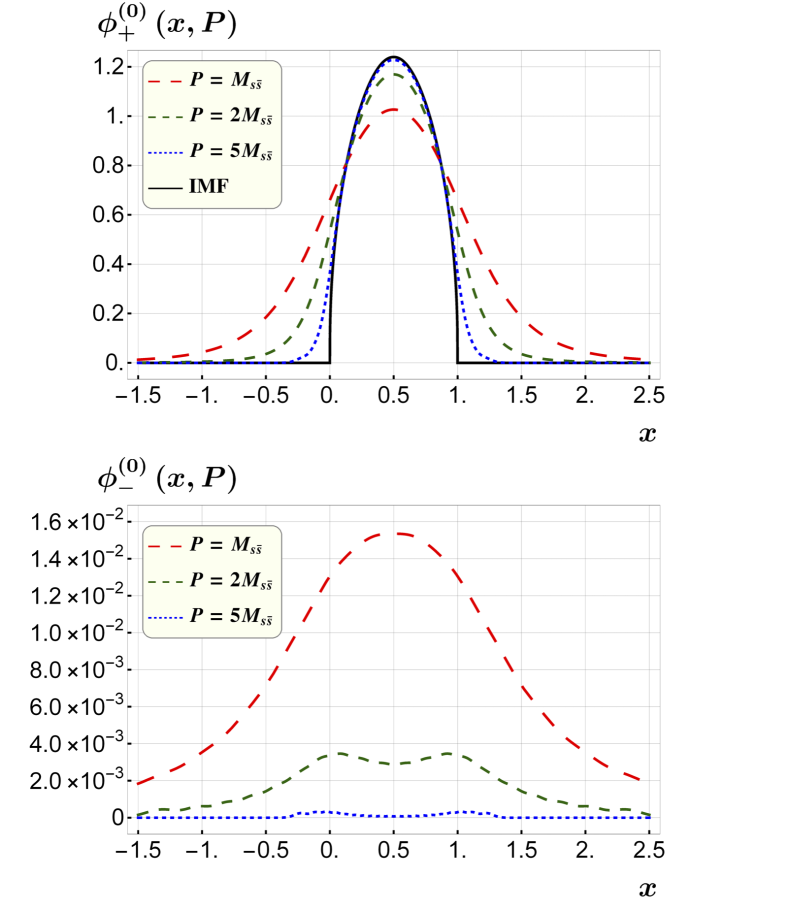
Figure 4: Wave function amplitudes of a meson in the ’t Hooft model at different external momenta Jia et al. (2017).

The meson bound state defined above has a well-defined large-momentum limit. The wave functions can be expanded in $1/P$, with the corrections starting from $(1/P)^{2}$. The momenta of the constituents, $k$ and $P-k$, scale in this limit. When plotted as a function of $x=k/P$, the change in the wave function with the magnitude of the momentum is shown in Fig. 4.

II.2 Momentum Renormalization Group

In this subsection, we consider how to calculate the external momentum $P$ dependence of physical observables discussed in the previous subsection. Clearly, the dependence is related to the boost properties of the operators under consideration, namely their commutation relations with the boost generators, $\hat{K}^{i}$. We argue that in the large momentum limit, one has a momentum RGE which is a differential equation relating properties of the system at different momenta. Momentum RGE will be, in the end, related to the renormalization properties of the observables on the LF.

Consider a generic operator $\hat{O}$, and its matrix element in a state with momentum $P$,

$$O(P)=\langle P|\hat{O}|P\rangle\ .$$ (26)

We calculate the momentum dependence by writing $|P\rangle=\exp(-i\omega(P)\hat{K})|P=0\rangle$, where $\hat{K}$ is the boost operator along the momentum direction and $\omega$ is a boost parameter depending on $P$. Taking a derivative with respect to the boost parameter gives

$$\frac{dO(P)}{dP}=i\frac{d\omega(P)}{dP}\langle P|[\hat{O},\hat{K}]|P\rangle\ .$$ (27)

The r.h.s. of the equation depends on the commutator $[\hat{O},\hat{K}]$, i.e., the boost properties of the operator. For a scalar operator, the commutation relation vanishes, and $O(P)$ is frame independent. For a vector operator, the commutation relation resembles that of an energy-momentum four-vector, and the result is the standard Lorentz transformation of a four-vector. For nonlocal operators, the commutation relation requires the elementary formula,

$$[J^{\mu\nu},\phi_{i}(x)]=i\left[l^{\mu\nu}\delta_{ij}+S^{\mu\nu}_{ij}\right]\phi_{j}(x)\ ,$$ (28)

where $l^{\mu\nu}\!=\!-i(x^{\mu}\partial^{\nu}\!-\!x^{\nu}\partial^{\mu})$ is the OAM operator and $S^{\mu\nu}$ is the intrinsic spin matrix. Thus one of the fields is now $\phi_{i}(t=\sinh\omega z,0,0,\cosh\omega z)$ which generates a time-dependent correlation function.

In the large-momentum limit, because of asymptotic freedom, the $P$-dependence is calculable in perturbation theory, and Eq. (27) simplifies. One obtains the momentum or boost RGE Ji (2014),

$$\frac{dO(P)}{dP} =\lim_{\Delta P\to 0}[O(P+\Delta P)-O(P)]/\Delta P$$ (29)

$$\xrightarrow{P\gg M}C(\alpha_{s}(P)){\otimes}O(P)+{\cal O}(M^{2}/P^{2})\ .$$ (30)

where $C(\alpha_{s}(P))$ is a perturbative expansion in the strong coupling $\alpha_{s}$. The symbol “$\otimes$” can be a simple multiplication or certain form of convolution, depending on the observable $O(P)$ studied. The proof of the above equation is non-trivial, and it can be analyzed on a case-by-case basis. There can be mixings among a set of independent operators with the same quantum numbers. The momentum RGEs are very similar to those for scale transformation or that for the coarse graining of a Hamiltonian. That the two are connected in some cases may be traced to Lorentz symmetry.

(a)

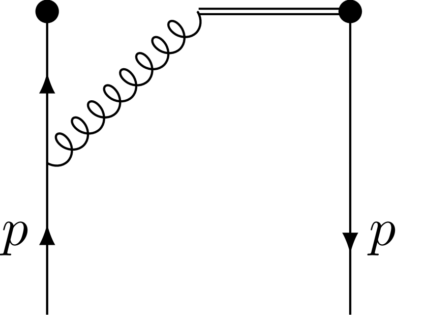
(b)

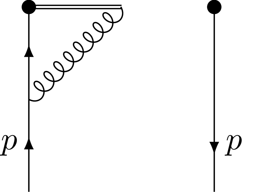
(c)

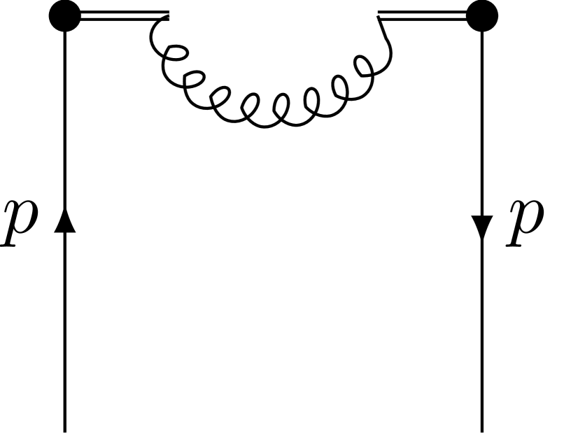
(d)

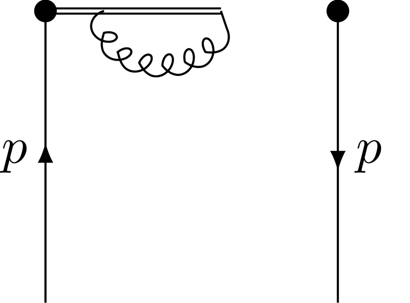
(e)

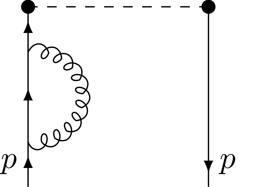
(f)

Figure 5: One-loop diagrams for the quasi-PDF in a free quark state in the Feynman gauge. The conjugate diagrams of (b), (c), (e), (f) do contribute but are not shown here.

As an example of the momentum RGE, we calculate the quark momentum distribution in a perturbative quark state using Eq. (24). Since it is gauge invariant, we can calculate it in any gauge, for example, the Feynman gauge. The one-loop diagrams in QCD are shown in Fig. 5. There are two sources of UV divergences, one is the logarithmic divergences from the vertex and self-energy diagrams, and the other is the linear divergence in the self-energy of the Wilson line. For the moment, we will use transverse momentum cut-off, $\Lambda_{\rm UV}$, as the UV regulator. Using $y=k^{z}/P^{z}$, the one-loop result reads for a large momentum quark Xiong et al. (2014),

$$\tilde{q}^{(1)}(y,P^{z},\Lambda_{\rm UV})=\frac{\alpha_{s}C_{F}}{2\pi}$$

$$\times\left\{\begin{array}[]{ll}\frac{1+y^{2}}{1-y}\ln\frac{y}{y-1}+1+\frac{\Lambda_{\rm UV}}{(1-y)^{2}P^{z}}\ ,&y>1\\ \frac{1+y^{2}}{1-y}\ln\frac{(P^{z})^{2}}{m^{2}}+\frac{1+y^{2}}{1-y}\ln\frac{4y}{1-y}\\ \,\,\,\,-\frac{4y}{1-y}+1+\frac{\Lambda_{\rm UV}}{(1-y)^{2}P^{z}}\ ,&0<y<1\\ \frac{1+y^{2}}{1-y}\ln\frac{y-1}{y}-1+\frac{\Lambda_{\rm UV}}{(1-y)^{2}P^{z}}\ ,&y<0\end{array}\right.$$ (35)

where we have ignored all power-suppressed contributions and keep the leading $P^{z}$ dependence only. There is an additional contribution of the form $\delta Z_{1}(\Lambda_{\rm UV}/P^{z})\delta(y-1)$.

The above result has several interesting features:

• The distribution does not vanish outside $[0,1]$. The radiative gluon can carry a large negative momentum fraction, resulting in a recoiling quark carrying larger momentum than the parent quark, and thus $y>1$. The same gluon can also carry a momentum larger than $P^{z}$, making the active quark have $y<0$.

• While the above effect is easy to understand perturbatively, it is surprising that a scaling contribution remains outside [0,1] in the IMF. As the proton travels faster, one might think any constituent has a momentum $k^{z}$ positive from Lorentz transformation. However, the order of limits matters because no matter how large the parent-quark momentum is, there are always quarks with much larger momentum, i.e., $k^{z}\gg P^{z}\gg\Lambda_{\rm QCD}$. In this sense, Feynman’s parton model does not describe the exact properties of the momentum distribution in a large-momentum nucleon.

• The contribution outside $[0,1]$ at one-loop is entirely perturbative because of the absence of any infrared (IR) divergence. This is no longer true at two-loop level, but the contribution depends only on the same one-loop IR physics in $[0,1]$.

• The distribution for $y$ in [0,1] has a term depending on $\ln P^{z}$. This dependence reflects that the quark substructure is resolved as a function of $P^{z}$, an interesting feature of boost. This dependence is perturbative in the sense that the derivative is IR safe,

  $$P^{z}\frac{d\tilde{q}(y,P^{z},\Lambda_{\rm UV})}{dP^{z}}$$

  $$=\frac{\alpha_{s}C_{F}}{\pi}\left[\left(\frac{1+y^{2}}{1-y}\right)_{+}-\frac{3}{2}\delta(1-y)\right]\,.$$ (36)

  Apart from the $\delta$-function term, the r.h.s. is similar to the one-loop quark splitting function in DGLAP evolution Dokshitzer (1977); Gribov and Lipatov (1972); Altarelli and Parisi (1977). Therefore one might suspect that the momentum dependence is closely related to the familiar renormalization scale evolution in the PDFs. In fact, the physics is just the other way around: It is the hadron-momentum dependence of the physical momentum distribution that generates the DGLAP evolution in the infinite-momentum limit. One can derive an all-order momentum RGE for the momentum distribution function. Momentum RGE also provides a method to sum over the large logarithms of the momentum.

• There is a singularity at $y=1$. This singularity is generated from soft-gluon radiation. Fortunately, this singularity combined with the virtual contribution yields a finite result.

• There is a linear divergence in the cut-off regulator, leading to $\Lambda_{\rm UV}/P^{z}$ term, which is absent in DR. Thus, to keep $1/(P^{z})^{2}$ power counting, it is important to work in a renormalization scheme where this term does not exist.

We can also move on to study the hadron momentum RGEs of other structural properties considered in the previous subsection. In particular, the RGE for TMD distributions will lead to the familiar rapidity RGE in the literature. We reserve these discussions to Sec. V.

II.3 Effective Field Theory Matching to PDFs

As we have seen in the previous subsection, the momentum distributions of the constituents (now called quasi-PDFs in the literature) in a proton at large $P$ are different from the PDFs or LF distributions in many ways. In particular, the momentum fraction $y$ in a physical momentum distribution is not limited to [0,1] due to backward moving particles, which is the case even in the $P\to\infty$ limit. In fact, the infinite-momentum limit is not analytical due to the presence of $\ln P$.

However, partons are effective objects arising from a different limit $\Lambda_{\rm UV}\ll P\to\infty$. There is also an important computational advantage in taking the naive limit $P\gg\Lambda_{\rm UV}$ in perturbative calculations: Feynman integrals have one fewer four-momentum. Therefore, this limit of QFTs serves as a reference system where the structure of the bound states is manifestly independent of the hadron momentum, and is similar to scale-invariant critical points at which second-order phase transitions occur in condensed matter systems. However, the theory in the naive IMF limit introduces additional UV divergences.

Therefore, the partons in QCD are very similar to the infinitely heavy quarks in HQET Manohar and Wise (2000). In certain QCD systems, heavy quarks such as the bottom quark are present, and their masses are much larger than the typical QCD scale $\Lambda_{\rm QCD}$. In this case, one might study the dependence on the heavy quark mass by expanding around $m_{Q}=\infty$. This expansion will generally produce a power series in $1/m_{Q}$. However, the limits of taking $\Lambda_{\rm UV}\to\infty$ and infinite heavy-quark mass limits are not interchangeable, due to the presence of the large logarithms $\ln m_{Q}$. In an EFT approach, one takes the $m_{Q}\to\infty$ limit first, this will result in a new theory with different UV behavior, but without the heavy-quark mass, and symmetries among very different heavy-quark systems become manifest. The renormalization of the extra UV divergences yields a RGE which can be used to resum large quark-mass logarithms.

Therefore, the momentum distribution at large-$P$ differs from the parton distributions only in the order of limits, their IR non-perturbative physics is the same. In asymptotically free theories such as QCD, differences (or discontinuities) in taking the limits of $P\gg\Lambda_{\rm UV}$ and $\Lambda_{\rm UV}\gg P\to\infty$ are perturbatively calculable, as only the high-momentum modes matter. The differences are called matching coefficients. Therefore, one is able to write down a power expansion for the momentum-dependent distribution (quasi-PDF) in terms of the PDF Xiong et al. (2014); Ma and Qiu (2018b, a); Izubuchi et al. (2018),

$$\tilde{q}(y,P^{z},\mu)\! =\!\int_{-1}^{1}\frac{dx}{|x|}C\left(\frac{y}{x},\frac{\mu}{xP^{z}}\right)q(x,\mu)$$

$$\qquad\qquad+{\cal O}\bigg{(}\frac{\Lambda_{\text{QCD}}^{2}}{(yP^{z})^{2}},\frac{\Lambda_{\text{QCD}}^{2}}{((1-y)P^{z})^{2}}\bigg{)}\,,$$ (37)

where the power correction is suppressed by the parton momentum $yP^{z}$ and the spectator momentum $(1-y)P^{z}$ Ji et al. (2020b). This expansion may be also called a factorization formula, as the quasi-PDF contains all the IR physics in the PDF, and $C$ involves only UV physics. As we will discuss extensively in the next section, this factorization formula is true to all orders in perturbation theory. The above relation allows us to calculate the LF parton physics from the momentum distribution at large $P$. Since the expansion parameter is $\Lambda_{\rm QCD}^{2}/(yP^{z})^{2}$ and $\Lambda_{\rm QCD}^{2}/((1-y)P^{z})^{2}$ , for intermediate $y$ one might not need very large $P^{z}$ to neglect the power corrections.

The above relation between the two quantities has a simple explanation in terms of the Lorentz boost: Consider the spatial correlation along $z$ shown in Fig. 6 in a large momentum state. It can be seen as approaching the LF one in the rest frame of the proton. In other words, we are using a near-LF correlation to approximate a LF correlation. Accordingly, we can invert the above equation recursively to express the PDF in terms of quasi-PDF with their differences being taken care of through the perturbative matching $\tilde{C}$ and power corrections,

$$q(x,\mu)\! =\!\int_{-\infty}^{\infty}\frac{dy}{|y|}\tilde{C}\left(\frac{x}{y},\frac{\mu}{yP^{z}}\right)\tilde{q}(y,P^{z},\mu)$$

$$\qquad\qquad+{\cal O}\bigg{(}\frac{\Lambda_{\text{QCD}}^{2}}{(xP^{z})^{2}},\frac{\Lambda_{\text{QCD}}^{2}}{((1-x)P^{z})^{2}}\bigg{)}\,.$$ (38)

The above equation has an EFT interpretation: The parton physics is calculated in an effective field theory with physical momentum scale from $0$ to $P$, whereas the physics from degrees of freedom from $P$ to $\infty$ can be integrated out to generate the perturbative coefficients $\tilde{C}$ and the high-order terms in $1/(P^{z})^{2}$. In constrast to HQET, the full QCD degrees of freedom are used in LaMET calculations. In other words, the effective Lagrangian of LaMET is the standard QCD one, while the large momentum $P$ for expansions appears only in the external states.

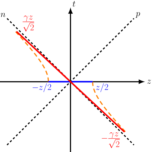
Figure 6: The line segment in the $z$-direction in the frame of a large-momentum hadron. Through Lorentz boost, it is equivalent to a line segment of length $\sim\gamma z$ close to the light-one in the hadron state of zero momentum. Here $\gamma z/\sqrt{2}$ is the length of projection of the boosted line segment to the light-cone direction $n$. Thus, we call the dimensionless variable $\lambda=zP^{z}\sim\gamma zM$ as the quasi light-cone distance.

II.4 Recipe for Parton Physics in LaMET

The principle of LaMET is to simulate the time-dependence of parton observables through external states at large momentum. Thus, we can generalize the discussions in the previous subsection to any type of physical observables for the large momentum proton, which will be generally called quasi-parton observables. Examples will be given in the later sections including transverse-momentum dependent distributions and LF wave functions.

Consider any Euclidean quasi-observable $O$ which depends on a large hadron momentum $P^{z}$ and UV cut-off $\Lambda_{\rm UV}\gg P^{z}$. Using asymptotic freedom, we can systematically expand the $P^{z}$ dependence,

$$O\Big{(}P^{z},\Lambda_{\rm UV}\Big{)}=Z\Big{(}{P^{z}\over\Lambda_{\rm UV}},{P^{z}\over\mu}\Big{)}{\otimes}o(\mu)+{\cal O}\Big{(}{\Lambda_{\rm QCD}^{2}\over(P^{z})^{2}}\Big{)}+...\ ,$$ (39)

where $\otimes$ refers to a convolution if appropriate, and $Z$ factorizes all the perturbative dependence on $P^{z}$ and does not contain any IR divergence. The quantity $o(\mu)$ is defined in a theory with $P^{z}\rightarrow\infty$, exactly as in Feynman’s parton model. In fact, $o(\mu)$ is a LF correlation containing all the IR collinear (and soft) singularities. The important point of the expansion is that it may converge at moderately large $P^{z}$, say a few GeV, allowing access to quantities needed for very large $P^{z}$ (a few TeV). One can also use the large boost-factor $\gamma=P^{z}/M$ as the expansion parameter $1/\gamma$.

Momentum dependence of the quasi-observables can be studied through momentum RGEs. Defining the anomalous dimension through

$$\gamma_{P}(\alpha_{s})=\frac{1}{Z}\frac{\partial Z}{\partial\ln P^{z}}\ ,$$ (40)

it follows that

$$\frac{\partial O(P^{z})}{\partial\ln P^{z}}=\gamma_{P}(\alpha_{s})\otimes O(P^{z})\,,$$ (41)

up to power corrections. One can resum large logarithms involving $P^{z}$ using the above equation.

When taking $P^{z}\rightarrow\infty$ first in $O(P^{z})$ before a UV regularization is imposed, one recovers from $\hat{O}$ the light-cone operator $\hat{o}$, by construction. On the other hand, the physical matrix element is calculated at a large $P^{z}$, with UV regularization such as the lattice cut-off imposed first. Thus the difference between the matrix elements of $\hat{o}$ and $\hat{O}$ is a matter of the order of limits. This is the standard set-up for an EFT. The different limits do not change the IR physics. In fact, the factorization in terms of Feynman diagrams can be proved order by order as in the renormalization program, as discussed in the following section.

The parton physics can be calculated more directly by reversing Eq. (39) to produce an EFT expansion,

$$o(\mu)=\tilde{Z}\Big{(}{P^{z}\over\Lambda_{\rm UV}},{P^{z}\over\mu}\Big{)}{\otimes}O\Big{(}P^{z},\Lambda_{\rm UV}\Big{)}+{\cal O}\Big{(}{\Lambda_{\rm QCD}^{2}\over(P^{z})^{2}}\Big{)}+...\ .$$ (42)

Thus, to compute any parton observable defined by an operator made of LF dynamical fields, $\hat{o}$, one constructs a time-independent version $\hat{O}$ which, under an infinite Lorentz boost, approaches $\hat{o}$. Then, one calculates the matrix element of $\hat{O}$ in a hadron with large momentum $P^{z}$ using whatever approach (lattice QCD is an obvious choice for the time-independent operator $\hat{O}$) and then uses Eq. (42) to systematically approximate the parton observable. Usually the matrix element of $\hat{O}$ depends on $P^{z}$ as well as all the lattice UV artifacts. In principle, the latter does not affect the EFT expansion and will be cancelled by the matching coefficient $\tilde{Z}$ and higher order terms in the expansion. However, in practical applications such as the quasi-PDF calculations, a nonperturbative renormalization is still necessary to remove all the power divergences to ensure a continuum limit.

II.5 Universality

LaMET provides a framework to systematically compute partonic observables on the LF from the properties of a large-momentum proton. However, the relationship is not one-to-one. There can be infinitely many possible Euclidean operators in the large-momentum proton which generate the same LF observable. This is because the large-momentum physical states have built-in collinear (as well as soft) parton modes, and upon acting on a Euclidean operator, they help to project out the leading LF physics. All operators projecting out the same LF physics form a universality class. Accordingly, in the operator formulation for parton physics such as SCET, one uses LF operators to project out parton physics off the external states of any momentum, including $P=0$.

The concepts such as universality class have been used in critical phenomena in condensed matter physics, where systems with different microscopic Hamiltonians can have the same scaling properties near their critical points. Critical phenomena correspond to the IR fixed points of the scale transformation, and are dominated by physics at long-distance scales. In the present case, parton physics arises from the infinite-momentum limit, $P=\infty$, which is a UV fixed point of the momentum RGEs. It is the longitudinal short distance (or large momentum) physics that is relevant at the fixed point. However, the short distance here does not mean everything is perturbative. The part that is non-perturbative characterizes the partonic structure of the proton. The critical region near $P=\infty$ acts as a filter to select only the physics that is relevant, so universality classes emerge.

In the case of unpolarized PDFs, the initial proposal in LaMET starts from the matrix element of the following operator Ji (2013),

$$O_{1}(z)=\overline{\psi}(0)\gamma^{z}W(0,z)\psi(z)\ .$$ (43)

However, one can equally start from Radyushkin (2017b); Constantinou and Panagopoulos (2017),

$$O_{2}(z)=\overline{\psi}(0)\gamma^{0}W(0,z)\psi(z)\ ,$$ (44)

and the leading contributions in the large-momentum expansion are the same. One can also consider any linear combination of the two. In Jia et al. (2018), the calculations have been done with these two operators in the ’t Hooft model, and the results have been compared at different hadron momenta. For lattice simulations, an important issue is about the operator mixing, which depends on specific choices of the operators in the universality class.

Another example of Euclidean operators for PDFs is the current-current correlators in a pure space separation,

$$O_{3}(z)=J^{\mu}(0)J^{\nu}(z)\ ,$$ (45)

where $J^{\mu}$ is, for example, an electromagnetic current. This type of correlator was first considered in Braun and Müller (2008); Bali et al. (2018b) for calculating pion DA, and recently has been suggested to calculate PDFs with generalized bilocal “currents” Ma and Qiu (2018a). When the matrix elements are calculated in the large-momentum states, $O(z)$ falls into the same universality class as the operators in Eqs. (43) and (44). Instead of using light quarks as the intermediate propagator in $O(z)$, one can have a number of other choices for LaMET applications, including scalars Aglietti et al. (1998); Abada et al. (2001) and heavy-quarks Detmold and Lin (2006). One can also similarly work with quark bilinear operators in any physical gauge which become the light-front one in the large momentum limit Gupta et al. (1993).

Another important example of universality class is the gluon helicity contribution to the spin of the proton, as we will discuss in detail in Sec. IV.4. The gluon spin operator $\vec{E}\times\vec{A}$ is gauge-dependent. However, in physical gauges where the transverse degrees of freedom are dynamical, its matrix element is the same in the large-momentum limit. Therefore, one can potentially choose different gauges to perform calculations at finite momentum on lattice, such as Coulomb gauge $\vec{\nabla}\cdot\vec{A}=0$, axial gauge $A^{z}=0$ or temporal gauge $A^{0}=0$. Different gauge choices will have different UV properties ($\ln P$) and hence different matching conditions. However, the IR part of the matrix element is the same Hatta et al. (2014).

At a practical level, it is very useful to find which operator has the fastest convergence in the LaMET expansion. The current-current correlators use the light-quark propagator to simulate the light-like Wilson line (sometimes called light-ray). The quasi-PDF approach not only starts from a quantity with clear physical meaning (a momentum distribution), but also generates the needed Wilson line simply by rotating a space-like one, shown in Fig. 6. Thus, it is plausible that the quasi-PDF will provide mathematically the fastest large-$P$ convergence than the other choices.

III Renormalization and Matching for PDFs

In this section, we consider the LaMET application to calculating the simplest collinear PDFs, which have been most extensively studied in the literature so far. Although universality allows one to extract the collinear PDFs from the matrix elements of a wide class of operators evaluated at large momentum, we will focus on physical observables closely resembling the collinear PDFs, i.e., the quark and gluon momentum distributions or the quasi-PDFs. We also discuss the coordinate-space factorization approach in which the pseudo-PDF and current-current correlators have been studied.

We mainly review the technical progress made in renormalization and matching using the quasi-PDFs. The matching can be done in principle at the bare matrix elements level, since the factorization formula like Eq. (II.3) is valid for both bare and renormalized momentum distributions. All the UV divergences in the bare quasi-PDF can be factorized into the matching coefficient $C$, and the latter automatically renormalizes the bare lattice matrix elements, so the continuum limit can be taken afterwards. However, such a matching coefficient then has to be calculated in lattice perturbation theory, which is computationally challenging and converges slowly Lepage and Mackenzie (1993). More importantly, the quasi-PDF contains linear power divergence under UV cutoff regularization due to the Wilson line self-energy Ji (2013); Xiong et al. (2014), which makes it impossible to take the continuum limit with fixed-order calculations in lattice perturbation theory. Though the latter problem can be improved by resumming the linear and possibly logarithmic divergences, it is usually preferred to nonperturbatively renormalize the quasi-PDFs on the lattice, after which a continuum limit can be taken and a perturbative matching can be done in the continuum theory. To this end, a thorough understanding of the renormalizability of Wilson-line operators defining the quasi-PDFs is required. In addition to renormalization, the applications of LaMET rely on the validity of the large-momentum factorization formula Eq. (II.3), which can be proven in perturbation theory to all orders by showing that the collinear divergences are the same in the momentum distributions and light-cone PDFs.

We begin in Sec. III.1 with the proof of multiplicative renormalizability of the Wilson-line operators that define the quasi-PDFs. We first work in the continuum theory with ${\overline{\rm MS}}$ scheme, and then generalize the conclusion to lattice theory. Next, in Sec. III.2 we outline the factorization theorem for momentum distributions to all orders in perturbation theory, and state the form of convolution between the matching coefficient and the PDF. In Sec. III.3 we show that the factorization theorem has an equivalent form in coordinate space, which can be used as an alternate route to extract PDFs from lattice matrix elements. Finally, we discuss the nonperturbative renormalization of quasi-PDFs on the lattice and their matching to the ${\overline{\rm MS}}$ PDF in Sec. III.4.

III.1 Renormalization of Nonlocal Wilson-Line Operators

The momentum distributions of the proton are defined from equal-time nonlocal Wilson line operators of the form in Eq. (21). In this subsection, we review the renormalization of these spacelike nonlocal operators (the renormalization of lightlike nonlocal operators defining the PDFs can be found in Collins and Soper (1982b); Collins (2011a)). We first discuss their renormalization in DR using an auxiliary field approach, followed by the discussion on similar gluon operators. We then consider power divergences in the momentum cutoff type of UV regularization. The conclusion is that they are all multiplicatively renormalizable with a finite number of mixings with other operators.

III.1.1 Renormalization of nonlocal quark operators

We are interested in operators of the following kind,

$$O_{\Gamma}(z)=\bar{\psi}\big{(}{z\over 2}\big{)}\Gamma W\big{(}{z\over 2},-{z\over 2}\big{)}\psi\big{(}\!-\!{z\over 2}\big{)}\ .$$ (46)

Since the Wilson line $W(z_{1},z_{2})$ is a path-ordered integral of gauge fields, it is not obvious that such operators are multiplicatively renormalizable. The renormalization of non-lightlike Wilson loops and Wilson lines has been studied in early literature Dotsenko and Vergeles (1980); Craigie and Dorn (1981), and the all-order proof of their multiplicative renormalizability was first made using diagrammatic methods in Dotsenko and Vergeles (1980); Craigie and Dorn (1981) and then the functional formalism of gauge theories in Dorn (1986). The same conclusion was conjectured to hold also for the quark bilinear operator $O_{\Gamma}(z)$, whose renormalization takes the following form Musch et al. (2011); Ishikawa et al. (2016); Chen et al. (2017),

$$O^{B}_{\Gamma}(z,\Lambda)=Z_{\psi,z}(\Lambda,\mu)e^{\delta m(\Lambda)|z|}O^{R}_{\Gamma}(z,\mu)\,,$$ (47)

where “$B$” and “$R$” stand for bare and renormalized operators respectively, and all the fields and couplings in $O^{B}_{\Gamma}(z,\Lambda)$ are bare ones which depend on the UV cutoff $\Lambda$. $\delta m(\Lambda)$ is the “mass correction” of the Wilson line, which includes all the linear power divergences of its self-energy. $Z_{\psi,z}(\Lambda,\mu)$ includes all the logarithmic divergences from wavefunction and vertex renormalizations.

An early two-loop study of the quasi-PDF in the ${\overline{\rm MS}}$ scheme indeed indicated the multiplicative renormalizability of $O_{\Gamma}(z)$ Ji and Zhang (2015). The first rigorous proof of Eq. (47) was given in the auxiliary “heavy quark” field formalism Ji et al. (2018); Green et al. (2018) which was used to prove the renormalizability of Wilson lines Samuel (1979); Gervais and Neveu (1980); Arefeva (1980); Dorn (1986). This formalism is defined by extending the QCD Lagrangian to include the auxiliary “heavy quark” fields $Q,\bar{Q}$ and their gauge interaction,

$${\cal L}={\cal L}_{\rm QCD}+\bar{Q}_{0}in_{z}\cdot D_{0}Q_{0}\,,$$ (48)

where the subscript “0” denotes bare quantities. $n_{z}^{\mu}=(0,0,0,1)$ is the direction vector of the spacelike Wilson line $W(z,0)$, $D_{0}^{\mu}=\partial^{\mu}+ig_{0}A_{0}^{\mu}$, and $Q_{0}$ is a color-triplet scalar Grassmann field in the fundamental representation of SU(3). Note that if we replace $n_{z}^{\mu}$ with the timelike vector $n_{t}^{\mu}=(1,0,0,0)$, then Eq. (48) yields the leading order HQET Lagrangian.

In the theory defined by Eq. (48), the Wilson line can be expressed as the connected two-point function of the “heavy-quark” fields,

$$\langle Q_{0}(\xi)\bar{Q}_{0}(\eta)\rangle_{Q}=S_{0}^{Q}(\xi,\eta)\,,$$ (49)

where $\xi$ and $\eta$ are space-time coordinates, and $\langle...\rangle_{Q}$ stands for integrating out the auxiliary fields. The above equation is valid up to the determinant of $in_{z}\cdot D_{0}$, which is a constant and can be absorbed into the normalization of the generating functional Mannel et al. (1992). The Green’s function $S_{0}^{Q}(\xi,\eta)$ satisfies

$$in_{z}\cdot D_{0}(\xi)\ S_{0}^{Q}(\xi,\eta)=\delta^{(4)}(\xi-\eta)\,,$$ (50)

which has the solution

$$S_{0}^{Q}(\xi,\eta)\!=\!W(\xi^{3},\eta^{3})\theta(\xi^{3}-\eta^{3})\delta(\xi^{0}-\eta^{0})\delta^{(2)}(\vec{\xi}_{\perp}-\vec{\eta}_{\perp})$$ (51)

with a proper choice of boundary condition. In this way, the Wilson-line operator $O^{B}_{\Gamma}(z)$ can be replaced by the product of two local composite operators averaged over all the “heavy-quark” field configurations Dorn (1986),

$$O^{B}_{\Gamma}(z) =\int d^{4}\xi\ \delta(\xi^{3}-z\big{)}$$

$$\quad\times\langle\bar{\psi}_{0}\big{(}{\xi\over 2}\big{)}Q_{0}\big{(}{\xi\over 2}\big{)}\Gamma\bar{Q}_{0}\big{(}\!-\!{\xi\over 2}\big{)}\psi_{0}\big{(}\!-\!{\xi\over 2}\big{)}\rangle_{Q}\,,$$ (52)

where the UV regulator is suppressed.

Consequently, the renormalization of $O^{B}_{\Gamma}(z)$ is reduced to that of the two local “heavy-to-light” currents

$$J^{B}=\bar{Q}_{0}\psi_{0}\,.$$ (53)

The renormalizability of this auxiliary field theory has been proven using the standard functional techniques for gauge theories Dorn (1986). After fixing the covariant gauge and introducing the ghost fields, the theory including the auxiliary “heavy-quark” has a residual BRST symmetry, from which one can derive the Ward-Takahashi identities to show that all the UV divergences of the Green’s functions can be subtracted with a finite number of local counterterms. In analogy, the same method has also been used to prove the all-order renormalization of HQET in perturbation theory Bagan and Gosdzinsky (1994).

According to Dorn (1986), the “heavy-quark” Lagrangian can be renormalized in a covariant gauge as

$${\cal L} ={\cal L}_{\rm QCD}[g_{0},\psi_{0},A_{0},c_{0}]+\bar{Q}_{0}in_{z}\cdot D_{0}Q_{0}$$

$$={\cal L}_{\rm QCD}[g,\psi,A,c]+{\cal L}_{\rm c.t.}[g,\psi,A,c]$$

$$+Z_{Q}\bar{Q}\left(in_{z}\cdot\partial-i\delta m\right)Q-gZ_{1}^{QQg}\bar{Q}n_{z}\cdot A_{a}t^{a}Q\,,$$ (54)

where ${\cal L}_{\rm c.t.}[g,\psi,A,c]$ are the QCD counterterms, and the bare fields and coupling are related to the renormalized ones through

$$\psi_{0}=Z_{\psi}^{1\over 2}\psi,\ A_{0}=Z_{A}^{1\over 2}A,\ Q_{0}=Z_{Q}^{1\over 2}Q,\ g_{0}=Z_{g}g\,.$$ (55)

The heavy-quark-gluon vertex renormalization constant $Z_{1}^{QQg}$ is related to $Z_{g}$ through the Slavnov-Taylor identities of the auxiliary field theory Dorn (1986),

$$Z_{g}=Z_{1}^{QQg}Z_{A}^{-{1\over 2}}Z_{Q}^{-1}\,.$$ (56)

The $i\delta m$ can be regarded as the mass correction of the “heavy quark” except that it is imaginary. For Dirac fermions, the mass correction is logarithmically divergent and proportional to the bare mass, as a result of chiral symmetry; for HQET, the mass correction of the heavy quark is proportional to the UV cutoff, i.e. linearly divergent, which is also expected for the auxiliary field here. Since the proof of renormalizability for this auxiliary field theory is carried out in the ${\overline{\rm MS}}$ scheme with DR ($d=4-2\epsilon$), all power divergences vanish, so does $\delta m$. Nevertheless, $\delta m$ may include ${\cal O}(\Lambda_{\text{QCD}})$ contributions due to the renormalon ambiguities which are known to exist in HQET Bigi et al. (1994); Beneke and Braun (1994).

Since the auxiliary field theory is renormalizable, the renormalization of the operator product in Eq. (III.1.1) amounts to the renormalizations of the two “heavy-to-light” currents. Using the standard techniques in quantum field theory Collins (1986), one can show recursively that the overall UV divergence of the insertion of $J^{B}$ into Green’s functions is absorbed into a renormalization factor $Z_{J}$ to all orders in perturbation theory,

$$J^{B} =Z_{J}J^{R}=Z_{\psi}^{1/2}Z_{Q}^{1/2}Z_{V}\ J^{R}\,,$$ (57)

where $Z_{V}$ is the vertex renormalization constant of the “heavy-to-light” current. The renormalization of heavy-to-light currents in HQET has been calculated up to three-loop order in perturbative QCD Shifman and Voloshin (1987); Politzer and Wise (1988); Ji and Musolf (1991); Chetyrkin and Grozin (2003); Broadhurst and Grozin (1991). More recently, it has been argued that the anomalous dimension of the “heavy-to-light” current is identical to that in HQET to all orders Braun et al. (2020), which is also the case for the “heavy-to-gluon” current that will be discussed below, so the renormalization factors for the spacelike and timelike Wilson line operators should be exactly the same.

Using the above results, we can show that

$$O^{B}_{\Gamma}(z)\! =Z_{J}^{2}\!\int\!d^{4}\xi\ \delta(\xi^{3}\!-\!z)\big{\langle}\bar{J}^{R}\big{(}{\xi\over 2}\big{)}\Gamma J^{R}\big{(}\!-\!{\xi\over 2}\big{)}\big{\rangle}_{Q}$$

$$=Z_{J}^{2}e^{\delta m|z|}O^{R}_{\Gamma}(z)\,,$$ (58)

where $\delta m$ arises from the determinant of $(in_{z}\cdot\partial-\delta m)$ in Eq. (III.1.1). In this way, we identify that $Z_{\psi,z}=Z_{J}^{2}$ in Eq. (47) which is independent of $\Gamma$. At one-loop order Stefanis (1984),

$$Z_{\psi,z}=1+\frac{\alpha_{s}C_{F}}{4\pi}{3\over\epsilon_{\mbox{\tiny UV}}}\,,$$ (59)

where the UV regulator $\epsilon_{\mbox{\tiny UV}}$ is to be distinguished from the IR regulator $\epsilon_{\mbox{\tiny IR}}$ in DR.

The multiplicative renormalizability of $O^{B}_{\Gamma}(z)$ has also been proven with a recursive analysis of all-order Feynman diagrams Ishikawa et al. (2017). In addition to Eq. (47), it was found that $O^{B}_{\Gamma}(z)$ does not mix with gluons or quarks of other flavors. This can also be easily understood within the auxiliary field formalism, as the flavor-changing “heavy-to-light” current does not mix with other operators Green et al. (2020).

Finally, under lattice regularization we can still use the above techniques to prove Eq. (III.1.1), where the mass correction $\delta m$ is now nonvanishing and equal to the lattice UV cutoff $1/a$ multiplied by a perturbative series in the coupling constant $\alpha_{s}$.

III.1.2 Renormalization of nonlocal gluon operators

Using the same “heavy-quark” auxiliary field formalism, it has also been proven that the Wilson-line operators for the gluon quasi-PDF are multiplicatively renormalizable Zhang et al. (2019b), which is echoed by the diagrammatical proof in Li et al. (2019).

According to LaMET, the gluon quasi-PDF can be defined as Ji (2013)

$$\tilde{g}(x,P^{z})=N\int{d\lambda\over 4\pi x(P^{z})^{2}}e^{i\lambda x}\langle P|O_{g}(z)|P\rangle\,,$$ (60)

where $N$ is a normalization factor, and

$$O^{B}_{g}(z)=g_{\perp,\mu\nu}F^{n_{1}\mu}_{0,a}\big{(}{z\over 2}\big{)}W^{ab}\big{(}{z\over 2},-{z\over 2}\big{)}F^{n_{2}\nu}_{0,b}\big{(}\!-\!{z\over 2}\big{)}$$ (61)

with $F^{n\mu}_{0,a}=n_{\rho}F^{\rho\mu}_{0,a}$ and $n_{1}^{\mu}$, $n_{2}^{\mu}$ being either $n_{z}^{\mu}$ or $n_{t}^{\mu}$. $a,b$ are color indices in the adjoint representation. The transverse metric tensor

$$g_{\perp}^{\mu\nu}=g^{\mu\nu}-n_{t}^{\mu}n_{t}^{\nu}/n_{t}^{2}-n_{z}^{\mu}n_{z}^{\nu}/n_{z}^{2}\,,$$ (62)

and $N=(n_{z}\cdot P/n_{t}\cdot P)^{(n_{1}+n_{2})\cdot n_{t}}$. For lattice implementation, $O^{B}_{g}(z)$ can also be defined as Dorn (1986); Zhang et al. (2019b)

$$O^{B}_{g}(z)\!=\!2g_{\perp}^{\mu\nu}\mbox{tr}\Big{[}F^{n_{1}}_{0,\mu}\big{(}{z\over 2}\big{)}W\!\big{(}{z\over 2},\!-\!{z\over 2}\big{)}F^{n_{2}}_{0,\nu}\big{(}\!-\!{z\over 2}\big{)}W\!\big{(}\!-\!{z\over 2},\!{z\over 2}\big{)}\Big{]}\,,$$ (63)

where $F^{\mu\nu}=F^{\mu\nu}_{a}t^{a}$ and $W$ are in the fundamental representation. Similar to Eq. (III.1.1), we can express $O^{B}_{g}(z)$ as a product of two local composite operators,

$$\tilde{O}_{g}^{B}(z) =\int d^{4}\xi\ \delta(\xi^{3}\!-\!z)$$ (64)

$$\times g_{\perp,\mu\nu}\big{\langle}F^{n_{1}\mu}_{0,a}\big{(}{\xi\over 2}\big{)}Q^{a}_{0}\big{(}{\xi\over 2}\big{)}\bar{Q}^{b}_{0}\big{(}\!-\!{\xi\over 2}\big{)}F^{n_{2}\nu}_{0,b}\big{(}\!-\!{\xi\over 2}\big{)}\big{\rangle}_{Q}$$

$$\equiv\!\int d^{4}\xi\ \delta(\xi^{3}\!-\!z)g_{\perp}^{\mu\nu}\big{\langle}J^{B}_{n_{1}\mu}\big{(}{\xi\over 2}\big{)}\bar{J}^{B}_{n_{2}\nu}\big{(}\!-\!{\xi\over 2}\big{)}\big{\rangle}_{Q}\,,$$

where the auxiliary “heavy” quark fields are in the adjoint representation, and

$$J^{\mu\nu}_{B}=F^{\mu\nu}_{0,a}Q_{0}^{a},\ \ \ \ \bar{J}^{\mu\nu}_{B}=\bar{Q}_{0}^{a}F^{\mu\nu}_{0,a}\,.$$ (65)

The renormalization of $J^{\mu\nu}_{B}$ and $\bar{J}^{\mu\nu}_{B}$ is more involved than the quark case, as they can mix with other composite operators of the same or less dimensions. In DR, BRST symmetry allows $J^{\mu\nu}_{B}$ to mix with Dorn (1986); Zhang et al. (2019b)

$$J^{\mu\nu}_{2B} \!=\!\left(n_{z}^{\nu}F^{\mu n_{z}}_{0,a}-n_{z}^{\mu}F^{\nu n_{z}}_{0,a}\right)Q_{0}^{a}/n_{z}^{2}\,,$$ (66)

$$J^{\mu\nu}_{3B} \!=\!(-in_{z}^{\mu}\!A^{\nu}_{0,a}\!+\!in_{z}^{\nu}A^{\mu}_{0,a})\big{[}(in_{z}\cdot\!D_{0}\!-\!i\delta m)Q_{0}\big{]}^{a}\!/n_{z}^{2}\,.$$ (67)

Their renormalization matrix is given by Dorn (1986)

$$\begin{pmatrix}J_{B}^{\mu\nu}\\ J_{2B}^{\mu\nu}\\ J_{3B}^{\mu\nu}\end{pmatrix} =\begin{pmatrix}Z_{11}&Z_{12}&Z_{13}\\ 0&Z_{22}&Z_{23}\\ 0&0&Z_{33}\end{pmatrix}\begin{pmatrix}J_{R}^{\mu\nu}\\ J_{2R}^{\mu\nu}\\ J_{3R}^{\mu\nu}\end{pmatrix},$$ (68)

where $J_{2B}^{\mu\nu}$ is gauge invariant while $J^{\mu\nu}_{3B}$ is gauge dependent and proportional to the equation of motion (EOM) for the auxiliary field. The Green’s functions of the EOM operator will result in a $\delta$-function,

$$(in_{z}\cdot D_{0}(\xi)-i\delta m)\langle Q_{0}(\xi)\bar{Q}_{0}(0)\rangle_{Q}=\delta^{(4)}(\xi)\,,$$ (69)

which only contributes a contact term $\delta(z)$ after integrating over the auxiliary fields. As long as $z\neq 0$, such mixing vanishes in all Green’s functions of $O^{B}_{g}(z)$, so we can ignore the mixing between $J^{\mu\nu}_{B}$ and $J^{\mu\nu}_{3B}$ in the renormalization of $O^{B}_{g}(z)$. At $z=0$, $O^{B}_{g}(z)$ becomes a local operator and is known to mix with BRST-exact and EOM operators Collins and Scalise (1994), whose renormalization can be performed in the standard way.

Note that when contracted with $n_{z}$,

$$J_{2B}^{n_{z}\mu} \!=\!J_{B}^{n_{z}\mu}=F^{n_{z}\mu}_{0,a}Q_{0}^{a}\,,$$ (70)

$$J_{3B}^{n_{z}\mu} \!=\!i\big{(}\!-\!A^{\mu,a}_{0}+{n_{z}^{\mu}\over n_{z}^{2}}n_{z}\cdot A_{0}^{a}\big{)}\big{[}(in_{z}\cdot D_{0}-i\delta m)Q_{0}\big{]}_{a}\,,$$

the $J_{B}^{n_{z}\mu}$ only mixes with the EOM operator $J_{3B}^{n_{z}\mu}$. As has been argued above, we can ignore such mixing for $z\neq 0$. Moreover, this degeneracy also leads to relations among elements in the renormalization matrix Dorn (1986),

$$Z_{11}+Z_{12}=Z_{22},\,\,\,Z_{13}=Z_{23}\,.$$ (71)

When contracted with $n_{t}$,

$$J_{B}^{n_{t}\mu} =F^{n_{t}\mu}_{0,a}Q_{0}^{a}\,,$$

$$J_{2B}^{n_{t}\mu} =n_{z}^{\mu}F_{a,0}^{n_{t}n_{z}}Q_{0}^{a}/n_{z}^{2}\,,$$

$$J_{3B}^{n_{t}\mu} =i{n_{z}^{\mu}\over n_{z}^{2}}n_{t}\cdot A_{0}^{a}\big{[}(in_{z}\cdot D_{0}-i\delta m)Q_{0}\big{]}_{a}\,.$$ (72)

As one can see, $J_{2B}^{n_{t}\mu}$ and $J_{3B}^{n_{t}\mu}$ vanish after contraction with $g_{\perp}^{\mu\nu}$, so $J_{B}^{n_{t}\mu}$ with transverse Lorentz index $\mu$ is multiplicatively renormalizable.

To summarize, for $z\neq 0$ and transverse Lorentz index $\mu$, both $J_{B}^{n_{z}\mu}$ and $J_{B}^{n_{t}\mu}$ are multiplicatively renormalizable in coordinate space, thus proving the renormalizability of the gluon Wilson-line operator $O^{B}_{g}(z)$,

$$O^{B}_{g}(z) =Z_{J}Z_{\bar{J}}\!\int\!d^{4}\xi\ \delta(\xi^{3}\!-\!z)\ g_{\perp}^{\mu\nu}\big{\langle}J_{n_{1}\mu}^{R}\big{(}{\xi\over 2}\big{)}\bar{J}_{n_{2}\nu}^{R}\big{(}\!-\!{\xi\over 2}\big{)}\big{\rangle}_{Q}$$

$$=\ e^{\delta m|z|}Z_{J}Z_{\bar{J}}\ O^{R}_{g}(z)\,,$$ (73)

where

$$J_{B}^{n_{1}\mu} =Z_{J}\ J_{R}^{n_{1}\mu}=(Z^{g}_{Q})^{1\over 2}Z_{A}^{1\over 2}Z^{g}_{V}J_{R}^{n_{1}\mu}\,,$$ (74)

$$\bar{J}_{B}^{n_{2}\nu} =Z_{\bar{J}}\ J_{R}^{n_{2}\nu}=(Z^{g}_{Q})^{1\over 2}Z_{A}^{1\over 2}Z^{g}_{\bar{V}}J_{R}^{n_{2}\mu}\,,$$ (75)

with $Z^{g}_{V}$ and $Z^{g}_{\bar{V}}$ being the renormalization constants for the vertex involving one gluon and one “heavy quark” fields. The wavefunction renormalization constant for the auxiliary “heavy quark”, $Z^{g}_{Q}$, is different from the quark case as it is in the adjoint representation.

In addition, since $J_{B}^{n_{z}\mu}$ and $J_{B}^{n_{t}\mu}$ do not mix with “heavy-to-light” quark currents due to the mismatch of quantum numbers, it implies that the nonlocal gluon Wilson-line operator does not mix with the singlet quark one under renormalization.

For the polarized gluon quasi-PDF, its definition is the same as Eq. (60), except that the gluon Wilson-line operator becomes

$$\Delta O^{B}_{g}(z)=\epsilon_{\perp,\mu\nu}F^{n_{1}\mu}_{0,a}(z)W^{ab}(z,0)F^{n_{2}\nu}_{0,b}(0)\,,$$ (76)

where $\epsilon_{\perp}^{\mu\nu}=\epsilon^{03\mu\nu}$. Since $\epsilon_{\perp}^{\mu\nu}$ only contracts with the transverse Lorentz indices, one can use the same proof for $O^{B}_{g}(z)$ to show that $\Delta O^{B}_{g}(z)$ is also multiplicatively renormalizable and does not mix with singlet quark case Zhang et al. (2019b).

Finally, one can also prove that Eq. (III.1.2) is valid under lattice regularization with $\delta m$ being linearly divergent Zhang et al. (2019b). This completes the proof of renormalizability of the gluon Wilson-line operators.

One-loop renormalization.

Now we demonstrate the above result by an explicit one-loop example. For the nonlocal Wilson-line operators to be multiplicatively renormalizable, it is important that all linear divergences associated with diagrams other than the Wilson line self-energy cancel out among themselves. To see this, a gauge symmetry preserving regularization is crucial. We use DR and keep poles around $d=3$ to identify the linear divergences Zhang et al. (2019b); Wang et al. (2019b).

The one-loop vertex correction to the “heavy-to-gluon” current is shown in Fig. 7. Each diagram contributes

$$I_{a}^{\rho\nu} =\frac{\alpha_{s}C_{A}}{\pi}\left[{1\over 4-d}{3\over 4}F_{a}^{\rho\nu}Q_{a}+{\rm finite\ terms}\right]\,,$$

$$I_{b}^{\rho\nu} =\frac{\alpha_{s}C_{A}}{\pi}\Big{[}\frac{1}{d-4}(A_{a}^{\nu}n_{z}^{\rho}-A_{a}^{\rho}n_{z}^{\nu})n_{z}\cdot\partial Q_{a}/n_{z}^{2}$$

$$+\frac{\pi\mu}{d-3}\big{(}n_{z}^{\rho}A_{a}^{\nu}-n_{z}^{\nu}A_{a}^{\rho}\big{)}Q_{a}+{\rm finite\ terms}\Big{]}\,,$$

$$I_{c}^{\rho\nu} =\frac{\alpha_{s}C_{A}}{\pi}\Big{\{}\frac{1}{d-4}\Big{[}\frac{1}{2}\big{(}F_{a}^{\rho n_{z}}n_{z}^{\nu}-F_{a}^{\nu n_{z}}n_{z}^{\rho}\big{)}Q_{a}/n_{z}^{2}$$

$$+\frac{1}{4}F_{a}^{\rho\nu}Q_{a}+\frac{1}{2}(A_{a}^{\rho}n_{z}^{\nu}-A_{a}^{\nu}n_{z}^{\rho})n_{z}\cdot\partial Q_{a}/n_{z}^{2}\Big{]}$$

$$-\frac{\pi\mu}{d-3}\big{(}n_{z}^{\rho}A_{a}^{\nu}-n_{z}^{\nu}A_{a}^{\rho}\big{)}Q_{a}+{\rm finite\ terms}\Big{\}}\,.$$ (77)

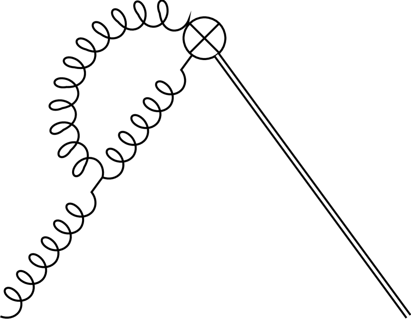
(a)

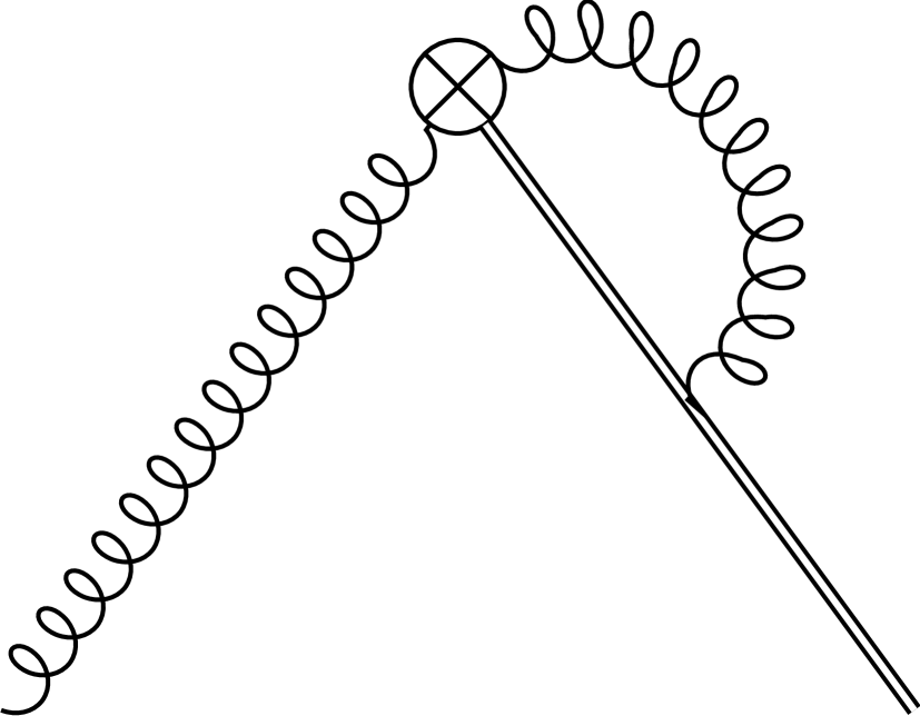
(b)

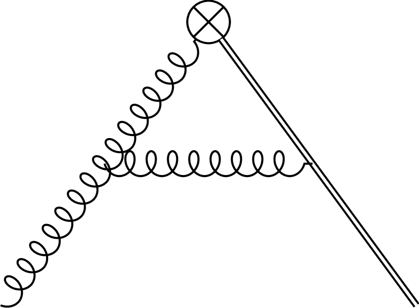
(c)

Figure 7: One-loop vertex corrections to the “heavy-to-gluon” current.

Both Fig. 7(b) and Fig. 7(c) include a linear divergence that is evident as the $\mu/(d-3)$ term, but they cancel among themselves. This guarantees that the overall UV divergence in the vertex correction is logarithmic, thus the renormalization of the “heavy-to-gluon” current is multiplicative. Combining the one-loop results in Eq. (III.1.2) and wavefunction renormalizations, we have

$$Z_{11} =1+\frac{\alpha_{s}C_{A}}{4\pi}{1\over\epsilon_{\mbox{\tiny UV}}}\,,\qquad\qquad Z_{12}=1-\frac{\alpha_{s}C_{A}}{4\pi}{1\over\epsilon_{\mbox{\tiny UV}}}\,,$$

$$Z_{13} =Z_{23}=1-\frac{\alpha_{s}C_{A}}{4\pi}{1\over\epsilon_{\mbox{\tiny UV}}}\,,\quad Z_{22}=0\,,$$ (78)

where $C_{A}=N_{c}=3$ for QCD. If we ignore the mixing to the EOM operator,

$$Z^{J^{n_{z}\nu}}_{V} =Z^{J^{\nu n_{z}}}_{V}=0\,,$$

$$Z^{J^{n_{t}i}}_{V} =Z^{J^{in_{t}}}_{V}=Z^{J^{ij}}_{V}=Z^{J^{ji}}_{V}=1+\frac{\alpha_{s}C_{A}}{4\pi}{1\over\epsilon_{\mbox{\tiny UV}}}\,,$$ (79)

where $i,j=1,2$. As a result, the one-loop current renormalization constant is

$$Z_{J^{n_{z}\nu}} =Z_{J^{\nu n_{z}}}=1+{\alpha_{s}\over 4\pi}\left({1\over 6}C_{A}-{4\over 3}n_{f}T_{F}\right){1\over\epsilon_{\mbox{\tiny UV}}}\,,$$

$$Z_{J^{n_{t}i}} =Z_{J^{in_{t}}}=Z_{J^{ij}}=Z_{J^{ji}}$$

$$=1+{\alpha_{s}\over 4\pi}\left({7\over 6}C_{A}-{4\over 3}n_{f}T_{F}\right){1\over\epsilon_{\mbox{\tiny UV}}}\,,$$ (80)

where $T_{F}=1/2$, and $n_{f}$ is the number of active quark flavors. The two-loop results can be found in Braun et al. (2020).

As one can see, the anomalous dimension of the “heavy-to-gluon” current is the same for $\mu,\nu=0,1,2$, which is due to $SO(2,1)$ (or $SO(3)$ in Euclidean space) symmetry around the $z$-axis.

III.2 Factorization of Quasi-PDFs

The key to LaMET applications for collinear parton physics is the factorization formula that relates the quasi-PDFs to light-cone PDFs Ji (2013). Here we use the perturbative properties of the matching coefficients to write the factorization form in the ${\overline{\rm MS}}$ scheme in a way consistent with a direct EFT calculations of PDFs at any given $x$ Izubuchi et al. (2018); Wang et al. (2019b)

$$q_{i}(x,\mu)\! =\!\int_{-\infty}^{\infty}\frac{dy}{|y|}\ \bigg{[}\!\sum_{j}\tilde{C}_{q_{i}q_{j}}\!\left(\frac{x}{y},\frac{\mu}{yP^{z}}\right)\tilde{q}_{j}(y,P^{z},\mu)$$ (81)

$$\qquad+\tilde{C}_{qg}\left(\frac{x}{y},\frac{\mu}{yP^{z}}\right)\tilde{g}(x,P^{z},\mu)\bigg{]}+\cdots\ ,$$

$$g(x,\mu)\! =\!\int_{-\infty}^{\infty}\frac{dy}{|y|}\ \bigg{[}\!\sum_{j}\tilde{C}_{gq}\left(\frac{x}{y},\frac{\mu}{yP^{z}}\right)\tilde{q}_{j}(y,P^{z},\mu)$$ (82)

$$\qquad+\tilde{C}_{gg}\left(\frac{x}{y},\frac{\mu}{yP^{z}}\right)\tilde{g}(y,P^{z},\mu)\bigg{]}+\cdots\,,$$

where $i,j$ runs over quark and anti-quark flavors. The “$\cdots$” term includes mass corrections whose anayltical forms have been derived to all orders of $M^{2}/(P^{z})^{2}$ Chen et al. (2016), and higher-twist contributions of order ${\cal O}\big{(}\Lambda_{\text{QCD}}^{2}/(xP^{z})^{2},\Lambda_{\text{QCD}}^{2}/((1-x)P^{z})^{2}\big{)}$ (see Eq. (II.3)). All $P^{z}$-dependence on the right hand side cancels out, just like a renormalization scale.

As we have explained in the Sec. II, the above factorization is guaranteed on the physics ground because the difference between quasi-PDFs and light-cone PDFs is the order of limits in $P^{z}\to\infty$ and $\Lambda_{\rm UV}\to\infty$, and the IR physics in both quantities must be the same. An all-order factorization proof for the quark quasi-PDF in perturbation theory was first given with a diagrammatical approach Ma and Qiu (2018b). The formula has also been derived using the operator product expansion (OPE) of nonlocal Wilson-line operators Izubuchi et al. (2018); Ma and Qiu (2018a); Wang et al. (2019b). Here we outline the diagrammatic proof similar to Ma and Qiu (2018b), showing that the collinear divergences of the quasi-PDFs do factorize and are equal to those of the light-cone PDFs. Since the collinear divergence is a concept in perturbation theory, we will show the factorization using a massless external quark state with lightlike momentum $P^{\mu}=(P^{z},0,0,P^{z})$. While the proof is only for perturbative free quark states, the factorization formulas are widely believed to be true nonperturbatively as well. We use DR to regulate both UV and collinear divergences and only consider bare quantities, since UV renormalization does not change the leading collinear divergences.

Before the analysis, we should mention that all the soft divergences cancel between the real and virtual contributions to the quasi-PDFs, as discussed in Sec. II.2, thus we only need to focus on the collinear divergences. To obtain an intuitive understanding of the structure for collinear divergences, we start from the one-loop diagram in Fig. 5(a) in the Feynman gauge. The integral reads

$$\int\frac{d^{4-2\epsilon}k}{(2\pi)^{4-2\epsilon}}\frac{{\rm tr}\big{[}\not{P}\not{k}\gamma^{z}\not{k}\big{]}\delta(k^{z}-yP^{z})}{(k^{2}+i0)^{2}((P-k)^{2}+i0)}\,.$$ (83)

The internal quark momentum is $k^{\mu}=(k^{+},k^{-},\vec{k}_{\perp})$ and the gluon momentum is $P-k$. When $k^{-}$ and $k_{\perp}=|\vec{k}_{\perp}|$ are very small, the internal quark and gluon become collinear to the external quark, i.e. $k^{\mu}\sim(k^{+},0,0_{\perp})$ and $(P-k)^{\mu}\sim(P^{+}-k^{+},0,0_{\perp})$. In this case, the denominator of the quark and gluon propagators, $(k^{2})^{2}$ and $(P-k)^{2}$, both vanish, which leads to collinear divergence. Conversely, for $k^{2}=(P-k)^{2}=0$, $k$ must be collinear to $P$ since the condition requires $k^{2}=k\cdot P=P^{2}=0$. For small $k^{-}$ and $k_{\perp}$, the $\delta$ function is dominated by the $k^{+}$ term of $k^{z}=(k^{+}-k^{-})/\sqrt{2}$ and reduces to $\sqrt{2}\delta(k^{+}-yP^{+})$. This is just the vertex which restricts $k^{+}=yP^{+}$ for the light-cone PDF, up to the factor $\sqrt{2}$. Furthermore, for collinear $k$ and $(P-k)$, the spinor trace in the numerator is dominated by the $\gamma^{+}$ part of $\gamma^{z}=(\gamma^{+}-\gamma^{-})/\sqrt{2}$, ${\rm tr}\big{[}\not{P}\not{k}\gamma^{z}\not{k}\big{]}\sim{\rm tr}\big{[}\not{P}\not{k}\gamma^{+}\not{k}\big{]}/\sqrt{2}$. Thus in the collinear region $k^{\mu}\sim(k^{+},0,0,0)$ the above integral reduces to that for the light-cone PDF:

$$\int_{\rm c}\frac{d^{4-2\epsilon}k}{(2\pi)^{4-2\epsilon}}\frac{{\rm tr}\big{[}\not{P}\not{k}\gamma^{+}\not{k}\big{]}\delta(k^{+}-yP^{+})}{(k^{2}+i0)^{2}((P-k)^{2}+i0)}\,,$$ (84)

where the subscript “c” denotes the collinear region.

The above picture naturally arises in a highly boosted hadron state where the quark is approximately onshell. Therefore, as explained in Sec. II.5, although the operator contains no light-cone information, the large-momentum external hadron state can still generate collinear divergences equivalent to those in the light-cone PDFs. By subtracting the full integral for light-cone PDF from that for the quasi-PDF, the logarithmic collinear divergence cancels, and the remaining difference is perturbative and can be absorbed into the matching kernel.

Similarly, for the vertex diagram in Fig. 5(b), the loop integral is proportional to

$$\int\frac{d^{4-2\epsilon}k}{(2\pi)^{4-2\epsilon}}\frac{1}{P^{z}-k^{z}}\frac{{\rm tr}\big{[}\not{P}\gamma^{z}\not{k}\gamma^{z}\big{]}\delta(k^{z}-yP^{z})}{(k^{2}+i0)((P-k)^{2}+i0)}\,.$$ (85)

The whole integral in the collinear region reduces to

$$\int_{\rm c}\frac{d^{4-2\epsilon}k}{(2\pi)^{4-2\epsilon}}\frac{1}{P^{+}-k^{+}}\frac{{\rm tr}\big{[}\not{P}\gamma^{+}\not{k}\gamma^{+}\big{]}\delta(k^{+}-yP^{+})}{(k^{2}+i0)((P-k)^{2}+i0)}\ ,$$ (86)

which is the corresponding integral for the light-cone PDF. One key feature of the diagram is that while the gauge link probes the $z$-component of the gluon field $A^{z}=\left(A^{+}-A^{-}\right)/\sqrt{2}$, only the $A^{+}$ component (longitudinal polarization) contributes to the leading collinear divergence. While attaching a new collinear gluon to the gauge-link induces a power suppression from the link propagator of ${\cal O}(1/P^{z})$, the $A^{+}$ component of the collinear gluon radiated from fast-moving color charges receives enhancement from Lorentz boost factor $\gamma$ that compensates for the suppression.

The above result can be generalized to all orders. Similar to the one-loop diagrams, in the leading region of collinear divergence there are an arbitrary number of longitudinally polarized $A^{+}$ gluons, which are emitted dynamically from the fast-moving state instead of being put in by hand using the lightlike gauge link, in contrast to the standard collinear PDF. The existence of the $A^{+}$ gluons clearly increases the level of complication in showing the equivalence of collinear divergences between the quasi- and light-cone PDFs. For simplification, from now on we choose to work in the light-cone gauge $A^{+}=0$ to eliminate all the $A^{+}$ gluons. Therefore, the vertex diagrams no longer contribute to the leading collinear divergence, thus making its structure much simpler.

In a general diagram, we decompose the potential leading region of the quasi-PDF into the ladder structure shown in Fig. 8. The upper two-particle-irreducible (2PI) kernel that contains the nonlocal operator defining the quasi-PDF is $H$. The 2PI kernel in the ladder is $K$. $K$ contains the upper two external quark lines but not the lower ones. The momentum flowing out of the ladders are labeled as $k_{1}$ to $k_{n}$ from bottom to top when there are $n$ 2PI kernels. We write $H$ and $K$ as matrices in spinor and momentum space. $H=H_{\alpha^{\prime}\beta^{\prime}}(yP^{z};k)$ where $k$ denotes the momentum flowing into $H$ and $K=K_{\alpha\beta;\alpha^{\prime}\beta^{\prime}}(k,k^{\prime})$ where $k$, $k^{\prime}$ are the momenta of the upper and lower external legs, respectively. Here $\alpha\beta$ and $\alpha^{\prime}\beta^{\prime}$ are the spinor indices for the upper and lower two external legs, respectively.

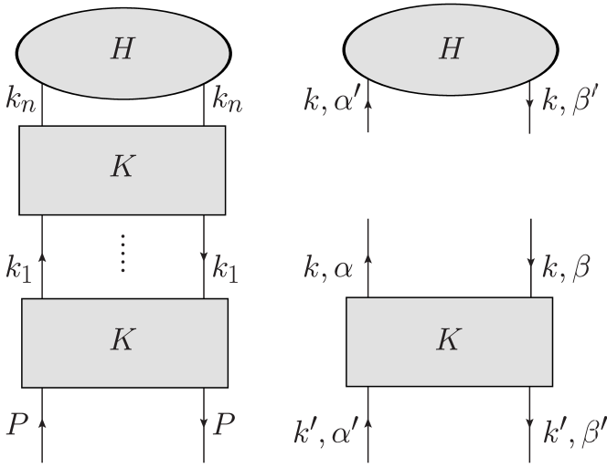
Figure 8: The ladder decomposition of the quasi-PDF (left). The upper 2PI kernel $H$ contains the operator defining the quasi-PDF, and external two legs at the bottom of the diagram is the external large $P^{z}$ state. The kernels $H$ and $K$ are shown on the right.

Following the method in Curci et al. (1980); Collins (2011a), we find that:

1. There are no collinear divergences in the upper part $H$ in the light-cone gauge.

2. If none of $k_{1},\cdots,k_{n}$ is collinear, there will be no leading collinear divergence. More generally, for the $i$’th 2PI kernel, if either of $k_{i-1}$ and $k_{i}$ is not collinear, then the sub-integrals inside the kernel are finite and it does not contribute to leading collinear divergence.

3. If $k_{i}$ is not collinear, then there are no collinear divergences for the upper part of the diagram above the $i$’th ladder.

Therefore, the collinear divergences are generated in the momentum regions $R_{i}$ in which $k_{1}$ to $k_{i}$ are collinear while $k_{i+1}$ to $k_{n}$ are not. We can construct counter terms that subtract out the collinear divergences in each of the regions $R_{i}$. For this we keep only the $+$ component of $k_{i}$ in the convergent upper part $HK^{n-i}$ as in the one-loop example, namely $k_{i}\rightarrow(k^{+}_{i},0,0_{\perp})$ in the upper part. This will clearly leave the collinear divergence unchanged. Also notice that $[HK^{n-i}]_{\alpha\beta}=H_{\alpha^{\prime}\beta^{\prime}}K^{n-i}_{\alpha^{\prime}\beta^{\prime};\alpha\beta}$ should be understood as a 4 $\times$ 4 Dirac matrix with indices $\alpha\beta$, while the lower part is $[K^{i}\not{P}]_{\alpha\beta}=K^{i}_{\alpha\beta;\alpha^{\prime}\beta^{\prime}}\not{P}_{\alpha^{\prime}\beta^{\prime}}$. In the leading region of collinear divergence, $HK^{n-i}$ and $K^{i}\not{P}$ are proportional to $\gamma^{+}$ and $\gamma^{-}$ respectively. Therefore, to obtain the leading collinear divergence, we can disentangle the spinor traces for the upper and lower parts by contracting them with $\gamma^{-}/2$ and $\gamma^{+}/2$ separately. The only communication between them is the $k^{+}$ integration. The collinear divergence is contained in the lower part

$$q^{i}(x,\epsilon_{\mbox{\tiny IR}})\!=\!\!\int\frac{dk^{-}\!d^{d-2}\!k_{\perp}}{2(2\pi)^{d}}{\rm tr}\big{[}\gamma^{+}\!K^{i}(xP^{+}\!,k^{-}\!,k_{\perp};P)\not{P}\big{]},$$ (87)

where $d=4-2\epsilon$, $k^{+}=xP^{+}$, and the subtraction for the region $R_{i}$ can be written effectively as a convolution

$$\int\frac{dx}{x}\hat{C}^{n-i}(y,x,P^{z})q^{i}(x,\epsilon_{\mbox{\tiny IR}})\ ,$$ (88)

where

$$\hat{C}^{n-i}(y,x,\!P^{z})=\frac{1}{2}{\rm tr}\left[HK^{n-i}(yP^{z};xP^{+},\!0,0_{\perp})(xP^{+})\gamma^{-}\right]$$ (89)

is the naive matching kernel. Here the $y$ dependence comes from the operator in $H$. However, the naive matching kernel still suffers from collinear sub-divergences that need to be subtracted. This can be achieved using the subtracted matching kernels $C^{n-i}(y,x)$ defined recursively in a way similar to the BPHZ relation for UV renormalization Collins (2011a). Summing over $n$ and $i$, the recursive relation leads to

$$\tilde{q}(y,P^{z},\epsilon_{\mbox{\tiny IR}}) =\sum_{n=0}^{\infty}\sum_{i=0}^{n}\int\frac{dx}{x}C^{n-i}(y,x,P^{z})q^{i}(x,\epsilon_{\mbox{\tiny IR}})$$

$$=\int\frac{dx}{x}C(y,x,P^{z})q(x,\epsilon_{\mbox{\tiny IR}})\ ,$$ (90)

where $\tilde{q}(y,P^{z},\epsilon_{\mbox{\tiny IR}})$ is the quasi-PDF, $C(y,x,P^{z})=\sum_{n=0}^{\infty}C^{n}(y,x,P^{z})$ is the all-order matching kernel and $q(x,\epsilon_{\mbox{\tiny IR}})=\sum_{i=0}q^{i}(x,\epsilon_{\mbox{\tiny IR}})$. Based on the definition of $q^{i}(x,\epsilon_{\mbox{\tiny IR}})$, it is clear that $q^{i}$ equals the light-cone PDF with $i$ 2PI kernels and $q$ is the full light-cone PDF with natural support $0<x<1$. The light-cone PDF $q(x)$ is independent of the operator defining the quasi-PDF, as it is only sensitive to the explicit form of the collinear divergence. The r.h.s. of Eq. (III.2) contains all the collinear divergences from the quasi-PDF $\tilde{q}$. Thus the matching relation for bare quantities is established. A similar matching can be written down for the renormalized quantities, where the renormalization only affects the matching kernel $C(y,x,P^{z})$. Note that the explicit solution for $C^{n-i}(y,x,P^{z})$, which leads to Eq. (II.3), can be given based on a subtraction operator defined similar to that in Collins (2011a). Besides, Eq. (III.2) can be inverted order by order in $\alpha_{s}$, thus proving Eq. (II.3), which can also be generalized to Eqs. (81) and (82).

Now we present the matching coefficient in the ${\overline{\rm MS}}$ scheme at one-loop order. The one-loop expansion of the ${\overline{\rm MS}}$ quasi- and light-cone PDFs in a free massless quark state with momentum $p^{\mu}=(p^{z},0,0,p^{z})$ are

$$\tilde{q}(y,\mu/p^{z},\epsilon_{\mbox{\tiny IR}}) =\tilde{q}^{(0)}(y)+{\alpha_{s}C_{F}\over 2\pi}\tilde{q}^{(1)}(y,\mu/p^{z},\epsilon_{\mbox{\tiny IR}})\,,$$ (91)

$$q(x,\epsilon_{\mbox{\tiny IR}}) =q^{(0)}(x)+{\alpha_{s}C_{F}\over 2\pi}q^{(1)}(x,\epsilon_{\mbox{\tiny IR}})\,.$$ (92)

At tree level, $\tilde{q}^{(0)}(y)=q^{(0)}(y)=\delta(1-y)$. At one loop, the ${\overline{\rm MS}}$ quasi-PDF and its counterterm are Izubuchi et al. (2018)

$$\tilde{q}^{(1)}(y,\mu/p^{z},\epsilon_{\mbox{\tiny IR}})$$

$$= \left\{\begin{array}[]{ll}\Big{(}{1+y^{2}\over 1-y}\ln{y\over y-1}+1+{3\over 2y}\Big{)}^{[1,\infty]}_{+(1)}-{3\over 2y}&y>1\\ \Big{(}{1+y^{2}\over 1-y}\big{[}-{1\over\epsilon_{\mbox{\tiny IR}}}-\ln{\mu^{2}\over 4(p^{z})^{2}}+\ln\big{(}y(1-y)\big{)}\big{]}&\\ \ -{y(1+y)\over 1-y}+2\sigma(1-y)\Big{)}^{[0,1]}_{+(1)}&0<y<1\\ \Big{(}-{1+y^{2}\over 1-y}\ln{-y\over 1-y}-1+{3\over 2(1-y)}\Big{)}^{[-\infty,0]}_{+(1)}&\\ \ -{3\over 2(1-y)}&y<0\end{array}\right.$$ (98)

$$+\delta(1-y)\left[{3\over 2}\ln{\mu^{2}\over 4(p^{z})^{2}}+{5+2\sigma\over 2}\right]\,,$$ (99)

$$\delta\tilde{q}^{(1)}(y,\mu/p^{z},\epsilon_{\mbox{\tiny UV}})={3\over 2\epsilon_{\mbox{\tiny UV}}}\delta(1-y)\,,$$ (100)

where $\epsilon_{\mbox{\tiny IR}}$ regulates the collinear divergence, $\sigma=0$ for $\Gamma=\gamma^{t}$ and 1 for $\Gamma=\gamma^{z}$. The plus function at $y=y_{0}$ with support in a given domain $D$ is defined as

$$\int_{D}\!dy\big{[}g(y)\big{]}_{+(y_{0})}^{D}h(y)\!=\!\int_{D}\!dy\ g(y)\left[h(y)\!-\!h(y_{0})\right]$$ (101)

with arbitrary $g(y)$ and $h(y)$. Note that the ${\overline{\rm MS}}$ renormalization of the quasi-PDF actually requires a subtle treatment of vector current conservation Izubuchi et al. (2018). We only present results in the form that is sufficient for our discussion, which differs slightly from that in Izubuchi et al. (2018) by the $\delta$-functions at $y=\pm\infty$ and from the treatment in Alexandrou et al. (2019b).

On the other hand,

$$q^{(1)}(x,\epsilon_{\mbox{\tiny IR}})={\alpha_{s}C_{F}\over 2\pi}{(-1)\over\epsilon_{\mbox{\tiny IR}}}\left({1+x^{2}\over 1-x}\right)^{[0,1]}_{+(1)}\,,$$ (102)

which is limited to the physical region as expected.

By comparing the quasi- and light-cone PDFs in Eqs. (III.2) and (102), we find that both of them have the same collinear divergence, or in other words, they share the same IR physics, thus validating the factorization formula at one-loop order. Setting $p^{z}=xP^{z}$ and plugging the one-loop results into Eq. (II.3), we extract the matching coefficient for the hadron matrix element which only depends on the perturbative scales $\mu$ and $P^{z}$,

$$C^{{\overline{\rm MS}}}\left(y,{\mu\over xP^{z}}\right) =\delta\left(1-y\right)+{\alpha_{s}C_{F}\over 2\pi}\left[\tilde{q}^{(1)}\left(y,{\mu\over xP^{z}},\epsilon_{\mbox{\tiny IR}}\right)\right.$$

$$\qquad\left.-q^{(1)}(y,\epsilon_{\mbox{\tiny IR}})\right]\,.$$ (103)

The complete one-loop matching coefficients in Eq. (II.3) in the transverse-momentum cutoff and ${\overline{\rm MS}}$ schemes can be found in Wang et al. (2018); Wang and Zhao (2018); Wang et al. (2019b). The two-loop results were obtained recently in Chen et al. (2020c, a, b); Li et al. (2020).

III.3 Coordinate-Space Factorization of Bilinear Operators

Although the LaMET application to PDFs concerns the expansion of momentum densities in the $P^{z}\to\infty$ limit, lattice QCD calculations actually start from computing coordinate-space correlations, for example,

$$\tilde{h}(z,P^{z})={1\over N_{\Gamma}}\langle P^{z}|O_{\Gamma}(z)|P^{z}\rangle\,,$$ (104)

at all $z$ and do Fourier transform with respect to $\lambda=zP^{z}$ at a fixed $P^{z}$. Here the normalization factor $N_{\Gamma}=2P^{z}$ for $\Gamma=\gamma^{z}$ and $N_{\Gamma}=2P^{t}$ for $\Gamma=\gamma^{t}$. The $\tilde{h}(z,P^{z})$ is a function of two independent variables $z$ and $P^{z}$, and in LaMET analysis the relevant combinations are quasi-LF distance $\lambda$ (see Fig. 6) and $P^{z}$, hence $\tilde{h}(\lambda,P^{z})$ will be called quasi-LF correlation, which is distinguished from the LF correlation $h(\lambda,\mu)$ below.

The coordinate-space factorization approach in Braun et al. (1995) has been suggested as an alternative way to extract the PDFs from $\tilde{h}(z,P^{z})$ Radyushkin (2017a); Orginos et al. (2017); Radyushkin (2019a), which is closely related to the OPE. Instead of working with variables $\lambda$ and $P^{z}$, one may consider $\tilde{h}$ as a function of $\lambda$ and $z^{2}$, i.e., $\tilde{h}(\lambda,z^{2})$. The Fourier transform of $\tilde{h}(\lambda,z^{2})$ with respect to $\lambda$ is no longer the momentum distribution of the proton at a fixed momentum. Instead, it is called a pseudo-distribution Radyushkin (2017a). At small $|z|\ll\Lambda^{-1}_{\rm QCD}$, $\tilde{h}(\lambda,z^{2})$ can be factorized into the light-cone correlation Radyushkin (2018a); Izubuchi et al. (2018),

$$\tilde{h}(\lambda,z^{2}\mu^{2})=\int_{-1}^{1}d\alpha\ \mathcal{C}(\alpha,z^{2}\mu^{2})\ h(\alpha\lambda,\mu)+...\,,$$ (105)

where $...$ are the power corrections in $z^{2}\Lambda^{2}_{\rm QCD}$, and the matching coefficient $\mathcal{C}$ is related to $C$ in Eq. (II.3) by

$$C\left(\eta,{\mu\over xP^{z}}\right)\!=\!\int{d\lambda\over 2\pi}\ e^{i\eta\lambda}\int_{-1}^{1}\!\!d\alpha\>e^{-i\lambda\alpha}\>\mathcal{C}\left(\alpha,{\mu^{2}\lambda^{2}\over(xP^{z})^{2}}\right)\,.$$ (106)

To illustrate the connection between the above factorization in Eq. (105) and OPE, let us take the non-singlet quark case as an example Izubuchi et al. (2018); Wang et al. (2019b). In the ${\overline{\rm MS}}$ scheme, the renormalized $O_{\gamma^{\mu_{0}}}(z,\mu)$ can be expanded in terms of local gauge-invariant twist-2 operators as $z^{2}\to 0$,

$$O_{\gamma^{\mu_{0}}}(z,\mu) =\sum_{n=0}^{\infty}\Big{[}C_{n}({\mu}^{2}z^{2})\frac{(iz)^{n}}{n!}(n_{z})_{\mu_{1}}\cdots(n_{z})_{\mu_{n}}$$

$$\qquad\times O^{\mu_{0}\mu_{1}\cdots\mu_{n}}(\mu)+\text{higher-twist}\Big{]}\,,$$ (107)

where $\mu_{0}\!=\!0$ or $3$, $C_{n}\!=\!1+{\cal O}(\alpha_{s})$ is the Wilson coefficient, and $O^{\mu_{0}\mu_{1}\cdots\mu_{n}}(\mu)$ is the twist-two operator in Eq. (14).

Using the hadron matrix elements in Eq. (15) and their relation to the light-cone PDF in Eq. (16), we write down the small-$|z|$ expansion of the hadron matrix element of $O_{\gamma^{\mu_{0}}}(z,\mu)$ Izubuchi et al. (2018),

$$\tilde{h}(\lambda,z^{2}\mu^{2}) =\langle P|O_{\gamma^{\mu_{0}}}(z,\mu)|P\rangle/(2P^{\mu_{0}})$$

$$=\sum_{n=0}^{\infty}\ C_{n}(z^{2}\mu^{2}){(-i\lambda)^{n}\over n!}\left[1+{\cal O}\big{(}{M^{2}\over(P^{z})^{2}}\big{)}\right]$$

$$\quad\times\int_{-1}^{1}dx\ x^{n}q(x,\mu)+{\cal O}\left(z^{2}\Lambda_{\text{QCD}}^{2}\right)\,,$$ (108)

where the ${\cal O}\left(M^{2}/(P^{z})^{2}\right)$ term comes from the kinematic trace contribution and the ${\cal O}\left(z^{2}\Lambda_{\text{QCD}}^{2}\right)$ term from higher-twist. The Wilson coefficients $C_{n}(z^{2}\mu^{2})$ have been calculated at one-loop Izubuchi et al. (2018) and two-loop Li et al. (2020) orders. Comparing the above equation with Eq. (105), we identify

$$\mathcal{C}(\alpha,{\mu}^{2}z^{2})\equiv\int\!\frac{d\lambda}{2\pi}\,e^{i\lambda\alpha}\sum_{n}C_{n}({\mu}^{2}z^{2})\frac{(-i\lambda)^{n}}{n!}\,.$$ (109)

Since $z^{2}$ is fixed in $\mathcal{C}(\alpha,{\mu}^{2}z^{2})$, the integration in Eq. (109) is actually over $P^{z}$ from $-\infty$ to $+\infty$. $\mathcal{C}(\alpha,z^{2}\mu^{2})$ has support $-1\leq\alpha\leq 1$, and its one-loop result is

$${\cal C}(\alpha,z^{2}\mu^{2})$$ (110)

$$= \left[1+{\alpha_{s}C_{F}\over 2\pi}\left({3\over 2}\ln{z^{2}\mu^{2}e^{2\gamma_{E}}\over 4}+{3\over 2}\right)\right]\delta(1-\alpha)$$

$$+{\alpha_{s}C_{F}\over 2\pi}\left\{\left({1+\alpha^{2}\over 1-\alpha}\right)^{[0,1]}_{+(1)}\left[-\ln{z^{2}\mu^{2}e^{2\gamma_{E}}\over 4}-1\right]\right.$$

$$\left.-\left(4\ln(1-\alpha)\over 1-\alpha\right)^{[0,1]}_{+(1)}\!+\!2(1+\sigma)(1-\alpha)\right\}\!\theta(\alpha)\theta(1-\alpha)\,,$$

which was also calculated and further studied in Ji et al. (2017b); Radyushkin (2018a, b); Zhang et al. (2018); Li et al. (2020). One can check that the above result is indeed related to one-loop momentum-space matching by Eq. (106). Since we are interested in the relation between the quasi-LF correlation with the matrix element of the light-ray operator $O_{\gamma^{+}}(\lambda n)$, Eq. (105) can also be obtained by using the light-ray operator expansion in Balitsky and Braun (1989); Braun et al. (1995); Braun and Müller (2008).

Using OPE or short-distance expansion, the exact factorization formula for the gluon and singlet quark quasi-PDFs, which includes their mixings, has also been derived in coordinate space and studied at one-loop order Wang et al. (2019b); Balitsky et al. (2019).

It is easy to see that the limits $P^{z}\to\infty$ in LaMET expansion and $z\to 0$ in coordinate-space factorization, keeping finite $\lambda=zP^{z}$, are equivalent. However, in practical lattice QCD calculations, one is limited by the largest momentum $P^{z}_{\rm max}$ in a specific setup, and the two approaches start to differ.

In LaMET systematic approximation, one should calculate $\tilde{h}(z,P^{z}_{\rm max})$ with all possible $z$ or $\lambda$, but in practice the largest $\lambda_{\rm max}=z_{\rm max}P^{z}_{\rm max}$ is limited by the lattice volume as well as data quality at large $z$. Due to QCD confinement, $\tilde{h}(z,P^{z}_{\rm max})$ has a correlation length $\sim 1/\Lambda_{\rm QCD}$, leading to an exponential decay at large $z$ Ji et al. (2020b). Therefore, if $z_{\rm max}$ is sufficiently large (e.g., the proton size $\sim 1$ fm) for $\tilde{h}(z,P^{z}_{\rm max})$ to fall to almost zero, then the truncated Fourier transform of $\tilde{h}(z,P^{z}_{\rm max})$ should converge quickly, and the truncation effects mainly affect results at small $x\lesssim 1/\lambda_{\rm max}$. If $\tilde{h}(z,P^{z}_{\rm max})$ exhibits exponential decay but still has a nonzero value at $z_{\rm max}$, then one can perform a physically motivated extrapolation beyond $z_{\rm max}$ Ji et al. (2020b) to do the Fourier transform, which removes the unphysical oscillation from truncation and only affects the small-$x$ region. In the momentum space, one can use LaMET expansion to calculate the PDF point by point in $x$ with systematic error controlled by $\Lambda_{\rm QCD}^{2}/(xP^{z}_{\rm max})^{2}$ and $\Lambda_{\rm QCD}^{2}/((1-x)P^{z}_{\rm max})^{2}$, which gives the prediction for a cetain region of $x$, $[x_{\rm min},x_{\rm max}]$, with a target error.

In coordinate-space factorization, one expands $\tilde{h}(\lambda,z^{2})$ in $z^{2}\Lambda^{2}_{\rm QCD}$. For the factorization formula to be valid, $z$ must remain in the perturbative region. For example, an estimate in Ji et al. (2020b) gives $z_{\rm max}\sim 0.3$–$0.4$ fm. Although there have been observations that forming ratios of $\tilde{h}(\lambda,z^{2})$ may cancel the higher-twist contributions at $z>0.4$ fm Orginos et al. (2017), this cancellation needs be quantified for precision calculations. With a finite range of quasi-LF correlations, the PDFs can be extracted through modelling the $x$-dependence or more advanced techniques such as Bayesian analysis Bringewatt et al. (2020) or neural network Karpie et al. (2019); Cichy et al. (2019); Del Debbio et al. (2020a), which is similar to extracting the PDFs from experimental data Ma and Qiu (2018a), although quantifying the systematic error from fitting can be challenging. The coordinate-space factorization can also provide the extraction of the lowest moments of PDFs Karpie et al. (2018); Shugert et al. (2020); Joó et al. (2020); Gao et al. (2020), where the main systematic error is controlled by $z^{2}\Lambda_{\rm QCD}^{2}$.

So far, there have been very limited studies about the comparison between quasi- and pseudo-PDF analysis  Bhat et al. (2020); Alexandrou et al. (2020c). It remains to be seen how systematic errors in the two strategies are compared and contrasted.

III.4 Nonperturbative Renormalization and Matching

The multiplicative renormalizability of the nonlocal Wilson-line operators for quasi-PDFs allows a nonperturbative renormalization on the lattice, after which the continuum limit can be taken. This is an important step in the application of LaMET. One way of doing so is to perform a mass subtraction of the Wilson line first Musch et al. (2011); Ishikawa et al. (2016); Chen et al. (2017); Zhang et al. (2017); Green et al. (2018, 2020), and then renormalize the remnant UV divergences with lattice perturbation theory or other nonperturbative schemes. Another scheme which has gained more popularity in recent years is the regularization-independent momentum subtraction (RI/MOM) scheme Constantinou and Panagopoulos (2017); Stewart and Zhao (2018); Alexandrou et al. (2017b); Chen et al. (2018); Liu et al. (2020). In the coordinate space approach where $|z|\ll\Lambda_{\rm QCD}^{-1}$, the ratios of quasi-LF correlations in different states Radyushkin (2017a); Orginos et al. (2017); Braun et al. (2019); Li et al. (2020) have also been proposed as a renormalization scheme. At large $z$, the RI/MOM and ratio schemes introduce extra nonperturbative effects at different levels, which may distort the IR property of the original quasi-LF correlations. Due to the suppression of long-range contributions by large $P^{z}$ in the Fourier transform, this nonperturbative contamination mainly affects the end-point region in $x$-space, while the existing LaMET calculations with RI/MOM scheme at moderate $x$, for example in Alexandrou et al. (2018b); Lin et al. (2018a), suffers less from such systematics. Nevertheless, the above complication can be avoided by switching to the hybrid scheme Ji et al. (2020b) where one utilizes the advantages of different schemes at short and large distances. In the following, we discuss the above schemes in order, with a particular focus on the hybrid renormalization scheme.

Before we proceed, it should be noted that the current-current correlators in Detmold and Lin (2006); Braun and Müller (2008); Ma and Qiu (2018a) do not need or have simple renormalization on the lattice, though it might be more costly to simulate them. Besides, there is another distinct method based on a redefinition of the quasi-PDF with smeared fermion and gauge fields via the gradient flow Monahan and Orginos (2017). The smeared quasi-PDF is free from UV divergences and remains finite in the continuum limit, which can be perturbatively matched onto the PDF Monahan (2018b). Nevertheless, this method awaits to be implemented on the lattice.

III.4.1 Wilson-line mass-subtraction scheme

Since the mass correction $\delta m$ includes all the linear UV divergences, it is highly favored to nonperturbatively subtract it from the quasi-PDFs. It is well known that the Wilson line renormalization is related to the additive renormalization of the static quark-antiquark potential, i.e., $\delta m$, especially in the context of finite temperature field theory. For a rectangle-shaped Wilson loop of dimension $L\times T$ in the spatial and temporal directions, its vacuum expectation value for large $T$ scales as

$$\lim_{T\to\infty}W(L,T)=c(L)e^{-V(L)T}\,.$$ (111)

The renormalized static potential is

$$V^{R}(L)=V(L)+2\delta m\,,$$ (112)

and $\delta m$ can be fixed by imposing the condition $V^{R}(L_{0})=0$ for a particular value of $L_{0}$. Alternatively, one can also fit $\delta m$ from the famous string potential model,

$$V(L)=\sigma L-{\pi\over 12L}-2\delta m\,.$$ (113)

Apart from using the static potential to determine $\delta m$, it was also proposed to calculate this quantity in the auxiliary “heavy quark” field theory with the following condition Green et al. (2018),

$$\delta m={d\over dz}\ln{\rm Tr}\big{\langle}Q(x+zn_{z})\bar{Q}(x)\big{\rangle}_{{\rm QCD}+Q}\Big{|}_{z=z_{0}}\,.$$ (114)

Other suggestions have also been made for a nonperturbative calculation of $\delta m$ Ji et al. (2020b). For example, one can investigate the asymptotic large-$z$ behavior of the hadron matrix element or the single quark Green’s function, of the vacuum expectation value of $O_{\Gamma}(z,a)$ in a fixed gauge. The $\delta m$ calculated from all these matrix elements will have the following dependence on the lattice spacing $a$,

$$\delta m=m_{-1}(a)/a+m_{0}\ ,$$ (115)

where $m_{-1}$(a) is the coefficient of the power divergence which is independent of the specific matrix element, while $m_{0}~{}\sim O(\Lambda_{\rm QCD})$ is finite and depends on the external state. The determination of $m_{0}$ can be rather nontrivial, and in practical calculations one could adopt a fine-tuning method, such as that for the Wilson-fermion mass, to find the critical value of $m_{0}$ at which the final result converges fastest in the large $P^{z}$ limit.

After the Wilson-line mass subtraction, there are still logarithmic UV divergences in $O_{\Gamma}(z,a)$. One can use lattice perturbation theory to match $\delta m$-subtracted $O_{\Gamma}(z,a)$ to the ${\overline{\rm MS}}$ scheme Ishikawa et al. (2016); Xiong et al. (2017); Constantinou and Panagopoulos (2017), but the convergence still needs to be examined at higher orders. In Green et al. (2018, 2020), the logarithmic divergences were nonperturbatively renormalized with RI/MOM-like schemes.

The Wilson-line mass-subtraction has been implemented on the lattice in Musch et al. (2011); Zhang et al. (2017); Green et al. (2018); Zhang et al. (2019c); Alexandrou et al. (2020c).

III.4.2 RI/MOM scheme

The RI/MOM scheme has been widely used in lattice QCD for the renormalization of local composite quark operators that are free from power-divergent mixings  Martinelli et al. (1995). It is essentially a momentum subtraction scheme in QFT and can be nonperturbatively implemented on the lattice. For an arbitrary composite quark bilinear operator $O^{B}$ that is multiplicatively renormalized as $O^{B}=Z_{O}O^{R}$, the RI/MOM scheme is defined by imposing the following condition on its off-shell quark matrix element at a subtraction scale $\mu_{\tiny R}$,

$$Z^{-1}_{O}\langle p|O^{B}|p\rangle\Big{|}_{p^{2}=-\mu_{\tiny R}^{2}}=\langle p|O|p\rangle_{\rm tree}\,.$$ (116)

where the subscript “tree” means the tree-level matrix element in perturbation theory. If $\mu_{\tiny R}\gg\Lambda_{\rm QCD}$, $Z_{O}$ defined in Eq. (116) is in the perturbative region, and we can convert it to the ${\overline{\rm MS}}$ scheme order by order in perturbation theory. In this sense, $Z_{O}$ is not literally nonperturbative, but an all-order calculable quantity.

Since the nonlocal quark bilinear operator $O_{\Gamma}(z)$ has been proven to be multiplicatively renormalizable in the coordinate space, one can also renormalize it in the RI/MOM scheme and then match the result to PDF in the ${\overline{\rm MS}}$ scheme Constantinou and Panagopoulos (2017); Stewart and Zhao (2018). On the lattice, the off-shell matrix element of an operator is defined from its amputated Green’s function, or vertex function, with off-shell quarks. For the nonlocal Wilson-line operator, the latter is

$$\Lambda^{\Gamma}_{0}(z,a,p)\equiv\left[S^{-1}_{0}(p,a)\right]^{\dagger}\sum_{x,y}e^{ip\cdot(x-y)}$$

$$\ \ \ \times\!\big{\langle}0\big{|}T\bigl{[}\psi_{0}(x,a)O^{B}_{\Gamma}(z,a)\bar{\psi}_{0}(y,a)\bigr{]}\big{|}0\big{\rangle}S^{-1}_{0}(p,a)\,,$$ (117)

where $S_{0}(p,a)$ is the bare quark propagator, and the external momentum $p$ is Euclidean on the lattice. Since Green’s functions are not gauge invariant, one needs to fix a gauge (usually Landau gauge $\partial\cdot A=0$ is chosen), and the gauge dependence is expected to be canceled by the matching or scheme conversion order by order in perturbation theory.

After including the quark wavefunction renormalization $Z_{q}$, which can be determined independently on the lattice Martinelli et al. (1995), Eq. (116) is revised as

$$Z_{q}Z^{-1}_{O_{\Gamma}}\Lambda^{\Gamma}_{0}(z,a,p)\Big{|}_{p=p_{\tiny R}}=\Lambda^{\Gamma}_{\rm tree}(z,a,p)=\Gamma e^{ip_{\tiny R}\cdot z}\,.$$ (118)

Since $O_{\Gamma}(z,a)$ is not $O(4)$ covariant, one needs to define the RI/MOM scheme with two scales, one is $\mu_{\tiny R}=|p_{R}|$, and the other $p_{\tiny R}^{z}$. For convenience we simply denote them as $p=p_{\tiny R}$. To work in the perturbative region and control the lattice discretization effects that are of order ${\cal O}\big{(}a^{2}\mu_{\tiny R}^{2},a^{2}(p_{\tiny R}^{z})^{2}\big{)}$, one must work in the window $\Lambda_{\rm QCD}\ll\mu_{\tiny R}\ll a^{-1}$, $p_{\tiny R}^{z}\ll a^{-1}$, which is attainable if the lattice spacing is small enough.

Since the quarks are off-shell, also finite mixings with the EOM operators can appear. As a result, Eq. (118) in general cannot be satisfied as a matrix equation. Instead, one usually needs a projection operator ${\cal P}$ to define the off-shell matrix elements, i.e.

$$\langle p|O^{B}_{\Gamma}|p\rangle={\rm tr}\big{[}\Lambda^{\Gamma}_{0}(z,a,p){\cal P}\big{]}\,,$$ (119)

so as to calculate the renormalization factor $Z_{O_{\Gamma}}$.

Then, the bare hadron matrix element $\tilde{h}_{B}(z,P^{z},a)$ can be renormalized in coordinate space as

$$\tilde{h}_{R}(z,P^{z},p_{\tiny R}^{z},\mu_{\tiny R},a)=Z^{-1}_{O}(z,p_{\tiny R}^{z},\mu_{\tiny R},a)\tilde{h}_{B}(z,P^{z},a)\,,$$ (120)

In the continuum limit, the renormalized matrix element is independent of the UV regulator, so we should obtain the same result in DR under RI/MOM scheme, i.e.,

$$\tilde{h}_{R}(z,P^{z},p_{\tiny R}^{z},\mu_{\tiny R})=\lim_{a\to 0}\tilde{h}_{R}(z,P^{z},p_{\tiny R}^{z},\mu_{\tiny R},a)$$

$$\qquad=\lim_{\epsilon\to 0}Z^{-1}_{O}(z,p_{\tiny R}^{z},\mu_{\tiny R},\epsilon)\tilde{h}_{B}(z,P^{z},\epsilon)\,,$$ (121)

which allows us to compute the matching coefficients in continuum perturbation theory. Note that $\delta m$ vanishes in $Z_{O}$ due to the use of DR.

By Fourier transforming the above renormalized matrix element to momentum space, one can then work out the RI/MOM matching coefficient for the quasi-PDFs Stewart and Zhao (2018). The one-loop matching coefficient for different spin structures has been obtained in Stewart and Zhao (2018); Liu et al. (2020, 2018), and the two-loop result for the unpolarized case can be found in Chen et al. (2020b). Alternatively, one can also first convert the RI/MOM matrix element to the ${\overline{\rm MS}}$ or modified ${\overline{\rm MS}}$ schemes Constantinou and Panagopoulos (2017); Alexandrou et al. (2019b), and then do the Fourier transform and momentum-space matching.

III.4.3 Ratio scheme

In the coordinate-space factorization, $|z|\ll\Lambda^{-1}_{\rm QCD}$ must be small, whereas $P^{z}$ can be of any value. In this case, the ratio scheme in Radyushkin (2017a); Orginos et al. (2017) can be an effective choice for lattice renormalization. Consider the ratio

$$\tilde{h}(\lambda,z^{2},a)/\tilde{h}(0,z^{2},a)\,,$$ (122)

where the denominator is a nonperturbative matrix element at $P^{z}=0$. Since $\tilde{h}(\lambda,z^{2},a)$ and $\tilde{h}(0,z^{2},a)$ calculated from the same lattice ensemble are correlated with each other, the error in the ratio can be reduced. Besides, the ratio does not need further renormalization on the lattice, so one can directly take the continuum limit

$$\lim_{a\to 0}\frac{\tilde{h}(\lambda,z^{2},a)}{\tilde{h}(0,z^{2},a)}=\frac{\tilde{h}(\lambda,z^{2})}{\tilde{h}(0,z^{2})}\,,$$ (123)

which has referred to as the “reduced Ioffe-time pseudo” distribution in Radyushkin (2017a); Orginos et al. (2017). In the ${\overline{\rm MS}}$ scheme, $\tilde{h}(0,z^{2}\mu^{2})$ has a small-$z$ expansion,

$$\tilde{h}(0,z^{2}\mu^{2})=C_{0}(z^{2}\mu^{2})+{\cal O}(z^{2}M^{2},z^{2}\Lambda_{\rm QCD}^{2})\,,$$ (124)

where the lowest moment of the iso-vector quark PDF $a_{0}$ is trivially one. If we ignore all the power corrections, then $\tilde{h}(0,z^{2}\mu^{2})$ is perturbative and can be regarded as a renormalization factor. Therefore, the ratio in Eq. (123) still satisfies a similar OPE or factorization formula to Eqs. (III.3) and (105), except that the matching coefficient must be modified correspondingly Radyushkin (2018a); Izubuchi et al. (2018),

$${\cal C}^{\rm ratio}(\alpha,z^{2}\mu^{2})={\cal C}(\alpha,z^{2}\mu^{2})-\delta(1-\alpha)C_{0}(z^{2}\mu^{2})\,.$$ (125)

In other variants of the ratio scheme, it has also been suggested that one replaces $\tilde{h}(0,z^{2},a)$ by the vacuum matrix element of the nonlocal Wilson line operator Braun et al. (2019); Li et al. (2020), as the UV divergence does not depend on the external state.

III.4.4 Hybrid scheme

Since the factorization formula for the quasi-PDF is only proven in the ${\overline{\rm MS}}$ scheme, it is not legitimate to use momentum-space factorization for any other scheme that differ from ${\overline{\rm MS}}$ nonperturbatively. The RI/MOM and ratio schemes fall into this category as the conversion factors that match them to ${\overline{\rm MS}}$ includes logarithms of $z^{2}$ Constantinou and Panagopoulos (2017); Izubuchi et al. (2018), which requires running $\alpha_{s}$ to the IR region when $z\sim\Lambda_{\rm QCD}^{-1}$. In contrast, the Wilson-line mass-subtraction scheme with wavefunction renormalizations is essentially the same as ${\overline{\rm MS}}$, so it will not introduce extra IR effects.

However, the Wilson-line mass-subtraction scheme also has disadvantages. On the lattice, due to discretization effects at $z\sim a$, the lattice scheme cannot reproduce the short-distance $\ln z^{2}$ behavior of the ${\overline{\rm MS}}$ matrix elements of the nonlocal operator. Such discretization effects, however, are cancelled in the RI/MOM or ratio scheme. To take advantages of both types of schemes, the hybrid scheme was proposed in Ji et al. (2020b) which provides a viable approach to renormalize the quasi-LF correlations at all $z$.

To begin with, for $|z|\leq z_{\rm S}$ where $z_{\rm S}$ is smaller than the distance at which the leading-twist approximation in the OPE becomes unreliable, one renormalizes the quasi-LF correlation as

$$\frac{\tilde{h}(z,a,P^{z})}{Z_{X}(z,a)}\,,$$ (126)

where “$X$” can be the RI/MOM or ratio scheme.

For $|z|>z_{\rm S}$, one applies the Wilson-line mass subtraction

$${\tilde{h}(z,a,P^{z})}e^{-\delta m|z|}Z_{\rm hybrid}\,,$$ (127)

where $Z_{\rm hybrid}$ denotes the wavefunction and vertex renormalizations, which can be nonperturbatively determined by imposing a continuity condition at $z=z_{\rm S}$,

$$Z_{\rm hybrid}e^{-\delta m|z_{\rm S}|}{\tilde{h}(z,a,P^{z})}=\frac{{\tilde{h}(z,a,P^{z})}}{Z_{X}(z_{\rm S},a)}\,,$$ (128)

leading to

$$Z_{\rm hybrid}(z_{\rm S},a)=e^{\delta m|z_{\rm S}|}/{Z_{X}(z_{\rm S},a)}\,.$$ (129)

In this way, one only has to calculate $\delta m$. Note that the final result should be independent of $z_{\rm S}$, so one should try multiple values and find the optimal one around which the result changes the most slightly.

The perturbative matching for the hybrid renormalized quasi-PDF can be derived accordingly. Taking $Z_{X}$ being the zero-momentum matrix element in the ratio scheme as an example, the $O(\alpha_{s})$ matching has been derived as Ji et al. (2020b)

$$C_{\rm hybrid}(\xi,\mu^{2}/(p^{z})^{2},z_{\rm S}^{2}\mu^{2})=C_{\rm ratio}(\xi,\mu^{2}/(p^{z})^{2})$$

$$\quad+{\alpha_{s}C_{F}\over 2\pi}{3\over 2}\left[-{1\over|1-\xi|_{+}}+\frac{2\text{Si}((1-\xi)\lambda_{\rm S})}{\pi(1-\xi)}\right]\,,$$ (130)

where $C_{\rm ratio}$ can be found in Izubuchi et al. (2018), $\xi=y/x$, and $\lambda_{\rm S}=z_{\rm S}p^{z}$ with $p^{z}=xP^{z}$ being the parton momentum. The plus function is defined as

$${1\over|1-\xi|_{+}} \equiv\lim_{\beta\to 0^{+}}\left[{\theta(|1-\xi|-\beta)\over|1-\xi|}+2\delta(1-\xi)\ln\beta\right]\,.$$ (131)

Due to finite lattice volume and deteriorating signal-to-noise ratios at large $z$, the available lattice data have to be truncated at $z_{\rm L}$. As we have discussed in Sec. III.3, the quasi-LF correlation has a correlation length $\xi_{z}\sim\Lambda_{\rm QCD}^{-1}$ and exhibits an exponential decay at large $z$ ($\sim 1$ fm). If $z_{\rm L}$ is not sufficiently large and the quasi-LF correlation still has a considerable nonzero value, then a direct Fourier transform truncated at $z_{\rm L}$ will lead to unphysical oscillations and other systematics in the quasi-PDF.

To improve this situation, it is suggested in the hybrid scheme to perform an extrapolation to $z\to\infty$ Ji et al. (2020b). When $P^{z}$ is not very large and the lattice matrix elements exhibit the exponential behavior near $z_{\rm L}$, one can use the form $\sim e^{-z/\xi_{z}}$ to do the extrapolation, although some algebraic behavior can be added on top to better reflect the $z$-dependence. If $P^{z}$ is very large, then the signal-to-noise ratio gets worse, so $z_{\rm L}$ is smaller. In this case, the quasi-LF correlation is yet to show exponential decay and dominated by the leading-twist contributions, so one can use the algebraic decay form to do the extrapolation. Since $\lambda_{\rm L}=z_{\rm L}P^{z}$ can reach reasonably large values with contemporary computing resources, the extrapolation will only affect very small-$x$ region, for which the LaMET expansion is not well under control after all.

To summarize, the hybrid scheme provides a proper renormalization of the quasi-LF correlations at all $z$, which allows for a controlled calculation of the PDF for $x\in[x_{\rm min},x_{\rm max}]$ through LaMET expansion in momentum space. Therefore, we expect it to play a dominant role in the LaMET calculation of PDFs in the future.

III.5 Total Gluon Helicity $\Delta G$ and Transversity PDF

Apart from the collinear PDFs, the first application of LaMET is the gluon helicity contribution $\Delta G$ to the proton spin Ji et al. (2013b). In the naive sum rule for the proton spin Jaffe and Manohar (1990), $\Delta G$ is related to the matrix element of a nonlocal light-cone correlation operator Manohar (1991),

$$\Delta G \!=\!\langle PS\big{|}i\!\int\!\frac{dxd\lambda}{2\pi xP^{+}}e^{i\lambda x}\!F^{+\alpha}(0)W(0,\!\lambda n)\tilde{F}_{\alpha}^{~{}+}(\lambda n)\big{|}PS\rangle\,,$$ (132)

which in the light-cone gauge $A^{+}=0$ reduces to

$$\Delta G =\langle PS|\big{(}\vec{E}\times\vec{A}\big{)}^{z}|PS\rangle/(2P^{+})\,.$$ (133)

Within the LaMET framework, one can start from a static “gluon spin” operator, which is defined as $\vec{E}\times\vec{A}$ fixed in a time-independent gauge which maintains the transverse polarizations of the gluon field in the IMF limit. For example, the Coulomb gauge $\vec{\nabla}\cdot\vec{A}=0$, axial gauges $A^{z}=0$ and $A^{0}=0$ are viable options Hatta et al. (2014).

In the Coulomb gauge and ${\overline{\rm MS}}$ scheme, the static “gluon spin” $\Delta\widetilde{G}$ in a massive on-shell quark state at one-loop order is Chen et al. (2011); Ji et al. (2013b)

$$\Delta\widetilde{G}(P^{z},\mu)(2S^{z})=\left.\langle PS|\epsilon^{ij}_{\perp}F^{i0}A^{j}|PS\rangle_{q}\right\arrowvert_{\vec{\nabla}\cdot\vec{A}=0}$$ (134)

$$\qquad\qquad=\frac{\alpha_{s}C_{F}}{4\pi}\left[{5\over 3}\ln{\mu^{2}\over m^{2}}-\frac{1}{9}+\frac{4}{3}\ln\frac{(2P^{z})^{2}}{m^{2}}\right](2S^{z})\,,$$

where the subscript $q$ denotes a quark, and $S^{\mu}$ is the spin vector. The collinear divergence is regulated by the finite quark mass $m$.

If we follow the procedure in Weinberg (1966) and take $P^{z}\to\infty$ limit before UV regularization Ji et al. (2013b), then

$$\Delta\widetilde{G}(\infty,\mu)(2S^{z}) =\left.\langle PS|\epsilon^{ij}_{\perp}F^{i0}A^{j}|PS\rangle_{q}\right\arrowvert_{\vec{\nabla}\cdot\vec{A}=0}$$

$$=\frac{\alpha_{s}C_{F}}{4\pi}\left(3\ln{\mu^{2}\over m^{2}}+7\right)(2S^{z})\,,$$ (135)

which is exactly the same as the light-cone gluon helicity $\Delta G(\mu)$ Hoodbhoy et al. (1999a). Therefore, despite the difference in the UV divergence, the collinear divergences of $\Delta\widetilde{G}(P^{z},\mu)$ and $\Delta G(\mu)$ are exactly the same, which allows for a perturbative matching between them.

The complete factorization formula that relates $\Delta\widetilde{G}(P^{z},\mu)$ to $\Delta G$ and $\Delta\Sigma$ is

$$\Delta\widetilde{G}(P^{z},\mu) =Z_{gg}(P^{z}/\mu)\Delta G(\mu)$$

$$\qquad\qquad+Z_{gq}(P^{z}/\mu)\Delta\Sigma(\mu)+...\,,$$ (136)

where $...$ are power corrections suppressed by $1/P^{z}$, and the matching coefficients $Z_{gg}$ and $Z_{gg}$ have been calculated for the Coulomb gauge at one-loop Ji et al. (2015c).

Besides, one can also calculate the gluon helicity PDF $\Delta g(x)$ according to the factorization formula in Sec. III, and then integrate it over $x$ to obtain $\Delta G$.

At leading-twist, apart from the unpolarized and helicity PDFs that we have discussed before, there is also the transversity PDF defined as Jaffe and Ji (1991, 1992)

$$h_{1}(x)\!=\!\frac{1}{2P^{+}}\!\int\frac{d\lambda}{2\pi}e^{-i\lambda x}\langle PS_{\perp}|\overline{\psi}(0)\gamma^{+}\gamma_{\perp}\gamma_{5}\psi(\lambda n)|PS_{\perp}\rangle\,.$$ (137)

The $h_{1}(x)$ simply counts the number of transversely polarized quarks carrying the momentum fraction $x$ in a transversely polarized proton. The first moment of this distribution corresponds to the so-called tensor charge $\delta q$, which is the matrix element of a chiral-odd operator. $h_{1}(x)$ can be accessed through the transverse-transverse spin asymmetry in Drell-Yan processes Ralston and Soper (1979); Jaffe and Ji (1991, 1992) or the Collins single-spin asymmetry in SIDIS where the transversity TMDPDF couples to a chiral-odd TMD fragmentation function Collins (1993). At present, experimental results on the transversity PDF are very limited Barone et al. (2002); Kang et al. (2016); Lin et al. (2018b); Radici and Bacchetta (2018); Cammarota et al. (2020), especially for the sea quark contributions Chang and Peng (2014), so this is one scenario where lattice QCD calculation can make an important difference.

The LaMET calculation of $h_{1}(x)$ is straightforward as the nonlocal operator has the same renormalization as the unpolarized case, and its one-loop matching has been calculated in the ${\overline{\rm MS}}$ and RI/MOM schemes at one-loop order Alexandrou et al. (2018b); Liu et al. (2018). First lattice calculations of $h_{1}(x)$ have been done in Chen et al. (2016); Alexandrou et al. (2018b); Liu et al. (2018), which will be discussed with more details in Sec. VI.

IV Generalized Collinear Parton Observables

In the previous section, we have extensively discussed the leading-twist collinear PDFs that characterize the 1D structure of the proton in longitudinal momentum space. There exist various other parton observables that provide complementary information. In this section, we focus on observables defined by collinear parton correlators, in the sense that only the collinear quark and gluon mode contribute, corresponding to the so-called collinear expansion in QCD factorizations Sterman (1993); Collins (2011a). We call them “generalized collinear parton observables” (GCPOs), and discuss their calculations through LaMET framework. For observables defined by parton correlators involving transverse separations, in particular, the TMDPDFs, Wigner functions, and LFWFs, we will consider them in the following sections.

One of the important GCPOs is the GPDs introduced in Müller et al. (1994), and rediscovered Ji (1997b) from their connection to the spin structure of the proton. They describe the correlation between the transverse position and longitudinal momentum of partons inside the proton, and thus provide important information for 3D imaging of the proton. A proton spin sum rule was derived in terms of the moments of the GPDs, which has stimulated considerable general interest in the GPDs. It was also found that in the so-called zero skewness limit or when the longitudinal momentum transfer vanishes, the GPD has a probability interpretation in the impact parameter space Burkardt (2000). In general case, it is related to the quantum phase-space distributions or Wigner functions Ji (2003); Belitsky et al. (2004). Experimentally, the GPDs can be measured through hard exclusive processes such as deeply virtual Compton scattering (DVCS) or meson production (DVMP) that were first proposed in Ji (1997b, a). Much effort has been devoted to measuring such processes at completed and ongoing experiments, including HERA, COMPASS and JLab. For a more comprehensive discussion on the GPDs, we refer the readers to the review articles Ji (1998, 2004); Diehl (2003); Belitsky and Radyushkin (2005). Despite that the GPDs have more complicated kinematic dependence and relation to experimental observables, various fitting methods have been proposed in the literature to fit available DVCS and DVMP data Kumericki et al. (2016); Favart et al. (2016). In parallel, one can also extract certain information on the GPDs from lattice calculations of their moments Hagler et al. (2008); Gockeler et al. (2004); Alexandrou et al. (2020b), which, however, is again very limited due to the same difficulties existing in lattice calculations of the PDF moments. For JLab 12 GeV program and future EIC, it is critically important to have first-principle calculations of GPDs with much better understanding of the physical landscape in different kinematic variables.

A simpler but closely related GCPO is the parton distribution amplitudes (DAs), which are collinear matrix elements of light-cone operators between a hadron state and the QCD vacuum, representing the probability amplitude of finding a given Fock state in the hadron. They can be probed in certain exclusive processes Brodsky (2002), and are crucial inputs for processes relevant to measuring fundamental parameters of the Standard Model and probing new physics. There exists a vast amount of literature on this subject, particularly about the pion DA. For a review see e.g. Brodsky and Lepage (1989); Grozin (2005); Braun (2006).

Another type of GCPO is the higher-twist parton distributions. They are defined by multi-parton correlation functions, and quantify the proton structure in terms of longitudinal momentum correlations Jaffe and Soldate (1982); Ellis et al. (1983); Jaffe and Ji (1992). Although physically interesting, they are hard to separate theoretically due to mixing with the leading-twist ones Mueller (1985); Ji (1995), and difficult to extract experimentally because they are power-suppressed Ji (1993). Higher-twist effects can become important in kinematic regions where the suppression is relaxed. Moreover, some twist-three distributions, $g_{T}$ and $h_{L}$, are different; they have no leading-twist to mix with and are dominant in spin-related observables Jaffe and Ji (1992). Twist-three GPDs are also relevant for studying parton OAM in the proton Hatta and Yoshida (2012); Ji et al. (2013a); Courtoy et al. (2014) and can be accessed through DVCS process Penttinen et al. (2000); Kiptily and Polyakov (2004).

In principle, all the GCPOs discussed above can be computed within LaMET. In addition, an accurate LaMET expansion for the leading-twist PDFs requires calculations of quasi higher-twist matrix elements. In the following, we begin with the flavor non-singlet quark GPDs and hadronic DAs for which the computational procedure has been well established, and then give some generic discussions on higher-twist distributions, followed by the discussion on power-suppressed contributions required to extract the leading-twist quark PDFs, which have been investigated using different approaches though not yet implemented in numerical computations.

IV.1 Generalized Parton Distributions

The operators defining the GPDs are the same as those defining the PDFs. Thus, the LaMET calculation of PDFs can be rather straightforwardly generalized to the GPDs by taking into account the non-forward kinematics Liu et al. (2019b). To illustrate how it works, let us take the nonsinglet unpolarized quark GPDs in the nucleon as an example.

The unpolarized quark GPDs are defined through the following matrix element Ji (2004)

$$F =\frac{1}{2{\bar{P}}^{+}}\int\frac{d\lambda}{2\pi}e^{-ix\lambda}\langle P^{\prime}S^{\prime}|O_{\gamma^{+}}(\lambda n)|PS\rangle$$

$$=\frac{1}{2{\bar{P}}^{+}}\bar{u}(P^{\prime}S^{\prime})\bigg{[}H\gamma^{+}+E\frac{i\sigma^{+\mu}\Delta_{\mu}}{2M}\bigg{]}u(PS)\,,$$ (138)

where we have suppressed the arguments $(x,\xi,t,\mu)$ of $F$, $H$ and $E$ for simplicity. The operator

$$O_{\gamma^{+}}(\lambda n)=\bar{\psi}(\frac{\lambda n}{2})\gamma^{+}W(\frac{\lambda n}{2},-\frac{\lambda n}{2})\psi(-\frac{\lambda n}{2})$$ (139)

with $n^{\mu}=1/\sqrt{2}(1/{\bar{P}}^{+},0,0,-1/{\bar{P}}^{+})$ is the same operator used to define the unpolarized quark PDF, $M$ is the nucleon mass. The momentum fraction $x\in[-1,1]$, and

$$\Delta\equiv P^{\prime}-P,\;\;t\equiv\Delta^{2},\;\;\xi\equiv-\frac{P^{\prime+}-P^{+}}{P^{\prime+}+P^{+}}=-\frac{\Delta^{+}}{2{\bar{P}}^{+}}\,,$$ (140)

where without loss of generality we have chosen a Lorentz frame in which the average momentum takes the following form

$${\bar{P}}^{\mu}\equiv\frac{P^{\prime\mu}+P^{\mu}}{2}=({\bar{P}}^{0},0,0,{\bar{P}}^{z})\,.$$ (141)

The skewness parameter $\xi\in[-1,1]$ since $P^{+},P^{\prime+}\geq 0$. Besides, there exists another kinematic constraint on $\xi$, which follows from $\vec{\Delta}^{2}_{\perp}\geq 0$,

$$\xi\leq\xi_{\rm max}(t)=\sqrt{\frac{-t}{-t+4M^{2}}}\,.$$ (142)

In the following, we will also assume $\xi>0$ without loss of generality. With these kinematic constraints, the GPDs can be divided into several kinematic regions that have different physical interpretations. As shown in Fig. 9, in the region $\xi<x<1\,(-1<x<-\xi)$ the distribution describes the emission and reabsorption of a quark (antiquark), while in the region $-\xi<x<\xi$ it represents the creation of a quark and antiquark pair. The first region is similar to that present in usual PDFs and referred to as the DGLAP region, whereas the second is similar to that in a meson DA, which will be discussed later in this section, and referred to as the Efremov-Radyushkin-Brodsky-Lepage (ERBL) region. The easiest way to see this is in light-cone quantization and light-cone gauge where the matrix element defining the GPDs can be rewritten in terms of parton creation and annihilation operators, for details see e.g. Ji (2004).

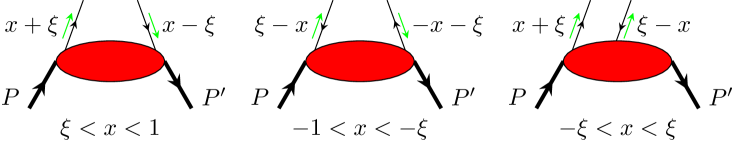
Figure 9: Parton interpretation of the GPDs in different kinematic regions.

The quark GPDs defined above have a number of remarkable properties, see, e.g., Ji (1998, 2004); Diehl (2003); Belitsky and Radyushkin (2005) , which either hold or have similar counterparts for the quark quasi-GPDs to be defined below. Apart from their physical significance, these properties also serve as useful checks on calculations related to GPDs.

According to LaMET, the unpolarized quark GPDs defined above can be determined by calculating the following quasi-GPDs

$$\tilde{F} =\frac{1}{2{\bar{P}}^{0}}\int\frac{d\lambda}{2\pi}e^{iy\lambda}\langle P^{\prime}S^{\prime}|{O}_{\gamma^{0}}(z)|PS\rangle$$

$$=\frac{1}{2{\bar{P}}^{0}}\bar{u}(P^{\prime}S^{\prime})\bigg{\{}\tilde{H}\gamma^{0}+\tilde{E}\frac{i\sigma^{0\mu}\Delta_{\mu}}{2M}\bigg{\}}u(PS)\,,$$ (143)

where we have again suppressed the arguments $(y,\tilde{\xi},t,{\bar{P}}^{z},\mu)$ of $\tilde{F}$, $\tilde{H}$, and $\tilde{E}$. The operator ${O}_{\gamma^{0}}(z)=\bar{\psi}(\frac{z}{2})\gamma^{0}W(\frac{z}{2},-\frac{z}{2})\psi(-\frac{z}{2})$ is the same operator defining the unpolarized quark quasi-PDF, and $\lambda=z{\bar{P}}^{z}$. As in the quasi-PDF case, the momentum fraction $y$ extends from $-\infty$ to $\infty$. The skewness parameter for the quasi-GPD

$$\tilde{\xi}=-\frac{P^{\prime z}-P^{z}}{P^{\prime z}+P^{z}}=-\frac{\Delta^{z}}{2{\bar{P}}^{z}}=\xi+\mathcal{O}\left({M^{2}\over({\bar{P}}^{z})^{2}},{t\over({\bar{P}}^{z})^{2}}\right)$$ (144)

differs from the light-cone skewness $\xi$ by power suppressed corrections. Moreover, the constraint from $\vec{\Delta}_{\perp}^{2}\geq 0$ becomes Ji et al. (2015a)

$${\tilde{\xi}}\leq\frac{1}{2{\bar{P}}^{z}}\sqrt{\frac{-t\left[({\bar{P}}^{z})^{2}+M^{2}-t/4\right]}{M^{2}-t/4}},$$ (145)

which differs from the constraint in Eq. (142) by corrections of $\mathcal{O}(M^{2}/({\bar{P}}^{z})^{2},t/({\bar{P}}^{z})^{2})$. We can replace $\tilde{\xi}$ with $\xi$ and attribute the difference to generic power suppressed contributions.

The quasi-GPDs defined above can be renormalized by observing that their UV divergence depends only on the operators defining them, but not on the external states. Since ${O}_{\gamma^{0}}(z)$ is multiplicatively renormalized, we can choose the same renormalization factor as that for the quasi-PDF Stewart and Zhao (2018); Liu et al. (2020) to renormalize the quasi-GPD. After renormalization, the quasi-GPD can then be matched to the usual GPD through a factorization formula.

The factorization of quasi-GPDs was first proposed and verified at one-loop order in Ji et al. (2015a); Xiong and Zhang (2015), where a transverse momentum cutoff and a quark mass were used as the UV and IR regulator, respectively. Later on, a detailed derivation based on OPE was given in Liu et al. (2019a). In contrast with the OPE for the quasi-PDF, a crucial difference here is that the total derivative of operators can come into play, as it simply gives momentum transfer factors when sandwiched between non-forward external states, and therefore is non-vanishing. In other words, the local twist-two operators as those in Eq. (III.3) will mix under renormalization with operators with total derivatives. The RGE that governs the mixing reads Braun et al. (2003),

$$\mu^{2}{d\over d\mu^{2}}O^{{\mu}_{0}{\mu}_{1}\ldots{\mu}_{n}}(\mu)=\sum_{m=0}^{[n/2]}\Gamma_{nm}$$ (146)

$$\times\left[i\partial^{(\mu_{1}}\cdots i\partial^{\mu_{2m}}\bar{\psi}\gamma^{\mu_{0}}i\overleftrightarrow{D}^{\mu_{2m+1}}\cdots i\overleftrightarrow{D}^{\mu_{n})}\psi-{\rm trace}\right]\,,$$

where $\Gamma_{nm}$ is the anomalous dimension of the associated operators, $\overleftrightarrow{D}=(\overrightarrow{D}-\overleftarrow{D})/2$ with $\overrightarrow{D}(\overleftarrow{D})$ denoting the covariant derivative acting to the right (left). The above equation can be diagonalized by choosing an appropriate operator basis. Such an operator basis has been studied in the literature and known as the “renormalization group improved” conformal operators Braun et al. (2003); Mueller (1994b). In terms of the matrix elements of these operators, we have

$$\langle P^{\prime}|{O}_{\gamma^{0}}(z)|P\rangle=2P^{0}\sum_{n=0}^{\infty}C_{n}({\mu}^{2}z^{2}){\cal F}_{n}(-\lambda)\sum_{m=0}^{n}{\cal B}_{nm}(\mu)$$

$$\hskip 30.00005pt\times\xi^{n}\int_{-1}^{1}dx\ C_{m}^{3/2}\left({x\over\xi}\right)F(x,\xi,t,\mu)+\ldots\,,$$ (147)

where ${\cal F}_{n}(-\lambda)$ are partial wave polynomials whose explicit forms are known in the conformal OPE of current-current correlators for the hadronic light-cone DAs Braun and Müller (2008), ${\cal B}_{nm}$ can be found in Braun et al. (2003); Mueller (1994b), and $\ldots$ denotes the higher-twist contributions $\mathcal{O}\left({M^{2}/({\bar{P}}^{z})^{2}},{t/({\bar{P}}^{z})^{2}},z^{2}\Lambda_{\rm QCD}^{2}\right)$.

Fourier transforming the l.h.s of the above equation to momentum space and invert it order by order in $\alpha_{s}$, we then obtain the following EFT expansion of the unpolarized quark GPD,

$$F(x,\xi,t,\mu)$$ (148)

$$\hskip 5.0pt=\int_{-\infty}^{\infty}{dy\over|\xi|}\bar{C}\left({x\over\xi},{y\over\xi},{\mu\over\xi{\bar{P}}^{z}}\right){\tilde{F}}(y,\xi,t,{\bar{P}}^{z},\mu)+\ldots$$

$$\hskip 5.0pt=\int_{-\infty}^{\infty}{dy\over|y|}C\left({x\over y},{\xi\over y},{\mu\over y{\bar{P}}^{z}}\right){\tilde{F}}(y,\xi,t,{\bar{P}}^{z},\mu)+\ldots\,,$$

which has been organized following the same spirit as the factorization of PDFs in previous sections. Both forms have been used in the literature Ji et al. (2015a); Xiong and Zhang (2015); Liu et al. (2019a) with the matching coefficients being related by

$$C\left({x\over y},{\xi\over y},{\mu\over y{\bar{P}}^{z}}\right)=\left|{y\over\xi}\right|\bar{C}\left({x\over\xi},{y\over\xi},{\mu\over\xi{\bar{P}}^{z}}\right)\,,$$ (149)

and $\ldots$ denotes the higher-twist contributions which have the same power-counting as in Eq. (IV.1) except that $z^{2}$ is replaced by $1/(x{\bar{P}}^{z})^{2}$. For the helicity and transversity quark quasi-GPDs, the factorization formula has the same form as Eq. (148) Liu et al. (2019a).

The matching coefficient can be obtained by replacing the hadron states in Eqs. (IV.1) and (IV.1) with the quark states carrying momentum $p+\Delta/2$ and $p-\Delta/2$ with $p^{\mu}=(p^{0},0,0,p^{z})$, and calculating the quark matrix element in perturbation theory. The explicit expression for the $\mathcal{O}(\alpha_{s})$ matching coefficients can be found in Liu et al. (2019a). An important feature of the result is: The quasi-GPDs do not vanish in all $y$ range, but the collinear singularities only show up in DGLAP and ERBL regions at one-loop. They are exactly the same as those in light-cone GPDs, and thus cancel in the matching coefficient. Moreover, one can derive momentum RGEs for the quasi-GPDs, which are turned into RGE for the scale dependence of the GPDs by the matching procedure.

To conclude this subsection, let us make some remarks on the EFT formula for the quark GPD above. First, at zero skewness $\xi=0$, we have

$$F(x,0,t,\mu) =\!\!\int_{-\infty}^{\infty}\!{dy\over|y|}C\!\left({x\over y},0,{\mu\over y{P}^{z}}\right)\!{\tilde{F}}(y,0,t,P^{z},\mu)$$

$$\qquad+\ldots\,,$$ (150)

where the matching kernel $C(x/y,0,\mu/(yP^{z}))$ is exactly the same as the matching coefficient for the quasi-PDF Izubuchi et al. (2018), even when $t\neq 0$. This can be understood as follows: At zero skewness, both the longitudinal momentum transfer and the energy transfer vanish, the momentum transfer is purely transverse and thus is not affected by Lorentz boost along the longitudinal $z$ direction. As a result, no extra matching related to $t$ is required in the large $P^{z}$ limit, and the matching remains the same as in the quasi-PDF case. If we take the forward limit $\Delta\to 0$, then Eq. (IV.1) reduces exactly to the EFT expansion formula for the PDF Ji et al. (2015a); Izubuchi et al. (2018).

Second, in the limit $\xi\to 1$ and $t\to 0$, the quasi-GPD reduces to the quasi-DA that will be discussed in the next subsection, and the corresponding matching kernel also reduces to that for the quasi-DA.

IV.2 Hadronic Distribution Amplitudes

Within LaMET, the DAs of protons as well as other hadrons can also be extracted from lattice simulations of appropriately chosen quasi-DAs. In this subsection, we show how this can be done in practice. For illustration, we take the leading-twist pion DA as an example. The application to other hadrons Zhang et al. (2019c); Wang et al. (2019a) is analogous.

The leading-twist DA of the pion is the simplest and most extensively studied hadronic DA. It represents the probability amplitude of finding the valence $q\bar{q}$ Fock state in the pion with the quark carrying a fraction $x$ of the total pion momentum, and is defined as

$$\phi_{\pi}(x) ={\frac{1}{if_{\pi}}}\int\frac{d\lambda}{2\pi P^{+}}e^{-i(x-\frac{1}{2})\lambda}\langle 0|O_{\gamma^{+}\gamma_{5}}(\lambda n)|\pi(P)\rangle\,,$$ (151)

with normalization $\int_{0}^{1}dx\,\phi_{\pi}(x)=1$. Here $f_{\pi}$ denotes the decay constant, and $O_{\gamma^{+}\gamma_{5}}(\lambda n)$ has the same structure as that used in Eq. (IV.1) with $\gamma^{+}$ replaced by $\gamma^{+}\gamma_{5}$. The pion DA can be constrained from experimental measurements of, e.g., $\gamma\gamma*\rightarrow\pi^{0}$ from BaBar and Belle Aubert et al. (2009); Uehara et al. (2012), and then used as an input to test QCD in other measurements such as the pion form factor Efremov and Radyushkin (1980); Farrar and Jackson (1979). In the asymptotic limit, it is well known that the pion DA takes the form $6x(1-x)$ Efremov and Radyushkin (1980); Lepage and Brodsky (1979). However, how it behaves at lower scales remains under debate (see e.g. Chernyak and Zhitnitsky (1982)). Calculating the pion DA with controllable systematics in LaMET will be able to shed new lights on its shape and thus on our understanding of pion structure.

Following the same strategy as before, we can access the $x$-dependence of the pion DA by studying the following quasi-DA Ji et al. (2015a); Zhang et al. (2017)

$$\tilde{\phi}_{\pi}(y,P^{z}) ={\frac{1}{if_{\pi}}}\int\frac{d\lambda}{2\pi P^{z}}e^{i(y-\frac{1}{2})\lambda}\langle 0|{O}_{\gamma^{z}\gamma_{5}}(z)|\pi(P)\rangle\,,$$ (152)

The longitudinally and transversely polarized vector meson quasi-DAs can be defined analogously by replacing $\gamma^{z}\gamma_{5}$ in the above equation with $\gamma^{0}$, $\gamma^{z}\gamma_{\perp}$, respectively Liu et al. (2019b).

The quark bilinear operators defining quasi-DAs follow the same renormalization pattern as those defining the quasi-PDFs or quasi-GPDs. In the literature, the Wilson-line mass-subtraction scheme was used in the first LaMET calculations of the meson DAs Zhang et al. (2017, 2019c), and the RI/MOM scheme has been adopted in more recent works Zhang et al. (2020b).

The LaMET expression for DAs takes the following form in the ${\overline{\rm MS}}$ scheme Ji et al. (2015a); Liu et al. (2019b)

$$\phi_{\pi}(x,\mu) =\int_{-\infty}^{\infty}dy\,C_{\pi}\left(x,y,P^{z}/\mu\right)\tilde{\phi}_{\pi}(y,P^{z},\mu)+\ldots\,.$$ (153)

The matching coefficient for the quasi-DAs can be obtained by replacing the meson state $|\pi(P)\rangle$ in Eqs. (151) and (152) with the lowest Fock state $|q(yP)\bar{q}((1-y)P)\rangle$ and calculating the quark matrix elements, where $yP$ and $(1-y)P$ are the momenta of the quark $q$ and anti-quark $\bar{q}$, respectively. Its one-loop results have been calculated in both ${\overline{\rm MS}}$ and RI/MOM schemes Liu et al. (2019b), which agrees with matching coefficient for the quasi-GPDs Ji et al. (2015a); Xiong and Zhang (2015); Liu et al. (2019a) in Eq. (148) with the replacement of $\xi\to 1/(2y-1)$, $x/\xi\to 2x-1$, and the external momentum $p^{z}$ to $p^{z}/2$.

Apart from the LaMET approach in momentum space, the shape of the pion DA has also been studied using equal-time current-current correlation in coordinate space approach Bali et al. (2018b, a),

$$\langle 0|T\Big{\{}J_{\mu}\Big{(}\frac{z}{2}\Big{)}J_{\nu}\Big{(}-\frac{z}{2}\Big{)}\Big{\}}|\pi^{0}(P)\rangle$$

$$\hskip 30.00005pt=\frac{2i\,f_{\pi}}{3\pi^{2}z^{4}}\epsilon_{\mu\nu\alpha\beta}P^{\alpha}z^{\beta}\Phi_{\pi}(\lambda,z^{2})\,,$$ (154)

where $\Phi_{\pi}(\lambda,z^{2})$ can be factorized as

$$\Phi_{\pi}(\lambda,z^{2}) =C_{2}(\lambda,z^{2}\mu^{2},x)\otimes\phi_{\pi}(x,\mu)+\cdots\,.$$ (155)

Here the matching coefficient $C_{2}$ depends on the choice of the currents. Its explicit expression can be found in Bali et al. (2018a). The above factorization is controlled by ${\mathcal{O}}(z^{2}\Lambda_{\rm QCD}^{2})$, with power corrections denoted by “$\cdots$”. In Bali et al. (2018a), a combined analysis of several current-current correlations has been performed where twist-four contributions were also included using the model estimate in Braun and Filyanov (1990); Ball et al. (2006). The leading-twist pion DA was then extracted from a global fit to the data, and the second moment of the pion DA has been fitted with controlled precision, both of which favor a considerably broader shape than the asymptotic DA at a scale of $2$ GeV. A large pion momentum is required to access information at large $\lambda$ so that we can extract wider range of $x$ or higher moments of the pion DA Bali et al. (2018b).

IV.3 Higher-Twist Distributions

Higher-twist distributions are quantities of great interest because they describe the coherent quark-gluon correlations in the proton. In contrast with the leading-twist distributions, our understanding of the higher-twist ones is rather poor. On one hand, they often depend on more than one parton momentum fractions; on the other hand, there is no physical intuition about what they may look like, in particular, about how they behave asymptotically at small and large $x$ Braun et al. (2011). There have been studies on the higher-twist distributions in the context of their connection to the DIS structure function, the transverse single-spin asymmetries in various hadron productions, GPDs related to quark and gluon OAM, parton DAs, etc. LaMET will be able to shed new lights by providing a possibility to access them from the lattice.

Higher-twist contributions also appear in LaMET expansion, where the suppression is provided by powers of the hadron momentum squared. In all factorizations presented in previous sections, only the leading-twist terms that capture the logarithmic dependence on hadron momentum are taken into account. The higher-twist contributions have been assumed to be small. If the hadron momentum is not sufficiently large compared and/or one is close to the endpoint region ($x\to 0$ and $x\to 1$), the higher-twist contributions can become non-negligible, whose structure and impact require understanding.

IV.3.1 Higher-twist collinear-parton observables

Beyond leading-twist, there exist three simplest twist-three quark distributions $e(x)$, $g_{T}(x)$ and $h_{L}(x)$ related to the unpolarized, transversely and longitudinally polarized proton Jaffe and Ji (1992),

$$e(x) =\frac{1}{2M}\int\frac{d\lambda}{2\pi}e^{ix\lambda}$$ (156)

$$\quad\times\langle PS|\psi^{\dagger}_{+}(0)\gamma_{0}\psi_{-}(\lambda n)|PS\rangle+{\rm h.c.}\,,$$

$$g_{T}(x) =\frac{1}{2M}\int\frac{d\lambda}{2\pi}e^{ix\lambda}$$ (157)

$$\quad\times\langle PS_{\perp}|\psi^{\dagger}_{+}(0)\gamma_{0}\gamma_{\perp}\gamma_{5}\psi_{-}(\lambda n)|PS_{\perp}\rangle+{\rm h.c.}\,,$$

$$h_{L}(x) =\frac{1}{2M}\int\frac{d\lambda}{2\pi}e^{ix\lambda}$$ (158)

$$\quad\times\langle PS_{z}|\psi^{\dagger}_{+}(0)\gamma_{0}\gamma_{5}\psi_{-}(\lambda n)|PS_{z}\rangle+{\rm h.c.}\,,$$

where we have again employed the decomposition of quark fields $\psi=\psi_{+}+\psi_{-}$ in Sec. I.1 and the light-cone gauge $A^{+}=0$, and “h.c.” stands for Hermitian conjugate.

The twist-three distributions can contribute as leading effects in certain experimental observables. For example, $g_{T}(x)$ and $h_{L}(x)$ can be measured as the leading effects in the longitudinal-transverse spin asymmetry in polarized Drell-Yan process.

Since $\psi_{-}$ is a non-dynamical component depending on $\psi_{+}$, all the above distributions can be shown to be related to more complicated quark-gluon correlation functions Ji and Chou (1990); Balitsky et al. (1996). A complete set of such correlation functions has been given in Qiu and Sterman (1991); Ji (1992); Ji and Osborne (2001); Kang and Qiu (2009), where the quark-gluon correlations in a transversely-polarized proton take the following form

$$T_{q}(x_{1},x_{2})=\frac{1}{(P^{+})^{2}}\int\frac{d\lambda d\zeta}{(2\pi)^{2}}e^{i\lambda x_{1}+i\zeta(x_{2}-x_{1})}$$ (159)

$$\hskip 20.00003pt\times\langle PS_{\perp}|\bar{\psi}(0)\gamma^{+}\epsilon^{+-S_{\perp}i}gF^{+i}(\zeta n)\psi(\lambda n)|PS_{\perp}\rangle,$$

$$T_{\Delta q}(x_{1},x_{2})=\frac{1}{(P^{+})^{2}}\int\frac{d\lambda d\zeta}{(2\pi)^{2}}e^{i\lambda x_{1}+i\zeta(x_{2}-x_{1})}$$ (160)

$$\hskip 20.00003pt\times\langle PS_{\perp}|\bar{\psi}(0)i\gamma^{+}\gamma_{5}S^{i}_{\perp}gF^{+i}(\zeta n)\psi(\lambda n)|PS_{\perp}\rangle\,.$$

There are also ones in an unpolarized and longitudinally-polarized proton. Generalizing to off-forward kinematics, the resulting twist-three GPDs are also related to quark and gluon OAM contribution to the proton spin Hatta and Yoshida (2012); Ji et al. (2013a).

One can also define twist-four distributions in a similar way as in Eq. (IV.3.1) by using $\psi_{-}$ for both quark fields. More general twist-four distributions will involve three light-cone variables, which will contribute to, e.g., $1/Q^{2}$ term in DIS Jaffe and Soldate (1982); Ellis et al. (1983); Jaffe and Ji (1992); Ji (1993).

In principle, all the above higher-twist distributions, as well as others that have not been listed here, can be computed using the LaMET approach by choosing appropriate quasi-LF correlations. For example, the first exploratory lattice calculation of $g_{T}(x)$ has been done in Bhattacharya et al. (2020a), which will be discussed in Sec. VI.3. However, extra complications are expected due to their complex structure. For instance, the lightcone zero modes that do not enter in dealing with leading-twist distributions come into play here. Recently, one of the authors has shown how to study the properties of these zero modes from lattice simulations in LaMET Ji (2020). In addition, the higher-twist distributions will have a more complex mixing pattern Ji and Chou (1990); Balitsky et al. (1996). Thus, their matching from the corresponding quasi distributions must take into account such mixings, making them more challenging than calculating the twist-two PDFs. One-loop studies of the matching for twist-three disributions have been carried out in Bhattacharya et al. (2020b, c).

IV.3.2 Higher-twist contributions to quasi-PDFs

Let us turn to the power suppressed higher-twist contributions appearing in the extraction of leading-twist quark PDFs using LaMET. Such contributions have two distinct origins. To understand them, let us recall the OPE for the quasi-LF correlation in Eq. (III.3). For simplicity, we ignore the renormalization here. Recovering the leading-twist quark PDF requires removing the contributions of both trace terms in that equation. The trace terms on the r.h.s. of Eq. (III.3), which lead to contributions suppressed by powers of $M^{2}/(P^{z})^{2}$, are known as kinematic power contributions or target mass corrections. In DIS, they can be accounted for by changing the scaling variable $x$ to the Nachtmann variable Nachtmann (1973). In the case of LaMET, it behaves slightly differently, as shown in the following. The second type of power corrections come from the trace terms in the operators on the r.h.s. of Eq. (III.3), and in general leads to contributions of $\mathcal{O}(\Lambda^{2}_{\rm{QCD}}/(P^{z})^{2})$ . These are genuine higher-twist contributions that involve multi-parton correlations, sometimes also known as dynamical higher-twist contributions. The target mass corrections have been computed to all orders in $M^{2}/(P^{z})^{2}$ for the quark quasi-PDFs in Chen et al. (2016); Radyushkin (2017c). The genuine higher-twist contributions have been investigated using two different approaches Chen et al. (2016); Braun et al. (2019).

According to Chen et al. (2016), the $M^{2}/(P^{z})^{2}$ corrections can be obtained from the ratio

$$K_{m} \equiv\frac{n_{(\mu_{1}}\cdots n_{\mu_{m})}P^{\mu_{1}}\cdots P^{\mu_{m}}}{n_{\mu_{1}}\cdots n_{\mu_{m}}P^{\mu_{1}}\cdots P^{\mu_{m}}}=\sum_{i=0}^{i_{\text{max}}}C_{m-i}^{i}c^{i}\,,$$ (161)

where $i_{\text{max}}=(m-\text{Mod}[m,2])/2$, $C$ is the binomial function and $c=-n^{2}M^{2}/4\left(n\cdot P\right)^{2}=M^{2}/4(P^{z})^{2}$ with $n^{\mu}=(0,0,0,-1)$ and $n\cdot P=P^{z}$.

Plugged into the tree-level OPE formula in Eq. (III.3), the above factors can then be converted to the following relation between unpolarized PDF and quasi-PDF Chen et al. (2016)

$$q(x) =\sqrt{1+4c}\sum_{n=0}^{\infty}\frac{(4c)^{n}}{f_{+}^{2n+1}}\Big{[}(1+(-1)^{n})\tilde{q}\Big{(}\frac{f_{+}^{2n+1}x}{2(4c)^{n}}\Big{)}$$

$$\qquad+(1-(-1)^{n})\tilde{q}\Big{(}\frac{-f_{+}^{2n+1}x}{2(4c)^{n}}\Big{)}\Big{]},$$ (162)

where $f_{+}=\sqrt{1+4c}+1$. It is worth noting that quark number conservation is preserved in the above result. The target mass corrections for the longitudinally and transversely polarized quasi-PDFs can be derived analogously.

The trace part on the r.h.s. of Eq. (III.3) is a genuine higher-twist effect. One may try to construct a non-local form of the higher-twist operators from OPE. The leading trace term, which is a twist-four effect, has been studied in Chen et al. (2016) (see also Balitsky and Braun (1989)) and shown to give rise to a twist-four PDF

$${q}_{\text{4}}(x,P^{z})=\int_{-\infty}^{\infty}\!\frac{d\lambda}{8\pi P^{z}}\,\Gamma_{0}\left(-ix\lambda\right)\left\langle P\left|O_{\text{tr}}(z)\right|P\right\rangle,$$ (163)

with

$$O_{\text{tr}}(z)=\int_{0}^{z}\!dz_{1}\,\bar{\psi}(0)\Big{[}\Gamma^{\nu}W\left(0,z_{1}\right)D_{\nu}W\left(z_{1},z\right)$$ (164)

$$+\int_{0}^{z_{1}}\!\!\!dz_{2}\,n\cdot\Gamma\,W\left(0,z_{2}\right)D^{\nu}W\left(z_{2},z_{1}\right)D_{\nu}W\left(z_{1},z\right)\Big{]}\psi(zn)\,,$$

where one has $\Gamma^{\mu}=\gamma^{\mu},\gamma^{\mu}\gamma^{5},\gamma^{\perp}\gamma^{\mu}\gamma^{5}$ for the unpolarized, helicity and transversity PDFs, respectively. $\Gamma_{0}$ is the incomplete Gamma function

$$\Gamma_{0}\left(-ix\right)=\int_{0}^{1}\frac{dt}{t}e^{ix/t}\,.$$ (165)

The above twist-four contribution needs to be removed from the quasi-PDF to recover the leading-twist PDF. It also provides a possibility for practical computations on the lattice. However, as a multi-parton correlation involving more gauge links and covariant derivatives, its lattice computation is rather challenging and has not been carried out in any existing work yet.

Another approach that has been used to estimate power corrections related to quark quasi-PDFs is the renormalon model (see Beneke (1999) for a comprehensive review). It is based on the observation that the perturbative expansion of the matching coefficient for the quasi-PDF diverges factorially with the loop order, implying that it is only well defined up to a power accuracy. This is known as the renormalon ambiguity, which must be cancelled by terms in the higher-twist contributions.

In Braun et al. (2019), it was shown that the cancellation of renormalon ambiguity requires that the leading higher-twist or twist-four contribution takes the following form

$${q}_{4}(y,P^{z},\mu)=\mu^{2}\int_{-1}^{1}\!\frac{dx}{|x|}D\Big{(}\frac{y}{x}\Big{)}q(x,\mu)+q^{\prime}_{4}(y,P^{z},\mu)\,,$$ (166)

where the first term on the r.h.s. cancels the renormalon ambiguity from the leading-twist matching coefficient, and $q^{\prime}_{4}$ depends on $\mu$ at most logarithmically. Since the first term is to merely cancel similar contributions in the matching coefficient, it does not contribute to any physical observable. The renormalon model of power corrections Beneke and Braun (1995); Dokshitzer et al. (1996); Dasgupta and Webber (1996, 1997); Beneke et al. (1997); Braun et al. (2004) is based on the assumption that, by replacing $\mu$ with a suitable nonperturbative scale, this contribution reflects the order and the functional form of actual power-suppressed contributions. This was known as “ultraviolet dominance” in Braun (1995); Beneke (1999); Beneke and Braun (2000). Under this assumption, we obtain the following estimate,

$${q}_{4}(y,P^{z},\mu)=\kappa\Lambda_{\rm QCD}^{2}\int_{-1}^{1}\!\frac{dx}{|x|}D\Big{(}\frac{y}{x}\Big{)}\,q(x,\mu)\,,$$ (167)

where $\kappa$ is a dimensionless coefficient of $\mathcal{O}(1)$ that cannot be fixed within theory and remains a free parameter.

A detailed analysis Braun et al. (2019) showed that for the quasi-PDF we have

$${q}_{4}(y,P^{z})=\frac{\kappa\Lambda_{\rm QCD}^{2}}{y^{2}(1-y)(P^{z})^{2}}$$ (168)

$$\times(1-y)\!\Big{[}\!\!\int_{|y|}^{1}\!\!\frac{dx}{x}\Big{[}\frac{x^{2}}{(1-x)_{+}}\!-\!2x^{2}\Big{]}q\Big{(}\frac{y}{x}\Big{)}\!+\!2q(y)\!-\!|y|q^{\prime}(y)\Big{]}\,,$$

where the first term in the integral was reproduced in a recent analysis of the renormalon effects in the quasi-PDF Liu and Chen (2020). As one can see, the second row vanishes as $q(y)$ when $y\to 1$ if $\lim_{y\to 1}q(y)\sim(1-y)^{a}$ with $a>0$. This gives an estimate of the twist-four contribution on the r.h.s. of Eq. (II.3), which implies that the higher-twist contributions are enhanced as $1/y^{2}$ and $1/(1-y)$ for $y\sim 0$ and $y\sim 1$, respectively. Similar analysis can also be done for the pseudo-PDF. The above result can be used as a way to model the twist-four contribution with $\kappa$ as the only parameter.

IV.4 Orbital Angular Momemntum of Partons in the Proton

Over the past three decades, much experimental and theoretical work has been done on the origin and structure of proton spin, which has been covered in depth in the review articles  Filippone and Ji (2001); Bass (2005); Aidala et al. (2013); Leader and Lorcé (2014); Ji (2017); Deur et al. (2019); Ji et al. (2020c).

In addition to the spin-dependent PDFs and TMDs, the GCPOs—in particular the GPDs—also play an important role in understanding the spin structure of the proton. Since GPDs describe the correlation between the transverse position and longitudinal momentum of quarks and gluons inside the proton, they offer a unique channel to study the orbital angular momentum (OAM) from experiments.

There are two widely known definitions of OAM in literature. One is the kinetic OAM in the gauge-invariant and frame-independent sum rule for the proton spin Ji (1997b, a), which is related to the first moment of twist-two GPDs and can be calculated from the form factors of the symmetric QCD energy-momentum tensor. A review of the lattice calculations of kinetic OAM can be found in Ji et al. (2020c). The other definition, which has a clear partonic interpretation in comparison to the kinetic OAM, is the canonical OAM in the naive partonic sum rule Jaffe and Manohar (1990) based on the free-field form of the QCD angular momentum,

$$\vec{J} =\int d^{3}\xi\ \psi^{\dagger}\frac{\vec{\Sigma}}{2}\psi+\int d^{3}\xi\ \psi^{\dagger}\left[\vec{\xi}\times(-i\vec{\nabla})\right]\psi$$

$$\ \ \ \ \ +\int d^{3}\xi\ \vec{E}\times\vec{A}+\int d^{3}\xi\ E^{i}\ \left(\vec{\xi}\times\vec{\nabla}\right)A^{i}\ ,$$ (169)

where $i$ is the spatial Lorentz index. Except for the first one, the other three operators are gauge dependent, and their matrix elements are generally frame dependent. In high-energy scattering, there is one frame and gauge that are special: the IMF and light-front gauge, $A^{+}=0$. Therefore, the naive partonic sum rule for proton spin can be expressed as Jaffe and Manohar (1990)

$$\frac{1}{2}=\frac{1}{2}\Delta\Sigma(\mu)+l^{z}_{q}(\mu)+\Delta G(\mu)+l^{z}_{g}(\mu)\,,$$ (170)

where $l^{z}_{q}(\mu)$ and $l^{z}_{g}(\mu)$ are the canonical OAM of the quark and gluon partons, respectively. Both $l_{q}^{z}$ and $l_{g}^{z}$ can be related to twist-three GPDs Hatta (2012); Ji et al. (2013a); Hatta and Yoshida (2012), which can be accessed through spin-asymmetries in hard exclusive processes Ji et al. (2017a); Hatta et al. (2017); Bhattacharya et al. (2017, 2018) (see the recent review Ji et al. (2020c)).

To fully understand the partonic spin structure of the proton, one also needs to determine the quark and gluon canonical OAM, $l^{z}_{q}$ and $l^{z}_{g}$. LaMET allows extraction of $l_{q}^{z}$ and $l_{g}^{z}$ from lattice calculation in the same way as the gluon helicity that was reviewed in Sec. III.5.

The quasi-partonic OAM operators can be chosen as the free-field operators fixed in gauges that belong to the universality class Hatta et al. (2014). Their matrix elements $\tilde{l}^{z}_{q}$ and $\tilde{l}^{z}_{g}$ can be calculated from the off-forward matrix elements of the relevant energy-momentum tensors Zhao et al. (2016), for example,

$$\tilde{l}^{z}_{q}(2S^{z}) =\lim_{\Delta\to 0}\epsilon^{ij}{\partial\over\partial i\Delta^{i}}\langle P^{\prime}S|\psi^{\dagger}(0)i\partial^{j}\psi(0)|PS\rangle\Big{|}_{\vec{\nabla}\cdot\vec{A}=0}\,.$$ (171)

where the kinematics is the same as Eq. (140).

Along with $\Delta G$, $\tilde{l}^{z}_{q}$ and $\tilde{l}^{z}_{g}$ can be matched to the partonic quantities defined in the Jaffe-Manohar sum rule through the factorization formulas,

$$\tilde{l}^{z}_{q}(P^{z},\mu) =P_{qq}l^{z}_{q}(\mu)+P_{gq}l^{z}_{g}(\mu)$$

$$\qquad+p_{qq}\Delta\Sigma(\mu)+p_{gq}\Delta G(\mu)+...\,,$$ (172)

$$\tilde{l}^{z}_{g}(P^{z},\mu) =P_{qg}l^{z}_{q}(\mu)+P_{gg}l^{z}_{g}(\mu)$$

$$\qquad+p_{qg}\Delta\Sigma(\mu)+p_{gg}\Delta G(\mu)+...\,,$$ (173)

where $\cdots$ are power corrections suppressed by the momentum $P^{z}$, and the one-loop matching coefficients in front of each term on the r.h.s. have been calculated in the Coulomb gauge Ji et al. (2015c). Since the quasi-partonic operators are gauge-variant and need to be fixed in a particular gauge, they can mix with new operators that are not allowed by Lorentz or gauge symmetries. For example, the gauge-dependent potential angular momentum $\psi^{\dagger}(\vec{r}\times\vec{A})\psi$ comes into play Wakamatsu (2014); Ji et al. (2016). Such mixings must be taken into account in lattice renormalization to have a controlled calculation of the canonical OAM.

Apart from the above approach, it has also been proposed to calculate the ratio of $l_{q}^{z}$ and the valence quark number from the derivatives of off-forward matrix elements of staple-shaped quark Wilson line operators Engelhardt (2017), whose definition can be found in Eq. (205) below. The first lattice calculations with this approach have been carried out in Engelhardt (2017); Engelhardt et al. (2018), which shows different size of effects between the kinetic and canonical OAM. For systematic improvement in this calculation, one should include the matching of such matrix elements to the physical $l_{q}^{z}$ in the limit when the transverse separation of the quark fields approaches zero.

For the transverse polarization, it is natural to define a twist-two partonic transverse angular momentum density of quarks Hoodbhoy et al. (1999b); Ji et al. (2012); Ji and Yuan (2020); Ji et al. (2020c),

$$J^{q}_{\perp}(x)=x\left[q(x)+E_{q}(x)\right]/2,$$ (174)

and similarly for the gluons, where $q(x)$ is the unpolarized quark/antiquark distributions, and $E_{q,g}(x)$ is the GPDs defined earlier in this section. Thus to get a simple partonic picture of the proton transverse spin from the first principles, it is important to calculate the GPD $E(x)$ using LaMET.

V Transverse-Momentum Dependent PDFs

The transverse-momentum-dependent (TMD) parton distribution functions (TMDPDFs) are a natural generalization of the collinear PDFs to include both longitudinal and transverse momentum of partons. They are in principle probability distributions $f_{i}(x,\vec{k}_{\perp},\sigma)$ of finding a parton of given species $i$, longitudinal and transverse momentum $(xP^{+},\vec{k}_{\perp})$, and polarization $\sigma$ inside the hadron state. TMDPDFs are playing an increasingly important role in understanding the partonic structure of hadrons and high-energy scattering.

The TMD parton densities were firstly introduced by Collins and Soper in 1980s Collins and Soper (1981, 1982a); Collins et al. (1983, 1985b, 1985a); Bodwin (1985) to understand the Drell-Yan (DY) and $e^{+}e^{-}$ annihilation process, and generalized in Ji et al. (2005, 2004) to semi-inclusive deep-inelastic scattering(SIDIS) process. The TMD factorization has been reanalyzed in the framework of SCET in which modes are made manifest by effective fields  Bauer et al. (2001, 2002); Manohar and Stewart (2007); Becher and Neubert (2011); Echevarria et al. (2012); Echevarría et al. (2013); Chiu et al. (2012). Various TMD factorization formalisms finally converged to the standard one where a scheme-independent TMDPDF can be defined Echevarría et al. (2013); Collins and Rogers (2013, 2017).

The TMD parton densities are important in understanding the experimental processes where the transverse momenta of final state particles are measured. For example, in DY pair and $W,Z$ production it is known that the differential cross section $d\sigma/dQ_{T}^{2}$ normally peaks at relatively small transverse momentum. For $Q\sim 10$ GeV, the peak is typically located at $Q_{\perp}\sim 1$ GeV where nonperturbative effects are important Collins et al. (1985b). A good knowledge of TMD parton densities is therefore crucial for the determination of the cross sections and precision test of perturbative QCD predictions.

Besides their importance in understanding the high-energy experimental data, the TMD parton densities are also important by themselves for their crucial role in describing hadron structures. With them, one can simultaneously study the fast-moving collinear physics through the longitudinal $x$-dependencies, and the nonperturbative effect from the transverse $\vec{k}_{\perp}$-dependencies. Moreover, the TMDPDFs are sensitive to effects such as soft radiations. Therefore, the physics in the presence of transverse degrees of freedom is rather rich. This is particularly true in studies of spin-dependent phenomena where one can define various TMDPDFs through Lorentz decompositions (see Sec. V.B). One example is the Sivers function for a transversely polarized proton, $\epsilon_{ij}k^{i}_{\perp}S^{i}_{\perp}f^{\perp}_{1T}(x,k_{\perp})$, which is naive-time-reversal odd and is predicted to change sign between the DY and SIDIS processes Collins (2011a). Similar properties also exist in the Boer-Mulders function Boer and Mulders (1998) concerning a transversely-polarized parton distribution in an unpolarized hadron. These two functions are related to the single transverse spin asymmetry. If we generalize the TMDPDFs to include the impact parameter dependence, we can further define the Wigner function, the parton orbital angular momentum distributions, etc Belitsky et al. (2004); Lorce et al. (2012). Therefore, the TMDPDFs allow for a more complete and refined 3D description (or tomography) of the hadron structure Burkardt (2000); Boer et al. (2011). The 3D tomography of the proton is a major physical goal of the EIC program. The TMDPDFs are also important in understanding small-$x$ physics Kuraev et al. (1977); Balitsky and Lipatov (1978); Balitsky (1996); Kovchegov (1999); Kovchegov and Levin (2012).

Our current knowledge on TMDPDFs mainly comes from fitting to the experimental data Landry et al. (2001); Konychev and Nadolsky (2006); Sun et al. (2018); Echevarria et al. (2014); Kang et al. (2016); Bacchetta et al. (2017); Scimemi and Vladimirov (2018a); Bertone et al. (2019); Scimemi and Vladimirov (2019); Bacchetta et al. (2019). This is, however, rather primitive due to the paucity of data. Although the future EIC will make up the gap and produce more data for TMD measurements, it is still important to develop first-principle methods for the determination of nonperturbative TMDPDFs, which can serve as a test or provide useful inputs to constrain the global fits. LaMET provides a systematic way to extract TMDPDFs from the lattice calculations. Early studies Ji et al. (2015b, 2019a); Ebert et al. (2019a, b) have tried to construct a quasi-TMDPDF on the lattice, but its relation to the physical TMDPDF is expected to be nonperturbative due to complications in the soft function Ebert et al. (2019b). The recent works in Ji et al. (2020a, 2019b) provide a formulation to calculate the soft function so that a perturbative matching formula can be established between the quasi- and physical TMDPDFs, allowing for a complete determination of the latter from lattice QCD. In this section we review the application of LaMET to the nonperturbative TMDPDFs. The investigation is still in its early stage and a lot remains to be explored, particularly in lattice calculations and matching.

In the first subsection we introduce the TMDPDFs and discuss the associated rapidity divergences. In the following subsections, we define the quasi-TMDPDFs or TMD momentum distributions in a proton of finite momentum, and study their momentum RGEs and UV renormalization properties. In the process, we introduce the off-light-cone soft functions. We then present the factorization of the quasi-TMDPDFs into the light-cone TMDPDFs and the off-light-cone soft function, where various one-loop results and the relevant RGEs are also given. The properties of the off-light-cone soft function are discussed in the last subsection, where it is shown to be related to the form factor of a pair of charged color sources, which paves the way for its calculation on a Euclidean lattice.

V.1 Introduction to TMDPDFs and Rapidity Divergence

As explained in Sec. II, we can define various TMDPDFs by choosing different gauge-links between the quark or gluon bilinears. The one relevant to high-energy phenomena is defined with light-like Wilson lines. The links represent the propagation of high-energy color-charged particles, and are crucial in forming gauge-invariant nonlocal operators Belitsky et al. (2003). As argued in previous sections, such operators are the result of an EFT description (more explicitly so in SCET) arising from taking the infinite-momentum limit of the proton. Thus, it is natural to expect that they require additional regularization and renormalization.

Let us take the non-singlet quark unpolarized TMDPDF as an example. Without the field theoretic subtleties, the distribution is

$$f(x,\vec{k}_{\perp})=\frac{1}{2P^{+}}\int\frac{d\lambda}{2\pi}\frac{d^{2}\vec{b}_{\perp}}{(2\pi)^{2}}e^{-i\lambda x+i\vec{k}_{\perp}\cdot\vec{b}_{\perp}}$$ (175)

$$\times\langle P|\bar{\psi}(\lambda n/2+\vec{b}_{\perp})\gamma^{+}{\cal W}_{n}(\lambda n/2+\vec{b}_{\perp})\psi(-\lambda n/2)|P\rangle\ ,$$

where ${\cal W}_{n}(\lambda n+\vec{b}_{\perp})$ is the staple-shaped gauge-link of the form

$${\cal W}_{n}(\xi)=W^{\dagger}_{n}(\xi)W_{\perp}W_{n}(-\xi\cdot pn)\ ,$$ (176)

$$W_{n}(\xi)={\cal P}\exp\left[-ig\int_{0}^{-\infty}d\lambda n\cdot A(\xi+\lambda n)\right]\ ,$$ (177)

along the light-cone direction $n^{\mu}$, as shown in Fig. 10.The $W_{\perp}$ is a transverse gauge-link at light-cone infinity to maintain gauge-invariance.. If one uses LFQ and ignores the transverse gauge-link, the above distribution is just $\langle P|b^{\dagger}(x,\vec{k}_{\perp})b(x,\vec{k}_{\perp})|P\rangle$ for $x>0$, as expected.

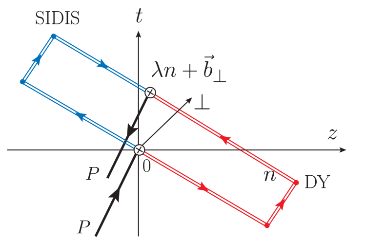
Figure 10: The space-time picture of TMDPDF for DY and SIDIS process. The circled crosses denote the quark-link vertices. Notice that the vertices are placed at $\lambda n+\vec{b}_{\perp}$ and $0$ which gives the same result as the symmetric choice in Eq. (175).

However, there are a number of qualifications in the above definition. First, the light-like gauge-links ${\cal W}_{n}$ are chosen to be past-pointing in accordance with the DY kinematics, but for SIDIS they should be chosen as future-pointing, as shown in Fig. 10. For unpolarized TMDPDFs there is no distinction between the two choices, but for spin-dependent TMDPDFs there are physical consequences associated with the direction of gauge-links.

Second, there exists a new type of divergence associated with the infinitely-long light-like gauge-links. These divergences are due to radiation of gluons collinear to the light-like gauge-link and cannot be regularized by the standard UV regulators. An example is the following integral in dimensional regularization (DR) Ebert et al. (2019b),

$$I=\int dk^{+}dk^{-}\frac{f(k^{+}k^{-})}{(k^{+}k^{-})^{1+\epsilon}}=\frac{1}{2}\int\frac{dy}{y}\int dm^{2}\frac{f(m^{2})}{m^{2+2\epsilon}}\,,$$ (178)

where $m^{2}=k^{+}k^{-}$ and $y=k^{+}/k^{-}$ is the rapidity-related variable. The divergences in $y$ arise from large and small $y$ where the integral is unregulated. The contribution from $k^{+}=0$ is called the light-zero mode in LFQ, where it is also called light-cone divergence which causes considerable problems.

To regulate the light-cone or rapidity divergences, a number of methods have been introduced in the literature (for a review see Ebert et al. (2019b)). They can be put into two classes: on-light-cone regulators and off-light-cone regulators. In the former case, the gauge-links are kept along the light-cone direction $n^{\mu}$ after regularization. For example, the so-called $\delta$ regulator Echevarria et al. (2016a, b) regularizes the gauge-link as:

$$W_{n}(\xi)\rightarrow W_{n}(\xi)|_{\delta^{-}}$$

$$={\cal P}{\rm exp}\left[-ig\int_{0}^{-\infty}d\lambda A^{+}(\xi+\lambda n)e^{-\frac{\delta^{-}}{2p^{+}}|\lambda|}\right]\,,$$ (179)

and similarly for the conjugate direction. The $\delta$ regulator breaks gauge-invariance, but preserves the boost invariance $\delta^{\pm}\rightarrow e^{\pm Y}\delta^{\pm}$ where $Y$ is the rapidity of the Lorentz boost. Other on-light-cone regulators include the exponential regulator Li et al. (2016), $\eta$ regulator Chiu et al. (2012), analytical regulator Becher and Neubert (2011), etc. In the remainder of this section, we will use the $\delta$ regulator as a representative whenever we need an on-light-cone regulator.

The off-light-cone regulator was introduced in  Collins and Soper (1981); Ji et al. (2005, 2004); Collins (2011a), and also used in  Ji et al. (2005). This type of regulator chooses off-light-cone directions to avoid the rapidity divergence. One can choose, for instance, to deform the gauge-links into the space-like region:

$$n\rightarrow n_{Y}=n-e^{-2Y}\frac{p}{(p^{+})^{2}}\,.$$ (180)

Here $Y$ plays the role of a rapidity regulator, as when $Y\rightarrow\infty$, $n_{Y}\rightarrow n$. In certain cases one can also deform $n_{Y}$ into time-like region Collins and Metz (2004).

The on-light-cone regulators are consistent with the spirit of parton physics, and therefore are useful to define COM-momentum-independent parton densities. The off-light-cone regulators, on the other hand, follow a similar spirit as LaMET, and therefore can be exploited for practical lattice QCD calculations, as we shall see in the next subsection.

To avoid light-cone divergences, from now on we include the rapidity regulator in the definition of the light-cone TMDPDFs. Using the same label $f$ for the TMDPDFs in both momentum and coordinate spaces, we have

$$f(\lambda,b_{\perp},\mu,\delta^{-}/P^{+})$$ (181)

$$=\langle P|\bar{\psi}(\lambda n/2+\vec{b}_{\perp})\not{n}{\cal W}_{n}(\lambda n/2+\vec{b}_{\perp})|_{\delta^{-}}\psi(-\lambda n/2)|P\rangle\,,$$

where $\mu$ is the ${\overline{\rm MS}}$ scale for UV renormalization. Due to rotational invariance, the bare TMDPDF defined above is a function of $b_{\perp}=|\vec{b}_{\perp}|$, so we have omitted the vector arrow for $\vec{b}_{\perp}$ in $f$ and will do so throughout the discussion for the soft functions, quasi-TMDPDFs, etc. The subscript $\delta^{-}$ denotes that the staple-shaped gauge-link ${\cal W}$ is regulated by the $\delta$ regulator in the light-cone minus direction. $f$ diverges logarithmically as $\delta^{-}\rightarrow 0$, and the finite part also depends on the rapidity regulator. To define the physical TMDPDF, we need to remove all divergences and rapidity regularization scheme dependencies in $f$, in a way similar to removing UV divergences in physical quantities.

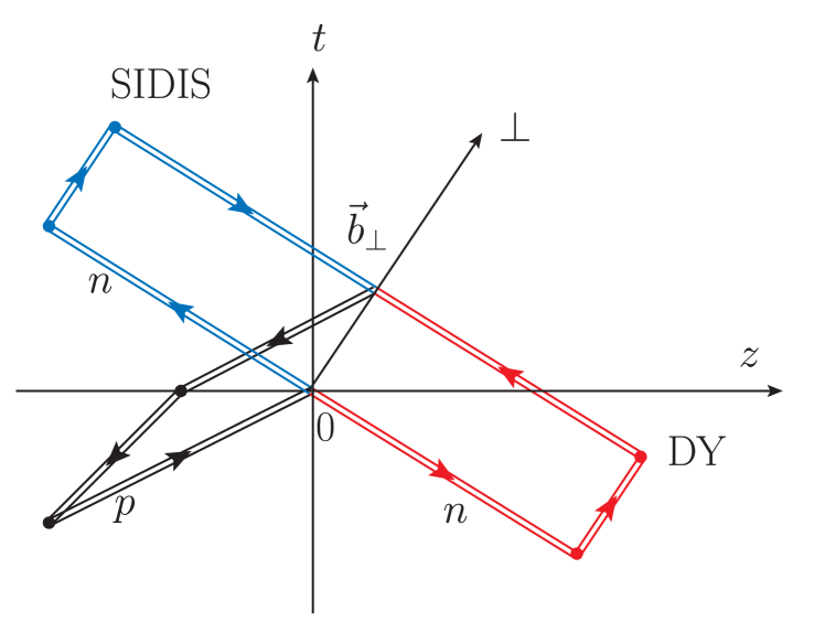
Figure 11: The soft function $S(b_{\perp},\mu,\delta^{+},\delta^{-})$ as space-time Wilson-loop arising in the factorization of DY and SIDIS process.

The rapidity divergence for TMDPDFs can be removed by the soft function, which also plays an important role in TMD factorization. Intuitively, the soft function represents a cross section for fast-moving charged particles emitting soft gluons into final states. It has rapidity divergence associated with the light-cone direction, which is ultimately related to the mass singularity. The TMD soft function corresponding to Drell-Yan process is defined Collins (2011b); Echevarria et al. (2016b) as

$$S(b_{\perp},\mu,\delta^{+},\delta^{-})$$

$$=\frac{{\rm Tr}\langle 0|{\cal\bar{T}}W_{p}(\vec{b}_{\perp})|_{\delta^{+}}W_{n}^{\dagger}(\vec{b}_{\perp})|_{\delta^{-}}{\cal T}W_{n}(0)|_{\delta^{-}}W^{\dagger}_{p}(0)|_{\delta^{+}}|0\rangle}{N_{c}}$$

$$=\frac{{\rm tr}\langle 0|{\cal W}_{n}(\vec{b}_{\perp})|_{\delta^{+}}{\cal W}^{\dagger}_{p}(\vec{b}_{\perp})|_{\delta^{-}}|0\rangle}{N_{c}}\,,$$ (182)

where ${\cal T}/\bar{\cal T}$ stands for time/anti-time ordering. The first equality defines the soft function in terms of cut-diagrams as an amplitude square. Since the soft function for DY process is independent of time ordering, one can also define it with a single time ordering or no time ordering, leading to the second equality. The staple-shaped gauge-link ${\cal W}_{n}$ is defined in Eq. (176), while the staple-shaped gauge-link ${\cal W}_{p}$ is defined similarly as:

$${\cal W}_{p}(\xi)=W^{\dagger}_{p}(\xi)W_{\perp}W_{p}(0)\ ,$$ (183)

$$W_{p}(\xi)={\cal P}{\rm exp}\left[-ig\int_{0}^{-\infty}d\lambda p\cdot A(\xi+p\lambda)\right]\ .$$ (184)

The soft function is shown in Fig. 11 as a Wilson loop in Minkowski space.

If the rapidity divergences are multiplicative, one can use $S$ as the rapidity renormalization factor for the TMDPDF defined in Eq. (175). In on-light-cone schemes such as the $\delta$ regularization, it has been argued in Vladimirov (2018) based on conformal transformation that the rapidity divergences are indeed multiplicative in position space. For each of the staple-shaped light-like gauge-links, the rapidity divergence is proportional to $\exp\left[-(1/2)K(b_{\perp},\mu)\ln\left(\mu^{2}/2(\delta^{\pm})^{2}\right)\right]$ where $K(b_{\perp},\mu)$ is the nonperturbative Collins-Soper evolution kernel Collins and Soper (1981). Thus at small $\delta^{\pm}$, we can write

$$S(b_{\perp},\mu,\delta^{+},\delta^{-})=e^{\ln\frac{\mu^{2}}{2\delta^{+}\delta^{-}}K(b_{\perp},\mu)+{\cal D}_{2}(b_{\perp},\mu)}\ \ ,$$ (185)

where ${\cal D}_{2}(b_{\perp},\mu)$ is a $b_{\perp}$-dependent but rapidity-independent function. Notice that our definitions of $\delta^{\pm}$ differ from those in Ref. Echevarria et al. (2016b) by a factor of $\sqrt{2}$ due to our normalization of light-cone vectors.

The soft-function in $\delta$ regularization satisfies the renormalization group equation

$$\mu^{2}\frac{d}{d\mu^{2}}\ln S(b_{\perp},\mu,\delta^{+},\delta^{-})$$

$$=-\Gamma_{\rm cusp}(\alpha_{s})\ln\frac{\mu^{2}}{2\delta^{+}\delta^{-}}+\gamma_{s}(\alpha_{s})\ ,$$ (186)

where $\Gamma_{\rm cusp}(\alpha_{s})$ is the light-like cusp anomalous dimension Polyakov (1980); Korchemsky and Radyushkin (1987) and the $\gamma_{s}(\alpha_{s})$ is the soft anomalous dimension Korchemskaya and Korchemsky (1992). The Collins-Soper kernel and the rapidity-independent part ${\cal D}_{2}$ satisfy the RGEs:

$$\mu^{2}\frac{d}{d\mu^{2}}K(b_{\perp},\mu)=-\Gamma_{\rm cusp}(\alpha_{s})\ ,$$ (187)

$$\mu^{2}\frac{d}{d\mu^{2}}{\cal D}_{2}(b_{\perp},\mu)=\gamma_{s}(\alpha_{s})-K(b_{\perp},\mu)\ .$$ (188)

At one-loop, the soft function $S(b_{\perp},\mu,\delta^{+},\delta^{-})$ is given by Echevarría et al. (2013) :

$$S(b_{\perp},\mu,\delta^{+},\delta^{-})$$

$$=1+\frac{\alpha_{s}C_{F}}{2\pi}\left(L_{b}^{2}-2L_{b}\ln\frac{\mu^{2}}{2\delta^{+}\delta^{-}}+\frac{\pi^{2}}{6}\right)\ ,$$ (189)

where $L_{b}=\ln\left(\mu^{2}b_{\perp}^{2}e^{2\gamma_{E}}/4\right)$. Therefore, we have at the leading order,

$$K(b_{\perp},\mu) =-\frac{\alpha_{s}C_{F}}{\pi}L_{b}\,,$$ (190)

$${\cal D}_{2}(b_{\perp},\mu) =\frac{\alpha_{s}C_{F}}{2\pi}\left(L_{b}^{2}+\frac{\pi^{2}}{6}\right)\ ,$$ (191)

and $\Gamma_{\rm cusp}=\alpha_{s}C_{F}/\pi+{\cal O}(\alpha_{s}^{2})$, $\gamma_{s}={\cal O}(\alpha_{s}^{2})$. It is worth pointing out that $K$ Li and Zhu (2017); Vladimirov (2017) and ${\cal D}_{2}$ Li and Zhu (2017) are known to 3-loop order in the exponential regularization scheme.

With the above soft function, we can take its square root to perform rapidity renormalization for the bare TMD correlator. The square root can be explained as follows: $S$ contains two staples, while $f$ contains one, thus the rapidity divergences as well as scheme dependencies in $S$ are twice as those in $f$. This leads to the following definition of the renormalized physical TMDPDF Echevarría et al. (2013); Collins and Rogers (2013):

$$f^{\rm TMD}(x,b_{\perp},\mu,\zeta)=\lim_{\delta^{-}\rightarrow 0}\frac{f(x,b_{\perp},\mu,\delta^{-}/P^{+})}{\sqrt{S(b_{\perp},\mu,\delta^{-}e^{2y_{n}},\delta^{-})}}\ ,$$ (192)

where the rapidity scale reads

$$\zeta=2(xP^{+})^{2}e^{2y_{n}}\ .$$ (193)

The rapidity dependence in the numerator of the right-hand side of Eq. (192) has the form $\exp[-\frac{1}{2}K(b_{\perp},\mu)\ln\frac{(\delta^{-})^{2}}{(xP^{+})^{2}}]$, while in the denominator it behaves as $\exp[\frac{1}{2}K(b_{\perp},\mu)\ln\frac{\mu^{2}}{2(\delta^{-})^{2}e^{2y_{n}}}]$. The $\delta^{-}$ dependence thus cancels out in the ratio, leaving a dependence on the rapidity scale as $\exp[-\frac{1}{2}K(b_{\perp},\mu)\ln\frac{\mu^{2}}{2(xP^{+})^{2}e^{2y_{n}}}]$, which is controlled by the so-called Collins-Soper evolution equation:

$$2\zeta\frac{d}{d\zeta}\ln f^{\rm TMD}(x,b_{\perp},\mu,\zeta)=K(b_{\perp},\mu)\ .$$ (194)

The $\zeta$-dependence comes from the initial-state quark radiation and is intrinsically nonperturbative for large $b_{\perp}$. $f^{\rm TMD}(x,b_{\perp},\mu,\zeta)$ is the standard object to be matched to in LaMET.

We should emphasize that although $f^{\rm TMD}$ is free from rapidity divergences, it does contain soft radiation from the charged particles in the initial state. This can be seen clearly by considering Feynman diagrams for the unsubtracted $f$ and applying soft approximation to gluons. “One-half” of the soft contribution in $f$ is subtracted to define the physical $f^{\rm TMD}$ due to the requirement of factorization of physical processes. The remaining soft radiation also has a natural rapidity cut-off associated with $\ln(xP^{+})$, reflected in the $\zeta$-dependence. What is remarkable, however, is that $f^{\rm TMD}$ is rapidity-regulator independent. Although a general proof to all orders in perturbation theory is beyond the scope of this review, it is due to factorization and exponentiation of the soft physics in $f$ and thus the scheme cancellation can be done systematically in the exponent. It worth mentioning that in old-fashioned or SCET-like approaches, one can define the “subtracted” TMDPDF or “beams functions” that contains only collinear physics. However, they are generically scheme dependent and must be combined with an extra soft functions in factorization theorems. At one-loop level, the scheme-independent one-loop TMDPDF for an external quark state reads,

$$f^{\rm TMD}(x,b_{\perp},\mu,\zeta)=\delta(1-x)$$

$$+\frac{\alpha_{s}C_{F}}{2\pi}F(x,\epsilon_{\tiny\mbox{IR}},b_{\perp},\mu)\theta(x)\theta(1-x)+\frac{\alpha_{s}C_{F}}{2\pi}\delta(1-x)$$

$$\times\left[-\frac{1}{2}L_{b}^{2}+\left(\frac{3}{2}-\ln\frac{\zeta}{\mu^{2}}\right)L_{b}+\frac{1}{2}-\frac{\pi^{2}}{12}\right]\ ,$$ (195)

where

$$F(x,\epsilon_{\tiny\mbox{IR}},b_{\perp},\mu)=\left[-\left(\frac{1}{\epsilon_{\tiny\mbox{IR}}}+L_{b}\right)\frac{1+x^{2}}{1-x}+1-x\right]_{+}\,.$$ (196)

Two-loop order results for the TMDPDFs can be found in Catani and Grazzini (2012); Catani et al. (2012); Gehrmann et al. (2014); Lübbert et al. (2016); Echevarria et al. (2016c); Luo et al. (2019) and three-loop order results can be found in Luo et al. (2020).

The physical TMDPDF also satisfies the RG equation,

$$\gamma_{\mu}(\mu,\zeta) =\mu^{2}\frac{d}{d\mu^{2}}\ln f^{\rm TMD}(x,b_{\perp},\mu,\zeta)$$

$$\equiv\frac{1}{2}\Gamma_{\rm cusp}(\alpha_{s})\ln\frac{\mu^{2}}{\zeta}-\gamma_{H}(\alpha_{s})\ ,$$ (197)

where $\gamma_{H}$ is called the hard anomalous dimension. At one-loop, the cusp and hard anomalous dimensions read

$$\Gamma_{\rm cusp}(\alpha_{s})=\frac{\alpha_{s}C_{F}}{\pi};~{}~{}~{}~{}~{}\gamma_{H}(\alpha_{s})=-\frac{3\alpha_{s}C_{F}}{4\pi}\ .$$ (198)

Recently the cusp anomalous dimension have been calculated to 4-loops Henn et al. (2019); von Manteuffel et al. (2020).

Combining the RGE and the rapidity evolution equation for the TMDPDF, one obtains the consistency condition :

$$\mu^{2}\frac{d}{d\mu^{2}}K(b_{\perp},\mu) =-2\zeta\frac{d}{d\zeta}\gamma_{\mu}(\mu,\zeta)=-\Gamma_{\rm cusp}(\alpha_{s}(\mu))\ ,$$ (199)

from which one finds a resummed form for the Collins-Soper kernel:

$$K(b_{\perp},\mu) =-2\int_{1/b_{\perp}}^{\mu}\frac{d\mu^{\prime}}{\mu^{\prime}}\Gamma_{\rm cusp}(\alpha_{s}(\mu^{\prime}))+K(\alpha_{s}(1/b_{\perp}))\ .$$ (200)

Here $K(\alpha_{s}(1/b_{\perp}))$ contains both perturbative and non-perturbative contributions. The TMDPDFs at different scales are then related by

$$f^{\rm TMD}(x,b_{\perp},\mu,\zeta)=f^{\rm TMD}(x,b_{\perp},\mu_{0},\zeta_{0})$$ (201)

$$\times\exp\biggl{[}\int_{\mu_{0}}^{\mu}\frac{d\mu^{\prime}}{\mu^{\prime}}\gamma_{\mu}(\mu^{\prime},\zeta_{0})\biggr{]}\exp\biggl{[}\frac{1}{2}K(b_{\perp},\mu)\ln\frac{\zeta}{\zeta_{0}}\biggr{]}\ .$$

The double-scale evolution in the $\mu-\zeta$ plane for phenomenology has been recently studied in Scimemi and Vladimirov (2018b). With the scheme-independent physical TMDPDF defined above, the DY cross section at $s=(P_{A}+P_{B})^{2}$ and small $Q_{\perp}$ can be factorized as

$$\frac{d\sigma}{dQ_{\perp}^{2}}=\int dx_{A}dx_{B}d^{2}b_{\perp}e^{i\vec{b}_{\perp}\cdot\vec{Q}_{\perp}}\hat{\sigma}(x_{A}x_{B}s,\mu)$$

$$\times f_{A}^{\rm TMD}(x_{A},b_{\perp},\mu,\zeta_{A})f_{B}^{\rm TMD}(x_{B},b_{\perp},\mu,\zeta_{B})+...\ .$$ (202)

The rapidity scales satisfy $\zeta_{A}\zeta_{B}=Q^{4}\equiv(x_{A}x_{B}s)^{2}$. The remaining term at large but finite $Q^{2}$ are called power corrections or “higher-twist” contributions. A detailed study of the power corrections to TMD factorization is beyond the scope of this review. Without mention we will omit all the power-corrections in equations. The QCD part of the hard cross section $\hat{\sigma}$ at one-loop level reads

$$\hat{\sigma}(x_{A},x_{B})=\left|1+\frac{\alpha_{s}C_{F}}{4\pi}\left(-L^{2}_{Q}+3L_{Q}-8+\frac{\pi^{2}}{6}\right)\right|^{2}\ ,$$ (203)

where $L_{Q}=\ln\frac{-Q^{2}-i0}{\mu^{2}}$, and the result is now known up to three loops (see Moch et al. (2005); Baikov et al. (2009); Lee et al. (2010); Gehrmann et al. (2010) and the references therein). Similarly for the SIDIS process we have

$$\frac{d\sigma}{dQ_{\perp}^{2}} =\int dxdzd^{2}b_{\perp}e^{i\vec{b}_{\perp}\cdot\vec{Q}_{\perp}}H(x,z,\mu,Q)$$

$$\quad\times f^{\rm TMD}(x,b_{\perp},\mu,\zeta_{A})d^{\rm TMD}(z,b_{\perp},\mu,\zeta_{B})\ ,$$ (204)

where $d^{\rm TMD}(z,b_{\perp},\mu,\zeta_{B})$ is the TMD fragmentation function and $H$ is the hard kernel.

V.2 Lattice Quasi-TMDPDFs and Matching

Before LaMET, there had been efforts to access TMD physics from lattice QCD by calculating the ratios of the $x$-moments of TMDPDFs Hagler et al. (2009); Musch et al. (2011, 2012); Engelhardt et al. (2016); Yoon et al. (2017), which are free from complications associated with the soft function and can be compared to certain experimental observables. In LaMET, we are more interested in obtaining the full $x$ and $\vec{k}_{\perp}$ dependence of the TMDPDFs Ji et al. (2015b, 2019a); Ebert et al. (2019a, b); Ji et al. (2020a, 2019b). Therefore, a proper treatment of the soft function subtraction and matching is essential. The earliest suggestion of a bent soft function in Ji et al. (2015b) and the follow-up work Ebert et al. (2019b) has the correct IR logarithms at one-loop order, but this is expected to break down at higher-loop orders Ji et al. (2020a), thus not allowing for a perturbative matching. Another suggestion which uses a naive rectangle-shaped Wilson loop Ji et al. (2019a); Ebert et al. (2019b) does not possess the correct IR physics, either. Nevertheless, in Ebert et al. (2019a) important progress was made for calculating the nonperturbative Collins-Soper kernel $K(b_{\perp},\mu)$ from the ratio of quasi-TMDPDFs at two different large momenta. Recently, some of the authors showed Ji et al. (2020a, 2019b) that the quasi-TMDPDF combined with a reduced soft function capture the correct IR physics to all-orders and thus allow for a perturbative matching to the physical TMDPDF.

To construct such quasi-TMDPDFs, the collinear part can be treated in a way similar to the collinear PDFs, while the soft piece is more challenging. Our starting point is that the physical $f^{\rm TMD}$ is independent of the rapidity regulator, so one can use a scheme in which the gauge-links in both $f$ and $S$ are off the light-cone, such as that used in Collins (2011a). In this case, one can use Lorentz symmetry to boost the staple-shaped gauge-link ${\cal W}_{n}$ in $f$ to a purely space-like staple with no time dependence. However, one can only use this trick for one of the staples in $S$, say ${\cal W}_{n}$, whereas the other one ${\cal W}_{p}$ is still time-dependent. In other words, there is no way to get rid of the time dependence in $S$ entirely with Lorentz boost alone. This is natural because $S$ in fact represents the square of an $S$-matrix, which appears to be intrinsically Minkowskian. However, using the LaMET principle that time dependence of an operator can be simulated through external physical states at large momentum, we find that $S$ can indeed be calculated on the lattice in the off-light-cone scheme as a form factor. A detailed discussion will be given in the next subsection. Here we assume that this is true, and discuss the matching between quasi- and physical TMDPDFs.

First, we define the quasi-TMDPDF with a staple–shaped gauge-link along the $z$ direction Ji et al. (2015b, 2019a); Ebert et al. (2019b); Ji et al. (2019b) as

$$\tilde{f}(\lambda,b_{\perp},\mu,\zeta_{z})$$ (205)

$$=\!\lim_{L\rightarrow\infty}\frac{\langle P|\bar{\psi}\big{(}\frac{\lambda n_{z}}{2}\!+\!\vec{b}_{\perp}\big{)}\gamma^{z}{\cal W}_{z}(\frac{\lambda n_{z}}{2}\!+\!\vec{b}_{\perp};L)\psi\big{(}\!-\!\frac{\lambda n_{z}}{2}\big{)}|P\rangle}{\sqrt{Z_{E}(2L,b_{\perp},\mu)}}\ ,$$

where the ${\overline{\rm MS}}$ renormalization is implied, and

$${\cal W}_{z}(\xi;L)=W^{\dagger}_{z}(\xi;L)W_{\perp}W_{z}(-\xi^{z}n_{z};L)\ ,$$ (206)

$$W_{z}(\xi;L)={\cal P}{\rm exp}\Big{[}-ig\int_{\xi^{z}}^{L}d\lambda n_{z}\cdot A(\vec{\xi}_{\perp}\!+\!n_{z}\lambda)\Big{]}\ .$$ (207)

Here $\xi^{z}=-\xi\cdot n_{z}$ and $\zeta_{z}=(2xP^{z})^{2}$ is the Collins-Soper scale of the quasi-TMDPDF. $W_{\perp}$ is inserted at $z=L$ to maintain explicit gauge invariance. $\sqrt{Z_{E}(2L,b_{\perp},\mu,0)}$ is the square root of the vacuum expectation value of a flat rectangular Euclidean Wilson-loop along the $n_{z}$ direction with length $2L$ and width $b_{\perp}$:

$$Z_{E}(2L,b_{\perp},\mu)=\frac{1}{N_{c}}{\rm Tr}\langle 0|W_{\perp}{\cal W}_{z}(\vec{b}_{\perp};2L)|0\rangle\ .$$ (208)

Again, $\gamma^{z}$ can be replaced by $\gamma^{t}$ as in the collinear quasi-PDF. For a depiction of $\tilde{f}$ and $Z_{E}$ see Fig. 12.

The purpose of the factor $Z_{E}$ is as follows. At large $L$, the naive quasi-TMD correlator in the numerator of Eq. (205) contains divergences that go as $e^{-LE(b_{\perp},\mu)}$ where $E(b_{\perp})$ is the ground state energy of a pair of static heavy-quarks. $E(b_{\perp},\mu)=2\delta m+V(b_{\perp},\mu)$ contains both the linear divergent mass corrections $2\delta m$ and the heavy-quark potential $V(b_{\perp},\mu)$ due to mutual interactions. In literature the $LV(b_{\perp},\mu)$ part was sometimes called the “pinch pole singularity.” Therefore, we introduce the square root of a rectangular Wilson-loop $Z_{E}(2L,b_{\perp},\mu)$ with twice the length to cancel all these divergences and guarantee the existence of the $L\to\infty$ limit after the subtraction. The introduction of $\sqrt{Z_{E}}$ also removes additional contributions from the transverse gauge link. An alternative approach to avoid the pinch-pole singularity was proposed in Li (2016). We should mention that although the $\sqrt{Z_{E}}$ subtraction removes all the linear divergences, the logarithmic UV divergences are still present. Therefore, a non-perturbative renormalization of $\tilde{f}$ on the lattice is still required, which has been studied in the RI/MOM scheme Shanahan et al. (2019), and its matching to the ${\overline{\rm MS}}$ scheme has been calculated at one-loop order Constantinou et al. (2019); Ebert et al. (2020b).

.

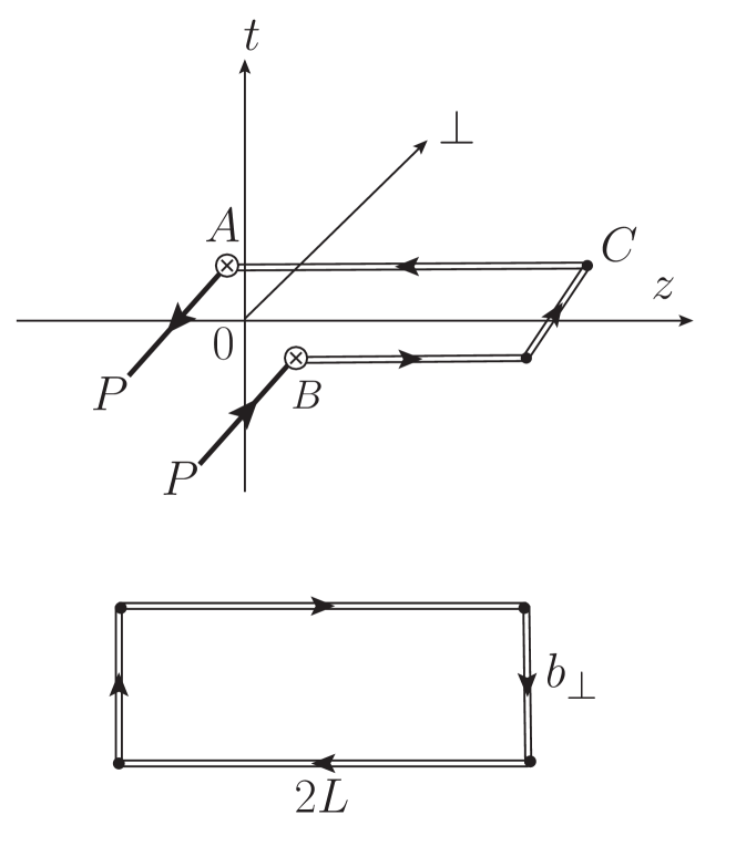
Figure 12: The quasi-TMDPDF (upper) and the Euclidean Wilson-loop $Z_{E}(2L,b_{\perp},\mu,0)$ (lower). In the figure, $A=\lambda n_{z}/2+\vec{b}_{\perp}/2$, $B=-\lambda n_{z}/2-\vec{b}_{\perp}/2$ and $C=Ln_{z}+{\vec{b}}_{\perp}$. The crosses denote the quark-link vertices.

The quasi-TMDPDFs defined above satisfy the following RGE Collins and Soper (1981); Ji et al. (2015b, 2019b)

$$\mu^{2}\frac{d}{d\mu^{2}}\ln\tilde{f}(x,b_{\perp},\mu,\zeta_{z})=\gamma_{F}(\alpha_{s}(\mu))\ ,$$ (209)

where $\gamma_{F}$ is the anomalous dimension for the heavy-to-light current in Sec. III.1. This is due to the fact that the quasi-TMDPDF, after the self-energy subtraction, contains only logarithmic UV divergences associated with quark-Wilson-line vertices. In the ${\overline{\rm MS}}$ scheme, the one-loop quasi-TMDPDF in an external quark state with momentum $(p^{z},0,0,p^{z})$ reads Ji et al. (2019a); Ebert et al. (2019b)

$$\tilde{f}(x,b_{\perp},\mu,\zeta_{z})=$$

$$1+\frac{\alpha_{s}C_{F}}{2\pi}F(x,\epsilon_{\tiny\mbox{IR}},b_{\perp},\mu)\theta(x)\theta(1-x)+\frac{\alpha_{s}C_{F}}{2\pi}\delta(1-x)$$

$$\times\Bigg{[}-\frac{1}{2}L_{b}^{2}+L_{b}\Big{(}\frac{5}{2}-L_{z}\Big{)}-\frac{3}{2}-\frac{1}{2}L_{z}^{2}+L_{z}\Bigg{]}\ ,$$ (210)

where $L_{z}=\ln(\zeta_{z}/\mu^{2})$. As expected, the $L$ dependence has been cancelled in the large $L$ limit.

As there is no light-like gauge-link in $\tilde{f}$, no additional rapidity regulator is needed. Instead, there is an explicit dependence on the hadron momentum (or energy), which is similar to the momentum RGE for collinear quasi-PDF. The momentum (rapidity) evolution equation for $\tilde{f}$ reads Collins and Soper (1981); Ji et al. (2015b, 2019b),

$$P^{z}\frac{d}{dP^{z}}\ln\tilde{f}(x,b_{\perp},\mu,\zeta_{z})\!=\!K(b_{\perp},\mu)\!+\!{\cal G}\Big{(}\frac{(P^{z})^{2}}{\mu^{2}}\Big{)}\ ,$$ (211)

where ${\cal G}(\zeta_{z}/\mu^{2})$ is perturbative and $K(b_{\perp},\mu)$ is the Collins-Soper kernel. A similar equation was proven for off-light-cone TMD-fragmentation functions in Collins and Soper (1981). From this equation, it is clear that a correct matching to $f^{\rm TMD}(x,b_{\perp},\mu,\zeta)$ with arbitrary $\zeta$ must include $K(b_{\perp},\mu)$ to compensate the $P^{z}$ dependence.

There is actually one more requirement for the matching: there is a rapidity scheme dependence which must be removed, since the quasi-TMDPDF can be viewed as defined with an off-light-cone regulator along the $z$ direction. To understand this dependence, let us consider $f$ again in the off-light-cone regularization, where there are rapidity divergences. The divergence is cancelled by the square root of an off-light-cone soft function $S_{\rm DY}(b_{\perp},\mu,Y,Y^{\prime})$, with $Y,Y^{\prime}$ being the rapidities of the off-light-cone space-like vectors $p\rightarrow p_{Y}=p-e^{-2Y}(p^{+})^{2}n$ and $n\rightarrow n_{Y^{\prime}}=n-e^{-2Y^{\prime}}p/(p^{+})^{2}$. Schematically, we have:

$$S_{\rm DY}(b_{\perp},\mu,Y,Y^{\prime})=\frac{{\rm tr}\langle 0|{\cal W}_{n_{Y^{\prime}}}(\vec{b}_{\perp}){\cal W}^{\dagger}_{p_{Y}}(\vec{b}_{\perp})|0\rangle}{N_{c}\sqrt{Z_{E}}\sqrt{Z_{E}}}\ ,$$ (212)

where ${\cal W}_{n_{Y^{\prime}}}(\vec{b}_{\perp})$ and ${\cal W}^{\dagger}_{p_{Y}}(\vec{b}_{\perp})$ are staple-shaped gauge-links in $n_{Y^{\prime}}$, $p_{Y}$ directions, respectively. $\sqrt{Z_{E}}$ is introduced to subtract the pinch pole singularities for the off-light-cone staple-shaped gauge-links. In terms of $\ln\rho^{2}=2(Y+Y^{\prime})$ sometimes we also write this soft function as $S_{\rm DY}(b_{\perp},\mu,\rho)$. At large $\rho$, we have

$$S_{\rm DY}(b_{\perp},\mu,Y,Y^{\prime})=e^{(Y+Y^{\prime})K(b_{\perp},\mu)+{\cal D}(b_{\perp},\mu)}+...\,.$$ (213)

We can perform a Lorentz boost of ${\cal W}_{n_{Y^{\prime}}}(\vec{b}_{\perp}){\cal W}^{\dagger}_{p_{Y}}(\vec{b}_{\perp})$ in Eq. (212) such that one of the gauge-links, say ${\cal W}_{n_{Y^{\prime}}}$, is boosted to the equal-time version ${\cal W}_{z}$ in $\tilde{f}$, whereas the other gauge-link ${\cal W}_{n_{Y}}$ is boosted to ${\cal W}_{n_{Y+Y^{\prime}}}$. The soft function becomes $S_{\rm DY}(b_{\perp},\mu,Y+Y^{\prime},0)$ which contains light-cone divergence for the $p_{Y+Y^{\prime}}$ direction, but is still the same $S_{\rm DY}(b_{\perp},\mu,Y,Y^{\prime})$ due to boost invariance. The square-root of the finite part $e^{{\cal D}(b_{\perp},\mu)}$ is exactly what is needed to cancel the rapidity-scheme dependence. We define the rapidity-independent part as the reduced soft function:

$$S_{r}(b_{\perp},\mu)\equiv e^{-{\cal D}(b_{\perp},\mu)}\,.$$ (214)

Based on the renormalization property of non-light-like Wilson-loops, the reduced soft function satisfies the RG equation

$$\mu^{2}\frac{d}{d\mu^{2}}\ln S_{r}(b_{\perp},\mu)=\Gamma_{S}(\alpha_{s})\,,$$ (215)

where $\Gamma_{S}$ is the constant part of the cusp-anomalous dimension at large hyperbolic cusp angle $Y+Y^{\prime}$ for the off-light-cone soft function:

$$\mu^{2}\frac{d}{d\mu^{2}}\ln S_{\rm DY}(b_{\perp},\mu,Y,Y^{\prime})$$

$$\qquad\qquad=-(Y+Y^{\prime})\Gamma_{\rm cusp}(\alpha_{s})-\Gamma_{S}(\alpha_{s})\,.$$ (216)

At one-loop level Ebert et al. (2019b),

$$S^{(1)}_{\rm DY}(b_{\perp},\mu,Y,Y^{\prime})=\frac{\alpha_{s}C_{F}}{2\pi}\big{[}2-2(Y+Y^{\prime})\big{]}L_{b}\ ,$$ (217)

and $\Gamma_{S}^{(1)}(\alpha_{s})=\alpha_{s}C_{F}/\pi$. Based on RGE, at two-loop level ${\cal D}(b_{\perp},\mu)$ can be predicted to be

$${\cal D}^{(2)}(b_{\perp},\mu)=c_{2}+\Gamma_{S}^{(2)}L_{b}-\frac{\alpha_{s}^{2}\beta_{0}C_{F}}{2\pi}L_{b}^{2}\ ,$$ (218)

where

$$\Gamma_{S}^{(2)}=-\frac{\alpha_{s}^{2}}{\pi^{2}}\Big{[}C_{F}C_{A}\big{(}-\frac{49}{36}+\frac{\pi^{2}}{12}-\frac{\zeta_{3}}{2}\big{)}+C_{F}N_{F}\frac{5}{18}\Big{]}$$

is the two-loop anomalous dimension for $S_{r}$ which can be extracted from Grozin et al. (2016), $\beta_{0}=-\left(\frac{11}{3}C_{A}-\frac{4}{3}N_{f}T_{F}\right)/(2\pi)$ is the coefficient of one-loop $\beta$-function, and $c_{2}$ is a constant to be determined by explicit calculation.

After taking into account the reduced soft function, we can now write down the matching formula between the quasi-TMDPDF and the scheme-independent TMDPDFJi et al. (2019b):

$$f^{\rm TMD}(x,b_{\perp},\mu,\zeta)$$ (219)

$$=H\left(\frac{\zeta_{z}}{\mu^{2}}\right)e^{-\ln(\frac{\zeta_{z}}{\zeta})K(b_{\perp},\mu)}\tilde{f}(x,b_{\perp},\mu,\zeta_{z})S_{r}^{\frac{1}{2}}(b_{\perp},\mu)+...\ ,$$

where the power-corrections of order ${\cal O}\left(\Lambda_{\rm QCD}^{2}/\zeta_{z},M^{2}/(P^{z})^{2},1/(b^{2}_{\perp}\zeta_{z})\right)$. The above relation except for the definition of $S_{r}(b_{\perp},\mu)$ was argued to hold in Ebert et al. (2019b), where the unknown function $g_{q}^{S}$ in Eq. (5.3) should be identified as the reduced soft function here; it has also been confirmed recently in Vladimirov and Schäfer (2020).

We now explain the individual factors of the formula.

1. The factor $H(\zeta_{z}/\mu^{2})$ is the perturbative matching kernel, which is a function of $\zeta_{z}/\mu^{2}=(2xP^{z})^{2}/\mu^{2}$. The kernel is responsible for the large logarithms of $P^{z}$ generated by the ${\cal G}(\zeta_{z}/\mu^{2})$ term of the momentum RG equation. Unlike the case of quasi-PDFs, the momentum fractions of the quasi-TMDPDF and the TMDPDF are the same. This is due to the fact that at leading power in $1/\zeta_{z}$ expansion, the $k_{\perp}$ integral is naturally cut off by the transverse separation around $k_{\perp}\sim 1/b_{\perp}\ll P^{z}$. Therefore, the momentum fraction can only be modified by collinear modes for which there are no distinction between $x=k^{z}/P^{z}$ and $x=k^{+}/P^{+}$. In comparison, for the $\vec{k}_{\perp}$ integrated quasi-PDF, the $k_{\perp}\geq P^{z}$ region leads to non-trivial $x$ dependence outside the physical region. This is also consistent with the fact that the momentum evolution equation for quasi-TMDPDF is local in $x$ instead of being a convolution.

2. The factor $\exp\big{[}\ln(\frac{\zeta_{z}}{\zeta})K(b_{\perp},\mu)\big{]}$ is the part involving the Collins-Soper evolution kernel. From the momentum evolution equation, it is clear that at large $P^{z}$ there are logarithms of the form $K(b_{\perp},\mu)\ln\frac{\zeta_{z}}{\mu^{2}}$ with $\zeta_{z}$ being the natural Collins-Soper scale. Therefore, to match to the TMDPDF at arbitrary $\zeta$, a factor $\exp\big{[}\ln(\frac{\zeta_{z}}{\zeta})K(b_{\perp},\mu)\big{]}$ is required to compensate the difference. An important implication of this property is that one can obtain the Collins-Soper kernel $K(b_{\perp},\mu)$ by constructing the ratio of quasi-TMDPDFs at two different momenta or $\zeta_{z}$’s Ebert et al. (2019a),

   $$\ \ \quad\frac{\tilde{f}(x,b_{\perp},\mu,\zeta_{z,1})}{\tilde{f}(x,b_{\perp},\mu,\zeta_{z,2})}=\frac{H\left(\frac{\zeta_{z,2}}{\mu^{2}}\right)}{H\left(\frac{\zeta_{z,1}}{\mu^{2}}\right)}\left(\frac{\zeta_{z,1}}{\zeta_{z,2}}\right)^{K(b_{\perp},\mu)}\ .$$ (220)

   Thus given the $\tilde{f}$’s at the two rapidity scales, the Collins-Soper kernel $K(b_{\perp})$ can be obtained.

Combining the RGEs of the quasi-TMDPDF $\tilde{f}$, reduced soft function $S_{r}$ and physical TMDPDF $f^{\rm TMD}$, we obtain the RGE of the matching kernel $H\left(\frac{\zeta_{z}}{\mu^{2}}\right)$ Ji et al. (2019b),

$$\mu^{2}\frac{d}{d\mu^{2}}\ln H^{-1}\left(\frac{\zeta_{z}}{\mu^{2}}\right)=\frac{1}{2}\Gamma_{\rm cusp}(\alpha_{s})\ln\frac{\zeta_{z}}{\mu^{2}}\!+\!\frac{\gamma_{C}(\alpha_{s})}{2}\ ,$$ (221)

where $\gamma_{C}(\alpha_{s})=2\gamma_{F}(\alpha_{s})+\Gamma_{S}(\alpha_{s})+2\gamma_{H}(\alpha_{s})$. The matching kernel is closely related to the perturbative part of the rapidity evolution kernel ${\cal G}\left(\frac{\zeta_{z}}{\mu^{2}}\right)$ through

$$2\zeta_{z}\frac{d}{d\zeta_{z}}\ln H^{-1}\left(\frac{\zeta_{z}}{\mu^{2}}\right)={\cal G}\left(\frac{\zeta_{z}}{\mu^{2}}\right)\ .$$ (222)

Again, we can see that the anomalous dimension of ${\cal G}\left(\frac{\zeta_{z}}{\mu^{2}}\right)$ is $\Gamma_{\rm cusp}(\alpha_{s})$.

It is convenient to write $H$ in the exponential form, $H=e^{-h}$. Collecting all the above results, one obtains at one-loop level Ji et al. (2019a); Ebert et al. (2019b)

$$h^{(1)}\left(\frac{\zeta_{z}}{\mu^{2}}\right)=\frac{\alpha_{s}C_{F}}{2\pi}\left(-2+\frac{\pi^{2}}{12}-\frac{L_{z}^{2}}{2}+L_{z}\right)\ .$$ (223)

Similar as before, the two loop contribution $h^{(2)}$ is predicted to be

$$h^{(2)}\left(\frac{\zeta_{z}}{\mu^{2}}\right)=c^{\prime}_{2}-\frac{1}{2}\left(\gamma^{(2)}_{C}-\alpha_{s}^{2}\beta_{0}c_{1}\right)\ln\frac{\zeta_{z}}{\mu^{2}}$$ (224)

$$-\frac{1}{4}\left(\Gamma^{(2)}_{\rm cusp}-\frac{\alpha_{s}^{2}\beta_{0}C_{F}}{2\pi}\right)\ln^{2}\frac{\zeta_{z}}{\mu^{2}}-\frac{\alpha_{s}^{2}\beta_{0}C_{F}}{24\pi}\ln^{3}\frac{\zeta_{z}}{\mu^{2}}\ ,$$

where $c_{1}=\frac{C_{F}}{2\pi}\left(-2+\frac{\pi^{2}}{12}\right)$ and $c^{\prime}_{2}$ is again a constant to be determined in perturbation theory at two-loop level.

Finally, we compare the current formulation with previous approaches to lattice TMDPDF. First, we comment on the developments in Hagler et al. (2009); Musch et al. (2011, 2012); Engelhardt et al. (2016); Yoon et al. (2017) in which the $x$-moments of TMDPDF are extracted from ratio of quasi-TMDPDF. From Eq. (219), it is clear that both the matching kernel $H$ and the exponential factor of Collins-Soper kernel depends on $x$ non-trivially. Therefore, simply taking the ratio of moments for quasi-TMDPDF will not be sufficient to reproduce the same ratio for TMDPDF, although the soft function does cancel. This observation is also made recently in Ref. Ebert et al. (2020a). Second, the quasi-TMDPDF defined with the naive rectangle-shaped soft function, i.e. $Z_{E}$, is $\tilde{f}$ in Eq. (205), so it is obvious that it still needs the reduced soft function $S_{r}$ to be matched to $f^{\rm TMD}$. As for the other proposal in Ji et al. (2015b); Ebert et al. (2019b), it replaces $Z_{E}$ in $\tilde{f}$ with $S_{\rm bent}$ which is the vacuum matrix element of a spacelike bent-shaped Wilson loop with angle $\pi/2$ at each junction, and does not include the function $S^{1\over 2}_{r}$ in Eq. (219). Although $\sqrt{S_{\rm bent}/Z_{E}}$ agrees with $S_{r}^{-1\over 2}$ at one-loop order Ji et al. (2019a); Ebert et al. (2019b), it is expected to be different at higher orders. In fact, for the anomalous dimension $\Gamma_{\pi\over 2}$ defined through

$$\Gamma_{\frac{\pi}{2}}(\alpha_{s})\equiv\mu^{2}\frac{d}{d\mu^{2}}\ln\left(\frac{S_{\rm bent}(L,b_{\perp},\mu)}{Z_{E}(2L,b_{\perp},\mu)}\right)\,,$$ (225)

it starts to deviate from $\Gamma_{S}(\alpha_{s})$ at two-loop order Grozin et al. (2016), as

$$-\Gamma_{S}(\alpha_{s}) =\frac{\alpha_{s}C_{F}}{\pi}$$ (226)

$$+\frac{\alpha_{s}^{2}}{\pi^{2}}\left[C_{F}C_{A}\left(-\frac{49}{36}+\frac{\pi^{2}}{12}-\frac{\zeta_{3}}{2}\right)+C_{F}N_{F}\frac{5}{18}\right]\,,$$

$$\Gamma_{\frac{\pi}{2}}(\alpha_{s}) =\frac{\alpha_{s}C_{F}}{\pi}$$ (227)

$$+\frac{\alpha_{s}^{2}}{\pi^{2}}\left[C_{F}C_{A}\left(-\frac{49}{36}+\frac{\pi^{2}}{24}\right)+C_{F}N_{F}\frac{5}{18}\right]\,.$$

In the equation, $\zeta_{3}=\sum_{n=1}^{\infty}(1/n^{3})\neq\pi^{2}/12$, therefore the two anomalous dimensions are different. The differences in the anomalous dimension will result in different logarithmic behaviors in $b_{\perp}$, as the soft functions are dimensionless and depend on $b_{\perp}$ and $\mu$ only. At large $b_{\perp}$, it will lead to different IR physics that cannot be controlled by perturbation theory.

Combining the reduced soft function and the quasi-TMDPDF, one can effectively factorize the DY cross section,

$$\sigma=\int dx_{A}dx_{B}d^{2}b_{\perp}e^{i\vec{Q}_{\perp}\cdot\vec{b}_{\perp}}\hat{\sigma}(x_{A},x_{B},Q^{2},\mu)$$

$$\times\tilde{f}(x_{A},b_{\perp},\mu,\zeta_{A})\tilde{f}(x_{B},b_{\perp},\mu,\zeta_{B})S_{r}(b_{\perp},\mu)\ .$$ (228)

where all non-perturbative quantities do not involve the light cone, and can be calculated on lattice.

Spin-dependent TMDPDFs are also physically important. They can be computed using LaMET theory Ebert et al. (2020a). Again one can define quasi distributions just like the spin-independent ones. For a general proton target $|PS\rangle$ and the general spin structure $\Gamma$ of the parton, the parent TMDPDF can be defined as :

$$f_{[\Gamma]}^{\rm TMD}(x,\vec{k}_{\perp},\mu,\zeta)=\frac{1}{2P^{+}}\int\frac{d\lambda}{2\pi}\int\frac{d^{2}\vec{b}_{\perp}}{(2\pi)^{2}}e^{-i\lambda x+i\vec{k}_{\perp}\cdot\vec{b}_{\perp}}$$

$$\times\lim_{\delta^{-}\rightarrow 0}\frac{\langle PS|\bar{\psi}(\lambda n+\vec{b}_{\perp})\Gamma\,{\cal W}_{n}(\lambda n+\vec{b}_{\perp})|_{\delta^{-}}\psi(0)|PS\rangle}{\sqrt{S(b_{\perp},\mu,\delta^{-}e^{2y_{n}},\delta^{-})}}\,,$$ (229)

where the $\zeta=2(P^{+})^{2}e^{2y_{n}}$ is the rapidity scale, see Sec. V for more detail of the soft function subtraction. The individual spin-dependent TMD distributions can then be obtained through Lorentz decompositions  Tangerman and Mulders (1995); Ralston and Soper (1979); Mulders and Tangerman (1996):

$$f_{[\gamma^{+}]}^{\rm TMD} =f_{1}-\frac{\epsilon^{ij}k^{i}S^{j}_{\perp}}{M}f_{1T}^{\perp}\,,$$ (230)

$$f_{[\gamma^{+}\gamma_{5}]}^{\rm TMD} =S^{+}g_{1}+\frac{\vec{k}_{\perp}\cdot\vec{S}_{\perp}}{M}g_{1T}\,,$$ (231)

$$f_{[i\sigma^{i+}\gamma_{5}]}^{\rm TMD} =S_{\perp}^{i}h_{1}+\frac{(2k^{i}k^{j}-\vec{k}_{\perp}^{2}\delta^{ij})S^{j}_{\perp}}{2M^{2}}h_{1T}^{\perp}$$

$$\qquad+\frac{S^{+}k^{i}}{M}h_{1L}^{\perp}+\frac{\epsilon^{ij}k^{j}}{M}h_{1}^{\perp}\,,$$ (232)

where we suppress the arguments $(x,\vec{k}_{\perp},\mu,\zeta)$ in all distributions; $f_{1}$, $g_{1}$, and $h_{1}$ are unpolarized, helicity and transversity TMDPDFs, respectively; the indices $i$ and $j$ are in transverse space of $\vec{k}_{\perp}$; $S^{+}$ and $S^{i}_{\perp}$ are longitudinal and transverse spin components.

Note that the Sivers function $f^{\perp}_{1T}$ Sivers (1990) and the Boer-Mulders function $h^{\perp}_{1}$ Boer and Mulders (1998) are $T$-odd. The orientation of the gauge-link have important effects on these two functions Collins (2002, 2011a), such that they change sign between the DY and SIDIS processes. In the light-cone gauge, these contributions arise from the transversal gauge-link at infinities Belitsky et al. (2003). They are related to the phenomenologically interesting single transverse-spin asymmetry Boer and Mulders (1998); Efremov et al. (2005); Collins et al. (2006, 2005).

V.3 Off-light-cone Soft Function

In previous subsections, the soft function has been introduced to define rapidity-scheme-independent TMDPDFs. The major motivation of introducing the soft function is to capture nonperturbative effects due to soft-gluon radiations from fast moving color-charges. For many inclusive processes the soft radiations cancel in the total cross section, but for certain processes where a small transverse momentum is measured, such cancellation can be incomplete and result in measurable consequences. In such cases, the TMD soft function is introduced to account for the soft-gluon effects and appears in factorization theorems for the Drell-Yan (DY) process Collins et al. (1985b, 1988) and semi-inclusive DIS (SIDIS) Ji et al. (2005, 2004).

To calculate the TMD physics nonperturbatively, formulating a Euclidean version of the soft function is critical. Since the soft function in fact is a cross section and hence real and positive, it satisfies the necessary condition for a Monte Carlo simulation. In this subsection, we present an approach to calculate it in heavy-quark effective theory (HQET) Ji et al. (2020a). There is also another method proposed to extract the reduced soft function $S_{r}$ from a light-meson form factor Ji et al. (2020a), where many subtleties of HQET can be avoided. The first lattice calculation of the reduced soft function based on the light-meson formalism has been performed in the recent work Zhang et al. (2020a).

Due to the different space-time pictures of the DY and SIDIS processes, the soft functions for the two processes also differ from each other as shown in Fig. 11. To define the soft function, one also needs to specify a time-ordering prescription. Since it is a cross section, it involves a time order and an anti-time order (or cut diagrams). However, in the light-cone limit, the time order does not matter. What really matters is the rapidity regularization scheme. It has been proven for the $\delta$ regulator in  Vladimirov (2018) that the time ordering is not quite relevant up to overall phase factors, and the soft functions for the two processes are equal. The method therein can be modified to apply to the off-light-cone scheme too. Therefore, our first step is to convert the cut-diagrams into Feynman diagrams by imposing just the single time order. In this way, the soft function can be viewed as a scattering amplitude.

In the off-light-cone scheme, there are further complications caused by the space-like or time-like choices for off-light-cone vectors. Fortunately, one can show that in the light-cone limit, the space-like and time-like choices are equivalent up to overall phase factors Ji et al. (in preparation). Thus we will use the notation $S(b_{\perp},\mu,Y,Y^{\prime})$ to denote a generic off-light-cone soft function that satisfies our demands.

With these in mind, we show that the off-light-cone soft function $S(b_{\perp},\mu,Y,Y^{\prime})$ is equivalent to an equal-time form factor of fast-moving color sources and can be formulated on the Euclidean lattice. From the matching formula Eq. (219) in the last subsection, once the off-light-cone soft function is known, we can combine it with the lattice calculated quasi-TMDPDF to obtain the physical TMDPDF. Therefore, the cross section of DY processes in the low transverse-momentum region Collins et al. (1985b) becomes predictable from first principles Ji et al. (2020a).

To begin with, we define the scattering amplitude of a Wilson loop as shown in Fig. 13:

$$W(t,t^{\prime},b_{\perp},Y,Y^{\prime})$$

$$=\frac{1}{N_{c}}{\rm Tr\,}\langle 0|{\cal T}\left[{\cal W}^{\dagger}_{v^{\prime}}(\vec{b}_{\perp},t^{\prime}){\cal W}_{v}(\vec{b}_{\perp},t)\right]|0\rangle$$ (233)

where $|0\rangle$ is the QCD vacuum state and $N_{c}$ is number of colors and ${\rm Tr}$ is the color-trace. Timelike four-vectors $v^{\mu}=\gamma(1,\beta,\vec{0}_{\perp})$ and $v^{\prime\mu}=\gamma^{\prime}(1,-\beta^{\prime},\vec{0}_{\perp})$ approach the lightcone as $\beta$ and $\beta^{\prime}\to 1$. The rapidity $Y$ and the speed $\beta$ are related through $\beta={\rm tanh}Y$, in terms of the light-cone vectors $p$ and $n$, the velocities read $v=\frac{e^{Y}}{\sqrt{2}}\left(\frac{p}{p^{+}}+e^{-2Y}p^{+}n\right)$ and $v^{\prime}=\frac{e^{Y}}{\sqrt{2}}\left(e^{-2Y}\frac{p}{p^{+}}+p^{+}n\right)$. The ${\cal W}_{v}(\vec{b}_{\perp},t)$ is a staple-shaped gauge-link along $v$ direction similar to those defined in Eqs. (183) and (206). $t$ and $t^{\prime}$ are the lengths of the $t$-components of the staples. The single time-order prescription for $S$ allows physical interpretation as a chronological process.

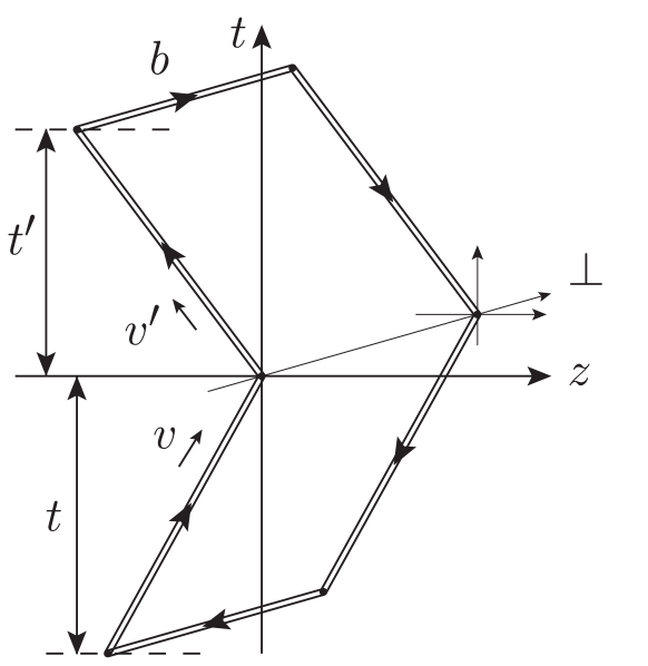
Figure 13: The Wilson-loop ${\cal W}$ showing a pair of quark and antiquark scattering at $t=0$.

Similar to the quasi-TMDPDF, the Wilson-loop in Eq. (V.3) contains pinch-pole singularities associated to time evolution of initial and final states at large $t$ and $t^{\prime}$. Therefore, we need to subtract them out in Eq. (V.3) with rectangular Wilson-loops Collins (2008); Ji et al. (2019a). This leads to an off-light-cone realization of the soft function:

$$S(b_{\perp},\mu,Y,Y^{\prime})$$

$$=\lim_{\begin{subarray}{c}t\to\infty\\ t^{\prime}\to\infty\end{subarray}}\frac{W(t,t^{\prime},b_{\perp},\mu,Y,Y^{\prime})}{\sqrt{Z(2t,b_{\perp},\mu,Y)Z(2t^{\prime},b_{\perp},\mu,Y^{\prime})}}\ ,$$ (234)

where $Z(2t,b_{\perp},Y)$ is the vacuum expectation value of rectangular Wilson loop which is similar to $W$ by setting $v^{\prime}=v$ and $t^{\prime}=t$, i.e. $Z(2t,b_{\perp},Y)=W(t,t,b_{\perp},Y,-Y)$. The factor $Z$ has a clear physical interpretation: It can be viewed as the wave function renormalization for incoming or outgoing color sources. After the subtraction through $Z$, the only remaining UV divergences for $S(b_{\perp},\mu,Y,Y^{\prime})$ are the cusp divergences with hyperbolic angle $Y+Y^{\prime}$.

We should mention that a more common definition of the soft function $S_{\rm DY}(b_{\perp},\mu,Y,Y^{\prime})$ for the DY process was proposed in Collins (2011b, a). The space-like vectors $u^{\mu}=\gamma(\beta,1,0,0)$ and $u^{\prime\mu}=\gamma^{\prime}(-\beta^{\prime},1,0,0)$ were chosen instead of time-like $v$ and $v^{\prime}$ to define the soft function for the DY process. This soft function has already been defined in the last subsection in Eq. (212). $u$ and $u^{\prime}$ are equal to $p_{Y}$, $n_{Y^{\prime}}$ up to overall normalization factors.

While $S$ and $S_{\rm DY}$ are defined differently, we can show that

$$S(b_{\perp},\mu,Y,Y^{\prime})=S_{\rm DY}(b_{\perp},\mu,Y,Y^{\prime})$$ (235)

using analyticity property Ji et al. (in preparation). Here we focus on $S$ in Eq. (V.3), which has a simple Euclidean realization.

After defining the soft function $S$, we now show that it is equal to a form factor. In HQET, the propagator of a color source is equivalent to a gauge-link along its moving direction. Thus $W(t,t^{\prime},b_{\perp},\mu,Y,Y^{\prime})$ can be expressed by fields in HQET with the Lagrangian

$${\cal L_{\rm HQET}}=Q_{v}^{\dagger}(x)(iv\cdot D)Q_{v}(x)+\bar{Q}_{v}^{\dagger}(x)(iv\cdot D)\bar{Q}_{v}(x)\ ,$$ (236)

where $Q_{v}$ and $\bar{Q}_{v}$ are quark and anti-quark in the fundamental and anti-fundamental representations, respectively; $v^{\mu}=\gamma(1,\beta,\vec{0}_{\perp})$ is the four velocity; $D$ is the covariant derivative. Note that quarks in HQET can be viewed as color sources. If the gluon soft function is considered, the heavy quarks should be in the adjoint representation.

In HQET, a color-singlet heavy-quark pair separated by $\vec{b}$ generates a heavy quark potential $V(|\vec{b}|)$ in the ground state, and the spectrum includes a gapped continuum above it. The state can also have a residual momentum $\delta\vec{P}$, which is arbitrary due to reparameterization invariance Luke and Manohar (1992); Manohar and Wise (2000), and for simplicity we always consider $\delta\vec{P}=0$. When the sources move with a velocity $v$, the ground state can be labeled by $|\overline{Q}Q,\vec{b},\delta\vec{P}\rangle_{v}$, where the residue momentum $\delta\vec{P}=\vec{P}_{\rm total}-2m_{Q}\gamma\vec{\beta}$ is the difference between the total momentum $\vec{P}_{\rm total}$ and the kinetic momentum of the heavy-quarks. The residual energy of the state is $E=\gamma^{-1}V(|\vec{b}_{\perp}|)+\vec{\beta}\cdot\delta\vec{P}$.

Consider a process with incoming and outgoing states being heavy-quark pairs separated by ${\vec{b}}_{\perp}$ and at velocity $v$ and $v^{\prime}$, respectively. Such a state is created by the interpolating fields

$${\cal O}_{v}(t,{\vec{b}}_{\perp})=\int d^{3}\vec{r}\,Q_{v}^{\dagger}(t,\vec{r}\,){\cal U}(\vec{r},\vec{r}\,^{\prime},t)\bar{Q}_{v}^{\dagger}(t,\vec{r}\,^{\prime})\ ,$$ (237)

where $\vec{r}\,^{\prime}=\vec{r}+\vec{b}_{\perp}$ and ${\cal U}(\vec{r},\vec{r}\,^{\prime},t)$ is a gauge-link connecting $\vec{r}\,^{\prime}$ to $\vec{r}$ at time $t$. The heavy-quark pair created by ${\cal O}_{v}$ is forced to be at relative separation $\vec{b}_{\perp}$ and to have vanishing residual momentum $\delta\vec{P}=0$. Between the incoming and outgoing states, a product of two local equal-time operators

$$J(v,v^{\prime},\vec{b}_{\perp})=\bar{Q}^{\dagger}_{v^{\prime}}(\vec{b}_{\perp})\bar{Q}_{v}(\vec{b}_{\perp})Q_{v^{\prime}}^{\dagger}(0)Q_{v}(0)$$ (238)

is inserted at $t=0$. Then $W$ can be expressed in terms of HQET propagators which are gauge-links in the $v,v^{\prime}$ directions. After integrating out the heavy-quark fields, we obtain up to an overall volume factor Ji et al. (2020a)

$$W(t,t^{\prime},b_{\perp},\mu,Y,Y^{\prime})$$ (239)

$$=\frac{1}{N_{c}}\langle 0|{\cal O}^{\dagger}_{v^{\prime}}(t^{\prime},{\vec{b}}_{\perp})J(v,v^{\prime},\vec{b}_{\perp}){\cal O}_{v}(-t,\vec{b}_{\perp})|0\rangle$$

$$\xrightarrow[\begin{subarray}{c}t\to\infty\\ t^{\prime}\to\infty\end{subarray}]{}\frac{1}{N_{c}}\Phi^{\dagger}(b_{\perp},\mu)S(b_{\perp},\mu,Y,Y^{\prime})\Phi(b_{\perp},\mu)e^{-iE^{\prime}t^{\prime}-iEt}\ ,$$

where

$$\Phi(b_{\perp},\mu) =\lim_{T\to\infty}{}_{v}\langle\overline{Q}Q,\vec{b}_{\perp}|{\cal O}_{v}(T,\vec{b}_{\perp})|0\rangle\,,$$ (240)

$$S(b_{\perp},\mu,Y,Y^{\prime}) ={{}_{v^{\prime}}}\langle\overline{Q}Q,\vec{b}_{\perp}|J(v,v^{\prime},\vec{b}_{\perp})|\overline{Q}Q,\vec{b}_{\perp}\rangle_{v}\ .$$

In the last line of Eq. (239), we have inserted a complete set of heavy-quark pair states before and after $J$. At large $t$ and $t^{\prime}$, the contribution from the continuum spectrum is damped out due to the Riemann-Lebesgue lemma Zuazo (2001), while the contribution from $|\overline{Q}Q,\vec{b}_{\perp},\delta\vec{P}=0\rangle_{v}$ with residual energy $E=\gamma^{-1}V(|\vec{b}_{\perp}|)$ survives. As a result we obtain Eqs. (239)—(240), where we have omitted the state label $\delta\vec{P}=0$ for simplicity. Alternatively, we can also give $t$ and $t^{\prime}$ a small negative imaginary part, which is consistent with the time order, to damp out all states except $|\overline{Q}Q,\vec{b}_{\perp}\rangle_{v}$ at large $t$ and $t^{\prime}$. Note that $\Phi(\vec{b}_{\perp},\mu)$ is independent of $Y$ because it is boost invariant.

Similarly, $Z$ can also be formulated in HQET as

$$Z(2t,b_{\perp},Y) =\frac{1}{N_{c}}\langle 0|{\cal O}^{\dagger}_{v^{\prime}}(t,{\vec{b}}_{\perp}){\cal O}_{v}(-t,\vec{b}_{\perp})|0\rangle$$

$$\xrightarrow[\begin{subarray}{c}t\to\infty\end{subarray}]{}\frac{1}{N_{c}}\Phi^{\dagger}({\vec{b}}_{\perp},\mu)\Phi({\vec{b}}_{\perp},\mu)e^{-2iEt}\,,$$ (241)

whose $t$-component has length $2t$. The $Y$ dependence of $Z$ is implicit in the energy $E$. Combining Eqs. (239) and (V.3), we obtain $S$ defined in Eq. (V.3). We emphasize that Eq. (V.3) can be seen as a LSZ reduction formula, in which we amputate the external heavy-quark pair states $|\overline{Q}Q,{\vec{b}}_{\perp}\rangle_{v}$.

Being an equal-time observable, $S(b_{\perp},\mu,Y,Y^{\prime})$ can be straightforwardly realized in Euclidean time as:

$$S(b_{\perp},\mu,Y,Y^{\prime})$$ (242)

$$=\lim_{\begin{subarray}{c}T\to\infty\\ T^{\prime}\to\infty\end{subarray}}\frac{W_{E}(T,T^{\prime},b_{\perp},\mu,Y,Y^{\prime})}{\sqrt{Z_{E}(2T,b_{\perp},\mu,Y)Z_{E}(2T^{\prime},b_{\perp},\mu,Y^{\prime})}}\ ,$$

where the subscript $E$ indicates the quantity is defined in Euclidean time, with corresponding variables $T$ and $T^{\prime}$. Due to boost invariance, the factor $Z_{E}(T,b_{\perp},\mu,Y)$ relates to the rectangular Wilson-loop defined in Eq. (208) along the $n_{z}$ direction through the relation $Z_{E}(2T,b_{\perp},\mu,Y)=Z_{E}(2\gamma^{-1}T,b_{\perp},0)$. The relevant matrix elements are now calculated by a lattice version of HQET with the Lagrangian Aglietti (1994); Hashimoto and Matsufuru (1996); Horgan et al. (2009)

$${\cal L}_{{\rm HQET}}^{E}$$ (243)

$$=Q_{v}^{\dagger}(x)(i\tilde{v}\cdot D_{E})Q_{v}(x)+\bar{Q}_{v}^{\dagger}(x)(i\tilde{v}\cdot D_{E})\bar{Q}_{v}(x)\ ,$$

where the subscript $E$ denotes the Euclidean space, $i\tilde{v}\cdot D_{E}=\gamma(D^{\tau}-i\beta)D^{z}$ with $\tilde{v}^{\mu}=\gamma(-i,-\beta,\vec{0}_{\perp})$. We have explicitly verified Eq. (242) in Euclidean perturbation theory to the one-loop order.

The soft function cannot be calculated on the lattice by simply replacing the Minkowskian gauge-links in Eq. (V.3) with a finite number of Euclidean gauge-links. Through HQET, we find a time-independent formulation of the soft function, which opens up the possibility of direct lattice calculations.

V.4 Light-Front Wave-Function Amplitudes And Soft Function from Meson Form Factor

Light-front quantization (LFQ) or formalism is a natural language for parton physics in which partons are made manifest at all stages of calculations. It favors a Hamiltonian approach to QCD like for a non-relativistic quantum mechanical system, i.e., to diagonalize the Hamiltonian

$$\hat{P}^{-}|\Psi_{n}\rangle=\frac{M^{2}_{n}+{\vec{P}_{\perp}}^{2}}{2P^{+}}|\Psi_{n}\rangle\ ,$$ (244)

to obtain wave functions for the QCD bound states Brodsky et al. (1998). The light-front wave functions (LFWFs) thus obtained can, in principle, be used to calculate all the partonic densities and correlations functions. Moreover, like in condensed matter systems, knowing quantum many-body wave-functions allows one to understand interesting aspects of quantum coherence and entanglement, as well as the fundamental nature of quantum systems. Therefore, a practical realization of light-front quantization program clearly would be a big step forward in understanding the fundamental structure of the proton.

However, from a field theory point of view, wave functions are not the most natural objects to consider due to the non-trivial vacuum, UV divergences as well as the requirement of Lorentz symmetry, according to which the space and time should be treated on equal footing. The proton or other hadrons are excitations of the QCD vacuum which by itself is very complicated because of the well-known phenomena of chiral symmetry breaking and color confinement. To build a proton on top of this vacuum, one naturally has a question of what part of the wave-function reflects the property of the proton and what reflects the vacuum: It is the difference that yields the properties of the proton that are experimentally measurable. There is no clean way to make this separation unless one builds the proton out of elementary excitations or quasi-particles that do not exist in the vacuum, as often done in condensed matter systems.

The partons in the IMF avoids the above problems to a certain extent. In fact, due to the kinematic effects, in the IMF all partons in the vacuum have longitudinal momentum $k^{+}=0$, and to some degree of accuracy, the proton is made of partons with $k^{+}\neq 0$. This natural separation of degrees of freedom (DOF) is particularly welcome, making a wave-function description of the proton more natural and interesting in IMF than in any other frame.

To implement the above DOF separation, one possibility is to assume triviality of the light-front vacuum. The question that to what extent this holds has been continuously debated over the years. One knows a priori that in relativistic QFT, the vacuum state is boost invariant and frame-independent. In fact, it was proven in Nakanishi and Yabuki (1977); Nakanishi and Yamawaki (1977) that not only the vacuum can not be trivial, even the Green’s functions of the full theory cannot pose generic meaningful restrictions to the null-planes $\xi^{+}=c$. In fact, the vacuum zero modes do contain non-trivial dynamics and contribute to the properties of the proton Ji (2020). Nevertheless, one can adopt an effective theory point of view to simply cut off the zero-modes and relegate their physics to renormalization constants. In some simple cases, these zero-modes can be treated explicitly Heinzl et al. (1991); Yamawaki (1998).

By imposing an IR cut-off on the $k^{+}\geq\epsilon$ in the effective Hilbert space, all physics below $k^{+}=\epsilon$ are taken into account through renormalization constants. We then obtain an effective LF theory with trivial vacuum,

$$a_{k\lambda}|0\rangle=b_{p\sigma}|0\rangle=d_{p\sigma}|0\rangle=0\ .$$ (245)

where $|0\rangle$ is the vacuum of LFQ. Therefore, the proton can be expanded in terms of the superposition of Fock states in the LF gauge $A^{+}=0$ Brodsky et al. (1998),

$$|P\rangle=\sum_{n=1}^{\infty}\int d\Gamma_{n}\psi^{0}_{n}(x_{i},\vec{k}_{i\perp})\prod a^{\dagger}_{i}(x_{i},\vec{k}_{i\perp})|0\rangle\ .$$ (246)

where $a^{\dagger}$ are generic quarks and gluon quanta on the light-front, the phase-space integral reads $d\Gamma_{n}=\prod\frac{dk^{+}d^{2}k_{\perp}}{2k^{+}(2\pi)^{3}}$. The $\psi_{n}(x_{i},\vec{k}_{i\perp})$ are LFWF amplitudes or simply WF amplitudes, where $x_{i}$ to denote the set of momentum fractions from $x_{1}$ to $x_{n}$. They are a complete set of non-perturbative quantities which describe the partonic landscape of the proton. The above amplitudes can in principle be calculated through Hamiltonian diagonalization. However, as explained in Sec. II.1, a direct systematic solution in LFQ is impractical.

LaMET offers an alternate route to calculate these WF amplitudes. Thanks to the triviality of the vacuum after the truncation $k^{+}\geq\epsilon$, they can then be written in terms of the invariant matrix elements by inverting the above expansion,

$$\psi^{0}_{n}(x_{i},\vec{k}_{i\perp})=\langle 0|\prod a_{i}(x_{i},\vec{k}_{i\perp})|P\rangle\ .$$ (247)

After properly restoring gauge-invariance and imposing regularizations, they become the matrix elements of light-cone correlators, the same type as those in the TMDPDFs. Therefore, the LaMET method applies to them, which allows one to effectively obtain the results of light-front quantization through instant quantization in a large momentum frame.

To realize the goal, the LFWF amplitudes also need a rapidity renormalization, as in the case of TMDPDFs. In this section, we explain how the reduced soft function $S_{r}$ can be obtained by combining the LFWF amplitudes and a special light-meson form factor, instead of as the form factor in HQET discussed in the previous section. A lattice calculation based on the light-meson framework has been performed in Zhang et al. (2020a).

Let us consider the following form factor of a pseudoscalar light-meson state with constituents $\overline{\psi}\eta$,

$$F(b_{\perp},P,P^{\prime},\mu)=\langle P^{\prime}|\overline{\eta}(\vec{b}_{\perp})\Gamma^{\prime}\eta(\vec{b}_{\perp})\overline{\psi}(0)\Gamma\psi(0)|P\rangle$$ (248)

where $\psi$ and $\eta$ are light quark fields of different flavors; $P^{\mu}=(P^{t},0,0,P^{z})$ and $P^{\prime\mu}=(P^{t},0,0,-P^{z})$ are two large momenta which approach two opposite light-like directions in the limit $P^{z}\to\infty$; $\Gamma$ and $\Gamma^{\prime}$ are Dirac gamma matrices, which can be chosen as $\Gamma=\Gamma^{\prime}=1$, $\gamma_{5}$ or $\gamma_{\perp}$ and $\gamma_{\perp}\gamma_{5}$, so that the quark fields have leading components on the respective light-cones.

At large momentum, the form factor factorizes through TMD factorization into LFWF amplitudes. To motivate the factorization, we need to consider the leading region of IR divergences in a similar way for SIDIS and Drell-Yan Ji et al. (2005); Collins (2011b), and the result is shown in Fig. 14.

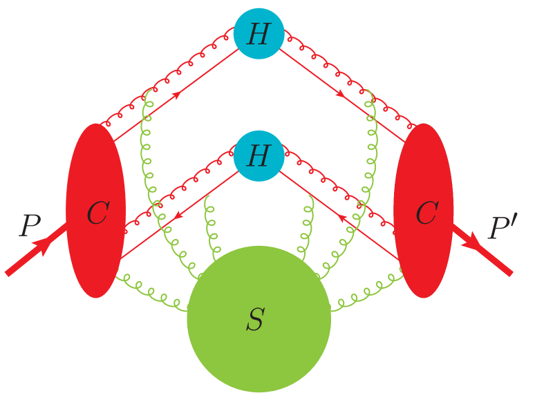
Figure 14: The reduced diagram for the large-momentum form factor $F$ of a meson. Two $H$ denote the two hard cores separated in space by $\vec{b}_{\perp}$, $C$ are collinear sub-diagrams and $S$ denotes the soft sub-diagram.

There are two collinear sub-diagrams responsible for collinear modes in $+$ and $-$ directions, and a soft sub-diagram responsible for soft contributions. Besides, there are two IR-free hard cores localized around $(0,0,0,0)$ and $(0,\vec{b}_{\perp},0)$. In the covariant gauge, there are arbitrary numbers of longitudinally-polarized collinear and soft gluons that can connect to the hard and collinear sub-diagrams. Based on the region decomposition, we now follow the standard procedure to make factorization into LF quantities Collins (2011b).

We first factorize the soft divergences. This can be done with the soft function $S(b_{\perp},\mu,\delta^{+},\delta^{-})$. It re-sums the soft gluon radiations from fast-moving color-charges. Intuitively, soft gluons have no impact on the velocity of the fast-moving color charged partons, and the propagators of partons eikonalize to straight gauge links along their moving trajectory.

We then factorize the collinear divergences. For the incoming direction, the collinear divergences is captured by the LFWF amplitude for the incoming parton $\psi_{\bar{q}q}(x,b_{\perp},\mu,\delta^{{}^{\prime}-})$ defined with future-pointing gauge-links.

$$\psi_{\bar{q}q}(x,b_{\perp},\mu,\delta^{{}^{\prime}-})=\int\frac{d\lambda}{4\pi}e^{-ix\lambda}$$ (249)

$$\langle 0|\bar{\psi}(\lambda n/2+\vec{b}_{\perp})\gamma^{+}{\cal W}_{n}(\lambda n/2+\vec{b}_{\perp})|_{\delta^{{}^{\prime}-}}\psi(-\lambda n/2)|P\rangle\ ,$$

where the staple-shaped gauge-link $W_{n}$ is defined similar to that in Eq. (176), the only exception being the gauge-links $W_{n}$ should point to $+\infty$ instead of $-\infty$.

However, the naive LFWF amplitude contains soft divergences as well, to avoid double-counting, we must subtract out the soft contribution from the bared collinear WF amplitude with the soft function $S(b_{\perp},\mu,\delta^{+},\delta^{{}^{\prime}-})$. This leads to the collinear function for the incoming direction: $\psi_{\bar{q}q}(x,b_{\perp},\mu,\delta^{{}^{\prime}-})/S(b_{\perp},\mu,\delta^{+},\delta^{{}^{\prime}-})$. Similarly, for the out-going direction one obtains the collinear function $\psi^{\dagger}(x^{\prime},b_{\perp},\mu,\delta^{{}^{\prime}+})/S(b_{\perp},\mu,\delta^{{}^{\prime}+},\delta^{-})$.

Here we briefly comment on the choices for the gauge-link directions in the soft functions and the WF amplitudes. Naively, the gauge-links along the $p$ direction have to be past-pointing. However, similar to the arguments in Collins and Metz (2004) for the SIDIS process, based on the space-time picture of collinear divergences, one can chose future pointing gauge-links along $p$ direction as well. With all the gauge-links being future pointing, the soft function equals to $S^{-}$ which is manifestly real, and the WF amplitudes for the incoming and outgoing hadrons are in complex conjugation to each other.

Besides the collinear and soft functions, we still need the hard core $H_{F}(Q^{2},\bar{Q}^{2},\mu^{2})$ where $Q^{2}=xx^{\prime}P\cdot P^{\prime}$, $\bar{Q}^{2}=\bar{x}\bar{x}^{\prime}P\cdot P^{\prime}$ and an integral over the momentum fractions $x$,$x^{\prime}$ is assumed. Taking together, we have the TMD factorization of the form factor into hard, collinear and soft functions:

$$F(b_{\perp},P,P^{\prime},\mu)=\int dxdx^{\prime}H_{F}(Q^{2},\bar{Q}^{2},\mu^{2})$$ (250)

$$\times\left[\frac{\psi_{\bar{q}q}^{\dagger}(x^{\prime},b_{\perp},\mu,\delta^{{}^{\prime}+})}{S(b_{\perp},\mu,\delta^{{}^{\prime}+},\delta^{-})}\right]\left[\frac{\psi_{\bar{q}q}(x,b_{\perp},\mu,\delta^{{}^{\prime}-})}{S(b_{\perp},\mu,\delta^{+},\delta^{{}^{\prime}-})}\right]$$

$$\times S(b_{\perp},\mu,\delta^{+},\delta^{-})\ .$$

All the rapidity regulators in all the WF amplitudes and the soft functions are cancelled.

Let us consider a one-loop example. The incoming hadron state consists of a free quark with momentum $x_{0}P^{+}$ and a free anti-quark with momentum $\bar{x}_{0}P^{+}$. Similarly the outgoing state consists of a pair of free quark and anti-quark with momentum $x^{\prime}_{0}P^{{}^{\prime}-}$, $\bar{x}^{\prime}_{0}P^{{}^{\prime}-}$, respectively. The spin projection operator for the incoming state is proportional to $\gamma^{5}\gamma^{-}$ and for the out-going state is proportional to $\gamma^{5}\gamma^{+}$. The tree level form factor is normalized to 1. At one-loop level, the pseudo-scalar form factor with vector currents $\Gamma=\gamma^{\mu}$, $\Gamma^{\prime}=\gamma_{\mu}$ where a summation over $\mu$ is assumed reads:

$$F(b_{\perp},P,P^{\prime},\mu)=1+\frac{\alpha_{s}C_{F}}{2\pi}F^{(1)}(b_{\perp},Q^{2},\bar{Q}^{2},\mu^{2})\ ,$$ (251)

where $Q^{2}=2x_{0}x_{0}^{\prime}P^{+}P^{{}^{\prime}-}$, $\bar{Q}^{2}=2\bar{x}_{0}\bar{x}_{0}^{\prime}P^{+}P^{{}^{\prime}-}$ and

$$F^{(1)}(b_{\perp},Q^{2},\bar{Q}^{2},\mu^{2})$$ (252)

$$=-7+\left(-\frac{1}{2}\ln^{2}b^{2}_{\perp}Q^{2}+\frac{3}{2}\ln b^{2}_{\perp}Q^{2}+\left(Q\rightarrow\bar{Q}\right)\right)\ .$$

This result can be obtained from the one-loop DY structure function D’Alesio et al. (2014) using the substitution $\ln^{2}(-Q^{2}b^{2}_{\perp})\rightarrow\frac{1}{2}\ln^{2}Q^{2}b^{2}_{\perp}+\ln^{2}\bar{Q}^{2}b^{2}_{\perp}$ and $\ln(-Q^{2}b^{2}_{\perp})\rightarrow\frac{1}{2}\ln Q^{2}b^{2}_{\perp}+\ln\bar{Q}^{2}b^{2}_{\perp}$. Similar to the TMD factorization for SIDIS and DY process, one should also notice that the hard kernel $H_{F}(Q^{2},\bar{Q}^{2},\mu^{2})$ can be obtained from that of the space-like Sudakov form factor:

$$H_{F}(Q^{2},\bar{Q}^{2},\mu^{2})=H^{\rm sud}(-Q^{2})H^{\rm sud}(-\bar{Q}^{2})\ ,$$ (253)

where $H^{\rm sud}(-Q^{2})$ is given in Collins and Rogers (2017). At one-loop level, we then obtain:

$$H_{F}(Q^{2},\bar{Q}^{2},\mu^{2})=1$$

$$+\frac{\alpha_{s}}{4\pi}\left(-16+\frac{\pi^{2}}{3}+3L_{Q}+3L_{\bar{Q}}-L_{Q}^{2}-L_{\bar{Q}}^{2}\right)\ ,$$ (254)

where $L_{Q}=\ln\frac{Q^{2}}{\mu^{2}}$ and $L_{\bar{Q}}=\frac{\bar{Q}^{2}}{\mu^{2}}$.

Now we construct the Euclidean version of the factorization in terms of the quasi-WF amplitudes, the reduced soft function, and hard contribution. The quasi-WF amplitudes are defined in a way similar to Eq. (205):

$$\tilde{\psi}_{\bar{q}q}(x,b_{\perp},\mu,\zeta_{z})=\int\frac{d\lambda}{4\pi}e^{ix\lambda}$$

$$\frac{\langle 0|\bar{\psi}\big{(}\frac{\lambda n_{z}}{2}\!+\!\vec{b}_{\perp}\big{)}\gamma^{z}{\cal W}_{z}(\frac{\lambda n_{z}}{2}\!+\!\vec{b}_{\perp};L)\psi\big{(}\!-\!\frac{\lambda n_{z}}{2}\big{)}|P\rangle}{Z_{E}(2L,b_{\perp},\mu)}\ ,$$ (255)

in which the staple-shaped gauge-link ${\cal W}_{z}$ is defined in Eq. (206). The gauge-links should point to $+z$ direction in accordance to the $+\infty$ choice on the light-cone side.

The factorization to the LFWF amplitude follows a similar reasoning to that of the quasi-TMDPDFs presented in previous sections. Alternatively, we can factorize it using quantities defined in on-light-cone rapidity scheme,

$$\tilde{\psi}_{\bar{q}q}(x,b_{\perp},\mu,\zeta_{z}) =H^{+}_{1}\left(\zeta_{z}/\mu^{2},\bar{\zeta}_{z}/\mu^{2}\right)$$ (256)

$$\times\left[\frac{\psi_{\bar{q}q}(x,b_{\perp},\mu,\delta^{-})}{S(b_{\perp},\mu,\delta^{+},\delta^{-})}\right]S(b_{\perp},\mu,\delta^{+})\ .$$

This factorization is the result of applying a similar leading-region analysis to the quasi-WF amplitude. The $\psi_{\bar{q}q}(x,b_{\perp},\mu,\delta^{-})/S(b_{\perp},\mu,\delta^{+},\delta^{-})$ re-sums all the collinear divergences, while the soft function $S(b_{\perp},\mu,\delta^{+})$ contains an off-light-cone direction along ${n_{z}}$. It re-sums the soft divergences of the quasi-WF amplitude. The soft functions $S(b_{\perp},\mu,\delta^{+},\delta^{-})$ and $S(b_{\perp},\mu,\delta^{+})$ subtract away the regulator dependencies introduced in the bare LFWF amplitude. The overall combination in the right-hand side of Eq. (256) is rapidity-scheme independent. Similar to the case of the form factor, we can chose all the gauge-links along the incoming collinear direction to be future-pointing.

Combining together Eqs. (250) and (256) and using the relation $\zeta\zeta^{\prime}=\zeta_{z}\zeta^{\prime}_{z}$, one obtains the form factor factorization,

$$F(b_{\perp},P,P^{\prime},\mu)$$ (257)

$$=\int dxdx^{\prime}H(x,x^{\prime})\tilde{\psi}_{\bar{q}q}^{\dagger}(x^{\prime},b_{\perp})\tilde{\psi}_{\bar{q}q}(x,b_{\perp})S_{r}(b_{\perp},\mu)\ ,$$

where we have only kept the $x,b_{\perp}$ dependencies of the WF amplitudes with other variables being omitted , and the hard kernel $H$ is given by:

$$H(x,x^{\prime})=H(\zeta_{z},\zeta^{\prime}_{z},\bar{\zeta}_{z},\bar{\zeta}^{\prime}_{z},\mu^{2})$$

$$\qquad=\frac{H_{F}(Q^{2},\bar{Q}^{2},\mu^{2})}{H^{+}_{1}\left(\zeta_{z}/\mu^{2},\bar{\zeta}_{z}/\mu^{2}\right)H^{+}_{1}\left(\zeta^{\prime}_{z}/\mu^{2},\bar{\zeta}^{\prime}_{z}/\mu^{2}\right)}\ ,$$ (258)

where $Q^{2}=\sqrt{\zeta_{z}\zeta^{\prime}_{z}}$ and $\bar{Q}^{2}=\sqrt{\bar{\zeta}_{z}\bar{\zeta}^{\prime}_{z}}$. And the reduced soft function is

$$S_{r}(b_{\perp},\mu)=\lim_{\delta^{+},\delta^{-}\rightarrow 0}\frac{S(b_{\perp},\mu,\delta^{+},\delta^{-})}{S(b_{\perp},\mu,\delta^{+})S(b_{\perp},\mu,\delta^{-})}\ .$$ (259)

It can be shown based on property of off-light-cone soft functions that $S_{r}$ defined here agrees with the one defined in Eq. (214).

Therefore, with non-perturbative quantities $F$ and $\psi^{+}$, we obtain the reduced soft function,

$$S_{r}(b_{\perp},\mu)=\frac{F(b_{\perp},P,P^{\prime},\mu)}{\int dxdx^{\prime}H(x,x^{\prime})\tilde{\psi}_{\bar{q}q}^{\dagger}(x^{\prime},b_{\perp})\tilde{\psi}_{\bar{q}q}(x,b_{\perp})}\ ,$$ (260)

where $H$ can be obtained perturbatively.

Based on the one-loop results for the form factor, the quasi-WF amplitudes and the reduced soft function, the one-loop matching kernel for the vector current can be extracted as:

$$H(\zeta_{z},\zeta^{\prime}_{z},\bar{\zeta}_{z},\bar{\zeta}^{\prime}_{z},\mu^{2})=1+\frac{\alpha_{s}C_{F}}{2}i\ln\frac{\sqrt{\zeta_{z}\bar{\zeta}_{z}}}{\sqrt{\zeta^{\prime}_{z}\bar{\zeta}^{\prime}_{z}}}$$ (261)

$$+\frac{\alpha_{s}C_{F}}{4\pi}\left(-8+\ln^{2}\frac{\sqrt{\zeta_{z}}}{\sqrt{\zeta^{\prime}_{z}}}+\ln\frac{\sqrt{\zeta_{z}\zeta^{\prime}_{z}}}{\mu^{2}}+(\zeta\rightarrow\bar{\zeta})\right)\ ,$$

and the renormalization group equation for $H$ reads:

$$\mu^{2}\frac{d}{d\mu^{2}}\ln H(\zeta_{z},\zeta^{\prime}_{z},\bar{\zeta}_{z},\bar{\zeta}^{\prime}_{z},\mu^{2})=-2\gamma_{F}(\alpha_{s})-\Gamma_{S}(\alpha_{s})\ ,$$ (262)

where $\gamma_{F}$ and $\Gamma_{S}$ have been defined before.

Here we briefly comment on the end-point behavior. As $x\sim 0$, the hard kernel diverges logarithmically near the end point as $1+\alpha_{s}\ln^{2}x$, but the quasi-WF amplitudes approach zero at large or small $x$ linearly, thus the end point regions behave as $x\ln^{2}x$, which is free from those problems for the $k_{T}$ factorization for electromagnetic form factor Li and Sterman (1992). Moreover, we can fix the $z$-component momentum transfer at each of the vertices to be $P^{z}$, which indicating that $x+x^{\prime}=1$. In this case the end-point behavior is improved to $x^{2}\ln^{2}x$.

VI Lattice Parton Physics with LaMET

Lattice gauge theory simulates continuum QCD in imaginary time on a discretized 4D Euclidean lattice. The method is characterized by the finite lattice spacing $a$ and volume $L_{1}\times L_{2}\times L_{3}\times T$, and input parameters such as the strong coupling and quark masses. To calculate physical quantities, one usually expects to take the continuum ($a\to 0$) and infinite volume $L_{i},T\to\infty$ limits, as well as tuning the quark masses so that observables such as the pion mass $m_{\pi}$ agrees with the physical value of $\sim 140$ MeV. There are different methods to implement the fermions on the lattice Rothe (1992), which leads to different properties of the lattice action such as chiral symmetry breaking for Wilson fermions. In the lattice calculation of hadron matrix elements, the initial and final states are generated by acting the source and sink interpolation operators on the vacuum, and the ground-state contributions are filtered out by propagating over a sufficiently large Euclidean time. A boosted hadron state can be obtained by inserting momentum into the source and sink operators through Fourier transform in the 3D spatial coordinates.

The lattice QCD calculations of parton physics using LaMET started with the exploratory studies on the simplest PDFs and the gluon helicity Lin et al. (2015); Alexandrou et al. (2015); Yang et al. (2017), which yielded fairly encouraging results, demonstrating that LaMET is a viable approach. In subsequent studies, more attention has been paid to the systematics, including establishing a proper renormalization and matching procedure, simulating at the physical pion mass, removing the excited-state contamination, etc. Such studies have greatly improved the precision of the calculations, with the latest results exhibiting a reasonable agreement with phenomenological PDFs Alexandrou et al. (2018a); Lin et al. (2018a); Alexandrou et al. (2018b); Izubuchi et al. (2019); Gao et al. (2020). In the meantime, explorations have also been made on similar large momentum data using the coordinate-space factorization methods including the pseudo-PDF Orginos et al. (2017); Joó et al. (2019b, a, 2020) and current-current correlation Bali et al. (2019); Sufian et al. (2019, 2020). Nevertheless, dedicated large-scale efforts with the state-of-art resources are yet to be seen. Lattice parton physics with LaMET is just at its dawn. With EIC in the US going forward, a new era of lattice calculations is to come.

In this section, we summarize the current status of lattice calculations using LaMET and discuss future prospects. We will begin with a general discussion on what kind of lattice setups are best suited for LaMET calculations, and then briefly summarize relevant lattice techniques that facilitate such calculations. After that, we review the lattice calculations that have been carried out so far and point out future improvements. A nice complementary discussion about lattice calculations has been made in Cichy and Constantinou (2019). Other reviews that summarize the recent developments in the lattice calculation of PDFs can be found in Monahan (2018a); Zhao (2020); Constantinou (2020).

VI.1 Special Considerations for Lattice Calculations

In this subsection, we discuss the challenges for lattice calculations in LaMET, and estimate the required lattice requirements by taking the collinear PDFs as an example.

VI.1.1 Challenges due to large momentum

In addition to common challenges with other lattice calculations, such as taking the continuum and infinite volume limits, simulating at or extrapolating to the physical pion mass, etc., LaMET applications require generating large-momentum hadron on lattice. For LaMET expansion, $1/(xP^{z})$ is the expansion parameter, and for the coordinate-space factorizations, large quasi-light-cone distance $\lambda$ requires even bigger hadron momentum. However, realizing this faces a number of practical challenges. First, it has been difficult to generate large-momentum hadron states on the lattice, until the technique of momentum smearing Bali et al. (2016) was proposed. The conventional smearing method in coordinate space is designed to increase the overlap with ground state hadron at rest. Thus, it is not surprising that such a smearing is not efficient when the hadron has a large momentum. The momentum smearing technique introduces an extra phase factor $e^{i\vec{k}\cdot\vec{z}}$ to the quark field, such that it is peaked at nonzero momentum $\vec{k}$ in Fourier space, as shown in Fig. 15. In this way, the overlap with high momentum state is vastly increased after Euclidean time evolution. Recently, the momentum smearing technique has been incorporated into the framework of distillation Egerer et al. (2020) to improve the extraction of ground-state energy and matrix elements at momentum $\lesssim$ 3 GeV. Although there are other proposed methods to generate large momentum Wu et al. (2018), the momentum smearing has become a standard technique in LaMET applications.

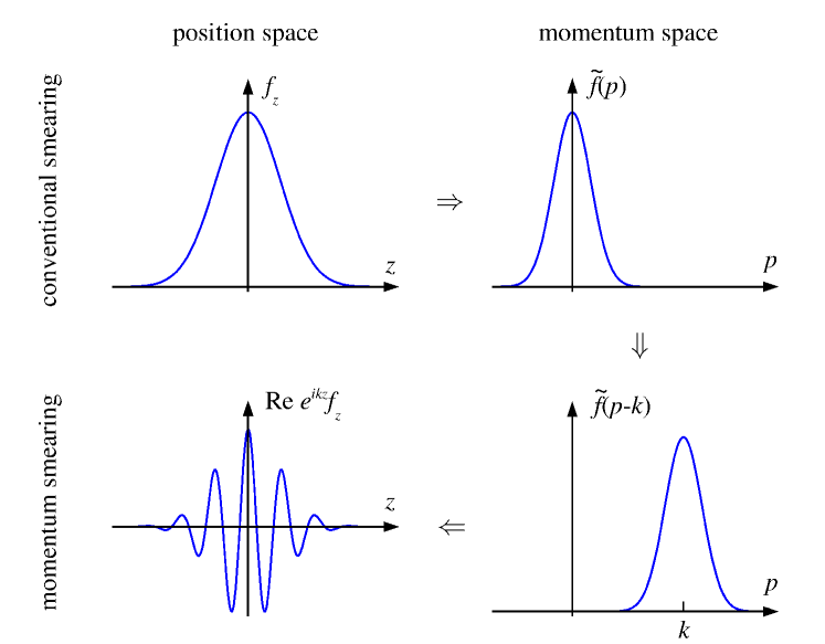
Figure 15: Conventional smearing (left) versus momentum smearing (right) Bali et al. (2016): Conventional smearing has small overlap with high momentum state. Momentum smearing shifts momentum to peak at nonzero value in momentum space.

Second, the proton size is frame-dependent and changes with its momentum. In the proton’s rest frame, simulating its structure requires that the lattice spacing be much smaller than the QCD confinement scale, i.e. $a\ll\Lambda_{\rm QCD}^{-1}$. When the proton is moving fast, it undergoes Lorentz contraction by a boost factor $\gamma$ in the momentum direction, thus a finer lattice spacing $a\ll(\gamma\Lambda_{\rm QCD})^{-1}$ is needed. If $a\leq 0.2$ fm is the minimum requirement to investigate a static proton, one will need at least $a\leq 0.04$ fm to have the same resolution for a proton at 5 GeV. A smaller lattice spacing is difficult to achieve with current computing resources, for it suffers from the well-known critical slowing down problem, i.e., the auto-correlation times of observables such as the topological charge increase when approaching the continuum limit Schaefer et al. (2011), which can be much longer than the Monte-Carlo simulation times. A lattice with open (Neumann) boundary condition on gauge fields in the Euclidean time direction Luscher and Schaefer (2011), which allows topological charge to flow in and out at boundaries of time, may overcome this problem.

Third, the gaps between the ground state and the excited state energies become smaller because of the time dilation effect. In the proton’s rest frame, the excited state contamination exponentially decays with the mass gap $\Delta M$ and evolution time $\tau$ in the form of $e^{-\Delta M\tau}$. In the boosted frame, the mass gap $\Delta M$ in the decay factor is replaced by the energy gap $\Delta E\sim\Delta M/\gamma$, and the decay changes like $e^{-\Delta M\tau}\to e^{-\Delta E\tau}=e^{-\Delta M\tau/\gamma}$ under Euclidean time evolution. Therefore, with a boosted state, a longer time evolution (source-sink separation) is needed. For example, if a source-sink separation of 1 fm is needed to separate the excited state of proton with 2 GeV momentum, a proton with 5 GeV momentum will require a source-sink separation of 2.5 fm. Even if the two-state fit technique is used, a longer time evolution is still required so that only the ground and first excited states dominate.

Last but not the least, lattice calculation requires $P^{z}\ll 1/a$, so that discretization effects of ${\cal O}((aP^{z})^{n})$ are under control. Therefore, one has to go to smaller lattice spacing in order to reach larger momentum. The quantification of ${\cal O}((aP^{z})^{n})$ effects alone in LaMET calculations has not been done, as all discretization errors are treated on equal footing in continuum extrapolation.

To summarize, to achieve a precision calculation of boosted hadron structure on lattice, a fine lattice spacing (at least in the longitudinal direction) and a large box size in the time direction are essential, which of course will also require control over the signal-to-noise ratio at large Euclidean times.

VI.1.2 Considerations for lattice setup

In practical calculations, a correlation function is first obtained on lattice in coordinate space, and then Fourier transformed to momentum space with the phase factor $e^{i\lambda x}$ where $\lambda=zP^{z}$. Therefore, the smallest $x$ one can reach can be roughly estimated from the largest $\lambda$ as $x\sim 1/\lambda$. However, a more stringent constraint comes from requiring that the higher-twist contribution ${\cal O}(\Lambda_{\rm QCD}^{2}/(xP^{z})^{2})$ be small so that the factorization is still valid, which implies $x\gg\Lambda_{\rm QCD}/P^{z}$. This also provides a rough estimate for the largest attainable $x$ ($x\ll 1-\Lambda_{\rm QCD}/P^{z}$) since the momentum fraction carried by other partons is $\sim(1-x)$ which should also be bounded from below by the above estimate.

For the current state-of-the-art simulations, the lattice spacing can reach 0.04 fm Fan et al. (2020a); Gao et al. (2020), which implies $P^{z}_{\rm max}\sim 5$ GeV and the effective resolution in longitudinal direction is about $\gamma a\sim 0.2$ fm. Thus the valid $x$ region that can be extracted from lattice is roughly 0.1 to 0.9. On the other hand, to avoid finite volume effects, it is believed that $m_{\pi}L\gtrsim 4$. For physical pion mass, the box size in spatial direction $L$ should be at least 6 fm, which means the box size is 150 lattice spacing. So far, the largest box size in LaMET calculations is 5.8 fm Lin et al. (2018a). As discussed in Sec. VI.1.1, the source-sink separation of 2.5 fm is needed for $P^{z}=5$ GeV. So the box size in time direction $T$ does not need to be particularly longer than $L$, and $T=L$ is sufficient in this lattice setup. In summary, with $a=0.04$ fm at physical pion mass, one need a $L^{3}\times T=150^{3}\times 150$ lattice to reliably extract $0.1<x<0.9$ region, which could be possible in an exa-scale computer.

There are potential tricks to reduce the computational cost. First, the required source-sink separation can be shorter if one uses a multi-state instead of two-state fit with enough statistics. However, since the number of fitting parameters in $n$-state fit grows as $n^{2}$, such a fitting will become infeasible for too large $n$. Second, note that the resolution required for transverse proton structures is not affected by the Lorentz boost, one may use a coarse lattice in the transverse directions, $a_{\perp}=0.1$ fm. The required box size is then $L_{\parallel}\times L_{\perp}^{2}\times T=150\times 60^{2}\times 150$. This asymmetric lattice can greatly reduce the resources needed for large momentum since the transverse box size is fixed. However, generating configurations and renormalization on such a lattice might bring new problems and should be further studied.

In the near future, exascale supercomputers may help to reach higher momentum, as large as 5 GeV for the proton, and improve the precision of LaMET calculations. Further theoretical developments and new ideas on the technique and algorithms are also needed to overcome the simulation difficulties.

VI.2 Non-Singlet PDFs

In this subsection, we review current status of lattice calculations of flavor non-singlet (isovector) PDFs in the proton and pion. The non-singlet case has the advantage that the mixing with gluons as well as the lattice calculation of disconnected diagrams can be avoided, thus greatly reducing the computational challenge. It is the most extensively studied parton observable with LaMET so far.

VI.2.1 Proton

The pioneering lattice studies for the isovector quark PDF in the proton were carried out in Lin et al. (2015); Alexandrou et al. (2015). These are proof-of-principle studies as the renormalization of quasi-PDFs was not well understood at that time. Nevertheless, their results encouraged the follow-up theoretical works on LaMET, including a proper renormalization and matching suitable for lattice implementations.

Certain lattice artifacts have also been studied. For example, although there is no power-divergent mixing for the quasi-PDF operators on the lattice, additional operator mixings that are not seen in the continuum can still occur if a non-chiral lattice fermion such as the Wilson-type fermion is used. In Constantinou and Panagopoulos (2017); Chen et al. (2019a) it was shown that at ${\cal O}(a^{0})$ the operator for the unpolarized quark quasi-PDF, $O_{\gamma^{z}}(z)$, can mix with the scalar operator $O_{\bf 1}(z)$, whereas $O_{\gamma^{t}}(z)$ does not. To reduce the systematic uncertainty from such mixing, $\Gamma=\gamma^{t}$ has been used since then for lattice calculations of the unpolarized quark PDF, e.g. in Alexandrou et al. (2017b); Green et al. (2018); Chen et al. (2018). Similarly, for helicity and transversity cases, one should choose $\Gamma=\gamma^{5}\gamma^{z}$ and $\Gamma=i\sigma^{z\perp}=\gamma^{\perp}\gamma^{z}$, respectively, in order to avoid the mixing. It should be noted that at ${\cal O}(a)$ all $\tilde{O}_{\Gamma}(z)$’s can mix with others Chen et al. (2019a). Nevertheless, a fine lattice spacing can reduce these effects.

In Alexandrou et al. (2017b); Chen et al. (2018); Green et al. (2018), the nonperturbative renormalization (NPR) of the quasi-PDFs was studied in the RI/MOM scheme Martinelli et al. (1995). This scheme has several advantages: The lattice regularization scheme can be converted to $\overline{\rm MS}$ scheme through RI/MOM renormalization condition, the computation cost is affordable, the systematic errors can be reduced or quantified more easily, etc. The works before 2018 did not include NPR and the systematics were not accurately quantified. The later works have implemented the RI/MOM scheme and the corresponding perturbative matching Constantinou and Panagopoulos (2017); Stewart and Zhao (2018); Liu et al. (2020). The coordinate-space method is also developed in parallel in Orginos et al. (2017); Cichy et al. (2019); Joó et al. (2019a, 2020); Bhat et al. (2020). In Figs. 16 and 17, we select some most recent lattice results. ETMC published the proton unpolarized, helicity and transversity PDFs with $P^{z}=1.4$ GeV at physical pion mass Alexandrou et al. (2018a, b), and ${\rm LP}^{3}$ published the proton helicity PDF with unprecedented momentum $P^{z}=3.0$ GeV at physical pion mass Lin et al. (2018a). Recently, calculations on fine lattices Fan et al. (2020a); Alexandrou et al. (2020c) and an extrapolation to the continuum limit Alexandrou et al. (2020c) have become available. The finite volume effects, which was first studied in a model Briceño et al. (2018), have also been investigated on the lattice lately in Lin and Zhang (2019), where no sizeable volume-dependence was observed at $P^{z}=1.3$ and $2.6$ GeV.

The PDFs extracted from LaMET can be useful for phenomenology by providing input in kinematic regions that are difficult to measure in experiments. It has attracted attention from global fit community Lin et al. (2018c); Hobbs et al. (2019); Constantinou et al. (2020); Bringewatt et al. (2020). For example, it has been found that in the large-$x$ region of unpolarized PDF the lattice result will lead to significant improvement on global fit result if it reaches an accuracy of about $10\%$ Lin et al. (2018c). The sea quark asymmetry Geesaman and Reimer (2019) is also possible to be investigated now directly on lattice. For the transversity PDF, due to the difficulty of measurement in experiment, lattice results can already have impact on improving global fit and even making predictions. In addition to the isovector cases, calculations of the strange and charm unpolarized distributions Zhang et al. (2020c), as well as the flavor separation of light quarks in the helicity PDF Alexandrou et al. (2020a), have also been carried out recently. From early exploratory results showing qualitative behavior of PDFs to the latest results which are comparable with global fits, it has come a long way in developing new techniques (momentum smearing, renormalization, matching, etc.) and the computation resources have been steadily increased over time. The systematic uncertainties in the lattice calculation of PDFs have been thorougly investigated by the ETMC Alexandrou et al. (2019b). Further studies on systematics such as the discretization effects and finite volume effects on various lattice ensembles are still necessary. In the future, lattice QCD is expected to make a significant impact on nuclon structure.

To conclude this subsection, we would like to mention that there are also lattice studies of the isovector PDF of other baryons, $\Delta^{+}$ to be more concrete, using LaMET Chai et al. (2020).

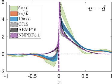
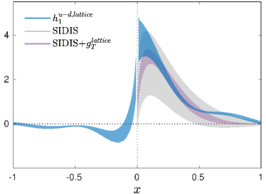
Figure 16: Proton isovector quark PDF Alexandrou et al. (2018a, b): The unpolarized PDF with $P^{z}$ from 0.82 to 1.4 GeV and the transversity PDF with $P^{z}=1.4$ GeV are in upper and lower figures. CJ15 Accardi et al. (2016a), ABMP16 Alekhin et al. (2017), and NNPDF3.1 Ball et al. (2017) are global fits. SIDIS is global fit and SIDIS$+g_{T}^{lattice}$ is global fit with lattice constraint on tensor charge $g_{T}^{lattice}$ Lin et al. (2018b).

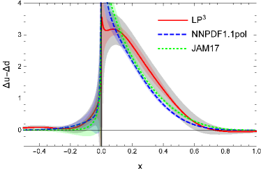
Figure 17: The proton isovector quark helicity PDF ($P^{z}=3.0$ GeV) Lin et al. (2018a) with red band for statistic error and grey band for statistic and systematic errors. NNPDF1.1pol Nocera et al. (2014) and JAM17 Ethier et al. (2017) are global fits.

VI.2.2 Pion

The pion valence quark distribution has been extracted from various Drell-Yan data for pion-nucleon/pion-nucleus scattering, while theoretical predictions do not yield consistent results with the experimental extraction, especially in large-$x$ region Holt and Roberts (2010). LaMET calculations will be able to shed valuable light on how to resolve this disagreement, provided that all systematics are well under control.

In principle, calculating the pion valence PDF is easier than the proton PDF. First, the pion state is easier to produce and the quark contractions are fewer. Second, the energy gap between the first excited and ground state of the pion is much bigger than the energy gap of the proton. Therefore, the excited-state contamination is easier to control. The simulation was first performed in Zhang et al. (2019a) with the same lattice setup and procedure used in exploratory studies of the proton PDF. A more thorough study on the pion valence quark PDF was done by the lattice QCD group of BNL Izubuchi et al. (2019). It is worth pointing out that the excited state contamination was thoroughly studied using multi-state fits, with the ground and first excited states both agreeing with the expected dispersion relations, indicating that the excited contamination is well under control. The comparison of the lattice results from quasi-PDF, pseudo-PDF and current-current correlator approach are shown in Fig. 18. Note that the $\rm LP^{3}$ Zhang et al. (2019a) result was obtained using Fourier transformation and inversion of factorization formula, while other three groups used parameterization models to fit the lattice data. More dedicated effort is needed to reduce the errors, and a meaningful comparison between different operators and analysis methods should be made.

For other mesons, we would like to mention that there is a study of kaon valence quark PDF using MILC configurations Lin et al. (2020).

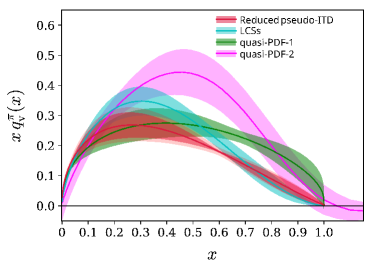
Figure 18: Pion valence quark PDFs in various approach: Compare the results of pesudo-PDF [Reduced pseudo-ITD Joó et al. (2019b)], quasi-PDF [quasi-PDF-1 Izubuchi et al. (2019) and quasi-PDF-2 Zhang et al. (2019a)], and the current-current correlator approach [LCSs Sufian et al. (2019)].

VI.3 Gluon Helicity and Other Collinear Parton Properties

In this subsection, we summarize the applications of LaMET to other collinear parton observables, including the gluon helicity, the gluon PDFs, meson DAs and GPDs.

VI.3.1 Total gluon helicity

The total gluon helicity $\Delta G$ is a key component in understanding the proton spin structure. It has been intensively explored at RHIC and will be dedicatedly pursued at EIC in the future. However, a theoretical lattice calculation of $\Delta G$ had not been possible until the proposal of LaMET.

The first such effort was made by $\chi$QCD collaboration in Yang et al. (2017). The calculation was carried out with valence overlap fermions on $2+1$ flavor domain-wall fermion gauge configurations, using ensembles with multiple lattice spacings and volumes including one with physical pion mass. The authors simulated proton matrix elements of the free-field operator $(\vec{E}\times\vec{A})^{3}$ in the Coulomb gauge at various momenta, and then converted them to the $\overline{\rm MS}$ scheme with one-loop lattice perturbation theory. The $\overline{\rm MS}$ matrix elements at each lattice momentum are shown in Fig. 19. Though a LaMET matching is necessary to match the results to the physical gluon helicity, the authors did not apply it due to the concern of perturbative convergence of the matching coefficient Ji et al. (2015c). Instead, as the $\overline{\rm MS}$ matrix elements show rather mild momentum dependence up to the maximum momentum $\sim$1.5 GeV, they extrapolated the results to infinite momentum, as well as physical pion mass and continuum limits, with a model motivated by chiral EFT. Their final result is $\Delta G(\mu^{2}=10\ \text{GeV}^{2})=0.251(47)(16)$, or 50(9)(3)% of the total proton spin, which agrees with the truncated moment of $\Delta g(x)$ de Florian et al. (2014); Nocera et al. (2014) within uncertainties.

Despite such progress, one should be cautious that this calculation still needs further improvements in the future. Among others, the most important ones are simulations at larger proton momentum, performing an NPR and investigating perturbative convergence of LaMET matching and its implementation.

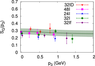
Figure 19: Total gluon helicity Yang et al. (2017): The results are extrapolated to the physical pion mass and continuum as a function of the proton momentum $p_{3}$ on all the five ensembles indicated by different colors of the data points.

VI.3.2 Gluon PDF

The gluon PDF is of great interest not only for precision physics at LHC, but also for understanding the gluonic structure of the proton and nuclei—as well as the small-$x$ dynamics—at the future EIC. With the recent progress on the renormalization and matching for gluon quasi-PDFs Wang and Zhao (2018); Wang et al. (2018); Zhang et al. (2019b); Li et al. (2019); Wang et al. (2019b) or the coordinate-space “pseudo distributions” Balitsky et al. (2019), a systematic lattice calculation of the gluon PDFs can be carried out in principle.

Before the above theoretical developments, an exploratory lattice study of the proton and pion unpolarized gluon PDFs were carried out in Fan et al. (2018). The authors calculated quasi gluon LF correlations and compared them to the LF correlations for the gluon PDFs. Later on, based on the multiplicative renormalizability of certain choice of the quasi gluon LF correlator Zhang et al. (2019b), the same authors used the ratio scheme Balitsky et al. (2019) in coordinate space to renormalize the lattice matrix elements, and fitted the proton unpolarized gluon PDF with a simple two-parameter model  Fan et al. (2020b). Although the results show agreement with the global analyses in the large-$x$ region, the systematics from the model-dependence of the fit remains to be quantified for a controlled calculation of the gluon PDF.

VI.3.3 DA

According to Sec. IV.2, LaMET can be readily applied to calculating DAs, and the lattice resource needed is expected to be cheaper than that for PDFs since there is one less external state, which reduces the number of contractions for the quark propagators. So far there are a few exploratory investigations on meson DAs, in particular, on pion Zhang et al. (2017) and kaon DAs Zhang et al. (2019c). The lattice calculations of pion Zhang et al. (2017) and kaon DAs Zhang et al. (2019c) were first explored without the NPR and the corresponding matching. Recently, the pion and kaon DAs from the RI/MOM scheme analysis are extrapolated to the continuum limit Zhang et al. (2020b), where the authors eventually adopted a two-parameter model to fit the final result. The above results are shown in Fig. 20. Apart from LaMET, the current-current correlation methods Braun and Müller (2008); Braun et al. (2015); Detmold and Lin (2006) have also made much progress on the pion DA Bali et al. (2019); Detmold et al. (2018, 2020).

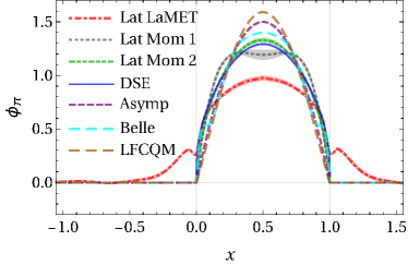
Figure 20: Pion DA Zhang et al. (2019c): Comparison of $\phi_{\pi}$ (Lat LaMET) to previous determinations in the literature. Lat Mom 1 and 2 are parameterized fits to the lattice moments Braun et al. (2015); DSE is Dyson-Schwinger equation calculations Chang et al. (2013); Asymp is the asymptotic form $6x(1-x)$; Belle is a fit to the Belle data Agaev et al. (2012); LFCQM is light-front constituent quark model de Melo et al. (2016).

VI.3.4 GPD

As discussed in Sec. IV, the global fitting of GPDs still faces challenges from their complicated kinematic dependence and limited information from the experimental observables despite the progress made Kumericki et al. (2016); Favart et al. (2016). On the other hand, previous lattice QCD method is only able to calculate the lowest few moments of the GPDs Hagler (2010), which is far from sufficient to reconstruct their full kinematic dependence. Applying LaMET to GPD calculations will provide important information on the GPDs, especially in kinematic regions that are not accessible in currently available experiments. In addition, on the lattice one can study the GPD dependence on one kinematic variable by fixing the others. All these will help differentiate commonly used models in GPD parameterization.

Calculating the quasi-GPDs requires more resources than quasi-PDF, but does not need further techniques in principle. Besides, the lattice renormalization factors for the quasi-PDFs can be used here, as has been argued in Sec. IV. The first lattice calculation of the pion unpolarized isovector quark GPD was carried out in Chen et al. (2019b), though the results are not yet able to differentiate models or compare to experiments. Recently, ETMC completed the first proof-of-principle calculation of the proton unpolarized and helicity GPDs Alexandrou et al. (2020d), as shown in Fig. 21, which demonstrates that it is feasible to extract the GPDs with controlled systematics on available computational resources.

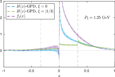
Figure 21: Proton unpolarized isovector quark GPD Alexandrou et al. (2020d) $H(x,\xi,t)$ for $t=-0.69\ {\rm GeV^{2}}$ extracted from quasi-GPDs at $P_{3}=1.25$ GeV, which is compared to the unpolarized PDF $f_{1}(x)$.

VI.3.5 Higher-twist PDF

The higher-twist PDFs probe multi-parton correlations, and their contribution at $x=0$ can shed light on the LF zero modes Ji (2020). As we discussed in Sec. IV, such distributions can also be calculated on the lattice with the LaMET approach.

The first attempt to calculate the isovector twist-three PDF $g_{T}(x)$ has been carried out by ETMC Bhattacharya et al. (2020a) using the one-loop matching coefficient they computed in Bhattacharya et al. (2020b, c). Their results show agreement with the Wandzura-Wilczeck approximation Wandzura and Wilczek (1977), which ignores the contribution from dynamical twist-three contributions, and the Burkhardt-Cottingham sum rule Burkhardt and Cottingham (1970). Nevertheless, the mixing between $g_{T}(x)$ and other twist-three distributions was not considered, and further study is still required for an accurate matching to the light-cone PDF.

VI.4 TMDs

With tremendous experimental focus on the TMDPDFs for studying 3D proton structures and gluon saturation at EIC, their first-principle calculation from lattice QCD will significantly boost this direction by providing useful nonperturbative inputs for all the phenomenological analyses.

In this subsection, we discuss the status and prospects of calculating the quasi-TMDPDF and soft function with LaMET. Besides, we note that before LaMET there had already been efforts to extract information of TMDs by studying ratios of the lattice correlators Hagler et al. (2009); Musch et al. (2011, 2012); Engelhardt et al. (2016); Yoon et al. (2017), which has made a series of progress in the past decade. We begin with a brief review of them.

VI.4.1 Pre-LaMET study — ratio of lattice correlators

By employing Lorentz covariance, the $x$-moments of TMDPDFs are related to the form factors of spacelike staple-shaped gauge link operators, which can be directly simulated on the lattice. Although the lattice calculation of the soft function was not available during that time, ratios of the spin-dependent and the unpolarized matrix elements were formed to cancel it, thus providing useful information of different TMDPDFs. For example, the time-reversal odd TMDPDFs can be studied with the staple-shaped gauge link operator in a transversely polarized proton state, thus helping understand properties related to single-spin asymmetry (SSA), which was measured experimentally at STAR Adamczyk et al. (2016) and COMPASS Aghasyan et al. (2017). In Musch et al. (2012); Engelhardt et al. (2016), the Sivers and Boer-Mulders functions of proton and pion were studied; Other time-reversal even functions, such as the worm-gear function $g_{1T}$ Tangerman and Mulders (1995), were also studied Yoon et al. (2017).

VI.4.2 Quasi-TMDPDF and Collins-Soper kernel

The lattice calculation of the quasi-TMDPDF defined in Eq. (205) is straightforward. The matrix element of the staple-shaped quark Wilson line operator can be simulated the same way as the quasi-PDF case, except that the geometry of the gauge-link is different, while the calculation of Wilson loop $Z_{E}$ is standard practice in lattice QCD. The more challenging part, however, is the renormalization of the quasi-TMDPDF and its matching to the $\overline{\rm MS}$ scheme.

Using the auxiliary field theory formalism, one can argue that staple-shaped quark Wilson line operator is also multiplicatively renormalizable Ebert et al. (2020b); Green et al. (2020). On a non-chiral lattice, it suffers from finite mixing with other quark bilinear operators, as was predicted by one-loop lattice perturbation theory Constantinou et al. (2019). The full mixing pattern for such operators with different Dirac matrices have been studied in the RI/MOM scheme on three quenched lattice ensembles with different spacings Shanahan et al. (2019), and a diagonalization of the mixing matrix is adopted to renormalize these operators. Meanwhile, the one-loop conversion factors that convert the RI/MOM matrix elements to the $\overline{\rm MS}$ scheme have been calculated in continuum perturbation theory for both the $z=0$ Constantinou et al. (2019) and $z\neq 0$ Ebert et al. (2020b) cases.

Although the soft function is still needed to fully determine the physical TMDPDF, the $\overline{\rm MS}$ quasi-TMDPDF can already be used to extract the Collins-Soper kernel according to Eq. (220) Ji et al. (2015b); Ebert et al. (2019a, b). Since the Collins-Soper kernel can be defined from both the bare TMDPDF and the soft function, it is independent of the external state and can be calculated in a pion which is the least expensive on the lattice. Up to mass corrections suppressed by the momentum in Eq. (219), this calculation also allows for using an unphysical valence pion mass, as long as the sea quark masses are physical.

With the method developed in Ebert et al. (2019a), the first exploratory lattice calculation of the Collins-Soper kernel was performed in Shanahan et al. (2020) on a quenched lattice with heavy valence pion mass $m_{\pi}\sim 1.2$ GeV, and the result is shown in Fig. 22. As one can see, the lattice prediction is robust for $0.1\ {\rm fm}<b_{\perp}<0.8\ {\rm fm}$, which covers the nonperturbative region that is important for TMD evolution in global analyses. Besides, at small $b_{\perp}$, the perturbative calculation can serve as a calibration for estimating the systematic uncertainties, as there are power corrections of ${\cal O}(1/(P^{z}b_{\perp}))$ which can only be reduced with larger $P^{z}$. In Zhang et al. (2020a), the Collins-Soper kernel has also been extracted from a pion quasi-TMD DA, where the lattice renormalization was left out, and the result is in agreement with Shanahan et al. (2020) within errors for a wide range of $b_{\perp}$. With improved lattice ensembles and systematic corrections in the future, it is promising to have a precise determination of the Collins-Soper kernel for TMD phenomenology.

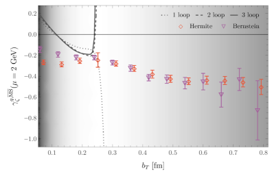
Figure 22: The Collins-Soper kernel from the first exploratory calculation on a quenched lattice Shanahan et al. (2020). The results are obtained by using fits to the ${\overline{\rm MS}}$ unsubtracted quasi-TMDPDFs with Hermite and Bernstein polynomial bases. The solid and dashed lines are the perturbative predictions Li and Zhu (2017); Vladimirov (2018), which is hit the Landau pole near $b_{\perp}\sim 0.25$ fm. The background shading density is proportional to a naive estimate of the power corrections $1/(b_{\perp}P^{z})+b_{\perp}/L$.

VI.4.3 Soft function

As the remaining piece towards physical TMDPDFs, the soft function must be calculated in lattice QCD. In particular, the reduced soft function in Eq. (214) eliminates the regulator-scheme-dependence of the off-the-light-cone quasi-TMDPDF, so its calculation alone has great physical significance. According to Secs. (V.3) and (V.4), two methods have been proposed to calculate the off-the-light-cone soft function or reduced soft function on the lattice Ji et al. (2020a), as we discuss in the following. One relies on simulating HQET on the lattice, while the other requires calculating a light-meson form factor of transversely-separated current products.

The latter method has been implemented in the first exploratory lattice calculation of the reduced soft function Zhang et al. (2020a), which includes simulations of the pion form factor in two external states with opposite large momenta, as well as the pion quasi-TMD DA. The results for the reduced soft function, which are obtained with tree-level matching and omission of lattice renormalization, are shown in Fig. 23. As one can see, they agree with the perturbative prediction for small $b_{\perp}$ within errors, as expected, and start to deviate when $b_{\perp}$ becomes large. Since the quasi-TMD DA depends on the momentum $P^{z}$, the stability of results at different $P^{z}$ suggests the validity of Eq. (260). In the future, larger statistics and improved systematics in both lattice and perturbative matching will be necessary to achieve a precision calculation of this quanity.

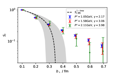
Figure 23: The reduced soft factor as a function of $b_{\perp}$ extracted from the light-meson form factor in Sec. V Zhang et al. (2020a). The results are obtained with quasi-TMD DAs at different pion momentum $P^{z}$, with perturbative matching and power corrections ignored. The dashed line is one-loop prediction in perturbation theory, which hits the Landau pole at $b_{\perp}\sim 0.3$ fm, and the grey band is the error by varying $\mu$ by a factor of $1/\sqrt{2}$ and $\sqrt{2}$.

VII Conclusion and Outlook

Since Feynman proposed the parton model more than fifty years ago, our understanding of the partonic structure of the proton has been greatly advanced. On one hand, a number of high-energy experiments carried out at facilities worldwide including SLAC, DESY, CERN, Fermi Lab, JLab, BNL, etc. allowed us to probe various aspects of hadronic structures at different energies and polarizations. On the other hand, many parton observables have been proposed in parallel that provide a multi-dimensional description of the proton structure, including the collinear PDFs, TMDPDFs, GPDs, parton DAs, LFWFs and so on.

Although QCD factorization theorems with RG improvement allow us to extract these parton observables through their connection to experimental observables, it is highly desirable to predict them from ab initio calculations such as lattice QCD. Developments along this line have been rather slow due to difficulties in simulating real-time dynamics. The situation, however, has changed since the proposal of LaMET a few years ago, which provides a systematically improvable method to calculate parton physics from first principles.

In this paper, we give an overview of LaMET formalism and its applications to observables which can be accessed in lattice QCD and other non-perturbative methods. By investigating the frame dependence of the structure of bound state hadrons, we explain how the IMF physics or parton physics naturally arises as an EFT description of the proton structure. Such an EFT description is most naturally formulated in SCET and LFQ, but practical non-perturbative calculations of the proton matrix elements have been difficult. LaMET in effect provides what is needed to realize LFQ. This is achieved by forming appropriate quasi parton observables in a large momentum state and match them to the true parton observables on the LF through factorization. In the case of PDFs, the former corresponds to finite-momentum distributions whose running is controlled by the momentum RGE, whereas the latter corresponds to IMF PDFs whose running is controlled by the usual RGE. It should be pointed out that LaMET is a very general framework which can be applied to large-momentum physical quantities calculated with any non-perturbative methods, either Euclidean (with imaginary time) or Minkowskian (with real time). Moreover, given a large momentum state, the same parton physics can be determined from different quasi observables that form a universality class.

We then present how to calculate the parton observables in practice, with a particular focus on the collinear PDFs, GPDs, DAs, TMDPDFs and LFWFs. We also discuss the proton spin structure and show how the partonic contributions to proton spin can be obtained following the same approach. We finally summarize the lattice studies carried out so far with LaMET which, on one hand, demonstrate that LaMET is a promising approach to compute partonic structures of the proton, and on the other hand, clearly indicate that a lot of improvements are still required to reach such an accuracy that the lattice results can have considerable impact on phenomenology.

We complete this review with a few comments on improvements of lattice calculations for the future. We recommend Alexandrou et al. (2019b) for more systematic discussion on some of the issues, for example, the continuum, infinite volume, and physical pion mass limits.

• Large hadron momentum. Since the future of LaMET lies in larger momenta which naturally require smaller lattice spacings, it will be critical to address the challenges from using large momenta and small spacings for exa-scale computations, such as the excited state contamination or topological charge freezing problem.

• Renormalization. As discussed in Sec. III.4, the mass renormalization of Wilson line operators is favored for it is gauge invariant and does not introduce extra higher-twist effects or large statistical errors at long distance. However, its matching to the ${\overline{\rm MS}}$ scheme, especially the renormalon ambiguities, still needs to be resolved for a full systematic application. Moreover, alternative schemes that include the above features are also highly desirable.

• Higher-order perturbative matching. In current LaMET calculations, one-loop perturbative matching has brought considerable corrections. Higher-order matching kernels will be necessary to control the systematics from this procedure.

• Power corrections. They are important if the hadron momentum is not very large or when $x$ is close to 0 or 1. Little progress has been made toward a model-independent determination of the power corrections so far. One contingent strategy is to extrapolate to $P^{z}\to\infty$ limit after implementing matching and target-mass corrections, but the ultimate solution relies on the lattice calculation of higher-twist distributions that has been discussed in Sec. IV.3.

The above discussion of systematics is generic and applies to all quasi-observables. The rich theoretical developments in the past years have paved the way for calculating a wide range of parton observables using LaMET. With the rapid increase in computing resources and progress in developing new techniques and algorithms, we expect to see the above systematics to be kept under control step by step in the future. That would be important in establishing LaMET as a systematic approach to computing parton physics, and making lattice calculations play a crucial role in the EIC era.

Appendix A: Acronyms, abbreviations and terminologies

Here we list some acronyms, abbreviations and terminologies used throughout this review:

$$\begin{array}[]{L@{\qquad}L}AM&angular momentum\\ BFKL&Balitsky\textendash Fadin\textendash Kuraev\textendash Lipatov\\ BPHZ&Bogoliubov-Parasiuk-Hepp-Zimmermann\\ BRST&Becchi-Rouet-Stora-Tyutin\\ DA&distribution amplitude\\ DGLAP&Dokshizer-Gribov-Lipatov-Altarelli-Parisi\\ DIS&deep-inelastic scattering\\ DR&dimensional regularization\\ DVCS&deeply-virtual Compton scattering\\ DVMP&deeply-virtual meson production\\ DY&Drell-Yan\\ EFT&effective field theory\\ EIC&Electron-Ion Collider\\ EOM&equation of motion\\ ERBL&Efremov-Radyushkin-Brodsky-Lepage\\ GCPO&generalized collinear parton observable\\ GPD&generalized parton distribution\\ GTMD&generalized transverse-momentum-\\ &dependent distribution\\ HQET&heavy-quark effective theory\\ IMF&infinite-momentum frame\\ IR&infrared\\ LaMET&large momentum effective theory\\ LC&light-cone\\ LF&light-front\\ LFWF&light-front wave function\\ $\overline{\rm MS}$&modified minimal subtraction\\ NPR&non-perturbative renormalization\\ OAM&orbital angular momentum\\ OPE&operator product expansion\\ PDF&parton distribution function\\ QCD&quantum chromodynamics\\ QED&quantum electrodynamics\\ QFT&quantum field theory\\ RGE&renormalization group equation\\ RI/MOM&regularization-independent\\ &momentum subtraction\\ SCET&soft-collinear effective theory\\ SIDIS&semi-inclusive deep-inelastic scattering\\ TMD&transverse-momentum-dependent\\ UV&ultraviolet\end{array}$$

• Parton model: a model proposed by R. Feynman in which hadrons are viewed as a collection of point-like quasi-free partons.

• Parton distribution function: a probability function describing how the longitudinal momentum is distributed among the partons (quarks and gluons) in a hadron.

• Factorization theorem: a theorem that separates hadronic observables into process-dependent short-distance partonic observables and universal long-distance functions characterizing the hadron structure.

• Light-front quantization: a quantization program that is carried out at equal light-front time and yields a relativistic description of QCD bound states in terms of light-front wave functions.

• Bjorken $x_{B}$: The variable proposed by J. D. Bjorken to characterize the kinematics in DIS. Its definition is given above Eq. (I.1).

• Scaling: The behavior that an observable is independent of the scale at which it is probed.

• Effective field theory: a theory framework that describes physical phenomena at a given length scale using only active degrees of freedom at that scale, while integrating out degrees of freedom at other length scales.

• Renormalization group equation: an equation that describes how a physical system can be viewed and interpreted at different scales.

• HQET: an effective field theory obtained from QCD by taking the infinite heavy quark mass limit.

• Gauge link or Wilson line: a nonlocal quantity constructed as exponentials of integrals of gauge fields along a given path, used to connect fields at different spacetime points to maintain gauge invariance.

• Compton amplitude: the quantum amplitude for scattering of a (virtual) photon by the proton.

• Auxiliary field approach: an approach in which the nonlocal gauge link can be replaced by the two-point function of the auxiliary field.

• Matching: a procedure used to relate full theory operators to effective field theory operators.

• Nonsinglet: a combination accounting for the difference between quark distributions, e.g., the isovector combination $u-d$ discussed extensively in the context of this review.

• Universality class: a collection of operators that flow into the same fixed point under momentum renormalization group running.

• Quasi-light-front correlations: spatial correlations defining the finite momentum distributions.

• Collinear divergence: divergence in a Feynman diagram when loop momentum of the internal line is collinear to that of the external massless particle.

• Two-particle-irreducible diagram: a Feynman diagram that cannot be divided into disconnected parts by cutting two internal lines.

• Wilson fermion: a way to discretize the QCD fermion action on the lattice, which breaks down the chiral symmetry.

• Generalized parton distribution: generalization of PDFs to non-forward kinematics, i.e., the initial and final states have different momenta.

• Skewness: defined to characterize the longitudinal momentum transfer in GPDs.

• Distribution amplitude: transition matrix element between vacuum and hadron state, representing the probability amplitude of finding a given Fock state in the hadron.

• Twist: defined as dimension - spin of the operator. Leading-twist (higher-twist) denotes the leading (nonleading) power behavior in the quantity under investigation.

• Zero-mode: the degrees of freedom with zero longitudinal momentum in LFQ.

• Transverse momentum dependent(TMD) PDF: defined in Eq. (230), the distribution function of both longitudinal and transverse momentum for partons.

• Staple-shaped gauge-link: the pair of gauge-links separated along transverse directions that appear in the definition of TMD-PDFs, they are defined in Eq. (176), Eq. (183) and Eq. (206).

• Rapidity divergence: the divergence of TMDPDF and soft functions due to the presence of infinite rapidity scale introduced by the infinite-long gauge-links.

• Light-cone regulator: regulators that regulates the rapidity divergence. First appeared in the paragraph of Eq. (178).

• On-light-cone: rapidity regulator that maintain the presence of light-like separations in the gauge-link.

• Off-light-cone: rapidity regulator that makes the separations of the gauge-link non-light-like.

• Soft function: functions that capture the factorable soft radiations of TMDPDF. Defined in Eq. (V.1) for on-light-cone and Eq. (212) for off-light-cone.

• Collins Soper kernel: the kernel for rapidity evolution of TMDPDF, see Eq. (201).

• Quasi-TMDPDF: defined in Eq. (205), similar to TMDPDF but with light-like separations replaced by space-like ones.

• Pinch-pole singularity: the divergence due to infinite long gauge-link pair in the quasi-TMDPDF. Can be subtracted out by the factor $Z_{E}$, see discussion below Eq. (208).

• Off-light-cone soft function: soft function using off-light-cone regulator. Defined in Eq. (212) and Eq. (V.3). Required for matching quasi-TMDPDF to TMDPDF.

• Reduced soft function: the rapidity independent part of off-light-cone soft function, see Eq. (214).

• Light-Front wave function: the wave function for hadron state in light-front quantization, expanded in the Free -Fock state.

• Reduced diagram: the diagram showing the power-leading region of IR divergences. All the IR safe propagators are shrunk to blobs.

• Momentum smearing: a lattice technique to increase the overlap of the field and nonzero-momentum state.

• Non-singlet: transforms under the fundmental representation of $SU(N_{f})$ with $N_{f}$ the quark flavor number.

Appendix B: Conventions

We use the following convention for the metric tensor

$$g^{\mu\nu}=\text{diag}\,(1,-1,-1,-1)\,.$$ (263)

In ordinary coordinates, a generic four-vector is denoted as $v^{\mu}=(v^{0},v^{x},v^{y},v^{z})$ or $v^{\mu}=(v^{0},{\vec{v}}_{\perp},v^{z})$. For example, the spacelike and timelike direction vector are written as $n_{z}=(0,0,0,1)$ and $n_{t}=(1,0,0,0)$, respectively. In light-cone coordinates $\xi^{\pm}={1\over\sqrt{2}}(\xi^{0}\pm\xi^{3})$, a vector is denoted as $v^{\mu}=(v^{+},v^{-},{\vec{v}}_{\perp})$.

The hadron state $|P\rangle$ is normalized as

$$\langle P^{\prime}|P\rangle=(2\pi)^{3}2P^{0}\delta^{(3)}(\vec{P}-\vec{P}^{\prime})\,.$$ (264)

The covariant derivative and the Wilson line gauge link in the fundamental representation are defined as

$$D^{\mu}\psi=(\partial^{\mu}+igA^{\mu})\psi=(\partial^{\mu}+igt^{a}A_{a}^{\mu})\psi,$$ (265)

and

$$W(x_{2},x_{1})=$$

$$\exp\left[-ig\int_{0}^{1}dt(x_{2}-x_{1})_{\mu}A^{\mu}(x_{1}+(x_{2}-x_{1})t)\right]\,.$$ (266)

The ones in the adjoint representation are completely analogous.

We use $O_{\Gamma}(s)$ to generically denote an operator defining the corresponding (quasi) parton observable, where $s$ can be a lightlike (for parton observables) or spacelike (for quasi parton observables) separation, and $\Gamma$ is a Dirac structure. The momentum fraction in a quasi-observable is denoted as $y$, while that in the usual parton observable is denoted as $x$.

The lightcone operator that defines the quark parton observable is

$$O_{\Gamma}(\lambda n)=\bar{\psi}(0)\Gamma W(0,\lambda n)\psi(\lambda n)$$ (267)

with $\Gamma$ denoting a Dirac matrix. If we take $\Gamma=\not{n}\equiv\gamma^{+}$, the unpolarized quark PDF is then given by

$$q(x)=\frac{1}{2P^{+}}\int\frac{d\lambda}{2\pi}e^{ix\lambda}\langle P|O_{\gamma^{+}}(\lambda n)|P\rangle$$ (268)

with $n^{\mu}=1/\sqrt{2}(1/P^{+},0,0,-1/P^{+})$.

Accordingly, the quark quasi-observable is defined by

$${O}_{\Gamma}(z)=\bar{\psi}(zn_{z}/2)\Gamma W(zn_{z}/2,-zn_{z}/2)\psi(-zn_{z}/2)\ .$$ (269)

If we choose $\Gamma=\gamma^{t}$, the unpolarized quark quasi-PDF is then defined as

$${\tilde{q}}(y)=\frac{1}{2P^{0}}\int\frac{d\lambda}{2\pi}e^{iy\lambda}\langle P|{O}_{\gamma^{t}}(z)|P\rangle$$ (270)

with the quasi light-cone distance $\lambda=zP^{z}$.

The staple-shaped gauge link required for the TMDPDFs is defined as:

$${\cal W}_{n}(\lambda n/2+\vec{b}_{\perp})=W^{\dagger}_{n}(\lambda n/2+\vec{b}_{\perp})W_{\perp}W_{n}(-\lambda n/2)\ ,$$ (271)

where

$$W_{n}(\xi)=W(\xi+\infty n,\xi)\ .$$ (272)

The un-subtracted unpolarized quark TMDPDF is then defined as:

$$f(x,\vec{k}_{\perp},\mu,\delta^{-}/P^{+})=\frac{1}{2P^{+}}\int\frac{d\lambda}{2\pi}\frac{d^{2}\vec{b}_{\perp}}{(2\pi)^{2}}e^{-i\lambda x+i\vec{k}_{\perp}\cdot\vec{b}_{\perp}}$$

$$\times\langle P|\bar{\psi}(\lambda n/2+\vec{b}_{\perp})\not{n}{\cal W}_{n}(\lambda n/2+\vec{b}_{\perp})|_{\delta^{-}}\psi(-\lambda n/2)|P\rangle\ ,$$ (273)

and the TMD soft function for DY process is defined as:

$$S(b_{\perp},\mu,\delta^{+},\delta^{-})$$

$$=\frac{{\rm Tr}\langle 0|{\cal\bar{T}}W_{p}(\vec{b}_{\perp})|_{\delta^{+}}W_{n}^{\dagger}(\vec{b}_{\perp})|_{\delta^{-}}{\cal T}W_{n}(0)|_{\delta^{-}}W^{\dagger}_{p}(0)|_{\delta^{+}}|0\rangle}{N_{c}}$$

$$=\frac{{\rm Tr}\langle 0|{\cal W}_{n}(\vec{b}_{\perp})|_{\delta^{+}}{\cal W}^{\dagger}_{p}(\vec{b}_{\perp})|_{\delta^{-}}|0\rangle}{N_{c}}\,,$$ (274)

where $|_{\delta^{\pm}}$ denotes the rapidity regulator for the gauge links involved. In terms of these, the physical scheme independent TMDPDF is defiend as:

$$f^{\rm TMD}(x,b_{\perp},\mu,\zeta)=\lim_{\delta^{-}\rightarrow 0}\frac{f(x,b_{\perp},\mu,\delta^{-}/P^{+})}{\sqrt{S(b_{\perp},\mu,\delta^{-}e^{2y_{n}},\delta^{-})}}\ ,$$ (275)

where $\zeta\equiv 2(xP^{+})^{2}e^{2y_{n}}$ is the rapidity scale.

The staple-shaped gauge link for the quasi-TMDPDF is defined as:

$${\cal W}_{z}(\frac{\lambda n_{z}}{2}+\vec{b}_{\perp};L)=W^{\dagger}_{z}(\xi;L)W_{\perp}W_{z}(-\xi^{z}n_{z};L)\ ,$$ (276)

where

$$W_{z}(\xi)=W(\xi+(L-\xi^{z})n_{z},\xi)\ .$$ (277)

The quasi-TMDPDF is then defined using ${\cal W}_{z}(\frac{\lambda n_{z}}{2}+\vec{b}_{\perp};L)$ in exactly the same way as that for the un-subtracted TMDPDF:

$$\tilde{f}(\lambda,b_{\perp},\mu,\zeta_{z})=$$ (278)

$$\lim_{L\rightarrow\infty}\frac{\langle P|\bar{\psi}\left(\frac{\lambda n_{z}}{2}+\vec{b}_{\perp}\right)\gamma^{z}{\cal W}_{z}(\frac{\lambda n_{z}}{2}+\vec{b}_{\perp};L)\psi\left(-\frac{\lambda n_{z}}{2}\right)|P\rangle}{\sqrt{Z_{E}(2L,b_{\perp},\mu)}}\ ,$$

where $Z_{E}(2L,b_{\perp},\mu)$ is a flat rectangular Euclidean Wilson-loop along the $n_{z}$ direction with length $2L$ and width $b_{\perp}$:

$$Z_{E}(2L,b_{\perp},\mu)=\frac{1}{N_{c}}{\rm Tr}\langle 0|W_{\perp}{\cal W}_{z}(\vec{b}_{\perp};2L)|0\rangle\ .$$ (279)

The staple-shaped operators for LFWFs and quasi-LFWFs are the same as those for TMD-PDFs and quasi-TMDPDFs, and can be found in Sec. V.4.

References

- Abada et al. (2001) Abada, A, Philippe Boucaud, G. Herdoiza, J. P. Leroy, J. Micheli, O. Pene, and J. Rodriguez-Quintero (2001), “Preliminaries on a lattice analysis of the pion light cone wave function: A Partonic signal?” Phys. Rev. D64, 074511, arXiv:hep-ph/0105221 [hep-ph] .
- Abdel-Rehim et al. (2015) Abdel-Rehim, A, et al. (2015), “Nucleon and pion structure with lattice QCD simulations at physical value of the pion mass,” Phys. Rev. D92 (11), 114513, [Erratum: Phys. Rev.D93,no.3,039904(2016)], arXiv:1507.04936 [hep-lat] .
- Accardi et al. (2016a) Accardi, A, L. T. Brady, W. Melnitchouk, J. F. Owens, and N. Sato (2016a), “Constraints on large- parton distributions from new weak boson production and deep-inelastic scattering data,” Phys. Rev. D93 (11), 114017, arXiv:1602.03154 [hep-ph] .
- Accardi et al. (2016b) Accardi, A, et al. (2016b), “Electron Ion Collider: The Next QCD Frontier,” Eur. Phys. J. A52 (9), 268, arXiv:1212.1701 [nucl-ex] .
- Adamczyk et al. (2016) Adamczyk, L, et al. (STAR) (2016), “Measurement of the transverse single-spin asymmetry in at RHIC,” Phys. Rev. Lett. 116 (13), 132301, arXiv:1511.06003 [nucl-ex] .
- Agaev et al. (2012) Agaev, S S, V. M. Braun, N. Offen, and F. A. Porkert (2012), “BELLE Data on the Form Factor: A Game Changer?” Phys. Rev. D86, 077504, arXiv:1206.3968 [hep-ph] .
- Aghasyan et al. (2017) Aghasyan, M, et al. (COMPASS) (2017), “First measurement of transverse-spin-dependent azimuthal asymmetries in the Drell-Yan process,” Phys. Rev. Lett. 119 (11), 112002, arXiv:1704.00488 [hep-ex] .
- Aglietti (1994) Aglietti, U (1994), “Consistency and lattice renormalization of the effective theory for heavy quarks,” Nucl. Phys. B421, 191–216, arXiv:hep-ph/9304274 [hep-ph] .
- Aglietti et al. (1998) Aglietti, U, Marco Ciuchini, G. Corbo, E. Franco, G. Martinelli, and L. Silvestrini (1998), “Model independent determination of the light cone wave functions for exclusive processes,” Phys. Lett. B441, 371–375, arXiv:hep-ph/9806277 [hep-ph] .
- Aidala et al. (2013) Aidala, Christine A, Steven D. Bass, Delia Hasch, and Gerhard K. Mallot (2013), “The Spin Structure of the Nucleon,” Rev. Mod. Phys. 85, 655–691, arXiv:1209.2803 [hep-ph] .
- Alekhin et al. (2017) Alekhin, S, J. Blümlein, S. Moch, and R. Placakyte (2017), “Parton distribution functions, , and heavy-quark masses for LHC Run II,” Phys. Rev. D96 (1), 014011, arXiv:1701.05838 [hep-ph] .
- Alexandrou et al. (2019a) Alexandrou, C, S. Bacchio, M. Constantinou, J. Finkenrath, K. Hadjiyiannakou, K. Jansen, G. Koutsou, and A. Vaquero Aviles-Casco (2019a), “The nucleon axial, tensor and scalar charges and -terms in lattice QCD,” arXiv:1909.00485 [hep-lat] .
- Alexandrou et al. (2017a) Alexandrou, C, M. Constantinou, K. Hadjiyiannakou, K. Jansen, C. Kallidonis, G. Koutsou, A. Vaquero Avilés-Casco, and C. Wiese (2017a), “Nucleon Spin and Momentum Decomposition Using Lattice QCD Simulations,” Phys. Rev. Lett. 119 (14), 142002, arXiv:1706.02973 [hep-lat] .
- Alexandrou et al. (2020a) Alexandrou, C, M. Constantinou, K. Hadjiyiannakou, K. Jansen, and F. Manigrasso (2020a), “Flavor decomposition for the proton helicity parton distribution functions,” arXiv:2009.13061 [hep-lat] .
- Alexandrou et al. (2020b) Alexandrou, C, et al. (2020b), “Moments of nucleon generalized parton distributions from lattice QCD simulations at physical pion mass,” Phys. Rev. D101 (3), 034519, arXiv:1908.10706 [hep-lat] .
- Alexandrou et al. (2020c) Alexandrou, Constantia, Krzysztof Cichy, Martha Constantinou, Jeremy R. Green, Kyriakos Hadjiyiannakou, Karl Jansen, Floriano Manigrasso, Aurora Scapellato, and Fernanda Steffens (2020c), “Lattice continuum-limit study of nucleon quasi-PDFs,” arXiv:2011.00964 [hep-lat] .
- Alexandrou et al. (2017b) Alexandrou, Constantia, Krzysztof Cichy, Martha Constantinou, Kyriakos Hadjiyiannakou, Karl Jansen, Haralambos Panagopoulos, and Fernanda Steffens (2017b), “A complete non-perturbative renormalization prescription for quasi-PDFs,” Nucl. Phys. B923, 394–415, arXiv:1706.00265 [hep-lat] .
- Alexandrou et al. (2019b) Alexandrou, Constantia, Krzysztof Cichy, Martha Constantinou, Kyriakos Hadjiyiannakou, Karl Jansen, Aurora Scapellato, and Fernanda Steffens (2019b), “Systematic uncertainties in parton distribution functions from lattice QCD simulations at the physical point,” Phys. Rev. D99 (11), 114504, arXiv:1902.00587 [hep-lat] .
- Alexandrou et al. (2020d) Alexandrou, Constantia, Krzysztof Cichy, Martha Constantinou, Kyriakos Hadjiyiannakou, Karl Jansen, Aurora Scapellato, and Fernanda Steffens (2020d), “Unpolarized and helicity generalized parton distributions of the proton within lattice QCD,” arXiv:2008.10573 [hep-lat] .
- Alexandrou et al. (2018a) Alexandrou, Constantia, Krzysztof Cichy, Martha Constantinou, Karl Jansen, Aurora Scapellato, and Fernanda Steffens (2018a), “Light-Cone Parton Distribution Functions from Lattice QCD,” Phys. Rev. Lett. 121 (11), 112001, arXiv:1803.02685 [hep-lat] .
- Alexandrou et al. (2018b) Alexandrou, Constantia, Krzysztof Cichy, Martha Constantinou, Karl Jansen, Aurora Scapellato, and Fernanda Steffens (2018b), “Transversity parton distribution functions from lattice QCD,” Phys. Rev. D98 (9), 091503, arXiv:1807.00232 [hep-lat] .
- Alexandrou et al. (2015) Alexandrou, Constantia, Krzysztof Cichy, Vincent Drach, Elena Garcia-Ramos, Kyriakos Hadjiyiannakou, Karl Jansen, Fernanda Steffens, and Christian Wiese (2015), “Lattice calculation of parton distributions,” Phys. Rev. D92, 014502, arXiv:1504.07455 [hep-lat] .
- Altarelli and Parisi (1977) Altarelli, Guido, and G. Parisi (1977), “Asymptotic Freedom in Parton Language,” Nucl. Phys. B126, 298–318.
- Aoki et al. (2020) Aoki, S, et al. (Flavour Lattice Averaging Group) (2020), “FLAG Review 2019,” Eur. Phys. J. C80 (2), 113, arXiv:1902.08191 [hep-lat] .
- Aoki et al. (2010) Aoki, Yasumichi, Tom Blum, Huey-Wen Lin, Shigemi Ohta, Shoichi Sasaki, Robert Tweedie, James Zanotti, and Takeshi Yamazaki (2010), “Nucleon isovector structure functions in (2+1)-flavor QCD with domain wall fermions,” Phys. Rev. D82, 014501, arXiv:1003.3387 [hep-lat] .
- Aprahamian et al. (2015) Aprahamian, Ani, et al. (2015), “Reaching for the horizon: The 2015 long range plan for nuclear science,” .
- Arefeva (1980) Arefeva, IYa (1980), “QUANTUM CONTOUR FIELD EQUATIONS,” Phys. Lett. B 93, 347–353.
- Aubert et al. (2009) Aubert, Bernard, et al. (BaBar) (2009), “Measurement of the gamma gamma* —> pi0 transition form factor,” Phys. Rev. D80, 052002, arXiv:0905.4778 [hep-ex] .
- Bacchetta et al. (2019) Bacchetta, Alessandro, Valerio Bertone, Chiara Bissolotti, Giuseppe Bozzi, Filippo Delcarro, Fulvio Piacenza, and Marco Radici (2019), “Transverse-momentum-dependent parton distributions up to N3LL from Drell-Yan data,” arXiv:1912.07550 [hep-ph] .
- Bacchetta et al. (2017) Bacchetta, Alessandro, Filippo Delcarro, Cristian Pisano, Marco Radici, and Andrea Signori (2017), “Extraction of partonic transverse momentum distributions from semi-inclusive deep-inelastic scattering, Drell-Yan and Z-boson production,” JHEP 06, 081, [Erratum: JHEP06,051(2019)], arXiv:1703.10157 [hep-ph] .
- Bagan and Gosdzinsky (1994) Bagan, E, and P. Gosdzinsky (1994), “Renormalizability of the heavy quark effective theory,” Phys. Lett. B320, 123–129, arXiv:hep-ph/9305297 [hep-ph] .
- Baikov et al. (2009) Baikov, PA, K.G. Chetyrkin, A.V. Smirnov, V.A. Smirnov, and M. Steinhauser (2009), “Quark and gluon form factors to three loops,” Phys. Rev. Lett. 102, 212002, arXiv:0902.3519 [hep-ph] .
- Bali et al. (2019) Bali, Gunnar S, Vladimir M. Braun, Simon Bürger, Meinulf Göckeler, Michael Gruber, Fabian Hutzler, Piotr Korcyl, Andreas Schäfer, André Sternbeck, and Philipp Wein (2019), “Light-cone distribution amplitudes of pseudoscalar mesons from lattice QCD,” JHEP 08, 065, arXiv:1903.08038 [hep-lat] .
- Bali et al. (2018a) Bali, Gunnar S, Vladimir M. Braun, Benjamin Gläßle, Meinulf Göckeler, Michael Gruber, Fabian Hutzler, Piotr Korcyl, Andreas Schäfer, Philipp Wein, and Jian-Hui Zhang (2018a), “Pion distribution amplitude from Euclidean correlation functions: Exploring universality and higher-twist effects,” Phys. Rev. D98 (9), 094507, arXiv:1807.06671 [hep-lat] .
- Bali et al. (2014) Bali, Gunnar S, Sara Collins, Benjamin Gläßle, Meinulf Göckeler, Johannes Najjar, Rudolf H. Rödl, Andreas Schäfer, Rainer W. Schiel, André Sternbeck, and Wolfgang Söldner (2014), “The moment of the nucleon from lattice QCD down to nearly physical quark masses,” Phys. Rev. D90 (7), 074510, arXiv:1408.6850 [hep-lat] .
- Bali et al. (2016) Bali, Gunnar S, Bernhard Lang, Bernhard U. Musch, and Andreas Schäfer (2016), “Novel quark smearing for hadrons with high momenta in lattice QCD,” Phys. Rev. D93 (9), 094515, arXiv:1602.05525 [hep-lat] .
- Bali et al. (2018b) Bali, Gunnar S, et al. (2018b), “Pion distribution amplitude from Euclidean correlation functions,” Proceedings, 35th International Symposium on Lattice Field Theory (Lattice 2017): Granada, Spain, June 18-24, 2017, Eur. Phys. J. C78 (3), 217, arXiv:1709.04325 [hep-lat] .
- Balitsky (1996) Balitsky, I (1996), “Operator expansion for high-energy scattering,” Nucl. Phys. B463, 99–160, arXiv:hep-ph/9509348 [hep-ph] .
- Balitsky et al. (1996) Balitsky, I I, Vladimir M. Braun, Y. Koike, and K. Tanaka (1996), “Q**2 evolution of chiral odd twist - three distributions h(L) (x, Q**2) and e (x, Q**2) in the large N(c) limit,” Phys. Rev. Lett. 77, 3078–3081, arXiv:hep-ph/9605439 [hep-ph] .
- Balitsky and Lipatov (1978) Balitsky, I I, and L. N. Lipatov (1978), “The Pomeranchuk Singularity in Quantum Chromodynamics,” Sov. J. Nucl. Phys. 28, 822–829, [Yad. Fiz.28,1597(1978)].
- Balitsky et al. (2019) Balitsky, Ian, Wayne Morris, and Anatoly Radyushkin (2019), “Gluon Pseudo-Distributions at Short Distances: Forward Case,” arXiv:1910.13963 [hep-ph] .
- Balitsky and Braun (1989) Balitsky, II, and Vladimir M. Braun (1989), “Evolution Equations for QCD String Operators,” Nucl. Phys. B 311, 541–584.
- Ball et al. (2006) Ball, Patricia, V. M. Braun, and A. Lenz (2006), “Higher-twist distribution amplitudes of the K meson in QCD,” JHEP 05, 004, arXiv:hep-ph/0603063 [hep-ph] .
- Ball et al. (2017) Ball, Richard D, et al. (NNPDF) (2017), “Parton distributions from high-precision collider data,” Eur. Phys. J. C77 (10), 663, arXiv:1706.00428 [hep-ph] .
- Barone et al. (2002) Barone, Vincenzo, Alessandro Drago, and Philip G. Ratcliffe (2002), “Transverse polarisation of quarks in hadrons,” Phys. Rept. 359, 1–168, arXiv:hep-ph/0104283 [hep-ph] .
- Bars and Green (1978) Bars, I, and Michael B. Green (1978), “Poincare and Gauge Invariant Two-Dimensional QCD,” Phys. Rev. D17, 537.
- Bass (2005) Bass, Steven D (2005), “The Spin structure of the proton,” Rev. Mod. Phys. 77, 1257–1302, arXiv:hep-ph/0411005 .
- Bauer et al. (2001) Bauer, Christian W, Sean Fleming, Dan Pirjol, and Iain W. Stewart (2001), “An Effective field theory for collinear and soft gluons: Heavy to light decays,” Phys. Rev. D63, 114020, arXiv:hep-ph/0011336 [hep-ph] .
- Bauer et al. (2002) Bauer, Christian W, Dan Pirjol, and Iain W. Stewart (2002), “Soft collinear factorization in effective field theory,” Phys. Rev. D65, 054022, arXiv:hep-ph/0109045 [hep-ph] .
- Bauer and Stewart (2001) Bauer, Christian W, and Iain W. Stewart (2001), “Invariant operators in collinear effective theory,” Phys. Lett. B516, 134–142, arXiv:hep-ph/0107001 [hep-ph] .
- Becher and Neubert (2011) Becher, Thomas, and Matthias Neubert (2011), “Drell-Yan Production at Small , Transverse Parton Distributions and the Collinear Anomaly,” Eur. Phys. J. C71, 1665, arXiv:1007.4005 [hep-ph] .
- Belitsky and Radyushkin (2005) Belitsky, A V, and A. V. Radyushkin (2005), “Unraveling hadron structure with generalized parton distributions,” Phys. Rept. 418, 1–387, arXiv:hep-ph/0504030 [hep-ph] .
- Belitsky et al. (2003) Belitsky, Andrei V, X. Ji, and F. Yuan (2003), “Final state interactions and gauge invariant parton distributions,” Nucl. Phys. B656, 165–198, arXiv:hep-ph/0208038 [hep-ph] .
- Belitsky et al. (2004) Belitsky, Andrei V, Xiang-dong Ji, and Feng Yuan (2004), “Quark imaging in the proton via quantum phase space distributions,” Phys. Rev. D69, 074014, arXiv:hep-ph/0307383 [hep-ph] .
- Beneke (1999) Beneke, M (1999), “Renormalons,” Phys. Rept. 317, 1–142, arXiv:hep-ph/9807443 [hep-ph] .
- Beneke and Braun (1994) Beneke, M, and Vladimir M. Braun (1994), “Heavy quark effective theory beyond perturbation theory: Renormalons, the pole mass and the residual mass term,” Nucl. Phys. B426, 301–343, arXiv:hep-ph/9402364 [hep-ph] .
- Beneke and Braun (1995) Beneke, M, and Vladimir M. Braun (1995), “Power corrections and renormalons in Drell-Yan production,” Nucl. Phys. B454, 253–290, arXiv:hep-ph/9506452 [hep-ph] .
- Beneke and Braun (2000) Beneke, M, and Vladimir M. Braun (2000), “Renormalons and power corrections,” , 1719–1773arXiv:hep-ph/0010208 [hep-ph] .
- Beneke et al. (1997) Beneke, M, Vladimir M. Braun, and Lorenzo Magnea (1997), “Phenomenology of power corrections in fragmentation processes in e+ e- annihilation,” Nucl. Phys. B497, 297–333, arXiv:hep-ph/9701309 [hep-ph] .
- Bertone et al. (2019) Bertone, Valerio, Ignazio Scimemi, and Alexey Vladimirov (2019), “Extraction of unpolarized quark transverse momentum dependent parton distributions from Drell-Yan/Z-boson production,” JHEP 06, 028, arXiv:1902.08474 [hep-ph] .
- Bhat et al. (2020) Bhat, Manjunath, Krzysztof Cichy, Martha Constantinou, and Aurora Scapellato (2020), “Parton distribution functions from lattice QCD at physical quark masses via the pseudo-distribution approach,” arXiv:2005.02102 [hep-lat] .
- Bhattacharya et al. (2020a) Bhattacharya, Shohini, Krzysztof Cichy, Martha Constantinou, Andreas Metz, Aurora Scapellato, and Fernanda Steffens (2020a), “New insights on proton structure from lattice QCD: the twist-3 parton distribution function ,” arXiv:2004.04130 [hep-lat] .
- Bhattacharya et al. (2020b) Bhattacharya, Shohini, Krzysztof Cichy, Martha Constantinou, Andreas Metz, Aurora Scapellato, and Fernanda Steffens (2020b), “One-loop matching for the twist-3 parton distribution ,” Phys. Rev. D 102 (3), 034005, arXiv:2005.10939 [hep-ph] .
- Bhattacharya et al. (2020c) Bhattacharya, Shohini, Krzysztof Cichy, Martha Constantinou, Andreas Metz, Aurora Scapellato, and Fernanda Steffens (2020c), “The role of zero-mode contributions in the matching for the twist-3 PDFs and ,” arXiv:2006.12347 [hep-ph] .
- Bhattacharya et al. (2019a) Bhattacharya, Shohini, Christopher Cocuzza, and Andreas Metz (2019a), “Exploring twist-2 GPDs through quasi-distributions in a diquark spectator model,” arXiv:1903.05721 [hep-ph] .
- Bhattacharya et al. (2019b) Bhattacharya, Shohini, Christopher Cocuzza, and Andreas Metz (2019b), “Generalized quasi parton distributions in a diquark spectator model,” Phys. Lett. B788, 453–463, arXiv:1808.01437 [hep-ph] .
- Bhattacharya et al. (2018) Bhattacharya, Shohini, Andreas Metz, Vikash Kumar Ojha, Jeng-Yuan Tsai, and Jian Zhou (2018), “Exclusive double quarkonium production and generalized TMDs of gluons,” arXiv:1802.10550 [hep-ph] .
- Bhattacharya et al. (2017) Bhattacharya, Shohini, Andreas Metz, and Jian Zhou (2017), “Generalized TMDs and the exclusive double Drell–Yan process,” Phys. Lett. B771, 396–400, arXiv:1702.04387 [hep-ph] .
- Bigi et al. (1994) Bigi, Ikaros I Y, Mikhail A. Shifman, N. G. Uraltsev, and A. I. Vainshtein (1994), “The Pole mass of the heavy quark. Perturbation theory and beyond,” Phys. Rev. D50, 2234–2246, arXiv:hep-ph/9402360 [hep-ph] .
- Bjorken and Paschos (1969) Bjorken, J D, and Emmanuel A. Paschos (1969), “Inelastic Electron Proton and gamma Proton Scattering, and the Structure of the Nucleon,” Phys. Rev. 185, 1975–1982.
- Bloom et al. (1969) Bloom, Elliott D, et al. (1969), “High-Energy Inelastic e p Scattering at 6-Degrees and 10-Degrees,” Phys. Rev. Lett. 23, 930–934.
- Bodwin (1985) Bodwin, Geoffrey T (1985), “Factorization of the Drell-Yan Cross-Section in Perturbation Theory,” Phys. Rev. D31, 2616, [Erratum: Phys. Rev.D34,3932(1986)].
- Boer and Mulders (1998) Boer, Daniel, and P. J. Mulders (1998), “Time reversal odd distribution functions in leptoproduction,” Phys. Rev. D57, 5780–5786, arXiv:hep-ph/9711485 [hep-ph] .
- Boer et al. (2011) Boer, Daniel, et al. (2011), “Gluons and the quark sea at high energies: Distributions, polarization, tomography,” arXiv:1108.1713 [nucl-th] .
- Braun et al. (1995) Braun, V, P. Gornicki, and L. Mankiewicz (1995), “Ioffe - time distributions instead of parton momentum distributions in description of deep inelastic scattering,” Phys. Rev. D 51, 6036–6051, arXiv:hep-ph/9410318 .
- Braun and Müller (2008) Braun, V, and Dieter Müller (2008), “Exclusive processes in position space and the pion distribution amplitude,” Eur. Phys. J. C55, 349–361, arXiv:0709.1348 [hep-ph] .
- Braun (2006) Braun, V M (2006), “Nucleons on the light-cone: Theory and phenomenology of baryon distribution amplitudes,” in Continuous advances in QCD. Proceedings, 7th Workshop, QCD 2006, Minneapolis, USA, May 11-14, 2006, pp. 42–57, arXiv:hep-ph/0608231 [hep-ph] .
- Braun et al. (2015) Braun, V M, S. Collins, M. Göckeler, P. Pérez-Rubio, A. Schäfer, R. W. Schiel, and A. Sternbeck (2015), “Second Moment of the Pion Light-cone Distribution Amplitude from Lattice QCD,” Phys. Rev. D92 (1), 014504, arXiv:1503.03656 [hep-lat] .
- Braun et al. (2003) Braun, V M, G. P. Korchemsky, and Dieter Müller (2003), “The Uses of conformal symmetry in QCD,” Prog. Part. Nucl. Phys. 51, 311–398, arXiv:hep-ph/0306057 [hep-ph] .
- Braun et al. (2011) Braun, V M, T. Lautenschlager, A. N. Manashov, and B. Pirnay (2011), “Higher twist parton distributions from light-cone wave functions,” Phys. Rev. D83, 094023, arXiv:1103.1269 [hep-ph] .
- Braun (1995) Braun, Vladimir M (1995), “QCD renormalons and higher twist effects,” in ’95 QCD and high-energy hadronic interactions. Proceedings, 30th Rencontres de Moriond, Moriond Particle Physics Meetings, Hadronic Session, Le Arcs, France, March 19-25, 1995, pp. 271–278, arXiv:hep-ph/9505317 [hep-ph] .
- Braun and Filyanov (1990) Braun, Vladimir M, and I. E. Filyanov (1990), “Conformal Invariance and Pion Wave Functions of Nonleading Twist,” Z. Phys. C48, 239–248, [Sov. J. Nucl. Phys.52,126(1990); Yad. Fiz.52,199(1990)].
- Braun et al. (2004) Braun, Vladimir M, Einan Gardi, and Stefan Gottwald (2004), “Renormalon approach to higher twist distribution amplitudes and the convergence of the conformal expansion,” Nucl. Phys. B685, 171–226, arXiv:hep-ph/0401158 [hep-ph] .
- Braun et al. (2019) Braun, Vladimir M, Alexey Vladimirov, and Jian-Hui Zhang (2019), “Power corrections and renormalons in parton quasidistributions,” Phys. Rev. D99 (1), 014013, arXiv:1810.00048 [hep-ph] .
- Braun et al. (2020) Braun, VM, K.G. Chetyrkin, and B.A. Kniehl (2020), “Renormalization of parton quasi-distributions beyond the leading order: spacelike vs. timelike,” arXiv:2004.01043 [hep-ph] .
- Briceño et al. (2017) Briceño, Raúl A, Maxwell T. Hansen, and Christopher J. Monahan (2017), “Role of the Euclidean signature in lattice calculations of quasidistributions and other nonlocal matrix elements,” Phys. Rev. D 96 (1), 014502, arXiv:1703.06072 [hep-lat] .
- Briceno et al. (2018) Briceno, Raul A, Jozef J. Dudek, and Ross D. Young (2018), “Scattering processes and resonances from lattice QCD,” Rev. Mod. Phys. 90 (2), 025001, arXiv:1706.06223 [hep-lat] .
- Briceño et al. (2018) Briceño, Raúl A, Juan V. Guerrero, Maxwell T. Hansen, and Christopher J. Monahan (2018), “Finite-volume effects due to spatially nonlocal operators,” Phys. Rev. D98 (1), 014511, arXiv:1805.01034 [hep-lat] .
- Bringewatt et al. (2020) Bringewatt, J, N. Sato, W. Melnitchouk, Jian-Wei Qiu, F. Steffens, and M. Constantinou (2020), “Confronting lattice parton distributions with global QCD analysis,” arXiv:2010.00548 [hep-ph] .
- Broadhurst and Grozin (1991) Broadhurst, David J, and A. G. Grozin (1991), “Two loop renormalization of the effective field theory of a static quark,” Phys. Lett. B267, 105–110, arXiv:hep-ph/9908362 [hep-ph] .
- Brodsky (2002) Brodsky, SJ (2002), “Perspectives on exclusive processes in QCD,” in Exclusive Processes at High Momentum Transfer, pp. 1–33, arXiv:hep-ph/0208158 .
- Brodsky and Lepage (1989) Brodsky, Stanley J, and G. Peter Lepage (1989), “Exclusive Processes in Quantum Chromodynamics,” IN *MUELLER, A.H. (ED.): PERTURBATIVE QUANTUM CHROMODYNAMICS* 93-240 AND SLAC STANFORD - SLAC-PUB-4947 (89,REC.JUL.) 149p, Adv. Ser. Direct. High Energy Phys. 5, 93–240.
- Brodsky et al. (1998) Brodsky, Stanley J, Hans-Christian Pauli, and Stephen S. Pinsky (1998), “Quantum chromodynamics and other field theories on the light cone,” Phys. Rept. 301, 299–486, arXiv:hep-ph/9705477 [hep-ph] .
- Broniowski and Ruiz Arriola (2017) Broniowski, Wojciech, and Enrique Ruiz Arriola (2017), “Nonperturbative partonic quasidistributions of the pion from chiral quark models,” Phys. Lett. B 773, 385–390, arXiv:1707.09588 [hep-ph] .
- Broniowski and Ruiz Arriola (2018) Broniowski, Wojciech, and Enrique Ruiz Arriola (2018), “Partonic quasidistributions of the proton and pion from transverse-momentum distributions,” Phys. Rev. D 97 (3), 034031, arXiv:1711.03377 [hep-ph] .
- Bunce et al. (2000) Bunce, Gerry, Naohito Saito, Jacques Soffer, and Werner Vogelsang (2000), “Prospects for spin physics at RHIC,” Ann. Rev. Nucl. Part. Sci. 50, 525–575, arXiv:hep-ph/0007218 [hep-ph] .
- Burkardt (1989) Burkardt, M (1989), “The Virial Theorem and the Structure of the Deuteron in (1+1)-dimensional QCD on the Light Cone,” Nucl. Phys. A504, 762–776.
- Burkardt (1993) Burkardt, Matthias (1993), “Light front quantization of the Sine-Gordon model,” Phys. Rev. D47, 4628–4633.
- Burkardt (2000) Burkardt, Matthias (2000), “Impact parameter dependent parton distributions and off forward parton distributions for zeta —> 0,” Phys. Rev. D62, 071503, [Erratum: Phys. Rev.D66,119903(2002)], arXiv:hep-ph/0005108 [hep-ph] .
- Burkhardt and Cottingham (1970) Burkhardt, Hugh, and W.N. Cottingham (1970), “Sum rules for forward virtual Compton scattering,” Annals Phys. 56, 453–463.
- Cammarota et al. (2020) Cammarota, Justin, Leonard Gamberg, Zhong-Bo Kang, Joshua A. Miller, Daniel Pitonyak, Alexei Prokudin, Ted C. Rogers, and Nobuo Sato (2020), “The origin of single transverse-spin asymmetries in high-energy collisions,” arXiv:2002.08384 [hep-ph] .
- Capitani et al. (1999a) Capitani, S, M. Gockeler, R. Horsley, H. Oelrich, D. Petters, Paul E.L. Rakow, and G. Schierholz (1999a), “Towards a nonperturbative calculation of DIS Wilson coefficients,” Nucl. Phys. B Proc. Suppl. 73, 288–290, arXiv:hep-lat/9809171 .
- Capitani et al. (1999b) Capitani, S, M. Gockeler, R. Horsley, D. Petters, D. Pleiter, Paul E.L. Rakow, and G. Schierholz (1999b), “Higher twist corrections to nucleon structure functions from lattice QCD,” Nucl. Phys. B Proc. Suppl. 79, 173–175, arXiv:hep-ph/9906320 .
- Carlson and Freid (2017) Carlson, Carl E, and Michael Freid (2017), “Lattice corrections to the quark quasidistribution at one-loop,” Phys. Rev. D 95 (9), 094504, arXiv:1702.05775 [hep-ph] .
- Catani and Grazzini (2012) Catani, S, and M. Grazzini (2012), “Higgs Boson Production at Hadron Colliders: Hard-Collinear Coefficients at the NNLO,” Eur. Phys. J. C72, 2013, [Erratum: Eur. Phys. J.C72,2132(2012)], arXiv:1106.4652 [hep-ph] .
- Catani et al. (2012) Catani, Stefano, Leandro Cieri, Daniel de Florian, Giancarlo Ferrera, and Massimiliano Grazzini (2012), “Vector boson production at hadron colliders: hard-collinear coefficients at the NNLO,” Eur. Phys. J. C72, 2195, arXiv:1209.0158 [hep-ph] .
- Chadwick (1932) Chadwick, J (1932), “Possible Existence of a Neutron,” Nature 129, 312.
- Chai et al. (2020) Chai, Yahui, et al. (2020), “Parton distribution functions of on the lattice,” arXiv:2002.12044 [hep-lat] .
- Chambers et al. (2017) Chambers, AJ, R. Horsley, Y. Nakamura, H. Perlt, P.E.L. Rakow, G. Schierholz, A. Schiller, K. Somfleth, R.D. Young, and J.M. Zanotti (2017), “Nucleon Structure Functions from Operator Product Expansion on the Lattice,” Phys. Rev. Lett. 118 (24), 242001, arXiv:1703.01153 [hep-lat] .
- Chang et al. (2018) Chang, C C, et al. (2018), “A per-cent-level determination of the nucleon axial coupling from quantum chromodynamics,” Nature 558 (7708), 91–94, arXiv:1805.12130 [hep-lat] .
- Chang et al. (2013) Chang, Lei, I. C. Cloet, J. J. Cobos-Martinez, C. D. Roberts, S. M. Schmidt, and P. C. Tandy (2013), “Imaging dynamical chiral symmetry breaking: pion wave function on the light front,” Phys. Rev. Lett. 110 (13), 132001, arXiv:1301.0324 [nucl-th] .
- Chang and Ma (1969) Chang, Shau-Jin, and Shang-Keng Ma (1969), “Feynman rules and quantum electrodynamics at infinite momentum,” Phys. Rev. 180, 1506–1513.
- Chang and Peng (2014) Chang, Wen-Chen, and Jen-Chieh Peng (2014), “Flavor Structure of the Nucleon Sea,” Prog. Part. Nucl. Phys. 79, 95–135, arXiv:1406.1260 [hep-ph] .
- Chen et al. (2016) Chen, Jiunn-Wei, Saul D. Cohen, Xiangdong Ji, Huey-Wen Lin, and Jian-Hui Zhang (2016), “Nucleon Helicity and Transversity Parton Distributions from Lattice QCD,” Nucl. Phys. B911, 246–273, arXiv:1603.06664 [hep-ph] .
- Chen et al. (2018) Chen, Jiunn-Wei, Tomomi Ishikawa, Luchang Jin, Huey-Wen Lin, Yi-Bo Yang, Jian-Hui Zhang, and Yong Zhao (2018), “Parton distribution function with nonperturbative renormalization from lattice QCD,” Phys. Rev. D97 (1), 014505, arXiv:1706.01295 [hep-lat] .
- Chen et al. (2019a) Chen, Jiunn-Wei, Tomomi Ishikawa, Luchang Jin, Huey-Wen Lin, Jian-Hui Zhang, and Yong Zhao (LP3) (2019a), “Symmetry properties of nonlocal quark bilinear operators on a Lattice,” Chin. Phys. C43 (10), 103101, arXiv:1710.01089 [hep-lat] .
- Chen et al. (2017) Chen, Jiunn-Wei, Xiangdong Ji, and Jian-Hui Zhang (2017), “Improved quasi parton distribution through Wilson line renormalization,” Nucl. Phys. B915, 1–9, arXiv:1609.08102 [hep-ph] .
- Chen et al. (2019b) Chen, Jiunn-Wei, Huey-Wen Lin, and Jian-Hui Zhang (2019b), “Pion generalized parton distribution from lattice QCD,” 10.1016/j.nuclphysb.2020.114940, arXiv:1904.12376 [hep-lat] .
- Chen et al. (2020a) Chen, Long-Bin, Wei Wang, and Ruilin Zhu (2020a), “Master integrals for two-loop QCD corrections to quark quasi PDFs,” JHEP 10, 079, arXiv:2006.10917 [hep-ph] .
- Chen et al. (2020b) Chen, Long-Bin, Wei Wang, and Ruilin Zhu (2020b), “Next-to-next-to-leading order corrections to quark Quasi parton distribution functions,” arXiv:2006.14825 [hep-ph] .
- Chen et al. (2020c) Chen, Long-Bin, Wei Wang, and Ruilin Zhu (2020c), “Quasi parton distribution functions at NNLO: flavor non-diagonal quark contributions,” Phys. Rev. D 102 (1), 011503, arXiv:2005.13757 [hep-ph] .
- Chen et al. (2011) Chen, Xiang-Song, Wei-Min Sun, Fan Wang, and T. Goldman (2011), “Proper identification of the gluon spin,” Phys. Lett. B700, 21–24, arXiv:1101.5358 [hep-ph] .
- Chernyak and Zhitnitsky (1982) Chernyak, V L, and A. R. Zhitnitsky (1982), “Exclusive Decays of Heavy Mesons,” Nucl. Phys. B201, 492, [Erratum: Nucl. Phys.B214,547(1983)].
- Chetyrkin and Grozin (2003) Chetyrkin, K G, and A. G. Grozin (2003), “Three loop anomalous dimension of the heavy light quark current in HQET,” Nucl. Phys. B666, 289–302, arXiv:hep-ph/0303113 [hep-ph] .
- Chiu et al. (2012) Chiu, Jui-Yu, Ambar Jain, Duff Neill, and Ira Z. Rothstein (2012), “A Formalism for the Systematic Treatment of Rapidity Logarithms in Quantum Field Theory,” JHEP 05, 084, arXiv:1202.0814 [hep-ph] .
- Christ et al. (1972) Christ, Norman H, B. Hasslacher, and Alfred H. Mueller (1972), “Light cone behavior of perturbation theory,” Phys. Rev. D 6, 3543.
- Cichy and Constantinou (2019) Cichy, Krzysztof, and Martha Constantinou (2019), “A guide to light-cone PDFs from Lattice QCD: an overview of approaches, techniques and results,” Adv. High Energy Phys. 2019, 3036904, arXiv:1811.07248 [hep-lat] .
- Cichy et al. (2019) Cichy, Krzysztof, Luigi Del Debbio, and Tommaso Giani (2019), “Parton distributions from lattice data: the nonsinglet case,” JHEP 10, 137, arXiv:1907.06037 [hep-ph] .
- Collins et al. (2005) Collins, J C, A. V. Efremov, K. Goeke, M. Grosse Perdekamp, S. Menzel, B. Meredith, A. Metz, and P. Schweitzer (2005), “Sivers effect in semi-inclusive deeply inelastic scattering and Drell-Yan,” in Transversity. Proceedings, Workshop, Como, Italy, September 7-10, 2005, pp. 212–219, arXiv:hep-ph/0510342 [hep-ph] .
- Collins et al. (2006) Collins, J C, A. V. Efremov, K. Goeke, S. Menzel, A. Metz, and P. Schweitzer (2006), “Sivers effect in semi-inclusive deeply inelastic scattering,” Phys. Rev. D73, 014021, arXiv:hep-ph/0509076 [hep-ph] .
- Collins (2008) Collins, John (2008), “Rapidity divergences and valid definitions of parton densities,” Proceedings, International Workshop on Relativistic nuclear and particle physics (Light Cone 2008): Mulhouse, France, July 7-11, 2008, PoS LC2008, 028, arXiv:0808.2665 [hep-ph] .
- Collins (2011a) Collins, John (2011a), “Foundations of perturbative QCD,” Camb. Monogr. Part. Phys. Nucl. Phys. Cosmol. 32, 1–624.
- Collins (2011b) Collins, John (2011b), “New definition of TMD parton densities,” Proceedings, QCD Evolution Workshop on From Collinear to Non-Collinear Case: Newport News, Virginia, April 8-9, 2011, Int. J. Mod. Phys. Conf. Ser. 4, 85–96, arXiv:1107.4123 [hep-ph] .
- Collins and Rogers (2017) Collins, John, and Ted C. Rogers (2017), “Connecting Different TMD Factorization Formalisms in QCD,” Phys. Rev. D96 (5), 054011, arXiv:1705.07167 [hep-ph] .
- Collins (1986) Collins, John C (1986), Renormalization, Cambridge Monographs on Mathematical Physics, Vol. 26 (Cambridge University Press, Cambridge).
- Collins (1993) Collins, John C (1993), “Fragmentation of transversely polarized quarks probed in transverse momentum distributions,” Nucl. Phys. B396, 161–182, arXiv:hep-ph/9208213 [hep-ph] .
- Collins (2002) Collins, John C (2002), “Leading twist single transverse-spin asymmetries: Drell-Yan and deep inelastic scattering,” Phys. Lett. B536, 43–48, arXiv:hep-ph/0204004 [hep-ph] .
- Collins and Metz (2004) Collins, John C, and Andreas Metz (2004), “Universality of soft and collinear factors in hard-scattering factorization,” Phys. Rev. Lett. 93, 252001, arXiv:hep-ph/0408249 [hep-ph] .
- Collins and Rogers (2013) Collins, John C, and Ted C. Rogers (2013), “Equality of Two Definitions for Transverse Momentum Dependent Parton Distribution Functions,” Phys. Rev. D87 (3), 034018, arXiv:1210.2100 [hep-ph] .
- Collins and Scalise (1994) Collins, John C, and Randall J. Scalise (1994), “The Renormalization of composite operators in Yang-Mills theories using general covariant gauge,” Phys. Rev. D50, 4117–4136, arXiv:hep-ph/9403231 [hep-ph] .
- Collins and Soper (1981) Collins, John C, and Davison E. Soper (1981), “Back-To-Back Jets in QCD,” Nucl. Phys. B193, 381, [Erratum: Nucl. Phys.B213,545(1983)].
- Collins and Soper (1982a) Collins, John C, and Davison E. Soper (1982a), “Back-To-Back Jets: Fourier Transform from B to K-Transverse,” Nucl. Phys. B197, 446–476.
- Collins and Soper (1982b) Collins, John C, and Davison E. Soper (1982b), “Parton Distribution and Decay Functions,” Nucl. Phys. B194, 445–492.
- Collins et al. (1983) Collins, John C, Davison E. Soper, and George F. Sterman (1983), “Factorization for One Loop Corrections in the Drell-Yan Process,” Nucl. Phys. B223, 381–421.
- Collins et al. (1985a) Collins, John C, Davison E. Soper, and George F. Sterman (1985a), “Factorization for Short Distance Hadron - Hadron Scattering,” Nucl. Phys. B261, 104–142.
- Collins et al. (1985b) Collins, John C, Davison E. Soper, and George F. Sterman (1985b), “Transverse Momentum Distribution in Drell-Yan Pair and W and Z Boson Production,” Nucl. Phys. B250, 199–224.
- Collins et al. (1988) Collins, John C, Davison E. Soper, and George F. Sterman (1988), “Soft Gluons and Factorization,” Nucl. Phys. B308, 833–856.
- Constantinou (2020) Constantinou, Martha (2020), “The x-dependence of hadronic parton distributions: A review on the progress of lattice QCD,” in 38th International Symposium on Lattice Field Theory, arXiv:2010.02445 [hep-lat] .
- Constantinou and Panagopoulos (2017) Constantinou, Martha, and Haralambos Panagopoulos (2017), “Perturbative renormalization of quasi-parton distribution functions,” Phys. Rev. D96 (5), 054506, arXiv:1705.11193 [hep-lat] .
- Constantinou et al. (2019) Constantinou, Martha, Haralambos Panagopoulos, and Gregoris Spanoudes (2019), “One-loop renormalization of staple-shaped operators in continuum and lattice regularizations,” Phys. Rev. D99 (7), 074508, arXiv:1901.03862 [hep-lat] .
- Constantinou et al. (2020) Constantinou, Martha, et al. (2020), “Parton distributions and lattice QCD calculations: toward 3D structure,” arXiv:2006.08636 [hep-ph] .
- Courtoy et al. (2014) Courtoy, Aurore, Gary R. Goldstein, J. Osvaldo Gonzalez Hernandez, Simonetta Liuti, and Abha Rajan (2014), “On the Observability of the Quark Orbital Angular Momentum Distribution,” Phys. Lett. B731, 141–147, arXiv:1310.5157 [hep-ph] .
- Craigie and Dorn (1981) Craigie, N S, and Harald Dorn (1981), “On the Renormalization and Short Distance Properties of Hadronic Operators in QCD,” Nucl. Phys. B185, 204–220.
- Curci et al. (1980) Curci, G, W. Furmanski, and R. Petronzio (1980), “Evolution of Parton Densities Beyond Leading Order: The Nonsinglet Case,” Nucl. Phys. B175, 27–92.
- D’Alesio et al. (2014) D’Alesio, Umberto, Miguel G. Echevarria, Stefano Melis, and Ignazio Scimemi (2014), “Non-perturbative QCD effects in spectra of Drell-Yan and Z-boson production,” JHEP 11, 098, arXiv:1407.3311 [hep-ph] .
- Dasgupta and Webber (1996) Dasgupta, M, and B. R. Webber (1996), “Power corrections and renormalons in deep inelastic structure functions,” Phys. Lett. B382, 273–281, arXiv:hep-ph/9604388 [hep-ph] .
- Dasgupta and Webber (1997) Dasgupta, M, and B. R. Webber (1997), “Power corrections and renormalons in fragmentation functions,” Nucl. Phys. B484, 247–264, arXiv:hep-ph/9608394 [hep-ph] .
- Dawson et al. (1998) Dawson, C, G. Martinelli, G.C. Rossi, Christopher T. Sachrajda, Stephen R. Sharpe, M. Talevi, and M. Testa (1998), “New lattice approaches to the delta I = 1/2 rule,” Nucl. Phys. B 514, 313–335, arXiv:hep-lat/9707009 .
- Deka et al. (2009) Deka, M, T. Streuer, T. Doi, S. J. Dong, T. Draper, K. F. Liu, N. Mathur, and A. W. Thomas (2009), “Moments of Nucleon’s Parton Distribution for the Sea and Valence Quarks from Lattice QCD,” Phys. Rev. D79, 094502, arXiv:0811.1779 [hep-ph] .
- Del Debbio et al. (2020a) Del Debbio, Luigi, Tommaso Giani, Joseph Karpie, Kostas Orginos, Anatoly Radyushkin, and Savvas Zafeiropoulos (2020a), “Neural-network analysis of Parton Distribution Functions from Ioffe-time pseudodistributions,” arXiv:2010.03996 [hep-ph] .
- Del Debbio et al. (2020b) Del Debbio, Luigi, Tommaso Giani, and Christopher J. Monahan (2020b), “Notes on lattice observables for parton distributions: nongauge theories,” JHEP 09, 021, arXiv:2007.02131 [hep-lat] .
- Dennison (1927) Dennison, David M (1927), “A Note on the Specific Heat of the Hydrogen Molecule,” Proceedings of the Royal Society of London 115, 483–486.
- Detmold et al. (2020) Detmold, William, Anthony V. Grebe, Issaku Kanamori, C.-J. David Lin, Santanu Mondal, Robert J. Perry, and Yong Zhao (2020), “A Preliminary Determination of the Second Mellin Moment of the Pion’s Distribution Amplitude Using the Heavy Quark Operator Product Expansion,” in Asia-Pacific Symposium for Lattice Field Theory, arXiv:2009.09473 [hep-lat] .
- Detmold et al. (2018) Detmold, William, Issaku Kanamori, C.J. David Lin, Santanu Mondal, and Yong Zhao (2018), “Moments of pion distribution amplitude using operator product expansion on the lattice,” PoS LATTICE2018, 106, arXiv:1810.12194 [hep-lat] .
- Detmold and Lin (2006) Detmold, William, and C. J. David Lin (2006), “Deep-inelastic scattering and the operator product expansion in lattice QCD,” Phys. Rev. D73, 014501, arXiv:hep-lat/0507007 [hep-lat] .
- Deur et al. (2019) Deur, Alexandre, Stanley J. Brodsky, and Guy F. De Téramond (2019), “The Spin Structure of the Nucleon,” Rept. Prog. Phys. 82 (076201), 10.1088/1361-6633/ab0b8f, arXiv:1807.05250 [hep-ph] .
- Diehl (2003) Diehl, M (2003), “Generalized parton distributions,” Phys. Rept. 388, 41–277, arXiv:hep-ph/0307382 [hep-ph] .
- Dirac (1949) Dirac, Paul A M (1949), “Forms of Relativistic Dynamics,” Rev. Mod. Phys. 21, 392–399.
- Dokshitzer (1977) Dokshitzer, Yuri L (1977), “Calculation of the Structure Functions for Deep Inelastic Scattering and e+ e- Annihilation by Perturbation Theory in Quantum Chromodynamics.” Sov. Phys. JETP 46, 641–653, [Zh. Eksp. Teor. Fiz.73,1216(1977)].
- Dokshitzer et al. (1996) Dokshitzer, Yuri L, G. Marchesini, and B. R. Webber (1996), “Dispersive approach to power behaved contributions in QCD hard processes,” Nucl. Phys. B469, 93–142, arXiv:hep-ph/9512336 [hep-ph] .
- Dolgov et al. (2002) Dolgov, D, et al. (LHPC, TXL) (2002), “Moments of nucleon light cone quark distributions calculated in full lattice QCD,” Phys. Rev. D66, 034506, arXiv:hep-lat/0201021 [hep-lat] .
- Dorn (1986) Dorn, Harald (1986), “Renormalization of Path Ordered Phase Factors and Related Hadron Operators in Gauge Field Theories,” Fortsch. Phys. 34, 11–56.
- Dotsenko and Vergeles (1980) Dotsenko, V S, and S. N. Vergeles (1980), “Renormalizability of Phase Factors in the Nonabelian Gauge Theory,” Nucl. Phys. B169, 527–546.
- Drell and Yan (1971) Drell, S D, and Tung-Mow Yan (1971), “Partons and their Applications at High-Energies,” Annals Phys. 66, 578, [Annals Phys.281,450(2000)].
- Ebert et al. (2020a) Ebert, Markus A, Stella T. Schindler, Iain W. Stewart, and Yong Zhao (2020a), “One-loop Matching for Spin-Dependent Quasi-TMDs,” JHEP 09, 099, arXiv:2004.14831 [hep-ph] .
- Ebert et al. (2019a) Ebert, Markus A, Iain W. Stewart, and Yong Zhao (2019a), “Determining the Nonperturbative Collins-Soper Kernel From Lattice QCD,” Phys. Rev. D99 (3), 034505, arXiv:1811.00026 [hep-ph] .
- Ebert et al. (2019b) Ebert, Markus A, Iain W. Stewart, and Yong Zhao (2019b), “Towards Quasi-Transverse Momentum Dependent PDFs Computable on the Lattice,” JHEP 09, 037, arXiv:1901.03685 [hep-ph] .
- Ebert et al. (2020b) Ebert, Markus A, Iain W. Stewart, and Yong Zhao (2020b), “Renormalization and Matching for the Collins-Soper Kernel from Lattice QCD,” JHEP 03, 099, arXiv:1910.08569 [hep-ph] .
- Echevarría et al. (2013) Echevarría, Miguel G, Ahmad Idilbi, and Ignazio Scimemi (2013), “Soft and Collinear Factorization and Transverse Momentum Dependent Parton Distribution Functions,” Phys. Lett. B726, 795–801, arXiv:1211.1947 [hep-ph] .
- Echevarria et al. (2014) Echevarria, Miguel G, Ahmad Idilbi, Zhong-Bo Kang, and Ivan Vitev (2014), “QCD Evolution of the Sivers Asymmetry,” Phys. Rev. D89, 074013, arXiv:1401.5078 [hep-ph] .
- Echevarria et al. (2012) Echevarria, Miguel G, Ahmad Idilbi, and Ignazio Scimemi (2012), “Factorization Theorem For Drell-Yan At Low And Transverse Momentum Distributions On-The-Light-Cone,” JHEP 07, 002, arXiv:1111.4996 [hep-ph] .
- Echevarria et al. (2016a) Echevarria, Miguel G, Ignazio Scimemi, and Alexey Vladimirov (2016a), “Transverse momentum dependent fragmentation function at next-to–next-to–leading order,” Phys. Rev. D93 (1), 011502, [Erratum: Phys. Rev.D94,no.9,099904(2016)], arXiv:1509.06392 [hep-ph] .
- Echevarria et al. (2016b) Echevarria, Miguel G, Ignazio Scimemi, and Alexey Vladimirov (2016b), “Universal transverse momentum dependent soft function at NNLO,” Phys. Rev. D93 (5), 054004, arXiv:1511.05590 [hep-ph] .
- Echevarria et al. (2016c) Echevarria, Miguel G, Ignazio Scimemi, and Alexey Vladimirov (2016c), “Unpolarized Transverse Momentum Dependent Parton Distribution and Fragmentation Functions at next-to-next-to-leading order,” JHEP 09, 004, arXiv:1604.07869 [hep-ph] .
- Efremov et al. (2005) Efremov, A V, K. Goeke, S. Menzel, A. Metz, and P. Schweitzer (2005), “Sivers effect in semi-inclusive DIS and in the Drell-Yan process,” Phys. Lett. B612, 233–244, arXiv:hep-ph/0412353 [hep-ph] .
- Efremov and Radyushkin (1980) Efremov, AV, and A.V. Radyushkin (1980), “Asymptotical Behavior of Pion Electromagnetic Form-Factor in QCD,” Theor. Math. Phys. 42, 97–110.
- Egerer et al. (2020) Egerer, Colin, Robert G. Edwards, Kostas Orginos, and David G. Richards (2020), “Distillation at High-Momentum,” arXiv:2009.10691 [hep-lat] .
- Ellis et al. (1983) Ellis, R Keith, W. Furmanski, and R. Petronzio (1983), “Unraveling Higher Twists,” Nucl. Phys. B212, 29.
- Engelhardt (2017) Engelhardt, M (2017), “Quark orbital dynamics in the proton from Lattice QCD – from Ji to Jaffe-Manohar orbital angular momentum,” Phys. Rev. D95 (9), 094505, arXiv:1701.01536 [hep-lat] .
- Engelhardt et al. (2018) Engelhardt, M, J. Green, N. Hasan, S. Krieg, S. Meinel, J. Negele, A. Pochinsky, and S. Syritsyn (2018), “Quark orbital angular momentum in the proton evaluated using a direct derivative method,” Proceedings, 36th International Symposium on Lattice Field Theory (Lattice 2018): East Lansing, MI, United States, July 22-28, 2018, PoS LATTICE2018, 115, arXiv:1901.00843 [hep-lat] .
- Engelhardt et al. (2016) Engelhardt, M, P. Hägler, B. Musch, J. Negele, and A. Schäfer (2016), “Lattice QCD study of the Boer-Mulders effect in a pion,” Phys. Rev. D93 (5), 054501, arXiv:1506.07826 [hep-lat] .
- Estermann et al. (1933) Estermann, I, R. FRISCH, and O. Stern (1933), “Magnetic Moment of the Proton,” Nature 132, 169–170.
- Ethier et al. (2017) Ethier, J J, N. Sato, and W. Melnitchouk (2017), “First simultaneous extraction of spin-dependent parton distributions and fragmentation functions from a global QCD analysis,” Phys. Rev. Lett. 119 (13), 132001, arXiv:1705.05889 [hep-ph] .
- Fan et al. (2018) Fan, Zhou-You, Yi-Bo Yang, Adam Anthony, Huey-Wen Lin, and Keh-Fei Liu (2018), “Gluon Quasi-Parton-Distribution Functions from Lattice QCD,” Phys. Rev. Lett. 121 (24), 242001, arXiv:1808.02077 [hep-lat] .
- Fan et al. (2020a) Fan, Zhouyou, Xiang Gao, Ruizi Li, Huey-Wen Lin, Nikhil Karthik, Swagato Mukherjee, Peter Petreczky, Sergey Syritsyn, Yi-Bo Yang, and Rui Zhang (2020a), “Isovector parton distribution functions of the proton on a superfine lattice,” Phys. Rev. D 102 (7), 074504, arXiv:2005.12015 [hep-lat] .
- Fan et al. (2020b) Fan, Zhouyou, Rui Zhang, and Huey-Wen Lin (2020b), “Nucleon Gluon Distribution Function from 2+1+1-Flavor Lattice QCD,” arXiv:2007.16113 [hep-lat] .
- Farrar and Jackson (1979) Farrar, Glennys R, and Darrell R. Jackson (1979), “The Pion Form-Factor,” Phys. Rev. Lett. 43, 246.
- Favart et al. (2016) Favart, L, M. Guidal, T. Horn, and P. Kroll (2016), “Deeply Virtual Meson Production on the nucleon,” Eur. Phys. J. A52 (6), 158, arXiv:1511.04535 [hep-ph] .
- Feynman (1972) Feynman, R P (1972), Photon-hadron interactions (CRC Press).
- Feynman (1969) Feynman, Richard P (1969), “Very high-energy collisions of hadrons,” Phys. Rev. Lett. 23, 1415–1417.
- Filippone and Ji (2001) Filippone, B W, and Xiang-Dong Ji (2001), “The Spin structure of the nucleon,” Adv. Nucl. Phys. 26, 1, arXiv:hep-ph/0101224 [hep-ph] .
- de Florian et al. (2014) de Florian, Daniel, Rodolfo Sassot, Marco Stratmann, and Werner Vogelsang (2014), “Evidence for polarization of gluons in the proton,” Phys. Rev. Lett. 113 (1), 012001, arXiv:1404.4293 [hep-ph] .
- Fritzsch et al. (1973) Fritzsch, H, Murray Gell-Mann, and H. Leutwyler (1973), “Advantages of the Color Octet Gluon Picture,” Phys. Lett. B 47, 365–368.
- Gamberg et al. (2015) Gamberg, Leonard, Zhong-Bo Kang, Ivan Vitev, and Hongxi Xing (2015), “Quasi-parton distribution functions: a study in the diquark spectator model,” Phys. Lett. B743, 112–120, arXiv:1412.3401 [hep-ph] .
- Gao et al. (2018) Gao, Jun, Lucian Harland-Lang, and Juan Rojo (2018), “The Structure of the Proton in the LHC Precision Era,” Phys. Rept. 742, 1–121, arXiv:1709.04922 [hep-ph] .
- Gao et al. (2020) Gao, Xiang, Luchang Jin, Christos Kallidonis, Nikhil Karthik, Swagato Mukherjee, Peter Petreczky, Charles Shugert, Sergey Syritsyn, and Yong Zhao (2020), “Valence parton distribution of pion from lattice QCD: Approaching continuum,” arXiv:2007.06590 [hep-lat] .
- Geesaman and Reimer (2019) Geesaman, D F, and P. E. Reimer (2019), “The sea of quarks and antiquarks in the nucleon,” Rept. Prog. Phys. 82 (4), 046301, arXiv:1812.10372 [nucl-ex] .
- Gehrmann et al. (2010) Gehrmann, T, E.W.N. Glover, T. Huber, N. Ikizlerli, and C. Studerus (2010), “Calculation of the quark and gluon form factors to three loops in QCD,” JHEP 06, 094, arXiv:1004.3653 [hep-ph] .
- Gehrmann et al. (2014) Gehrmann, Thomas, Thomas Luebbert, and Li Lin Yang (2014), “Calculation of the transverse parton distribution functions at next-to-next-to-leading order,” JHEP 06, 155, arXiv:1403.6451 [hep-ph] .
- Gervais and Neveu (1980) Gervais, Jean-Loup, and A. Neveu (1980), “The Slope of the Leading Regge Trajectory in Quantum Chromodynamics,” Nucl. Phys. B 163, 189–216.
- Gockeler et al. (2004) Gockeler, M, R. Horsley, D. Pleiter, Paul E. L. Rakow, A. Schafer, G. Schierholz, and W. Schroers (QCDSF) (2004), “Generalized parton distributions from lattice QCD,” Phys. Rev. Lett. 92, 042002, arXiv:hep-ph/0304249 [hep-ph] .
- Gong et al. (2017) Gong, Ming, Yi-Bo Yang, Jian Liang, Andrei Alexandru, Terrence Draper, and Keh-Fei Liu (QCD) (2017), “Strange and charm quark spins from the anomalous Ward identity,” Phys. Rev. D95 (11), 114509, arXiv:1511.03671 [hep-ph] .
- Green et al. (2014) Green, J R, M. Engelhardt, S. Krieg, J. W. Negele, A. V. Pochinsky, and S. N. Syritsyn (2014), “Nucleon Structure from Lattice QCD Using a Nearly Physical Pion Mass,” Phys. Lett. B734, 290–295, arXiv:1209.1687 [hep-lat] .
- Green et al. (2018) Green, Jeremy, Karl Jansen, and Fernanda Steffens (2018), “Nonperturbative Renormalization of Nonlocal Quark Bilinears for Parton Quasidistribution Functions on the Lattice Using an Auxiliary Field,” Phys. Rev. Lett. 121 (2), 022004, arXiv:1707.07152 [hep-lat] .
- Green et al. (2020) Green, Jeremy R, Karl Jansen, and Fernanda Steffens (2020), “Improvement, generalization, and scheme conversion of Wilson-line operators on the lattice in the auxiliary field approach,” arXiv:2002.09408 [hep-lat] .
- Gribov and Lipatov (1972) Gribov, V N, and L. N. Lipatov (1972), “Deep inelastic e p scattering in perturbation theory,” Sov. J. Nucl. Phys. 15, 438–450, [Yad. Fiz.15,781(1972)].
- Gross and Wilczek (1973) Gross, David J, and Frank Wilczek (1973), “Ultraviolet Behavior of Nonabelian Gauge Theories,” Phys. Rev. Lett. 30, 1343–1346.
- Grozin et al. (2016) Grozin, Andrey, Johannes M. Henn, Gregory P. Korchemsky, and Peter Marquard (2016), “The three-loop cusp anomalous dimension in QCD and its supersymmetric extensions,” JHEP 01, 140, arXiv:1510.07803 [hep-ph] .
- Grozin (2005) Grozin, Andrey G (2005), “B-meson distribution amplitudes,” Helmholtz International Summer School on Heavy Quark Physics Moscow, Dubna, Russia, June 6-16, 2005, Int. J. Mod. Phys. A20, 7451–7484, arXiv:hep-ph/0506226 [hep-ph] .
- Gupta et al. (1993) Gupta, Rajan, David Daniel, and Jeffrey Grandy (1993), “Bethe-Salpeter amplitudes and density correlations for mesons with Wilson fermions,” Phys. Rev. D48, 3330–3339, arXiv:hep-lat/9304009 [hep-lat] .
- Hagler (2010) Hagler, Ph (2010), “Hadron structure from lattice quantum chromodynamics,” Phys. Rept. 490, 49–175, arXiv:0912.5483 [hep-lat] .
- Hagler et al. (2009) Hagler, Ph, B. U. Musch, J. W. Negele, and A. Schafer (2009), “Intrinsic quark transverse momentum in the nucleon from lattice QCD,” EPL 88 (6), 61001, arXiv:0908.1283 [hep-lat] .
- Hagler et al. (2008) Hagler, Ph, et al. (LHPC) (2008), “Nucleon Generalized Parton Distributions from Full Lattice QCD,” Phys. Rev. D77, 094502, arXiv:0705.4295 [hep-lat] .
- Hannaford-Gunn et al. (2020) Hannaford-Gunn, A, R. Horsley, Y. Nakamura, H. Perlt, P.E.L. Rakow, G. Schierholz, K. Somfleth, H. Stüben, R.D. Young, and J.M. Zanotti (2020), “Scaling and higher twist in the nucleon Compton amplitude,” PoS LATTICE2019, 278, arXiv:2001.05090 [hep-lat] .
- Harada et al. (1996) Harada, Koji, Atsushi Okazaki, and Masa-aki Taniguchi (1996), “Mesons in the massive Schwinger model on the light cone,” Phys. Rev. D54, 7656–7663, arXiv:hep-th/9509136 [hep-th] .
- Harindranath and Vary (1987) Harindranath, A, and J. P. Vary (1987), “SOLVING TWO-DIMENSIONAL PHI**4 THEORY BY DISCRETIZED LIGHT FRONT QUANTIZATION,” Phys. Rev. D36, 1141–1147.
- Harland-Lang et al. (2015) Harland-Lang, L A, A. D. Martin, P. Motylinski, and R. S. Thorne (2015), “Parton distributions in the LHC era: MMHT 2014 PDFs,” Eur. Phys. J. C75 (5), 204, arXiv:1412.3989 [hep-ph] .
- Hashimoto and Matsufuru (1996) Hashimoto, Shoji, and Hideo Matsufuru (1996), “Lattice heavy quark effective theory and the Isgur-Wise function,” Phys. Rev. D54, 4578–4584, arXiv:hep-lat/9511027 [hep-lat] .
- Hatta (2012) Hatta, Yoshitaka (2012), “Notes on the orbital angular momentum of quarks in the nucleon,” Phys. Lett. B708, 186–190, arXiv:1111.3547 [hep-ph] .
- Hatta et al. (2014) Hatta, Yoshitaka, Xiangdong Ji, and Yong Zhao (2014), “Gluon helicity from a universality class of operators on a lattice,” Phys. Rev. D89 (8), 085030, arXiv:1310.4263 [hep-ph] .
- Hatta et al. (2017) Hatta, Yoshitaka, Yuya Nakagawa, Feng Yuan, Yong Zhao, and Bowen Xiao (2017), “Gluon orbital angular momentum at small-,” Phys. Rev. D95 (11), 114032, arXiv:1612.02445 [hep-ph] .
- Hatta and Yoshida (2012) Hatta, Yoshitaka, and Shinsuke Yoshida (2012), “Twist analysis of the nucleon spin in QCD,” JHEP 10, 080, arXiv:1207.5332 [hep-ph] .
- Heinzl et al. (1991) Heinzl, Th, St. Krusche, and E. Warner (1991), “Non-trivial vacuum structure in light-cone quantum field theory,” Nucl. Phys. A532, 429–434.
- Henn et al. (2019) Henn, Johannes M, Gregory P. Korchemsky, and Bernhard Mistlberger (2019), “The full four-loop cusp anomalous dimension in super Yang-Mills and QCD,” arXiv:1911.10174 [hep-th] .
- Hobbs et al. (2019) Hobbs, T J, Bo-Ting Wang, Pavel M. Nadolsky, and Fredrick I. Olness (2019), “Charting the coming synergy between lattice QCD and high-energy phenomenology,” Phys. Rev. D100 (9), 094040, arXiv:1904.00022 [hep-ph] .
- Hobbs (2018) Hobbs, TJ (2018), “Quantifying finite-momentum effects in the quark quasidistribution functions of mesons,” Phys. Rev. D 97 (5), 054028, arXiv:1708.05463 [hep-ph] .
- Hofstadter (1956) Hofstadter, Robert (1956), “Electron scattering and nuclear structure,” Rev. Mod. Phys. 28, 214–254.
- Holt and Roberts (2010) Holt, Roy J, and Craig D. Roberts (2010), “Distribution Functions of the Nucleon and Pion in the Valence Region,” Rev. Mod. Phys. 82, 2991–3044, arXiv:1002.4666 [nucl-th] .
- Hoodbhoy et al. (1999a) Hoodbhoy, Pervez, Xiang-Dong Ji, and Wei Lu (1999a), “Implications of color gauge symmetry for nucleon spin structure,” Phys. Rev. D59, 074010, arXiv:hep-ph/9808305 [hep-ph] .
- Hoodbhoy et al. (1999b) Hoodbhoy, Pervez, Xiang-Dong Ji, and Wei Lu (1999b), “Quark orbital - angular - momentum distribution in the nucleon,” Phys. Rev. D 59, 014013, arXiv:hep-ph/9804337 .
- ’t Hooft (1974) ’t Hooft, Gerard (1974), “A Two-Dimensional Model for Mesons,” Nucl. Phys. B75, 461–470.
- Horgan et al. (2009) Horgan, R R, et al. (2009), “Moving NRQCD for heavy-to-light form factors on the lattice,” Phys. Rev. D80, 074505, arXiv:0906.0945 [hep-lat] .
- Horsley et al. (2020) Horsley, Roger, Yoshifumi Nakamura, Holger Perlt, Paul E.L. Rakow, Gerrit Schierholz, Kim Somfleth, Ross D. Young, and James M. Zanotti (QCDSF-UKQCD-CSSM) (2020), “Structure functions from the Compton amplitude,” PoS LATTICE2019, 137, arXiv:2001.05366 [hep-lat] .
- Hou et al. (2019) Hou, Tie-Jiun, et al. (2019), “New CTEQ global analysis of quantum chromodynamics with high-precision data from the LHC,” arXiv:1912.10053 [hep-ph] .
- Ishikawa et al. (2016) Ishikawa, Tomomi, Yan-Qing Ma, Jian-Wei Qiu, and Shinsuke Yoshida (2016), “Practical quasi parton distribution functions,” arXiv:1609.02018 [hep-lat] .
- Ishikawa et al. (2017) Ishikawa, Tomomi, Yan-Qing Ma, Jian-Wei Qiu, and Shinsuke Yoshida (2017), “Renormalizability of quasiparton distribution functions,” Phys. Rev. D96 (9), 094019, arXiv:1707.03107 [hep-ph] .
- Izubuchi et al. (2018) Izubuchi, Taku, Xiangdong Ji, Luchang Jin, Iain W. Stewart, and Yong Zhao (2018), “Factorization Theorem Relating Euclidean and Light-Cone Parton Distributions,” Phys. Rev. D98 (5), 056004, arXiv:1801.03917 [hep-ph] .
- Izubuchi et al. (2019) Izubuchi, Taku, Luchang Jin, Christos Kallidonis, Nikhil Karthik, Swagato Mukherjee, Peter Petreczky, Charles Shugert, and Sergey Syritsyn (2019), “Valence parton distribution function of pion from fine lattice,” Phys. Rev. D100 (3), 034516, arXiv:1905.06349 [hep-lat] .
- Jaffe and Ji (1991) Jaffe, R L, and Xiang-Dong Ji (1991), “Chiral odd parton distributions and polarized Drell-Yan,” Phys. Rev. Lett. 67, 552–555.
- Jaffe and Ji (1992) Jaffe, R L, and Xiang-Dong Ji (1992), “Chiral odd parton distributions and Drell-Yan processes,” Nucl. Phys. B375, 527–560.
- Jaffe and Manohar (1990) Jaffe, R L, and Aneesh Manohar (1990), “The G(1) Problem: Fact and Fantasy on the Spin of the Proton,” Nucl. Phys. B337, 509–546.
- Jaffe and Soldate (1982) Jaffe, R L, and M. Soldate (1982), “Twist Four in Electroproduction: Canonical Operators and Coefficient Functions,” Phys. Rev. D26, 49–68.
- Ji (2004) Ji, X (2004), “Generalized parton distributions,” Ann. Rev. Nucl. Part. Sci. 54, 413–450.
- Ji (1992) Ji, Xiang-Dong (1992), “Gluon correlations in the transversely polarized nucleon,” Phys. Lett. B289, 137–142.
- Ji (1993) Ji, Xiang-Dong (1993), “The Nucleon structure functions from deep inelastic scattering with electroweak currents,” Nucl. Phys. B402, 217–250.
- Ji (1995) Ji, Xiang-Dong (1995), “Infrared renormalons and power corrections in deep inelastic sum rules,” Nucl. Phys. B448, 51–66, arXiv:hep-ph/9411312 [hep-ph] .
- Ji (1997a) Ji, Xiang-Dong (1997a), “Deeply virtual Compton scattering,” Phys. Rev. D55, 7114–7125, arXiv:hep-ph/9609381 [hep-ph] .
- Ji (1997b) Ji, Xiang-Dong (1997b), “Gauge-Invariant Decomposition of Nucleon Spin,” Phys. Rev. Lett. 78, 610–613, arXiv:hep-ph/9603249 [hep-ph] .
- Ji (1998) Ji, Xiang-Dong (1998), “Off forward parton distributions,” J. Phys. G24, 1181–1205, arXiv:hep-ph/9807358 [hep-ph] .
- Ji (2003) Ji, Xiang-dong (2003), “Viewing the proton through ’color’ filters,” Phys. Rev. Lett. 91, 062001, arXiv:hep-ph/0304037 [hep-ph] .
- Ji and Chou (1990) Ji, Xiang-Dong, and Chi-hong Chou (1990), “QCD radiative corrections to the transverse spin structure function g2 (x, Q**2): 1. Nonsinglet operators,” Phys. Rev. D42, 3637–3644.
- Ji and Jung (2001) Ji, Xiang-dong, and Chul-woo Jung (2001), “Studying hadronic structure of the photon in lattice QCD,” Phys. Rev. Lett. 86, 208, arXiv:hep-lat/0101014 .
- Ji et al. (2004) Ji, Xiang-dong, Jian-Ping Ma, and Feng Yuan (2004), “QCD factorization for spin-dependent cross sections in DIS and Drell-Yan processes at low transverse momentum,” Phys. Lett. B597, 299–308, arXiv:hep-ph/0405085 [hep-ph] .
- Ji et al. (2005) Ji, Xiang-dong, Jian-ping Ma, and Feng Yuan (2005), “QCD factorization for semi-inclusive deep-inelastic scattering at low transverse momentum,” Phys. Rev. D71, 034005, arXiv:hep-ph/0404183 [hep-ph] .
- Ji and Musolf (1991) Ji, Xiang-Dong, and M. J. Musolf (1991), “Subleading logarithmic mass dependence in heavy meson form-factors,” Phys. Lett. B257, 409–413.
- Ji and Osborne (2001) Ji, Xiang-Dong, and Jonathan Osborne (2001), “An Analysis of the next-to-leading order corrections to the g(T) = g(1) + g(s)) scaling function,” Nucl. Phys. B608, 235–278, arXiv:hep-ph/0102026 [hep-ph] .
- Ji (2013) Ji, Xiangdong (2013), “Parton Physics on a Euclidean Lattice,” Phys. Rev. Lett. 110, 262002, arXiv:1305.1539 [hep-ph] .
- Ji (2014) Ji, Xiangdong (2014), “Parton Physics from Large-Momentum Effective Field Theory,” Sci. China Phys. Mech. Astron. 57, 1407–1412, arXiv:1404.6680 [hep-ph] .
- Ji (2017) Ji, Xiangdong (2017), “Proton Tomography Through Deeply Virtual Compton Scattering,” Natl. Sci. Rev. 4 (2), 213–223, arXiv:1605.01114 [hep-ph] .
- Ji (2020) Ji, Xiangdong (2020), “Fundamental Properties of the Proton in Light-Front Zero Modes,” arXiv:2003.04478 [hep-ph] .
- Ji et al. (2019a) Ji, Xiangdong, Lu-Chang Jin, Feng Yuan, Jian-Hui Zhang, and Yong Zhao (2019a), “Transverse momentum dependent parton quasidistributions,” Phys. Rev. D99 (11), 114006, arXiv:1801.05930 [hep-ph] .
- Ji et al. (2019b) Ji, Xiangdong, Yizhuang Liu, and Yu-Sheng Liu (2019b), “Transverse-Momentum-Dependent PDFs from Large-Momentum Effective Theory,” arXiv:1911.03840 [hep-ph] .
- Ji et al. (2020a) Ji, Xiangdong, Yizhuang Liu, and Yu-Sheng Liu (2020a), “TMD soft function from large-momentum effective theory,” Nucl. Phys. B 955, 115054, arXiv:1910.11415 [hep-ph] .
- Ji et al. (in preparation) Ji, Xiangdong, Yizhuang Liu, and Yu-Sheng Liu (in preparation), .
- Ji et al. (2020b) Ji, Xiangdong, Yizhuang Liu, Andreas Schäfer, Wei Wang, Yi-Bo Yang, Jian-Hui Zhang, and Yong Zhao (2020b), “A Hybrid Renormalization Scheme for Quasi Light-Front Correlations in Large-Momentum Effective Theory,” arXiv:2008.03886 [hep-ph] .
- Ji et al. (2019c) Ji, Xiangdong, Yizhuang Liu, and Ismail Zahed (2019c), “Quasiparton distribution functions: Two-dimensional scalar and spinor QCD,” Phys. Rev. D99 (5), 054008, arXiv:1807.07528 [hep-ph] .
- Ji et al. (2015a) Ji, Xiangdong, Andreas Schäfer, Xiaonu Xiong, and Jian-Hui Zhang (2015a), “One-Loop Matching for Generalized Parton Distributions,” Phys. Rev. D92, 014039, arXiv:1506.00248 [hep-ph] .
- Ji et al. (2016) Ji, Xiangdong, Andreas Schäfer, Feng Yuan, Jian-Hui Zhang, and Yong Zhao (2016), “Spin decomposition of the electron in QED,” Phys. Rev. D93 (5), 054013, arXiv:1511.08817 [hep-ph] .
- Ji et al. (2015b) Ji, Xiangdong, Peng Sun, Xiaonu Xiong, and Feng Yuan (2015b), “Soft factor subtraction and transverse momentum dependent parton distributions on the lattice,” Phys. Rev. D91, 074009, arXiv:1405.7640 [hep-ph] .
- Ji et al. (2012) Ji, Xiangdong, Xiaonu Xiong, and Feng Yuan (2012), “Proton Spin Structure from Measurable Parton Distributions,” Phys. Rev. Lett. 109, 152005, arXiv:1202.2843 [hep-ph] .
- Ji et al. (2013a) Ji, Xiangdong, Xiaonu Xiong, and Feng Yuan (2013a), “Probing Parton Orbital Angular Momentum in Longitudinally Polarized Nucleon,” Phys. Rev. D88 (1), 014041, arXiv:1207.5221 [hep-ph] .
- Ji and Yuan (2020) Ji, Xiangdong, and Feng Yuan (2020), “Transverse spin sum rule of the proton,” Phys. Lett. B 810, 135786, arXiv:2008.04349 [hep-ph] .
- Ji et al. (2017a) Ji, Xiangdong, Feng Yuan, and Yong Zhao (2017a), “Hunting the Gluon Orbital Angular Momentum at the Electron-Ion Collider,” Phys. Rev. Lett. 118 (19), 192004, arXiv:1612.02438 [hep-ph] .
- Ji et al. (2020c) Ji, Xiangdong, Feng Yuan, and Yong Zhao (2020c), “Proton spin after 30 years: what we know and what we don’t?” arXiv:2009.01291 [hep-ph] .
- Ji and Zhang (2015) Ji, Xiangdong, and Jian-Hui Zhang (2015), “Renormalization of quasiparton distribution,” Phys. Rev. D92, 034006, arXiv:1505.07699 [hep-ph] .
- Ji et al. (2013b) Ji, Xiangdong, Jian-Hui Zhang, and Yong Zhao (2013b), “Physics of the Gluon-Helicity Contribution to Proton Spin,” Phys. Rev. Lett. 111, 112002, arXiv:1304.6708 [hep-ph] .
- Ji et al. (2015c) Ji, Xiangdong, Jian-Hui Zhang, and Yong Zhao (2015c), “Justifying the Naive Partonic Sum Rule for Proton Spin,” Phys. Lett. B743, 180–183, arXiv:1409.6329 [hep-ph] .
- Ji et al. (2017b) Ji, Xiangdong, Jian-Hui Zhang, and Yong Zhao (2017b), “More On Large-Momentum Effective Theory Approach to Parton Physics,” Nucl. Phys. B924, 366–376, arXiv:1706.07416 [hep-ph] .
- Ji et al. (2018) Ji, Xiangdong, Jian-Hui Zhang, and Yong Zhao (2018), “Renormalization in Large Momentum Effective Theory of Parton Physics,” Phys. Rev. Lett. 120 (11), 112001, arXiv:1706.08962 [hep-ph] .
- Jia and Vary (2019) Jia, Shaoyang, and James P. Vary (2019), “Valence structures of light and strange mesons from the basis light-front quantization framework,” in 18th International Conference on Hadron Spectroscopy and Structure (HADRON 2019) Guilin, Guangxi, China, August 16-21, 2019, arXiv:1911.11191 [nucl-th] .
- Jia et al. (2017) Jia, Yu, Shuangran Liang, LiuJi Li, and Xiaonu Xiong (2017), “Solving the Bars-Green equation for moving mesons in two-dimensional QCD,” JHEP 11, 151, arXiv:1708.09379 [hep-ph] .
- Jia et al. (2018) Jia, Yu, Shuangran Liang, Xiaonu Xiong, and Rui Yu (2018), “Partonic quasidistributions in two-dimensional QCD,” Phys. Rev. D98 (5), 054011, arXiv:1804.04644 [hep-th] .
- Jia and Xiong (2016) Jia, Yu, and Xiaonu Xiong (2016), “Quasidistribution amplitude of heavy quarkonia,” Phys. Rev. D94 (9), 094005, arXiv:1511.04430 [hep-ph] .
- Joó et al. (2019a) Joó, Bálint, Joseph Karpie, Kostas Orginos, Anatoly Radyushkin, David Richards, and Savvas Zafeiropoulos (2019a), “Parton Distribution Functions from Ioffe time pseudo-distributions,” JHEP 12, 081, arXiv:1908.09771 [hep-lat] .
- Joó et al. (2019b) Joó, Bálint, Joseph Karpie, Kostas Orginos, Anatoly V. Radyushkin, David G. Richards, Raza Sabbir Sufian, and Savvas Zafeiropoulos (2019b), “Pion valence structure from Ioffe-time parton pseudodistribution functions,” Phys. Rev. D100 (11), 114512, arXiv:1909.08517 [hep-lat] .
- Joó et al. (2020) Joó, Bálint, Joseph Karpie, Kostas Orginos, Anatoly V. Radyushkin, David G. Richards, and Savvas Zafeiropoulos (2020), “Parton Distribution Functions from Ioffe time pseudo-distributions from lattice caclulations; approaching the physical point,” arXiv:2004.01687 [hep-lat] .
- Kang et al. (2016) Kang, Zhong-Bo, Alexei Prokudin, Peng Sun, and Feng Yuan (2016), “Extraction of Quark Transversity Distribution and Collins Fragmentation Functions with QCD Evolution,” Phys. Rev. D93 (1), 014009, arXiv:1505.05589 [hep-ph] .
- Kang and Qiu (2009) Kang, Zhong-Bo, and Jian-Wei Qiu (2009), “Evolution of twist-3 multi-parton correlation functions relevant to single transverse-spin asymmetry,” Phys. Rev. D79, 016003, arXiv:0811.3101 [hep-ph] .
- Karpie et al. (2019) Karpie, Joseph, Kostas Orginos, Alexander Rothkopf, and Savvas Zafeiropoulos (2019), “Reconstructing parton distribution functions from Ioffe time data: from Bayesian methods to Neural Networks,” JHEP 04, 057, arXiv:1901.05408 [hep-lat] .
- Karpie et al. (2018) Karpie, Joseph, Kostas Orginos, and Savvas Zafeiropoulos (2018), “Moments of Ioffe time parton distribution functions from non-local matrix elements,” JHEP 11, 178, arXiv:1807.10933 [hep-lat] .
- Kiptily and Polyakov (2004) Kiptily, D V, and M. V. Polyakov (2004), “Genuine twist three contributions to the generalized parton distributions from instantons,” Eur. Phys. J. C37, 105–114, arXiv:hep-ph/0212372 [hep-ph] .
- Kock et al. (2020) Kock, Arthur, Yizhuang Liu, and Ismail Zahed (2020), “Pion and Kaon parton distributions in the QCD instanton vacuum,” arXiv:2004.01595 [hep-ph] .
- Kogut and Soper (1970) Kogut, John B, and Davison E. Soper (1970), “Quantum Electrodynamics in the Infinite Momentum Frame,” Phys. Rev. D1, 2901–2913.
- Konychev and Nadolsky (2006) Konychev, Anton V, and Pavel M. Nadolsky (2006), “Universality of the Collins-Soper-Sterman nonperturbative function in gauge boson production,” Phys. Lett. B633, 710–714, arXiv:hep-ph/0506225 [hep-ph] .
- Korchemskaya and Korchemsky (1992) Korchemskaya, IA, and G.P. Korchemsky (1992), “On lightlike Wilson loops,” Phys. Lett. B 287, 169–175.
- Korchemsky and Radyushkin (1987) Korchemsky, GP, and A.V. Radyushkin (1987), “Renormalization of the Wilson Loops Beyond the Leading Order,” Nucl. Phys. B 283, 342–364.
- Kovchegov (1999) Kovchegov, Yuri V (1999), “Small x F(2) structure function of a nucleus including multiple pomeron exchanges,” Phys. Rev. D60, 034008, arXiv:hep-ph/9901281 [hep-ph] .
- Kovchegov and Levin (2012) Kovchegov, Yuri V, and Eugene Levin (2012), “Quantum chromodynamics at high energy,” Camb. Monogr. Part. Phys. Nucl. Phys. Cosmol. 33, 1–350.
- Kronfeld and Photiadis (1985) Kronfeld, Andreas S, and Douglas M. Photiadis (1985), “Phenomenology on the Lattice: Composite Operators in Lattice Gauge Theory,” Phys. Rev. D 31, 2939.
- Kumericki et al. (2016) Kumericki, Kresimir, Simonetta Liuti, and Herve Moutarde (2016), “GPD phenomenology and DVCS fitting,” Eur. Phys. J. A52 (6), 157, arXiv:1602.02763 [hep-ph] .
- Kuraev et al. (1977) Kuraev, E A, L. N. Lipatov, and Victor S. Fadin (1977), “The Pomeranchuk Singularity in Nonabelian Gauge Theories,” Sov. Phys. JETP 45, 199–204, [Zh. Eksp. Teor. Fiz.72,377(1977)].
- Lan et al. (2019) Lan, Jiangshan, Chandan Mondal, Shaoyang Jia, Xingbo Zhao, and James P. Vary (2019), “Parton Distribution Functions from a Light Front Hamiltonian and QCD Evolution for Light Mesons,” Phys. Rev. Lett. 122 (17), 172001, arXiv:1901.11430 [nucl-th] .
- Landry et al. (2001) Landry, F, R. Brock, G. Ladinsky, and C. P. Yuan (2001), “New fits for the nonperturbative parameters in the CSS resummation formalism,” Phys. Rev. D63, 013004, arXiv:hep-ph/9905391 [hep-ph] .
- Langnau and Burkardt (1993) Langnau, Alex, and M. Burkardt (1993), “Ultraviolet regularization of light cone Hamiltonian perturbation theory: Application to the anomalous magnetic moment of the electron (g-2) in light cone gauge,” Phys. Rev. D47, 3452–3464.
- Lübbert et al. (2016) Lübbert, Thomas, Joel Oredsson, and Maximilian Stahlhofen (2016), “Rapidity renormalized TMD soft and beam functions at two loops,” JHEP 03, 168, arXiv:1602.01829 [hep-ph] .
- Leader and Lorcé (2014) Leader, E, and C. Lorcé (2014), “The angular momentum controversy: What’s it all about and does it matter?” Phys. Rept. 541 (3), 163–248, arXiv:1309.4235 [hep-ph] .
- Lee et al. (2010) Lee, RN, A.V. Smirnov, and V.A. Smirnov (2010), “Analytic Results for Massless Three-Loop Form Factors,” JHEP 04, 020, arXiv:1001.2887 [hep-ph] .
- Lenz et al. (1991) Lenz, F, M. Thies, K. Yazaki, and S. Levit (1991), “Hamiltonian formulation of two-dimensional gauge theories on the light cone,” NATO ASI: Hadrons and Hadronic Matter Cargese, France, August 8-18, 1989, Annals Phys. 208, 1–89.
- Lepage and Brodsky (1979) Lepage, G Peter, and Stanley J. Brodsky (1979), “Exclusive Processes in Quantum Chromodynamics: Evolution Equations for Hadronic Wave Functions and the Form-Factors of Mesons,” Phys. Lett. 87B, 359–365.
- Lepage and Mackenzie (1993) Lepage, G Peter, and Paul B. Mackenzie (1993), “On the viability of lattice perturbation theory,” Phys. Rev. D 48, 2250–2264, arXiv:hep-lat/9209022 .
- Li (2016) Li, Hsiang-nan (2016), “Nondipolar Wilson links for quasiparton distribution functions,” Phys. Rev. D94 (7), 074036, arXiv:1602.07575 [hep-ph] .
- Li and Sterman (1992) Li, Hsiang-nan, and George F. Sterman (1992), “The Perturbative pion form-factor with Sudakov suppression,” Nucl. Phys. B381, 129–140.
- Li et al. (2016) Li, Ye, Duff Neill, and Hua Xing Zhu (2016), “An Exponential Regulator for Rapidity Divergences,” Submitted to: Phys. Rev. D arXiv:1604.00392 [hep-ph] .
- Li and Zhu (2017) Li, Ye, and Hua Xing Zhu (2017), “Bootstrapping Rapidity Anomalous Dimensions for Transverse-Momentum Resummation,” Phys. Rev. Lett. 118 (2), 022004, arXiv:1604.01404 [hep-ph] .
- Li et al. (2019) Li, Zheng-Yang, Yan-Qing Ma, and Jian-Wei Qiu (2019), “Multiplicative Renormalizability of Operators defining Quasiparton Distributions,” Phys. Rev. Lett. 122 (6), 062002, arXiv:1809.01836 [hep-ph] .
- Li et al. (2020) Li, Zheng-Yang, Yan-Qing Ma, and Jian-Wei Qiu (2020), “Extraction of Next-to-Next-to-Leading-Order PDFs from Lattice QCD Calculations,” arXiv:2006.12370 [hep-ph] .
- Lin et al. (2015) Lin, Huey-Wen, Jiunn-Wei Chen, Saul D. Cohen, and Xiangdong Ji (2015), “Flavor Structure of the Nucleon Sea from Lattice QCD,” Phys. Rev. D91, 054510, arXiv:1402.1462 [hep-ph] .
- Lin et al. (2020) Lin, Huey-Wen, Jiunn-Wei Chen, Zhouyou Fan, Jian-Hui Zhang, and Rui Zhang (2020), “The Valence-Quark Distribution of the Kaon from Lattice QCD,” arXiv:2003.14128 [hep-lat] .
- Lin et al. (2018a) Lin, Huey-Wen, Jiunn-Wei Chen, Xiangdong Ji, Luchang Jin, Ruizi Li, Yu-Sheng Liu, Yi-Bo Yang, Jian-Hui Zhang, and Yong Zhao (2018a), “Proton Isovector Helicity Distribution on the Lattice at Physical Pion Mass,” Phys. Rev. Lett. 121 (24), 242003, arXiv:1807.07431 [hep-lat] .
- Lin et al. (2018b) Lin, Huey-Wen, W. Melnitchouk, Alexei Prokudin, N. Sato, and H. Shows (2018b), “First Monte Carlo Global Analysis of Nucleon Transversity with Lattice QCD Constraints,” Phys. Rev. Lett. 120 (15), 152502, arXiv:1710.09858 [hep-ph] .
- Lin and Zhang (2019) Lin, Huey-Wen, and Rui Zhang (2019), “Lattice finite-volume dependence of the nucleon parton distributions,” Phys. Rev. D100 (7), 074502.
- Lin et al. (2018c) Lin, Huey-Wen, et al. (2018c), “Parton distributions and lattice QCD calculations: a community white paper,” Prog. Part. Nucl. Phys. 100, 107–160, arXiv:1711.07916 [hep-ph] .
- Liu (2000) Liu, Keh-Fei (2000), “Parton degrees of freedom from the path integral formalism,” Phys. Rev. D62, 074501, arXiv:hep-ph/9910306 [hep-ph] .
- Liu (2016) Liu, Keh-Fei (2016), “Parton Distribution Function from the Hadronic Tensor on the Lattice,” PoS LATTICE2015, 115, arXiv:1603.07352 [hep-ph] .
- Liu (2017) Liu, Keh-Fei (2017), “Evolution equations for connected and disconnected sea parton distributions,” Phys. Rev. D 96 (3), 033001, arXiv:1703.04690 [hep-ph] .
- Liu (2020) Liu, Keh-Fei (2020), “PDF in PDFs from Hadronic Tensor and LaMET,” Phys. Rev. D 102 (7), 074502, arXiv:2007.15075 [hep-ph] .
- Liu and Dong (1994) Liu, Keh-Fei, and Shao-Jing Dong (1994), “Origin of difference between anti-d and anti-u partons in the nucleon,” Phys. Rev. Lett. 72, 1790–1793, arXiv:hep-ph/9306299 .
- Liu et al. (1999) Liu, KF, S.J. Dong, Terrence Draper, D. Leinweber, J.H. Sloan, W. Wilcox, and R.M. Woloshyn (1999), “Valence QCD: Connecting QCD to the quark model,” Phys. Rev. D 59, 112001, arXiv:hep-ph/9806491 .
- Liu and Chen (2020) Liu, Wei-Yang, and Jiunn-Wei Chen (2020), “Renormalon Effects in Quasi Parton Distributions,” arXiv:2010.06623 [hep-ph] .
- Liu et al. (2018) Liu, Yu-Sheng, Jiunn-Wei Chen, Luchang Jin, Ruizi Li, Huey-Wen Lin, Yi-Bo Yang, Jian-Hui Zhang, and Yong Zhao (2018), “Nucleon Transversity Distribution at the Physical Pion Mass from Lattice QCD,” arXiv:1810.05043 [hep-lat] .
- Liu et al. (2019a) Liu, Yu-Sheng, Wei Wang, Ji Xu, Qi-An Zhang, Jian-Hui Zhang, Shuai Zhao, and Yong Zhao (2019a), “Matching generalized parton quasidistributions in the RI/MOM scheme,” Phys. Rev. D100 (3), 034006, arXiv:1902.00307 [hep-ph] .
- Liu et al. (2019b) Liu, Yu-Sheng, Wei Wang, Ji Xu, Qi-An Zhang, Shuai Zhao, and Yong Zhao (2019b), “Matching the meson quasidistribution amplitude in the RI/MOM scheme,” Phys. Rev. D99 (9), 094036, arXiv:1810.10879 [hep-ph] .
- Liu et al. (2020) Liu, Yu-Sheng, et al. (Lattice Parton) (2020), “Unpolarized isovector quark distribution function from lattice QCD: A systematic analysis of renormalization and matching,” Phys. Rev. D101 (3), 034020, arXiv:1807.06566 [hep-lat] .
- Lorce et al. (2012) Lorce, Cedric, Barbara Pasquini, Xiaonu Xiong, and Feng Yuan (2012), “The quark orbital angular momentum from Wigner distributions and light-cone wave functions,” Phys. Rev. D85, 114006, arXiv:1111.4827 [hep-ph] .
- Luke and Manohar (1992) Luke, Michael E, and Aneesh V. Manohar (1992), “Reparametrization invariance constraints on heavy particle effective field theories,” Phys. Lett. B286, 348–354, arXiv:hep-ph/9205228 [hep-ph] .
- Luo et al. (2019) Luo, Ming-Xing, Xing Wang, Xiaofeng Xu, Li Lin Yang, Tong-Zhi Yang, and Hua Xing Zhu (2019), “Transverse Parton Distribution and Fragmentation Functions at NNLO: the Quark Case,” JHEP 10, 083, arXiv:1908.03831 [hep-ph] .
- Luo et al. (2020) Luo, Ming-xing, Tong-Zhi Yang, Hua Xing Zhu, and Yu Jiao Zhu (2020), “Quark Transverse Parton Distribution at the Next-to-Next-to-Next-to-Leading Order,” Phys. Rev. Lett. 124 (9), 092001, arXiv:1912.05778 [hep-ph] .
- Luscher and Schaefer (2011) Luscher, Martin, and Stefan Schaefer (2011), “Lattice QCD without topology barriers,” JHEP 07, 036, arXiv:1105.4749 [hep-lat] .
- Ma and Qiu (2018a) Ma, Yan-Qing, and Jian-Wei Qiu (2018a), “Exploring Partonic Structure of Hadrons Using ab initio Lattice QCD Calculations,” Phys. Rev. Lett. 120 (2), 022003, arXiv:1709.03018 [hep-ph] .
- Ma and Qiu (2018b) Ma, Yan-Qing, and Jian-Wei Qiu (2018b), “Extracting Parton Distribution Functions from Lattice QCD Calculations,” Phys. Rev. D98 (7), 074021, arXiv:1404.6860 [hep-ph] .
- Ma et al. (2019) Ma, Zhi-Lei, Jia-Qing Zhu, and Zhun Lu (2019), “Quasi parton distribution function and quasi generalized parton distribution of the pion meson in a spectator model,” arXiv:1912.12816 [hep-ph] .
- Mannel et al. (1992) Mannel, Thomas, Winston Roberts, and Zbigniew Ryzak (1992), “A Derivation of the heavy quark effective Lagrangian from QCD,” Nucl. Phys. B368, 204–217.
- Manohar (1991) Manohar, Aneesh V (1991), “Polarized parton distribution functions,” Phys. Rev. Lett. 66, 289–292.
- Manohar and Stewart (2007) Manohar, Aneesh V, and Iain W. Stewart (2007), “The Zero-Bin and Mode Factorization in Quantum Field Theory,” Phys. Rev. D76, 074002, arXiv:hep-ph/0605001 [hep-ph] .
- Manohar and Wise (2000) Manohar, Aneesh V, and Mark B. Wise (2000), “Heavy quark physics,” Camb. Monogr. Part. Phys. Nucl. Phys. Cosmol. 10, 1–191.
- von Manteuffel et al. (2020) von Manteuffel, Andreas, Erik Panzer, and Robert M. Schabinger (2020), “Analytic four-loop anomalous dimensions in massless QCD from form factors,” arXiv:2002.04617 [hep-ph] .
- Maris and Roberts (2003) Maris, Pieter, and Craig D. Roberts (2003), “Dyson-Schwinger equations: A Tool for hadron physics,” Int. J. Mod. Phys. E12, 297–365, arXiv:nucl-th/0301049 [nucl-th] .
- Martinelli (1999) Martinelli, G (1999), “Hadronic weak interactions of light quarks,” Nucl. Phys. B Proc. Suppl. 73, 58–71, arXiv:hep-lat/9810013 .
- Martinelli et al. (1995) Martinelli, G, C. Pittori, Christopher T. Sachrajda, M. Testa, and A. Vladikas (1995), “A General method for nonperturbative renormalization of lattice operators,” Nucl. Phys. B445, 81–108, arXiv:hep-lat/9411010 [hep-lat] .
- Martinelli and Sachrajda (1987) Martinelli, G, and Christopher T. Sachrajda (1987), “A Lattice Calculation of the Second Moment of the Pion’s Distribution Amplitude,” Phys. Lett. B 190, 151–156.
- McCartor (1994) McCartor, Gary (1994), “Schwinger model in the light cone representation,” Z. Phys. C64, 349–354, arXiv:hep-th/9406094 [hep-th] .
- de Melo et al. (2016) de Melo, J P B C, Isthiaq Ahmed, and Kazuo Tsushima (2016), “Parton Distribution in Pseudoscalar Mesons with a Light-Front Constituent Quark Model,” Proceedings, 16th International Conference on Hadron Spectroscopy (Hadron 2015): Newport News, Virginia, USA, September 13-18, 2015, AIP Conf. Proc. 1735 (1), 080012, arXiv:1512.07260 [hep-ph] .
- Messiah (1979) Messiah, A (1979), QUANTUM MECHANICS. VOL. 2 (GERMAN TRANSLATION).
- Miller (2007) Miller, Gerald A (2007), “Charge Density of the Neutron,” Phys. Rev. Lett. 99, 112001, arXiv:0705.2409 [nucl-th] .
- Müller et al. (1994) Müller, Dieter, D. Robaschik, B. Geyer, F. M. Dittes, and J. Hořejši (1994), “Wave functions, evolution equations and evolution kernels from light ray operators of QCD,” Fortsch. Phys. 42, 101–141, arXiv:hep-ph/9812448 [hep-ph] .
- Moch et al. (2005) Moch, S, J.A.M. Vermaseren, and A. Vogt (2005), “Three-loop results for quark and gluon form-factors,” Phys. Lett. B 625, 245–252, arXiv:hep-ph/0508055 .
- Monahan and Orginos (2017) Monahan, Chirstopher, and Kostas Orginos (2017), “Quasi parton distributions and the gradient flow,” JHEP 03, 116, arXiv:1612.01584 [hep-lat] .
- Monahan (2018a) Monahan, Christopher (2018a), “Recent Developments in -dependent Structure Calculations,” PoS LATTICE2018, 018, arXiv:1811.00678 [hep-lat] .
- Monahan (2018b) Monahan, Christopher (2018b), “Smeared quasidistributions in perturbation theory,” Phys. Rev. D97 (5), 054507, arXiv:1710.04607 [hep-lat] .
- Mueller (1985) Mueller, Alfred H (1985), “On the Structure of Infrared Renormalons in Physical Processes at High-Energies,” Nucl. Phys. B250, 327–350.
- Mueller (1994a) Mueller, Alfred H (1994a), “Soft gluons in the infinite momentum wave function and the BFKL pomeron,” Nucl. Phys. B415, 373–385.
- Mueller (1994b) Mueller, Dieter (1994b), “Conformal constraints and the evolution of the nonsinglet meson distribution amplitude,” Phys. Rev. D49, 2525–2535.
- Mulders and Tangerman (1996) Mulders, P J, and R. D. Tangerman (1996), “The Complete tree level result up to order 1/Q for polarized deep inelastic leptoproduction,” Nucl. Phys. B461, 197–237, [Erratum: Nucl. Phys.B484,538(1997)], arXiv:hep-ph/9510301 [hep-ph] .
- Musch et al. (2012) Musch, B U, Ph. Hagler, M. Engelhardt, J. W. Negele, and A. Schafer (2012), “Sivers and Boer-Mulders observables from lattice QCD,” Phys. Rev. D85, 094510, arXiv:1111.4249 [hep-lat] .
- Musch et al. (2011) Musch, Bernhard U, Philipp Hagler, John W. Negele, and Andreas Schafer (2011), “Exploring quark transverse momentum distributions with lattice QCD,” Phys. Rev. D83, 094507, arXiv:1011.1213 [hep-lat] .
- Nachtmann (1973) Nachtmann, Otto (1973), “Positivity constraints for anomalous dimensions,” Nucl. Phys. B63, 237–247.
- Nakanishi and Yabuki (1977) Nakanishi, Noboru, and Haruichi Yabuki (1977), “Null-Plane Quantization and Haag’s Theorem,” Lett. Math. Phys. 1, 371–374.
- Nakanishi and Yamawaki (1977) Nakanishi, Noboru, and Koichi Yamawaki (1977), “A Consistent Formulation of the Null-Plane Quantum Field Theory,” Nucl. Phys. B122, 15–28.
- Nam (2017) Nam, Seung-il (2017), “Quasi-distribution amplitudes for pion and kaon via the nonlocal chiral-quark model,” Mod. Phys. Lett. A32 (39), 1750218, arXiv:1704.03824 [hep-ph] .
- Nocera et al. (2014) Nocera, Emanuele R, Richard D. Ball, Stefano Forte, Giovanni Ridolfi, and Juan Rojo (NNPDF) (2014), “A first unbiased global determination of polarized PDFs and their uncertainties,” Nucl. Phys. B887, 276–308, arXiv:1406.5539 [hep-ph] .
- Orginos et al. (2017) Orginos, Kostas, Anatoly Radyushkin, Joseph Karpie, and Savvas Zafeiropoulos (2017), “Lattice QCD exploration of parton pseudo-distribution functions,” Phys. Rev. D96 (9), 094503, arXiv:1706.05373 [hep-ph] .
- Pauli and Brodsky (1985) Pauli, Hans Christian, and Stanley J. Brodsky (1985), “Discretized Light Cone Quantization: Solution to a Field Theory in One Space One Time Dimensions,” Phys. Rev. D32, 2001.
- Penttinen et al. (2000) Penttinen, M, Maxim V. Polyakov, A. G. Shuvaev, and M. Strikman (2000), “DVCS amplitude in the parton model,” Phys. Lett. B491, 96–100, arXiv:hep-ph/0006321 [hep-ph] .
- Perry et al. (1990) Perry, Robert J, Avaroth Harindranath, and Kenneth G. Wilson (1990), “Light front Tamm-Dancoff field theory,” Phys. Rev. Lett. 65, 2959–2962.
- Politzer (1973) Politzer, H David (1973), “Reliable Perturbative Results for Strong Interactions?” Phys. Rev. Lett. 30, 1346–1349.
- Politzer and Wise (1988) Politzer, H David, and Mark B. Wise (1988), “Leading Logarithms of Heavy Quark Masses in Processes with Light and Heavy Quarks,” Phys. Lett. B206, 681–684.
- Polyakov (1980) Polyakov, Alexander M (1980), “Gauge Fields as Rings of Glue,” Nucl. Phys. B 164, 171–188.
- Qiu and Sterman (1991) Qiu, Jian-wei, and George F. Sterman (1991), “Single transverse spin asymmetries,” Phys. Rev. Lett. 67, 2264–2267.
- Radici and Bacchetta (2018) Radici, Marco, and Alessandro Bacchetta (2018), “First Extraction of Transversity from a Global Analysis of Electron-Proton and Proton-Proton Data,” Phys. Rev. Lett. 120 (19), 192001, arXiv:1802.05212 [hep-ph] .
- Radyushkin (2017a) Radyushkin, A V (2017a), “Quasi-parton distribution functions, momentum distributions, and pseudo-parton distribution functions,” Phys. Rev. D96 (3), 034025, arXiv:1705.01488 [hep-ph] .
- Radyushkin (2018a) Radyushkin, A V (2018a), “Quark pseudodistributions at short distances,” Phys. Lett. B781, 433–442, arXiv:1710.08813 [hep-ph] .
- Radyushkin (2019a) Radyushkin, A V (2019a), “Theory and applications of parton pseudodistributions,” arXiv:1912.04244 [hep-ph] .
- Radyushkin (2017b) Radyushkin, Anatoly (2017b), “Nonperturbative Evolution of Parton Quasi-Distributions,” Phys. Lett. B767, 314–320, arXiv:1612.05170 [hep-ph] .
- Radyushkin (2017c) Radyushkin, Anatoly (2017c), “Target Mass Effects in Parton Quasi-Distributions,” Phys. Lett. B770, 514–522, arXiv:1702.01726 [hep-ph] .
- Radyushkin (2018b) Radyushkin, Anatoly (2018b), “One-loop evolution of parton pseudo-distribution functions on the lattice,” Phys. Rev. D98 (1), 014019, arXiv:1801.02427 [hep-ph] .
- Radyushkin (2017d) Radyushkin, Anatoly V (2017d), “Pion Distribution Amplitude and Quasi-Distributions,” Phys. Rev. D 95 (5), 056020, arXiv:1701.02688 [hep-ph] .
- Radyushkin (2019b) Radyushkin, Anatoly V (2019b), “Generalized parton distributions and pseudodistributions,” Phys. Rev. D 100 (11), 116011, arXiv:1909.08474 [hep-ph] .
- Radyushkin (1999) Radyushkin, AV (1999), “Double distributions and evolution equations,” Phys. Rev. D 59, 014030, arXiv:hep-ph/9805342 .
- Radyushkin (2019c) Radyushkin, AV (2019c), “Structure of parton quasi-distributions and their moments,” Phys. Lett. B 788, 380–387, arXiv:1807.07509 [hep-ph] .
- Ralston and Soper (1979) Ralston, John P, and Davison E. Soper (1979), “Production of Dimuons from High-Energy Polarized Proton Proton Collisions,” Nucl. Phys. B152, 109.
- Rossi and Testa (2017) Rossi, GC, and M. Testa (2017), “Note on lattice regularization and equal-time correlators for parton distribution functions,” Phys. Rev. D 96 (1), 014507, arXiv:1706.04428 [hep-lat] .
- Rossi and Testa (2018) Rossi, Giancarlo, and Massimo Testa (2018), “Euclidean versus Minkowski short distance,” Phys. Rev. D 98 (5), 054028, arXiv:1806.00808 [hep-lat] .
- Rothe (1992) Rothe, HJ (1992), Lattice gauge theories: An Introduction, Vol. 43.
- Rutherford (1919) Rutherford, E (1919), “Collision of particles with light atoms. IV. An anomalous effect in nitrogen,” Phil. Mag. Ser.6 37, 581–587, [Phil. Mag.90,no.sup1,31(2010)].
- Samuel (1979) Samuel, Stuart (1979), “COLOR ZITTERBEWEGUNG,” Nucl. Phys. B 149, 517–524.
- Schaefer et al. (2011) Schaefer, Stefan, Rainer Sommer, and Francesco Virotta (ALPHA) (2011), “Critical slowing down and error analysis in lattice QCD simulations,” Nucl. Phys. B 845, 93–119, arXiv:1009.5228 [hep-lat] .
- Schäfer and Shuryak (1998) Schäfer, Thomas, and Edward V. Shuryak (1998), “Instantons in QCD,” Rev. Mod. Phys. 70, 323–426, arXiv:hep-ph/9610451 [hep-ph] .
- Scimemi and Vladimirov (2018a) Scimemi, Ignazio, and Alexey Vladimirov (2018a), “Analysis of vector boson production within TMD factorization,” Eur. Phys. J. C78 (2), 89, arXiv:1706.01473 [hep-ph] .
- Scimemi and Vladimirov (2018b) Scimemi, Ignazio, and Alexey Vladimirov (2018b), “Systematic analysis of double-scale evolution,” JHEP 08, 003, arXiv:1803.11089 [hep-ph] .
- Scimemi and Vladimirov (2019) Scimemi, Ignazio, and Alexey Vladimirov (2019), “Non-perturbative structure of semi-inclusive deep-inelastic and Drell-Yan scattering at small transverse momentum,” arXiv:1912.06532 [hep-ph] .
- Shanahan et al. (2020) Shanahan, Phiala, Michael Wagman, and Yong Zhao (2020), “Collins-Soper Kernel for TMD Evolution from Lattice QCD,” arXiv:2003.06063 [hep-lat] .
- Shanahan et al. (2019) Shanahan, Phiala, Michael L. Wagman, and Yong Zhao (2019), “Nonperturbative renormalization of staple-shaped Wilson line operators in lattice QCD,” arXiv:1911.00800 [hep-lat] .
- Shifman and Voloshin (1987) Shifman, Mikhail A, and M. B. Voloshin (1987), “On Annihilation of Mesons Built from Heavy and Light Quark and anti-B0 <—> B0 Oscillations,” Sov. J. Nucl. Phys. 45, 292, [Yad. Fiz.45,463(1987)].
- Shugert et al. (2020) Shugert, Charles, Xiang Gao, Taku Izubichi, Luchang Jin, Christos Kallidonis, Nikhil Karthik, Swagato Mukherjee, Peter Petreczky, Sergey Syritsyn, and Yong Zhao (2020), “Pion valence quark PDF from lattice QCD,” in 37th International Symposium on Lattice Field Theory (Lattice 2019) Wuhan, Hubei, China, June 16-22, 2019, arXiv:2001.11650 [hep-lat] .
- Sivers (1990) Sivers, Dennis W (1990), “Single Spin Production Asymmetries from the Hard Scattering of Point-Like Constituents,” Phys. Rev. D41, 83.
- Son et al. (2019) Son, Hyeon-Dong, Asli Tandogan, and Maxim V. Polyakov (2019), “Nucleon quasi-Parton Distributions in the large Nc limit,” arXiv:1911.01955 [hep-ph] .
- Srivastava and Brodsky (2001) Srivastava, Prem P, and Stanley J. Brodsky (2001), “Light front quantized QCD in light cone gauge,” Phys. Rev. D64, 045006, arXiv:hep-ph/0011372 [hep-ph] .
- Stefanis (1984) Stefanis, NG (1984), “GAUGE INVARIANT QUARK TWO POINT GREEN’S FUNCTION THROUGH CONNECTOR INSERTION TO O (alpha-s),” Nuovo Cim. A 83, 205.
- Sterman (1993) Sterman, George F (1993), An Introduction to quantum field theory (Cambridge University Press).
- Stewart and Zhao (2018) Stewart, Iain W, and Yong Zhao (2018), “Matching the quasiparton distribution in a momentum subtraction scheme,” Phys. Rev. D97 (5), 054512, arXiv:1709.04933 [hep-ph] .
- Sufian et al. (2020) Sufian, Raza Sabbir, Colin Egerer, Joseph Karpie, Robert G. Edwards, Bálint Joó, Yan-Qing Ma, Kostas Orginos, Jian-Wei Qiu, and David G. Richards (2020), “Pion Valence Quark Distribution at Large from Lattice QCD,” arXiv:2001.04960 [hep-lat] .
- Sufian et al. (2019) Sufian, Raza Sabbir, Joseph Karpie, Colin Egerer, Kostas Orginos, Jian-Wei Qiu, and David G. Richards (2019), “Pion Valence Quark Distribution from Matrix Element Calculated in Lattice QCD,” Phys. Rev. D99 (7), 074507, arXiv:1901.03921 [hep-lat] .
- Sun et al. (2018) Sun, Peng, Joshua Isaacson, C. P. Yuan, and Feng Yuan (2018), “Nonperturbative functions for SIDIS and Drell–Yan processes,” Int. J. Mod. Phys. A33 (11), 1841006, arXiv:1406.3073 [hep-ph] .
- Tanabashi et al. (2018) Tanabashi, M, et al. (Particle Data Group) (2018), “Review of Particle Physics,” Phys. Rev. D98 (3), 030001.
- Tangerman and Mulders (1995) Tangerman, R D, and P. J. Mulders (1995), “Intrinsic transverse momentum and the polarized Drell-Yan process,” Phys. Rev. D51, 3357–3372, arXiv:hep-ph/9403227 [hep-ph] .
- Thomas and Weise (2001) Thomas, Anthony William, and Wolfram Weise (2001), The Structure of the Nucleon (Wiley, Germany).
- Uehara et al. (2012) Uehara, S, et al. (Belle) (2012), “Measurement of transition form factor at Belle,” Phys. Rev. D86, 092007, arXiv:1205.3249 [hep-ex] .
- Vary et al. (2010) Vary, J P, H. Honkanen, Jun Li, P. Maris, S. J. Brodsky, A. Harindranath, G. F. de Teramond, P. Sternberg, E. G. Ng, and C. Yang (2010), “Hamiltonian light-front field theory in a basis function approach,” Phys. Rev. C81, 035205, arXiv:0905.1411 [nucl-th] .
- Vladimirov (2018) Vladimirov, Alexey (2018), “Structure of rapidity divergences in multi-parton scattering soft factors,” JHEP 04, 045, arXiv:1707.07606 [hep-ph] .
- Vladimirov (2017) Vladimirov, Alexey A (2017), “Correspondence between Soft and Rapidity Anomalous Dimensions,” Phys. Rev. Lett. 118 (6), 062001, arXiv:1610.05791 [hep-ph] .
- Vladimirov and Schäfer (2020) Vladimirov, Alexey A, and Andreas Schäfer (2020), “Transverse momentum dependent factorization for lattice observables,” arXiv:2002.07527 [hep-ph] .
- Wakamatsu (2014) Wakamatsu, Masashi (2014), “Is gauge-invariant complete decomposition of the nucleon spin possible?” Int. J. Mod. Phys. A29, 1430012, arXiv:1402.4193 [hep-ph] .
- Wandzura and Wilczek (1977) Wandzura, S, and Frank Wilczek (1977), “Sum Rules for Spin Dependent Electroproduction: Test of Relativistic Constituent Quarks,” Phys. Lett. B 72, 195–198.
- Wang et al. (2019a) Wang, Wei, Yu-Ming Wang, Ji Xu, and Shuai Zhao (2019a), “-meson light-cone distribution amplitude from lattice QCD,” arXiv:1908.09933 [hep-ph] .
- Wang et al. (2019b) Wang, Wei, Jian-Hui Zhang, Shuai Zhao, and Ruilin Zhu (2019b), “Complete matching for quasidistribution functions in large momentum effective theory,” Phys. Rev. D100 (7), 074509, arXiv:1904.00978 [hep-ph] .
- Wang and Zhao (2018) Wang, Wei, and Shuai Zhao (2018), “On the power divergence in quasi gluon distribution function,” JHEP 05, 142, arXiv:1712.09247 [hep-ph] .
- Wang et al. (2018) Wang, Wei, Shuai Zhao, and Ruilin Zhu (2018), “Gluon quasidistribution function at one loop,” Eur. Phys. J. C78 (2), 147, arXiv:1708.02458 [hep-ph] .
- Weinberg (1966) Weinberg, Steven (1966), “Dynamics at infinite momentum,” Phys. Rev. 150, 1313–1318.
- West (1975) West, Geoffrey B (1975), “Electron Scattering from Atoms, Nuclei and Nucleons,” Phys. Rept. 18, 263–323.
- Wilson (1974) Wilson, Kenneth G (1974), “Confinement of Quarks,” Phys. Rev. D10, 2445–2459.
- Wilson et al. (1994) Wilson, Kenneth G, Timothy S. Walhout, Avaroth Harindranath, Wei-Min Zhang, Robert J. Perry, and Stanislaw D. Glazek (1994), “Nonperturbative QCD: A Weak coupling treatment on the light front,” Phys. Rev. D49, 6720–6766, arXiv:hep-th/9401153 [hep-th] .
- Wu et al. (2018) Wu, J J, W. Kamleh, D. B. Leinweber, R. D. Young, and J. M. Zanotti (2018), “Accessing high-momentum nucleons with dilute stochastic sources,” J. Phys. G45 (12), 125102, arXiv:1807.09429 [hep-lat] .
- Xiong et al. (2014) Xiong, Xiaonu, Xiangdong Ji, Jian-Hui Zhang, and Yong Zhao (2014), “One-loop matching for parton distributions: Nonsinglet case,” Phys. Rev. D90 (1), 014051, arXiv:1310.7471 [hep-ph] .
- Xiong et al. (2017) Xiong, Xiaonu, Thomas Luu, and Ulf-G. Meißner (2017), “Quasi-Parton Distribution Function in Lattice Perturbation Theory,” arXiv:1705.00246 [hep-ph] .
- Xiong and Zhang (2015) Xiong, Xiaonu, and Jian-Hui Zhang (2015), “One-loop matching for transversity generalized parton distribution,” Phys. Rev. D92 (5), 054037, arXiv:1509.08016 [hep-ph] .
- Xu et al. (2018) Xu, Shu-Sheng, Lei Chang, Craig D. Roberts, and Hong-Shi Zong (2018), “Pion and kaon valence-quark parton quasidistributions,” Phys. Rev. D97 (9), 094014, arXiv:1802.09552 [nucl-th] .
- Yamawaki (1998) Yamawaki, Koichi (1998), “Zero mode problem on the light front,” in QCD, light cone physics and hadron phenomenology. Proceedings, 10th Nuclear Summer School and Symposium, NuSS’97, Seoul, Korea, June 23-28, 1997, pp. 116–199, arXiv:hep-th/9802037 [hep-th] .
- Yang et al. (2017) Yang, Yi-Bo, Raza Sabbir Sufian, Andrei Alexandru, Terrence Draper, Michael J. Glatzmaier, Keh-Fei Liu, and Yong Zhao (2017), “Glue Spin and Helicity in the Proton from Lattice QCD,” Phys. Rev. Lett. 118 (10), 102001, arXiv:1609.05937 [hep-ph] .
- Yoon et al. (2017) Yoon, Boram, Michael Engelhardt, Rajan Gupta, Tanmoy Bhattacharya, Jeremy R. Green, Bernhard U. Musch, John W. Negele, Andrew V. Pochinsky, Andreas Schäfer, and Sergey N. Syritsyn (2017), “Nucleon Transverse Momentum-dependent Parton Distributions in Lattice QCD: Renormalization Patterns and Discretization Effects,” Phys. Rev. D96 (9), 094508, arXiv:1706.03406 [hep-lat] .
- Zhang et al. (2017) Zhang, Jian-Hui, Jiunn-Wei Chen, Xiangdong Ji, Luchang Jin, and Huey-Wen Lin (2017), “Pion Distribution Amplitude from Lattice QCD,” Phys. Rev. D95 (9), 094514, arXiv:1702.00008 [hep-lat] .
- Zhang et al. (2019a) Zhang, Jian-Hui, Jiunn-Wei Chen, Luchang Jin, Huey-Wen Lin, Andreas Schäfer, and Yong Zhao (2019a), “First direct lattice-QCD calculation of the -dependence of the pion parton distribution function,” Phys. Rev. D100 (3), 034505, arXiv:1804.01483 [hep-lat] .
- Zhang et al. (2018) Zhang, Jian-Hui, Jiunn-Wei Chen, and Christopher Monahan (2018), “Parton distribution functions from reduced Ioffe-time distributions,” Phys. Rev. D97 (7), 074508, arXiv:1801.03023 [hep-ph] .
- Zhang et al. (2019b) Zhang, Jian-Hui, Xiangdong Ji, Andreas Schäfer, Wei Wang, and Shuai Zhao (2019b), “Accessing Gluon Parton Distributions in Large Momentum Effective Theory,” Phys. Rev. Lett. 122 (14), 142001, arXiv:1808.10824 [hep-ph] .
- Zhang et al. (2019c) Zhang, Jian-Hui, Luchang Jin, Huey-Wen Lin, Andreas Schäfer, Peng Sun, Yi-Bo Yang, Rui Zhang, Yong Zhao, and Jiunn-Wei Chen (LP3) (2019c), “Kaon Distribution Amplitude from Lattice QCD and the Flavor SU(3) Symmetry,” Nucl. Phys. B939, 429–446, arXiv:1712.10025 [hep-ph] .
- Zhang et al. (2020a) Zhang, Qi-An, et al. (Lattice Parton) (2020a), “Lattice-QCD Calculations of TMD Soft Function Through Large-Momentum Effective Theory,” arXiv:2005.14572 [hep-lat] .
- Zhang et al. (2020b) Zhang, Rui, Carson Honkala, Huey-Wen Lin, and Jiunn-Wei Chen (2020b), “Pion and Kaon Distribution Amplitudes in the Continuum Limit,” arXiv:2005.13955 [hep-lat] .
- Zhang et al. (2020c) Zhang, Rui, Huey-Wen Lin, and Boram Yoon (2020c), “Probing nucleon strange and charm distributions with lattice QCD,” arXiv:2005.01124 [hep-lat] .
- Zhao (2019) Zhao, Yong (2019), “Unraveling high-energy hadron structures with lattice QCD,” Int. J. Mod. Phys. A33 (36), 1830033, arXiv:1812.07192 [hep-ph] .
- Zhao (2020) Zhao, Yong (2020), “Theoretical Developments of the LaMET Approach to Parton Physics,” PoS LATTICE2019, 267.
- Zhao et al. (2016) Zhao, Yong, Keh-Fei Liu, and Yibo Yang (2016), “Orbital Angular Momentum and Generalized Transverse Momentum Distribution,” Phys. Rev. D93 (5), 054006, arXiv:1506.08832 [hep-ph] .
- Zuazo (2001) Zuazo, JD (2001), Fourier Analysis, Crm Proceedings & Lecture Notes (American Mathematical Soc.).