Assessing the efficiency of different control strategies for the coronavirus (COVID-19) epidemic

Abstract.

The goal of this work is to analyse the effects of control policies for the coronavirus (COVID-19) epidemic in Brazil. This is done by considering an age-structured SEIR model with a quarantine class and two types of controls. The first one studies the sensitivity with regard to the parameters of the basic reproductive number $R_{0}$ which is calculated by a next generation method. The second one evaluates different quarantine strategies by comparing their relative total number of deaths.

${}^{1}\,$Departamento de Matemática

Universidade Federal de Pernambuco

Recife, PE CEP 50740-540 Brazil

${}^{2}\,$Unidade Acadêmica do Cabo de Santo Agostinho

Universidade Federal Rural de Pernambuco

Cabo de Santo Agostinho, PE CEP 54518-430 Brazil

${}^{3}\,$Departamento de Matemática

Universidade Federal de Minas Gerais

Belo Horizonte, MG CEP 31270-000 Brazil

${}^{4}\,$Instituto de Ciências Exatas e Tecnológicas

Universidade Federal de Viçosa Campus-Florestal

Viçosa, MG CEP 35690-000 Brazil

Key Words: Coronavirus, Quarantine, Epidemic, SEIR models

1. Introduction

At the ending of $2019$ several cases of pneumonia of unknown etiology were detected in Wuhan City in the Chinese province of Hubei. The Chinese Country Office of the World Health Organization was informed and reported that a novel coronavirus (officially named COVID-19) was identified on January $7^{th}$ as the cause of such infection. The imminent potential for worldwide spread was soon recognized and an international alert was issued.

COVID-19 was shown to be very lethal and easily spreading. China’s effort to mitigate the harm were apparently quickly taken yet as many as more than $75,000$ infected cases were reached in Wuhan before the end of January [12]. Due to the highly interconnected world we presently live in, the disease quickly spread outside China reaching practically every country in the world with several different degrees of seriousness. On March $11^{th}$, due to the seriousness of the situation, the WHO declared it a Pandemic.

The goal of this study is to assess through the analysis of a differential equations model the importance of different control policies for the Brazilian COVID-19 epidemic. Even though Brazil is considered for the scope of this paper, the techniques and tools used in this study can be easily adapted for any other country. The impact of different control strategies are qualitatively evaluated and mathematically based guidelines concerning different protective measures and quarantine strategies are formulated. The paper is organized as follows: In Section 2, the age-structured SEIR model with quarantine is formulated. Demographic data from Brazil is introduced and discussed. In Section 3, the classical SEIR model without vital dynamics and with a quarantine compartment is studied. The goals here are, firstly, to adjust parameters and to fit the real data, and secondly, to study the necessary quarantine efforts and times so to be able to influence the epidemic. In Section 4, the parameters for the age structured model are adjusted (using the ones calculated on the previous section). The next generation approach is used to calculate the basic reproduction number and a sensibility analysis is carried on. In Section 5, different quarantine strategies are considered and compared. We draw our conclusions in 6.

2. The Age-structured SEIR model

A classical SEIR model is used with the addition of a quarantine class as proposed in [8]. Since age is an important factor on the COVID-19 epidemic, it will be assumed that the population is age structured (see [7], [11], [2] for continuous models and [13], [14] for discrete models). Three age classes are used; $i=1:$ infants with ages in the interval $[0,19]$, $i=2:$ adults with ages in the interval $[20,59]$, and $i=3:$ elderly with ages in the interval $[60,100]$. The proportion of each age class in the Brazilian population is shown in Table 1 (see [5]).

Let $S_{i}(t)$, $E_{i}(t)$, $I_{i}(t)$, $R_{i}(t)$ and $Q_{i}(t)$ represent the number of susceptibles, exposed, infected, removed and quarantined at age class $i$ respectively at time $t\geq 0$. The equations are as follows

(2.1) $$Q^{\,\prime}_{i}(t) =p_{i}\,S_{i}(t)-\lambda_{i}\,Q_{i}(t)\,,\,\,\,i=1,2,3.\,\,\,,$$

$$S^{\,\prime}_{1}(t) =\Lambda-(\mu_{1}+\rho_{1})\,S_{1}(t)-S_{1}(t)\,\left(\sum_{j=1}^{3}\beta_{1j}\,S_{j}(t)\right)$$

$$-p_{1}\,S_{1}(t)+\lambda_{1}\,Q_{1}(t)\,,$$

$$S^{\,\prime}_{2}(t) =\rho_{1}\,S_{1}(t)-(\mu_{2}+\rho_{2})\,S_{2}(t)-S_{2}(t)\,\left(\sum_{j=1}^{3}\beta_{2j}\,S_{j}(t)\right)$$

$$-p_{2}\,S_{2}(t)+\lambda_{2}\,Q_{2}(t)\,,$$

$$S^{\,\prime}_{3}(t) =\rho_{2}\,S_{2}(t)-\mu_{3}\,S_{3}(t)-S_{3}(t)\,\left(\sum_{j=1}^{3}\beta_{3j}\,S_{j}(t)\right)$$

$$-p_{3}\,S_{3}(t)+\lambda_{3}\,Q_{3}(t)\,,$$

$$E^{\,\prime}_{i}(t) =S_{i}(t)\,\left(\sum_{j=i}^{3}\beta{ij}\,I_{j}(t)\right)-(\sigma_{i}+\mu_{i})\,E_{i}(t)\,,$$

$$I^{\,\prime}_{i}(t) =\sigma_{i}\,E_{i}(t)-(\gamma_{i}+\mu_{i}+m_{i})\,I_{i}(t)\,\,,$$

$$R^{\,\prime}_{i}(t) =\gamma\,I_{i}(t)-\mu_{i}\,R_{i}(t)\,,$$

The parameters are all non-negative (or positive) and are described in Table 2. $p_{i}$ and $\lambda_{i}$ are the quarantine entrance and exit rates for class $i$, respectively. $\Lambda\,,\,\mu_{i}$ and $\rho_{i}$ are the vital parameters. In the disease free situation the population is assumed to be at demographic equilibrium. $\gamma_{i}$ is the recovery rate, $m_{i}$ the disease induced death rate and $\beta_{ij}$ is the infection rate between class $i$ and class $j$. Typically, it will be assumed that $\beta_{ij}=\beta_{ji}$.

The class $Q_{i}$ has the effect of removing susceptible individuals from the infection dynamics. If $p_{i}=\lambda_{1}=0$ there is no quarantine and the system reduces to an age structured SEIR model.

Table 1. Age Classes.

Class	Age (years)	$\%$ Population	$\%$ Mortality (year)	$\mu_{i}$ (year)
1	[0,19]	40.2 $\%$	12.6 $\%$	$1.959/1000$
2	[20,59]	50.5 $\%$	33.2 $\%$	$4.109/1000$
3	[60,100]	9.3 $\%$	54.2 $\%$	$36.425/1000$

According to [5] Brazil has 18,67 births and 6.26 deaths by 1000 inhabitants per year, giving an annual population growth of 1.24 $\%$. Let $N$ denote the total population and $D$ the total deaths per year, thus

$$\frac{D}{N}=\mu=\frac{6.25}{1000}\,.$$

Similarly, let $D_{i}$ and $N_{i}$ be the number of deaths per year and $N_{i}$ be the population of age class $i$ respectively. Thus

$$\mu_{i}=\frac{D_{i}}{N_{i}}\,.$$

With this notation the data on Table 1 is denoted by

$$\%\,\mbox{Population}=\frac{N_{i}}{N}\,\,\,\mbox{and}\,\,\,\%\,\mbox{Mortality}=\frac{D_{i}}{D}\,.$$

$\mu_{i}$ is calculated by

$$\mu_{i}=\frac{D_{i}}{N_{i}}=\frac{D_{i}}{D}\,\frac{D}{N}\,\frac{N}{N_{i}}=\mu\,\frac{D_{i}}{D}\,\frac{N}{N_{i}}=\mu\,\frac{\left(D_{i}/D\right)}{\left(N_{i}/N\right)}\,.$$

The disease free steady state is denoted by

(2.2) $$S_{1}^{*}\,,\,S_{2}^{*}\,,\,S_{3}^{*}\,,\,E_{i}=I_{i}=R_{i}=0\,\,\,i=1,2,3\,$$

where by $S_{i}^{*}$ we denote the number of individuals of age class $i$ (all individuals are susceptibles, see table 1). For the model without quarantine, adding the equations for the disease free state gives

$$(S_{1}(t)+S_{2}(t)+S_{3}(t))^{\,\prime}(t)=(\Lambda-\mu_{1}\,S_{1}(t)-\mu_{2}\,S_{2}(t)-\mu_{3}\,S_{3}(t))\,.$$

Assuming that the total population is constant and on demographic equilibrium, using the values for the population distribution as the equilibrium values, one must have

$$\Lambda=\mu_{1}\,S_{1}^{*}+\mu_{2}\,S_{2}^{*}+\mu_{3}\,S_{3}^{*}=6.25/1000\,.$$

The actual annual growth rate will be ignored. Since the time frame of interest is small compared to the demographic time scale, this has no consequences on the main conclusions of this work. The demographic equilibrium implies that $\rho_{1}$ and $\rho_{2}$ satisfy

$$\rho_{2}=\frac{\mu_{3}\,S_{3}^{*}}{S_{2}^{*}}=6.707\times 10^{-3}\,\,\,\mbox{and}\,\,\,\rho_{1}=\frac{(\mu_{2}+\rho_{2})\,S_{2}^{*}}{S_{1}^{*}}=11.033\times 10^{-3}\,.$$

Table 2. Parameters of the basic SEIR model with vital dynamics.

Parameter	Description
$p_{i}$	quarantine entrance rate for class $i$.
$\lambda_{i}$	quarantine exit rate for class $i$.
$\Lambda$	recruitment rate.
$\mu_{i}$	natural death rate for class $i$.
$\rho_{i}$	survival rate for class $i$ to class $i+1\,\,\,i\leq 2$.
$\beta_{ij}$	pathogen’s transmission rate between classes $i$ and $j$.
$\sigma_{i}$	rate at which exposed of class $i$ convert into the infected class.
$\gamma_{i}$	class $i$ host’s recovery rate.
$m_{i}$	host’s pathogen-induced death rate at class $i$.

If it is assumed that the demographic, disease and quarantine parameters are equal for all age classes, the above system reduces to the classical SEIR system with the quarantine term as suggested by [8]. This will be important for what follows. The parameters for the classical SEIR model will be estimated so that the number of cases predicted by the model compares well with the data. This set of parameters will be used later to adjust the age-structured model 2.1.

3. The unstructured SEIR model

The SEIR model without vital dynamics and with quarantine terms is given by

(3.1) $$Q^{\,\prime}(t) =p\,S(t)-\lambda\,Q(t)\,,$$

$$S^{\,\prime}(t) =-\beta\,S(t)\,I(t)-p\,S(t)+\lambda\,Q(t)\,,$$

$$E^{\,\prime}(t) =\beta\,S(t)\,\,I(t)-\sigma\,E(t)\,,$$

$$I^{\,\prime}(t) =\sigma\,E(t)-\gamma\,I(t)\,\,,$$

$$R^{\,\prime}(t) =\gamma\,I(t)\,.$$

Ignoring the quarantine class ($p=\lambda=0$) the parameters $\beta$, $\sigma$ and $\gamma$ can be adjusted so that the SEIR curve fits the data. To achieve that the difference between the SEIR infected curve and the data curve for the number of infected is minimized (see [9] for algorithm description). The parameters found were

(3.2) $$\beta^{*}=0.8481,\,\ \,\,\,\,\sigma^{*}=0.2682\,\,\,\mbox{and}\,\,\,\gamma^{*}=0.0870\,.$$

The used initial conditions for the algorithm were $\beta=2.2/2.9$ , $\sigma=1/5.2$ and $\gamma=1/2.9.$ The figure 1 shows the data and the SEIR infected curve using the parameters from (3.2). The considered time interval was 20 days.

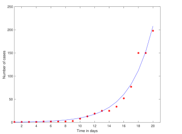
Figure 1. The number of infected for the SEIR non-structured model. The used parameters values are as in 3.2 .

Remark 3.1.

The model must be considered with care. The curve $I(t)$, as given by the SEIR model, predicts the total number of infected individuals (symptomatic and asymptomatic) at time $t$. However, to estimate the number of individuals that will need medical care, one needs to know the proportion between the reported and unreported cases. Estimates for the number of unreported cases can be found at [10] and the severity of the reported cases can be found at [4]. Asymptomatic cases can be as high as $75\%$ [3] of all cases; also, ratio estimates of reported to non reported cases goes from $1/1$ to $1/20$ [10]. These uncertainties must be taken into consideration when using the model to make numerical previsions. The emphasis of this paper is placed on understanding qualitatively efficient ways of controlling the epidemic.

Quarantines will be characterized by two values: the entrance rate $p$ and the exit rate $\lambda$. $p$ is composed of two terms, $\gamma_{q}$ and $\xi$. $\gamma_{q}$ is the average time it takes for a person to enter quarantine (see [8]) and $\xi$ is a dimensionless multiplicative factor representing the percentage of individuals that in fact voluntarily quarantine. With this notation

$$p=\frac{\xi}{\gamma_{q}}\,.$$

As an example, suppose that $70\%$ of the population quarantine in an interval of 2 days. Then $p=0.70/2=0.35$. It will be assumed that $p\in[0.0\,,\,0.40]\,.$ $p=0$ means that there is no quarantine. As in [8] it will be assumed that the time to leave quarantine will between 30 and 60 days; giving that $\lambda\in[1/60\,,\,1/30]$.

Remark 3.2.

For future reference we observe that, from definition, $p$ is smaller then the percentage of quarantined population.

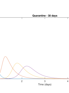
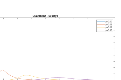
Figure 2. Prevalence curve for different quarantine efforts. The top figure assumes a 30 days quarantine and the bottom figure a 45 days quarantine.

The effect of the quarantine on the prevalence curve is twofold: it decreases the maximum $I(t)$ value and postpones the date of its occurrence. To assess the efficiency of the quarantine, the maximum of the prevalence curve and the time of its occurrence were calculated and are shown in Figure 3 .

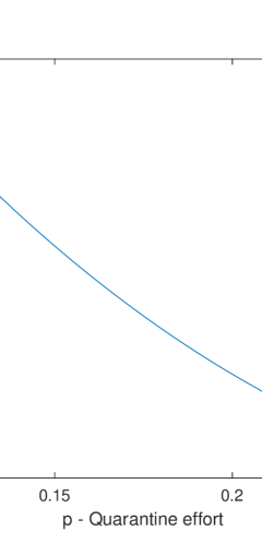
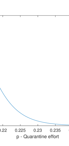
Figure 3. Maximum of infected as a function of the quarantine effort $p$. The figure on the right-hand side details the fast decrease after $p=0.21$ . Quarantine time is $30$ days.

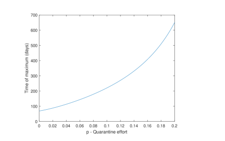
Figure 4. The time for the maximum of the epidemic curve as a function of the quarantine effort $p$. Quarantine time is 30 days.

The important feature on Figure 3 is the existence of a threshold value for the epidemic effort. For values greater than this critical value, the maximum number of infected decreases extremely fast and the maximum time essentially stabilizes. This is a common feature for all $p$ and $\lambda$ as shown in figure 5.

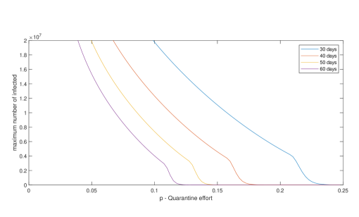
Figure 5. The maximum of the epidemic curve as a function of the quarantine effort $p$ for different quarantine values.

Critical values for quarantine efforts are clearly seen for the contour plots for the maximum number of infected. The white region on Figure 6 divides the parameter plane in two regions. The region above has a maximum number of infected smaller then $1\times 10^{6}$ infected (by the above rough estimates $\approx$ 5000 deaths ). The region below has larger numbers of infected (and of deaths). The level sets accumulate around a critical level set, showing again that, qualitatively, quarantines do work.

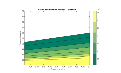
Figure 6. Level curves for the maximum number of infected as a function of quarantine effort and quarantine time.

4. Control strategies for the age-structured model

The control measures for the age structured model will be divided in two types. The first type controls the epidemic parameters ([2]). This will be made through an $R_{0}$ sensitivity analysis: the $R_{0}$ for the age structured model will be numerically determined and its parameter dependence will be investigated. The second type of control will be the age-oriented quarantines. The parameters $p_{i}$ determine the quarantine effort for each class. Due to the different classes weight on the population composition, and to the different epidemic parameters of each class, this study allows us to assess the impact of each class quarantine on the epidemic dynamics.

Before we proceed, we need to adjust the parameters for the structured model.

4.1. Data Fitting

There are 12 parameters to be determined for the structured model:

$$\sigma_{i}\,\,\,,\,\,\,\gamma_{i}\,\,\,\mbox{and}\,\,\,\beta_{ij}=\beta_{ji}\,\,\,\mbox{for}\,\,\,i,j=1,2,3\,.$$

The algorithm fits the parameters to the available data of Brazil’s total number of reported cases for the first 19 days of infection by a least squares method. The distance between the predicted curve

$$I(t)=I_{1}(t)+I_{2}(t)+I_{3}(t)$$

and the data curve is minimized. The initial parameters for the minimization search algorithm are based on the ones found for the unstructured SEIR model (3) taking into consideration the population percentage of each age class. Let $c_{i}$ be the population percentage of each class, that is (see Table 1), $c_{1}=0.402$, $c_{2}=0.505$ and $c_{3}=0.093$. The initial values for the interation are chosen as

$$\sigma_{i}=c_{i}\,\frac{\sigma^{*}_{i}}{3}\,\,\,\mbox{and}\,\,\,\gamma_{i}=c_{i}\,\frac{\gamma^{*}_{i}}{3}\,\,\,\mbox{for}\,\,\,i=1,2,3$$

and

$$\beta_{ij}=\beta^{*}\,\,\,\mbox{for}\,\,\,i\leq j=1,2,3\,,$$

The resulting values are listed in Table 3 and a plot of the daily number of infections and the number of reported cases is shown in Figure 7.

Table 3. Fitted parameters for the age-structured SEIR model without vital dynamics.

Parameter	Value	Parameter	Value
$\beta_{11}$	1.76168	$\sigma_{1}$	0.27300
$\beta_{12}$	0.36475	$\sigma_{2}$	0.58232
$\beta_{13}$	1.32468	$\sigma_{3}$	0.69339
$\beta_{22}$	0.63802	$\gamma_{1}$	0.06862
$\beta_{23}$	0.35958	$\gamma_{2}$	0.03317
$\beta_{33}$	0.57347	$\gamma_{3}$	0.35577

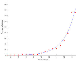
Figure 7. The number infected for the SEIR structured model. Parameter values as in Table 3

4.2. $R_{0}$ Analysis

$R_{0}$ is determined via the next generation approach [6]. It equals the spectral radius of $FV^{-1}$, where

$$F=\left(\begin{matrix}0&0&0&\beta_{11}\,S_{1}^{*}&\beta_{12}\,S_{1}^{*}&\beta_{31}\,S_{1}^{*}\\ \\ 0&0&0&\beta_{21}\,S_{2}^{*}&\beta_{22}\,S_{2}^{*}&\beta_{23}\,S_{2}^{*}\\ \\ 0&0&0&\beta_{31}\,S_{3}^{*}&\beta_{32}\,S_{3}^{*}&\beta_{33}\,S_{3}^{*}\\ \\ 0&0&0&0&0&0\\ \\ 0&0&0&0&0&0\\ \\ 0&0&0&0&0&0\\ \end{matrix}\right)$$

and

$$V=\left(\begin{matrix}D_{1}&0&0&0&0&0\\ \\ 0&D_{2}&0&0&0&0\\ \\ 0&0&D_{3}&0&0&0\\ \\ -\sigma_{1}&0&0&\tilde{D}_{1}&0&0\\ \\ 0&-\sigma_{2}&0&0&\tilde{D}_{2}&0\\ \\ 0&0&-\sigma_{3}&0&0&\tilde{D}_{3}\\ \end{matrix}\right),$$

where $D_{i}=\sigma_{i}+\mu_{i}$ and $\tilde{D}_{i}=\gamma_{i}+\mu_{i}+m_{i}$ for $i\in\{1,2,3\}$. Thus, $F\,V^{-1}$, is given by

$$FV^{-1}=\left(\begin{array}[]{cc}K_{11}&K_{12}\\ K_{21}&K_{31}\\ \end{array}\right),$$

where the block $K_{11}$ is

$$\left(\begin{matrix}\frac{\beta_{11}\,\sigma_{1}\,S_{1}^{*}}{\gamma_{1}\,(\sigma_{1}+\mu_{1})(\gamma_{1}+\mu_{1}+m_{1})}&\frac{\beta_{12}\,\sigma_{2}\,S_{1}^{*}}{\gamma_{2}\,(\sigma_{2}+\mu_{2})(\gamma_{2}+\mu_{2}+m_{2})}&\frac{\beta_{13}\,\sigma_{3}\,S_{1}^{*}}{\gamma_{3}\,(\sigma_{3}+\mu_{3})(\gamma_{3}+\mu_{3}+m_{3})}\\ \\ \frac{\beta_{21}\,\sigma_{1}\,S_{2}^{*}}{\gamma_{1}\,(\sigma_{1}+\mu_{1})(\gamma_{1}+\mu_{1}+m_{1})}&\frac{\beta_{22}\,\sigma_{2}\,S_{2}^{*}}{\gamma_{2}\,(\sigma_{2}+\mu_{2})(\gamma_{2}+\mu_{2}+m_{2})}&\frac{\beta_{23}\,\sigma_{3}\,S_{2}^{*}}{\gamma_{3}\,(\sigma_{3}+\mu_{3})(\gamma_{3}+\mu_{3}+m_{3})}\\ \\ \frac{\beta_{31}\,\sigma_{1}\,S_{3}^{*}}{\gamma_{1}\,(\sigma_{1}+\mu_{1})(\gamma_{1}+\mu_{1}+m_{1})}&\frac{\beta_{32}\,\sigma_{2}\,S_{3}^{*}}{\gamma_{2}\,(\sigma_{2}+\mu_{2})(\gamma_{2}+\mu_{2}+m_{2})}&\frac{\beta_{33}\,\sigma_{3}\,S_{3}^{*}}{\gamma_{3}\,(\sigma_{3}+\mu_{3})(\gamma_{3}+\mu_{3}+m_{3})}\\ \end{matrix}\right),\\$$

the block $K_{12}$ is

$$\left(\begin{array}[]{ccc}\frac{\beta_{11}\,S_{1}^{*}}{\gamma_{1}+\mu_{1}+m_{1}}&\frac{\beta_{12}\,S_{1}^{*}}{\gamma_{2}+\mu_{2}+m_{2}}&\frac{\beta_{13}\,S_{1}^{*}}{\gamma_{3}+\mu_{3}+m_{3}}\\ \\ \frac{\beta_{21}\,S_{2}^{*}}{\gamma_{1}+\mu_{1}+m_{1}}&\frac{\beta_{22}\,S_{2}^{*}}{\gamma_{2}+\mu_{2}+m_{2}}&\frac{\beta_{23}\,S_{2}^{*}}{\gamma_{3}+\mu_{3}+m_{3}}\\ \\ \frac{\beta_{31}\,S_{3}^{*}}{\gamma_{1}+\mu_{1}+m_{1}}&\frac{\beta_{32}\,S_{3}^{*}}{\gamma_{2}+\mu_{2}+m_{2}}&\frac{\beta_{33}\,S_{3}^{*}}{\gamma_{3}+\mu_{3}+m_{3}}\\ \end{array}\right)$$

and $K_{21}$ and $K_{22}$ are the $3\times 3$ zero matrix. Due to the block structure of $F\,V^{-1}$, its eigenvalues are easily calculated. However, due to the high number of parameters, their expression is too cumbersome to be of any analytical use. The sensitivity analysis is therefore computed numerically. Figures 8, 9, 10 and 11 show the $R_{0}$ parameter dependence.

Figure 8. $R_{0}$ as a $\gamma_{i}$ function. Different curves show which $\gamma_{i}$ is varying while the others are kept constant.

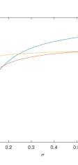
Figure 9. $R_{0}$ as a $\sigma_{i}$ function. Different curves show which $\sigma_{i}$ is varying while the others are kept constant.

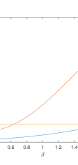
Figure 10. $R_{0}$ as a $\beta_{ii}$ function. Different curves show which $\beta_{ii}$ is varying while the others are kept constant.

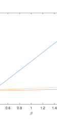
Figure 11. $R_{0}$ as a $\beta_{ij}\,\,i<j\,$ function. Different curves shows which $\beta_{ij}$ is varying while the others are kept constant.

The use of the parameters of the classical SIR model as control variables was studied at [1]. We will follow its interpretation. Measures as keeping social distance, wearing protective masks, washing hands, etc have the effect of reducing the contact rates $\beta_{ij}$. Identifying infected through tests, body temperature checks, etc and putting them into quarantine has the effect of increasing the removal rates $\gamma_{i}$. $\sigma_{i}$ is a parameter that can not be controlled.

The results can be summarized as follows:

i) Class 1 is the most sensitive to screening measures (see figure 8 ). Youngsters should be preferentially screened.

ii) Considering the direct contacts within the same class, class 2 is the more sensitive (see Figure 10 ). Social distance between adults has the biggest impact on $R_{0}$.

iii) For the direct contact between different class, $\beta_{12}$ has the greatest impact on $R_{0}$.

5. The effects of different quarantine policies

In this section we study the impacts of different quarantine strategies. The disease induced mortality rate was taken into account by considering the number of deaths as a fraction of the recovered class. Death rates for all age groups are estimated using the data from [4] (Table 4). As mentioned in Section 3, $I_{1}$, $I_{2}$ and $I_{3}$ include symptomatic and asymptomatic infected individuals as well as unreported cases, so death rates will be multiplied by a factor of $0.25$ (since only 25$\%$ of the infected are symptomatic [3]) and by $1/20$ (due to unreported cases [10]). This leaves us with a multiplicative factor of $\phi=0.25*(1/20)=0.0125$ to estimate the number of deaths. Since we will be working with relative proportions, the actual value of $\phi$ will be of no importance.

Table 4. Death rates for the age-structured model (data taken from [4]).

Age group	Number of cases	Deaths	$\%$ Death
1	350	1	$0.29\%$
2	9541	36	$0.38\%$
3	9068	768	$8.47\%$

With these values at hand, we can study the impact of a quarantine with parameters $\lambda$ and $p_{i}$, for $i\in\{1,2,3\}$. Calling $p$ the quarantine effort for the unstructured model, it is assumed that the total quarantine effort equals the effort for the non-structured model that is

$$p_{1}+p_{2}+p_{3}=p\,.$$

Remark 5.1.

As mentioned in 3.2, calling $q_{i}\,\,\,i=1,2,3$ the percentage of quarantined on each age class, it follows that

$$p<q_{1}+q_{2}+q_{3}\leq 1\,.$$

Four different choices for the $p_{i}$’s will be used, as detailed in Table 5. These are choices for the quarantine effort of each age group. Strategy S1 splits the effort equally among the three groups. Strategy S2 emphasizes a stronger isolation of the elderly (twice as much as the other groups). Strategy S3 enforces isolation of the youngsters and adults twice as much as it does for the elderly. Finally, strategy S4 doubles the quarantine effort on the adults in comparison to the others. To assess the efficiency of these different control strategies, for a fixed control effort $p$, each control strategy will be calculated for different quarantine times $\lambda\in\{1/30,1/45,1/60\}$.

Table 5. Quarantine strategies.

Strategy	Choices for the $p_{i}$
S1	$p_{1}=p/3$, $p_{2}=p/3$, $p_{3}=p/3$
S2	$p_{1}=p/6$, $p_{2}=p/6$, $p_{3}=2p/3$
S3	$p_{1}=2p/5$, $p_{2}=2p/5$, $p_{3}=p/5$
S4	$p_{1}=p/6$, $p_{2}=2p/3$, $p_{3}=p/6$

The estimation of the number of deaths can be made by multiplying the number of recovered at the end of the epidemic in each of the three age groups by the death rates from Table 4 and by the multiplicative factor $\phi$. However, due to parameters uncertainties and lack of estimations for the parameter $p$, a different approach is taken. We arbitrarily chose one of the values as unit and calculated all the other results proportionally. The results for $p=0.2$ are available in Table 6. (For reference only, the number of deaths chosen as unit was 2869).

Table 6. Proportion of deaths for each age group for different quarantine strategies and durations.

$\lambda$	Age group	S1	S2	S3	S4
	1	1	1.02	0.99	1.03
1/30	2	1.61	1.67	1.59	1.47
	3	7.20	6.43	7.46	7.51
	Total	9.81	9.12	10.04	10.01
	1	0.95	0.99	0.93	1.01
1/45	2	1.51	1.60	1.47	1.29
	3	6.77	5.75	7.18	7.26
	Total	9.23	8.34	9.58	9.56
	1	0.90	0.96	0.88	0.98
1/60	2	1.41	1.54	1.36	1.14
	3	6.38	5.21	6.90	7.01
	Total	8.69	7.71	9.14	9.13

One could argue that the optimal control would occur if we put all the quarantine effort in the isolation of the elderly and no isolation at all for youngsters and adults. With our terminology, this means considering a strategy S5 defined by $p_{1}=p_{2}=0$ and $p_{3}=p$. However, this leads to two main problems: first, due to the small percentage of the elder class the quarantine effort would be to small (in fact smaller then 0.1) to be of any significance. Second, it would allow for a much higher number of infected individuals (see Figure 12), hence a great increase in the total of hospitalizations, which would collapse the Health System. Therefore, to achieve better quarantine results, the total effort needs to include all age-groups, with more emphasis on the elderly since they have a higher fatality rate due to the disease.

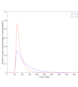
Figure 12. Plots of the total number of infected, as percentages of the total population, for strategies S2 and S5. The quarantine parameters were $p=0.2$ and $\lambda=1/60$.

Notice that strategy S2 is, by far, the best among these. All other strategies end up with, at least, 7.5$\%$ more deaths. We can also analyse the strategies by plotting them. Let $\mu_{i}$, $i\in\{1,2,3\}$, be the death rates from Table 4, so

$$\mathcal{D}_{j}(t)=\phi\sum_{i=1}^{3}\mu_{i}R_{i}(t)$$

converges to the total amount of deaths that result from strategy S_j, $j\in\{1,2,3,4\}$. Figure 13 plots the graphs of $\mathcal{D}_{j}(t)$, normalized by

$$\lim_{t\rightarrow\infty}\mathcal{D}_{2}(t),$$

produced by the four strategies for different values of $p$. Notice yet that, in all four cases, the strategy that produces the smallest limit value (hence the smallest death toll) is S2.

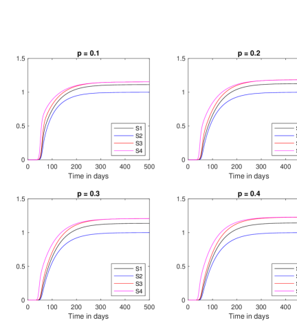
Figure 13. Plots of $\mathcal{D}_{j}(t)$ for $\lambda=\frac{1}{30}$, $j\in\{1,2,3,4\}$.

6. Conclusions

In this paper we introduced an age-structured SEIR model with a quarantine compartment. Three age classes were used: infants (0 to 19 years), adults (20 to 59 years) and elderly (60 to 100 years). First we studied the associated classical unstructured SEIR model without vital dynamics. The parameters were fitted by a least-square algorithm and the impact of the quarantine parameters $p$ and $\lambda$ were studied. Our main findings concern the existence of a numerical threshold value for the quarantine parameters: above a certain curve on the $(p,\lambda)$-plane, the maximum number of infected decreases in an accentuated way. This shows that an abrupt decline on the number of cases should be observed if the quarantine is being efficient. If this decline is not being observed, quarantine effort and time should be increased.

The parameters obtained for the unstructured SEIR model were used to adjust the parameters for the age-structured SEIR model. Using this data, the basic reproduction number $R_{0}$ was calculated and its dependence on the epidemic values was studied. Our findings for the $R_{0}$ analysis are as follows:

i) Class 1 is the most sensitive to screening measures (see Figure 8). Youngsters should be preferentially screened.

ii) Considering the direct contacts within the same class, class 2 is the more sensitive (see Figure 10 ). Social distance between adults has the biggest impact on $R_{0}$.

iii) For the direct contact between different class, $\beta_{12}$ has the greatest impact on $R_{0}$.

Finally we studied the impact of age-oriented campaigns considering different strategies and different values of $p$ for the total campaign effort. Recalling that $p$ is bounded by the percentage of quarantined population (see remarks 3.2 and 5.1), our findings show that the highest possible quarantine must be made, and then, this effort must concentrate on putting into quarantine the total of elders and assuring equal proportions of adults and youngsters.

References

- [1] Cesar Castilho, Optimal control of an epidemic through educational campaigns., Electronic Journal of Differential Equations 2006 (2006).
- [2] Carlos Castillo-Chavez, Herbert W Hethcote, Viggo Andreasen, Simon A Levin, and Wei M Liu, Epidemiological models with age structure, proportionate mixing, and cross-immunity, Journal of mathematical biology 27 (1989), no. 3, 233–258.
- [3] Michael Day, Covid-19: four fifths of cases are asymptomatic, china figures indicate., The BMJ (2020), https://www.bmj.com/content/369/bmj.m1375.
- [4] Centro de Coordinación de Alertas y Emergencias Sanitarias Gobierno España, Enfermedad por el coronavirus (covid-19)., 2020 (accessed April 4, 2020), https://www.mscbs.gob.es/profesionales/saludPublica/ccayes/alertasActual/nCov-China/documentos/Actualizacion_52_COVID-19.pdf.
- [5] Instituto Brasileiro de Geografia e Estatística, Sinopse do censo demográfico 2010, 2011, https://biblioteca.ibge.gov.br/visualizacao/livros/liv49230.pdf.
- [6] Odo Diekmann, Johan Andre Peter Heesterbeek, and Johan AJ Metz, On the definition and the computation of the basic reproduction ratio in models for infectious diseases in heterogeneous populations, Journal of mathematical biology 28 (1990), no. 4, 365–382.
- [7] Hisashi Inaba, Mathematical analysis of an age-structured sir epidemic model with vertical transmission, Discrete & Continuous Dynamical Systems-B 6 (2006), no. 1, 69.
- [8] Jiwei Jia, Jian Ding, Siyu Liu, Guidong Liao, Jingzhi Li, Ben Duan, Guoqing Wang, and Ran Zhang, Modeling the control of covid-19: Impact of policy interventions and meteorological factors, arXiv preprint arXiv:2003.02985 (2020).
- [9] Maia Martcheva, Introduction to epidemic modeling, An Introduction to Mathematical Epidemiology, Springer, 2015, pp. 9–31.
- [10] Timothy Russel, Using a delay adjusted case fatality ratio to estimate under reporting, 2020, https://cmmid.github.io/topics/covid19/severity/global_cfr_estimates.html.
- [11] Horst Thieme, Disease extinction and disease persistence in age structured epidemic models, Nonlinear Analysis, Theory, Methods and Applications 47 (2001), no. 9, 6181–6194.
- [12] Joseph T Wu, Kathy Leung, and Gabriel M Leung, Nowcasting and forecasting the potential domestic and international spread of the 2019-ncov outbreak originating in wuhan, china: a modelling study, The Lancet 395 (2020), no. 10225, 689–697.
- [13] Linhua Zhou, Yan Wang, Yanyu Xiao, and Michael Y Li, Global dynamics of a discrete age-structured sir epidemic model with applications to measles vaccination strategies, Mathematical biosciences 308 (2019), 27–37.
- [14] Yicang Zhou and Paolo Fergola, Dynamics of a discrete age-structured sis models, Discrete & Continuous Dynamical Systems-B 4 (2004), no. 3, 841.