Correlation lengths in the language of computable information

Abstract

Computable Information Density (CID), the ratio of the length of a losslessly compressed data file to that of the uncompressed file, is a measure of order and correlation in both equilibrium and nonequilibrium systems. Here we show that correlation lengths can be obtained by decimation, thinning a configuration by sampling data at increasing intervals and recalculating the CID. When the sampling interval is larger than the system’s correlation length, the data becomes incompressible. The correlation length and its critical exponents are thus accessible with no a-priori knowledge of an order parameter or even the nature of the ordering. The correlation length measured in this way agrees well with that computed from the decay of two-point correlation functions $g_{2}(r)$ when they exist. But the CID reveals the correlation length and its scaling even when $g_{2}(r)$ has no structure, as we demonstrate by “cloaking” the data with a Rudin-Shapiro sequence.

Physics, and indeed science in general, is a search to find and quantify correlations and order in nature. In many cases this organization is evident and quantifiable in terms of an order parameter which is identified with a broken symmetry. Such symmetry breaking is often associated with a phase transition at which the order parameter becomes finite, and a length scale for the persistence of the order which diverges as one approaches the transition. There are, however, systems in nature whose order we do not yet understand or for which we cannot define an order parameter in the conventional sense. Even in such cases, we may reasonably expect that there exist some as yet unidentified correlations, with associated length scales which may or may not diverge.

The basic idea we wish to exploit is the intimate connection between order and information: it takes less information to completely describe a system with correlations than an uncorrelated one. The basis for the quantification of these ideas can be found in information theory Cover and Thomas (2012), in particular the Shannon entropy Shannon (1948) and the Kolmogorov complexity Kolmogorov (1968); Chaitin (1966). In recent work Martiniani et al. (2019) we have introduced a quantitative measure, the Computable Information Density (CID), $\mathcal{K}\equiv\mathcal{L}(\mathbf{x})/L$, that is the binary code length, $\mathcal{L}(\mathbf{x})$, of a losslessly compressed file $\mathbf{x}$ (such as the microstate of a many-body system) divided by the uncompressed length $L$ (the number of degrees of freedom) of $\mathbf{x}$ , which is closely related to the Shannon and Kolmogorov measures, and which is an excellent approximant of the thermodynamic entropy, $S$, for equilibrium systems. In what follows we estimate the CID using the unrestricted Lempel-Ziv string matching algorithm (LZ77) Ziv and Lempel (1977); Shields (1999), a universal (i.e., requires no a-priori knowledge of the nature of the ensemble) and asymptotically optimal code (i.e., $\lim_{L\to\infty}\mathcal{K}=S$) Cover and Thomas (2012); Martiniani et al. (2019). CID reveals the nature of phase transitions (first or second order), the position of critical points, and the exponent of critical slowing down, for both equilibrium and nonequilibrium phase transitions. Here we wish to explore whether CID can be used to determine correlation lengths for such systems .

The standard method for computing the correlation length $\xi$ of a system is to calculate some correlation function, typically two-point, and see how it decays with distance. This presupposes that the order and proper correlation function is known. In this paper, we propose a method that does not require this knowledge, which is based on the fundamental idea that correlations reduce the CID of a system.

If a system consists of uncorrelated elements, the CID takes its maximum value. To exploit this, we sample a system on various length scales $\Delta$ by culling out degrees of freedom on smaller scales. In Fig. 1a-b we consider a 1D model of randomly placed hard rods of length $\ell=4$, while in Fig. 1c-d we have a 1D Ising model Ising (1925) at finite temperature and zero applied magnetic field. The diagrams in Fig. 1a and 1c show a respective configuration from each of the models, which we sample on every fourth site ($\Delta=4$). If $\Delta<\xi$, the remaining degrees of freedom still show correlations, albeit weakened, but if $\Delta>\xi$, all correlations are lost and the CID attains its maximal value. In the simplest cases e.g. for the 1D hard-rod model, to estimate $\xi$ we can simply look for the smallest value of $\Delta$ where the CID reaches its maximum. However, this is not always adequate e.g. in the 1D Ising model the CID approaches its maximum exponentially, so we find that in general it is better to study the way that the CID scales with $\Delta$ by collapsing the data. This procedure has the advantage of being independent of the system being analyzed.

(b)(a)0in-1.6in0.8in-1.6in

(d)(c)0in-1.6in0.8in-1.6in

Figure 1: Diagrams depict (a) 1D hard-rods of length $\ell=4$ and (c) 1D Ising configurations, their shuffled counterparts, and the result of decimation when the sampling interval is $\Delta=4$. (b) 1D hard rods, with lengths $\ell=2^{i}$ ($1\leq i\leq 6$), randomly distributed on a grid of length $L=2^{16+i}$, at fixed density $\rho\equiv N_{r}\ell/L=1/4$. Upon decimation at intervals $\Delta>\ell$, the configurations reduce to a random sequence. The main panel shows $Q(\Delta,\ell)$, dashed lines are exact solution to leading order (see Eq. S5 in SM Note (4)). Inset shows $\xi$ as computed from $Q(\Delta)$ and $g_{2}(r)$ taking $\xi$ to be the value where $Q(\xi)=0.025$ and where $g_{2}(\xi)$ is a its minimum (see SM Note (4)). (d) 1D Ising model of size $L=2^{20}$ simulated by Wolff algorithm Wolff (1989). We performed the same analysis as for panel $a$ but extracted $\xi$ by fitting the curves to exponential functions of the form $g_{2}(r)=g_{2}(0)\exp(-r/\xi)$ and ${Q}(\Delta)={Q}(1)\exp(-(\Delta-1)/\xi)$. Data were averaged over 200 equilibrium configurations. The black dashed lines show the theoretical scaling for $\xi$ with T. Inset shows the collapsed $Q(\Delta,T)$, along with the analytical solution Eq. 1 (red line).

In particular, we wish to study the quantity

$${Q}(\Delta)\equiv 1-\frac{\mathcal{K}(\Delta)}{\mathcal{K}_{\mathrm{shuf}}(\Delta)}$$ (1)

where we denoted the CID as $\mathcal{K}$, and the subscript ‘shuf’ refers to a configuration obtained by randomly shuffling all its degrees of freedom. Because a randomly shuffled configuration has no correlations, $\mathcal{K}_{\mathrm{shuf}}(\Delta)\geq\mathcal{K}(\Delta)$, and $0\leq{Q}\leq 1$.

The 1D hard-rod system consists of $N_{r}$ rods, each occupying $\ell$ contiguous sites, randomly distributed on a lattice of length $L$ sites. The fraction of occupied sites is $\rho=N_{r}\ell/L$. Configurations of the system are represented by strings $\{n_{j}\}$, where $j=1,2,\ldots,L$ and $n_{j}=1$ if site $j$ is occupied by a rod element, and $n_{j}=0$ if it is not. The trivial correlation length is $\ell$. Can we discover this by decimating configurations, computing their CID, and estimating $\xi_{\mathrm{CID}}$ from the value of $\Delta$ at which ${Q}(\Delta,\ell)\rightarrow 0$ for different values of $\ell$?

The decimated configurations are obtained by retaining the occupancies $n_{j\cdot\Delta}$ (with $j=1,2,\ldots,L/\Delta$) of a configuration, deleting all the others, and then rescaling the system by a factor $\Delta$. In Fig. 1b we plot $Q(\Delta)$ for several values of $\ell$, with $\xi_{\mathrm{CID}}$ vs. $\ell$ shown in the inset, along with the values of $\xi_{g_{2}}$ obtained by finding the minimum of the two-point correlation function $g_{2}(r)$ of the undecimated configurations (see SM ). Both correlation lengths are close in value to $\ell$ but differ numerically by a small factor. The data collapse, along with the exact result, showing that ${Q}(\rho,\Delta,\ell)\rightarrow 0$ linearly with $\Delta-\ell$ as $\Delta\rightarrow\ell$, are given in SM Note (4).

We next consider the equilibrium 1D Ising model, which has a transition at $T=0$. Both the entropy $S$ and $\xi$ may be solved for exactly Salinas (2001), and give

$${Q}(\Delta,\xi)=\frac{e^{-\Delta/\xi}\coth^{-1}\left(e^{\Delta/\xi}\right)+\frac{1}{2}\log\left(1-e^{-2\Delta/\xi}\right)}{\log(2)}$$ (2)

Here, ${Q}\rightarrow 0$ exponentially as ${Q}\sim e^{-2\Delta/\xi}$, making an extrapolation inadequate to determine $\xi_{\mathrm{CID}}$. Rather, we generate equilibrium spin configurations for different temperatures, decimate these configurations, calculate the CID to find ${Q}(\Delta)$, and then collapse them to a universal curve (inset of Fig. 1d). The collapse indicates that there is a single length scale $\xi$ in the problem and yields its temperature dependence. An exponential fit to a single curve ${Q}$ vs. $\Delta/\xi$ then gives the value of $\xi_{\text{CID}}$. $\xi_{\text{CID}}(T)$ and $\xi_{g_{2}}(T)$ are shown in Fig. 1d; both show the same $T$ dependence as the analytic $\xi(T)$.

Figure 2: 2D Ising model of size $L=2^{10}\times 2^{10}$ simulated by Wolff algorithm Wolff (1989). Correlation lengths $\xi$ extracted by fitting the pair-correlation function to $g_{2}(r)=g_{2}(0)\exp(-r/\xi)/r^{\eta}$ and ${Q}(\Delta)={Q}(1)\exp(-(\Delta-1)/\xi)/\Delta^{\theta}$. We find $\eta\approx 1/4$ and $\theta\approx 1/2$. The black dashed lines show the theoretical scaling $\xi\sim|T-T_{c}|/T_{c}$ with $T_{c}\approx 1.1345$. Data were averaged over 200 equilibrium configurations. Inset shows the collapse of the scaled $Q(\Delta,T)$.

Results in 2D for the $q$-state Potts models ($2\leq q\leq 8$) Potts (1952); Wu (1982) are shown in the SM Note (4). For $q=2$, this is the Ising model. Fig. 2 (inset) shows the collapse of ${Q}$ obtained by scaling the axes; this allows us to determine the critical exponent to be $\nu=1$, where $\xi(T)\propto(T-T_{c})^{-\nu}$. Fitting $Q(\Delta,T)$ at a single temperature gives us the numerical value of $\xi_{\mathrm{CID}}$, which is plotted alongside the value obtained from $g_{2}(r)$ in the main panel of Fig. 2. Notice that while decimating by $\Delta$ correctly yields configurations with correlation length $\xi/\Delta$, these are not equilibrium configurations with the same correlation length. This can be seen for instance from the fact that magnetization is invariant under decimation. In SM Note (4) we consider an alternative blocking transformation known as majority rule Kadanoff (1966), that yields valid equilibrium configurations and for which we can derive an exact expression for 2D Ising analogous to Eq. 2, and verify that there is good agreement between theory and numerical results in 2D.

We now consider the Conserved Lattice Gas (CLG), a dynamical nonequilibrium lattice model of the conserved directed percolation class Hinrichsen (2000). In the CLG (as illustrated in Fig. 3a) an occupied site is considered “active” if one of the nearest neighbors is also occupied (orange circles). Sites have a maximum occupancy of $1$ particle. At each time step, active sites are emptied stochastically by moving the particle to one of the empty neighboring sites (black arrows). The model has a continuous phase transition from a low density absorbing phase (where all sites are inactive) to a high density active phase where the dynamics persist forever. Configurations at the critical point are hyperuniform Hexner and Levine (2015); Torquato and Stillinger (2003). In 1D the critical density $\rho_{c}=1/2$ corresponds to a periodic arrangement where every other site is occupied (i.e., $101010\dots$). In Fig. 3b we show $\xi(\rho)$ as obtained both from CID and $g_{2}(r)$, as well as the scaling collapse of $Q(\Delta,\rho)$ for different densities (inset). We find that $\xi(\rho)$ diverges with the exponent $\nu=2$ for both measures as $\rho\to\rho_{c}$.

(b)(a)-0.1in-1.6in0.57in-1.6in

Figure 3: 1D Conserved Lattice Gas. (a) At time $t=0$ the system is in an active randomly sampled state (active sites in orange) and the possible moves prescribed by the dynamics are indicated by the arrows. When the density $\rho\leq\rho_{c}$ the system relaxes to an absorbing state with no active sites. (b) Correlation lengths $\xi$ for a system of size $L=2^{17}$ starting from randomly sampled states, extracted from $Q(\Delta)$ and $|g_{2}(r)|$ by taking $\xi$ to be the value where $Q(\xi)=0.05$ and $|g_{2}(\xi)|=0.05$. The black dashed lines show the fitted scaling $\xi\sim|(\rho-\rho_{c})/\rho_{c}|^{-2}$, where $\rho_{c}=0.5$. Inset shows the collapse of the scaled $Q(\Delta,\rho)$. Data were averaged over 15 independently generated configurations.

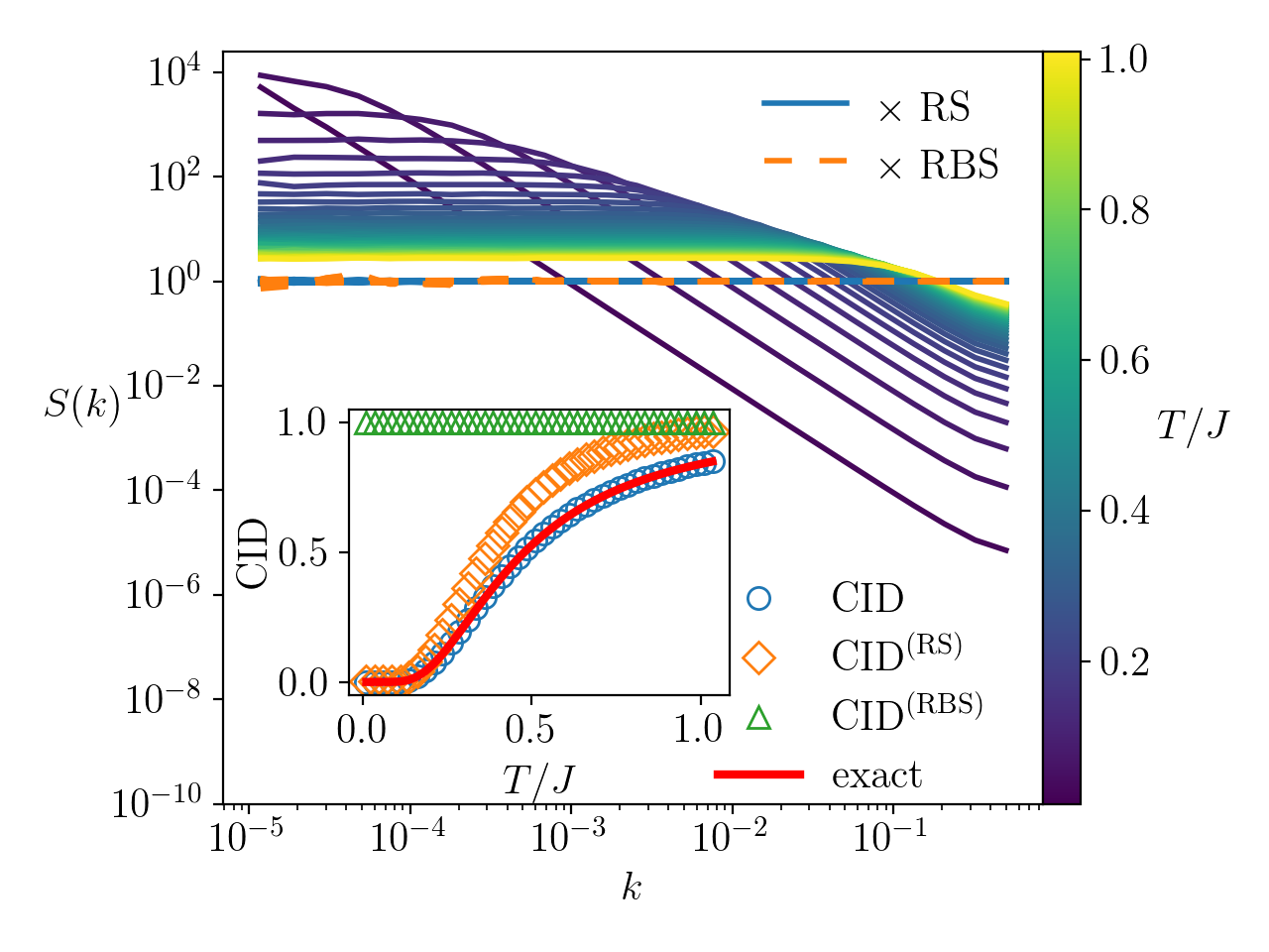
(a)-0.05in-1.5in

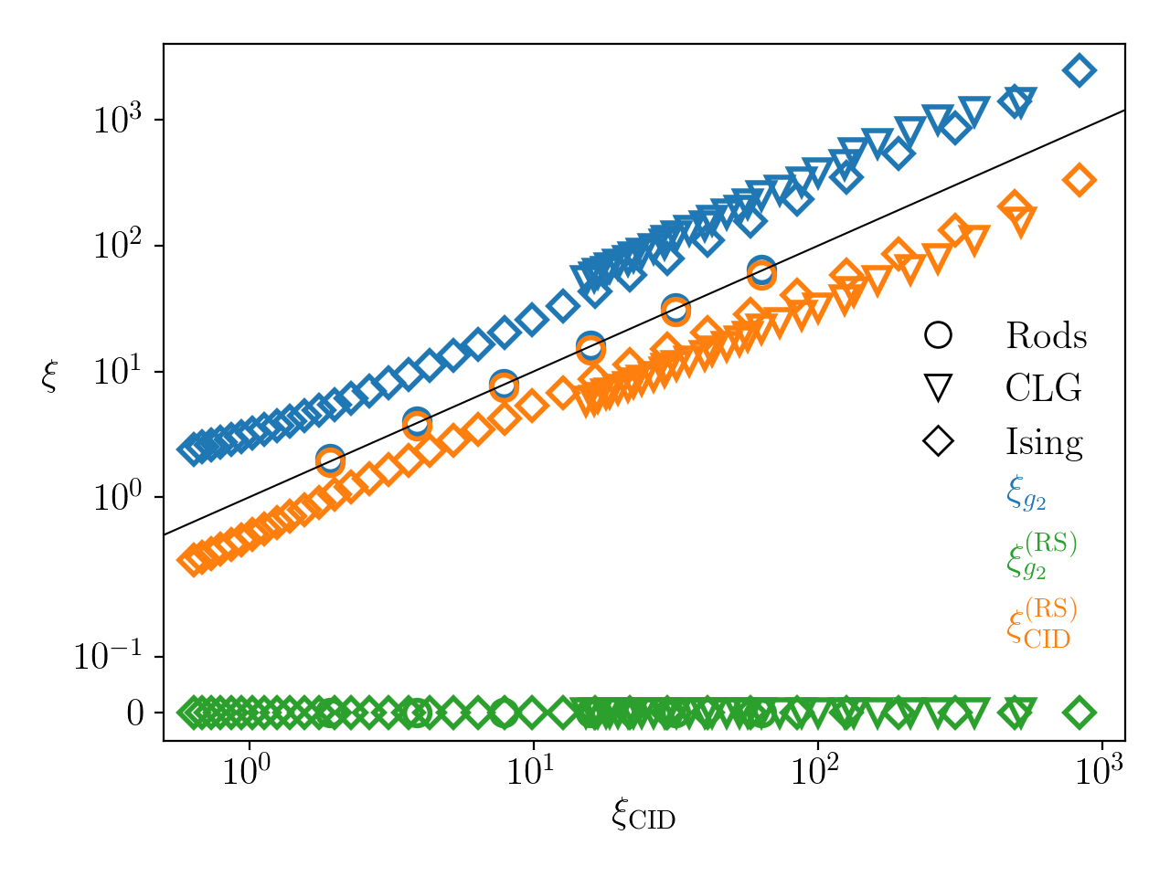
(b)-0.05in-1.5in

Figure 4: (a) Structure factor $S(k)$ for the 1D Ising model of size $L=2^{20}$. $S(k)$ is shown for the unaltered system, as well as for the Rudin-Shapiro, RS-cloaked, and Random Bernoulli Sequence (RBS) randomly-cloaked sequences, neither of which show any structure, indicating that all pair correlations have been destroyed. Inset: The CID as a function of T for the uncloaked and cloaked systems: The RS-cloaked system has nontrivial CID, but the randomly-cloaked system has maximum CID and is incompressible. Data were averaged over 200 equilibrium configurations. (b) Correlation lengths for the hard-rod, CLG, and 1D Ising systems, uncloaked (extracted from $g_{2}(r)$, in blue) and cloaked by RS (extracted from $g_{2}(r)$ and $Q(\Delta)$, in green and orange, respectively). The data is plotted against $\xi_{\mathrm{CID}}$, as measured by CID decimation of the uncloaked systems, so that a slope of 1 (solid line) means identical scaling for the RS-cloaked and uncloaked systems.

We now want to see whether CID decimation can measure correlation lengths in systems with no two-point correlations. To this end, we will “cloak” strings in two ways that destroy their two-point correlations. To do this, we multiply 1D Ising configurations by (i) a random Bernoulli sequence (RBS) of equal numbers of $\pm 1$, and (ii) the deterministic Rudin-Shapiro sequence Shapiro (1952); Allouche and Shallit (2003) (RS). Notice that this cloaking is exactly equivalent to studying two variants of the “Mattis glass”, with RS and RBS ground states Mattis (1976). Both of these sequences have $g_{2}(j,k)=\delta_{jk}$, but while for RS the Kolmogorov complexity and CID tend to zero as the sequence length increases, they are maximal for RBS Martiniani et al. (2019).

Multiplying a sequence with structure in its $g_{2}(r)$ (or, equivalently, its structure factor $S(k)$) by RBS will produce a maximally random sequence with $g_{2}(r)=0$ for $r\neq 0$ (and $S(k)=1$ ). Moreover, this will increase its CID , and cause all information about the original configuration to be lost (unless decoded by the identical random sequence). A similar multiplication by RS will remove all two-point correlations, also giving $g_{2}(r)=0$ (for $r\neq 0$) and $S(k)=1$, but will not appreciably change the Kolmogorov complexity of the original, since the RS itself has negligible Kolmogorov complexity. In this sense, “cloaking” by RS makes the sequence look random as far as $g_{2}(r)$ and $S(k)$ are concerned, while still retaining all the original information and order, although in a different form. We therefore expect that we should be able to recover the correlation length of the original, uncloaked system.

In Fig. 4a (inset) we show the CID for 1D Ising configurations at different temperatures, and for the same configurations cloaked by RS and by RBS. RBS-cloaked 1D Ising has a flat $\text{CID}=1$ indicating a correlation-less, maximally disordered system, but RS-cloaked 1D Ising retains much of its correlations. In the main panel of Fig. 4a we graph $S(k)$ for 1D Ising configurations, this shows increased correlations as T is lowered. Multiplying any configuration by RBS or RS gives $S(k)$=1. We now perform the decimation procedure to determine the correlation length of the cloaked configurations. In Fig. 4b we plot the correlation lengths for the RS-cloaked configurations as determined from CID decimation and from $g_{2}(r)$, vs. $\xi_{\mathrm{CID}}$ for the uncloaked 1D Ising configurations. For random cloaking, all information is lost, with no temperature dependence. However, for RS cloaking, although $\xi^{(RS)}_{g_{2}}(r)=0$, $\xi^{(RS)}_{\text{CID}}$ agrees well with the correlation length of the uncloaked 1D Ising system. Fig. 4b shows that similar conclusions hold also for the hard-rod and 1D CLG systems when cloaked by RS (see also SM Note (4)).

We note that RBS cloaking is analogous to the situation encountered in the analysis of static configurations of a square-lattice spin glass with random quenched disorder. In this case, without knowledge of the random couplings, the CID (or any other static estimator) would not be able to detect the order of an individual configuration because (like for RBS) individual configurations exhibit no correlations (and therefore are not compressible). It might, however, be possible to extract a correlation length by CID when considering the dynamics of the systems, viz. whole trajectories rather than individual configurations. We also argue that because structural glasses lack quenched disorder Karmakar and Parisi (2013), the CID may be an effective tool for the analysis of the glass transition, e.g. in soft sphere systems, given a sufficiently accurate CID estimator for continuum two and three dimensional systems.

CID decimation presents a simple and general method for finding the correlation length of equilibrium and nonequilibrium systems, or in fact of any temporal or spatial array (e.g. a sequence or an image), with no a-priori knowledge of a possible order parameter, as well as in systems where two-point correlations are uninformative. We expect that this technique may lead to the discovery of order and aid in the quantification of correlation lengths in a wealth of new systems.