Exact Single-Source SimRank Computation on Large Graphs

Abstract.

SimRank is a popular measurement for evaluating the node-to-node similarities based on the graph topology. In recent years, single-source and top-$k$ SimRank queries have received increasing attention due to their applications in web mining, social network analysis, and spam detection. However, a fundamental obstacle in studying SimRank has been the lack of ground truths. The only exact algorithm, Power Method, is computationally infeasible on graphs with more than $10^{6}$ nodes. Consequently, no existing work has evaluated the actual trade-offs between query time and accuracy on large real-world graphs.

In this paper, we present ExactSim, the first algorithm that computes the exact single-source and top-$k$ SimRank results on large graphs. With high probability, this algorithm produces ground truths with a rigorous theoretical guarantee. We conduct extensive experiments on real-world datasets to demonstrate the efficiency of ExactSim. The results show that ExactSim provides the ground truth for any single-source SimRank query with a precision up to 7 decimal places within a reasonable query time.

1. Introduction

Computing link-based similarity is an overarching problem in graph analysis and mining. Amid the existing similarity measures (page1999pagerank, ; xi2005simfusion, ; zhao2009p, ; zhang2015panther, ), SimRank has emerged as a popular metric for assessing structural similarities between nodes in a graph. SimRank was introduced by Jeh and Widom (JW02, ) to formalize the intuition that “two pages are similar if they are referenced by similar pages.” Given a directed graph $G=(V,E)$ with $n$ nodes $\{v_{1},\ldots,v_{n}\}$ and $m$ edges, the SimRank matrix $S$ defines the similarity between any two nodes $v_{i}$ and $v_{j}$ as follows:

(1) $$S(i,j)=\begin{cases}1,&\text{for $i=j$;}\\ {\displaystyle\sum_{v_{i^{\prime}}\in\mathcal{I}(v_{i})}{\sum_{v_{j^{\prime}}\in\mathcal{I}(v_{j})}{c\cdot S(i^{\prime},j^{\prime})\over d_{in}(v_{i})\cdot d_{in}(v_{j})}}},&\text{for $i\neq j$.}\end{cases}$$

Here, $c$ is a decay factor typically set to 0.6 or 0.8 (JW02, ; LVGT10, ). $\mathcal{I}(v_{i})$ denotes the set of in-neighbors of $v_{i}$, and $d_{in}(v_{i})$ denotes the in-degree of $v_{i}$. SimRank aggregates similarities of multi-hop neighbors of $v_{i}$ and $v_{j}$ to produce high-quality similarity measure, and has been adopted in various applications such as recommendation systems (li2013mapreduce, ), link prediction (lu2011link, ), and graph embeddings (tsitsulin2018verse, ).

A fundamental obstacle for studying SimRank is the lack of ground truths on large graphs. Currently, the only methods that compute the SimRank matrix is Power Method and its variations (JW02, ; lizorkin2010accuracy, ), which inherently takes $O(n^{2})$ space and at least $O(n^{2})$ time as there are $O(n^{2})$ node pairs in the graphs. This complexity is infeasible on large graphs ($n\geq 10^{6}$). Consequently, the majority of recent works (KMK14, ; MKK14, ; TX16, ; FRCS05, ; LeeLY12, ; LiFL15, ; SLX15, ; YuM15b, ; jiang2017reads, ; liu2017probesim, ; wei2019prsim, ) focus on single-source and top-$k$ queries. Given a source node $v_{i}$, a single-source query asks for the SimRank similarity between every node and $v_{i}$, and a top-$k$ query asks for the $k$ nodes with the highest SimRank similarities to $v_{i}$. Unfortunately, computing ground truths for the single-source and top-$k$ queries on large graphs still remains an open problem. To the best of our knowledge, Power Method is still the only way to obtain exact single-source and top-$k$ results, which is not feasible on large graphs. Due to the hardness of exact computation, existing works on single-source and top-$k$ queries focus on approximate computations with efficiency and accuracy guarantees.

The lack of ground truths has severely limited our understanding towards SimRank and SimRank algorithms. First of all, designing approximate algorithms without the ground truths is like shooting in the dark. Most existing works take the following approach: they evaluate the accuracy on small graphs where the ground truths can be obtained by the Power Method with $O(n^{2})$ cost. Then they report the efficiency/scalability results on large graphs with consistent parameters. This approach is flawed for the reason that consistent parameters may still lead to unfair comparisons. For example, some of the existing methods generate a fixed number of random walks from each node, while others fix the maximum error $\varepsilon$ and generate ${\log n\over\varepsilon^{2}}$ random walks from each node. If we increase the graph size $n$, the comparison becomes unfair as the latter methods require more random walks from each node. Secondly, it is known that the structure of large real-world graphs can be very different from that of small graphs. Consequently, the accuracy results on small graphs can only serve as a rough guideline for accessing the actual error of the algorithms in real-world applications. We believe that the only right way to evaluate the effectiveness of a SimRank algorithm is to evaluate its results against the ground truths on large real-world graphs.

Exact Single-Source SimRank Computation. In this paper, we study the problem of computing the exact single-source SimRank results on large graphs. A key insight is that exactness does not imply absolutely zero error. This is because SimRank values may be infinite decimals, and we can only store these values with finite precision. Moreover, we note that the ground truths computed by Power Method also incur an error of at most $c^{L}$, where $L$ is the number of iterations in Power Method. In most applications, $L$ is set to be large enough such that $c^{L}$ is smaller than the numerical error and thus can be ignored. In this paper, we aim to develop an algorithm that answers single-source SimRank queries with an additive error of at most $\varepsilon_{min}=10^{-7}$. Note that the float type in various programming languages usually support precision of up to 6 or 7 decimal places, so by setting $\varepsilon_{min}=10^{-7}$, we guarantee the algorithm returns the same answer as the ground truths in the float type. As we shall see, this precision is extremely challenging for existing methods. To make the exact computation possible, we are also going to allow a small probability to fail. We define the probabilistic exact single-source SimRank algorithm as follows.

Definition 0.

With probability at least $1-1/n$, for every source node $v_{i}\in V$, a probabilistic exact single-source SimRank algorithm answers the single-source SimRank query of $v_{i}$ with additive error of at most $\varepsilon_{min}=10^{-7}$.

Our Contributions. In this paper, we propose ExactSim, the first algorithm that enables probabilistic exact single-source SimRank queries on large graphs. We show that existing single-source methods share a common complexity term $O\left({n\log n\over\varepsilon_{min}^{2}}\right)$, and thus are unable to achieve exactness on large graphs. However, ExactSim runs in $O\left({\log n\over\varepsilon_{min}^{2}}+m\log{1\over\varepsilon_{min}}\right)$ time, which is feasible for both large graph size $m$ and small error guarantee $\varepsilon_{min}$. We also apply several non-trivial optimization techniques to reduce the query cost and space overhead of ExactSim. In our empirical study, we show that ExactSim is able to compute the ground truth with a precision of up to 7 decimal places within one hour on graphs with billions of edges. Hence, we believe ExactSim is an effective tool for producing the ground truths for single-source SimRank queries on large graphs.

2. Preliminaries and Related Work

In this section, we review the state-of-the-art single-source SimRank algorithms. Our ExactSim algorithm is largely inspired by three prior works: Linearization (MKK14, ), PRSim  (wei2019prsim, ) and pooling (liu2017probesim, ), and we will describe them in details. Table 1 summaries the notations used in this paper.

Table 1. Table of notations.

Notation	Description
$n,m$	the numbers of nodes and edges in $G$
$\mathcal{I}(v_{i}),\mathcal{O}(v_{i})$	the in/out-neighbor set of node $v_{i}$
$S,S(i,j)$	the SimRank matrix and the SimRank similarity of $v_{i}$ and $v_{j}$
$c$	the decay factor in the definition of SimRank
$\varepsilon,\varepsilon_{min}$	additive error parameter and error required for exactness ($\varepsilon_{min}=10^{-7}$)
$P$, $D$	the transition matrix and the diagonal correction matrix
$\vec{\pi}_{i},\vec{\pi}_{i}^{\ell},$	the Personalized PageRank and $\ell$-hop Personalized PageRank vectors of node $v_{i}$
$\vec{h}_{i}^{\ell}$	the $\ell$-hop Hitting Probability vector of $v_{i}$

MC (FR05, ) A popular interpretation of SimRank is the meeting probability of random walks. In particular, we consider a random walk from node $u$ that, at each step, moves to a random in-neighbor with probability $\sqrt{c}$, and stops at the current node with probability $1-\sqrt{c}$. Such a random walk is called a $\sqrt{c}$-walk. Suppose we start a $\sqrt{c}$-walk from node $v_{i}$ and a $\sqrt{c}$-walk from node $v_{j}$, we call the two $\sqrt{c}$-walks meet if they visit the same node at the same step. It is known (TX16, ) that

(2) $$S(i,j)=\Pr[\textrm{two }\sqrt{c}\textrm{-walks from }v_{i}\textrm{ and }v_{j}\textrm{ meet}].$$

MC makes use of this equation to derive a Monte-Carlo algorithm for computing single-source SimRank. In the preprocessing phase, we simulate $R$ $\sqrt{c}$-walks from each node in $V$. Given a source node $v_{i}$, we compare the $\sqrt{c}$-walks from $v_{i}$ and from each node $v_{j}\in V$, and use the fraction of $\sqrt{c}$-walks that meet as an estimator for $S(i,j)$. By standard concentration inequalities, the maximum error is bounded by $\varepsilon$ with high probability if we set $R=O\left({\log n\over\varepsilon^{2}}\right)$, leading to a preprocessing time of $O\left({n\log n\over\varepsilon^{2}}\right)$.

Linearization and ParSim. Given a graph $G=(V,E)$, let $P$ denote the (reverse) transition matrix, that is, $P(i,j)=1/d_{in}(v_{j})$ for $v_{i}\in\mathcal{I}(v_{j})$ and $P(i,j)=0$ otherwise. Let $S$ denote the SimRank matrix with $S(i,j)=s(v_{i},v_{j})$. It is shown in two independent works, Linearization (MKK14, ) and ParSim (yu2015efficient, ), that $S$ can be expressed as the following linear summation:

(3) $$S=\sum_{\ell=0}^{+\infty}c^{\ell}\left(P^{\ell}\right)^{\top}DP^{\ell},$$

where $D$ is the diagonal correction matrix with each diagonal element $D(k,k)$ taking value from $1-c$ to $1$. Consequently, a single-source query for node $v_{i}$ can be computed by

(4) $$S\cdot\vec{e_{i}}=\sum_{\ell=0}^{+\infty}c^{\ell}\left(P^{\ell}\right)^{\top}DP^{\ell}\cdot\vec{e_{i}},$$

where $\vec{e_{i}}$ denotes the one-hot vector with the $i$-th element being $1$ and all other elements being $0$. Assuming the diagonal matrix $D$ is correctly given, the single-source query for node $v_{i}$ can be computed by

(5) $$S_{L}\cdot\vec{e_{i}}=\sum_{\ell=0}^{L}c^{\ell}\left(P^{\ell}\right)^{\top}DP^{\ell}\cdot\vec{e_{i}},$$

where $L$ is the number of iterations. After $L$ iterations, the additive error reduces to $c^{L}$, so setting $L=O\left(\log{1\over\varepsilon}\right)$ is sufficient to guarantee a maximum error of $\varepsilon$. At the $\ell$-th iterations, the algorithms performs $2\ell+1$ matrix-vector multiplications to calculate $c^{\ell}\left(P^{\ell}\right)^{\top}DP^{\ell}\cdot\vec{e_{i}}$, and each matrix-vector multiplication takes $O(m)$ time. Consequently, the total query time is bounded by $O\left(\sum_{\ell=1}^{L}m\ell\right)=O(mL^{2})=O\left(m\log^{2}{1\over\varepsilon}\right)$. (MKK14, ) and (yu2015efficient, ) also show that if we first compute and store the transition probability vectors $\vec{u}_{i}=P^{\ell}\cdot\vec{e_{i}}$ for $\ell=0,\ldots,L$, then we can use the following equation to compute

(6) $$S_{L}\cdot\vec{e_{i}}=D\cdot\vec{u}_{0}+cP^{\top}(D\cdot\vec{u}_{1}+\cdots+cP^{\top}(D\cdot\vec{u}_{T-1}+cP^{\top}\cdot D\cdot\vec{u}_{T})\cdots),$$

However, this optimization requires a memory size of $O(nL)\\ =O\left(n\log{1\over\varepsilon}\right)$, which is usually several times larger than the graph size $m$. Therefore, (MKK14, ) only uses the $O\left(m\log^{2}{1\over\varepsilon}\right)$ algorithm in the experiments.

Besides the large space overhead, another problem with Linearization and ParSim is that the diagonal correction matrix $D$ is hard to compute. Linearization (MKK14, ) formulates $D$ as the solution to a linear system, and propose a Monte Carlo solution that takes $O\left({n\log n\over\varepsilon^{2}}\right)$ to derive an $\varepsilon$-approximation of $D$. On the other hand, ParSim directly sets $D=(1-c)I$, where $I$ is the identity matrix. This approximation basically ignores the first meeting constraint and has been adopted in many other SimRank works (FNSO13, ; He10, ; Yu13, ; Li10, ; Yu14, ; YuM15b, ; KMK14, ). It is shown that the similarities calculated by this approximation are different from the actual SimRank (KMK14, ). However, the quality of this approximation is still a myth due to the lack of ground truths on large graphs.

PRSim (wei2019prsim, ) introduces a partial indexing and a probe algorithm. Let $\vec{\pi}^{\ell}_{i}=(1-\sqrt{c})\vec{h}_{i}^{\ell}=(1-\sqrt{c})\left(\sqrt{c}P\right)^{\ell}\cdot\vec{e}_{i}$ denote the $\ell$-hop Personalize PageRank vector of $v_{i}$. In particular, $\vec{\pi}_{i}^{\ell}(k)$ is the probability that a $\sqrt{c}$-walk from node $v_{i}$ stops at node $v_{k}$ in exactly $\ell$ steps. PRSim suggests that equation (4) can be re-written as

(7) $$S(i,j)={1\over(1-\sqrt{c})^{2}}\sum_{\ell=0}^{\infty}\sum_{k=1}^{n}\vec{\pi}_{i}^{\ell}(k)\cdot\vec{\pi}_{j}^{\ell}(k)\cdot D(k,k).$$

PRSim precomputes $\vec{\pi}_{j}^{\ell}(k)$ with additive error $\varepsilon$ for each $\ell$ and $v_{j},v_{k}\in V$, using a local push algorithm (AndersenCL06, ). To avoid overwhelming space overhead, PRSim only precomputes $\vec{\pi}_{j}^{\ell}(k)$ for a small subset of $v_{k}$. Furthermore, PRSim computes $D$ by estimating the product $\vec{\pi}_{i}^{\ell}(k)\cdot D(k,k)$ together with an $O\left({\log n\over\varepsilon^{2}}\right)$ time Monte-Carlo algorithm. Finally, PRSim proposes a new Probe algorithm that samples each node $v_{j}$ according to $\vec{\pi}_{j}^{\ell}(k)$. The average query time of PRSim is bounded by $O\left({n\cdot\sum_{k=1}^{n}\vec{\pi}(k)^{2}\over\varepsilon^{2}}\log n\right)$, where $\vec{\pi}(k)$ denotes the PageRank of $v_{k}$. It is well-known that on scale-free networks, the PageRank vector $\vec{\pi}$ follows the power-law distribution, and thus $\|\vec{\pi}\|^{2}=\sum_{k=1}^{n}\vec{\pi}(k)^{2}$ is a value much smaller than $1$. However, for worst-case graphs or even some ”bad” source nodes on scale-free networks, the running time of PRSim remains $O\left({n\log n\over\varepsilon^{2}}\right)$.

2.1. Other Related Work

Besides the state-of-the-art methods that we discuss above, there are several other techniques for SimRank computation, which we review in the following. Power method (JW02, ) is the classic algorithm that computes all-pair SimRank similarities for a given graph. Let $S$ be the SimRank matrix such that $S_{ij}=s(i,j)$, and $P$ be the transition matrix of $G$. Power method recursively computes the SimRank Matrix $S$ using the formula (KMK14, ) $S=(cP^{\top}SP)\vee I,$ where $\vee$ is the element-wise maximum operator. Several follow-up works (LVGT10, ; YZL12, ; YuJulie15gauging, ) improve the efficiency or effectiveness of the power method in terms of either efficiency or accuracy. However, these methods still incur $O(n^{2})$ space overheads, as there are $O(n^{2})$ pairs of nodes in the graph. For single-source queries, READS (jiang2017reads, ) and TSF  (SLX15, ) are MC-based algorithms supporting dynamic graphs. Both of them incurs of $O\left({n\log n\over\varepsilon^{2}}\right)$ query time for $\varepsilon$ additive error. SLING (TX16, ) is an index-based SimRank algorithm that support fast single-source and top-$k$ queries on static graphs. Its preprocessing phase using $O\left({n\log n\over\varepsilon^{2}}\right)$ time which is infeasible for large graphs. ProbeSim (liu2017probesim, ) and TopSim (LeeLY12, ) are both index-free solutions based on local exploitation. Their query time is also bounded by $O\left({n\log n\over\varepsilon^{2}}\right)$. Besides, Li et al. (LiFL15, ) propose a distributed version of the Monte Carlo approach in (FRCS05, ), but it achieves scalability at the cost of significant computation resources. Finally, there is existing work on SimRank similarity join (TaoYL14, ; MKK15, ; ZhengZF0Z13, ), variants of SimRank (AMC08, ; FR05, ; Lin12, ; YuM15a, ; ZhaoHS09, ) and graph applications (bhuiyan2018representing, ; ye2018using, ), but the proposed solutions are inapplicable for top-$k$ and single-source SimRank queries.

Pooling. Finally, pooling (liu2017probesim, ) is an experimental method for evaluating the accuracy of top-$k$ SimRank algorithms without the ground truths. Suppose the goal is to compare the accuracy of top-$k$ queries for $\ell$ algorithms $A_{1},\ldots,A_{\ell}$. Given a query node $v_{i}$, we retrieve the top-$k$ nodes returned by each algorithm, remove the duplicates, and merge them into a pool. Note that there are at most $\ell k$ nodes in the pool. Then we estimate $S(i,j)$ for each node $v_{j}$ in the pool using the Monte Carlo algorithm. We set the number of random walks to be $O\left({\log n\over\varepsilon_{min}^{2}}\right)$ so that we can obtain the ground truth of $S(i,j)$ with high probability. After that, we take the $k$ nodes with the highest SimRank similarity to $v_{i}$ from the pool as the ground truth of the top-$k$ query, and use this “ground truth” to evaluate the precision of each of the $\ell$ algorithms. Note that the set of these $k$ nodes is not the actual ground truth. However, it represent the best possible $k$ nodes that can be found by the $\ell$ algorithms that participate in the pool and thus can be used to compare the quality of these algorithms.

Although pooling is proved to be effective in our scenario where ground truths are hard to obtain, it has some drawbacks. First of all, the precision results obtained by pooling are relative and thus cannot be used outside the pool. This is because the top-$k$ nodes from the pool are not the actual ground truths. Consequently, an algorithm that achieves $100\%$ precision in the pool may have a precision of $0\%$ when compared to the actual top-$k$ result. Secondly, the complexity of pooling $\ell$ algorithms is $O\left({\ell k\log n\over\varepsilon_{min}^{2}}\right)$, so pooling is only feasible for evaluating top-$k$ queries with small $k$. In particular, we cannot use pooling to evaluate the single-source queries on large graphs.

2.2. Limitations of Existing Methods

We now analyze the reasons why existing methods are unable to achieve exactness (a.k.a an error of at most $\varepsilon_{min}=10^{-7}$). First of all, ParSim ignores the first meeting constraint and thus incurs large errors. For other methods that enforce the first meeting constraint, they all incur a complexity term of $O\left({n\log n\over\varepsilon^{2}}\right)$, either in the preprocessing phase or in the query phase. In particular, SLING and Linearization simulate $O\left({n\log n\over\varepsilon^{2}}\right)$ random walks to estimate the diagonal correction matrix $D$. For ProbeSim, MC, READS and PRSim, this complexity is causing by simulating random walks in the query phase or the preprocessing phase. The $O\left({n\log n\over\varepsilon^{2}}\right)$ complexity is infeasible for exact SimRank computation on large graphs, since it combines two expensive terms $n$ and ${1\over\varepsilon_{min}^{2}}$. As an example, we consider the IT dataset used in our experiment, with $4*10^{7}$ nodes and over1 billion edges. In order to achieve a maximum error of $\varepsilon_{min}=10^{-7}$, we need to simulate ${n\log n\over\varepsilon^{2}}\approx 10^{23}$ random walks. This may take years, even with parallelization on a cluster of thousands of machines.

3. The ExactSim Algorithm

In this section, we present ExactSim, a probabilistic algorithm that computes the exact single-source SimRank results within reasonable running time. We first present a basic version of ExactSim, and then introduce some more advanced techniques to optimize the query and the space cost.

3.1. Basic ExactSim Algorithm

Our ExactSim algorithm is largely inspired by three prio works: pooling (liu2017probesim, ), Linearization (MKK14, ) and PRSim  (wei2019prsim, ). We now discuss how ExactSim extends from these existing methods in details. These discussions will also reveal the high level ideas of the ExactSim algorithm.

1. Despite its limitations, pooling (liu2017probesim, ) provides a key insight for achieving exactness: while an $O\left({n\log n\over\varepsilon^{2}}\right)$ algorithm is not feasible for exact SimRank computation on large graphs, we can actually afford an $O\left({\log n\over\varepsilon^{2}}\right)$ algorithm. The ${1\over\varepsilon^{2}}$ term is still expensive for $\varepsilon=\varepsilon_{min}=10^{-7}$, however, the new complexity reduces the dependence on the graph size $n$ to logarithmic, and thus achieves very high scalability.

2. Linearization (MKK14, ) and ParSim (yu2015efficient, ) show that if the diagonal correction matrix $D$ is correctly given, then we can compute the exact single-source SimRank results in $O\left(m\log_{1\over c}{1\over\varepsilon_{min}}\right)$ time and $O\left(n\log_{1\over c}{1\over\varepsilon_{min}}\right)$ extra space. For typical setting of $c$ ($0.6$ to $0.8$), the number of iterations $\log_{1\over c}{1\over\varepsilon_{min}}=\log{10^{7}}\leq 73$ is a constant, so this complexity is essentially the same as that of performing BFS multiple times on the graphs. The scalability of the algorithm is confirmed in the experiments of (yu2015efficient, ), where $D$ is set to be $(1-c)I$. Moreover, the exact algorithms (page1999pagerank, ) for Personalized PageRank and PageRank also incurs a running time of $O\left(m\log{1\over\varepsilon_{min}}\right)$, and has been widely used for computing ground truths on large graphs.

3. While the $O\left({n\log n\over\varepsilon^{2}}\right)$ complexity seems unavoidable as we need to estimate each entry in the diagonal correction matrix $D$ with additive error $\varepsilon$, PRSim (wei2019prsim, ) shows that it only takes $O\left({\log n\over\varepsilon^{2}}\right)$ time to estimate the product $\vec{\pi}_{i}^{\ell}(k)\cdot D(k,k)$ with additive error $\varepsilon$ for each $k=1,\ldots,n$ and $\ell=0,\ldots,\infty$, where $\vec{\pi}_{i}^{\ell}$ is the $\ell$-hop Personalized PageRank vector of $v_{i}$. This result provides two crucial observations: 1) It is possible to answer an single-source query without an $\varepsilon$-approximation of each $D(k,k)$; 2) The accuracy of each $D(k,k)$ should depend on $\vec{\pi}_{i}(k)$, the Personalized PageRank of $v_{k}$ with respect to the source node $v_{i}$.

We combine the ideas of PRSim and Linearization/ParSim to derive the basic ExactSim algorithm. Given an error parameter $\varepsilon$, ExactSim fixes the total number of $\sqrt{c}$-walk samples to be $R=O\left({\log n\over\varepsilon^{2}}\right)$, and distribute a fraction of $R\vec{\pi}_{i}(k)$ samples (note that $\sum_{k=1}^{n}\vec{\pi}_{i}(k)=1$) to estimate $D(k,k)$. It performs Linearization/ParSim with the estimated $D$ to obtain the single-source result. The algorithm runs in $O\left({\log n\over\varepsilon^{2}}+m\log{1\over\varepsilon}\right)$ time and uses $O\left(n\log{1\over\varepsilon}\right)$ extra space. Since both complexity terms $O\left(\log n\over\varepsilon^{2}\right)$ and $O\left(m\log{1\over\varepsilon}\right)$ are feasible for $\varepsilon_{min}=10^{-7}$ and large graph size $m$, we have a working algorithm for exact single-source SimRank queries on large graphs.

Input: Graph $G$ with transition matrix $P$, source node $v_{i}$, maximum error $\varepsilon$

Output: Estimated single-source SimRank vector $S\cdot\vec{e_{i}}$

1 $L=\left\lceil\log_{1\over c}{2\over\varepsilon}\right\rceil$;

2 $\vec{\pi}_{i}^{0},\vec{\pi}_{i}=(1-\sqrt{c})\vec{e}_{i}$;

3 for $\ell$ from $1$ to $L$ do

4       $\vec{\pi}_{i}^{\ell}=\sqrt{c}P\cdot\vec{\pi}_{i}^{\ell-1}$;

5       $\vec{\pi}_{i}=\vec{\pi}_{i}+\vec{\pi}^{\ell}$;

6      

7$R={6\log n\over(1-\sqrt{c})^{4}\varepsilon^{2}}$;

8 for $k$ from $1$ to $n$ do

9       Invoke Algorithm 2 with $R(k)=\lceil R\cdot\vec{\pi}_{i}(k)\rceil$ to obtain an estimator $\hat{D}(k,k)$ for $D(k,k)$;

10      

11$\vec{s}^{0}={1\over 1-\sqrt{c}}\hat{D}\cdot\vec{\pi}_{i}^{L}$;

12 for $\ell$ from $1$ to $L$ do

13       $\vec{s}^{\ell}=\sqrt{c}P^{\top}\cdot\vec{s}^{\ell-1}+{1\over 1-\sqrt{c}}\hat{D}\cdot\vec{\pi}_{i}^{L-\ell}$ ;

14       Clear $\vec{s}^{\ell-1}$;

15      

16return $\vec{s}^{L}$;

Algorithm 1 Basic ExactSim Algorithm

1

Input: Graph $G$, node $v_{k}$, number of samples $R(k)$

Output: $\hat{D}(k,k)$ as an estimation for $D(k,k)$

2 $\hat{D}(k,k)=0$;

3 for $x$ from $1$ to $R(k)$ do

4       Sample two independent $\sqrt{c}$-walks from $v_{k}$;

5       if The two $\sqrt{c}$-walks do not meet then

6             $\hat{D}(k,k)=\hat{D}(k,k)+1/R(k)$;

7            

8      

9return $\hat{D}(k,k)$;

Algorithm 2 Basic method for estimating $D(k,k)$

Algorithm 1 illustrates the pseudocode of the basic ExactSim algorithm. Note that to cope with Personalized PageRank, we use the fact that $\vec{\pi}_{i}^{\ell}=\left(1-\sqrt{c}\right)\cdot\left(\sqrt{c}P\right)^{\ell}\cdot\vec{e}_{i}$ and re-write equation (4) as

(8) $$S\cdot\vec{e}_{i}={1\over 1-\sqrt{c}}\sum_{\ell=0}^{\infty}\left(\sqrt{c}P^{\top}\right)^{\ell}D\cdot\vec{\pi}_{i}^{\ell}.$$

Given a source node $v_{i}$ and a maximum error $\varepsilon$, we first set the number of iterations $L$ to be $L=\left\lceil\log_{1\over c}{2\over\varepsilon}\right\rceil$ (line 1). We then iteratively compute the $\ell$-hop Personalized PageRank vector $\vec{\pi}_{i}^{\ell}=\left(\sqrt{c}P\right)^{\ell}\cdot\vec{e}_{i}$ for $\ell=0,\ldots,L$, as well as the Personalized PageRank vector $\vec{\pi}_{i}=\sum_{\ell=0}^{L}\vec{\pi}_{i}^{\ell}$ (lines 2-5). To obtain an estimator $\hat{D}$ for the diagonal correction matrix $D$, we set the total number of samples to be $R={6\log n\over(1-\sqrt{c})^{4}\varepsilon^{2}}$ (line 6). For each $D(k,k)$, we set $R(k)=\lceil R\vec{\pi}_{i}(k)\rceil$ and invoke Algorithm 2 to estimate $D(k,k)$ (lines 7-8). Algorithm 2 essentially simulates $R(k)$ pairs of $\sqrt{c}$-walks from node $v_{k}$ and uses the fraction of pairs that do not meet as an estimator $\hat{D}(k,k)$ for $D(k,k)$. Finally, we use equation (8) to iteratively compute $\vec{s}^{0}={1\over 1-\sqrt{c}}\hat{D}\cdot\vec{\pi}_{i}^{L}$, $\vec{s}^{1}=\sqrt{c}P^{\top}\cdot\vec{s}^{0}+{1\over 1-\sqrt{c}}\hat{D}\cdot\vec{\pi}_{i}^{L-1}={1\over 1-\sqrt{c}}\left(\sqrt{c}P^{\top}\cdot\hat{D}\cdot\vec{\pi}_{i}^{L}+\hat{D}\cdot\vec{\pi}_{i}^{L-1}\right)$ (lines 9-12), …, and

$$\vec{s}^{L} =\frac{\left(\sqrt{c}P^{\top}\left(\cdots(\sqrt{c}P^{\top}\cdot\hat{D}\cdot\vec{\pi}^{L}+\hat{D}\cdot\vec{\pi}^{L-1})+\cdots\right)+\hat{D}\cdot\vec{\pi}^{0}\right)}{1-\sqrt{c}}$$

(9) $$={1\over 1-\sqrt{c}}\sum_{\ell=0}^{L}\left(\sqrt{c}P^{\top}\right)^{\ell}\hat{D}\cdot\vec{\pi}_{i}^{\ell}.$$

We return $\vec{s}^{L}$ as the single-source query result (line 13).

Analysis. To derive the running time and space overhead of the basic ExactSim algorithm, note that computing and storing each $\ell$-hop Personalized PageRank vector $\vec{\pi}_{i}^{\ell}$ takes $O(m)$ time and $O(n)$ space. This results a running time of $O(mL)$ and a space overhead of $O(nL)$. To estimate the diagonal correction matrix $D$, the algorithm simulates $R$ pairs of $\sqrt{c}$-walks, each of which takes ${1\over\sqrt{c}}=O(1)$ time. Therefore, the running time for estimating $D$ can be bounded by $O(R)$. Finally, computing each $\vec{s}^{\ell}$ also takes $O(m)$ time, resulting an additional running time of $O(mL)$. Summing up all costs, and we have the total running time is bounded by $O(mL+R)=O\left({\log n\over\varepsilon^{2}}+m\log{1\over\varepsilon}\right)$, and the space overhead is bounded by $O(nL)=O\left(n\log{1\over\varepsilon}\right)$.

We now analyze the error of the basic ExactSim algorithm. Recall that ExactSim returns $\vec{s}^{L}(j)$ as the estimator for $S(i,j)$, the SimRank similarity between the source node $v_{i}$ and any other node $v_{j}$. We have the following Theorem.

Theorem 1.

With probability at least $1-1/n$, for any source node $v_{i}\in V$, the basic ExactSim provide an single-source SimRank vector $\vec{s}^{L}$ such that, for any node $v_{j}\in V$, we have $\left|\vec{s}^{L}(j)-S(i,j)\right|\leq\varepsilon$.

Theorem 1 essentially states that with high probability, the basic ExactSim algorithm can compute any single-source SimRank query with additive $\varepsilon$. The proof of Theorem 1 is fairly technical shown in appendix, however, the basic idea is to show that the variance of the estimator $\vec{s}^{L}(j)$ can be bounded by $O({1\over R})=O(\varepsilon^{2})$. In particular, we have the following Lemma.

Lemma 0.

The variance of $\vec{s}^{L}(j)$ is bounded by

(10) $$\mathrm{Var}[\vec{s}^{L}(j)]\leq{1\over(1-\sqrt{c})^{4}R}\sum_{k=1}^{n}{\vec{\pi}_{i}(k)^{2}\vec{\pi}_{j}(k)^{2}\over\rho(k)}\cdot{D(k,k)}.$$

In particular, by setting $\rho(k)=R(k)/R=\lceil R\vec{\pi}_{i}(k)\rceil/R$ in the basic ExactSim algorithm, we have

(11) $$\mathrm{Var}[\vec{s}^{L}(j)]\leq{1\over(1-\sqrt{c})^{4}R}.$$

Note that we only need inequality (11) to derive the error bound for the basic ExactSim algorithm. The more complex inequality (10) will be used to design various optimization techniques.

3.2. Optimizations

Although the basic ExactSim algorithm is a working algorithm for exact single-source SimRank computation on large graphs, it suffers from some drawbacks. First of all, the $O(n\log{1\over\varepsilon})$ space overhead can be several times larger than the actual graph size $m$. Secondly, we still need to simulate $R=O\left({\log n\over\varepsilon^{2}}\right)$ of pairs of $\sqrt{c}$-walks, which is a significant cost for $\varepsilon_{min}=10^{-7}$. Although parallelization can help, we are still interested in developing algorithmic techniques that reduces the number of random walks. In this section, we provide three optimization techniques that address these drawbacks.

Sparse Linearization. We design a sparse version of Linearization that significantly reduces the $O\left(n\log{1\over\varepsilon}\right)$ space overhead while retaining the $O(\varepsilon)$ error guarantee . Recall that this space overhead is causing by storing the $\ell$-hop Personalized PageRank vectors $\vec{\pi}_{i}^{\ell}$ for $\ell=0,\ldots,L$. We propose to make the following simple modification: Instead of storing the dense vector $\vec{\pi}_{i}^{\ell}$, we sparsify the vector by removing all entries of with $\vec{\pi}_{i}^{\ell}(k)\leq(1-\sqrt{c})^{2}\varepsilon$. To understand the effectiveness of this approach, recall that a nice property of the $\ell$-hop Personalized PageRank vectors is that all possible entries sum up to $\sum_{\ell=0}^{\infty}\sum_{k=1}^{n}\vec{\pi}_{i}^{\ell}(k)=\sum_{k=1}^{n}\vec{\pi}^{\ell}(k)=1$. By the Pigeonhole principle, the number of $\vec{\pi}_{i}^{\ell}(k)$’s that are larger than $(1-\sqrt{c})^{2}\varepsilon$ is bounded by ${1\over(1-\sqrt{c})^{2}\varepsilon}$. Thus the space overhead is reduced to $O\left({1\over\varepsilon}\right)$. This overhead is acceptable for exact computations where we set $\varepsilon=\varepsilon_{min}=10^{-7}$, as it does not scale with the graph size.

The following Lemma proves that the sparse Linearization will only introduce an extra additive error of $\varepsilon$. If we scale down $\varepsilon$ by a factor of $2$, the total error guarantee and the asymptotic running time of ExactSim will remain the same, and the space overhead is reduced to $O\left({1\over\varepsilon}\right)$.

Lemma 0.

The sparse Linearization introduces an extra additive error of $\varepsilon$ and reduces the space overhead to $O\left({1\over\varepsilon}\right)$.

Sampling according to $\vec{\pi}_{i}(k)^{2}$. Recall that in the basic ExactSim algorithm, we simulate $R$ pairs of $\sqrt{c}$-walks in total, and distribute $\vec{\pi}_{i}(k)$ fraction of the $R$ samples to estimate $D(k,k)$. A natural question is that, is there a better scheme to distribute these $R$ samples? It turns out if we distribute the samples according to $\vec{\pi}_{i}(k)^{2}$, we can further reduce the variance of the estimator and hence achieve a better running time. More precisely, we will set $R(k)=R\left\lceil{\vec{\pi}_{i}(k)^{2}\over\|\vec{\pi}_{i}\|^{2}}\right\rceil$, where $\|\vec{\pi}_{i}\|^{2}=\sum_{k=1}^{n}\vec{\pi}_{i}(k)^{2}$ is the squared norm of the Personalized PageRank vector $\vec{\pi}_{i}$. The following Lemma, whose proof can be found in appendix, shows that by sampling according to $\vec{\pi}_{i}(k)^{2}$, we can reduce the number of sample $R$ by a factor of $\|\vec{\pi}_{i}\|^{2}$.

Lemma 0.

By sampling according to $\vec{\pi}_{i}(k)^{2}$, the number of random samples required is reduced to $O\left({\|\vec{\pi}_{i}\|^{2}\log n\over\varepsilon^{2}}\right)$.

To demonstrate the effectiveness of sampling according to $\vec{\pi}_{i}(k)^{2}$, notice that in the worst case, $\|\vec{\pi}_{i}\|^{2}$ is as large as $\|\vec{\pi}_{i}\|_{1}^{2}=1$, so this optimization technique is essentially useless. However, it is known (BahmaniCG10, ) that on scale-free networks, the Personalized PageRank vector $\vec{\pi}_{i}$ follows a power-law distribution: let $\vec{\pi}_{i}(k_{j})$ denote the $j$-th largest entry of $\vec{\pi}_{i}$, we can assume $\vec{\pi}_{i}(k_{j})\sim{j^{-\beta}\over n^{1-\beta}}$ for some power-law exponent $\beta\in(0,1)$. In this case, $\|\vec{\pi}_{i}\|^{2}$ can be bounded by $O\left(\sum_{j=1}^{n}\left({j^{-\beta}\over n^{1-\beta}}\right)^{2}\right)=O\left(\max\left\{{lnn\over n},{1\over n^{2-2\beta}}\right\}\right)$, and the $\|\vec{\pi}_{i}\|^{2}$ factor becomes significant for any power-law exponent $\beta<1$.

Input: Graph $G$, node $v_{k}$, sample number $R(k)$

Output: An estimator $\hat{D}(k,k)$ for $D(k,k)$

1 if $d_{in}(v_{k})=0$ then

2       return $\hat{D}(k,k)=1$;

3      

4else if $d_{in}(v_{k})=1$ then

5       return $\hat{D}(k,k)=1-c$;

6      

7$P^{\ell}(x,k)=0$ for $\ell\geq 0,x\in V$;

8 $P^{0}(k,k)=1$;

9 $E_{k}=0$;

10 for $\ell$ from $0$ to $\infty$ do

11       for each $v_{q}$ with non-zero $\left(P^{\top}\right)^{\ell}(k,q)$ do

12             Calculate $Z_{\ell}(k,q)$ using equation (13);

13            

14      for $\ell^{\prime}$ from $0$ to $\ell$ do

15             for each $v_{q^{\prime}}$ with non-zero $\left(P^{\top}\right)^{\ell-\ell^{\prime}}(k,q^{\prime})$ do

16                   for each $v_{x}$ with non-zero $\left(P^{\top}\right)^{\ell^{\prime}}(q^{\prime},x)$ do

17                         for each $v_{q}\in\mathcal{I}(v_{x})$ do

18                               $\left(P^{\top}\right)^{\ell^{\prime}+1}(q^{\prime},q)+={\left(P^{\top}\right)^{\ell^{\prime}}(q^{\prime},x)\over d_{in}(v_{x})}$;

19                               $E_{k}+=1$;

20                               if  $E_{k}\geq{2R(k)\over\sqrt{c}}$ then

21                                     $\ell(k)=\ell$ and goto OUTLOOP;

22                                    

23                              

24                        

25                  

26            

27      $\ell=\ell+1$;

28      

29OUTLOOP;

30 $\hat{D}(k,k)=1-\sum_{\ell=1}^{\ell(k)}\sum_{q=1}^{n}Z_{\ell}(k,q)$;

31 for $z$ from $1$ to $R(k)$ do

32       Sample two independent non-stop random walks from $v_{k}$;

33       if Two random walks reaches nodes $v_{x}$ and $v_{y}$ at the $\ell(k)$ steps without meeting then

34             Sample a $\sqrt{c}$-walks from $v_{x}$ and $v_{y}$;

35             if the two $\sqrt{c}$-walks meet then

36                   $\hat{D}(k,k)=\hat{D}(k,k)-c^{\ell(k)}/R(k)$;

37                  

38            

39      

40return $\hat{D}(k,k)$;

Algorithm 3 Improved method for estimating $D(k,k)$

Local deterministic exploitation for $D$.

The inequality (10) in Lemma 2 also suggests that we can reduce the variance of the estimator $\vec{s}^{L}(j)$ by refining the Bernoulli estimator $\hat{D}(k,k)$. Recall that we sample $R(k)=\lceil R\vec{\pi}_{i}(k)\rceil$ or $R(k)=R\left\lceil{\vec{\pi}_{i}(k)^{2}\over\|\vec{\pi}_{i}\|^{2}}\right\rceil$ pairs of $\sqrt{c}$-walks to estimate $D(k,k)$. If $\vec{\pi}_{i}(k)$ is large, we will simulate a large number of $\sqrt{c}$-walks from $v_{k}$ to estimate $D(k,k)$. In that case, the first few steps of these random walks will most likely visit the same local structures around $v_{k}$, so it makes sense to exploit these local structures deterministically, and use the random walks to approximate the global structures. More precisely, let $Z_{\ell}(k)$ denote the probability that two $\sqrt{c}$-walks from $v_{k}$ first meet at the $\ell$-th step. Since these events are mutually exclusive for different $\ell$’s, we have

$$D(k,k) =1-\Pr[\textrm{two }\sqrt{c}\textrm{-walks from }v_{k}\textrm{ meet}]=1-\sum_{\ell=1}^{\infty}Z_{\ell}(k).$$

The idea is to deterministically compute $\sum_{\ell=1}^{\ell(k)}Z_{\ell}(k)$ for some tolerable step $\ell(k)$, and using random walks to estimate the other part $\sum_{\ell=\ell(k)+1}^{\infty}Z_{\ell}(k)$. It is easy to see that by deterministically computing $Z_{\ell}(k)$ for the first $\ell(k)$ levels, we reduce the variance $\mathrm{Var}(D(k,k))$ by at least $c^{\ell(k)}$.

A simple algorithm to compute $Z_{\ell}(k)$ is to list all possible paths of length $\ell$ from $v_{k}$ and aggregate all meeting probabilities of any two paths. However, the number of paths increases rapidly with the length $\ell$, which makes this algorithm inefficient on large graphs. Instead, we will derive the close form for $Z_{\ell}(k)$ in terms of the transition probailities. In particular, let $Z_{\ell}(k,q)$ denote the probability that two $\sqrt{c}$-walks first meet at node $v_{q}$ at their $\ell$-th steps. We have $Z_{\ell}(k)=\sum_{q=1}^{n}Z_{\ell}(k,q)$, and hence

(12) $$D(k,k)=1-\sum_{\ell=1}^{\infty}\sum_{q=1}^{n}Z_{\ell}(k,q)$$

Recall that $P^{\ell}$ (the $\ell$-th power of the (reverse) transition matrix $P$) is the $\ell$-step (reverse) transition matrix. We have the following Lemma that relates $Z_{\ell}(k,q)$ with the transition probabilities.

Lemma 0.

$Z_{\ell}(k,q)$ satisfies the following recursive form:

(13) $$Z_{\ell}(k,q)= c^{\ell}\left(P^{\top}\right)^{\ell}(k,q)^{2}$$

$$-\sum_{\ell^{\prime}=1}^{\ell-1}\sum_{q^{\prime}=1}^{n}c^{\ell^{\prime}}\left(P^{\top}\right)^{\ell^{\prime}}(q^{\prime},q)^{2}Z_{\ell-\ell^{\prime}}(k,q^{\prime}).$$

Given a node $v_{k}$ and a pre-determined target level $\ell(k)$, Lemma 5 also suggests a simple algorithm to compute $Z_{\ell}(k,q)$ for all $\ell\leq\ell(k)$. We start by performing BFS from node $v_{k}$ for up to $\ell(k)$ levels to calculate the transition probabilities $\left(P^{\top}\right)^{\ell}(k,q)$ for $\ell=0,\ldots,\ell(k)$ and $v_{q}\in V$. For each node $q^{\prime}$ visited at the $\ell^{\prime}$-th level, we start a BFS from $q^{\prime}$ for $\ell(k)-\ell^{\prime}$ levels to calculate $\left(P^{\top}\right)^{\ell(k)-\ell^{\prime}}(q^{\prime},q)$ for $\ell=1,\ldots,\ell(k)$ and $v_{q}\in V$. Then we use equation (13) to calculate $Z_{\ell}(k,q)$ for $\ell=0,\ldots,\ell(k)$ and $q\in V$. Note that this approach exploits strictly less edges than listing all possible paths of length $\ell(k)$, as some of the paths are combined in the computation of the transition probabilities.

However, a major problem with the above method is that the target level $\ell(k)$ has to be predetermined, which makes the running time unpredictable. An improper value of $\ell(k)$ could lead to the explosion of the running time. Instead, we will use an adaptive algorithm to compute $Z_{\ell}(k)$.

Algorithm 3 illustrates the new method for estimating $D(k,k)$. Given a node $v_{k}$ and a sample number $R(k)$, the goal is to give an estimator for $D(k,k)$. For the two trivial case $d_{in}(k)=0$ and $d_{in}(k)=1$, we return $D(k,k)=1$ and $1-c$ accordingly (lines 1-4). For other cases, we iteratively compute all possible transition probabilities $\left(P^{\top}\right)^{\ell^{\prime}+1}(q^{\prime},q)$ for all $v_{q^{\prime}}$ that is reachable from $k$ with $\ell-\ell^{\prime}$ steps (lines 5-10). Note that these $v_{q^{\prime}}$’s are the nodes with $\left(P^{\top}\right)^{\ell-\ell^{\prime}}(k,q^{\prime})>0$. To ensure the deterministic exploitation stops in time, we use a counter $E_{k}$ to record the total number of edges traversed so far (line 11). If $E_{k}$ exceeds ${2R(k)\over\sqrt{c}}$, the expected number of steps for simulating $R(k)$ pairs of $\sqrt{c}$-walks, we terminate the deterministic exploitation and set $\ell(k)$ as the current target level for $v_{k}$ (lines 12-13). After we fix $\ell(k)$ and compute $\sum_{\ell=1}^{\ell(k)}Z_{\ell}(k)$ (lines 14-17), we will use random walk sampling to estimate $\sum_{\ell=\ell(k)+1}^{\infty}Z_{\ell}(k)$ (lines 18-23). In particular, we start two special random walks from $v_{k}$. The random walks do not stop in its first $\ell(k)$ steps; after the $\ell(k)$-th step, each random walk stops with probability $\sqrt{c}$ at each step. It is easy to see that the probability of the two special random walks meet after $\ell(k)$ steps is ${1\over c^{\ell(k)}}\sum_{\ell=\ell(k)+1}^{\infty}Z_{\ell}(k)$. Consequently, we can use the fraction of the random walks that meet multiplied by $c^{\ell(k)}$ as an unbiased estimator for $\sum_{\ell=\ell(k)+1}^{\infty}Z_{\ell}(k)$.

Parallelization. The ExactSim algorithm is highly parallelizable as it only uses two primitive operations: matrix-(sparse) vector multiplication and random walk simulation. Both operations are embarrassingly parallelizable on GPUs or multi-core CPUs. The only exception is the local deterministic exploitation for $D(k,k)$. To parallelize this operation, we can apply Algorithm 3 to multiple $v_{k}$ simultaneously. Furthermore, we can balance the load of each thread by applying Algorithm 3 to nodes $v_{k}$’s with similar number of samples $R(k)$ in each epoch.

4. Experiments

In this section, we experimentally study ExactSim and the other single-source algorithms. We first evaluate ExactSim against other methods to prove ExactSim’s ability of exact computation (i.e., $\varepsilon_{min}=10^{-7}$) both on small and large graphs. Then we conduct an ablation study to demonstrate the effectiveness of the optimization techniques.

Datasets and Environment. We use four small datasets and four large datasets, obtained from (snapnets, ; LWA, ). The details of these datasets can be found in Table 2. All experiments are conducted on a machine with an Intel(R) Xeon(R) E7-4809 @2.10GHz CPU and 196GB memory.

Table 2. Data Sets.

Data Set	Type	$\boldsymbol{n}$	$\boldsymbol{m}$
ca-GrQc (GQ)	undirected	5,242	28,968
CA-HepTh(HT)	undirected	9,877	51,946
Wikivote (WV)	directed	7,115	103,689
CA-HepPh (HP)	undirected	12008	236978
DBLP-Author (DB)	undirected	5,425,963	17,298,032
IndoChina (IC)	directed	7,414,768	191,606,827
It-2004 (IT)	directed	41,290,682	1,135,718,909
Twitter (TW)	directed	41,652,230	1,468,364,884

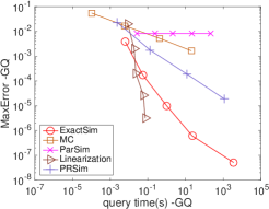
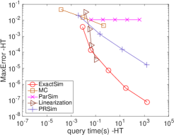
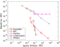
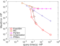
Figure 1. MaxError v.s. Query time on small graphs

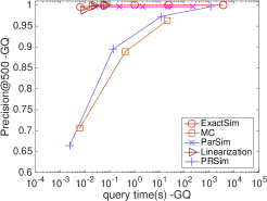
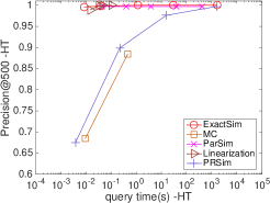
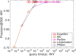
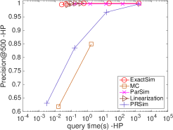
Figure 2. Precision@500 v.s. Query time on small graphs

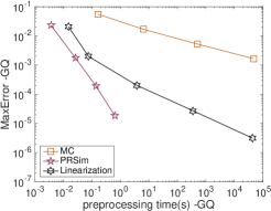
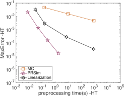
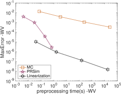
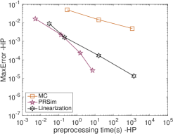
Figure 3. MaxError v.s. Preprocessing time on small graphs

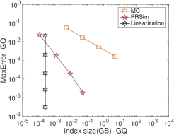
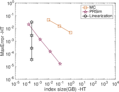
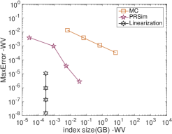
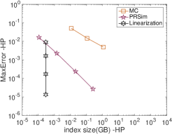
Figure 4. MaxError v.s. Index size on small graphs

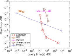
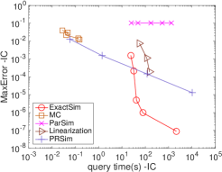
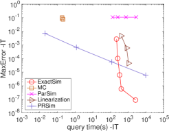
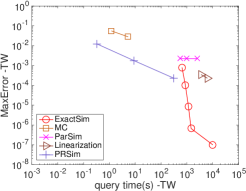
Figure 5. MaxError v.s. Query time on large graphs

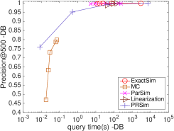
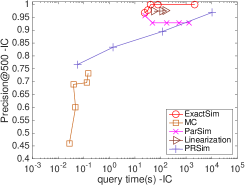
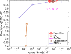
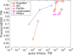
Figure 6. Precision@500 v.s. Query time on large graphs

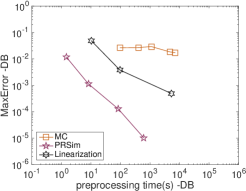
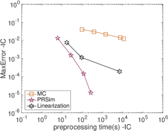
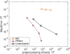
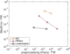
Figure 7. MaxError v.s. Preprocessing time on large graphs

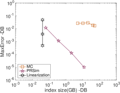
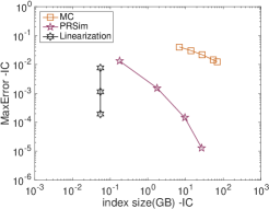
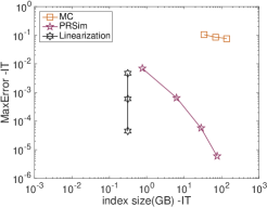
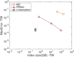
Figure 8. MaxError v.s. Index size on large graphs

Methods and Parameters. We evaluate ExactSim and other four single-source algorithms, including MC (FR05, ), Linearization (MKK14, ), ParSim (yu2015efficient, ) and PRSim (wei2019prsim, ), Among them, ExactSim, ParSim are index-free methods, and the others are index-based methods; ExactSim and ParSim can handle dynamic graphs, and the other methods can only handle static graphs. In this paper, we only focus on static graphs. For a fair comparison, we run each algorithm in the single thread mode.

MC has two parameters: the length of each random walk $L$ and the number of random walks per node $r$. We vary $(L,r)$ from $(5,50)$ to $(5000,50000)$ on small graphs and from $(5,50)$ to $(50,500)$ on large graphs. ParSim has one parameter $L$, the number of iterations. We vary it from $50$ to $5\times 10^{5}$ on small graphs and from $10$ to $500$ on large graphs. Linearization, PRSim and ExactSim share the same error parameter $\varepsilon$, and we vary $\varepsilon$ from $10^{-1}$ to $10^{-7}$ (if possible) on both small and large graphs. We evaluate the optimized ExactSim unless otherwise stated. In all experiments, we set the decay factor $c$ of SimRank as 0.6.

Metrics. We use ${MaxError}$ and Precision@k to evaluate the quality of the single-source and top-$k$ results. Given a source node $v_{i}$ and an approximate single-source result with $n$ similarities $\hat{S}(i,j),j=1,\ldots,n$, ${MaxError}$ is defined to be the maximum error over $n$ similarities: $MaxError=\max_{j=1}^{n}\left|\hat{S}(i,j)-S(i,j)\right|$. Given a source node $v_{i}$ and an approximate top-$k$ result $V_{k}=\{v_{1},\ldots,v_{k}\}$, Precision@k is defined to be the percentage of nodes in $V_{k}$ that coincides with the actual top-$k$ results. In our experiment, we set $k$ to be $500$. Note that this is the first time that top-$k$ queries with $k>100$ are evaluated on large graphs. On each dataset, we issue 50 queries and report the average ${MaxError}$ and Precision@500.

4.1. Experiments on small graphs

We first evaluate ExactSim against other single-source algorithms on four small graphs. We compute the ground truths of the single-source and top-$k$ queries using the Power Method (JW02, ). We omit a method if its query or preprocessing time exceeds $24$ hours.

Figure 1 shows the tradeoffs between ${MaxError}$ and the query time of each algorithm. The first observation is that ExactSim is the only algorithm that consistently achieves an error of $10^{-7}$ within $10^{4}$ seconds. Linearization is able to achieve a faster query time when the error parameter $\varepsilon$ is large. However, as we set $\varepsilon\leq 10^{-5}$, Linearization is troubled by its $O\left({n\log n\over\varepsilon^{2}}\right)$ preprocessing time and is unable to finish the computation of the diagonal matrix $D$ in $24$ hours.

Figure 2 presents the tradeoffs between Precision@500 and query time of each algorithm. We observe that ExactSim with $\varepsilon=10^{-7}$ is able to achieve a precision of $1$ on all four graphs. This confirms the exactness of ExactSim. We also note that ParSim is able to achieve high precisions on all four graphs despite its large ${MaxError}$ in Figure 1. This observation demonstrates the effectiveness of the $D\sim(1-c)I$ approximation on small datasets. Finally, for the index-based methods MC, PRSim and Linearization, we also plot the tradeoffs between ${MaxError}$ and preprocessing time/index size in Figure 3 and 4. The index sizes of Linearization form a vertical line, as the algorithm only recomputes and stores a diagonal matrix $D$. PRSim generally achieves the smallest error given a fixed amount of preprocessing time and index size.

4.2. Experiments on large graphs

For now, we have experimental evidence that ExactSim is able to obtain the exact single-source and top-k SimRank results on small graphs. On the other hand, the theoretical analysis in section 3 guarantees that ExactSim with $\varepsilon=10^{-7}$ can achieve a precision of 7 decimal places with high probability. Hence, we will treat the results computed by ExactSim with $\varepsilon=10^{-7}$ as the ground truths to evaluate the performance of various algorithms (including ExactSim with larger $\varepsilon$) on large graphs. We also omit a method if its query or preprocessing time exceeds 24 hours.

Figure 5 and Figure 6 show the trade-offs between the query time and ${MaxError}$ and Precision@500 of each algorithm. Figure 7 and Figure 8 display the ${MaxError}$ and preprocessing time/index size plots of the index-based algorithms. For ExactSim with $\varepsilon=10^{-7}$, we set its ${MaxError}$ as $10^{-7}$ and Precision@500 as $1$. We observe from Figure 6 that ExactSim with $\varepsilon=10^{6}$ also achieves a precision of $1$ on all four graphs. This suggests that the top-$500$ result of ExactSim with $\varepsilon=10^{-6}$ is the same as that of ExactSim with $\varepsilon=10^{-7}$. In other words, the top-$500$ result of ExactSim actually converges after $\varepsilon=10^{-6}$. This is another strong evidence of the exact nature of ExactSim. From Figure 5, We also observe that $ExactSim$ is the only algorithm that achieves an error of less than $10^{-6}$ on all four large graphs. In particular, on the TW dataset, no existing algorithm can achieve an error of less than $10^{-4}$, while ExactSim is able to achieve exactness within $10^{4}$ seconds.

4.3. Ablation study.

We now evaluate the effectiveness of the optimization techniques. Recall that we use sampling according to $\vec{\pi}_{i}(k)^{2}$ and local deterministic exploitation to reduce the query time, and sparse Linearization to reduce the space overhead. Figure 9 shows the time/error tradeoffs of the basic ExactSim and the optimized ExactSim algorithms. Under similar actual error, we observe a speedup of $10-100$ times. Table 3 shows the memory overhead of the basic ExactSim and the optimized ExactSim algorithms. We observe that the space overhead of the basic ExactSim algorithm is usually larger than the graph size, while sparse Linearization reduces the memory usage by a factor of $5-6$ times. This demonstrates the effectiveness of our optimizing techniques.

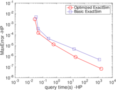
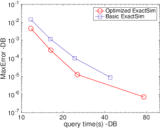
Figure 9. Basic ExactSim v.s. Optimized ExactSim

Table 3. Memory overhead on large graphs.

Memory overhead (GB)	DB	IC	IT	TW
Basic ExactSim	2.49	3.40	18.95	19.12
ExactSim	0.47	0.58	3.26	3.54
Graph size (GB)	0.48	1.88	10.94	13.30

5. Conclusions

This paper presents ExactSim, an algorithm that produces the ground truths for single-source and top-$k$ SimRank queries with precision up to 7 decimal places on large graphs. We also design various optimization techniques to improve the space and time complexity of the proposed algorithm. We believe the ExactSim algorithm can be used to produce the ground truths for evaluating single-source SimRank algorithms on large graphs. For future work, we note that the $O\left({\log n\over\varepsilon^{2}}\right)$ complexity of ExactSim prevents it from achieving a precision of $10^{-14}$ (i.e., the precision of the double type). To achieve such extreme precision, we need an algorithm with $O\left({\log n\over\varepsilon}\right)$ complexity, which remains a major open problem in SimRank study.

6. ACKNOWLEDGEMENTS

This research was supported in part by National Natural Science Foundation of China (No. 61832017, No. 61972401, No. 61932001, No. U1711261, No. 61932004 and No. 61622202), by FRFCU No. N181605012, by Beijing Outstanding Young Scientist Program NO. BJJWZYJH012019100020098, and by the Fundamental Research Funds for the Central Universities and the Research Funds of Renmin University of China under Grant 18XNLG21.

Appendix A Inequalities

A.1. Bernstein Inequality

Lemma 0 (Bernstein inequality (ChungL06, )).

Let $X_{1},\cdots,X_{R}$ be independent random variables with $|X_{i}|<b$ for $i=1,\ldots,R$. Let $X=\frac{1}{R}\cdot\sum^{R}_{i=1}X_{i}$, we have

(14) $$\Pr[|X-\mathrm{E}[X]|\geq\lambda]\leq 2\cdot\exp\left(-\frac{\lambda^{2}\cdot R}{2R\cdot\mathrm{Var}[X]+2b\lambda/3}\right),$$

where $\mathrm{Var}[X]$ is the variance of $X$.

Appendix B Proofs

B.1. Proof of Lemma 2

Proof of Lemma 2.

Note that $\hat{D}_{r}(k,k)$ is a Bernoulli random variable with expectation $D(k,k)$, and thus has variance $\mathrm{Var}[\hat{D}_{r}(k,k)]=D(k,k)(1-D(k,k))\leq D(k,k)$. Since $\hat{D}_{r}(k,k)$’s are independent random variables, we have

$$\mathrm{Var}[\vec{s}^{L}(j)]$$

$$={1\over(1-\sqrt{c})^{4}R^{2}}\sum_{k=1}^{n}\sum_{r=1}^{R\rho(k)}\left({\sum_{\ell=0}^{L}\vec{\pi}_{i}^{\ell}(k)\cdot\vec{\pi}_{j}^{\ell}(k)\over\rho(k)}\right)^{2}\cdot{\mathrm{Var}[\hat{D}_{r}(k,k)]}$$

$$={1\over(1-\sqrt{c})^{4}R}\sum_{k=1}^{n}{\left(\sum_{\ell=0}^{L}\vec{\pi}_{i}^{\ell}(k)\cdot\vec{\pi}_{j}^{\ell}(k)\right)^{2}\over\rho(k)}\cdot{D(k,k)(1-D(k,k))}.$$

By the Cauchy-Schwarz inequality, we have

$$\left(\sum_{\ell=0}^{L}\vec{\pi}_{i}^{\ell}(k)\cdot\vec{\pi}_{j}^{\ell}(k)\right)^{2} \leq\left(\sum_{\ell=0}^{L}\vec{\pi}_{i}^{\ell}(k)\right)^{2}\left(\sum_{\ell=0}^{L}\vec{\pi}_{j}^{\ell}(k)\right)^{2}$$

$$\leq\vec{\pi}_{i}(k)^{2}\vec{\pi}_{j}(k)^{2}.$$

Combining with the fact that $1-D(k,k)\leq 1$, we have

(15) $$\mathrm{Var}[\vec{s}^{L}(j)]\leq{1\over(1-\sqrt{c})^{4}R}\sum_{k=1}^{n}{\vec{\pi}_{i}(k)^{2}\vec{\pi}_{j}(k)^{2}\over\rho(k)}\cdot{D(k,k)}.$$

and the first part of the Lemma follows.

Plugging $\rho(k)=R(k)/R=\lceil R\vec{\pi}_{i}(k)\rceil/R\geq\vec{\pi}_{i}(k)$ into Lemma 2, we have

$$\mathrm{Var}[\vec{s}^{L}(j)] \leq{1\over(1-\sqrt{c})^{4}R}\sum_{k=1}^{n}{\vec{\pi}_{i}(k)^{2}\vec{\pi}_{j}(k)^{2}\over\vec{\pi}_{i}(k)}\cdot{D(k,k)}$$

$$\leq{1\over(1-\sqrt{c})^{4}R}\sum_{k=1}^{n}{\vec{\pi}_{i}(k)}.$$

For the last inequality, we use the fact that $D(k,k)\leq 1$ and $\vec{\pi}_{j}(k)\leq 1$. Finally, since $\sum_{k=1}^{n}{\vec{\pi}_{i}(k)}=1$, we have $\mathrm{Var}[\vec{s}^{L}(j)]\leq{1\over(1-\sqrt{c})^{4}R}$, and the second part of the Lemma follows. ∎

B.2. Proof of Theorem 1

Proof.

we first note that by equation (9), $\vec{s}^{L}(j)$ can be expressed as

$$\vec{s}^{L}(j) =\vec{e}_{j}\cdot\vec{s}^{L}={1\over 1-\sqrt{c}}\vec{e}_{j}^{\top}\cdot\sum_{\ell=0}^{L}\left(\sqrt{c}P^{\top}\right)^{\ell}\hat{D}\cdot\vec{\pi}_{i}^{\ell}$$

$$={1\over(1-\sqrt{c})^{2}}\sum_{\ell=0}^{L}\left((1-\sqrt{c})\left(\sqrt{c}P\right)^{\ell}\cdot\vec{e}_{j}\right)^{\top}\cdot\hat{D}\cdot\vec{\pi}_{i}^{\ell}.$$

Since $(1-\sqrt{c})\left(\sqrt{c}P\right)^{\ell}\cdot\vec{e}_{j}=\vec{\pi}_{j}^{\ell}$, we have

(16) $$\vec{s}^{L}(j)={1\over(1-\sqrt{c})^{2}}\sum_{\ell=0}^{L}\left(\vec{\pi}_{j}^{\ell}\right)^{\top}\cdot\hat{D}\cdot\vec{\pi}_{i}^{\ell}.$$

Summing up over the diagonal elements of $D$ follows that

(17) $$\vec{s}^{L}(j)={1\over(1-\sqrt{c})^{2}}\sum_{\ell=0}^{L}\sum_{k=1}^{n}\vec{\pi}_{i}^{\ell}(k)\cdot\vec{\pi}_{j}^{\ell}(k)\cdot\hat{D}(k,k).$$

Comparing the equation (17) with the actual SimRank value $S(i,j)$ given in (wei2019prsim, ) that

(18) $$S(i,j)={1\over(1-\sqrt{c})^{2}}\sum_{\ell=0}^{\infty}\sum_{k=1}^{n}\vec{\pi}_{i}^{\ell}(k)\cdot\vec{\pi}_{j}^{\ell}(k)\cdot D(k,k).$$

we observe that there are two discrepancies: 1) The iteration number changes from $\infty$ to $L$, and 2) Estimator $\hat{D}$ replaces actual diagonal correction matrix $D$. For the first approximation, we can bound the error by $c^{L}\leq\varepsilon/2$ if ExactSim sets $L=\left\lceil\log_{1\over c}{2\over\varepsilon}\right\rceil$. Consequently, we only need to bound the error from replacing $D$ with $\hat{D}$ utilizing Bernstein inequality given in Lemma 1.

According to Bernstein inequality, we need to express $\vec{s}^{L}(j)$ as the average of independent random variables. In particular, let $\hat{D}_{r}(k,k)$, $r=1,\ldots,R(k)$ denote the $r$-th estimator of $D(k,k)$ by Algorithm 2. We observe that each $\hat{D}_{r}(k,k)$ is a Bernoulli random variable, that is, $\hat{D}_{r}(k,k)=1$ with probability $D(k,k)$ and $\hat{D}_{r}(k,k)=0$ with probability $1-D(k,k)$. We have

(19) $$\vec{s}^{L}(j) ={1\over(1-\sqrt{c})^{2}}\sum_{\ell=0}^{L}\sum_{k=1}^{n}\vec{\pi}_{i}^{\ell}(k)\cdot\vec{\pi}_{j}^{\ell}(k)\cdot{\sum_{r=1}^{R(k)}\hat{D}_{r}(k,k)\over R(k)}.$$

$$={1\over(1-\sqrt{c})^{2}}\sum_{k=1}^{n}\sum_{r=1}^{R(k)}{\sum_{\ell=0}^{L}\vec{\pi}_{i}^{\ell}(k)\cdot\vec{\pi}_{j}^{\ell}(k)\over R(k)}\cdot{\hat{D}_{r}(k,k)}.$$

Let $\rho(k)=R(k)/R$ be the fraction of pairs of $\sqrt{c}$-walks assigned to $v_{k}$, it follows that

(20) $$\vec{s}^{L}(j)={1\over R}\cdot{1\over(1-\sqrt{c})^{2}}\sum_{k=1}^{n}\sum_{r=1}^{R\rho(k)}{\sum_{\ell=0}^{L}\vec{\pi}_{i}^{\ell}(k)\cdot\vec{\pi}_{j}^{\ell}(k)\over\rho(k)}\cdot{\hat{D}_{r}(k,k)}.$$

We will treat each ${\sum_{\ell=0}^{L}\vec{\pi}_{i}^{\ell}(k)\cdot\vec{\pi}_{j}^{\ell}(k)\over\rho(k)}\cdot{\hat{D}_{r}(k,k)}$ as an independent random variable. The number of such random variables is $\sum_{k=1}^{n}R\rho(k)=R$, so we have expressed $\vec{s}^{L}(j)$ as the average of $R$ independent random variables. Lemma 2 offers the variance bound of $\vec{s}^{L}(j)$. To utilize Bernstein inequality, we also need to bound $b$, the maximum value of the random variables ${\sum_{\ell=0}^{L}\vec{\pi}_{i}^{\ell}(k)\cdot\vec{\pi}_{j}^{\ell}(k)\over\rho(k)}\cdot\hat{D}_{r}(k,k)$. We have

$${\sum_{\ell=0}^{L}\vec{\pi}_{i}^{\ell}(k)\cdot\vec{\pi}_{j}^{\ell}(k)\over\vec{\pi}_{i}(k)}\cdot\hat{D}_{r}(k,k)\leq{\sum_{\ell=0}^{L}\vec{\pi}_{i}^{\ell}(k)\over\vec{\pi}_{i}(k)}\leq{\vec{\pi}_{i}(k)\over\vec{\pi}_{i}(k)}=1.$$

Applying Bernstein inequality with $b=1$ and $\mathrm{Var}[\vec{s}^{L}(j)]\leq{1\over(1-\sqrt{c})^{4}R}$, where $R={6\log n\over(1-\sqrt{c})^{4}\varepsilon^{2}}$, we have $\Pr[|\vec{s}^{L}(j)-E[\vec{s}^{L}(j)]|>\varepsilon/2]<1/n^{3}.$ Combining with the $\varepsilon/2$ error introduced by the truncation $L$, we have $\Pr[|\vec{s}^{L}(j)-S(i,j)|>\varepsilon]<1/n^{3}.$ By union bound over all possible target nodes $j=1,\ldots,n$ and all possible source nodes $i=1,\ldots,n$, we ensure that for all $n$ possible source node and $n$ target nodes,

$$\Pr[\forall i,j,\,|\vec{s}^{L}(j)-S(i,j)|>\varepsilon]<1/n,$$

and the Theorem follows.

∎

B.3. Proof of Lemma 3

Proof.

We note that the sparse Linearization introduces an extra error of $(1-\sqrt{c})^{2}\varepsilon$ to each $\vec{\pi}_{i}^{\ell}(k)$, $k=1,\ldots,n$, $\ell=0,\ldots,\infty$. According to equation (17), the estimator $\vec{s}^{L}(j)$ can be expressed as

(21) $$\vec{s}^{L}(j)={1\over(1-\sqrt{c})^{2}}\sum_{\ell=0}^{L}\sum_{k=1}^{n}\left(\vec{\pi}_{i}^{\ell}(k)\pm(1-\sqrt{c})^{2}\varepsilon\right)\cdot\vec{\pi}_{j}^{\ell}(k)\cdot\hat{D}(k,k).$$

Thus, the error introduced by sparse Linearization can be bounded by

(22) $${1\over(1-\sqrt{c})^{2}}\sum_{\ell=0}^{\infty}\sum_{k=1}^{n}(1-\sqrt{c})^{2}\varepsilon\cdot\vec{\pi}_{j}^{\ell}(k)\cdot\hat{D}(k,k).$$

Using the facts that $\sum_{\ell=0}^{\infty}\sum_{k=1}^{n}\vec{\pi}_{j}^{\ell}(k)=1$ and $\hat{D}(k,k)\leq 1$, the above error can be bounded by ${1\over(1-\sqrt{c})^{2}}\cdot(1-\sqrt{c})^{2}\varepsilon={\varepsilon}$. ∎

B.4. Proof of Lemma 4

Proof.

Recall that $\rho(k)$ is the fraction of sample assigned to $D(k,k)$. We have $\rho(k)=\left\lceil{R\vec{\pi}_{i}(k)^{2}\over\|\vec{\pi}_{i}\|^{2}}\right\rceil/R\geq{\vec{\pi}_{i}(k)^{2}\over\|\vec{\pi}_{i}\|^{2}}$. By the inequality (10) in Lemma 2, we can bound the variance of estimator $\vec{s}^{L}(j)$ as

$$\quad\mathrm{Var}[\vec{s}^{L}(j)]\leq{1\over(1-\sqrt{c})^{4}R}\sum_{k=1}^{n}{\vec{\pi}_{i}(k)^{2}\vec{\pi}_{j}(k)^{2}\over\rho(k)}\cdot{D(k,k)}$$

$$\leq{1\over(1-\sqrt{c})^{4}R}\|\vec{\pi}_{i}\|^{2}\sum_{k=1}^{n}{\vec{\pi}_{j}(k)^{2}}={1\over(1-\sqrt{c})^{4}R}\|\vec{\pi}_{i}\|^{2}\|\vec{\pi}_{j}\|^{2}.$$

Here, we use the facts that $\|\vec{\pi}_{j}\|^{2}=\sum_{k=1}^{n}\vec{\pi}_{j}(k)^{2}$ and $D(k,k)\leq 1$. Since we need to bound the variance for all possible nodes $v_{j}$ (and hence all possible $\|\vec{\pi}_{j}\|^{2}$), we make the relaxation that $\|\vec{\pi}_{j}\|^{2}\leq\|\vec{\pi}_{j}\|_{1}^{2}=1$, where $\|\vec{\pi}_{j}\|_{1}^{2}=(\sum_{k=1}^{n}|\vec{\pi}_{j}(k)|)^{2}$. And thus $\mathrm{Var}[\vec{s}^{L}(j)]\leq{1\over(1-\sqrt{c})^{4}R}\|\vec{\pi}_{i}\|^{2}.$ This suggest that by sampling according to $\vec{\pi}_{i}(k)^{2}$, we reduce the variance of the estimators by a factor $\|\vec{\pi}_{i}\|^{2}$. Recall that the ExactSim algorithm computes the Personalized PageRank vector $\vec{\pi}_{i}$ before estimating $D$, we can obtain the value of $\|\vec{\pi}_{i}\|^{2}$ and scale $R$ down by a factor of $\|\vec{\pi}_{i}\|^{2}$. This simple modification will reduce the running time to $O\left({\|\vec{\pi}_{i}\|^{2}\log n\over\varepsilon^{2}}\right)$.

One small technical issue is that the maximum of the random variables ${\sum_{\ell=0}^{\infty}\vec{\pi}_{i}^{\ell}(k)\cdot\vec{\pi}_{j}^{\ell}(k)\over\rho(k)}\cdot{\hat{D}_{r}(k,k)}$ may gets too large as the fraction $\rho(k)$ gets too small. However, by the facts that $\rho(k)=\left\lceil{R\vec{\pi}_{i}(k)^{2}\over\|\vec{\pi}_{i}\|^{2}}\right\rceil/R$ and $\hat{D}_{r}(k,k)\leq 1$, we have

$${\sum_{\ell=0}^{\infty}\vec{\pi}_{i}^{\ell}(k)\cdot\vec{\pi}_{j}^{\ell}(k)\over\rho(k)}\cdot{\hat{D}_{r}(k,k)}\leq{\vec{\pi}_{i}(k)\over\rho(k)}=R\vec{\pi}_{i}(k)/\left\lceil{R\vec{\pi}_{i}(k)^{2}\over\|\vec{\pi}_{i}\|^{2}}\right\rceil.$$

If we view the right side of the above equality as a function of $\vec{\pi}_{i}(k)$, it takes maximum when ${R\vec{\pi}_{i}(k)^{2}\over\|\vec{\pi}_{i}\|^{2}}=1$, or equivalently $\vec{\pi}_{i}(k)=\sqrt{\|\vec{\pi}_{i}\|^{2}\over R}$. Thus, the random variables in equation (20) can be bounded by $R\sqrt{\|\vec{\pi}_{i}\|^{2}\over R}=\|\vec{\pi}_{i}\|\sqrt{R}$. Plugging $b=\|\vec{\pi}_{i}\|\sqrt{R}$ and $\mathrm{Var}[\vec{s}^{L}(j)]\leq{1\over(1-\sqrt{c})^{4}R}\|\vec{\pi}_{i}\|^{2}$ into bernstein inequality, and the Lemma follows. ∎

B.5. Proof of Lemma 5

Proof.

Note that $\left(\sqrt{c}\right)^{\ell}\left(P^{\top}\right)^{\ell}(k,q)$ is the probability that a $\sqrt{c}$-walk from $v_{k}$ visits $v_{q}$ at its $\ell$-th step. Consequently, $c^{\ell}\left(P^{\top}\right)^{\ell}(k,q)^{2}$ is the probability that two $\sqrt{c}$-walks from node $v_{k}$ visit node $v_{q}$ at their $\ell$-th step simultaneously. To ensure this is the first time that the two $\sqrt{c}$-walks meet, we subtract the probability mass that the two $\sqrt{c}$-walks have met before. In particular, recall that $Z_{\ell^{\prime}}(k,q^{\prime})$ is the probability that two $\sqrt{c}$-walks from node $v_{k}$ first meet at $v_{q^{\prime}}$ in exactly $\ell^{\prime}$ steps. Due to the memoryless property of the $\sqrt{c}$-walk, the two $\sqrt{c}$-walks will behave as two new $\sqrt{c}$-walks from $v_{q^{\prime}}$ after their $\ell^{\prime}$-th step. The probability that these two new $\sqrt{c}$-walks visitis $v_{q}$ in exact $\ell-\ell^{\prime}$ steps is $c^{\ell-\ell^{\prime}}\left(P^{\top}\right)^{\ell-\ell^{\prime}}(q^{\prime},q)^{2}$. Summing up $q^{\prime}$ from $1$ to $n$ and $\ell^{\prime}$ from $1$ to $\ell-1$, and the Lemma follows. ∎

References

- [1] http://snap.stanford.edu/data.
- [2] http://law.di.unimi.it/datasets.php.
- [3] Reid Andersen, Fan R. K. Chung, and Kevin J. Lang. Local graph partitioning using pagerank vectors. In FOCS, pages 475–486, 2006.
- [4] Ioannis Antonellis, Hector Garcia Molina, and Chi Chao Chang. Simrank++: query rewriting through link analysis of the click graph. PVLDB, 1(1):408–421, 2008.
- [5] Bahman Bahmani, Abdur Chowdhury, and Ashish Goel. Fast incremental and personalized pagerank. VLDB, 4(3):173–184, 2010.
- [6] Mansurul Bhuiyan and Mohammad Al Hasan. Representing graphs as bag of vertices and partitions for graph classification. Data Science and Engineering, 3(2):150–165, 2018.
- [7] Fan R. K. Chung and Lincoln Lu. Concentration inequalities and martingale inequalities: A survey. Internet Mathematics, 3(1):79–127, 2006.
- [8] Daniel Fogaras and Balazs Racz. Scaling link-based similarity search. In WWW, pages 641–650, 2005.
- [9] Dániel Fogaras, Balázs Rácz, Károly Csalogány, and Tamás Sarlós. Towards scaling fully personalized pagerank: Algorithms, lower bounds, and experiments. Internet Mathematics, 2(3):333–358, 2005.
- [10] Yuichiro Fujiwara, Makoto Nakatsuji, Hiroaki Shiokawa, and Makoto Onizuka. Efficient search algorithm for simrank. In ICDE, pages 589–600, 2013.
- [11] Guoming He, Haijun Feng, Cuiping Li, and Hong Chen. Parallel simrank computation on large graphs with iterative aggregation. In KDD, pages 543–552, 2010.
- [12] Glen Jeh and Jennifer Widom. Simrank: a measure of structural-context similarity. In SIGKDD, pages 538–543, 2002.
- [13] Minhao Jiang, Ada Wai-Chee Fu, and Raymond Chi-Wing Wong. Reads: a random walk approach for efficient and accurate dynamic simrank. PPVLDB, 10(9):937–948, 2017.
- [14] Mitsuru Kusumoto, Takanori Maehara, and Ken-ichi Kawarabayashi. Scalable similarity search for simrank. In SIGMOD, pages 325–336, 2014.
- [15] Pei Lee, Laks V. S. Lakshmanan, and Jeffrey Xu Yu. On top-k structural similarity search. In ICDE, pages 774–785, 2012.
- [16] Cuiping Li, Jiawei Han, Guoming He, Xin Jin, Yizhou Sun, Yintao Yu, and Tianyi Wu. Fast computation of simrank for static and dynamic information networks. In EDBT, pages 465–476, 2010.
- [17] Lina Li, Cuiping Li, Hong Chen, and Xiaoyong Du. Mapreduce-based simrank computation and its application in social recommender system. In 2013 IEEE international congress on big data, pages 133–140. IEEE, 2013.
- [18] Zhenguo Li, Yixiang Fang, Qin Liu, Jiefeng Cheng, Reynold Cheng, and John Lui. Walking in the cloud: Parallel simrank at scale. PVLDB, 9(1):24–35, 2015.
- [19] Zhenjiang Lin, Michael R Lyu, and Irwin King. Matchsim: a novel similarity measure based on maximum neighborhood matching. KAIS, 32(1):141–166, 2012.
- [20] Yu Liu, Bolong Zheng, Xiaodong He, Zhewei Wei, Xiaokui Xiao, Kai Zheng, and Jiaheng Lu. Probesim: scalable single-source and top-k simrank computations on dynamic graphs. PVLDB, 11(1):14–26, 2017.
- [21] Dmitry Lizorkin, Pavel Velikhov, Maxim Grinev, and Denis Turdakov. Accuracy estimate and optimization techniques for simrank computation. The VLDB Journal, 19(1):45–66, 2010.
- [22] Dmitry Lizorkin, Pavel Velikhov, Maxim N. Grinev, and Denis Turdakov. Accuracy estimate and optimization techniques for simrank computation. VLDB J., 19(1):45–66, 2010.
- [23] Linyuan Lü and Tao Zhou. Link prediction in complex networks: A survey. Physica A: statistical mechanics and its applications, 390(6):1150–1170, 2011.
- [24] Takanori Maehara, Mitsuru Kusumoto, and Ken-ichi Kawarabayashi. Efficient simrank computation via linearization. CoRR, abs/1411.7228, 2014.
- [25] Takanori Maehara, Mitsuru Kusumoto, and Ken-ichi Kawarabayashi. Scalable simrank join algorithm. In ICDE, pages 603–614, 2015.
- [26] Lawrence Page, Sergey Brin, Rajeev Motwani, and Terry Winograd. The pagerank citation ranking: bringing order to the web. 1999.
- [27] Yingxia Shao, Bin Cui, Lei Chen, Mingming Liu, and Xing Xie. An efficient similarity search framework for simrank over large dynamic graphs. PVLDB, 8(8):838–849, 2015.
- [28] Wenbo Tao, Minghe Yu, and Guoliang Li. Efficient top-k simrank-based similarity join. PVLDB, 8(3):317–328, 2014.
- [29] Boyu Tian and Xiaokui Xiao. SLING: A near-optimal index structure for simrank. In SIGMOD, pages 1859–1874, 2016.
- [30] Anton Tsitsulin, Davide Mottin, Panagiotis Karras, and Emmanuel Müller. Verse: Versatile graph embeddings from similarity measures. In WWW, pages 539–548. International World Wide Web Conferences Steering Committee, 2018.
- [31] Zhewei Wei, Xiaodong He, Xiaokui Xiao, Sibo Wang, Yu Liu, Xiaoyong Du, and Ji-Rong Wen. Prsim: Sublinear time simrank computation on large power-law graphs. In SIGMOD, pages 1042–1059. ACM, 2019.
- [32] Wensi Xi, Edward A Fox, Weiguo Fan, Benyu Zhang, Zheng Chen, Jun Yan, and Dong Zhuang. Simfusion: measuring similarity using unified relationship matrix. In SIGIR, pages 130–137. ACM, 2005.
- [33] Qi Ye, Changlei Zhu, Gang Li, Zhimin Liu, and Feng Wang. Using node identifiers and community prior for graph-based classification. Data Science and Engineering, 3(1):68–83, 2018.
- [34] Weiren Yu, Xuemin Lin, and Wenjie Zhang. Fast incremental simrank on link-evolving graphs. In ICDE, pages 304–315, 2014.
- [35] Weiren Yu, Xuemin Lin, Wenjie Zhang, Lijun Chang, and Jian Pei. More is simpler: Effectively and efficiently assessing node-pair similarities based on hyperlinks. PVLDB, 7(1):13–24, 2013.
- [36] Weiren Yu and Julie McCann. Gauging correct relative rankings for similarity search. In CIKM, pages 1791–1794, 2015.
- [37] Weiren Yu and Julie A. McCann. Efficient partial-pairs simrank search for large networks. PVLDB, 8(5):569–580, 2015.
- [38] Weiren Yu and Julie A McCann. Efficient partial-pairs simrank search on large networks. Proceedings of the VLDB Endowment, 8(5):569–580, 2015.
- [39] Weiren Yu and Julie Ann McCann. High quality graph-based similarity search. In SIGIR, pages 83–92, 2015.
- [40] Weiren Yu, Wenjie Zhang, Xuemin Lin, Qing Zhang, and Jiajin Le. A space and time efficient algorithm for simrank computation. World Wide Web, 15(3):327–353, 2012.
- [41] Jing Zhang, Jie Tang, Cong Ma, Hanghang Tong, Yu Jing, and Juanzi Li. Panther: Fast top-k similarity search on large networks. In SIGKDD, pages 1445–1454. ACM, 2015.
- [42] Peixiang Zhao, Jiawei Han, and Yizhou Sun. P-rank: a comprehensive structural similarity measure over information networks. In CIKM, pages 553–562. ACM, 2009.
- [43] Peixiang Zhao, Jiawei Han, and Yizhou Sun. P-rank: a comprehensive structural similarity measure over information networks. In CIKM, pages 553–562, 2009.
- [44] Weiguo Zheng, Lei Zou, Yansong Feng, Lei Chen, and Dongyan Zhao. Efficient simrank-based similarity join over large graphs. PVLDB, 6(7):493–504, 2013.