Inference in Unbalanced Panel Data Models with Interactive Fixed Effects

In this article, we study the limiting behavior of [7]’s interactive fixed effects estimator in the presence of randomly missing data. In extensive simulation experiments, we show that the inferential theory derived by b2009mw2017 approximates the behavior of the estimator fairly well. However, we find that the fraction and pattern of randomly missing data affect the performance of the estimator. Additionally, we use the interactive fixed effects estimator to reassess the baseline analysis of [1]. Allowing for a more general form of unobserved heterogeneity as the authors, we confirm significant effects of democratization on growth. JEL Classification: C01, C13, C23, C38, C55, O10
Keywords: Economic Development, Interactive Fixed Effects, Factor Models, Model Selection, Principal Components, Unbalanced Panel Data

Introduction

Economists are often concerned that unobserved heterogeneity is correlated with some variables of interest and thus leads to inconsistent estimates of the corresponding common parameters $\boldsymbol{\beta}$. If panel data is available, so called fixed effects models are frequently used to address this issue. One critical assumption of these models is that the unobserved heterogeneity has to be additive separable in both panel dimensions. For instance, if a panel consists of $N$ individuals observed for $T$ time periods, the researcher has to assume that individual- and/or time-specific effects enter the model additively. If this is not the case, for instance because both effects are multiplicatively interacted, conventional fixed effects models are not suitable to solve the underlying endogeneity problem. Exactly this concern motivates so-called interactive fixed effects (IFE) estimators that model the time-varying unobserved heterogeneity as a low rank factor structure $\boldsymbol{\lambda}_{i}^{\prime}\mathbf{f}_{t}^{\phantom{\prime}}$, where $\boldsymbol{\lambda}_{i}$ and $\mathbf{f}_{t}$ are individual- and time-specific effects, respectively (see among others hnr1988p2006b2009). Throughout this article, we refer to $\boldsymbol{\lambda}_{i}$ as factor loadings and $\mathbf{f}_{t}$ as common factors.

[34] propose an estimator for panels with large $N$ but small $T$ which is based on a quasi-differencing approach similar to [4]. First they eliminate the factor loadings from the estimation equation and then estimate the remaining common factors and parameters using lagged covariates as instrumental variables. Although this estimator is consistent under fixed $T$ asymptotics, its is well known that for large $T$, the number of instruments and parameters leads to biased estimates (see [41]). Recently, the literature considers estimators that require $N$ and $T$ to be sufficiently large. [46] suggests a common correlated effects (CEE) estimator in the spirit of m1978c1982c1984, which uses cross-sectional averages of the dependent variable and the regressors to control for the unobserved common factors. His estimator is at least $\sqrt{N}$ consistent without the need to know the true rank of the factor structure or to impose strong factor assumptions as in b2009mw2015mw2017. However, in order to use cross-sectional averages as proxy variables for the unobserved common factors, we require some parametric assumptions on the joint probability distributions of the dependent variable and the covariates. [7] suggests a different estimator that treats the common factors and factor loadings as nuisance parameters to be estimated. His estimator is closely related to [6]’s principal components estimator for pure factor models and has the advantage that we do not need to make distributional assumptions about unobserved heterogeneity and that we allow for arbitrary correlations with the variables of interest. Under the assumption that the true number of factors is known, [7] shows $\sqrt{NT}$ consistency irrespective of cross-sectional and/or time-serial dependence in the idiosyncratic error term. However, the presence of cross-sectional and/or time-serial dependence leads to an asymptotic bias in the limiting distribution of the estimator that can be corrected (see [7]). [38] derived an additional bias correction for the [44] bias stemming from the inclusion of predetermined and weakly exogenous regressors. Because the true number of factors is usually unknown, [37] show that under certain assumptions and as long as the number of factors used to estimate $\boldsymbol{\beta}$ is larger than the true number, the estimator may have the same limiting distribution as shown by [7] but remains at least $\sqrt{\min(N,T)}$ consistent. There may therefore be a loss of efficiency due to the inclusion of too many irrelevant factors. However, given a consistent estimator for $\boldsymbol{\beta}$, the number of factors can be estimated using estimators for pure factor models (see among others be1992bn2002hl2007abc2010o2010ah2013do2019). A recent comparison of some popular estimators is given in [22]. For the IFE estimator such a comparison does not exist so far.

Additionally, it is often the case that some of the observations in a panel are missing. One frequent reason is attrition. For instance, some individuals drop out of a panel because they move or leave the participating household. In some of these cases, those individuals are replaced. In macroeconomic panels, it also occurs that some countries are divided into several independent countries. Further, some survey designs replace individuals because of non-response. All these cases lead to very different patterns of missing data that usually, in the absence of sample selection, do not affect the properties of the estimators (see [26]). However in the presence of missing data, the principal component estimator of [7] requires an additional data augmentation step based on the EM algorithm of sw1998sw2002 (see Appendix of [7] and [9]). [9] show consistency of the EM-type estimator in extensive simulation studies, but do not further investigate the limiting behavior of the estimator.

Our article makes the following contributions. First, we extend the work of [9] and show that the limiting behavior of their suggested estimator can be fairly well approximated by the inferential theory of b2009mw2017 derived for balanced panels. In extensive simulation experiments, we show that the fraction and pattern of missing data may affect the properties of the estimator, which is contrary to other popular unobserved effects estimators like the conventional within estimator (see [26]). Further, we present some algorithms that reduce the computational costs in the presence of missing data. Second, because the limiting theory of b2009mw2017 assumes that the true number of factors is known, we additionally investigate the finite sample performance of some frequently used estimators for the number of factors: bn2002o2010ah2013do2019. Although we find that all estimators perform well for balanced data and different configurations of the idiosyncratic error term, their accuracy varies substantially with different fractions and patterns of randomly missing data. Third, we contribute to the literature of growth by reassessing the baseline analysis of [1] using the IFE estimator of [7]. We qualitatively confirm their main results and find significant effects of democratization on growth. In their preferred specification, we estimate a long-run effect of 18 %, which is pretty close to the 20 % reported by the authors, but the instantaneous effect of democratization almost halves to 0.6 %.

The article is organized as follows. We introduce the model and the corresponding estimator in Section 2. We briefly review some estimators for the number of factors in Section 3. We provide results of extensive simulation experiments in Section 4. We reassess [1] using the IFE estimator in Section 5. We briefly discuss the handling of endogenous regressors as in mw2017msw2018 and consider an alternative estimator suggested by [39] in Section 6. Finally, we conclude in Section 7.

Throughout this article, we follow conventional notation: scalars are represented in standard type, vectors and matrices in boldface, and all vectors are column vectors. Further, let $\mathbf{A}$ be a $N\times N$ matrix and $\mathbf{B}$ be a $N\times T$ matrix. We denote $\mu_{r}[\mathbf{A}]$ as the $r$-th largest eigenvalue of $\mathbf{A}$, we refer to $[\mathbf{B}]_{ij}$ as the $ij$-th element of $\mathbf{B}$, and we define $\operatorname{\mathbb{M}}_{\mathbf{B}}=\operatorname{\mathbf{1}}_{N}-\operatorname{\mathbb{P}}_{\mathbf{B}}$, where $\operatorname{\mathbf{1}}_{N}$ is a $N\times N$ identity matrix, $\operatorname{\mathbb{P}}_{\mathbf{B}}=\mathbf{B}(\mathbf{B}^{\prime}\mathbf{B})^{\dagger}\mathbf{B}^{\prime}$, and $(\cdot)^{\dagger}$ is the Moore-Penrose pseudoinverse.

Model and Estimation

Model, Consistency, and Asymptotic Distribution

In this article, we analyze the following unobserved effects model:

$$y_{it}=\mathbf{x}_{it}^{\prime}\boldsymbol{\beta}+\boldsymbol{\lambda}_{i}^{\prime}\mathbf{f}_{t}^{\phantom{\prime}}+e_{it}\,,$$ (1)

where $i$ and $t$ are individual and time specific indexes, $\mathbf{x}_{it}=[x_{it,1},\ldots,x_{it,K}]^{\prime}$ is a vector of $K$ explanatory variables, $\boldsymbol{\beta}$ is the corresponding vector of common parameters, and $e_{it}$ is an idiosyncratic error term. To allow for the possibility of missing data, we introduce $\mathcal{D}$ as a subset of observed index pairs such that $\mathcal{D}\subseteq\{(i,t)|i\in\{1,\ldots,N\}\wedge t\in\{1,\ldots,T\}\}$, where $n=\lvert\mathcal{D}\rvert$ is the sample size and $N$ and $T$ are the number of individuals and time periods, respectively. Further, the unobserved effects are expressed as a factor structure of rank $R\ll\min(N,T)$, where $\boldsymbol{\lambda}_{i}=[\lambda_{i1},\ldots,\lambda_{iR}]^{\prime}$ is a vector of factor loadings and $\mathbf{f}_{t}=[f_{t1},\ldots,f_{tR}]^{\prime}$ is a vector of common factors. Note that (1) collapses to the conventional additive unobserved effects model if $\boldsymbol{\lambda}_{i}=[\alpha_{i},1]^{\prime}$ and $\mathbf{f}_{t}=[1,\delta_{t}]^{\prime}$. In contrast to this conventional model, the factor structure allows to capture more general patterns of heterogeneity. For instance, temporal shocks induced by financial crises might differently affect each countries output (see [7] for some additional motivating examples).

Following b2009mw2017, we treat $\boldsymbol{\lambda}_{i}$ and $\mathbf{f}_{t}$ as parameters to be estimated, and allow the common factors and loadings to be arbitrarily related with the regressors. To stress the similarity with the conventional fixed effects model, we follow the existing literature and refer to (1) as interactive fixed effects model.

For a given value of $R$, mw2015mw2017 suggest

$$\hat{\boldsymbol{\beta}}=\underset{\boldsymbol{\beta}\in\mathbb{R}^{K}}{\operatorname{\arg\,\min\;}}Q\left(\boldsymbol{\beta}\right)$$ (2)

as IFE estimator for $\boldsymbol{\beta}$, where

$$Q\left(\boldsymbol{\beta}\right)=\underset{\boldsymbol{\Lambda},\mathbf{F}}{\min}\;\frac{1}{n}\sum_{(i,t)\in\mathcal{D}}\left(y_{it}-\mathbf{x}_{it}^{\prime}\boldsymbol{\beta}-\boldsymbol{\lambda}_{i}^{\prime}\mathbf{f}_{t}^{\phantom{\prime}}\right)^{2}$$ (3)

is the profile objective function, $\boldsymbol{\Lambda}=[\boldsymbol{\lambda}_{1},\ldots,\boldsymbol{\lambda}_{N}]^{\prime}$ is a $N\times R$ matrix of factor loadings, and $\mathbf{F}=[\mathbf{f}_{1},\ldots,\mathbf{f}_{T}]^{\prime}$ is a $T\times R$ matrix of common factors. Note that the minimizing common factors $\hat{\mathbf{f}}_{t}(\boldsymbol{\beta})$ and loadings $\hat{\boldsymbol{\lambda}}_{i}(\boldsymbol{\beta})$ are not uniquely determined without imposing further normalizing restrictions. However, their column spaces are, which means their product is unique. We will return to this issue in the next subsection. Further, the objective function is globally non-convex due to the rank constraint imposed on the factor structure.

[38] show consistency of the IFE estimator using an asymptotic framework where $N,T\rightarrow\infty$. Most notably, their imposed assumptions require the true number of factors to be known, some regularity assumptions, weak exogeneity of the regressors, and some conditions with respect to so called “low-rank” regressors. The latter assumptions ensure that these “low-rank” regressors are not entirely absorbed by the factor structure, which otherwise leads to an identification problem. This is very similar to the conventional fixed effects model where coefficients of time-invariant regressors are not identified. Note that [7] also shows consistency using different asymptotics that requires strict exogeneity of all regressors. However, his framework is not suitable for our purposes because we will consider predetermined regressors in our empirical illustration.

We briefly describe the asymptotic distribution of the IFE estimator derived by [38] and adjust it using the conjecture of [26] for randomly missing data. To avoid ambiguity, by randomly missing observations, we mean that the dependent variable is independent of the attrition process conditional on the covariates and factor structure. Thus we assume that the observations are conditionally missing at random. Under asymptotic sequences where $N/T\rightarrow\kappa^{2}$ and $0<\kappa<\infty$, the IFE estimator has the following limiting distribution:

$$\hat{\boldsymbol{\beta}}\overset{d}{\rightarrow}\operatorname{\mathcal{N}}\left(\boldsymbol{\beta}-\overline{N}^{-1}\mathbf{B}-\overline{T}^{-1}\mathbf{C}_{1}-\overline{T}^{-1}\mathbf{C}_{2},n^{-1}\mathbf{V}\right)\,,$$ (4)

where $\overline{N}=n/T$, $\overline{T}=n/N$, $\mathbf{B}$, $\mathbf{C}_{1}$, and $\mathbf{C}_{2}$ are leading bias terms, and $\mathbf{V}$ is a covariance matrix. $\mathbf{C}_{1}$ stems from the inclusion of weakly exogenous regressors, like predetermined variables, and is a generalization of the [44] bias. $\mathbf{B}$ and $\mathbf{C}_{2}$ arise if the idiosyncratic error term is heteroskedastic or correlated across individuals and time periods, respectively.

Estimation Algorithm

[38] show that (3) can be transformed to

$$Q\left(\boldsymbol{\beta}\right)=\frac{1}{n}\sum_{r=R+1}^{\min(N,T)}\mu_{r}\left[\mathbf{W}\left(\boldsymbol{\beta}\right)^{\prime}\mathbf{W}\left(\boldsymbol{\beta}\right)\right]\,,$$ (5)

where $\mathbf{W}(\boldsymbol{\beta})$ is a $N\times T$ matrix with $[\mathbf{W}(\boldsymbol{\beta})]_{it}=y_{it}-\mathbf{x}_{it}^{\prime}\boldsymbol{\beta}$. However, in the presence of missing data, some of the entries in $\mathbf{W}(\boldsymbol{\beta})$ are missing and we cannot simply apply the eigendecomposition as in the balanced case.

We follow the suggestion of b2009bly2015 and combine (5) with an EM algorithm proposed by sw1998sw2002. Intuitively, we augment the missing data in the E-step and apply the eigendecomposition to complete data in the M-step. Following [9], we can rearrange (1) to

$$y_{it}-\mathbf{x}_{it}^{\prime}\boldsymbol{\beta}=\left[\mathbf{W}\left(\boldsymbol{\beta}\right)\right]_{it}=\boldsymbol{\lambda}_{i}^{\prime}\mathbf{f}_{t}^{\phantom{\prime}}+e_{it}\,,$$ (6)

which means that, for a known $\boldsymbol{\beta}$, we can augment missing observations in $\mathbf{W}(\boldsymbol{\beta})$ with estimates of $\boldsymbol{\Lambda}$ and $\mathbf{F}$. As [7], we impose the following normalizing restrictions to uniquely determine the common factors and loadings: $\mathbf{F}^{\prime}\mathbf{F}^{\phantom{\prime}}/T=\operatorname{\mathbf{1}}_{R}$ and $\boldsymbol{\Lambda}^{\prime}\boldsymbol{\Lambda}^{\phantom{\prime}}=\operatorname{\text{diag}\;}(\boldsymbol{\alpha})$, where $\boldsymbol{\alpha}\in\mathbb{R}^{R}$. Given these normalizing restrictions, $\widehat{\mathbf{F}}(\boldsymbol{\beta})$ is equal to the first $R$ eigenvectors of $\mathbf{W}(\boldsymbol{\beta})^{\prime}\mathbf{W}(\boldsymbol{\beta})$ multiplied by $\sqrt{T}$ and $\widehat{\boldsymbol{\Lambda}}(\boldsymbol{\beta})=\mathbf{W}(\boldsymbol{\beta})\widehat{\mathbf{F}}(\boldsymbol{\beta})/T$.

Before we describe the entire EM algorithm, we introduce some additional notation. Let

$$\left[\mathfrak{P}_{\mathcal{D}}^{\phantom{\perp}}\left(\mathbf{A}\right)\right]_{it}=\begin{cases}\left[\mathbf{A}\right]_{it}&\text{if}\;\;(i,t)\in\mathcal{D}\\ 0&\text{otherwise}\end{cases}$$ (7)

be a projection operator that replaces missing observations of any $N\times T$ matrix $\mathbf{A}$ with zeros. Likewise, $\mathfrak{P}_{\mathcal{D}}^{\perp}(\mathbf{A})$ is the complementary operator that replaces non-missing observations with zeros.

Definition.

EM algorithm

Given $\boldsymbol{\beta}$ and $R$, initialize $\mathbf{W}^{\perp}=\mathbf{0}_{N\times T}$ and repeat the following steps until convergence

• Set $\widetilde{\mathbf{W}}\left(\boldsymbol{\beta}\right)=\mathfrak{P}_{\mathcal{D}}^{\phantom{\perp}}\left(\mathbf{W}\left(\boldsymbol{\beta}\right)\right)+\mathfrak{P}_{\mathcal{D}}^{\perp}\left(\mathbf{W}^{\perp}\right)$

• Compute $\widehat{\mathbf{F}}\left(\boldsymbol{\beta}\right)$ and $\widehat{\boldsymbol{\Lambda}}\left(\boldsymbol{\beta}\right)$ from $\widetilde{\mathbf{W}}\left(\boldsymbol{\beta}\right)$

• Update $\mathbf{W}^{\perp}=\widehat{\boldsymbol{\Lambda}}\left(\boldsymbol{\beta}\right)\widehat{\mathbf{F}}\left(\boldsymbol{\beta}\right)^{\prime}$

For a given $\boldsymbol{\beta}$ and $R$, we start by replacing missing observations in $\mathbf{W}(\boldsymbol{\beta})$ with zeros. We denote this augmented matrix as $\widetilde{\mathbf{W}}(\boldsymbol{\beta})$. Afterwards we estimate $\widehat{\mathbf{F}}(\boldsymbol{\beta})$ and $\widehat{\boldsymbol{\Lambda}}(\boldsymbol{\beta})$ from $\widetilde{\mathbf{W}}(\boldsymbol{\beta})$, replace the missing observations in $\widetilde{\mathbf{W}}(\boldsymbol{\beta})$ with $\hat{\boldsymbol{\lambda}}_{i}^{\prime}(\boldsymbol{\beta})\,\hat{\mathbf{f}}_{t}^{\phantom{\prime}}(\boldsymbol{\beta})$, and repeat these two steps until convergence.

Let $\widetilde{\mathbf{W}}(\boldsymbol{\beta})$ denote the augmented matrix after convergence, a general IFE objective function is given by

$$\widetilde{Q}\left(\boldsymbol{\beta}\right)=\frac{1}{n}\sum_{r=R+1}^{\min(N,T)}\mu_{r}\left[\widetilde{\mathbf{W}}\left(\boldsymbol{\beta}\right)^{\prime}\widetilde{\mathbf{W}}\left(\boldsymbol{\beta}\right)\right]\,,$$ (8)

where in case of balanced data $\widetilde{\mathbf{W}}(\boldsymbol{\beta})$ is simply $\mathbf{W}(\boldsymbol{\beta})$. Thus, in case of missing data, we complement the IFE estimator suggested by mw2015mw2017 with an additional data augmentation step inside the objective function.

Bias Correction and Inference

Before we describe the estimation of the leading bias terms and the covariance matrix necessary for inference, we need to know how to project the estimated common factors and/or loadings out of an arbitrary $n$-dimensional vector $\mathbf{v}$. Let $\breve{\mathbf{v}}$, $\grave{\mathbf{v}}$, and $\acute{\mathbf{v}}$ denote the residuals of the following least squares problems:

$$\breve{v}_{it}= v_{it}-\hat{\boldsymbol{\lambda}}_{i}^{\prime}\hat{\mathbf{a}}_{t}^{\phantom{\prime}}-\hat{\mathbf{f}}_{t}^{\prime}\hat{\mathbf{b}}_{i}^{\phantom{\prime}}\,, \left(\widehat{\mathbf{A}},\widehat{\mathbf{B}}\right)= \underset{\mathbf{A}\in\mathbb{R}^{T\times R},\,\mathbf{B}\in\mathbb{R}^{N\times R}}{\operatorname{\arg\,\min\;}}\sum_{(i,t)\in\mathcal{D}}\left(v_{it}-\hat{\boldsymbol{\lambda}}_{i}^{\prime}\mathbf{a}_{t}^{\phantom{\prime}}-\hat{\mathbf{f}}_{t}^{\prime}\mathbf{b}_{i}^{\phantom{\prime}}\right)^{2}\,,$$ (9)

$$\grave{v}_{it}= v_{it}-\hat{\boldsymbol{\lambda}}_{i}^{\prime}\hat{\mathbf{a}}_{t}^{\phantom{\prime}}\,, \widehat{\mathbf{A}}= \quad\underset{\mathbf{A}\in\mathbb{R}^{T\times R}}{\operatorname{\arg\,\min\;}}\sum_{(i,t)\in\mathcal{D}}\left(v_{it}-\hat{\boldsymbol{\lambda}}_{i}^{\prime}\mathbf{a}_{t}^{\phantom{\prime}}\right)^{2}\,,$$ (10)

$$\acute{v}_{it}= v_{it}-\hat{\mathbf{f}}_{t}^{\prime}\hat{\mathbf{b}}_{i}^{\phantom{\prime}}\,, \widehat{\mathbf{B}}= \quad\underset{\mathbf{B}\in\mathbb{R}^{N\times R}}{\operatorname{\arg\,\min\;}}\sum_{(i,t)\in\mathcal{D}}\left(v_{it}-\hat{\mathbf{f}}_{t}^{\prime}\mathbf{b}_{i}^{\phantom{\prime}}\right)^{2}\,,$$ (11)

where $\mathbf{A}=[\mathbf{a}_{1},\ldots,\mathbf{a}_{T}]^{\prime}$ and $\mathbf{B}=[\mathbf{b}_{1},\ldots,\mathbf{b}_{N}]^{\prime}$. In case of balanced data, these residuals have a straightforward expression: $\breve{\mathbf{v}}=\operatorname{\text{vec}\;}(\operatorname{\mathbb{M}}_{\widehat{\boldsymbol{\Lambda}}}\mathbf{V}\operatorname{\mathbb{M}}_{\widehat{\mathbf{F}}})$, $\grave{\mathbf{v}}=\operatorname{\text{vec}\;}(\operatorname{\mathbb{M}}_{\widehat{\boldsymbol{\Lambda}}}\mathbf{V})$, and $\acute{\mathbf{v}}=\operatorname{\text{vec}\;}(\mathbf{V}\operatorname{\mathbb{M}}_{\widehat{\mathbf{F}}})$, where $\mathbf{V}$ is a $N\times T$ matrix with elements denoted by $v_{it}$. However in the presence of missing data, we cannot simply augment missing observations in $\mathbf{V}$ with zeros and apply the same expressions as in the balanced case. We can still use a standard ordinary least squares estimator to obtain the residuals, but with increasing sample sizes this problem quickly becomes infeasible (even for moderately large data sets). Suppose we have a data set consisting of $N=200$ individuals observed for $T=50$ time periods and consider five factors. Even in this moderate example, the rank of the sparse regressor matrix corresponding to the common factors and factor loadings is already $(N+T)\,R=1,250$. Fortunately, we can use insights from the literature about conventional fixed effects models and use sparse solvers like h1962fs2011 to mitigate this problem (see gp2010g2013s2018).

In the presence of missing data, we recommend to compute the residuals with the method of alternating projections (MAP, see [33]) approach suggested by [49]. Let $\mathcal{D}_{t}=\{i\mid(i,t)\in\mathcal{D}\}$ and $\mathcal{D}_{i}=\{t\mid(i,t)\in\mathcal{D}\}$, we define the following scalar expressions:

$$\left[\mathbf{M}_{\hat{\boldsymbol{\lambda}}_{r}}\mathbf{v}\right]_{it}=v_{it}-\hat{\lambda}_{ir}\frac{\sum_{i\in\mathcal{D}_{t}}\hat{\lambda}_{ir}v_{it}}{\sum_{i\in\mathcal{D}_{t}}\hat{\lambda}_{ir}^{2}}\quad\text{and}\quad\left[\mathbf{M}_{\hat{\mathbf{f}}_{r}}\mathbf{v}\right]_{it}=v_{it}-\hat{f}_{tr}\frac{\sum_{t\in\mathcal{D}_{i}}\hat{f}_{tr}v_{it}}{\sum_{t\in\mathcal{D}_{i}}\hat{f}_{tr}^{2}}\,.$$

The MAP algorithm to obtain the residuals can be summarized as follows:

Definition.

MAP algorithm (for unbalanced data)

• Initialize $\mathbf{M}\mathbf{v}=\mathbf{v}$.

• (If $\widehat{\boldsymbol{\Lambda}}$ has to be projected out e. g. in (9) and (10))
  For $r=1,\ldots,R$, set $\mathbf{M}\mathbf{v}=\mathbf{M}_{\hat{\boldsymbol{\lambda}}_{r}}\mathbf{M}\mathbf{v}$.

• (If $\widehat{\mathbf{F}}$ has to be projected out e. g. in (9) and (11))
  For $r=1,\ldots,R$, set $\mathbf{M}\mathbf{v}=\mathbf{M}_{\hat{\mathbf{f}}_{r}}\mathbf{M}\mathbf{v}$.

• Repeat step 1 and/or 2 until convergence, e. g. $\lVert\mathbf{M}\mathbf{v}^{(i)}-\mathbf{M}\mathbf{v}^{(i-1)}\rVert_{2}<\epsilon$, where $i$ is the iteration number and $\epsilon$ is a tolerance parameter. After convergence $\mathbf{M}\mathbf{v}$ is a close approximation to $\breve{\mathbf{v}}$, $\grave{\mathbf{v}}$, or $\acute{\mathbf{v}}$.

Next, we describe how to draw inference under the assumption that $e_{it}$ is homoskedastic. In this case, $\hat{\boldsymbol{\beta}}$ is asymptotically unbiased and the corresponding covariance can be estimated as $\widehat{\mathbf{V}}=\hat{\boldsymbol{\sigma}}^{2}\widehat{\mathbf{D}}^{-1}$, where $\hat{\boldsymbol{\sigma}}^{2}=n^{-1}\sum_{(i,t)\in\mathcal{D}}\hat{e}_{it}^{2}$, $\hat{e}_{it}=y_{it}-\mathbf{x}_{it}^{\prime}\hat{\boldsymbol{\beta}}-\hat{\boldsymbol{\lambda}}_{i}^{\prime}\hat{\mathbf{f}}_{t}^{\phantom{\prime}}$, and

$$\widehat{\mathbf{D}}=\sum_{(i,t)\in\mathcal{D}}\breve{\mathbf{x}}_{it}^{\phantom{\prime}}\breve{\mathbf{x}}_{it}^{\prime}\,.$$ (12)

Contrary, under the assumption that $e_{it}$ is not homoskedastic, the IFE estimator is asymptotically biased, but can be corrected using appropriate bias corrections. The [44] bias stemming from the inclusion of predetermined or weakly exogenous variables can be corrected in a similar fashion.

Following mw2015mw2017, a bias-corrected estimator for $\boldsymbol{\beta}$ is

$$\tilde{\boldsymbol{\beta}}=\hat{\boldsymbol{\beta}}+\widehat{\mathbf{B}}+\widehat{\mathbf{C}}_{1}+\widehat{\mathbf{C}}_{2}\,,$$ (13)

where $\widehat{\mathbf{B}}=\widehat{\mathbf{D}}^{-1}\widehat{\mathbf{B}}^{\boldsymbol{\beta}}$, $\widehat{\mathbf{C}}_{1}=\widehat{\mathbf{D}}^{-1}\widehat{\mathbf{C}}_{1}^{\boldsymbol{\beta}}$, and $\widehat{\mathbf{C}}_{2}=\widehat{\mathbf{D}}^{-1}\widehat{\mathbf{C}}_{2}^{\boldsymbol{\beta}}$ are estimators for the asymptotic biases described in subsection 2.1. Further, $\widehat{\mathbf{B}}^{\boldsymbol{\beta}}$, $\widehat{\mathbf{C}}_{1}^{\boldsymbol{\beta}}$, and $\widehat{\mathbf{C}}_{2}^{\boldsymbol{\beta}}$ are $K$-dimensional vectors equal to

$$\widehat{\mathbf{B}}_{k}^{\boldsymbol{\beta}}= \sum_{(i,t)\in\mathcal{D}}\hat{e}_{it}^{2}\left[\mathfrak{P}_{\mathcal{D}}(\grave{\mathbf{X}}_{k})\widehat{\boldsymbol{\Theta}}^{\prime}\right]_{ii}\,,$$ (14)

$$\widehat{\mathbf{C}}_{1,k}^{\boldsymbol{\beta}}= \sum_{i=1}^{N}\sum_{l=1}^{L}\sum_{t>l\in\mathcal{D}_{i}}\left[\operatorname{\mathbb{P}}_{\widehat{\mathbf{F}}}\right]_{t,t-l}\hat{e}_{i,t-l}x_{it,k}\,,$$ (15)

$$\widehat{\mathbf{C}}_{2,k}^{\boldsymbol{\beta}}= \sum_{(i,t)\in\mathcal{D}}\hat{e}_{it}^{2}\left[\mathfrak{P}_{\mathcal{D}}(\acute{\mathbf{X}}_{k})\widehat{\boldsymbol{\Theta}}\right]_{tt}+$$ (16)

$$\sum_{i=1}^{N}\sum_{m=1}^{M}\sum_{t>m\in\mathcal{D}_{i}}\hat{e}_{it}\hat{e}_{i,t-m}\left(\left[\mathfrak{P}_{\mathcal{D}}(\acute{\mathbf{X}}_{k})\widehat{\boldsymbol{\Theta}}\right]_{t,t-m}+\left[\mathfrak{P}_{\mathcal{D}}(\acute{\mathbf{X}}_{k})\widehat{\boldsymbol{\Theta}}\right]_{t-m,t}\right)\,,$$

where $M$ and $L$ are bandwidth parameters for the truncated kernel of [42], $\widehat{\boldsymbol{\Theta}}=\widehat{\boldsymbol{\Lambda}}(\widehat{\boldsymbol{\Lambda}}^{\prime}\widehat{\boldsymbol{\Lambda}})^{-1}(\widehat{\mathbf{F}}^{\prime}\widehat{\mathbf{F}})^{-1}\widehat{\mathbf{F}}^{\prime}$, and $\mathfrak{P}_{\mathcal{D}}(\acute{\mathbf{X}}_{k})$ and $\mathfrak{P}_{\mathcal{D}}(\grave{\mathbf{X}}_{k})$ are $N\times T$ matrices with elements denoted by $\acute{x}_{it,k}$ and $\grave{x}_{it,k}$ if $(i,t)\in\mathcal{D}$ and zero otherwise. The first term of $\widehat{\mathbf{B}}_{k}^{\boldsymbol{\beta}}$ and $\widehat{\mathbf{C}}_{2,k}^{\boldsymbol{\beta}}$ are symmetric and estimate the biases induced by individual and time-serial heteroskedasticity in the idiosyncratic error term, respectively. The second term in $\widehat{\mathbf{C}}_{2,k}^{\boldsymbol{\beta}}$ corrects for the bias stemming from time-serial correlation (see [7] remark 6 and [37]). In this article, we do not consider cross-sectional correlation in the idiosyncratic error term, because usually a large distance between cross-sectional units does not imply small correlation of the corresponding error terms. Thus a kernel method as used to deal with time-serial correlation is not suitable for this purpose. Appropriate estimators for the covariance of $\tilde{\boldsymbol{\beta}}$ are given by

$$\widetilde{\mathbf{V}}_{j}= \;\widehat{\mathbf{D}}^{-1}\widehat{\boldsymbol{\Omega}}_{j}\widehat{\mathbf{D}}^{-1}\;\forall\,j=\{1,2\}\,,$$ (17)

$$\widehat{\boldsymbol{\Omega}}_{1}= \sum_{(i,t)\in\mathcal{D}}\hat{e}_{it}^{2}\breve{\mathbf{x}}_{it}^{\phantom{\prime}}\breve{\mathbf{x}}_{it}^{\prime}\,,$$ (18)

$$\widehat{\boldsymbol{\Omega}}_{2}= \sum_{i=1}^{N}\left(\sum_{t\in\mathcal{D}_{i}}\hat{e}_{it}\breve{\mathbf{x}}_{it}\right)\left(\sum_{t\in\mathcal{D}_{i}}\hat{e}_{it}\breve{\mathbf{x}}_{it}\right)^{\prime}\,.$$ (19)

$\widetilde{\mathbf{V}}_{1}$ is a [52]-type heteroskedasticity robust and $\widetilde{\mathbf{V}}_{2}$ is a cluster-robust covariance estimator that takes into account arbitrary time-serial correlation by assigning observations to individual specific clusters. Alternatively, the clustered covariance estimator can be substituted by [42]’s estimator.

Estimating the Number of Factors

b2009mw2017 show consistency and derive the asymptotic distribution of the IFE estimator under the assumption that the number of factors is known. To avoid ambiguity with $R$, we denote the true number of factors as $R_{0}$. In practice, this assumption is often very unlikely unless economic theory gives a clear prediction about the number of factors. However, even in this case, it might be necessary to support the theoretical prediction by some empirical evidence. Therefor we need a reliable method to estimate the number of factors.

For pure factor models, i. e. the unobserved effects model without covariates, there is already an extensive literature on the estimation of the number of factors (see among others be1992bn2002hl2007abc2010o2010ah2013do2019). [7] argues that $y_{it}-\mathbf{x}_{it}^{\prime}\hat{\boldsymbol{\beta}}=\boldsymbol{\lambda}_{i}^{\prime}\mathbf{f}_{t}^{\phantom{\prime}}+e_{it}-\mathbf{x}_{it}(\hat{\boldsymbol{\beta}}-\boldsymbol{\beta})$ is essentially a pure factor model. Thus given an appropriate estimator for $\boldsymbol{\beta}$, such that the error $\mathbf{x}_{it}(\hat{\boldsymbol{\beta}}-\boldsymbol{\beta})$ is asymptotically negligible, we can consistently estimate the number of factors using the estimators developed for pure factor models (see [7] remark 5 and Appendix).

Next we need to define an appropriate estimator. [7] argues, without rigorous proof, that the $\hat{\boldsymbol{\beta}}$ is $\sqrt{NT}$ consistent as long as the number of factors is at least $R_{0}$. The intuition is very similar to the inclusion of irrelevant variables in a standard OLS regression. Including redundant common factors does not affect consistency of the IFE estimator, but its precision (see [7] remark 4). Under some more restrictive assumptions as imposed by b2009mw2017, [37] confirm that the asymptotic distribution of $\hat{\boldsymbol{\beta}}$ with $R>R_{0}$ is in fact identical to the one with $R=R_{0}$. However, imposing similar assumptions as b2009mw2017, the authors can only show $\sqrt{\min(N,T)}$ consistency of $\hat{\boldsymbol{\beta}}$.

The related literature gives two practical advises: First, let $\overline{R}$ be a known upper bound on the numbers of factors, than we can consistently estimate $\boldsymbol{\beta}$ and afterwards the number of factors using estimators developed for pure factor models (see [7]). Second, because including irrelevant factors does not affect the limiting distribution, valid inference does not necessary require to consistently estimate the true number of factors. However this flexibility is associated with an efficiency loss in finite samples and thus reliable methods to estimate the number of factors are still useful to ensure that the number of factors used to estimate $\boldsymbol{\beta}$ is not substantially larger than $R_{0}$ (see [37]).

Throughout this article, we restrict ourselves to the estimators for the number of factors suggested by bn2002o2010ah2013do2019 applied to the pure factor model $\mathbf{W}(\hat{\boldsymbol{\beta}})$ given $\boldsymbol{\beta}$ is estimated with $R=\overline{R}$. [10] introduces various model selection criteria based on minimizing the sum of squared residuals plus some penalty function of the number of estimated parameters. o2010ah2013do2019 segment the eigenvalue spectrum of the covariance of $\mathbf{W}(\hat{\boldsymbol{\beta}})$ to find a cutoff point between the common factors and the remaining noise stemming from the idiosyncratic error term. [45] proposed the edge distribution (ED) estimator based on differences of consecutive eigenvalues. [2] suggest to use ratios (ER) and growth rates (GR) instead of differences. [15] suggest a specific version of the parallel analysis (PA), which compares the eigenvalues to those obtained of independent data. Intuitively, the eigenvalues of independent data provide a clear threshold to separate common factors from noise. Independent data is constructed by permuting each column of $\mathbf{W}(\hat{\boldsymbol{\beta}})$, which preserves the variances of the data but breaks the correlation pattern induced by the common factors. Recently, [24] provides the theoretical justification for the accuracy of PA and [25] propose a deflated version that improves the detection accuracy of smaller but important factors in the presence of large factors.

In the presence of missing data, we follow [28] and apply the different estimators to $\mathfrak{P}_{\mathcal{D}}^{\phantom{\perp}}(\mathbf{W}(\hat{\boldsymbol{\beta}}))$ instead of $\mathbf{W}(\hat{\boldsymbol{\beta}})$.

Simulation Experiments

We study the inference drawn from the interactive fixed effects model in the presence of randomly missing data. Contrary to the balanced case, the IFE estimator requires an additional data augmentation step to estimate the common factors and loadings on complete data (see b2009bly2015). This is done using the EM algorithm proposed by sw1998sw2002. Given we know the true number of factors, we firstly analyze whether the inferential theory derived for the IFE estimator is a reasonable approximation in the presence of randomly missing data. For this purpose, we compare relative biases (Bias), average ratios of standard errors and standard deviations, and empirical sizes of $z$-tests with 5 % nominal size (Size) for different patterns of randomly missing data and configurations of the idiosyncratic error term with those from a balanced panel. Because usually the number of factors in unknown, we secondly consider different estimators for the number of factors and compare their performance as well. We analyze the estimators suggested by bn2002o2010ah2013do2019. From the various information criteria introduced by [10], we focus on $\text{IC}_{2}$ and $\text{BIC}_{3}$ which are also used in other studies (see o2010ah2013). To asses the performance, we compare the average estimated number of factors of all estimators.

As [37], we consider a static panel data model with one regressor and two factors:

$$y_{it}= \,\beta x_{it}+\sum_{r=1}^{2}\lambda_{ir}f_{tr}+e_{it}\,,$$

$$x_{it}= \,1+\sum_{r=1}^{2}\left(\lambda_{ir}+\chi_{ir}\right)\left(f_{tr}+f_{t-1,r}\right)+w_{it}\,,$$

$i=1,\ldots,N$, $t=1,\ldots,T$, and $e_{it}$ is an idiosyncratic error term. The regressor is generated such that there is a correlation between the common factors and loadings. Throughout all experiments, we generate $f_{tr}$ and $w_{it}$ as $\operatorname{\text{iid.}\;}\operatorname{\mathcal{N}}(0,1)$ and $\lambda_{ir}$ and $\chi_{ir}$ as $\operatorname{\text{iid.}\;}\operatorname{\mathcal{N}}(1,1)$.

In spirit of bn2002ah2013, we consider four different configurations for the idiosyncratic error term: i) homoskedastic, ii) homoskedastic with fat tails, iii) cross-sectional heteroskedastic, and iv) cross-sectional heteroskedastic with time-serial correlation. More precisely, i) $e_{it}\sim\operatorname{\text{iid.}\;}\operatorname{\mathcal{N}}(0,4)$, ii) $e_{it}=\sqrt{6/5}\,\nu_{it}$, where $\nu_{it}$ has a $t$- distribution with five degrees of freedom, iii) $e_{it}\sim\operatorname{\text{iid.}\;}\operatorname{\mathcal{N}}(0,2)$ if $i$ is odd and $e_{it}\sim\operatorname{\text{iid.}\;}\operatorname{\mathcal{N}}(0,6)$ else, and iv) $e_{it}=0.5\,e_{it-1}+\nu_{it}$, where $\nu_{it}\sim\operatorname{\text{iid.}\;}\operatorname{\mathcal{N}}(0,3/2)$ if $i$ is odd and $\nu_{it}\sim\operatorname{\text{iid.}\;}\operatorname{\mathcal{N}}(0,9/2)$ else. For configuration iv), we ensure that $e_{it}$ is drawn from its stationary distribution by discarding the initial 1,000 time periods. Note that the variance of the idiosyncratic error term is equal across all configurations.

We consider three different patterns where a fraction of $\psi\in\{0,0.2,0.4\}$ observations are missing at random. The overall sample size is equal to $NT(1-\psi)$. Figure 1 gives a graphical illustration about the three missing data patterns.

Figure 1: Patterns of Randomly Missing Observations

In the first pattern, we irregularly drop $NT\psi$ observations from the entire panel data set. This pattern is also analyzed by [9] and mimics a situation in surveys where individuals refuse or forget to answer certain questions. The other patterns are borrowed from [23] and reflect situations where individuals are replaced after they dropped out from a survey or not. To describe pattern 2 and 3, we divide all individuals into two types. Type 1 consists of $N_{1}=2\psi N$ individuals that are observed for $T_{1}=T/2$ time periods. The remaining $N_{2}=N-N_{1}$ individuals are of type 2 and are observed over the entire time horizon ($T_{2}=T$). Patterns 2 and 3 differ only in the point in time when the time series of a type 1 individual begins. In pattern 2, all time series start in $t=1$, whereas in pattern 3, the initial period is chosen randomly with equal probability from $\{0,1,\ldots,T-T_{1}\}$. All unbalanced data sets are generated from balanced panels by randomly dropping observations given the corresponding missing data pattern.

We consider panel data sets of different average sizes: $\overline{N}=\{120,240\}$ and $\overline{T}=\{24,48,96\}$, where $N=\overline{N}/(1-\psi)$ and $T=\overline{T}/(1-\psi)$. This allows us to compare the results across different fractions of missing data and check whether the conjecture of [26] applies to the IFE estimator as well. All results are based on 1,000 replications and summarized in tables 1–6. All computations were done on a Linux Mint 18.1 workstation using R Version 3.6.3 ([47]).

First, we analyze the finite sample properties of the IFE estimator. In configuration iii), we correct for the asymptotic bias ($\mathbf{B}$) induced by cross-sectional heteroskedasticity and use an appropriate covariance estimator in spirit of [52]. In configuration iv), we additionally correct for the asymptotic bias ($\mathbf{C_{2}}$) induced by time-serial correlation and use a cluster robust covariance estimator. We choose the bandwidth for the estimation of $\mathbf{C_{2}}$ according to the rule of thumb proposed by [43]: $M=4(\overline{T}/100)^{2/9}$. The results are summarized in tables 1–3. For configuration i)–iii), we observe biases, ratios, and sizes that are almost identical to the balanced case irrespective of the fraction and pattern of missing data. Thus, the asymptotic properties of the IFE estimator for balanced data are a fairly well approximation for the unbalanced one in these configurations. This is different for configuration iv). Here we observe biases that are twice as large compared to the balanced case. Although all ratios are close to one, these larger biases distort the nominal sizes and lead to over-rejection. Contrary to the other configurations, the various missing data patterns affect the finite sample properties of the estimator differently and a larger fraction of missing data leads to worse properties.

Table 1: Properties of $\hat{\beta}$ - Missing Data Pattern 1

$\overline{N}$	$\overline{T}$	$\psi=0.0\;/\;\psi=0.2\;/\;\psi=0.4$
		Bias	Ratio	Size
		Homoskedastic
120	24	0.07 / -0.01 / 0.14	0.91 / 0.88 / 0.92	0.07 / 0.08 / 0.08
120	48	0.05 / 0.00 / 0.03	1.00 / 0.92 / 0.95	0.05 / 0.08 / 0.05
120	96	0.06 / 0.01 / 0.04	0.99 / 1.00 / 0.97	0.05 / 0.06 / 0.06
240	24	0.06 / 0.02 / 0.04	0.91 / 0.96 / 0.90	0.07 / 0.05 / 0.08
240	48	0.03 / 0.01 / 0.02	0.96 / 0.97 / 0.98	0.05 / 0.06 / 0.05
240	96	0.01 / 0.00 / 0.01	0.98 / 0.99 / 0.99	0.05 / 0.04 / 0.05
		Homoskedastic with Fat Tails
120	24	0.15 / 0.06 / 0.10	0.92 / 0.85 / 0.90	0.07 / 0.09 / 0.08
120	48	-0.01 / 0.03 / 0.05	0.94 / 0.97 / 0.91	0.06 / 0.07 / 0.06
120	96	0.00 / 0.02 / 0.02	0.97 / 0.88 / 0.95	0.06 / 0.06 / 0.06
240	24	0.03 / 0.03 / 0.04	0.92 / 0.89 / 0.93	0.07 / 0.06 / 0.07
240	48	-0.01 / 0.00 / 0.01	0.97 / 0.93 / 0.98	0.06 / 0.07 / 0.06
240	96	-0.01 / -0.03 / 0.00	0.97 / 0.99 / 0.98	0.05 / 0.06 / 0.06
		Cross-Sectional Heteroskedastic
120	24	0.05 / -0.03 / 0.13	0.90 / 0.92 / 0.92	0.08 / 0.07 / 0.07
120	48	-0.01 / -0.01 / 0.00	0.97 / 0.92 / 0.96	0.06 / 0.07 / 0.06
120	96	0.01 / -0.01 / 0.05	0.95 / 0.94 / 0.96	0.07 / 0.06 / 0.06
240	24	-0.04 / 0.02 / 0.06	0.89 / 0.89 / 0.92	0.07 / 0.08 / 0.08
240	48	0.02 / 0.03 / 0.00	0.97 / 0.95 / 0.95	0.06 / 0.05 / 0.06
240	96	0.02 / -0.01 / 0.01	0.98 / 0.98 / 1.00	0.06 / 0.05 / 0.04
		Cross-Sectional Heteroskedastic with Time-Serial Correlation
120	24	-1.19 / -1.20 / -1.17	0.87 / 0.93 / 0.97	0.14 / 0.15 / 0.17
120	48	-0.32 / -0.52 / -0.51	1.01 / 0.99 / 0.98	0.05 / 0.09 / 0.09
120	96	-0.16 / -0.24 / -0.25	0.96 / 0.97 / 0.97	0.07 / 0.06 / 0.08
240	24	-1.28 / -1.31 / -1.20	0.86 / 0.92 / 0.98	0.23 / 0.26 / 0.30
240	48	-0.37 / -0.57 / -0.56	0.96 / 0.94 / 0.97	0.08 / 0.15 / 0.17
240	96	-0.12 / -0.24 / -0.29	0.98 / 1.00 / 0.98	0.06 / 0.08 / 0.12

• Note: Bias refers to relative biases in %, Ratio denotes the average ratios of standard errors and standard deviations, and Size is the empirical sizes of $z$-tests with 5 % nominal size. Results are based on 1,000 repetitions.

Table 2: Properties of $\hat{\beta}$ - Missing Data Pattern 2

$\overline{N}$	$\overline{T}$	$\psi=0.0\;/\;\psi=0.2\;/\;\psi=0.4$
		Bias	Ratio	Size
		Homoskedastic
120	24	0.07 / -0.01 / 0.06	0.91 / 0.92 / 0.92	0.07 / 0.08 / 0.07
120	48	0.05 / 0.04 / 0.07	1.00 / 0.96 / 1.00	0.05 / 0.05 / 0.05
120	96	0.06 / 0.00 / 0.04	0.99 / 0.96 / 0.97	0.05 / 0.06 / 0.06
240	24	0.06 / 0.08 / 0.05	0.91 / 0.89 / 0.94	0.07 / 0.08 / 0.06
240	48	0.03 / -0.01 / 0.01	0.96 / 0.94 / 0.98	0.05 / 0.06 / 0.06
240	96	0.01 / 0.00 / 0.02	0.98 / 0.94 / 0.98	0.05 / 0.07 / 0.06
		Homoskedastic with Fat Tails
120	24	0.15 / 0.05 / 0.12	0.92 / 0.87 / 0.88	0.07 / 0.08 / 0.07
120	48	-0.01 / 0.00 / 0.03	0.94 / 0.93 / 0.94	0.06 / 0.06 / 0.06
120	96	0.00 / -0.01 / 0.00	0.97 / 0.98 / 0.97	0.06 / 0.06 / 0.06
240	24	0.03 / 0.07 / 0.04	0.92 / 0.90 / 0.88	0.07 / 0.07 / 0.07
240	48	-0.01 / -0.01 / 0.05	0.97 / 0.91 / 0.95	0.06 / 0.06 / 0.07
240	96	-0.01 / 0.02 / 0.03	0.97 / 0.96 / 0.96	0.05 / 0.06 / 0.07
		Cross-Sectional Heteroskedastic
120	24	0.05 / 0.06 / 0.04	0.90 / 0.90 / 0.90	0.08 / 0.07 / 0.07
120	48	-0.01 / 0.01 / 0.05	0.97 / 0.94 / 0.92	0.06 / 0.06 / 0.08
120	96	0.01 / -0.01 / 0.02	0.95 / 0.97 / 0.96	0.07 / 0.05 / 0.06
240	24	-0.04 / 0.06 / 0.01	0.89 / 0.93 / 0.89	0.07 / 0.07 / 0.08
240	48	0.02 / 0.00 / 0.00	0.97 / 0.96 / 0.95	0.06 / 0.06 / 0.06
240	96	0.02 / 0.01 / 0.01	0.98 / 0.93 / 0.97	0.06 / 0.06 / 0.06
		Cross-Sectional Heteroskedastic with Time-Serial Correlation
120	24	-1.19 / -1.52 / -1.76	0.87 / 0.96 / 0.91	0.14 / 0.19 / 0.30
120	48	-0.32 / -0.69 / -0.82	1.01 / 0.95 / 0.95	0.05 / 0.12 / 0.18
120	96	-0.16 / -0.32 / -0.39	0.96 / 0.98 / 1.00	0.07 / 0.08 / 0.09
240	24	-1.28 / -1.61 / -1.80	0.86 / 0.85 / 0.83	0.23 / 0.37 / 0.53
240	48	-0.37 / -0.65 / -0.83	0.96 / 0.96 / 0.88	0.08 / 0.17 / 0.31
240	96	-0.12 / -0.29 / -0.38	0.98 / 1.02 / 1.00	0.06 / 0.08 / 0.16

• Note: Bias refers to relative biases in %, Ratio denotes the average ratios of standard errors and standard deviations, and Size is the empirical sizes of $z$-tests with 5 % nominal size. Results are based on 1,000 repetitions.

Table 3: Properties of $\hat{\beta}$ - Missing Data Pattern 3

$\overline{N}$	$\overline{T}$	$\psi=0.0\;/\;\psi=0.2\;/\;\psi=0.4$
		Bias	Ratio	Size
		Homoskedastic
120	24	0.07 / 0.09 / 0.02	0.91 / 0.90 / 0.90	0.07 / 0.08 / 0.08
120	48	0.05 / 0.04 / 0.00	1.00 / 0.92 / 0.96	0.05 / 0.08 / 0.06
120	96	0.06 / 0.03 / 0.04	0.99 / 0.96 / 0.99	0.05 / 0.06 / 0.05
240	24	0.06 / 0.08 / 0.03	0.91 / 0.92 / 0.90	0.07 / 0.08 / 0.08
240	48	0.03 / 0.01 / 0.03	0.96 / 0.92 / 0.95	0.05 / 0.07 / 0.06
240	96	0.01 / 0.03 / 0.00	0.98 / 0.98 / 0.96	0.05 / 0.06 / 0.06
		Homoskedastic with Fat Tails
120	24	0.15 / 0.14 / 0.07	0.92 / 0.87 / 0.88	0.07 / 0.08 / 0.08
120	48	-0.01 / 0.02 / 0.03	0.94 / 0.86 / 0.89	0.06 / 0.06 / 0.07
120	96	0.00 / 0.03 / 0.00	0.97 / 0.97 / 0.94	0.06 / 0.06 / 0.06
240	24	0.03 / 0.04 / 0.05	0.92 / 0.89 / 0.94	0.07 / 0.07 / 0.06
240	48	-0.01 / 0.01 / 0.01	0.97 / 0.95 / 0.93	0.06 / 0.07 / 0.07
240	96	-0.01 / 0.02 / 0.01	0.97 / 0.94 / 0.94	0.05 / 0.07 / 0.06
		Cross-Sectional Heteroskedastic
120	24	0.05 / 0.13 / 0.13	0.90 / 0.91 / 0.90	0.08 / 0.07 / 0.09
120	48	-0.01 / 0.07 / 0.05	0.97 / 0.95 / 0.93	0.06 / 0.07 / 0.07
120	96	0.01 / 0.01 / 0.00	0.95 / 0.99 / 0.96	0.07 / 0.05 / 0.06
240	24	-0.04 / 0.00 / 0.01	0.89 / 0.94 / 0.92	0.07 / 0.05 / 0.07
240	48	0.02 / 0.02 / 0.02	0.97 / 0.99 / 1.00	0.06 / 0.06 / 0.05
240	96	0.02 / 0.00 / -0.01	0.98 / 0.95 / 0.98	0.06 / 0.06 / 0.06
		Cross-Sectional Heteroskedastic with Time-Serial Correlation
120	24	-1.19 / -1.53 / -1.84	0.87 / 0.92 / 0.94	0.14 / 0.21 / 0.33
120	48	-0.32 / -0.66 / -0.87	1.01 / 0.97 / 0.94	0.05 / 0.10 / 0.21
120	96	-0.16 / -0.29 / -0.45	0.96 / 0.98 / 1.01	0.07 / 0.08 / 0.11
240	24	-1.28 / -1.62 / -1.93	0.86 / 0.94 / 0.90	0.23 / 0.37 / 0.59
240	48	-0.37 / -0.70 / -0.92	0.96 / 0.97 / 0.92	0.08 / 0.17 / 0.36
240	96	-0.12 / -0.29 / -0.45	0.98 / 0.97 / 0.97	0.06 / 0.10 / 0.21

• Note: Bias refers to relative biases in %, Ratio denotes the average ratios of standard errors and standard deviations, and Size is the empirical sizes of $z$-tests with 5 % nominal size. Results are based on 1,000 repetitions.

Next we analyze the different estimators for the number of factors suggested by bn2002o2010ah2013do2019. The initial estimator to obtain the pure factor model uses $R=\lceil 12(\min(\overline{N},\overline{T})/100)^{1/4}\rceil$. This choice is different from other studies like bn2002o2010ah2013 who keep the number of factors fixed irrespective of the sample size. For ER and GR we use the mock eigenvalue proposed in [2] to allow for the possibility to select zero common factors. All results are summarized in tables 4–6. First we analyze the case of balanced data. For $\overline{T}\geq 48$, all estimators have little bias. Additionally, for $\text{BIC}_{3}$, ED, and PA the biases are low irrespective of the sample size whereas ER and GR slightly underestimate the true number of factor. These findings are in line with [2] for pure factor models and suggest that the error in estimating $\boldsymbol{\beta}$ is asymptotically negligible. This is also an additional robustness check for [37], who expect that their main results also apply to non iid. standard normally distributed error terms. For unbalanced, we observe that the missing data patterns as well as the fraction of missing data affect the performance of all estimators differently. In general we find that ER and GR are more likely to underestimate, whereas the others tend to overestimate the number of factors. Further, the performance gets worth as the fraction of missing data increases. While the accuracy of the different estimators in pattern 1 is still very close to that in balanced panels, this is only partially the case in the other two patterns. Intuitively, if the missing data pattern consists of large blocks without any observations, the information used to estimate the common factors and loadings, which are used to augment the missing observations, are substantially lower and lead to noisy estimates. This explains why the performances in patterns 2 and 3, which consist of those large blocks, are relatively worse compared to pattern 1.

Table 4: Expected Value of $\widehat{R}$ - Missing Data Pattern 1

$\overline{N}$	$\overline{T}$	$\psi=0.0\;/\;\psi=0.2\;/\;\psi=0.4$
		$\text{IC}_{2}$	$\text{BIC}_{3}$	ER	GR	ED	PA
		Homoskedastic
120	24	2.00 / 2.00 / 2.04	2.00 / 1.97 / 1.82	1.88 / 1.68 / 1.45	1.97 / 1.83 / 1.57	2.00 / 2.14 / 2.25	1.99 / 1.97 / 1.95
120	48	2.00 / 2.00 / 2.01	2.00 / 2.00 / 1.99	1.98 / 1.92 / 1.72	2.00 / 1.98 / 1.83	2.01 / 2.12 / 2.22	2.00 / 2.00 / 2.01
120	96	2.00 / 2.00 / 2.00	2.00 / 2.00 / 2.00	2.00 / 1.99 / 1.95	2.00 / 2.00 / 1.99	2.02 / 2.12 / 2.13	2.00 / 2.00 / 2.01
240	24	2.00 / 2.00 / 2.05	2.00 / 1.96 / 1.77	1.92 / 1.73 / 1.51	1.98 / 1.87 / 1.64	2.00 / 2.22 / 2.31	1.99 / 1.98 / 1.99
240	48	2.00 / 2.00 / 2.01	2.00 / 2.00 / 2.00	2.00 / 1.96 / 1.84	2.00 / 1.99 / 1.91	2.01 / 2.22 / 2.25	2.00 / 2.00 / 2.02
240	96	2.00 / 2.00 / 2.00	2.00 / 2.00 / 2.00	2.00 / 2.00 / 1.98	2.00 / 2.00 / 1.99	2.01 / 2.20 / 2.23	2.00 / 2.00 / 2.02
		Homoskedastic with Fat Tails
120	24	2.01 / 2.00 / 2.04	2.01 / 1.98 / 1.84	1.83 / 1.69 / 1.47	1.96 / 1.83 / 1.60	2.07 / 2.13 / 2.21	1.99 / 1.97 / 1.97
120	48	2.01 / 2.00 / 2.00	2.00 / 2.00 / 2.00	1.98 / 1.89 / 1.72	2.00 / 1.97 / 1.84	2.07 / 2.14 / 2.19	2.00 / 2.00 / 2.00
120	96	2.00 / 2.00 / 2.00	2.00 / 2.00 / 2.00	2.00 / 2.00 / 1.96	2.00 / 2.00 / 1.99	2.10 / 2.12 / 2.14	2.00 / 2.01 / 2.01
240	24	2.01 / 2.01 / 2.04	2.00 / 1.97 / 1.76	1.88 / 1.74 / 1.52	1.97 / 1.87 / 1.65	2.06 / 2.21 / 2.31	1.99 / 1.98 / 1.99
240	48	2.01 / 2.00 / 2.01	2.00 / 2.00 / 2.00	2.00 / 1.96 / 1.82	2.00 / 1.99 / 1.90	2.08 / 2.20 / 2.27	2.00 / 2.00 / 2.01
240	96	2.01 / 2.00 / 2.00	2.00 / 2.00 / 2.00	2.00 / 2.00 / 1.99	2.00 / 2.00 / 2.00	2.08 / 2.19 / 2.24	2.00 / 2.00 / 2.02
		Cross-Sectional Heteroskedastic
120	24	2.00 / 2.01 / 2.03	2.00 / 1.99 / 1.82	1.82 / 1.66 / 1.45	1.95 / 1.81 / 1.57	2.01 / 2.11 / 2.22	1.98 / 1.97 / 1.94
120	48	2.00 / 2.00 / 2.00	2.00 / 2.00 / 2.00	1.98 / 1.88 / 1.72	2.00 / 1.97 / 1.85	2.02 / 2.12 / 2.16	2.00 / 2.00 / 2.01
120	96	2.00 / 2.00 / 2.00	2.00 / 2.00 / 2.00	2.00 / 1.99 / 1.96	2.00 / 2.00 / 1.99	2.01 / 2.10 / 2.15	2.00 / 2.00 / 2.01
240	24	2.00 / 2.00 / 2.04	2.00 / 1.97 / 1.75	1.88 / 1.73 / 1.48	1.97 / 1.87 / 1.62	2.02 / 2.19 / 2.30	1.99 / 1.99 / 1.99
240	48	2.00 / 2.00 / 2.02	2.00 / 2.00 / 2.00	2.00 / 1.96 / 1.81	2.00 / 1.99 / 1.90	2.01 / 2.20 / 2.30	2.00 / 2.00 / 2.02
240	96	2.00 / 2.00 / 2.00	2.00 / 2.00 / 2.00	2.00 / 2.00 / 1.99	2.00 / 2.00 / 2.00	2.01 / 2.16 / 2.24	2.00 / 2.00 / 2.01
		Cross-Sectional Heteroskedastic with Time-Serial Correlation
120	24	5.50 / 2.01 / 2.04	2.85 / 2.00 / 1.87	1.59 / 1.55 / 1.42	1.78 / 1.73 / 1.56	2.07 / 2.05 / 2.12	1.99 / 1.97 / 1.97
120	48	2.05 / 2.00 / 2.01	2.01 / 2.00 / 2.00	1.87 / 1.85 / 1.68	1.98 / 1.95 / 1.82	2.04 / 2.06 / 2.18	2.00 / 2.00 / 2.01
120	96	2.00 / 2.00 / 2.00	2.00 / 2.00 / 2.00	1.99 / 1.99 / 1.93	2.00 / 2.00 / 1.98	2.05 / 2.04 / 2.12	2.00 / 2.00 / 2.01
240	24	6.75 / 2.02 / 2.07	2.16 / 2.00 / 1.84	1.65 / 1.63 / 1.48	1.82 / 1.79 / 1.60	2.02 / 2.05 / 2.19	2.01 / 1.99 / 2.00
240	48	2.02 / 2.00 / 2.02	2.00 / 2.00 / 2.00	1.94 / 1.93 / 1.80	1.99 / 1.99 / 1.90	2.02 / 2.05 / 2.24	2.00 / 2.00 / 2.02
240	96	2.00 / 2.00 / 2.00	2.00 / 2.00 / 2.00	2.00 / 2.00 / 1.98	2.00 / 2.00 / 2.00	2.01 / 2.05 / 2.25	2.00 / 2.00 / 2.02

• Note: $\text{IC}_{2}$ and $\text{BIC}_{3}$ denote the information criteria of [10], ER and GR are the estimators of [2], ED is the estimator of [45], and PA is the deflated parallel analysis suggest by [25]. True number of factors is two. The initial estimator for $\beta$ uses $R=\lceil 12(\min(\overline{N},\overline{T})/100)^{1/4}\rceil$ factors. Results are based on 1,000 repetitions.

Table 5: Expected Value of $\widehat{R}$ - Missing Data Pattern 2

$\overline{N}$	$\overline{T}$	$\psi=0.0\;/\;\psi=0.2\;/\;\psi=0.4$
		$\text{IC}_{2}$	$\text{BIC}_{3}$	ER	GR	ED	PA
		Homoskedastic
120	24	2.00 / 2.89 / 3.07	2.00 / 2.33 / 2.76	1.88 / 1.45 / 1.73	1.97 / 1.86 / 2.21	2.00 / 3.26 / 3.27	1.99 / 2.19 / 2.59
120	48	2.00 / 3.04 / 3.41	2.00 / 2.79 / 2.99	1.98 / 1.61 / 1.88	2.00 / 2.26 / 2.52	2.01 / 3.87 / 3.94	2.00 / 2.88 / 2.99
120	96	2.00 / 3.24 / 3.88	2.00 / 3.00 / 3.10	2.00 / 1.65 / 2.17	2.00 / 2.64 / 3.24	2.02 / 4.00 / 4.00	2.00 / 3.05 / 3.46
240	24	2.00 / 2.93 / 3.11	2.00 / 2.20 / 2.64	1.92 / 1.46 / 1.76	1.98 / 1.96 / 2.27	2.00 / 3.58 / 3.49	1.99 / 2.41 / 2.66
240	48	2.00 / 3.12 / 3.60	2.00 / 2.81 / 3.00	2.00 / 1.60 / 2.01	2.00 / 2.38 / 2.76	2.01 / 3.99 / 3.99	2.00 / 2.97 / 3.05
240	96	2.00 / 3.72 / 3.99	2.00 / 3.00 / 3.20	2.00 / 1.81 / 2.83	2.00 / 3.16 / 3.61	2.01 / 4.00 / 4.00	2.00 / 3.27 / 3.69
		Homoskedastic with Fat Tails
120	24	2.01 / 2.90 / 3.10	2.01 / 2.38 / 2.74	1.83 / 1.43 / 1.66	1.96 / 1.84 / 2.10	2.07 / 3.16 / 3.21	1.99 / 2.23 / 2.55
120	48	2.01 / 3.05 / 3.40	2.00 / 2.83 / 2.99	1.98 / 1.50 / 1.85	2.00 / 2.19 / 2.50	2.07 / 3.80 / 3.88	2.00 / 2.89 / 2.99
120	96	2.00 / 3.25 / 3.86	2.00 / 2.99 / 3.11	2.00 / 1.66 / 2.15	2.00 / 2.57 / 3.13	2.10 / 4.07 / 4.06	2.00 / 3.05 / 3.43
240	24	2.01 / 2.95 / 3.12	2.00 / 2.23 / 2.66	1.88 / 1.44 / 1.79	1.97 / 1.97 / 2.23	2.06 / 3.47 / 3.40	1.99 / 2.43 / 2.67
240	48	2.01 / 3.15 / 3.61	2.00 / 2.80 / 3.00	2.00 / 1.56 / 1.97	2.00 / 2.33 / 2.69	2.08 / 4.03 / 4.00	2.00 / 2.99 / 3.05
240	96	2.01 / 3.74 / 3.99	2.00 / 3.00 / 3.20	2.00 / 1.79 / 2.68	2.00 / 3.01 / 3.54	2.08 / 4.08 / 4.05	2.00 / 3.27 / 3.70
		Cross-Sectional Heteroskedastic
120	24	2.00 / 2.88 / 3.07	2.00 / 2.36 / 2.76	1.82 / 1.45 / 1.68	1.95 / 1.84 / 2.12	2.01 / 3.12 / 3.19	1.98 / 2.21 / 2.57
120	48	2.00 / 3.04 / 3.44	2.00 / 2.84 / 2.99	1.98 / 1.53 / 1.81	2.00 / 2.22 / 2.46	2.02 / 3.69 / 3.84	2.00 / 2.88 / 3.01
120	96	2.00 / 3.24 / 3.88	2.00 / 2.99 / 3.16	2.00 / 1.67 / 2.06	2.00 / 2.49 / 3.05	2.01 / 3.99 / 4.00	2.00 / 3.06 / 3.44
240	24	2.00 / 2.92 / 3.10	2.00 / 2.23 / 2.63	1.88 / 1.47 / 1.81	1.97 / 1.93 / 2.24	2.02 / 3.44 / 3.38	1.99 / 2.41 / 2.65
240	48	2.00 / 3.15 / 3.65	2.00 / 2.81 / 2.99	2.00 / 1.57 / 1.90	2.00 / 2.37 / 2.61	2.01 / 3.97 / 3.98	2.00 / 2.98 / 3.06
240	96	2.00 / 3.75 / 4.00	2.00 / 3.00 / 3.25	2.00 / 1.72 / 2.51	2.00 / 2.89 / 3.48	2.01 / 4.00 / 4.00	2.00 / 3.28 / 3.72
		Cross-Sectional Heteroskedastic with Time-Serial Correlation
120	24	5.50 / 5.57 / 7.95	2.85 / 2.95 / 3.54	1.59 / 1.36 / 1.37	1.78 / 1.52 / 1.61	2.07 / 2.43 / 2.56	1.99 / 2.35 / 2.71
120	48	2.05 / 3.34 / 7.75	2.01 / 2.99 / 3.16	1.87 / 1.45 / 1.64	1.98 / 1.84 / 2.14	2.04 / 2.98 / 3.02	2.00 / 2.92 / 3.02
120	96	2.00 / 3.33 / 3.92	2.00 / 3.02 / 3.40	1.99 / 1.54 / 1.81	2.00 / 2.39 / 2.60	2.05 / 3.46 / 3.72	2.00 / 3.07 / 3.51
240	24	6.75 / 6.19 / 7.99	2.16 / 2.76 / 3.11	1.65 / 1.40 / 1.37	1.82 / 1.57 / 1.60	2.02 / 2.52 / 2.58	2.01 / 2.53 / 2.84
240	48	2.02 / 3.54 / 9.82	2.00 / 2.99 / 3.09	1.94 / 1.42 / 1.67	1.99 / 2.01 / 2.26	2.02 / 3.04 / 3.06	2.00 / 3.00 / 3.11
240	96	2.00 / 3.83 / 4.28	2.00 / 3.02 / 3.55	2.00 / 1.59 / 1.90	2.00 / 2.50 / 2.66	2.01 / 3.79 / 3.92	2.00 / 3.33 / 3.75

• Note: $\text{IC}_{2}$ and $\text{BIC}_{3}$ denote the information criteria of [10], ER and GR are the estimators of [2], ED is the estimator of [45], and PA is the deflated parallel analysis suggest by [25]. True number of factors is two. The initial estimator for $\beta$ uses $R=\lceil 12(\min(\overline{N},\overline{T})/100)^{1/4}\rceil$ factors. Results are based on 1,000 repetitions.

Table 6: Expected Value of $\widehat{R}$ - Missing Data Pattern 3

$\overline{N}$	$\overline{T}$	$\psi=0.0\;/\;\psi=0.2\;/\;\psi=0.4$
		$\text{IC}_{2}$	$\text{BIC}_{3}$	ER	GR	ED	PA
		Homoskedastic
120	24	2.00 / 2.28 / 3.72	2.00 / 2.00 / 2.68	1.88 / 1.58 / 1.26	1.97 / 1.76 / 1.56	2.00 / 2.94 / 3.93	1.99 / 1.98 / 2.99
120	48	2.00 / 2.60 / 4.40	2.00 / 2.03 / 3.22	1.98 / 1.68 / 1.23	2.00 / 1.87 / 1.57	2.01 / 3.71 / 4.77	2.00 / 2.12 / 3.95
120	96	2.00 / 3.22 / 4.90	2.00 / 2.21 / 3.91	2.00 / 1.79 / 1.16	2.00 / 1.92 / 1.63	2.02 / 4.46 / 5.68	2.00 / 3.00 / 4.80
240	24	2.00 / 2.29 / 3.90	2.00 / 2.00 / 2.63	1.92 / 1.62 / 1.26	1.98 / 1.76 / 1.53	2.00 / 3.28 / 4.30	1.99 / 2.00 / 3.21
240	48	2.00 / 3.01 / 4.71	2.00 / 2.01 / 3.26	2.00 / 1.75 / 1.17	2.00 / 1.90 / 1.55	2.01 / 4.33 / 4.97	2.00 / 2.29 / 4.25
240	96	2.00 / 3.85 / 5.27	2.00 / 2.30 / 4.10	2.00 / 1.87 / 1.13	2.00 / 1.97 / 1.64	2.01 / 5.47 / 6.84	2.00 / 3.59 / 5.06
		Homoskedastic with Fat Tails
120	24	2.01 / 2.30 / 3.74	2.01 / 2.01 / 2.69	1.83 / 1.58 / 1.26	1.96 / 1.74 / 1.53	2.07 / 2.82 / 3.81	1.99 / 1.99 / 2.98
120	48	2.01 / 2.64 / 4.41	2.00 / 2.05 / 3.23	1.98 / 1.71 / 1.21	2.00 / 1.84 / 1.58	2.07 / 3.53 / 4.63	2.00 / 2.12 / 3.94
120	96	2.00 / 3.20 / 4.92	2.00 / 2.23 / 3.91	2.00 / 1.81 / 1.17	2.00 / 1.94 / 1.60	2.10 / 4.35 / 5.40	2.00 / 2.95 / 4.85
240	24	2.01 / 2.35 / 3.92	2.00 / 2.00 / 2.59	1.88 / 1.62 / 1.24	1.97 / 1.78 / 1.53	2.06 / 3.20 / 4.27	1.99 / 2.00 / 3.21
240	48	2.01 / 2.98 / 4.75	2.00 / 2.02 / 3.27	2.00 / 1.77 / 1.21	2.00 / 1.91 / 1.60	2.08 / 4.02 / 4.98	2.00 / 2.26 / 4.24
240	96	2.01 / 3.84 / 5.29	2.00 / 2.30 / 4.12	2.00 / 1.86 / 1.13	2.00 / 1.98 / 1.54	2.08 / 5.31 / 6.58	2.00 / 3.57 / 5.08
		Cross-Sectional Heteroskedastic
120	24	2.00 / 2.30 / 3.77	2.00 / 2.01 / 2.73	1.82 / 1.60 / 1.23	1.95 / 1.75 / 1.48	2.01 / 2.79 / 3.78	1.98 / 1.98 / 3.02
120	48	2.00 / 2.65 / 4.45	2.00 / 2.06 / 3.23	1.98 / 1.70 / 1.22	2.00 / 1.86 / 1.58	2.02 / 3.47 / 4.67	2.00 / 2.11 / 3.95
120	96	2.00 / 3.27 / 4.90	2.00 / 2.28 / 3.98	2.00 / 1.79 / 1.18	2.00 / 1.93 / 1.57	2.01 / 4.06 / 5.15	2.00 / 3.03 / 4.83
240	24	2.00 / 2.30 / 3.92	2.00 / 1.99 / 2.60	1.88 / 1.64 / 1.23	1.97 / 1.77 / 1.49	2.02 / 3.13 / 4.29	1.99 / 1.99 / 3.23
240	48	2.00 / 3.00 / 4.71	2.00 / 2.02 / 3.28	2.00 / 1.74 / 1.19	2.00 / 1.90 / 1.57	2.01 / 4.01 / 4.96	2.00 / 2.28 / 4.25
240	96	2.00 / 3.83 / 5.27	2.00 / 2.31 / 4.12	2.00 / 1.87 / 1.15	2.00 / 1.96 / 1.62	2.01 / 5.11 / 6.61	2.00 / 3.59 / 5.09
		Cross-Sectional Heteroskedastic with Time-Serial Correlation
120	24	5.50 / 3.46 / 5.14	2.85 / 2.23 / 3.03	1.59 / 1.49 / 1.23	1.78 / 1.65 / 1.43	2.07 / 2.12 / 2.68	1.99 / 2.00 / 3.13
120	48	2.05 / 2.94 / 4.72	2.01 / 2.29 / 3.57	1.87 / 1.66 / 1.19	1.98 / 1.82 / 1.45	2.04 / 2.45 / 3.55	2.00 / 2.20 / 4.05
120	96	2.00 / 3.35 / 4.98	2.00 / 2.57 / 4.11	1.99 / 1.79 / 1.14	2.00 / 1.92 / 1.44	2.05 / 3.38 / 4.60	2.00 / 3.11 / 4.87
240	24	6.75 / 3.70 / 5.68	2.16 / 2.08 / 2.91	1.65 / 1.53 / 1.19	1.82 / 1.70 / 1.36	2.02 / 2.13 / 2.77	2.01 / 2.03 / 3.40
240	48	2.02 / 3.34 / 5.05	2.00 / 2.16 / 3.56	1.94 / 1.73 / 1.14	1.99 / 1.88 / 1.40	2.02 / 2.68 / 3.83	2.00 / 2.38 / 4.34
240	96	2.00 / 3.92 / 5.40	2.00 / 2.67 / 4.26	2.00 / 1.85 / 1.11	2.00 / 1.96 / 1.48	2.01 / 3.79 / 4.94	2.00 / 3.69 / 5.14

• Note: $\text{IC}_{2}$ and $\text{BIC}_{3}$ denote the information criteria of [10], ER and GR are the estimators of [2], ED is the estimator of [45], and PA is the deflated parallel analysis suggest by [25]. True number of factors is two. The initial estimator for $\beta$ uses $R=\lceil 12(\min(\overline{N},\overline{T})/100)^{1/4}\rceil$ factors. Results are based on 1,000 repetitions.

To sum up, we find that the properties of the IFE estimator in the presence of randomly missing data are fairly well approximated by the asymptotic theory derived by b2009mw2017. Further, the accuracy of the different estimators for the number of factors differs substantially across fractions and patterns of randomly missing data. Overall, these findings are very different from those of conventional fixed effects models where neither the fraction nor the pattern of randomly missing data affect inference (see [23] for fixed effects binary choice models).

Empirical Illustration

Whether democracy causes economic growth is a long standing and very controversial question among economists. Recently [1] provide evidence that democratization has a very substantial positive impact on GDP per capita. Using annual data of 175 countries observed between 1960–2010, their main findings suggest a long-run effect of about 20 %. The data set constructed by the authors is very well suited for our purposes as it is naturally unbalanced and covers a very long time horizon with several common shocks induced by technological progress and financial crises. Overall the sample consists of 6934 observations, where 3558 are classified as democratic. From 88 different countries, 122 transit to democracy and 71 to non-democracy. The average GDPs, measured in year 2000 dollars, are 8150 for democratic and 2074 for non-democratic countries. 71 countries were observed over the entire time horizon such that, on average, the data set covers 136 countries and 40 years. The fraction and pattern of missing data are comparable to the setting with $\psi=0.2$ and pattern 3 in our simulation study.

We reassess the baseline analysis of [1] using the IFE estimator and the following specification:

$$y_{it}=\beta\,D_{it}+\sum_{j=1}^{p}\gamma_{j}\,y_{it-j}+\alpha_{i}+\delta_{t}+\boldsymbol{\lambda}_{i}^{\prime}\mathbf{f}_{t}^{\phantom{\prime}}+e_{it}\,,$$ (20)

where $i$ and $t$ are country and time specific indexes, $D_{it}$ is an indicator for being a democracy, and $y_{it}$ is the corresponding natural logarithm of GDP per capita. $\alpha_{i}$ and $\delta_{t}$ are additive fixed effects that capture time-invariant country characteristics and control for the global business cycle, respectively. Contrary to [1], we further decompose the time-varying unobservable shocks into a factor structure $\boldsymbol{\lambda}_{i}^{\prime}\mathbf{f}_{t}^{\phantom{\prime}}$ and a remaining idiosyncratic component $e_{it}$. This allows us to capture common shocks ($\mathbf{f}_{t}$), which simultaneously affect the growth and democratization of a country in different ways ($\boldsymbol{\lambda}_{i}$). The dynamic specification permits a distinction between short- and long-run effects of democratization, where the former is $\hat{\beta}$ and the latter can be computed as

$$\hat{\phi}=\frac{\hat{\beta}}{1-\sum_{j=1}^{p}\hat{\gamma}_{j}}\,.$$

We use $p\in\{1,2,4\}$, where $p=4$ is the preferred specification of [1]. To reduce the number of parameters during the optimization, we project the country- and time-specific effects out of the dependent variable and all regressors before estimating $\beta$ and $\boldsymbol{\gamma}$ (see [7] section 8). The model after the projection becomes

$$\ddot{y}_{it}=\beta\,\ddot{D}_{it}+\sum_{j=1}^{p}\gamma_{j}\,\ddot{y}_{it-j}+\ddot{\boldsymbol{\lambda}}_{i}^{\prime}\ddot{\mathbf{f}}_{t}^{\phantom{\prime}}+e_{it}\,,$$ (21)

where the two dots above denote variables after projecting out both additive effects. In the absence of any common factors $R=0$, this is simply the conventional fixed effects model.

For valid inference it is important to know the true number of factors, or at least an estimate that is larger but close to the true number. Because the true number of factors is unknown, we proceed as follows: First, we estimate each specification with $R=10$ to obtain the pure factor models $\mathfrak{P}_{\mathcal{D}}^{\phantom{\perp}}(\mathbf{\ddot{W}}(\hat{\beta},\hat{\boldsymbol{\gamma}}))$, where $\ddot{w}_{it}(\hat{\beta},\hat{\boldsymbol{\gamma}})=\hat{\beta}\,\ddot{D}_{it}+\sum_{j=1}^{p}\hat{\gamma}_{j}\,\ddot{y}_{it-j}$. Note that the number of factors chosen is equal to the rule-of-thumb used during the simulation experiments. Afterwards, we apply the estimators suggested by bn2002o2010ah2013do2019 to estimate the number of factors. Table 7 summarizes the results. The estimates are almost identical across different specifications. Both model selection criteria of [10] predict a substantially larger number of factors compared to the other estimators, where $\text{IC}_{2}$ always predicts the upper bound. This is in line with [2] who find that the information criteria are quite sensitive to the chosen upper bound on the number of factors and tend to overestimate. We partially observe the same behavior during our simulation experiments. Contrary to the model selection criteria, the estimators of o2010ah2013do2019 all suggest one or three common factors. Additionally, figure 2 shows the singular values of the pure factor models (non-filled dots) and those for a permuted version of the data (filled dots). More precisely, we randomly shuffle each column of $\mathfrak{P}_{\mathcal{D}}^{\phantom{\perp}}(\mathbf{\ddot{W}}(\hat{\beta},\hat{\boldsymbol{\gamma}}))$ and compute the maximum value of each singular value across 199 randomized samples. Note that this is essentially a graphical illustration of the parallel analysis without the deflation proposed by [25]. The large gap between the first and the second common factor, explains why most of the estimators that try to decompose the eigenvalue spectrum predict one factor. However, if we compare the spectra with those of permuted data, we find that factor two and three have some additional explanatory power even if it is quite low in terms of variance explained. If we additionally consider the results of [37], who showed that overestimating the number of factors is better than underestimating, $R=3$ is our preferred choice.

Table 7: Estimated Number of Factors

Specification	$\text{IC}_{2}$	$\text{BIC}_{3}$	ER	GR	ED	PA
$p=1$	10	7	1	1	1	3
$p=2$	10	8	1	1	1	3
$p=4$	10	8	1	1	3	3

• Note: $\text{IC}_{2}$ and $\text{BIC}_{3}$ denote the information criteria of [10], ER and GR are the estimators of [2], ED is the estimator of [45], and PA is the deflated parallel analysis suggest by [25]. Estimators applied to $\mathfrak{P}_{\mathcal{D}}^{\phantom{\perp}}(\mathbf{\ddot{W}}(\hat{\beta},\hat{\boldsymbol{\gamma}}))$. The initial estimator for $\beta$ and $\boldsymbol{\gamma}$ uses $R=10$.

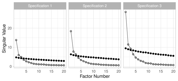
Figure 2: Largest Singular Values in Descending Order

The twenty largest singular values for $\mathfrak{P}_{\mathcal{D}}^{\phantom{\perp}}(\mathbf{\ddot{W}}(\hat{\beta},\hat{\boldsymbol{\gamma}}))\,/\sqrt{NT}$ are denoted by non-filled dots and those for permuted data by filled dots. The values for permuted data are based on 199 replications. The initial estimator for $\beta$ and $\boldsymbol{\gamma}$ uses $R=10$.

Table 8 summarizes the results of different additive and interactive fixed effects estimators (Interactive). As [1], we report results for the fixed effects estimator (Within), the Arellano-Bond estimator (AB, see [5]), and the Hahn-Hausman-Kuersteiner estimator (HHK, see [31]). However, instead of the conventional fixed effects estimator used by the authors, we report results of a bias-corrected within estimator with bandwidth $L=5$ that accounts for the asymptotic bias induced by the predetermined regressor (see [44]). For Interactive, we report results for $R\in\{1,2,3\}$. To correct for the [44] bias and those biases induced by cross-sectional heteroskedasticity and time-serial correlation, we use the asymptotic bias corrections proposed by b2009mw2017 with $L=5$ and $M=3$. Similar to [1], we report estimates and standard errors of the short- and long-run effects of democratization and the persistence of GDP processes. Further, all standard errors are heteroskedasticity robust and clustered at the country level to allow for arbitrary patterns of time-serial correlation. We find that all estimators reveal a strong and significant persistence of GDP processes across all specifications. The coefficients of democratization obtained by Within and Interactive with $R\geq 2$ are always significant at the 5 % level, whereas those of AB and HHK are only significant for $p=4$. If we focus on $p=4$, which is [1]’s preferred specification, the fixed effects models used by the authors reveal short-run effects of a transition to democracy between 0.828 % and 1.178 % and long-run effects between 16.448 % and 29.262 %. However, after controlling for additional time-varying unobserved heterogeneity, we find short- and long-run effects that are substantially lower compared to those reported by the authors. Our preferred Interactive with $R=3$, yields short- and long-run estimates of 0.622 % and 18.264 %.

Table 8: Effect of Democracy on Logarithmic GDP per Capita $(\times 100)$

	Within	AB	HHK	Interactive
				$R=1$	$R=2$	$R=3$
	Specification 1 - $p=1$
Democracy	1.051	0.959	0.781	0.745	0.755	0.809
	(0.293)	(0.477)	(0.455)	(0.329)	(0.287)	(0.305)
Persistence of	0.983	0.946	0.938	0.960	0.973	0.967
GDP process	(0.006)	(0.009)	(0.011)	(0.007)	(0.006)	(0.007)
Long-run effect	60.489	17.608	12.644	18.644	27.690	24.546
of democracy	(28.073)	(10.609)	(8.282)	(9.460)	(12.250)	(11.131)
	Specification 2 - $p=2$
Democracy	0.671	0.797	0.582	0.488	0.554	0.559
	(0.247)	(0.417)	(0.387)	(0.292)	(0.263)	(0.279)
Persistence of	0.975	0.946	0.941	0.956	0.968	0.966
GDP process	(0.005)	(0.009)	(0.010)	(0.007)	(0.005)	(0.006)
Long-run effect	26.513	14.882	9.929	11.030	17.258	16.557
of democracy	(12.026)	(9.152)	(7.258)	(7.174)	(8.881)	(9.005)
	Specification 3 - $p=4$
Democracy	0.828	0.875	1.178	0.513	0.600	0.622
	(0.225)	(0.374)	(0.370)	(0.267)	(0.259)	(0.249)
Persistence of	0.972	0.947	0.953	0.958	0.964	0.966
GDP process	(0.005)	(0.009)	(0.009)	(0.006)	(0.006)	(0.005)
Long-run effect	29.262	16.448	25.032	12.226	16.749	18.264
of democracy	(10.281)	(8.436)	(10.581)	(6.780)	(7.956)	(8.030)

• Note: Within, Ab, HHK, and Interactive denote the bias-corrected fixed effects estimator, the Arellano-Bond estimator, the Hahn-Hausman-Kuersteiner estimator, and the IFE estimator. Standard errors in parentheses are heteroskedasticity robust and clustered at the country level. Within and Interactive use bandwidths $L=5$ and $M=3$ for the estimation of the asymptotic biases. The results of AB and HHK are taken from table 2 in [1].

Next we consider two different sensitivity checks. First, the estimation of the asymptotic biases requires different bandwidth choices. We check the sensitivity of the results by analyzing all combinations of the following bandwidth choices: $L\in\{1,\ldots,7\}$ and $M\in\{1,\ldots,7\}$. Second, we report estimates of Interactive for $R\in\{4,\ldots,10\}$. As shown by [37], the inclusion of additional redundant common factors should only affect the precision of the IFE estimator after controlling for all relevant common factors. Table 9 and 10 summarize the results. With respect to the different bandwidth choices, we find that the results of Interactive are very robust to all combinations of bandwidth choices as indicated by the narrow intervals reported in the table. Contrary, the estimates of Within are more sensitive. For $p=4$, we find long-run effects between 21.571 % and 32.289 %. With respect to the number of factors, we find that after controlling for more than three, the estimated persistence of the GDP process starts declining. The same pattern was also recognized in the empirical illustration of [37]. The authors argue that the dynamic specification might be misspecified in the sense that the lagged outcome variables simply capture time-serial correlation in the idiosyncratic error term instead of true state dependence. Because the factor structure also captures time-serial correlation, this might indicate that there is no true state dependence. Contrary the coefficients of democratization become larger and remain significant in most specifications.

Table 9: Sensitivity to Different Bandwidth Choices

	Within	Interactive
		$R=1$	$R=2$	$R=3$
	Specification 1 - $p=1$
Democracy	[0.986; 1.057]	[0.744; 0.775]	[0.755; 0.806]	[0.806; 0.867]
Persistence of	[0.974; 0.984]	[0.958; 0.960]	[0.972; 0.973]	[0.966; 0.968]
GDP process
Long-run effect	[38.127; 64.280]	[18.551; 18.872]	[27.336; 29.065]	[24.368; 25.713]
of democracy
	Specification 2 - $p=2$
Democracy	[0.633; 0.674]	[0.488; 0.522]	[0.554; 0.609]	[0.548; 0.583]
Persistence of	[0.968; 0.976]	[0.954; 0.956]	[0.967; 0.968]	[0.966; 0.967]
GDP process
Long-run effect	[19.509; 27.723]	[10.987; 11.369]	[17.231; 18.721]	[16.158; 17.150]
of democracy
	Specification 3 - $p=4$
Democracy	[0.773; 0.849]	[0.504; 0.547]	[0.596; 0.635]	[0.620; 0.661]
Persistence of	[0.964; 0.974]	[0.957; 0.958]	[0.964; 0.964]	[0.965; 0.966]
GDP process
Long-run effect	[21.571; 32.289]	[11.945; 12.672]	[16.548; 17.715]	[18.113; 19.352]
of democracy

• Note: Effect of democracy on logarithmic GDP per capita $(\times 100)$. Within and Interactive denote the bias-corrected fixed effects estimator and the IFE estimator. The intervals denote the ranges of all estimates across different combinations of $L\in\{1,\ldots,7\}$ and $M\in\{1,\ldots,7\}$.

Table 10: Sensitivity to the Number of Factors

	$R=4$	$R=5$	$R=6$	$R=7$	$R=8$	$R=9$	$R=10$
	Specification 1 - $p=1$
Democracy	0.417	0.160	1.101	1.553	1.615	1.619	2.197
	(0.511)	(0.486)	(0.516)	(0.564)	(0.602)	(0.634)	(0.718)
Persistence of	0.848	0.854	0.754	0.702	0.600	0.554	0.453
GDP process	(0.018)	(0.020)	(0.030)	(0.035)	(0.034)	(0.039)	(0.040)
Long-run effect	2.749	1.095	4.476	5.220	4.037	3.635	4.019
of democracy	(3.363)	(3.339)	(2.140)	(1.939)	(1.551)	(1.479)	(1.394)
	Specification 2 - $p=2$
Democracy	0.388	0.868	1.178	1.424	1.905	1.150	1.418
	(0.469)	(0.446)	(0.511)	(0.565)	(0.614)	(0.651)	(0.705)
Persistence of	0.810	0.689	0.586	0.485	0.369	0.342	0.247
GDP process	(0.019)	(0.031)	(0.036)	(0.031)	(0.038)	(0.042)	(0.056)
Long-run effect	2.041	2.795	2.845	2.767	3.019	1.747	1.882
of democracy	(2.478)	(1.458)	(1.266)	(1.129)	(1.013)	(1.018)	(0.968)
	Specification 3 - $p=4$
Democracy	0.763	1.091	1.452	1.474	1.513	1.474	0.476
	(0.455)	(0.446)	(0.534)	(0.567)	(0.557)	(0.596)	(0.589)
Persistence of	0.628	0.593	0.380	0.213	0.174	0.187	-0.202
GDP process	(0.025)	(0.038)	(0.049)	(0.050)	(0.056)	(0.092)	(0.075)
Long-run effect	2.053	2.683	2.341	1.874	1.831	1.814	0.396
of democracy	(1.211)	(1.124)	(0.883)	(0.729)	(0.692)	(0.766)	(0.493)

• Note: Effect of democracy on logarithmic GDP per capita $(\times 100)$. Results obtained by the interactive fixed effects estimator for $R\in\{4,\ldots,10\}$. Standard errors in parentheses are heteroskedasticity robust and clustered at the country level. Bandwidths $L=5$ and $M=3$ for the estimation of the asymptotic biases.

Finally, we consider an additional specification without predetermined regressors ($p=0$). Again we estimate the number of factors from a pure factor model, where the initial estimate is based on $R=10$. The estimates are identical to those of $p=4$ and provide further support for our preferred choice of $R=3$. The corresponding estimate of democratization is - 1.251 % (standard error = 1.286 %) and is in line with [12] who report a negative and/or insignificant effect of democracy on growth.

To sum up, we find some additional support for the hypothesis of [1]: democracy does cause growth. Using the IFE estimator to control for time-varying unobserved heterogeneity, we obtain results that are qualitatively similar to the authors. If we compare HHK to Interactive with $R=3$ in the authors preferred specification $p=4$, we find that the short-run effect of democratization is halved. However the corresponding long-run effect of 18.264 % is still pretty close to the 20 % reported by [1].

Further Extensions

Although we analyzed the IFE estimator of [7], we want to point out two natural extensions of our findings. First, in the presence of regressors that are endogenous with respect to the idiosyncratic error term, mw2017msw2018 suggest a minimum distance estimator with interactive fixed effects in the spirit of ch2006ch2008. Second, because the objective function of the IFE estimator is generally non-convex, [39] suggest an alternative estimator that avoids the potentially difficult optimization problem with multiple local minima and results in optimizing a convex objective function.

Extension 1: Minimum Distance Estimator

Suppose that $\mathbf{x}_{it}$ can be further decomposed into $K_{1}$ endogenous and $K_{2}$ exogenous regressors such that $K=K_{1}+K_{2}$. To avoid ambiguity, we label endogenous and exogenous regressors with an appropriate superscript. Further, let $\mathbf{z}_{it}=[z_{it,1},\ldots,z_{it,M}]$ be a vector of excluded exogenous instruments with $M\geq K_{1}$. [38] suggest the following minimum distance estimator. In a first step, an estimator for $\boldsymbol{\beta}^{\text{end}}$ is obtained by

$$\hat{\boldsymbol{\beta}}^{\text{end}}=\underset{\boldsymbol{\beta}^{\text{end}}\in\mathbb{R}^{K_{1}}}{\operatorname{\arg\,\min\;}}\hat{\boldsymbol{\pi}}\left(\boldsymbol{\beta}^{\text{end}}\right)^{\prime}\,\boldsymbol{\Sigma}\,\hat{\boldsymbol{\pi}}\left(\boldsymbol{\beta}^{\text{end}}\right)\,,$$ (22)

where $\hat{\boldsymbol{\pi}}(\boldsymbol{\beta}^{\text{end}})$ is the IFE estimator of

$$y_{it}-\mathbf{x}_{it}^{\text{end}\,\prime}\boldsymbol{\beta}^{\text{end}}=\mathbf{x}_{it}^{\text{exo}\,\prime}\boldsymbol{\beta}^{\text{exo}}+\mathbf{z}_{it}^{\prime}\boldsymbol{\pi}+\boldsymbol{\lambda}_{i}^{\prime}\mathbf{f}_{t}^{\phantom{\prime}}+e_{it}$$ (23)

and $\boldsymbol{\Sigma}$ is a positive definite $M\times M$ weighting matrix. At the true value of $\boldsymbol{\beta}^{\text{end}}$, $\boldsymbol{\pi}$ is zero given the exclusion restriction on $\mathbf{z}_{it}$. In a second step, $\hat{\boldsymbol{\beta}}^{\text{exo}}$ is the IFE estimator of

$$y_{it}-\mathbf{x}_{it}^{\text{end}\,\prime}\hat{\boldsymbol{\beta}}^{\text{end}}=\mathbf{x}_{it}^{\text{exo}\,\prime}\boldsymbol{\beta}^{\text{exo}}+\boldsymbol{\lambda}_{i}^{\prime}\mathbf{f}_{t}^{\phantom{\prime}}+e_{it}\,.$$ (24)

The properties of the minimum distance estimator are studied in [36], where the authors extend the random coefficient demand model of [13] with interactive fixed effects to account for unobserved product-market specific heterogeneity, like advertisement. Under very similar assumptions as in [38], the authors show consistency and derive the asymptotic distribution of the minimum distance estimator. Because their estimator embeds the IFE estimator, we can apply the same algorithms and estimators studied in this article. Further, [35] use the same estimator to account for measurement errors in the dependent variable in dynamic interactive fixed effects models.

Extension 2: Nuclear Norm Minimizing Estimator

[39] show that the imposed rank constraint on the factor structure leads to a non-convex optimization problem. The authors suggest an alternative estimator based on a convex relaxation of this constraint. More precisely, they show that an estimator for $\boldsymbol{\beta}$ is

$$\hat{\boldsymbol{\beta}}^{\star}=\underset{\boldsymbol{\beta}\in\mathbb{R}^{K}}{\operatorname{\arg\,\min\;}}\frac{1}{2n}\sum_{r=1}^{\min(N,T)}\sigma_{r}\left[\mathfrak{P}_{\mathcal{D}}^{\phantom{\perp}}\left(\mathbf{W}\left(\boldsymbol{\beta}\right)\right)\right]\,,$$ (25)

where $\sigma_{r}[\cdot]$ denotes the $r$-th largest singular value. [39] show consistency of this estimator, but only at a rate of $\sqrt{\min(N,T)}$. As a consequence, the convex relaxation leads to a certain loss of efficiency compared to the IFE estimator.

To recover the properties of the IFE estimator, [39] suggest to estimate the number of factors from $\mathfrak{P}_{\mathcal{D}}^{\phantom{\perp}}(\mathbf{W}(\hat{\boldsymbol{\beta}}^{\star}))$ and afterwards apply an iterative post estimation routine. After a finite number of iterations the estimator has the same limiting distribution as the IFE estimator. The post estimation routine can be summarized as follows:

Definition.

Post nuclear norm estimation

Given $\hat{\boldsymbol{\beta}}^{\star}$ and $R$, initialize $\hat{\boldsymbol{\beta}}=\hat{\boldsymbol{\beta}}^{\star}$ and repeat the following steps a finite number of times

• Compute $\widehat{\mathbf{F}}\left(\hat{\boldsymbol{\beta}}\right)$ and $\widehat{\boldsymbol{\Lambda}}\left(\hat{\boldsymbol{\beta}}\right)$ from $\widetilde{\mathbf{W}}\left(\hat{\boldsymbol{\beta}}\right)$

• Compute $\breve{\mathbf{y}}$ and $\breve{\mathbf{x}}_{k}$ for all $k\in\{1,\ldots,K\}$

• Update $\hat{\boldsymbol{\beta}}=\left(\breve{\mathbf{X}}^{\prime}\breve{\mathbf{X}}\right)^{-1}\breve{\mathbf{X}}^{\prime}\breve{\mathbf{y}}$, where $\breve{\mathbf{X}}=[\breve{\mathbf{x}}_{1},\ldots,\breve{\mathbf{x}}_{K}]$

Conclusion

The assumption that unobserved heterogeneity is constant over time, is often very restrictive. Especially in panels that cover a long time horizon, like macroeconomic panels of countries, it is unlikely that a global shock affects all countries equally. Interactive fixed effects estimators offer researchers new possibilities to consider this more general form of heterogeneity in their analysis (see among others hnr1988p2006b2009). However these panels are often naturally unbalanced, demanding an additional data augmentation step for the estimator of [7] (see Appendix of [7] and [9]).

In this article, we analyzed the finite sample behavior of [7]’s interactive fixed effects estimator in the presence of randomly missing data. Simulation experiments confirmed that the inferential theory derived by b2009mw2017 for balanced data also provides a reasonable approximation for the unbalanced case. However, we also found that the finite sample performance can be affected by the fraction and pattern of missing data.

Future research could address this issue and provide an inferential theory, which takes the additional uncertainty induced by data augmentation into account. This might help to improve the finite sample behavior of [7]’s estimator in the presence of randomly missing data.

References

- [1] Daron Acemoglu, Suresh Naidu, Pascual Restrepo and James A. Robinson “Democracy Does Cause Growth” In Journal of Political Economy 127.1, 2019, pp. 47–100
- [2] Seung C. Ahn and Alex R. Horenstein “Eigenvalue Ratio Test for the Number of Factors” In Econometrica 81.3, 2013, pp. 1203–1227
- [3] Lucia Alessi, Matteo Barigozzi and Marco Capasso “Improved penalization for determining the number of factors in approximate factor models” In Statistics & Probability Letters 80.23, 2010, pp. 1806–1813
- [4] T.W. Anderson and Cheng Hsiao “Formulation and estimation of dynamic models using panel data” In Journal of Econometrics 18.1, 1982, pp. 47–82
- [5] Manuel Arellano and Stephen Bond “Some Tests of Specification for Panel Data: Monte Carlo Evidence and an Application to Employment Equations” In The Review of Economic Studies 58.2, 1991, pp. 277–297
- [6] Jushan Bai “Inferential Theory for Factor Models of Large Dimensions” In Econometrica 71.1, 2003, pp. 135–171
- [7] Jushan Bai “Panel Data Models with Interactive Fixed Effects” In Econometrica 77.4, 2009, pp. 1229–1279
- [8] Jushan Bai and Yuan Liao “Inferences in panel data with interactive effects using large covariance matrices” In Journal of Econometrics 200.1, 2017, pp. 59–78
- [9] Jushan Bai, Yuan Liao and Jisheng Yang “Unbalanced Panel Data Models with Interactive Effects” In The Oxford Handbook of Panel Data, 2015, pp. 149–170
- [10] Jushan Bai and Serena Ng “Determining the Number of Factors in Approximate Factor Models” In Econometrica 70.1, 2002, pp. 191–221
- [11] Jushan Bai and Serena Ng “Principal components estimation and identification of static factors” In Journal of Econometrics 176.1, 2013, pp. 18–29
- [12] Robert J. Barro “Democracy and Growth” In Journal of Economic Growth 1.1, 1996, pp. 1–27
- [13] Steven Berry, James Levinsohn and Ariel Pakes “Automobile Prices in Market Equilibrium” In Econometrica 63.4, 1995, pp. 841–890
- [14] Stéphane Bonhomme and Elena Manresa “Grouped Patterns of Heterogeneity in Panel Data” In Econometrica 83.3, 2015, pp. 1147–1184
- [15] Andreas Buja and Nermin Eyuboglu “Remarks on Parallel Analysis” In Multivariate Behavioral Research 27.4, 1992, pp. 509–540
- [16] Gary Chamberlain “Multivariate regression models for panel data” In Journal of Econometrics 18.1, 1982, pp. 5–46
- [17] Gary Chamberlain “Chapter 22 Panel data” 2, Handbook of Econometrics, 1984, pp. 1247–1318
- [18] Mingli Chen, Iván Fernández-Val and Martin Weidner “Nonlinear Factor Models for Network and Panel Data” In arXiv preprint arXiv: 1412.5647, 2019
- [19] Shuowen Chen, Victor Chernozhukov and Iván Fernández-Val “Mastering Panel Metrics: Causal Impact of Democracy on Growth” In AEA Papers and Proceedings 109, 2019, pp. 77–82
- [20] Victor Chernozhukov and Christian Hansen “Instrumental quantile regression inference for structural and treatment effect models” In Journal of Econometrics 132.2, 2006, pp. 491–525
- [21] Victor Chernozhukov and Christian Hansen “Instrumental variable quantile regression: A robust inference approach” In Journal of Econometrics 142.1, 2008, pp. 379–398
- [22] In Choi and Hanbat Jeong “Model selection for factor analysis: Some new criteria and performance comparisons” In Econometric Reviews 38.6, 2019, pp. 577–596
- [23] Daniel Czarnowske and Amrei Stammann “Binary Choice Models with High-Dimensional Individual and Time Fixed Effects” In arXiv preprint arXiv:1904.04217, 2019
- [24] Edgar Dobriban “Permutation methods for factor analysis and PCA” In Annals of Statistics, forthcoming
- [25] Edgar Dobriban and Art B. Owen “Deterministic parallel analysis: an improved method for selecting factors and principal components” In Journal of the Royal Statistical Society: Series B (Statistical Methodology) 81.1, 2019, pp. 163–183
- [26] Iván Fernández-Val and Martin Weidner “Fixed Effects Estimation of Large-T Panel Data Models” In Annual Review of Economics 10.1, 2018, pp. 109–138
- [27] David Chin-Lung Fong and Michael Saunders “LSMR: An Iterative Algorithm for Sparse Least-Squares Problems” In SIAM Journal on Scientific Computing 33.5, 2011, pp. 2950–2971
- [28] Patrick Gagliardini, Elisa Ossola and Olivier Scaillet “A diagnostic criterion for approximate factor structure” In Journal of Econometrics 212.2, 2019, pp. 503–521
- [29] Simen Gaure “OLS with multiple high dimensional category variables” In Computational Statistics & Data Analysis 66, 2013, pp. 8–18
- [30] Paulo Guimarães and Pedro Portugal “A simple feasible procedure to fit models with high-dimensional fixed effects” In Stata Journal 10.4, 2010, pp. 628–649
- [31] Jinyong Hahn, Jerry Hausman and Guido Kuersteiner “Estimation with weak instruments: Accuracy of higher-order bias and MSE approximations” In The Econometrics Journal 7.1, 2004, pp. 272–306
- [32] Marc Hallin and Roman Liška “Determining the Number of Factors in the General Dynamic Factor Model” In Journal of the American Statistical Association 102.478, 2007, pp. 603–617
- [33] Israel Halperin “The product of projection operators” In Acta Sci. Math. (Szeged) 23, 1962, pp. 96–99
- [34] Douglas Holtz-Eakin, Whitney Newey and Harvey S. Rosen “Estimating Vector Autoregressions with Panel Data” In Econometrica 56.6, 1988, pp. 1371–1395
- [35] Nayoung Lee, Hyungsik Roger Moon and Martin Weidner “Analysis of interactive fixed effects dynamic linear panel regression with measurement error” In Economics Letters 117.1, 2012, pp. 239–242
- [36] Hyungsik Roger Moon, Matthew Shum and Martin Weidner “Estimation of random coefficients logit demand models with interactive fixed effects” In Journal of Econometrics 206.2, 2018, pp. 613–644
- [37] Hyungsik Roger Moon and Martin Weidner “Linear Regression for Panel With Unknown Number of Factors as Interactive Fixed Effects” In Econometrica 83.4, 2015, pp. 1543–1579
- [38] Hyungsik Roger Moon and Martin Weidner “DYNAMIC LINEAR PANEL REGRESSION MODELS WITH INTERACTIVE FIXED EFFECTS” In Econometric Theory 33.1, 2017, pp. 158–195
- [39] Hyungsik Roger Moon and Martin Weidner “Nuclear Norm Regularized Estimation of Panel Regression Models” In arXiv preprint arXiv: 1810.10987, 2019
- [40] Yair Mundlak “On the Pooling of Time Series and Cross Section Data” In Econometrica 46.1, 1978, pp. 69–85
- [41] Whitney K. Newey and Richard J. Smith “Higher Order Properties of GMM and Generalized Empirical Likelihood Estimators” In Econometrica 72.1, 2004, pp. 219–255
- [42] Whitney K. Newey and Kenneth D. West “A Simple, Positive Semi-Definite, Heteroskedasticity and Autocorrelation Consistent Covariance Matrix” In Econometrica 55.3, 1987, pp. 703–708
- [43] Whitney K. Newey and Kenneth D. West “Automatic Lag Selection in Covariance Matrix Estimation” In The Review of Economic Studies 61.4, 1994, pp. 631–653
- [44] Stephen Nickell “Biases in Dynamic Models with Fixed Effects” In Econometrica 49.6, 1981, pp. 1417–1426
- [45] Alexei Onatski “Determining the Number of Factors from Empirical Distribution of Eigenvalues” In The Review of Economics and Statistics 92.4, 2010, pp. 1004–1016
- [46] M. Pesaran “Estimation and Inference in Large Heterogeneous Panels with a Multifactor Error Structure” In Econometrica 74.4, 2006, pp. 967–1012
- [47] R Core Team “R: A Language and Environment for Statistical Computing”, 2019 R Foundation for Statistical Computing URL: https://www.R-project.org/
- [48] G. Schwert “Tests for Unit Roots: A Monte Carlo Investigation” In Journal of Business & Economic Statistics 7.2, 1989, pp. 147–159
- [49] Amrei Stammann “Fast and feasible estimation of generalized linear models with high-dimensional k-way fixed effects” In arXiv preprint arXiv:1707.01815, 2018
- [50] James H. Stock and Mark W. Watson “Diffusion indexes” In NBER Working Paper No. 6702, 1998
- [51] James H. Stock and Mark W. Watson “Macroeconomic forecasting using diffusion indexes” In Journal of Business & Economic Statistics 20.2, 2002, pp. 147–162
- [52] Halbert White “A Heteroskedasticity-Consistent Covariance Matrix Estimator and a Direct Test for Heteroskedasticity” In Econometrica 48.4, 1980, pp. 817–838