Testing the equality of spectral density operators for functional processes

Abstract

The problem of comparing the entire second order structure of two functional processes is considered and a $L^{2}$-type statistic for testing equality of the corresponding spectral density operators is investigated. The test statistic evaluates, over all frequencies, the Hilbert-Schmidt distance between the two estimated spectral density operators. Under certain assumptions, the limiting distribution under the null hypothesis is derived. A novel frequency domain bootstrap method is introduced, which leads to a more accurate approximation of the distribution of the test statistic under the null than the large sample Gaussian approximation derived. Under quite general conditions, asymptotic validity of the bootstrap procedure is established for estimating the distribution of the test statistic under the null. Furthermore, consistency of the bootstrap-based test under the alternative is proved. Numerical simulations show that, even for small samples, the bootstrap-based test has a very good size and power behavior. An application to a bivariate real-life functional time series illustrates the methodology proposed.

1 Introduction

Functional data analysis is a branch of statistics that in recent years has grown considerably and has created great research interest in the scientific community, especially in connection with the increasing number of situations in which theoretical and applied scientists have to deal with data of a continuous nature (i.e., curves, images, surfaces, etc.). For various works and references in different branches of functional data analysis, we refer to the recent special issues of Goia and Vieu [14] and Aneiros et al. [1]. See also the monograph by Horváth & Kokoszka [17] which discusses inference problems in a variety of setting concerning independent as well as dependent functional data.

In our work, we focus on dependent functional data and, in particular, on functional time series analysis. Functional time series occurs in many applications such as daily curves of financial transactions, daily images of geophysical and environmental data and daily curves of temperature measurements. Such curves or images are viewed as functions in appropriate spaces since an observed intensity is available at each point on a line segment, a portion of a plane or a volume. Moreover, and most importantly, such functional time series exhibit temporal dependence and ignoring this dependence may result in misleading conclusions and not approperiate inferential procedures.

Comparing characteristics of two or more groups of functional data forms an important problem of statistical inference with a variety of applications. For instance, comparing the mean functions between independent groups of independent and identically distributed (i.i.d.) functional data has attracted considerable interest in the literature, see, e.g., Benko et al. [3], Zhang et al. [38], Horváth and Kokoszka [17] (Chapter 5), Horváth et al. [18] and Paparoditis and Sapatinas [24]. In contrast to comparing mean functions, the problem of comparing the entire second order structure of two independent functional time series has been much less investigated. Notice that for i.i.d. functional data this problem simplifies to the problem of testing the equality of (the lag zero) covariance operators, see, e.g., Panaretos et al. [21], Fremdt et al. [13], Pigoli et al. [26] and Paparoditis and Sapatinas [24]. The same problem of testing the equality of the (lag-zero) covariance operators of two sets of independent functional time series has also been investigated by Zhang and Shao [37] and by Pilvakis et al. [28].

However, the comparison of the entire second order structure of independent functional time series, is a much more involved problem due to the temporal dependence between the random elements considered. In describing the second order structure of functional time series, the spectral density operator, introduced in the functional set-up by Panaretos and Tavakoli [22], is a very useful tool since it summarizes in a nice way the entire autocovariance structure of the underlying functional time series; see also Hörmann et al. [16]. It is, therefore, very appealing to develop a spectral approach for testing equality of the entire second order structure of two functional time series. Tavakoli and Panaretos [34] proposed an approach based on projections on finite dimensional spaces of the differences of the estimated spectral density operators of the two functional time series. Projection-based tests have the advantage to lead to manageable limiting distributions. However, such tests have no power for alternatives which are orthogonal to the projection space considered. Furthermore, the number of projections appears as an additional tuning parameter which has to be chosen by the user. Finally, simulations in the much simpler i.i.d. set-up suggest that the quality of the large sample Gaussian approximations of the corresponding test, is affected by the number of projections used; see Paparoditis and Sapatinas [24]. In this paper we focus on tests which evaluate the differences between the entire, infinite dimensional, structure of the two spectral density operators compared. For this, the Hilbert-Schmidt norm of the differences between the estimated spectral density operators, evaluated over all frequencies, is used as the basic building block of the test statistic considered.

The contribution of this paper is twofold. First, we focus on testing the equality of the entire second order structure between two independent functional processes by evaluating for each frequency, the Hilbert-Schmidt norm between the (estimated) spectral density operators of the functional process at hand. Integrating these differences over all possible frequencies, leads to a global, $L^{2}$-type, measure of deviation which is used to test the null hypothesis of interest. We show that under the assumption of a linear Hilbertian processes, the limiting distribution of an appropriately centered version of such a test statistic under the null, is Gaussian. This Gaussian distribution does not depend on characteristics of the underlying functional processes beyond those of second order. Second, and because of the slow convergence of the distribution of the considered $L^{2}$-type test statistic under the null against the derived limiting Gaussian distribution, we develop a novel frequency domain bootstrap procedure to estimate this distribution. The frequency domain bootstrap method works under minimal conditions on the underlying functional process and its range of applicability is not restricted to the particular class of processes considered and which is used to derive the limiting distribution of our test. We prove under very general conditions, that the bootstrap procedure correctly approximates the distribution of the proposed test statistic under the null. Furthermore, consistency of the bootstrap-based test under the alternative is established. Our theoretical deviations are accompanied by a simulation study which shows a very good behavior of the bootstrap procedure in approximating the distribution of interest and the good size and power performance of the test based on bootstrap critical values. Notice that the frequency domain bootstrap method proposed in this paper, can potentially be used to improve the performance of other tests too, like for instance, the projections based test of Tavakoli and Panaretos [34].

Developing bootstrap procedures for functional time series has attracted considerable interest in the literature. Politis and Romano [29] established weak convergence results for the stationary bootstrap, Dehling et al. [7] for the (non-overlapping) block bootstrap in a testing context, Raña et al. [30] applied a stationary bootstrap to functional time series, Ferraty and Vieu [10] a residual-based bootstrap and Franke and Nyarige [12] established consistency of a model-based bootstrap for functional autoregressions. Pilavakis et al. [27] derived theoretical results for the moving block bootstrap and for the tapered block bootstrap, Shang [32] applied a maximum entropy bootstrap and Paparoditis [25] introduced a sieve bootstrap for functional time series. In contrast to the aforementioned contributions, the bootstrap procedure proposed in this paper acts solely in the frequency domain and generates replicates of the periodogram kernels stemming from functional processes that satisfy the null hypothesis of interest.

A test related to ours and proposed after the first preprint of this paper has been appeared (see Leucht et al. [20]), is that of van Delft and Dette [35], which deals with testing a different set of hypotheses, so-called relevant hypotheses, about the second order dynamics of two functional processes. Important differences between the two procedures appear which will be discussed in more detail later on. However, we stress here the fact that the test statistic proposed in this paper is not a special case of the test statistic used in the aforementioned paper and, consequently, the limiting distribution of our test statistic is different and not covered by the asymptotic results derived in that paper. See Remark et al. for more details.

The remainder of the paper is organized as follows. Section 2 contains the main assumptions on the underlying functional linear processes and states the hypothesis testing problem under study. Section 3 is devoted to the suggested test statistic and its asymptotic behavior while Section 4 presents the frequency domain bootstrap procedure proposed to estimate the distribution of the test statistic under the null. Asymptotic validity of the bootstrap procedure is established and consistency of the corresponding test under the alternative also is proved. Section 5 contains numerical simulations and an application to a bivariate meteorological functional time series while Section 6 concludes our findings. Auxiliary results containing some new results on frequency domain properties of linear Hilbertian processes as well as proofs of the main results are deferred to the Appendix and to the Supplementary Material.

2 Assumptions and the Testing Problem

Suppose that observations $X_{1},\dots,X_{T}$ and $Y_{1},\dots,Y_{T}$ stem from functional processes $(X_{t})_{t\in{\mathbb{Z}}}$ and $(Y_{t})_{t\in{\mathbb{Z}}}$, respectively, satisfying the following assumption.

Assumption 1 : $(X_{t})_{t\in{\mathbb{Z}}}$ and $(Y_{t})_{t\in{\mathbb{Z}}}$ are independent functional linear processes, given by

$$X_{t}=\sum_{j\in{\mathbb{Z}}}A_{j}(\varepsilon_{t-j})\quad\text{and}\quad Y_{t}=\sum_{j\in{\mathbb{Z}}}B_{j}(e_{t-j}),\;t\in{\mathbb{Z}},$$ (1)

with values in $L^{2}_{\mathbb{R}}([0,1],\mu)$, where $\mu$ denotes the Lebesgue measure. The innovation functions $(\varepsilon_{t})_{t\in{\mathbb{Z}}}$ and $(e_{t})_{t\in{\mathbb{Z}}}$ are two i.i.d. mean zero Gaussian processes with values in $L^{2}_{\mathbb{R}}([0,1],\mu)$ and covariance operators $C_{\varepsilon}$ and $C_{e}$ with continuous covariance kernels $c_{\varepsilon}$ and $c_{e}$, respectively. The sequences $(A_{j})_{j\in{\mathbb{Z}}}$ and $(B_{j})_{j\in{\mathbb{Z}}}$ of bounded linear operators from $L^{2}_{\mathbb{R}}([0,1],\mu)$ to $L^{2}_{\mathbb{R}}([0,1],\mu)$ where $A_{0}=B_{0}$ is the identity operator, satisfy $\sum_{j\in{\mathbb{Z}}}|j|(\|A_{j}\|_{\mathcal{L}}+\|B_{j}\|_{\mathcal{L}})<\infty$ with $\|\cdot\|_{\mathcal{L}}$ denoting the operator norm.

We are interested in testing for equality of the entire second order structure of the two functional processes given in (1). Notice that considering linear processes in Assumption 1 should not be considered as restrictive since our interest is solely focused on the comparison of the second order structure, i.e., of the autocovariance structure of the underlying functional processes. Furthermore, and as we will see later on, the assumption of Gaussian innovation functions $\varepsilon_{t}$ and $e_{t}$ is not essential. It is solely imposed in order to simplify the already quite involved technical arguments used to derive the limiting distribution of the test.

For the testing problem considered it turns out that a spectral approach is very appealing. Towards this notice first that we can define a spectral density operator in the sense of Panaretos and Tavakoli [22] in the present set up which generalizes the concept of spectral densities for univariate time series and spectral density matrices for multivariate time series. Here and in the sequel, we will abbreviate $L^{2}_{\mathbb{R}}([0,1]^{d},\mu)$ by $L^{2}$ if the dimension $d$ becomes clear from the context.

Lemma 1.

Suppose that $(X_{t})_{t\in{\mathbb{Z}}}$ and $(Y_{t})_{t\in{\mathbb{Z}}}$ are functional processes satisfying Assumption 1. Then, for arbitrary $\lambda\in(-\pi,\pi]$,

$$f_{X,\lambda}(\cdot,\cdot)=\frac{1}{2\pi}\sum_{t\in{\mathbb{Z}}}e^{-i\lambda t}\,r_{X,t}(\cdot,\cdot),\quad f_{Y,\lambda}(\cdot,\cdot)=\frac{1}{2\pi}\sum_{t\in{\mathbb{Z}}}{e^{-i\lambda t}}\,r_{Y,t}(\cdot,\cdot)$$

with $r_{X,t}$ and $r_{Y,t}$ denoting the autocovariance kernels of $X$ and $Y$ at lag $t$, respectively, converge absolutely in $L^{2}$. Moreover, for all $\sigma,\tau\in[0,1]$,

$$r_{X,t}(\sigma,\tau)=\int_{(-\pi,\pi]}f_{X,\lambda}(\sigma,\tau)\,{e^{i\lambda t}}\,d\lambda,\quad r_{Y,t}(\sigma,\tau)=\int_{(-\pi,\pi]}f_{Y,\lambda}(\sigma,\tau)\,{e^{i\lambda t}}\,d\lambda\quad\forall t\in\mathbb{Z},$$

where equality holds in $L^{2}$. The operators ${\mathcal{F}_{X,\lambda}}$ and ${\mathcal{F}_{Y,\lambda}}$, induced by right integration of $f_{X,\lambda}$ and $f_{Y,\lambda}$, are self-adjoint, nonnegative definite and it holds

$$\mathcal{F}_{X,\lambda}=\frac{1}{2\pi}\sum_{t\in{\mathbb{Z}}}e^{-i\lambda t}\mathcal{R}_{X,t},\quad\mathcal{F}_{Y,\lambda}=\frac{1}{2\pi}\sum_{t\in{\mathbb{Z}}}e^{-i\lambda t}\mathcal{R}_{Y,t},$$

where $\mathcal{R}_{X,t}$ and $\mathcal{R}_{Y,t}$ denote the autocovariance operators of $X$ and $Y$ at lag $t$, induced by right integration of $r_{X,t}$ and $r_{Y,t}$, respectively. Convergence holds in nuclear norm.

The kernels $f_{X,\lambda}$ and $f_{Y,\lambda}$ are called the spectral density kernels (at frequency $\lambda$) and the operators $\mathcal{F}_{X,\lambda}$ and $\mathcal{F}_{Y,\lambda}$ are referred to as the corresponding spectral density operators.

Under the assumptions of Lemma 1, we can now state the hypothesis testing problem of interest as follows

$${\mathcal{H}_{0}}\colon\mathcal{F}_{X,\lambda}=\mathcal{F}_{Y,\lambda}\quad\text{ for }\mu\text{-}\text{almost all }\lambda\in(-\pi,\pi],$$ (2)

$${\mathcal{H}_{1}}\colon\mathcal{F}_{X,\lambda}\neq\mathcal{F}_{Y,\lambda}\quad\forall\lambda\in A\text{ for some $A\subset[0,\pi]$ with }\mu(A)>0.$$

3 The Test Statistic and its Asymptotic Behavior

We first estimate the unknown spectral density operator $\mathcal{F}_{X,\lambda}$ by an integral operator $\widehat{\mathcal{F}}_{X,\lambda}$ induced by right integration with the kernel

$$\hat{f}_{X,\lambda}(\sigma,\tau)=\frac{1}{bT}\sum_{t=-N}^{N}W\left(\frac{\lambda-\lambda_{t}}{b}\right)\,\widehat{p}_{X,\lambda_{t}}(\sigma,\tau),\;\;\mbox{for all}\;\;\sigma,\tau\in[0,1],$$

and, similarly, $\mathcal{F}_{Y,\lambda}$ by an integral operator $\widehat{\mathcal{F}}_{Y,\lambda}$ induced by right integration with the kernel

$$\hat{f}_{Y,\lambda}(\sigma,\tau)=\frac{1}{bT}\sum_{t=-N}^{N}W\left(\frac{\lambda-\lambda_{t}}{b}\right)\,\widehat{p}_{Y,\lambda_{t}}(\sigma,\tau),\;\;\mbox{for all}\;\;\sigma,\tau\in[0,1].$$

Here, $N=[(T-1)/2]$ and $\lambda_{t}=2\pi t/T,\;t\in\{-N,\dots,N\},$ denote the Fourier frequencies. Furthermore, $b=b_{T}>0$ is an asymptotically vanishing bandwidth and $W$ denotes a weight function. Moreover, as in Panaretos and Tavakoli [22],

$$\widehat{p}_{X,\lambda}(\sigma,\tau)=\frac{1}{2\pi T}\sum_{s_{1},s_{2}=1}^{T}X_{s_{1}}(\sigma)X_{s_{2}}(\tau)\,\exp(-i\lambda(s_{1}-s_{2})),\;\;\mbox{for all}\;\;\sigma,\tau\in[0,1],$$

and

$$\widehat{p}_{Y,\lambda}(\sigma,\tau)=\frac{1}{2\pi T}\sum_{s_{1},s_{2}=1}^{T}Y_{s_{1}}(\sigma)Y_{s_{2}}(\tau)\,\exp(-i\lambda(s_{1}-s_{2})),\;\;\mbox{for all}\;\;\sigma,\tau\in[0,1],$$

denote the periodogram kernels based on $X_{1},\dots,X_{T}$ and $Y_{1},\dots,Y_{T}$, respectively. The periodogram operators $I_{X,\lambda}$, and $I_{Y,\lambda}$ are defined as integral operators induced by right integration of the periodogram kernels $\widehat{p}_{X,\lambda}$ and $\widehat{p}_{Y,\lambda}$, respectively.

For the hypothesis testing problem (2), we propose the following test statistic

$${\mathcal{U}_{T}}=\int_{-\pi}^{\pi}\|\widehat{\mathcal{F}}_{X,\lambda}-\widehat{\mathcal{F}}_{Y,\lambda}\|_{HS}^{2}\,d\lambda,$$ (3)

which evaluates the distance between the estimated spectral density operators via the Hilbert-Schmidt norm $\|\cdot\|_{HS}$. The following theorem states the asymptotic properties of the suitably normalized test statistic $\mathcal{U}_{T}$ when the null hypothesis ${\mathcal{H}_{0}}$ is true.

Theorem 1.

Suppose that the stretches of observations $X_{1},\dots,X_{T}$ and $Y_{1},\dots,Y_{T}$ stem from the two functional processes $(X_{t})_{t\in{\mathbb{Z}}}$ and $(Y_{t})_{t\in{\mathbb{Z}}}$, respectively, satisfying Assumption 1. Moreover, assume that
(i) $b\sim T^{-\nu}$ for some $\nu\in(1/4,1/2)$,
(ii) $W$ is bounded, symmetric, positive, and Lipschitz continuous, has bounded support on $(-\pi,\pi]$ and satisfies $\int_{-\pi}^{\pi}W(x)\,dx=2\pi$.
Then, under ${\mathcal{H}_{0}}$,

$$\sqrt{b}T\,\mathcal{U}_{T}-b^{-1/2}\mu_{0}\stackrel{{\scriptstyle d}}{{\longrightarrow}}Z\sim{\mathcal{N}}(0,\theta_{0}^{2}),$$ (4)

where

$$\mu_{0} =\frac{1}{\pi}\,\int_{-\pi}^{\pi}\left\{\mathrm{trace}(\mathcal{F}_{X,\lambda})\,\right\}^{2}d\lambda\int_{-\pi}^{\pi}W^{2}\left(u\right)\,du,$$

$$\theta_{0}^{2} =\frac{4}{\pi^{2}}\int_{-2\pi}^{2\pi}\left\{\int_{-\pi}^{\pi}W(u)W(u-x)\,du\right\}^{2}dx\,\int_{-\pi}^{\pi}\|\mathcal{F}_{X,\lambda}\|_{HS}^{4}\,d\lambda\,.$$

Note that the assumptions (i) and (ii) on the weight function $W$ and the bandwidths $(b_{T})_{T}$, respectively, in Theorem 1 are identical to the assumptions for multivariate time series used in Dette and Paparoditis [8].

Remark 1.

In our work, we have considered the case where the sample sizes of both time series $(X_{t})_{t=1}^{T}$ and $(Y_{t})_{t=1}^{T}$ are equal. In principle, we could also consider time series of different length, that is $(X_{t})_{t=1}^{T_{1}}$ and $(Y_{t})_{t=1}^{T_{2}}$. Under certain regularity conditions, such as $\sqrt{b_{1}}T_{1}/(\sqrt{b_{1}}T_{1}+\sqrt{b_{2}}T_{2})\to\eta\in(0,1)$ as $T_{1}+T_{2}\to\infty$, and with minor, but tedious modifications of the proof, one can also show asymptotic normality of $(\sqrt{b_{1}}T_{1}+\sqrt{b_{2}}T_{2})\,{\mathcal{U}}_{T_{1},T_{2}}$, after a suitable centering. Here, ${\mathcal{U}}_{T_{1},T_{2}}=\int_{-\pi}^{\pi}\|\widehat{\mathcal{F}}_{X,\lambda}^{(T_{1})}-\widehat{\mathcal{F}}_{Y,\lambda}^{(T_{2})}\|_{HS}^{2}\,d\lambda$ relies on the estimated spectral density operator $\widehat{\mathcal{F}}_{X,\lambda}^{(T_{1})}$, based on $(X_{t})_{t=1}^{T_{1}}$, and the estimated spectral density operator $\widehat{\mathcal{F}}_{Y,\lambda}^{(T_{2})}$, based on $(Y_{t})_{t=1}^{T_{2}}$, using bandwidths $b_{1}$ and $b_{2}$, respectively.

Remark 2.

A careful inspection of the proof of Theorem 1 shows that the assumption of Gaussianity on the functional innovations $(\varepsilon_{t})_{t\in{\mathbb{Z}}}$ and $(e_{t})_{t\in{\mathbb{Z}}}$ in (1) is solely used to simplify somehow the technical arguments applied in proving asymptotic normality of the quadratic forms involved in proving assertion (4) of Theorem 1. Notice that this assumption is not required in order to prove convergence of the mean and of the variance of $\sqrt{b}T\,\mathcal{U}_{T}$ to the limits given in the aforementioned theorem. Consequently, this assumption can be replaced by other assumptions on the stochastic properties of the innovations $(\varepsilon_{t})_{t\in{\mathbb{Z}}}$ and $(e_{t})_{t\in{\mathbb{Z}}}$, which will allow for the use of different technical arguments, for instance arguments based on the convergence of all cumulants of the random sequence $\sqrt{b}T\,\mathcal{U}_{T}-b^{-1/2}\mu_{0}$ to the appropriate limits, in order to establish the desired asymptotic normality. Furthermore, the bootstrap approach proposed in the next section does not rely on and it does not make use of the structural assumptions imposed on the underlying functional processes in order to derive the limiting distribution of the test.

Remark 3.

A closely related null hypothesis $\mathcal{H}_{0}\colon\int_{a}^{b}\|{\mathcal{F}}_{X,\lambda}-{\mathcal{F}}_{Y,\lambda}\|_{HS}^{2}\,d\lambda\leq\Delta$ has been considered in van Delft and Dette [35] for prespecified constants $a<b\in[0,\pi]$ and $\Delta>0$. Although their test statistic proposed looks at a first glance similar to ours, see equation (3.19) in the aforecited paper, several differences appear. Notice first that the convergence rate of the nominator and of the denominator of their statistic is of order $O_{P}(\sqrt{Tb})$ and not $O_{P}(T\sqrt{b})$, as of the test statistic (3) considered in this paper. Apart from the fact that a different set of null hypotheses is considered in the two papers, the main reason for this difference in the convergence rates, lies in the fact that the limiting distribution of the test statistic considered in van Delft and Dette [35] is essentially dominated by the differences $\widehat{\mathcal{F}}_{X,\lambda}-{\mathcal{F}}_{X,\lambda}$, respectively, $\widehat{\mathcal{F}}_{Y,\lambda}-{\mathcal{F}}_{Y,\lambda}$, which are of order $\sqrt{Tb}$. On the other hand, the distribution of our test statistic is dominated by the quadratic term $\|\widehat{\mathcal{F}}_{X,\lambda}-\widehat{\mathcal{F}}_{Y,\lambda}\|_{HS}^{2}$, which in the test statistic considered by van Delft and Dette [35] disappears; see Lemma 3.1 of their paper. Consequently, to establish asymptotic normality of the test statistic considered in van Delft and Dette [35], essentially, a central limit theorem for $\sqrt{Tb}(\widehat{\mathcal{F}}_{X,\lambda}-{\mathcal{F}}_{X,\lambda})$ , respectively, for $\sqrt{Tb}(\widehat{\mathcal{F}}_{Y,\lambda}-{\mathcal{F}}_{Y,\lambda})$ is involved. In contrast to this, our test statistic deals with weighted sums of the quadratic terms $\Big{<}\widehat{\mathcal{F}}_{X,\lambda_{1}}-\widehat{\mathcal{F}}_{Y,\lambda_{1}},\widehat{\mathcal{F}}_{X,\lambda_{2}}-\widehat{\mathcal{F}}_{Y,\lambda_{2}}\Big{>}_{HS}$, for which central limit theorems for generalized quadratic forms has to be invoked. Even in the finite dimensional case, central limit theorems for generalized quadratic forms are established under more structural assumptions on the underlying processes than those needed to deal with the sequence $\sqrt{Tb}(\widehat{\mathcal{F}}_{X,\lambda}-{\mathcal{F}}_{X,\lambda})$; see for instance Eichler [9] who uses summability conditions on the cumulants of all order or Dette and Paparoditis [8] who use linearity assumptions on the underlying vector processes. The technical challenges in dealing with the test statistic (3), also justify the additional structural assumptions imposed in this paper in order to establish the limiting distribution of ${\mathcal{U}}_{T}$, as compared to those used in van Delft and Dette [35].

Based on Theorem 1, the procedure to test hypothesis (2) is then defined as follows: Reject ${\mathcal{H}_{0}}$ if and only if

$$t_{\mathcal{U}}=\frac{\sqrt{b}T\,\mathcal{U}_{T}-b^{-1/2}\widehat{\mu}_{0}}{\widehat{\theta}_{0}}\geq z_{1-\alpha},$$ (5)

where $z_{1-\alpha}$ is the upper $1-\alpha$ percentage point of the standard Gaussian distribution and $\widehat{\mu}_{0}$ and $\widehat{\theta}_{0}$ are consistent estimators of $\mu_{0}$ and $\theta_{0}$, respectively. Such estimators can be, for instance, obtained if the unknown spectral density kernel $f_{X,\lambda}$ is replaced by the pooled estimator $\widehat{f}_{\lambda}(\tau,\sigma)=\widehat{f}_{X,\lambda}(\tau,\sigma)/2+\widehat{f}_{Y,\lambda}(\tau,\sigma)/2$. Notice that, under ${\mathcal{H}_{0}}$, $f_{X,\lambda}=f_{Y,\lambda}=f_{X,\lambda}/2+f_{Y,\lambda}/2$, that is (asymptotically), it makes no difference if $f_{X,\lambda}$ in $\mu_{0}$ and $\theta_{0}$ is replaced by $\widehat{f}_{X,\lambda}$ (or by $\widehat{f}_{Y,\lambda}$) instead of the pooled estimator $\widehat{f}_{\lambda}$. However, under ${\mathcal{H}_{1}}$ it matters and, for this reason, we use the pooled estimator $\widehat{f}_{\lambda}(\tau,\sigma)$ in applying the studentized test statistic $t_{\mathcal{U}}$ defined in (5); see also Lemma 1 in Section 4. Under the assumption that the pooled estimator $\widehat{f}_{\lambda}$ is uniformly consistent, (see also Assumption 2 below), it is easily seen that, under ${\mathcal{H}_{0}}$,

$$t_{\mathcal{U}}=\frac{\sqrt{b}T\,\mathcal{U}_{T}-b^{-1/2}\mu_{0}}{\theta_{0}}+o_{P}(1),$$

i.e., Theorem 1 implies that the studentized test $t_{\mathcal{U}}$ is an asymptotically $\alpha$-level test under ${\mathcal{H}_{0}}$, for any desired level $\alpha\in(0,1)$.

Remark 4.

Notice that the test statistic $t_{\mathcal{U}}$ is asymptotically pivotal, i.e., its distribution under the null does not depend on any unknown characteristics of the underlying functional processes. Furthermore, the denumerator $\theta_{0}$ can be estimated using the estimators of the spectral density operators involved in calculating the test statistic ${\mathcal{U}}_{T}$. A problem, however, occurs from the well-known fact that, even in the finite-dimensional case, the convergence of the distribution of such $L^{2}$-norm based tests towards their limiting (Gaussian) distribution is very slow; see, e.g., Härdle and Mammen [15], Paparoditis [23] and Dette and Paparoditis [8]. In this case, bootstrap-based approaches may be very effective. This issue is addressed in the next section where a frequency domain bootstrap procedure is developed and its asymptotic validity is established.

4 Bootstrapping The Test Statistic

In this section we propose a novel frequency domain bootstrap procedure which can be used to estimate the distribution of the test statistic $\mathcal{U}_{T}$ defined in (3) and, of the studentized test $t_{\mathcal{U}}$ defined in (5) under ${\mathcal{H}_{0}}$. The frequency domain bootstrap approach proposed is of interest on its own and can potentially be applied to other test statistics or testing problems developed for comparing frequency domain characteristics of the functional processes.

We begin by recalling the fact that for any $k\in{\mathbb{N}}$ and any set of points $0\leq s_{1}<s_{2}<\cdots<s_{k}\leq 1$ in the interval $[0,1]$, the corresponding $k$-dimensional vector of finite Fourier transforms

$$J_{X,\lambda}=\Big{(}J_{X,\lambda}(s_{j})=(2\pi T)^{-1/2}\sum_{t=1}^{T}X_{t}(s_{j})e^{-it\lambda},\ j\in\{1,2,\ldots,k\}\Big{)},$$

satisfies for $\lambda\in(0,\pi)$,

$$\left(\begin{array}[]{c}J_{X,\lambda}(s_{1})\\ J_{X,\lambda}(s_{2})\\ \vdots\\ J_{X,\lambda}(s_{k})\end{array}\right)\stackrel{{\scriptstyle d}}{{\rightarrow}}\mathcal{N}_{C}\Big{(}\left(\begin{array}[]{c}0\\ 0\\ \vdots\\ 0\end{array}\right),\underbrace{\left(\begin{array}[]{cccc}f_{X,\lambda}(s_{1},s_{1})&f_{X,\lambda}(s_{1},s_{2})&\ldots&f_{X,\lambda}(s_{1},s_{k})\\ f_{X,\lambda}(s_{2},s_{1})&f_{X,\lambda}(s_{2},s_{2})&\ldots&f_{X,\lambda}(s_{2},s_{k})\\ \vdots&\vdots&\ldots&\vdots\\ f_{X,\lambda}(s_{k},s_{1})&f_{X,\lambda}(s_{k},s_{2})&\ldots&f_{X,\lambda}(s_{k},s_{k})\end{array}\right)}_{\displaystyle=\Sigma_{\lambda}}\Big{)},$$ (6)

where $\mathcal{N}_{C}$ denotes a circularly-symmetric complex Gaussian distribution with mean zero and complex-valued covariance matrix $\Sigma_{\lambda}$. Furthermore, for two different frequencies $0<\lambda_{j}\neq\lambda_{k}<\pi$, the corresponding vectors of finite Fourier transforms $J_{X,\lambda_{j}}$ and $J_{X,\lambda_{k}}$ are asymptotically independent; see, e.g., Theorem 5 in Cerovecki and Hörmann [5]. These properties of $J_{X,\lambda}$ and $J_{Y,\lambda}$ as well as the fact that $\widehat{p}_{X,\lambda}(\sigma,\tau)=J_{X,\lambda}(\sigma)\overline{J}_{X,\lambda}(\tau)$, for $\sigma,\tau\in[0,1]$, is the periodogram kernel, motivate the following bootstrap procedure to approximate the distribution of the test statistic $\mathcal{U}_{T}$ defined in (3) under $H_{0}$.

1. For ${\lambda_{t}=2\pi t/T}$, $t\in\{1,\ldots,N\}$, $N=[(T-1)/2]$, estimate the pooled spectral density operator ${\mathcal{F}_{\lambda_{t}}}$ by

   $$\widehat{\mathcal{F}}_{\lambda_{t}}=\frac{1}{2}\widehat{\mathcal{F}}_{X,\lambda_{t}}+\frac{1}{2}\widehat{\mathcal{F}}_{Y,\lambda_{t}}$$ (7)

   and denote by $\widehat{f}_{\lambda_{t}}(\sigma,\tau)$, for $\sigma,\tau\in\{s_{1},\ldots,s_{k}\}$, the corresponding estimated pooled spectral density kernel.

2. Generate two independent vectors $J^{\ast}_{X,\lambda_{t}}$ and $J^{\ast}_{Y,\lambda_{t}}$ as

   $$J^{\ast}_{X,\lambda_{t}}\sim\mathcal{N}_{C}(0,\widehat{\Sigma}_{\lambda_{t}})\ \ \mbox{and}\ \ J^{\ast}_{Y,\lambda_{t}}\sim\mathcal{N}_{C}(0,\widehat{\Sigma}_{\lambda_{t}}),$$

   independently for $\lambda_{1},\dots,\lambda_{N}$, where $\widehat{\Sigma}_{\lambda}$ is the matrix obtained by replacing in $\Sigma_{\lambda}$ the unknown spectral density kernel $f_{X,\lambda}$ by its pooled estimator $\widehat{f}_{\lambda}$. For $\sigma,\tau\in\{s_{1},\ldots,s_{k}\}$, let

   $$p^{\ast}_{X,\lambda_{t}}(\sigma,\tau)=J^{\ast}_{X,\lambda_{t}}(\sigma)\overline{J}^{\ast}_{X,\lambda_{t}}(\tau)\ \ \mbox{and}\ \ p^{\ast}_{Y,\lambda_{t}}(\sigma,\tau)=J^{\ast}_{Y,\lambda_{t}}(\sigma)\overline{J}^{\ast}_{Y,\lambda_{t}}(\tau)$$

   while, for $t\in\{-1,\ldots,-N\}$, set

   $$p^{\ast}_{X,\lambda_{t}}(\sigma,\tau)=\overline{p}^{\ast}_{X,-\lambda_{t}}(\sigma,\tau)\;\;\mbox{and}\;\;p^{\ast}_{Y,\lambda_{t}}(\sigma,\tau)=\overline{p}^{\ast}_{Y,-\lambda_{t}}(\sigma,\tau).$$

   Furthermore, set for simplicity $J^{\ast}_{X,0}=J^{\ast}_{Y,0}=0$.

3. For $\sigma,\tau\in\{s_{1},\ldots,s_{k}\}$, let

   $$\hat{f}^{\ast}_{X,\lambda_{t}}(\sigma,\tau)=\frac{1}{bT}\sum_{s=-N}^{N}W\left(\frac{\lambda_{t}-\lambda_{s}}{b}\right)\,\widehat{p}^{\ast}_{X,\lambda_{s}}(\sigma,\tau)$$

   and

   $$\hat{f}^{\ast}_{Y,\lambda_{t}}(\sigma,\tau)=\frac{1}{bT}\sum_{s=-N}^{N}W\left(\frac{\lambda_{t}-\lambda_{s}}{b}\right)\,\widehat{p}^{\ast}_{Y,\lambda_{s}}(\sigma,\tau).$$

4. Approximate the distribution of the test statistic $\mathcal{U}_{T}$ defined in (3) by the distribution of the bootstrap test statistic $\mathcal{U}^{\ast}_{T,k}$ given by

   $$\mathcal{U}^{\ast}_{T,k}=\frac{2\pi}{Tk^{2}}\sum_{\begin{subarray}{c}l=-N\end{subarray}}^{N}\sum_{i,j=1}^{k}\Big{|}\widehat{f}^{\ast}_{X,\lambda_{l}}(s_{i},s_{j})-\widehat{f}^{\ast}_{Y,\lambda_{l}}(s_{i},s_{j})\Big{|}^{2}.$$

Remark 5.

The set of points $0\leq s_{1}<s_{2}<\cdots<s_{k}\leq 1$ at which the $k$-dimensional complex-valued random vectors $J^{\ast}_{X,\lambda_{t}}$ and $J^{\ast}_{Y,\lambda_{t}}$ are generated can be set equal to the set of sampling points at which the functional random elements $X_{t}$ and $Y_{t}$ are observed in reality. However, and as it is commonly done in functional data analysis, these finite-dimensional vectors can be transformed to functional objects using a basis in $L^{2}$, for instance, the Fourier basis. In this case, the bootstrap approximation of the test statistic $\mathcal{U}_{T}$ defined in (3) will then be given by

$$\mathcal{U}^{\ast}_{T}=\frac{2\pi}{T}\sum_{\begin{subarray}{c}l=-N\end{subarray}}^{N}\int_{0}^{1}\int_{0}^{1}\Big{|}\widehat{f}^{\ast}_{X,\lambda_{l}}(\tau,\sigma)-\widehat{f}^{\ast}_{Y,\lambda_{l}}(\tau,\sigma)\Big{|}^{2}d\tau d\sigma=\frac{2\pi}{T}\sum_{\begin{subarray}{c}l=-N\end{subarray}}^{N}\|\widehat{\mathcal{F}}_{X,\lambda_{l}}^{\ast}-\widehat{\mathcal{F}}_{Y,\lambda_{l}}^{\ast}\|^{2}_{HS}.$$ (8)

From an asymptotic point of view both bootstrap approximations, $\mathcal{U}^{\ast}_{T,k}$ and $\mathcal{U}^{\ast}_{T}$, will lead to the same result, provided that for $\mathcal{U}^{\ast}_{T,k}$ the number of points $k$ increases to infinity as the sample size $T$ increases to infinity. In our theoretical derivations we will concentrate on $\mathcal{U}^{\ast}_{T}$.

Remark 6.

In the case where the sample sizes of both time series $(X_{t})_{t=1}^{T_{1}}$ and $(Y_{t})_{t=1}^{T_{2}}$ are different (see Remark 1), the bootstrap algorithm can be adapted accordingly. In particular, the estimated pooled spectral density operator $\widehat{\mathcal{F}}_{\lambda}$, used in Step 1 above, can be obtained for any frequency $\lambda\in[0,\pi]$ as

$$\widehat{\mathcal{F}}_{\lambda}=\frac{T_{1}}{T_{1}+T_{2}}\widehat{\mathcal{F}}_{X,\lambda}^{(T_{1})}+\frac{T_{2}}{T_{1}+T_{2}}\widehat{\mathcal{F}}_{Y,\lambda}^{(T_{2})},$$

where the estimated spectral density operators $\widehat{\mathcal{F}}_{X,\lambda}^{(T_{1})}$ and $\widehat{\mathcal{F}}_{Y,\lambda}^{(T_{2})}$ are given in Remark 1. Then, $J^{\ast}_{X,\lambda_{t_{1}}}$ and $J^{\ast}_{Y,\lambda_{t_{2}}}$ can be generated as in Step 2, but for the Fourier frequencies $\lambda_{t_{1}}$ and $\lambda_{t_{2}}$ corresponding to the sample sizes $T_{1}$ and $T_{2}$, respectively. Although a bootstrap version of the test statistic ${\mathcal{U}}_{T_{1},T_{2}}$ given in Remark  1 can be defined, the theoretical derivations to establish bootstrap consistency in this case are more involved and beyond the scope of this paper.

Following the bootstrap procedure described in Steps 1-4, a bootstrap-based test then rejects ${\mathcal{H}_{0}}$ if

$$t_{\mathcal{U}}\geq t^{\ast}_{\mathcal{U},1-\alpha},$$

where $t^{\ast}_{\mathcal{U},1-\alpha}$ denotes the upper $1-\alpha$ percentage point of the distribution of the bootstrap studentized test

$$t^{\ast}_{\mathcal{U}}=(\sqrt{b}T\,\mathcal{U}^{\ast}_{T}-b^{-1/2}\widehat{\mu}^{\ast}_{0})/\widehat{\theta}^{\ast}_{0},$$ (9)

where $\mathcal{U}^{\ast}_{T}$ is defined in (8) and $\widehat{\mu}_{0}^{\ast}$ and $\widehat{\theta}^{\ast}_{0}$ are obtained by replacing the unknown spectral density kernel $f_{X,\lambda}$ in the expressions for $\mu_{0}$ and $\theta_{0}$ given in Theorem 1 by its pooled estimator $\widehat{f}^{\ast}_{\lambda}(\sigma,\tau)=\widehat{f}^{\ast}_{X,\lambda}(\sigma,\tau)/2+\widehat{f}^{\ast}_{Y,\lambda}(\sigma,\tau)/2$, for all $\sigma,\tau\in[0,1]$. Notice that this distribution can be evaluated by Monte Carlo.

Remark 7.

It is worth mentioning that, by the definition of $\widehat{\mu}^{\ast}_{0}$ and $\widehat{\theta}^{\ast}_{0}$, the bootstrap studentized test $t^{\ast}_{\mathcal{U}}$ imitates correctly also the randomness in $t_{\mathcal{U}}$ which is introduced by replacing the unknown spectral density kernel $f_{X,\lambda}$ appearing in $\mu_{0}$ and $\theta_{0}$ by its pooled estimator $\widehat{f}_{\lambda}$; see (5). A computationally simpler alternative will be to ignore this asymptotically negligible effect, that is, to use, instead of $t^{\ast}_{\mathcal{U}}$ given in (9), the studentized version $t^{+}_{\mathcal{U}}=(\sqrt{b}T\,\mathcal{U}^{\ast}_{T}-b^{-1/2}\widehat{\mu}_{0})/\widehat{\theta}_{0}$ of the bootstrap-based test.

Before describing the asymptotic behavior of the bootstrap test statistic $\mathcal{U}^{\ast}_{T}$ defined in (8), we state the following assumption which clarifies our requirements on the pooled spectral density kernel estimator $\widehat{f}_{\lambda}$ used.

Assumption 2 : The pooled spectral density kernel estimator $\widehat{f}_{\lambda}$ satisfies

$$\sup_{\lambda_{t}\in\{2\pi k/T\mid k=1,\dots,N\}}\Big{|}\int_{0}^{1}\int_{0}^{1}\big{(}\widehat{f}_{\lambda_{t}}(\sigma,\tau)-f_{\lambda_{t}}(\sigma,\tau)\big{)}d\sigma d\tau\Big{|}=o_{P}(\sqrt{b}),\quad\mbox{as}\;\;T\rightarrow\infty,$$

where $f_{\lambda}$ is the spectral density kernel of the pooled spectral density operator $\mathcal{F}_{\lambda}=(1/2)\mathcal{F}_{X,\lambda}+(1/2)\mathcal{F}_{Y,\lambda}$.

Notice that the above assumption can be easily verified by using results for uniform consistency of spectral density estimators of univariate time series, since

$$\int_{0}^{1}\int_{0}^{1}\widehat{f}_{X,\lambda}(\sigma,\tau)d\sigma d\tau =\frac{1}{Tb}\sum_{t=-N}^{N}W\Big{(}\frac{\lambda-\lambda_{t}}{b}\Big{)}\int_{0}^{1}\int_{0}^{1}\widehat{p}_{X,\lambda_{t}}(\sigma,\tau)d\sigma d\tau$$

can be interpreted as a kernel estimator of the spectral density of the univariate time series $\int_{0}^{1}X_{t}(s)ds$, $t=1,\ldots,n$, the periodogram of which at frequency $\lambda_{t}$ equals $\int_{0}^{1}\int_{0}^{1}\widehat{p}_{X,\lambda_{t}}(\sigma,\tau)d\sigma d\tau$. For instance, for the linear functional process $\{X_{t},t\in{\mathbb{Z}}\}$ considered in this paper, $\int_{0}^{1}X_{t}(s)ds$ is a univariate linear process as well and, under certain conditions, Assumption 2 is satisfied; see Franke and Härdle [11]. Assumption 2 can also be fulfilled under different conditions on the integrated process $\int_{0}^{1}X_{t}(s)ds$; see Wu and Zaffaroni [36] for a discussion.

The following theorem establishes the asymptotic validity of the suggested bootstrap procedure.

Theorem 2.

Suppose that Assumptions 2 as well as the conditions (i) and (ii) of Theorem 1 are satisfied. Then, conditional on $X_{1},\ldots,X_{T}$ and $Y_{1},\ldots,Y_{T}$, as $T\rightarrow\infty$,

$$\sqrt{b}T\,\mathcal{U}^{\ast}_{T}-b^{-1/2}\widetilde{\mu}_{0}\stackrel{{\scriptstyle d}}{{\rightarrow}}\mathcal{N}(0,\widetilde{\theta}_{0}),$$

in probability, where

$$\widetilde{\mu}_{0} =\frac{1}{\pi}\,\int_{-\pi}^{\pi}\{\mathrm{trace}({\mathcal{F}}_{\lambda})\}^{2}d\lambda\int_{-\pi}^{\pi}W^{2}\left(u\right)\,du,$$

$$\widetilde{\theta}_{0}^{2} =\frac{4}{\pi^{2}}\int_{-2\pi}^{2\pi}\left\{\int_{-\pi}^{\pi}W(u)W(u-x)\,du\right\}^{2}dx\,\int_{-\pi}^{\pi}\|{\mathcal{F}}_{\lambda}\|_{HS}^{4}\,d\lambda$$

and ${\mathcal{F}}_{\lambda}$ is the pooled spectral density operator given in Assumption 2.

Notice that, under $\mathcal{H}_{0}$, $\mu_{0}=\widetilde{\mu}_{0}$ and $\theta^{2}_{0}=\widetilde{\theta}_{0}^{2}$ since $\mathcal{F}_{X,\lambda}=\mathcal{F}_{Y,\lambda}$ (or, respectively, $f_{X,\lambda}=f_{Y,\lambda}$). Thus, in this case, the asymptotic behavior of the test statistics $\mathcal{U}_{T}$ and $\mathcal{U}^{\ast}_{T}$ is identical, that is, the bootstrap procedure estimates consistently the distribution of the test statistic $\mathcal{U}_{T}$ under $\mathcal{H}_{0}$. Furthermore, under $\mathcal{H}_{1}$, the following holds true.

Remark 8.

As Theorem 2 shows, the limiting distribution of the appropriately centered bootstrap test statistic ${\mathcal{U}}^{\ast}_{T}$ is obtained under validity of Assumption 2 and without imposing any particular assumptions on the weak dependence structure of the underlying functional processes $\{X_{t},t\in{\mathbb{Z}}\}$ and $\{Y_{t},t\in{\mathbb{Z}}\}$. That is, this bootstrap procedure will lead to (asymptotically) valid approximations for the same test if assertion (4) of Theorem 1 is established under a different set of weak dependence conditions on the underlying functional processes than those stated in Assumption 1.

Proposition 1.

Suppose that the conditions of Theorem 1 are satisfied. Then, under $\mathcal{H}_{1}$ and as $T\rightarrow\infty$,

$$t_{\mathcal{U}} =\sqrt{b}T\int_{-\pi}^{\pi}\|{\mathcal{F}}_{X,\lambda}-{\mathcal{F}}_{Y,\lambda}\|^{2}_{HS}d\lambda+o_{P}(\sqrt{b}T)\ \rightarrow+\infty,\quad\mbox{in probability}.$$

The above result, together with Theorem 2 and Slutsky’s theorem, imply that the power of the studentized test $t_{\mathcal{U}}$ based on the bootstrap critical values obtained from the distribution of the bootstrap studentized test $t^{\ast}_{\mathcal{U}}$ converges to unity as $T\rightarrow\infty$, i.e., the test $t_{\mathcal{U}}$ is consistent.

5 Numerical Results

5.1 Choice of the Smoothing Parameter

Implementing the studentized test $t_{\mathcal{U}}$ requires the choice of the smoothing bandwidth $b$. For univariate and multivariate time series, this issue has been investigated in the context of a cross-validation type criterion by Beltrão and Bloomfield [2], Hurvich [19] and Robinson [31]. However, adaption of the multivariate approach of Robinson [31] to the spectral density estimator $\widehat{f}_{X,\lambda}(\sigma_{r},\tau_{s})$, for $r,s\in\{1,\ldots,k\}$, faces problems due to the high dimensionality of the periodogram operator involved.

We propose a simple approach to select the bandwidth $b$ used in our testing procedure which is based on the idea to overcome the high-dimensionality of the problem by selecting a single bandwidth based on the “on average” behavior of the pooled estimator $\widehat{f}_{\lambda}(\sigma_{r},\tau_{s})$, that is, its behavior over all points $r,s\in\{1,\ldots,k\}$ in $[0,1]^{2}$ for which the functional random elements $X_{t}$ and $Y_{t}$ are observed. To elaborate, define first the following quantities. The averaged periodogram

$$\widehat{I}_{T}(\lambda)=\frac{1}{k^{2}}\sum_{r=1}^{k}\sum_{s=1}^{k}\big{\{}\frac{1}{2}\widehat{p}_{X,\lambda}(\sigma_{r},\tau_{s})+\frac{1}{2}\widehat{p}_{Y,\lambda}(\sigma_{r},\tau_{s})\big{\}}$$

and the averaged pooled spectral density estimator

$$\widehat{g}_{b}(\lambda)=\frac{1}{k^{2}}\sum_{r=1}^{k}\sum_{s=1}^{k}\big{\{}\frac{1}{2}\widehat{f}_{X,\lambda}(\sigma_{r},\tau_{s})+\frac{1}{2}\widehat{f}_{Y,\lambda}(\sigma_{r},\tau_{s})\big{\}}.$$

Notice that $\widehat{I}_{T}(\lambda)$ can be interpreted as the periodogram at frequency $\lambda$ of the pooled, real-valued univariate process $\{V_{t}=\frac{1}{2}\int_{0}^{1}X_{t}(s)ds+\frac{1}{2}\int_{0}^{1}Y_{t}(s)ds,t\in{\mathbb{Z}}\}$ while $\widehat{g}_{b}(\lambda)$ is an estimator of the spectral density $g$ of $\{V_{t},t\in{\mathbb{Z}}\}$. We then choose the bandwidth $b$ by minimizing the objective function

$$CV(b)=\frac{1}{N}\sum_{t=1}^{N}\big{\{}{\log(\widehat{g}_{-t}(\lambda_{t}))}+\widehat{I}_{T}(\lambda_{t})/\widehat{g}_{-t}(\lambda_{t})\big{\}},$$

over a grid of values of $b$, where $\widehat{g}_{-t}(\lambda_{t})=(Tb)^{-1}\sum_{s\in N_{t}}W((\lambda_{t}-\lambda_{s})/b)\widehat{I}_{T}(\lambda_{s})$ and $N_{t}=\{s:-N\leq s\leq N\ \mbox{and}\ s\neq\pm t\}$. That is, $\widehat{g}_{-t}(\lambda_{t})$ is the leave-one-out kernel estimator of $g(\lambda)$, i.e., the estimator obtained after deleting the $t$-th frequency; see also Robinson [31].

Due to the computational complexity of the simulation analysis studied in the next section, the use of this automatic choice of the bandwidth $b$ will only be illustrated in the real-life data example considered in Section 5.3.

5.2 Monte-Carlo Simulations

We generated functional time series stemming from the following functional moving average (FMA) processes,

$$X_{t} =A_{1}(\varepsilon_{t-1})+\alpha_{2}\varepsilon_{t-2}+\varepsilon_{t},$$ (10)

$$Y_{t} =A_{1}(e_{t-1})+e_{t},$$ (11)

$t\in\{1,\ldots,T\}$, where the $\varepsilon_{t}$ and $e_{t}$ are generated as independent from each other i.i.d Brownian bridges and $A_{1}$ is an integral operator with kernel function $\psi(\cdot,\cdot)$ given by

$$\psi(u,v)=\frac{e^{-(u^{2}+v^{2})/2}}{4\int_{0}^{1}e^{-t^{2}}dt},\quad(u,v)\in[0,1]^{2}.$$

All curves were approximated using 21 equidistant points in the unit interval and transformed into functional objects using the Fourier basis with 21 basis functions. Three sample sizes $T=50$, $T=100$ and $T=200$ were considered and the bootstrap test was applied using three nominal levels, $\alpha=0.01$, $\alpha=0.05$ and $\alpha=0.10$. All bootstrap calculations were based on $B=1,000$ bootstrap replicates and $R=500$ model repetitions. To investigate the empirical size and power behavior of the bootstrap test, we consider a selection of $a_{2}$ values, i.e., $a_{2}\in\{0.0,0.2,0.4,0.6,0.8,1.0\}$, and various bandwidths $b$. (Notice that $a_{2}=0$ corresponds to the null hypothesis while $a_{2}\neq 0$ to the alternative.)

We first demonstrate the ability of the bootstrap procedure to approximate the distribution of the test statistic under the null. For this, and in order to estimate the exact distribution of the studentized test $t_{\mathcal{U}}$ (see (5)), 10,000 replications of the process (10) and (11) with $a_{2}=0$ have been generated, and a kernel density estimate of this exact distribution has been obtained using a Gaussian kernel with bandwidth $h$. The suggested bootstrap procedure is then applied to three randomly selected time series and the bootstrap studentized test $t^{\ast}_{\mathcal{U}}$ (see (9)) has been calculated. Two sample sizes of $T=50$ and $T=500$ observations have been considered. Fig. 1 shows the results obtained together with the approximation of the distribution of $t_{\mathcal{U}}$ provided by the central limit theorem, i.e., the $\mathcal{N}(0,1)$ distribution. As it can be seen from this figure, the convergence towards the asymptotic Gaussian distribution is very slow. Even for sample sizes as large as $T=500$, the exact distribution retains its skewness which is not reproduced by the $\mathcal{N}(0,1)$ distribution. In contrast to this, the bootstrap approximations are very good and the estimates of the exact densities, especially in the critical right hand tale of this distribution, are very accurate.

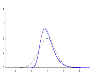
Fig. 1: Density plots of the estimated exact standardized distribution of $t_{\mathcal{U}}$ (red line), the standard Gaussian distribution (black line) and three bootstrap approximations (blue lines). Left panel, $T$=50 ($h=0.2$), right panel $T$=500 ($h=0.04$).

We next investigate the finite sample size and power behavior of the bootstrap studentized test under the aforementioned variety of process parameters and three different sample sizes, $T=50$, $T=100$ and $T=200$. The results obtained are shown in Table 1. As it is evident from this table, the bootstrap studentized test shows a very good empirical size and power behaviour even in the case of $T=50$ observations. In particular, the empirical sizes are close to the nominal ones and the empirical power of the test increases to one as the deviations from the null become larger (i.e., larger values of $a_{2}$) and/or the sample size increases.

Table 1: Empirical size and power of the bootstrap studentized test for functional time series generated according to models (10) and (11).

			b=0.2				b=0.3
$T$	$a_{2}$	$\alpha=0.01$	$\alpha=0.05$	$\alpha=0.10$		$\alpha=0.01$	$\alpha=0.05$	$\alpha=0.10$
50	0.0	0.010	0.048	0.096		0.020	0.058	0.106
	0.2	0.016	0.082	0.158		0.030	0.092	0.164
	0.4	0.062	0.238	0.338		0.048	0.154	0.276
	0.6	0.178	0.390	0.518		0.124	0.334	0.500
	0.8	0.346	0.616	0.736		0.258	0.502	0.670
	1.0	0.488	0.768	0.872		0.464	0.728	0.840
			b=0.1				b=0.2
	$a_{2}$	$\alpha=0.01$	$\alpha=0.05$	$\alpha=0.10$		$\alpha=0.01$	$\alpha=0.05$	$\alpha=0.10$
100	0.0	0.018	0.050	0.092		0.008	0.046	0.080
	0.2	0.028	0.112	0.210		0.028	0.112	0.196
	0.4	0.138	0.328	0.472		0.122	0.344	0.470
	0.6	0.382	0.652	0.764		0.374	0.622	0.766
	0.8	0.650	0.858	0.922		0.624	0.836	0.922
	1.0	0.872	0.968	0.984		0.874	0.966	0.990
			b=0.06				b=0.1
	$a_{2}$	$\alpha=0.01$	$\alpha=0.05$	$\alpha=0.10$		$\alpha=0.01$	$\alpha=0.05$	$\alpha=0.10$
200	0.0	0.014	0.042	0.088		0.004	0.044	0.100
	0.2	0.046	0.154	0.272		0.056	0.164	0.290
	0.4	0.298	0.576	0.698		0.364	0.620	0.760
	0.6	0.708	0.910	0.956		0.788	0.956	0.978
	0.8	0.924	0.992	0.998		0.960	0.996	0.998
	1.0	0.992	1.000	1.000		1.000	1.000	1.000

5.3 A Real-Life Data Example

We applied the bootstrap studentized test to a data set consisting of temperature measurements recorded in Nicosia, Cyprus, for the winter period, December 2006 to beginning of March 2007 and for the summer period, June 2007 to end of August 2007. It is well-known that the mean temperatures during winter periods are smaller than those of summer periods. Our aim is to test whether there is also a significant difference in the autocovariance structure of the winter and summer periods. The data consists of two samples of curves $\{(X_{t},Y_{t}),\;t\in\{1,\ldots,92\}\}$, where $X_{t}$ represents the temperature of day $t$ for Dec2006-Jan2007-Feb2007-March2007 and $Y_{t}$ for Jun2007-Jul2007-Aug2007. More precisely, $X_{1}$ represents the temperature of the 1st of December 2006 and $X_{92}$ the temperature of the 2nd of March 2007, whereas $Y_{1}$ represents the temperature of the 1st of June 2007 and $Y_{92}$ the temperature of the 31st of August 2007. The temperature recordings were taken in $15$ minutes intervals, i.e., there are $k=96$ temperature measurements for each day for a total of $T=92$ days in both groups. These measurements were transformed into functional objects using the Fourier basis with 21 basis functions. All curves were rescaled in order to be defined in the unit interval. Fig. 2 shows the centered temperature curves of the winter and summer periods, i.e., the curves in each group are transformed by subtracting the corresponding group sample mean functions.

Using the cross-validation algorithm described in Section 5.1, the bandwidth chosen is equal to $b_{CV}=0.075$ and the corresponding $p$-value of the bootstrap based studentized test is equal to 0.030 (based on $B=10,000$ bootstrap replications), leading to a rejection of the null hypothesis for almost all commonly used $\alpha$-levels. This implies that the dependence properties, as measured by autocovariances, of the temperature measurements of the winter period differ significantly from those of the summer period.

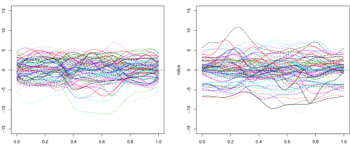
Fig. 2: Centered temperature curves of winter period (left panel) and of summer period (right panel). There are 92 centered curves in each period, rescaled in order to be defined in the unit interval.

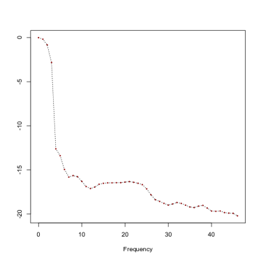
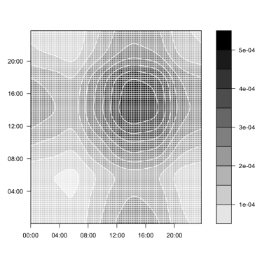
Fig. 3: (a) Plot of $\widehat{Q}_{T,\lambda_{j}}$ (vertical axes, log-scale) against the frequencies $\lambda_{j}$, ${j\in\{0,1,\ldots,N\}}$ (horizontal axes), for the temperature data, using the bandwidth $b=b_{CV}$=0.075. (b) Plot of the difference $\widehat{D}_{T}(\sigma_{r},\tau_{l})$ between the estimated spectral density kernels using the same bandwidth for the values $(\sigma_{r},\tau_{l})$, with $(r,l)\in\{1,\ldots,96\}\times\{1,\ldots,96\}$.

In order to understand the reasons leading to this rejection, we decompose the standardized test $t_{\mathcal{U}}$ after ignoring the centering sequence $b^{-1/2}\widehat{\mu}_{0}$ and approximating the integral of the (squared) Hilbert-Schmidt norm by the corresponding Riemann sum over the Fourier frequencies $\lambda_{j}=2\pi j/T$, as follows:

$$\sqrt{b}T\,\mathcal{U}_{T}\Big{/}\widehat{\theta}_{0} \approx 2\pi\sqrt{b}\sum_{\begin{subarray}{c}j=-N\\ j\neq 0\end{subarray}}^{N}\|\widehat{\mathcal{F}}_{X,\lambda_{j}}-\widehat{\mathcal{F}}_{Y,\lambda_{j}}\|^{2}_{HS}\Big{/}\widehat{\theta}_{0}=\sum_{\begin{subarray}{c}j=-N\\ j\neq 0\end{subarray}}^{N}\widehat{Q}_{T,\lambda_{j}},$$ (12)

where

$$\widehat{Q}_{T,\lambda_{j}}=2\pi\sqrt{b}\,\|\widehat{\mathcal{F}}_{X,\lambda_{j}}-\widehat{\mathcal{F}}_{Y,\lambda_{j}}\|^{2}_{HS}\Big{/}\widehat{\theta}_{0}\geq 0.$$

Expression (12) shows the contributions of the differences $\|\widehat{\mathcal{F}}_{X,\lambda_{j}}-\widehat{\mathcal{F}}_{Y,\lambda_{j}}\|^{2}_{HS}$ for each frequency $\lambda_{j}$ to the total value of the test statistic $\mathcal{U}_{T}$. Large values of $\widehat{Q}_{T,\lambda_{j}}$ pinpoint, therefore, to frequency regions from which large contributions to the test statistic $\mathcal{U}_{T}$ occur. A plot of the estimated quantities $\widehat{Q}_{T,\lambda_{j}}$ against the frequencies $\lambda_{j}$, $j\in\{0,\ldots,N\}$, is, therefore, very informative in identifying frequency regions where differences between the two spectral density operators are large and is very helpful for interpreting the results of the testing procedure.

Complementary to the decomposition $\widehat{Q}_{T,\lambda_{j}}$ of the test statistic ${\mathcal{U}}_{T}$, one also can identify the regions in $[0,1]\times[0,1]$ which deliver large contributions to the test statistic and which lead to a rejection of the null hypothesis. In particular, the test statistic also can be written as

$$\widehat{Q}_{T,\lambda_{j}}\approx\sum_{r=1}^{T}\sum_{l=1}^{T}\widehat{D}^{2}_{T}(\sigma_{r},\tau_{l}),\ \ \widehat{D}_{T}^{2}(\sigma,\tau)=\frac{2\pi\sqrt{b}}{T^{2}}\sum_{\begin{subarray}{c}j=-N\\ j\neq 0\end{subarray}}^{N}\big{|}\widehat{f}_{X,\lambda_{j}}(\sigma,\tau)-\widehat{f}_{Y,\lambda_{j}}(\sigma,\tau)\big{|}^{2}\Big{/}\widehat{\theta}_{0}.$$

Notice that $\widehat{D}_{T}^{2}(\sigma_{r},\tau_{l})$ shows the contribution of the differences between the estimated spectral density kernels (averaged over all Fourier frequencies) at the points $(\sigma_{r},\tau_{l})\in[0,1]\times[0,1]$ to the test statistic ${\mathcal{U}}_{T}$. Large values of $D^{2}_{T}(\sigma_{r},\tau_{l})$ pinpoint to points $(\sigma_{r},\tau_{l})\in[0,1]\times[0,1]$ where large differences (averaged over all frequencies) between the corresponding spectral density kernels occur. Combined with the frequency decomposition $Q_{T,\lambda_{j}}$, the decomposition $D_{T}(\sigma_{r},\tau_{l})$ may further help in better understanding the test results.

Fig. 3(a) shows for the real-life temperature data example considered the plot of $\widehat{Q}_{T,\lambda_{j}}$ at a log-scale. Fig. 3(b) shows, for the same data set, a plot of the differences $\widehat{D}_{T}(\sigma_{r},\tau_{l})$. As it can be seen from Fig. 3(a), the large values of the test statistic $\mathcal{U}_{T}$ which leads to a rejection of the null hypothesis, are mainly due to the large differences between the two spectral density operators at the low frequency region. That is, differences in the long term periodicities between the winter and the summer temperature curves seem to be the main reason for rejecting the null hypothesis. Fig. 3(b) shows that the main differences between the spectral density kernels of the two functional time series, occur in the afternoon period and, more specifically, between the hours 12.00 to 4.00 p.m. The differencies of the (averaged) spectral density kernels, for values of $\tau$ and $\sigma$ within this time frame, seem to be the largest. These findings are probably due to the fact that in Cyprus, compared to the rather day-long stable weather conditions of the summer period, the weather conditions in the winter period are more volatile, change gradually during the day and reach their peak in the afternoon.

Appendix: Auxiliary Results and Proofs

First, we introduce some notation that will be used throughout our proofs. $\|\cdot\|_{2}$ denotes the norm of $L^{2}$, $\|\cdot\|_{\mathcal{N}}$ the nuclear norm of an operator $T$, $T^{*}$ is the adjoint operator and $\langle\cdot,\cdot\rangle_{HS}$ the inner product on the space of Hilbert-Schmidt operators; see the Supplementary Material for more details. Furthermore, we write $A(e^{-i\lambda})=\sum_{j\in{\mathbb{Z}}}A_{j}e^{-ij\lambda}$ with the operators $A_{j}$ defined as in Assumption 1. The periodogram operators of the innovations time series $\varepsilon_{t}$ and $e_{t}$, $t=1,\ldots,n$, at frequency $\lambda$, $I_{\varepsilon,\lambda}$ and $I_{e,\lambda}$, respectively, are defined as the integral operators induced by right integration of

$$\widehat{p}_{\varepsilon,\lambda}(\sigma,\tau) =\frac{1}{2\pi T}\sum_{s_{1},s_{2}=1}^{T}\varepsilon_{s_{1}}(\sigma)\varepsilon_{s_{2}}(\tau)\,\exp(-i\lambda(s_{1}-s_{2})),$$ (13)

$$\widehat{p}_{e,\lambda}(\sigma,\tau) =\frac{1}{2\pi T}\sum_{s_{1},s_{2}=1}^{T}e_{s_{1}}(\sigma)e_{s_{2}}(\tau)\,\exp(-i\lambda(s_{1}-s_{2})).$$

The centered counterparts are denoted by $I_{\varepsilon,\lambda}^{c}$ and $I_{e,\lambda}^{c}$. Finally, define

$$Q_{X,\lambda}^{c}:=A(e^{-i\lambda})I^{c}_{\varepsilon,\lambda}A(e^{-i\lambda})^{*},\ \ Q_{Y,\lambda}^{c}:=B(e^{-i\lambda})I^{c}_{e,\lambda}B(e^{-i\lambda})^{*}.$$

Here, $ST$ denotes the composition $S(T(\cdot))$ of the operators $S$ and $T$.

Proof of Lemma 1. The assertions of the lemma are immediate consequences of Proposition 2.1 in Panaretos and Tavakoli [22] if $\sum_{t\in{\mathbb{Z}}}\|\mathcal{R}_{X,t}\|_{\mathcal{N}}<\infty$ and $\sum_{t\in{\mathbb{Z}}}\|r_{X,t}\|_{2}<\infty$ and similar results for the process $(Y_{t})_{t\in{\mathbb{Z}}}$ hold true. The first inequality follows from expression (1.4) of the supplement. For the second result, use the expression ${\mathcal{R}}_{X,t}=\sum_{j\in{\mathbb{Z}}}A_{j+t}C_{\varepsilon}A^{\ast}_{j}$, see the Supplement Material, and get $\sum_{t\in{\mathbb{Z}}}\|r_{X,t}\|_{2}=\sum_{t\in{\mathbb{Z}}}\|\mathcal{R}_{X,t}\|_{HS}\leq\sum_{t\in{\mathbb{Z}}}\sum_{j\in{\mathbb{Z}}}\|A_{j+t}\|_{\mathcal{L}}\,\|C_{\varepsilon}\|_{HS}\,\|A_{j}\|_{\mathcal{L}}$, which is finite under Assumption 1.

The proof of Theorem 1 uses the following two lemmas, the proofs of which are given in the Supplementary Material.

Lemma 2.

Suppose that the assumptions of Theorem 1 hold true. Then

$$\sqrt{b}T\,M_{T,0}-b^{-1/2}\,\mu_{0}=o_{P}(1),$$

where

$$M_{T,0} =\int_{-\pi}^{\pi}\frac{1}{b^{2}T^{2}}\sum_{t=-N}^{N}W^{2}\left(\frac{\lambda-\lambda_{t}}{b}\right)\left\|Q_{X,\lambda_{t}}^{c}-Q_{Y,\lambda_{t}}^{c}\right\|_{HS}^{2}d\lambda\,.$$ (14)

Lemma 3.

Suppose that the assumptions of Theorem 1 hold true. Then,

$${\rm var}(\sqrt{b}T\,L_{T,0})\mathop{\longrightarrow}\limits_{T\to\infty}\theta_{0}^{2}$$

for $\theta_{0}$ defined in Theorem 1, where

$$L_{T,0} =\frac{1}{b^{2}T^{2}}\int_{-\pi}^{\pi}\int_{0}^{1}\int_{0}^{1}\sum_{t_{1},t_{2}=-N,\,t_{1}\neq t_{2}}^{N}\,W\left(\frac{\lambda-\lambda_{t_{1}}}{b}\right)\,W\left(\frac{\lambda-\lambda_{t_{2}}}{b}\right)\,d\lambda$$ (15)

$$\quad\times\Big{\langle}Q_{X,\lambda_{t_{1}}}^{c}-Q_{Y,\lambda_{t_{1}}}^{c}\;,Q_{X,\lambda_{t_{2}}}^{c}-Q_{Y,\lambda_{t_{2}}}^{c}\Big{\rangle}_{HS}.$$

Proof of Theorem 1. From Theorem 1.2 of the Supplementary Material we obtain

$$I_{X,\lambda}=A(e^{-i\lambda})I_{\varepsilon,\lambda}A(e^{-i\lambda})^{*}+R_{T,\lambda}\quad\text{with}\quad\sup_{\lambda\in\{2\pi t/T|t=-N,\dots,N\}}{\rm E}\|R_{T,\lambda}\|_{HS}^{2}=O(T^{-1}).$$

This gives

$$\sqrt{b}T\,\mathcal{U}_{T} =\sqrt{b}T\int_{-\pi}^{\pi}\left\|\frac{1}{bT}\sum_{t=-N}^{N}W\left(\frac{\lambda-\lambda_{t}}{b}\right)\left[A(e^{-i\lambda_{t}})I_{\varepsilon,\lambda_{t}}A(e^{-i\lambda_{t}})^{*}-B(e^{-i\lambda_{t}})I_{e,\lambda_{t}}B(e^{-i\lambda_{t}})^{*}\right]\right\|_{HS}^{2}d\lambda$$

$$\quad\;+O_{P}(b^{1/4})=:\sqrt{b}T\,U_{T,0}+o_{P}(1)$$ (16)

if we can show that $\sqrt{b}T\,U_{T,0}=O_{P}(1)$. To this end, first note that under $\mathcal{H}_{0}$ $\mathcal{F}_{X}=\mathcal{F}_{Y}$. Now, it follows from (1.5) in the Supplementary Material that

$$\frac{1}{2\pi}\,A(e^{-i\lambda_{t}})\,C_{\varepsilon}\,A(e^{-i\lambda_{t}})^{*}=\mathcal{F}_{X}=\mathcal{F}_{Y}=\frac{1}{2\pi}\,B(e^{-i\lambda_{t}})\,C_{e}\,B(e^{-i\lambda_{t}})^{*}.$$

Additionally, we have ${\rm E}\widehat{p}_{\varepsilon,\lambda}(\sigma,\tau)=c_{\varepsilon}(\sigma,\tau)/(2\pi)$ and ${\rm E}\widehat{p}_{e,\lambda}(\sigma,\tau)=c_{e}(\sigma,\tau)/(2\pi)$ in $L^{2}$ for the i.i.d. noises. Combining both facts, we can rewrite $U_{T,0}$ as

$$U_{T,0}=\int_{-\pi}^{\pi}\left\|\frac{1}{bT}\sum_{t=-N}^{N}W\left(\frac{\lambda-\lambda_{t}}{b}\right)\left[A(e^{-i\lambda_{t}})I^{c}_{\varepsilon,\lambda_{t}}A(e^{-i\lambda_{t}})^{*}-B(e^{-i\lambda_{t}})I^{c}_{e,\lambda_{t}}B(e^{-i\lambda_{t}})^{*}\right]\right\|_{HS}^{2}d\lambda.$$ (17)

We can further split up $U_{T,0}=M_{T,0}+L_{T,0}$ where $M_{T,0}$ and $L_{T,0}$ are defined as in Lemma 2 and Lemma 3, respectively. In view of Lemma 2, it remains to show that $\sqrt{b}TL_{T,0}\stackrel{{\scriptstyle d}}{{\longrightarrow}}Z.$ To this end, we abbreviate

$$w_{t_{1},t_{2},T}=\frac{1}{b^{3/2}T}\int_{-\pi}^{\pi}W\left(\frac{\lambda-\lambda_{t_{1}}}{b}\right)\,W\left(\frac{\lambda-\lambda_{t_{2}}}{b}\right)\,d\lambda$$

and use the Karhunen-Lóeve expansion for the Gaussian innovations $\varepsilon_{t}$ and $e_{t}$. In particular, we have

$$\varepsilon_{s}(\sigma)=\sum_{l}\xi_{l}^{(s)}\varphi_{l}(\sigma),\quad s\in{\mathbb{Z}},~{}\sigma\in[0,1],$$

where $\varphi_{l}\in L^{2}$, $l\in{\mathbb{N}}$, denotes the set of orthonormal eigenfunctions of the operator $C_{\varepsilon}$ and the random variables $\xi_{l}^{(s)}=\int_{0}^{1}\varepsilon_{s}(\sigma)\,\varphi_{l}(\sigma)\,d\sigma$ are centered normal and satisfy ${\rm cov}(\xi_{l_{1}}^{(s)},\xi_{l_{2}}^{(s)})=0$ for $l_{1}\neq l_{2}.$ Notice that the above expression for $\varepsilon_{s}(\sigma)$ is valid in $L^{2}$-sense and that Fubini’s theorem gives ${\rm cov}(\xi_{l_{1}}^{(s_{1})},\xi_{l_{2}}^{(s_{2})})=0$ for $s_{1}\neq s_{2}$. A similar expansion holds true for $e_{s}$ with a possibly different set of othonormal eigenfunctions $(\phi_{l})_{l\in{\mathbb{N}}}$ instead of $(\varphi_{l})_{l\in{\mathbb{N}}}$. Now, we define approximating periodogram operators $I_{\varepsilon,\lambda_{t}}^{c,K},\;K\in{\mathbb{N}}$, with kernels

$$\widehat{p}_{\varepsilon,\lambda_{t}}^{c,K}=\sum_{l_{1},l_{2}=1}^{K}\varphi_{l_{1}}\varphi_{l_{2}}\frac{1}{2\pi T}\sum_{s_{1},s_{2}}e^{i\lambda_{t}(s_{1}-s_{2})}\,[\xi_{l_{1}}^{(s_{1})}\xi_{l_{2}}^{(s_{2})}-E(\xi_{l_{1}}^{(s_{1})}\xi_{l_{2}}^{(s_{2})})]$$

and similarly for $I_{e,\lambda_{t}}^{c,K}$. Moreover, define

$$Q_{X,\lambda}^{c,K}:=A(e^{-i\lambda})I^{c,K}_{\varepsilon,\lambda}A(e^{-i\lambda})^{*}\quad\text{and}\quad Q_{Y,\lambda}^{c,K}:=B(e^{-i\lambda})I^{c,K}_{e,\lambda}B(e^{-i\lambda})^{*}.$$

Then, we can introduce

$$\sqrt{b}T\,L_{T,0}^{(K)} =\sum_{t_{1},t_{2}=-N,\,t_{1}\neq t_{2}}^{N}\,w_{t_{1},t_{2},T}\;\Big{\langle}Q_{X,\lambda_{t_{1}}}^{c,K}-Q_{Y,\lambda_{t_{1}}}^{c,K}\;,Q_{X,\lambda_{t_{2}}}^{c,K}-Q_{Y,\lambda_{t_{2}}}^{c,K}\Big{\rangle}_{HS}=:\sum_{t_{1},t_{2}=-N,t_{1}\neq t_{2}}^{N}H_{t_{1},t_{2},T}.$$

From this, we get

$$\lim_{K\to\infty}\limsup_{T\to\infty}{\rm E}(\sqrt{b}T(\,L_{T,0}-\,L_{T,0}^{(K)}))^{2}=0.$$ (18)

To this end, first note that under Gaussianity $|{\rm E}L_{T,0}|+|{\rm E}L_{T,0}^{(K)}|=o(1)$ for any $K$ due to independence of the spectral density operators at different frequencies $|t_{1}|\neq|t_{2}|$. Thus, it suffices to investigate ${\rm var}(\sqrt{b}T(\,L_{T,0}-\,L_{T,0}^{(K)}))$. With the same arguments as in the proof of Lemma 3 it suffices to show that

$$\sup_{|t_{1}|\neq|t_{2}|,|s_{1}|\neq|s_{2}|}{\rm cov} \Big{(}\Big{\langle}Q_{X,\lambda_{t_{1}}}^{c}-Q_{Y,\lambda_{t_{1}}}^{c}\;,Q_{X,\lambda_{t_{2}}}^{c}-Q_{Y,\lambda_{t_{2}}}^{c}\Big{\rangle}_{HS}-\Big{\langle}Q_{X,\lambda_{t_{1}}}^{c,K}-Q_{Y,\lambda_{t_{1}}}^{c,K}\;,Q_{X,\lambda_{t_{2}}}^{c,K}-Q_{Y,\lambda_{t_{2}}}^{c,K}\Big{\rangle}_{HS},$$

$$\Big{\langle}Q_{X,\lambda_{s_{1}}}^{c}-Q_{Y,\lambda_{s_{1}}}^{c}\;,Q_{X,\lambda_{s_{2}}}^{c}-Q_{Y,\lambda_{s_{2}}}^{c}\Big{\rangle}_{HS}-\Big{\langle}Q_{X,\lambda_{s_{1}}}^{c,K}-Q_{Y,\lambda_{s_{1}}}^{c,K}\;,Q_{X,\lambda_{s_{2}}}^{c,K}-Q_{Y,\lambda_{s_{2}}}^{c,K}\Big{\rangle}_{HS}\Big{)}$$

converges to zero as $K\to\infty$ in the cases $t_{1}=\pm s_{1},t_{2}=\pm s_{2}$ and $t_{1}=\pm s_{2},t_{2}=\pm s_{1}$. Exemplarily we only investigate

$$\sup_{|t_{1}|\neq|t_{2}|}{\rm cov} \Big{(}\Big{\langle}Q_{X,\lambda_{t_{1}}}^{c}\;,Q_{X,\lambda_{t_{2}}}^{c}\Big{\rangle}_{HS}-\Big{\langle}Q_{X,\lambda_{t_{1}}}^{c,K}\;,Q_{X,\lambda_{t_{2}}}^{c,K}\Big{\rangle}_{HS},$$

$$\Big{\langle}Q_{X,\lambda_{t_{1}}}^{c}\;,Q_{X,\lambda_{t_{2}}}^{c}\Big{\rangle}_{HS}-\Big{\langle}Q_{X,\lambda_{t_{1}}}^{c,K}\;,Q_{X,\lambda_{t_{2}}}^{c,K}\Big{\rangle}_{HS}\Big{)}$$

in detail. With similar arguments as in Lemma 3 it can be shown that all remaining summands vanish, too. Using symmetry arguments and adding zeros, it suffices to consider

$$\sup_{|t_{1}|\neq|t_{2}|}{\rm cov} \Big{(}\Big{\langle}Q_{X,\lambda_{t_{1}}}^{c}-Q_{X,\lambda_{t_{1}}}^{c,K}\;,Q_{X,\lambda_{t_{2}}}^{c}\Big{\rangle}_{HS},\Big{\langle}Q_{X,\lambda_{t_{1}}}^{c}\;,Q_{X,\lambda_{t_{2}}}^{c}\Big{\rangle}_{HS}\Big{)}$$ (19)

and similar terms. To this end, let

$$C_{\epsilon}^{(K)}={\rm E}\left[\left(\sum_{l=1}^{K}\xi_{l}^{(0)}\varphi_{l}\right)\otimes\left(\sum_{l=1}^{K}\xi_{l}^{(0)}\varphi_{l}\right)\right].$$

In analogy to the proof of Lemma 3, (19) can be bounded from above by

$$\sup_{|t_{1}|\neq|t_{2}|}\|A(e^{-i\lambda_{t_{1}}})\|_{\mathcal{L}}^{4}\,\left\|{\rm E}\left([I_{\varepsilon,\lambda_{t_{1}}}^{c}-I_{\varepsilon,\lambda_{t_{1}}}^{c,K}]\otimes I_{\varepsilon,\lambda_{t_{1}}}^{c}\right)\right\|_{HS}\,\|\mathcal{F}_{X,\lambda_{t_{2}}}\|_{HS}^{2}\leq\mathcal{K}\,\|C_{\varepsilon}-C_{\epsilon}^{(K)}\|_{HS}+o(1)$$

for some finite constant $\mathcal{K}$, where the last inequality can be obtained similarly to Lemma 1.7 and Theorem 1.3 in the supplement. Mercer’s Theorem finally gives $\|C_{\varepsilon}-C_{\epsilon}^{(K)}\|_{HS}\to 0$ as $K\to\infty$. We aim at applying a CLT of de Jong [6] for weighted $U$-statistics of independent random vectors. To this end, we rewrite

$$\sqrt{b}T\,L_{T,0}^{(K)}=\sum_{t_{1},t_{2}=1,t_{1}\neq t_{2}}^{N}\widetilde{H}_{t_{1},t_{2},T}+\sum_{t=-N}^{N}[H_{t,0,T}+H_{0,t,T}]+\sum_{t_{1}=-N}^{N}H_{t_{1},-t_{1},T}-2H_{0,0,T},$$

where

$$\widetilde{H}_{t_{1},t_{2}}=H_{t_{1},t_{2},T}+H_{-t_{1},t_{2},T}+H_{t_{1},-t_{2},T}+H_{-t_{1},-t_{2},T}.$$

Straightforward calculations yield that

$$\sum_{t=-N}^{N}[H_{t,0,T}+H_{0,t,T}]+\sum_{t_{1}=-N}^{N}H_{t_{1},-t_{1},T}-2H_{0,0,T}=o_{P}(1)$$

in $L^{2}$. Now, we apply Theorem 2.1 of de Jong [6] to

$$\widetilde{W}_{T}=\sum_{\begin{subarray}{c}t_{1},t_{2}=1\\ t_{1}\neq t_{2}\end{subarray}}^{N}\,\widetilde{H}_{t_{1},t_{2}}=\sum_{\begin{subarray}{c}t_{1},t_{2}=1\\ t_{1}\neq t_{2}\end{subarray}}^{N}\,\widetilde{H}_{t_{1},t_{2}}(\mathbb{X}_{t_{1}},\mathbb{X}_{t_{2}}),$$

where $H_{t_{1},t_{2}}$ is a Borel function and

$$\mathbb{X}_{t}=\frac{1}{\sqrt{2\pi T}}\sum_{s=1}^{T}(\xi_{s}^{(1)}\cos(\lambda_{t}s),\xi_{s}^{(1)}\sin(\lambda_{t}s),\ldots,\xi_{s}^{(K)}\cos(\lambda_{t}s),\xi_{s}^{(K)}\sin(\lambda_{t}s))^{\prime}$$

in their notation. First, note that the assumption of Gaussian innovations implies independence of $\mathbb{X}_{1},\dots,\mathbb{X}_{N}$. Moreover, this yields ${\rm E}(\widetilde{H}_{t_{1},t_{2}}\mid\mathbb{X}_{t_{1}})={\rm E}(\widetilde{H}_{t_{1},t_{2}}\mid\mathbb{X}_{t_{2}})=0~{}a.s.$ for $t_{1}\neq t_{2}$ which implies that $\widetilde{W}_{T}$ is clean (see Definition 2.1 in de Jong [6]). It remains to check conditions (a) and (b) of Theorem 2.1 of de Jong [6]. Similar to Lemma 3 we obtain that ${\rm var}(\widetilde{W}_{T})$ converges to the finite constant

$$\theta_{K}:=\frac{4}{\pi^{2}}\int_{-2\pi}^{2\pi}\left\{\int_{-\pi}^{\pi}W(u)W(u-x)\,du\right\}^{2}dx\,\int_{-\pi}^{\pi}\|A(e^{-i\lambda_{t_{1}}})\,E[I_{\varepsilon,\lambda_{t_{1}}}^{c,K}]\,A(e^{-i\lambda_{t_{1}}})^{*}\|_{HS}^{4}\,d\lambda.$$

Subsequently, we only consider the non-trivial case of $\theta_{L}>0$. For condition (a), it remains to verify that

$$\max_{t_{1}\in\{1,\dots,N\}}\sum_{\begin{subarray}{c}t_{2}=1\\ t_{2}\neq t_{1}\end{subarray}}^{N}{\rm var}\left(\widetilde{H}_{t_{1},t_{2}}\right)=o(1).$$

This is an immediate consequence of ${\rm var}(H_{t_{1},t_{2}})=0$ for $|t_{1}-t_{2}|>bT$ and

$${\rm var}(H_{t_{1},t_{2}})=O\left(\frac{1}{b\,T^{2}}\right)\,=o\left(\frac{1}{bT}\right)$$

for $|t_{1}-t_{2}|\leq bT$. Finally, we have to check assumption (b) of Theorem 2.1 of de Jong [6], i.e.,

$${\rm E}\widetilde{W}_{T}^{4}\mathop{\longrightarrow}\limits_{T\to\infty}3\theta_{K}^{2}.$$

To this end, we argue that ${\rm E}\widetilde{W}_{T}^{2}\mathop{\longrightarrow}\limits_{T\to\infty}\theta_{K}^{2}$ and that the forth-order cumulant of $\widetilde{W}_{T}$ vanishes asymptotically due to the independence of the periodograms at different Fourier frequencies. Finally, note that $\theta_{K}\to\theta_{0}$ as $K\to\infty$ which finishes the proof by Proposition 6.3.9 in Brockwell and Davis [4].

Proof of Theorem 2. Recall first that in the following calculations all indices in the sums considered, run in the set $\{-N,-N+1,\ldots,-1,1,\ldots,N-1,N\}$, where $N=[(T-1)/2]$. Let $\{v_{j},j\in{\mathbb{N}}\}$ be an orthonormal basis of $L_{\mathbb{C}}^{2}:=L_{\mathbb{C}}^{2}([0,1],\mu)$ and recall that $\{v_{i}\otimes v_{j},i,j\in{\mathbb{N}}\}$ is an orthonormal basis of the Hilbert space $HS(L_{\mathbb{C}}^{2})$. The bootstrap test statistic

$$\mathcal{U}^{\ast}_{T}=\frac{2\pi}{T}\sum_{l=-N}^{N}\|\widehat{\mathcal{F}}_{X,\lambda_{t}}^{\ast}-\widehat{\mathcal{F}}_{Y,\lambda_{t}}^{\ast}\|^{2}_{HS}$$ (20)

can then be decomposed as

$$\mathcal{U}^{\ast}_{T} =\frac{2\pi}{T^{3}b^{2}}\sum_{t_{1}=-N}^{N}\sum_{t_{2}=-N}^{N}\sum_{l=-N}^{N}W\Big{(}\frac{\lambda_{l}-\lambda_{t_{1}}}{b}\Big{)}W\Big{(}\frac{\lambda_{l}-\lambda_{t_{2}}}{b}\Big{)}\langle I^{\ast}_{X,\lambda_{t_{1}}}-I^{\ast}_{Y,\lambda_{t_{1}}},I^{\ast}_{X,\lambda_{t_{2}}}-I^{\ast}_{Y,\lambda_{t_{2}}}\rangle_{HS}$$

$$=\frac{2\pi}{T^{3}b^{2}}\sum_{t=-N}^{N}\sum_{l=-N}^{N}W^{2}\Big{(}\frac{\lambda_{l}-\lambda_{t}}{b}\Big{)}\|I^{\ast}_{X,\lambda_{t}}-I^{\ast}_{Y,\lambda_{t}}\|_{HS}^{2}$$

$$\ \ \ \ +\frac{2\pi}{T^{3}b^{2}}\sum_{\begin{subarray}{c}t_{1},t_{2}=-N\\ t_{|}\neq t_{2}\end{subarray}}^{N}W\Big{(}\frac{\lambda_{l}-\lambda_{t_{1}}}{b}\Big{)}W\Big{(}\frac{\lambda_{l}-\lambda_{t_{2}}}{b}\Big{)}\langle I^{\ast}_{X,\lambda_{t_{1}}}-I^{\ast}_{Y,\lambda_{t_{1}}},I^{\ast}_{X,\lambda_{t_{2}}}-I^{\ast}_{Y,\lambda_{t_{2}}}\rangle_{HS}\ :=M^{\ast}_{T}+L^{\ast}_{T},$$

with an obvious notation for $M^{\ast}_{T}$ and $L^{\ast}_{T}$. In the following we use the notation

$$D^{*}_{t}(j_{1},j_{2}):=\langle I^{\ast}_{X,\lambda_{t}}-I^{\ast}_{Y,\lambda_{t}},v_{j_{1}}\otimes v_{j_{2}}\rangle=\langle J^{\ast}_{X,\lambda_{t}},v_{j_{1}}\rangle\langle v_{j_{2}},\overline{J}^{\ast}_{X,\lambda_{t}}\rangle-\langle J^{\ast}_{Y,\lambda_{t}},v_{j_{1}}\rangle\langle v_{j_{2}},\overline{J}^{\ast}_{Y,\lambda_{t}}\rangle,$$

and the expansion

$$I^{\ast}_{X,\lambda_{t}}-I^{\ast}_{Y,\lambda_{t}} =J^{\ast}_{X,\lambda_{t}}\otimes\overline{J}^{\ast}_{X,\lambda_{t}}-J^{\ast}_{Y,\lambda_{t}}\otimes\overline{J}^{\ast}_{Y,\lambda_{t}}=\sum_{j_{1}=1}^{\infty}\sum_{j_{2}=1}^{\infty}D_{t}^{{*}}(j_{1},j_{2})(v_{j_{1}}\otimes v_{j_{2}}).$$

Notice that $\langle J^{\ast}_{X,\lambda_{t}},v_{j}\rangle$ is for every $j\in{\mathbb{N}}$, a complex Gaussian random variable. We show that

$$\sqrt{b}TM_{T}^{\ast}\,-\,b^{-1/2}\,\widetilde{\mu}_{0}\stackrel{{\scriptstyle P}}{{\rightarrow}}0,$$ (21)

and

$$\sqrt{b}TL_{T}^{\ast}\stackrel{{\scriptstyle d}}{{\rightarrow}}\mathcal{N}(0,\widetilde{\theta}_{0}^{2}).$$ (22)

Let $I^{\ast^{C}}_{X,\lambda_{t}}=I_{X,\lambda_{t}}-\widehat{\mathcal{F}}_{\lambda_{t}}$ and similarly for $I^{\ast^{C}}_{Y,\lambda_{t}}$. Verify that

$${\rm E}^{\star}\langle I^{\ast^{C}}_{X,\lambda_{t}},v_{j_{1}}\otimes v_{j_{2}}\rangle_{HS}\langle I^{\ast^{C}}_{X,\lambda_{t}},v_{j_{1}}\otimes v_{j_{2}}\rangle_{HS} ={\rm E}^{\star}\langle I^{\ast^{C}}_{X,\lambda_{t}}(v_{j_{2}}),v_{j_{1}}\rangle\langle I^{\ast^{C}}_{X,\lambda_{t}}(v_{j_{2}}),v_{j_{1}}\rangle$$

$$=\langle{\rm E}^{\star}I^{\ast^{C}}_{X,\lambda_{t}}(v_{j_{2}})\otimes\overline{I}^{\ast^{C}}_{X,\lambda_{t}}(v_{j_{1}}),v_{j_{1}}\otimes v_{j_{2}}\rangle_{HS}$$

$$=\langle\widehat{\mathcal{F}}_{\lambda_{t}}(v_{j_{1}})\otimes\widehat{\mathcal{F}}_{\lambda_{t}}(v_{j_{2}}),v_{j_{1}}\otimes v_{j_{2}}\rangle_{HS}$$

$$=\langle\widehat{\mathcal{F}}_{\lambda_{t}}(v_{j_{1}}),v_{j_{1}}\rangle\langle v_{j_{2}},\widehat{\mathcal{F}}_{\lambda_{t}}(v_{j_{2}})\rangle.$$ (23)

Furthermore,

$${\rm cov}^{\ast}(D^{*}_{t}(j_{1},j_{2}), D^{*}_{t}(r_{1},r_{2}))={\rm E}^{\star}(D^{*}_{t}(j_{1},j_{2})\overline{D}^{*}_{t}(r_{1},r_{2}))$$

$$={\rm E}^{\star}\langle I^{\ast^{C}}_{X,\lambda_{t}},v_{j_{1}}\otimes v_{j_{2}}\rangle_{HS}\langle\overline{I}^{\ast^{C}}_{X,\lambda_{t}},v_{r_{1}}\otimes v_{r_{2}}\rangle_{HS}+{\rm E}^{\star}\langle I^{\ast^{C}}_{Y,\lambda_{t}},v_{j_{1}}\otimes v_{j_{2}}\rangle_{HS}\langle\overline{I}^{\ast^{C}}_{Y,\lambda_{t}},v_{r_{1}}\otimes v_{r_{2}}\rangle_{HS}$$

$$=2\langle\widehat{\mathcal{F}}_{\lambda_{t}}(v_{r_{2}}),v_{j_{1}}\rangle\langle v_{j_{2}},\widehat{\mathcal{F}}_{\lambda_{t}}(v_{r_{1}})\rangle=2\langle\widehat{\mathcal{F}}_{\lambda_{t}}(v_{r_{2}})\otimes\widehat{\mathcal{F}}_{\lambda_{t}}(v_{r_{1}}),v_{j_{1}}\otimes v_{j_{2}}\rangle_{HS},$$ (24)

where the last two equalities follow using the derivations in (Appendix: Auxiliary Results and Proofs).

Consider first (21). Using (Appendix: Auxiliary Results and Proofs), we get

$${\rm E}^{\ast}(\sqrt{b}TM^{\ast}_{T}) =\frac{2\pi}{T^{2}b^{3/2}}\sum_{j_{1},j_{2}=1}^{\infty}\sum_{t=-N}^{N}\sum_{l=-N}^{N}W^{2}\Big{(}\frac{\lambda_{l}-\lambda_{t}}{b}\Big{)}{\rm E}^{\star}\langle I^{\ast^{C}}_{X,\lambda_{t}}-I^{\ast^{C}}_{Y,\lambda_{t}},v_{j_{1}}\otimes v_{j_{2}}\rangle^{2}_{HS}$$

$$=\frac{2\pi}{T^{2}b^{3/2}}\sum_{j_{1},j_{2}=1}^{\infty}\sum_{t=-N}^{N}\sum_{l=-N}^{N}W^{2}\Big{(}\frac{\lambda_{l}-\lambda_{t}}{b}\Big{)}\big{\{}{\rm E}^{\star}\langle I^{\ast^{C}}_{X,\lambda_{t}},v_{j_{1}}\otimes v_{j_{2}}\rangle_{HS}\langle I^{\ast^{C}}_{X,\lambda_{t}},v_{j_{1}}\otimes v_{j_{2}}\rangle_{HS}$$

$$\ \ \ \ \ \ \ \ \ \ +{\rm E}^{\star}\langle I^{\ast^{C}}_{Y,\lambda_{t}},v_{j_{1}}\otimes v_{j_{2}}\rangle_{HS}\langle I^{\ast^{C}}_{Y,\lambda_{t}},v_{j_{1}}\otimes v_{j_{2}}\rangle_{HS}\big{\}}$$

$$=\frac{4\pi}{T^{2}b^{3/2}}\sum_{j_{1},j_{2}=1}^{\infty}\sum_{t=-N}^{N}\sum_{l=-N}^{N}W^{2}\Big{(}\frac{\lambda_{l}-\lambda_{t}}{b}\Big{)}\langle\widehat{\mathcal{F}}_{X,\lambda_{t}}(v_{j_{1}}),v_{j_{1}}\rangle\langle v_{j_{2}},\widehat{\mathcal{F}}_{X,\lambda_{t}}(v_{j_{2}})\rangle$$

$$=\frac{4\pi}{T^{2}b^{3/2}}\sum_{t=-N}^{N}\sum_{l=-N}^{N}W^{2}\big{(}\frac{\lambda_{l}-\lambda_{t}}{b}\big{)}\big{(}\mathrm{trace}(\widehat{\mathcal{F}}_{\lambda_{t}})\big{)}^{2}$$

$$=\frac{4\pi}{T^{2}b^{3/2}}\sum_{t=-N}^{N}\sum_{l=-N}^{N}W^{2}\big{(}\frac{\lambda_{l}-\lambda_{t}}{b}\big{)}\big{(}\mathrm{trace}({\mathcal{F}}_{\lambda_{t}})\big{)}^{2}+o_{P}(1).$$

and, therefore,

$$b^{1/2}{\rm E}^{\ast}(\sqrt{b}TM^{\ast}_{T})=\frac{4\pi}{T^{2}b}\sum_{t=-N}^{N}\sum_{l=-N}^{N}W^{2}\big{(}\frac{\lambda_{l}-\lambda_{t}}{b}\big{)}\big{(}\mathrm{trace}(F_{\lambda_{t}})\big{)}^{2}+o_{P}(1)\stackrel{{\scriptstyle P}}{{\rightarrow}}\widetilde{\mu}_{0}.$$ (25)

Furthermore,

$${\rm var}^{\ast}(\sqrt{b}TM^{\ast}_{T}) =\frac{4\pi^{2}}{T^{4}b^{3}}\sum_{j_{1},j_{2}=1}^{\infty}\sum_{r_{1},r_{2}=1}^{\infty}\sum_{t_{1},t_{2}=-N}^{N}\sum_{l_{1},l_{2}=-N}^{N}W^{2}\Big{(}\frac{\lambda_{l_{1}}-\lambda_{t_{1}}}{b}\Big{)}W^{2}\Big{(}\frac{\lambda_{l_{2}}-\lambda_{t_{2}}}{b}\Big{)}$$

$$\ \ \ \ \times{\rm cov}^{\ast}(D^{\ast}_{{t_{1}}}(j_{1},j_{2}),D^{\ast}_{{t_{2}}}(r_{1},r_{2}))$$

which due to the independence of $D^{\ast}_{{t_{1}}}(j_{1},j_{2})$ and $D^{\ast}_{{t_{2}}}(j_{1},j_{2})$ for $|\lambda_{t_{1}}|\neq|\lambda_{t_{2}}|$, is reduced to four terms with a typical one given by

$$\frac{4\pi^{2}}{T^{4}b^{3}}\sum_{t=1}^{N}\sum_{l_{1},l_{2}=-N}^{N}W^{2}\Big{(}\frac{\lambda_{l_{1}}-\lambda_{t}}{b}\Big{)}W^{2}\Big{(}\frac{\lambda_{l_{2}}-\lambda_{t}}{b}\Big{)}\ \times\sum_{j_{1},j_{2}=1}^{\infty}\sum_{r_{1},r_{2}=1}^{\infty}{\rm cov}^{\ast}(D^{\ast}_{{t}}(j_{1},j_{2}),D^{\ast}_{{t}}(r_{1},r_{2}))$$

and which is easily seen to be of order $O_{P}((Tb)^{-1})$. Similar arguments applied to the other three terms show that they also are asymptotically negligible from which we get that ${\rm var}^{\ast}(\sqrt{b}TM^{\ast}_{T})\stackrel{{\scriptstyle P}}{{\rightarrow}}0$. In view of (25) this implies that $\sqrt{b}TM_{T}^{\ast}\,-\,b^{-1/2}\,\widetilde{\mu}_{0}\stackrel{{\scriptstyle P}}{{\rightarrow}}0$.

Consider next (22). Notice that

$${\rm var}^{\ast}(\sqrt{b}TL^{\ast}_{T})=\frac{4\pi^{2}}{T^{4}b^{3}}\sum_{j_{1},j_{2}=1}^{\infty}\sum_{r_{1},r_{2}=1}^{\infty}\sum_{\begin{subarray}{c}t_{1},t_{2}=-N\\ t_{1}\neq t_{2}\end{subarray}}^{N}\sum_{\begin{subarray}{c}t_{3},t_{4}=-N\\ t_{3}\neq t_{4}\end{subarray}}^{N}\sum_{l_{1},l_{2}=-N}^{N}W\Big{(}\frac{\lambda_{l_{1}}-\lambda_{t_{1}}}{b}\Big{)}W\Big{(}\frac{\lambda_{l_{1}}-\lambda_{t_{2}}}{b}\Big{)}$$

$$\quad\times W\Big{(}\frac{\lambda_{l_{2}}-\lambda_{t_{3}}}{b}\Big{)}W\Big{(}\frac{\lambda_{l_{2}}-\lambda_{t_{4}}}{b}\Big{)}\Big{\{}{\rm E}^{\ast}\big{(}D^{\ast}_{t_{1}}(j_{1},j_{2})\overline{D^{\ast}_{t_{3}}}(r_{1},r_{2})\big{)}{\rm E}^{\ast}\big{(}D^{\ast}_{t_{2}}(j_{1},j_{2})\overline{D^{\ast}_{t_{4}}}(r_{1},r_{2})\big{)}$$

$$+{\rm E}^{\ast}\big{(}D^{\ast}_{t_{1}}(j_{1},j_{2})\overline{D^{\ast}_{t_{4}}}(r_{1},r_{2})\big{)}{\rm E}^{\ast}\big{(}D^{\ast}_{t_{2}}(j_{1},j_{2})\overline{D^{\ast}_{t_{3}}}(r_{1},r_{2})\big{)}+{\rm cum}^{\star}\big{(}D^{\ast}_{t_{1}}(j_{1},j_{2}),\overline{D^{\ast}_{t_{2}}}(j_{1},j_{2}),D^{\ast}_{t_{3}}(r_{1},r_{2}),\overline{D^{\ast}_{t_{4}}}(r_{1},r_{2})\big{)}\Big{\}}$$

$$=V_{1,T}^{\ast}+V_{2,T}^{\ast}+V_{3,T}^{\ast},$$

with an obvious notation for $V_{i,T}^{\ast}$, $i\in\{1,2,3\}$. Since ${\rm E}^{\ast}\big{(}D^{\ast}_{t}(j_{1},j_{2})\overline{D^{\ast}_{s}}(r_{1},r_{2})\big{)}=0$ for $|t|\neq|s|$ we get using (Appendix: Auxiliary Results and Proofs) and $\sum_{j_{1},j_{2}=1}^{\infty}\langle\widehat{\mathcal{F}}_{\lambda_{t_{1}}}(v_{r_{2}})\otimes\widehat{\mathcal{F}}_{\lambda_{t_{1}}}(v_{r_{1}}),v_{j_{1}}\otimes v_{j_{2}}\rangle_{HS}(v_{j_{1}}\otimes v_{j_{2}})=\widehat{\mathcal{F}}_{\lambda_{t_{1}}}(v_{r_{2}})\otimes\widehat{\mathcal{F}}_{\lambda_{t_{1}}}(v_{r_{1}})$, that

$$V_{1,T}^{\ast}=\frac{16\pi^{2}}{T^{4}b^{3}}\sum_{j_{1},j_{2}=1}^{\infty}\sum_{r_{1},r_{2}=1}^{\infty}\sum_{t_{1},t_{2}=-N}^{N}\sum_{l_{1},l_{2}=-N}^{N}W\Big{(}\frac{\lambda_{l_{1}}-\lambda_{t_{1}}}{b}\Big{)}W\Big{(}\frac{\lambda_{l_{2}}-\lambda_{t_{1}}}{b}\Big{)}W\Big{(}\frac{\lambda_{l_{2}}-\lambda_{t_{2}}}{b}\Big{)}W\Big{(}\frac{\lambda_{l_{1}}-\lambda_{t_{2}}}{b}\Big{)}$$

$$\quad\times\langle\widehat{\mathcal{F}}_{\lambda_{t_{1}}}(v_{r_{2}})\otimes\widehat{\mathcal{F}}_{\lambda_{t_{1}}}(v_{r_{1}}),v_{j_{1}}\otimes v_{j_{2}}\rangle_{HS}\langle\widehat{\mathcal{F}}_{\lambda_{t_{2}}}(v_{r_{2}})\otimes\widehat{\mathcal{F}}_{\lambda_{t_{2}}}(v_{r_{1}}),v_{j_{1}}\otimes v_{j_{2}}\rangle_{HS}$$

$$=\frac{16\pi^{2}}{T^{4}b^{3}}\sum_{r_{1},r_{2}=1}^{\infty}\sum_{t_{1},t_{2}=-N}^{N}\sum_{l_{1},l_{2}=-N}^{N}W\Big{(}\frac{\lambda_{l_{1}}-\lambda_{t_{1}}}{b}\Big{)}W\Big{(}\frac{\lambda_{l_{2}}-\lambda_{t_{1}}}{b}\Big{)}W\Big{(}\frac{\lambda_{l_{2}}-\lambda_{t_{2}}}{b}\Big{)}W\Big{(}\frac{\lambda_{l_{1}}-\lambda_{t_{2}}}{b}\Big{)}$$

$$\ \ \ \ \times\langle\widehat{\mathcal{F}}_{\lambda_{t_{2}}}(v_{r_{2}}),\widehat{\mathcal{F}}_{\lambda_{t_{1}}}(v_{r_{2}})\rangle\langle\widehat{\mathcal{F}}_{\lambda_{t_{1}}}(v_{r_{1}}),\widehat{\mathcal{F}}_{\lambda_{t_{2}}}(v_{r_{1}})\rangle$$

$$=\frac{16\pi^{2}}{T^{4}b^{3}}\sum_{t_{1},t_{2}=-N}^{N}\sum_{l_{1},l_{2}=-N}^{N}W\Big{(}\frac{\lambda_{l_{1}}-\lambda_{t_{1}}}{b}\Big{)}W\Big{(}\frac{\lambda_{l_{2}}-\lambda_{t_{1}}}{b}\Big{)}W\Big{(}\frac{\lambda_{l_{2}}-\lambda_{t_{2}}}{b}\Big{)}W\Big{(}\frac{\lambda_{l_{1}}-\lambda_{t_{2}}}{b}\Big{)}\langle\widehat{\mathcal{F}}_{\lambda_{t_{1}}},\widehat{\mathcal{F}}_{\lambda_{t_{2}}}\rangle_{HS}^{2}$$

$$=\frac{4}{T^{2}b^{3}}\sum_{t_{1},t_{2}=-N}^{N}\Big{(}\frac{2\pi}{T}\sum_{l=-N}^{N}W\Big{(}\frac{\lambda_{l}-\lambda_{t_{1}}}{b}\Big{)}W\Big{(}\frac{\lambda_{l}-\lambda_{t_{2}}}{b}\Big{)}\Big{)}^{2}\langle\widehat{\mathcal{F}}_{\lambda_{t_{1}}},\widehat{\mathcal{F}}_{\lambda_{t_{2}}}\rangle_{HS}^{2}$$

$$\rightarrow\frac{2}{\pi^{2}}\int_{-2\pi}^{2\pi}\Big{(}\int_{-\pi}^{\pi}W(u)W(u-x)du\Big{)}^{2}dx\int_{-\pi}^{\pi}\|{\mathcal{F}}_{\lambda}\|^{4}d\lambda,$$

where the last convergence follows by the same arguments as in proving assertion (i) appearing in the proof of Lemma 3 in the Supplementary Material.

Along the same lines, the same expression is obtained for the probability limit of $V_{2,T}^{\ast}$, while under the assumptions made, $V_{3,T}^{\ast}\rightarrow 0$ in probability. To see why the last statement is true, use the notation

$$w(i,j,k,l)=W\Big{(}\frac{\lambda_{l_{i}}-\lambda_{k}}{b}\Big{)}W\Big{(}\frac{\lambda_{l_{j}}-\lambda_{k}}{b}\Big{)}W\Big{(}\frac{\lambda_{l_{i}}-\lambda_{l}}{b}\Big{)}W\Big{(}\frac{\lambda_{l_{j}}-\lambda_{l}}{b}\Big{)},$$

and observe that $D^{\ast}_{-t}(j_{1},j_{2})=D^{\ast}_{t}(j_{1},j_{2})$. By the independence of the random variables $D^{\ast}_{t}(j_{1},j_{2})$ and $D^{\ast}_{s}(j_{1},j_{2})$ for frequencies $|t|\neq|s|$, we get that

$$V_{3,T}^{\ast} =\frac{1}{T^{4}b^{3}}\sum_{j_{1},j_{2}=1}^{\infty}\sum_{r_{1},r_{2}=1}^{\infty}\sum_{\begin{subarray}{c}t_{1},t_{2}=-N\\ t_{1}\neq t_{2}\end{subarray}}^{N}\sum_{l_{1},l_{2}=-N}^{N}w(l_{1},l_{2},t_{1},t_{2}){\rm cum}^{\ast}\Big{(}D^{\ast}_{t_{1}}(j_{1},j_{2}),\overline{D}^{\ast}_{t_{1}}(r_{1},r_{2}),\overline{D}^{\ast}_{t_{2}}(j_{1},j_{2}),D^{\ast}_{t_{2}}(r_{1},r_{2}\Big{)}$$

$$=\frac{1}{T^{4}b^{3}}\sum_{\begin{subarray}{c}t_{1},t_{2}=1\\ t_{1}\neq t_{2}\end{subarray}}^{N}\sum_{l_{1}=-N}^{N}\sum_{l_{2}=-N}^{N}\Big{\{}w(l_{1},l_{2},-t_{1},-t_{2}){\rm cum}^{\ast}\Big{(}D^{\ast}_{t_{1}}(j_{1},j_{2}),\overline{D}^{\ast}_{t_{1}}(r_{1},r_{2}),\overline{D}^{\ast}_{t_{2}}(j_{1},j_{2}),D^{\ast}_{t_{2}}(r_{1},r_{2}\Big{)}$$

$$\ \ \ \ \ \ +w(l_{1},l_{2},-t_{1},t_{2}){\rm cum}^{\ast}\Big{(}D^{\ast}_{t_{1}}(j_{1},j_{2}),\overline{D}^{\ast}_{t_{1}}(r_{1},r_{2}),\overline{D}^{\ast}_{t_{2}}(j_{1},j_{2}),D^{\ast}_{t_{2}}(r_{1},r_{2}\Big{)}$$

$$\ \ \ \ \ \ +w(l_{1},l_{2},t_{1},-t_{2}){\rm cum}^{\ast}\Big{(}D^{\ast}_{t_{1}}(j_{1},j_{2}),\overline{D}^{\ast}_{t_{1}}(r_{1},r_{2}),\overline{D}^{\ast}_{t_{2}}(j_{1},j_{2}),D^{\ast}_{t_{2}}(r_{1},r_{2}\Big{)}$$

$$\ \ \ \ \ \ +w(l_{1},l_{2},t_{1},t_{2}){\rm cum}^{\ast}\Big{(}D^{\ast}_{t_{1}}(j_{1},j_{2}),\overline{D}^{\ast}_{t_{1}}(r_{1},r_{2}),\overline{D}^{\ast}_{t_{2}}(j_{1},j_{2}),D^{\ast}_{t_{2}}(r_{1},r_{2}\Big{)}\Big{\}}$$

which vanishes due to the independence of the bootstrap finite Fourier transforms and consequently of the random variables $D^{\ast}_{t_{1}}(\cdot)$ and $D^{\ast}_{t_{2}}(\cdot)$ for $1\leq t_{1}\neq t_{2}\leq N$.

We next show that $\sqrt{b}TL^{\ast}_{T}\stackrel{{\scriptstyle D}}{{\rightarrow}}\mathcal{N}(0,\widetilde{\theta}_{0})$. Toward this we write $\sqrt{b}TL^{\ast}_{T}=$ $\sum_{j_{1},j_{2}=1}^{\infty}\sum_{1\leq t_{1}<t_{2}\leq N}$ $H^{\ast}_{t_{1},t_{2}}(j_{1},j_{2}),$ where

$$H_{t_{1},t_{2}}^{\ast}(j_{1},j_{2}) =2\Big{\{}h^{\ast}_{t_{1},t_{2}}(j_{1},j_{2})+h^{\ast}_{-t_{1},t_{2}}(j_{1},j_{2})+h^{\ast}_{t_{1},-t_{2}}(j_{1},j_{2})+h^{\ast}_{-t_{1},-t_{2}}(j_{1},j_{2})\Big{\}}$$ (26)

and

$$h_{t,s}^{\ast}(j,r)=\frac{2\pi}{b^{3/2}T^{2}}\sum_{l=-N}^{N}W\Big{(}\frac{\lambda_{l}-\lambda_{t}}{b}\Big{)}W\Big{(}\frac{\lambda_{l}-\lambda_{s}}{b}\Big{)}D_{t}^{\ast}(j,r)D^{\ast}_{s}(j,r).$$

Let $\sqrt{b}TL_{T,K}^{\ast}=\sum_{j_{1},j_{2}=1}^{K}\sum_{1\leq t_{1}<t_{2}\leq N}H_{t_{1},t_{2}}^{\ast}(j_{1},j_{2})$ and

$$\widetilde{\theta}^{2}_{0,K}=\frac{4}{\pi^{2}}\int_{-2\pi}^{2\pi}\Big{(}\int_{-\pi}^{\pi}W(u)W(u-x)du\Big{)}^{2}dx\sum_{j_{1},j_{2},r_{1},r_{2}=1}^{K}\int_{-\pi}^{\pi}\langle v_{j_{1}}\otimes v_{j_{2}},{\mathcal{F}}_{\lambda}\rangle^{2}_{HS}\langle v_{r_{1}}\otimes v_{r_{2}},{\mathcal{F}}_{\lambda}\rangle^{2}_{HS}d\lambda\,.$$

Then, to establish the desired weak convergence it suffices to prove that
(i) $\sqrt{b}TL^{\ast}_{T,K}\stackrel{{\scriptstyle D}}{{\rightarrow}}\mathcal{N}(0,\widetilde{\theta}_{0,K}^{2})$ as $n\rightarrow\infty$ for every $K\in{\mathbb{N}}$,
(ii) $\widetilde{\theta}_{0,K}^{2}\rightarrow\widetilde{\theta}_{0}^{2}$ as $K\rightarrow\infty$,
(iii) For every $\epsilon>0$, $\lim_{K\rightarrow\infty}\limsup_{n}\Pr\big{(}\big{|}\sqrt{b}TL^{\ast}_{T,K}-\sqrt{b}TL_{T}^{\ast}\big{|}>\epsilon\big{)}=0$.
Consider (i). Observe that $\sqrt{b}TL^{\ast}_{T,K}$ is a quadratic form in the independent random variables $D_{t}(i,j)$ and $D_{s}(i,j)$, $t\neq s$. We can, therefore, use Theorem 2.1 of de Jong [6] to establish the weak convergence (i). For this we need to show that

• $\sigma^{-2}(T)\max_{1\leq i\leq N}\sum_{1\leq j\leq N}\sigma^{2}_{i,j}\rightarrow 0$,

• ${\rm E}^{\ast}\Big{(}\sum_{j_{1},j_{2}=1}^{K}\sum_{1\leq t_{1}<t_{2}\leq N}H^{\ast}_{t_{1},t_{2}}(j_{1},j_{2})\Big{)}^{4}/\sigma^{4}(T)\rightarrow 0$,

in probability as $T\rightarrow\infty$, where $\sigma^{2}(T)=\sum_{1\leq t_{1}<t_{2}\leq N}\sigma^{2}_{t_{1},t_{2}}$ and

$$\sigma^{2}_{t_{1},t_{2}}=\sum_{j_{1},j_{2},r_{1},r_{2}=1}^{K}{\rm cov}^{\ast}(H_{t_{1},t_{2}}^{\ast}(j_{1},j_{2}),H_{t_{1},t_{2}}^{\ast}(r_{1},r_{2})).$$

Evaluating $\sigma_{t_{1},t_{2}}^{2}={\rm E}^{\ast}(\sum_{j_{1},j_{2}=1}^{K}H^{\ast}_{t_{1},t_{2}}(j_{1},j_{2}))^{2}$ for $1\leq t_{1}<t_{2}\leq N$, using (26), yields the expression

$$4\sum_{j_{1},j_{2},r_{1},r_{2}=1}^{K}\sum_{m_{1}\in\{-t_{1},t_{1}\}}\sum_{s_{1}\in\{-t_{2},t_{2}\}}\sum_{m_{2}\in\{-t_{1},t_{1}\}}\sum_{s_{2}\in\{-t_{2},t_{2}\}}{\rm cov}^{\ast}(h^{\ast}_{m_{1},s_{1}}(j_{1},j_{2}),h^{\ast}_{m_{2},s_{2}}(r_{1},r_{2})).$$

Taking into account the independence of the random variables involved, ($t_{1}\neq t_{2}$), the covariance terms in the above sum are very similar with a typical one given, for instance for $m_{1}=t_{1},s_{1}=t_{2},m_{2}=-t_{1},s_{2}=-t_{2}$, by

$$\frac{1}{T^{4}b^{3}}\sum_{l_{1}}\sum_{l_{2}}W\Big{(}\frac{\lambda_{l_{1}}-\lambda_{t_{1}}}{b}\Big{)}W\Big{(}\frac{\lambda_{l_{1}}-\lambda_{t_{2}}}{b}\Big{)}W\Big{(}\frac{\lambda_{l_{2}}+\lambda_{t_{1}}}{b}\Big{)}W\Big{(}\frac{\lambda_{l_{2}}+\lambda_{t_{2}}}{b}\Big{)}$$

$$\ \ \times\langle\widehat{\mathcal{F}}_{\lambda_{t_{1}}}(v_{r_{2}})\otimes\widehat{\mathcal{F}}_{-\lambda_{t_{1}}}(v_{r_{1}}),v_{j_{1}}\otimes v_{j_{2}}\rangle_{HS}\langle\widehat{\mathcal{F}}_{\lambda_{t_{2}}}(v_{r_{2}})\otimes\widehat{\mathcal{F}}_{-\lambda_{t_{2}}}(v_{r_{1}}),v_{j_{1}}\otimes v_{j_{2}}\rangle_{HS}$$

$$=\frac{1}{4\pi^{2}T^{2}b^{3}}\Big{(}\frac{2\pi}{T}\sum_{l=-N}^{N}W\Big{(}\frac{\lambda_{l}-\lambda_{t_{1}}}{b}\Big{)}W\Big{(}\frac{\lambda_{l}-\lambda_{t_{2}}}{b}\Big{)}\Big{)}\Big{(}\frac{2\pi}{T}\sum_{l=-N}^{N}W\Big{(}\frac{\lambda_{l}+\lambda_{t_{1}}}{b}\Big{)}W\Big{(}\frac{\lambda_{l}+\lambda_{t_{2}}}{b}\Big{)}\Big{)}$$

$$\ \ \times\langle\widehat{\mathcal{F}}_{\lambda_{t_{1}}}(v_{r_{2}})\otimes\widehat{\mathcal{F}}_{-\lambda_{t_{1}}}(v_{r_{1}}),v_{j_{1}}\otimes v_{j_{2}}\rangle_{HS}\langle\widehat{\mathcal{F}}_{\lambda_{t_{2}}}(v_{r_{2}})\otimes\widehat{\mathcal{F}}_{-\lambda_{t_{2}}}(v_{r_{1}}),v_{j_{1}}\otimes v_{j_{2}}\rangle_{HS}=O_{P}(T^{-2}b^{-1}),$$

where the $O_{P}(T^{-2}b^{-1})$ term is uniform in $t_{1}$ and $t_{2}$ because

$$|\langle\widehat{\mathcal{F}}_{\lambda_{t_{1}}}(v_{r_{2}})\otimes\widehat{\mathcal{F}}_{-\lambda_{t_{1}}}(v_{r_{1}}),v_{j_{1}}\otimes v_{j_{2}}\rangle_{HS}|\leq\|\widehat{\mathcal{F}}_{\lambda_{t_{1}}}\|_{HS}\|\widehat{\mathcal{F}}_{-\lambda_{t_{1}}}\|_{HS}=O_{P}(1),$$

uniformly in $t_{1}$, $t_{2}$, and

$$\frac{2\pi}{T}\sum_{l=-N}^{N}W\Big{(}\frac{\lambda_{l}-\lambda_{t_{1}}}{b}\Big{)}W\Big{(}\frac{\lambda_{l}-\lambda_{t_{2}}}{b}\Big{)}=\int W\Big{(}\frac{\lambda-\lambda_{t_{1}}}{b}\Big{)}W\Big{(}\frac{\lambda-\lambda_{t_{2}}}{b}\Big{)}+O(T^{-1})$$

$$=b\int W\Big{(}u-\frac{\lambda_{t_{1}}}{b}\Big{)}W\Big{(}u-\frac{\lambda_{t_{2}}}{b}\Big{)}du+O(T^{-1})=b\int W\Big{(}x-\frac{\lambda_{t_{1}}-\lambda_{t_{2}}}{b}\Big{)}W\Big{(}x\Big{)}dx+O(T^{-1})=O(b),$$

uniformly in $t_{1}$, $t_{2}$. Taking into account that $0<\sigma^{2}(T)={\rm E}^{\ast}(\sum_{j_{1},j_{2}=1}^{K}\sum_{1\leq t_{1}<t_{2}\leq N}H^{\ast}_{t_{1},t_{2}}(j_{1},j_{2}))^{2}=O_{P}(1)$, which follows from the calculations of ${\rm var}^{\ast}(\sqrt{b}TL^{\ast}_{T})$, we get that

$$\frac{1}{\sigma^{2}(T)}\max_{1\leq t_{1}\leq N}\sum_{1\leq t_{2}\leq N}\sigma^{2}_{t_{1},t_{2}}=O_{P}(T^{-1}b^{-1})\rightarrow 0,$$

as $T\rightarrow\infty$, which establishes (a).

Consider Condition (b). From (26), the fourth moment of
$\sum_{j_{1},j_{2}=1}^{K}\sum_{1\leq t_{1}<t_{2}\leq N}H^{\ast}_{t_{1},t_{2}}(j_{1},j_{2})$ equals

$$16 \sum_{j_{1},\ldots,j_{8}=1}^{K}\sum_{1\leq t_{1}<t_{2}\leq N}\sum_{1\leq t_{3}<t_{4}\leq N}\sum_{1\leq t_{5}<t_{6}\leq N}\sum_{1\leq t_{7}<t_{8}\leq N}\sum_{r_{1}\in\{-t_{1},t_{1}\}\atop r_{2}\in\{-t_{2},t_{2}\}}\sum_{k_{1}\in\{-t_{3},t_{3}\}\atop k_{2}\in\{-t_{4},t_{4}\}}$$

$$\times\sum_{n_{1}\in\{-t_{5},t_{5}\}\atop n_{2}\in\{-t_{6},t_{6}\}}\sum_{v_{1}\in\{-t_{7},t_{7}\}\atop v_{2}\in\{-t_{8},t_{8}\}}{\rm E}^{\ast}\Big{(}h^{\ast}_{r_{1},r_{2}}(j_{1},j_{2})h^{\ast}_{k_{1},k_{2}}(j_{3},j_{4})h^{\ast}_{n_{1},n_{2}}(j_{5},j_{6})h^{\ast}_{v_{1},v_{2}}(j_{7},j_{8})\Big{)},$$

where only for the following four cases the expectation term is different from zero: 1) $(r_{1},r_{2})=(k_{1},k_{2})\neq(n_{1},n_{2})=(v_{1},v_{2})$, 2) $(r_{1},r_{2})=(n_{1},n_{2})\neq(k_{1},k_{2})=(v_{1},v_{2})$, 3) $(r_{1},r_{2})=(v_{1},v_{2})\neq(k_{1},k_{2})=(n_{1},n_{2})$ and 4) $(r_{1},r_{2})=(k_{1},k_{2})=(n_{1},n_{2})=(v_{1},v_{2})$ and where the notation $(i,j)=(l,k)$ means $i=l$ and $j=k$. Straightforward calculations show that case 4) vanishes asymptotically while cases 1), 2) and 3) converge to the same limit as $\sigma^{4}(T)$ converges, from which we conclude assertion (b).

Condition (ii) follows immediately from the fact that, as $K\rightarrow\infty$,

$$\sum_{j_{1},j_{2}=1}^{K}\langle v_{j_{1}}\otimes v_{j_{2}},{\mathcal{F}}_{\lambda}\rangle^{2}_{HS}\rightarrow\sum_{j_{1},j_{2}=1}^{\infty}\langle v_{j_{1}}\otimes v_{j_{2}},{\mathcal{F}}_{\lambda}\rangle^{2}_{HS}=\|{\mathcal{F}}_{\lambda}\|^{2}_{HS}.$$

Finally to establish the validity of condition (iii) notice that

$$\sqrt{b}T( L_{T}^{\ast}-L^{\ast}_{T,K})=\sqrt{b}T\Big{(}\sum_{j_{1}=1}^{K}\sum_{j_{2}=K+1}^{\infty}\sum_{1\leq t_{1}<t_{2}\leq N}H^{\ast}_{t_{1},t_{2}}(j_{1},j_{2})$$

$$\ \ +\sum_{j_{1}=K+1}^{\infty}\sum_{j_{2}=1}^{K}\sum_{1\leq t_{1}<t_{2}\leq N}H^{\ast}_{t_{1},t_{2}}(j_{1},j_{2})+\sum_{j_{1}=K+1}^{\infty}\sum_{j_{2}=K+1}^{\infty}\sum_{1\leq t_{1}<t_{2}\leq N}H^{\ast}_{t_{1},t_{2}}(j_{1},j_{2})\Big{)}=\sum_{r=1}^{3}Q_{r,T}^{\ast},$$

with an obvious notation for $Q^{\ast}_{r,T}$, $r=1,2,3$. Consider $Q^{\ast}_{1,T}$. We then have

$${\rm E}^{\ast}(Q^{\ast}_{1,T})^{2} =\sum_{j_{1},r_{1}=1}^{\infty}\sum_{j_{2},r_{2}=K+1}^{\infty}\sum_{1\leq t_{1}<t_{2}\leq N}\sum_{1\leq s_{1}<s_{2}\leq N}{\rm cov}^{\ast}(H^{\ast}_{t_{1},t_{2}}(j_{1},j_{2}),H^{\ast}_{s_{1},s_{2}}(r_{1},r_{2})).$$

Now, evaluating the covariance term ${\rm cov}^{\ast}(H^{\ast}_{t_{1},t_{2}}(j_{1},j_{2}),H^{\ast}_{s_{1},s_{2}}(r_{1},r_{2}))$ as in the calculations for ${\rm var}^{\ast}(\sqrt{b}TL^{\ast}_{T})$, using (Appendix: Auxiliary Results and Proofs) and the fact that ${\mathcal{F}}_{\lambda}$ is self adjoint, we get that

$$\lim_{n\rightarrow\infty} \sum_{1\leq t_{1}<t_{2}\leq N}\sum_{1\leq s_{1}<s_{2}\leq N}{\rm cov}^{\ast}(H^{\ast}_{t_{1},t_{2}}(j_{1},j_{2}),H^{\ast}_{s_{1},s_{2}}(r_{1},r_{2}))$$

$$=\frac{4}{\pi^{2}}\int_{-2\pi}^{2\pi}\Big{(}\int_{-\pi}^{\pi}W(u)W(u-x)du\Big{)}^{2}\int_{-\pi}^{\pi}\langle{\mathcal{F}}_{\lambda}(v_{r_{2}}),v_{j_{1}}\rangle^{2}\langle{\mathcal{F}}_{\lambda}(v_{j_{2}}),v_{r_{1}}\rangle^{2}d\lambda.$$

Therefore,

$$\lim_{n\rightarrow\infty}{\rm E}^{\ast}(Q^{\ast}_{1,T})^{2} =\frac{4}{\pi^{2}}\int_{-2\pi}^{2\pi}\Big{(}\int_{-\pi}^{\pi}W(u)W(u-x)du\Big{)}^{2}\int_{-\pi}^{\pi}\Big{(}\sum_{j_{1}=1}^{K}\sum_{j_{2}=K+1}^{\infty}\langle v_{j_{1}},{\mathcal{F}}_{\lambda}(v_{j_{2}})\rangle^{2}\Big{)}^{2}$$

$$\leq\frac{4}{\pi^{2}}\int_{-2\pi}^{2\pi}\Big{(}\int_{-\pi}^{\pi}W(u)W(u-x)du\Big{)}^{2}\int_{-\pi}^{\pi}\Big{(}\sum_{j_{2}=K+1}^{\infty}\sum_{j_{1}=1}^{\infty}\langle v_{j_{1}},{\mathcal{F}}_{\lambda}(v_{j_{2}})\rangle^{2}\Big{)}^{2}$$

$$=\frac{4}{\pi^{2}}\int_{-2\pi}^{2\pi}\Big{(}\int_{-\pi}^{\pi}W(u)W(u-x)du\Big{)}^{2}\int_{-\pi}^{\pi}\Big{(}\sum_{j_{2}=K+1}^{\infty}\|{\mathcal{F}}_{\lambda}(v_{j_{2}})\|^{2}\Big{)}^{2}\rightarrow 0,$$

as $K\rightarrow\infty$ since $\lim_{K\rightarrow\infty}\sum_{j_{2}=K+1}^{\infty}\|{\mathcal{F}}_{\lambda}(v_{j_{2}})\|^{2}=0$. By the same arguments we get that
$\lim_{K\rightarrow\infty}\limsup_{n\rightarrow\infty}{\rm E}^{\ast}(Q^{\ast}_{2,T})^{2}=0$ and $\lim_{K\rightarrow\infty}\limsup_{n\rightarrow\infty}{\rm E}^{\ast}(Q^{\ast}_{3,T})^{2}=0$, in probability. Condition (iii) follows then using the bound $\sqrt{b}T{\rm E}^{\ast}(L_{T}^{\ast}-L^{\ast}_{T,K})^{2}\leq C\sum_{r=1}^{3}{\rm E}^{\ast}(Q^{\ast}_{r,T})^{2}$.

Supplement to “Bootstrap-Based Testing of the Equality of Spectral Density Operators for Functional Processes”  The online supplement contains some useful technical tools, some new results on frequency domain properties of linear Hilbertian stochastic processes and the proofs that were omitted in this paper.

References

• [1] G. Aneiros, R. Cao, R, Fraiman, P. Vieu (Eds.), Special Issue on “Functional Data Analysis and Related Topics”, J. Multivariate Anal. 170 (2019) 1–336.
• [2] K.I. Beltrão, P. Bloomfield, Determining the bandwidth of a kernel spectrum estimate, J. Time Series Anal. 8 (1987) 21–38.
• [3] M. Benko, W. Härdle, A. Kneip, Common functional principal components, Ann. Statist. 37 (2009) 1–34.
• [4] P.J. Brockwell, R.A. Davis, Time Series: Theory and Methods, Springer, New York, 1991.
• [5] C. Cerovecki, S. Hörmann, On the CLT for discrete Fourier transforms of functional time series, J. Multivariate Anal. 154 (2017) 281–295.
• [6] P. de Jong, A central limit theorem for generalized quadratic forms, Probab. Theory Rel. Fields 75 (1987) 261–277.
• [7] H. Dehling, S.O. Sharipov, M. Wendler, Bootstrap for dependent Hilbert space-valued random variables with application to von-Mises statistics, J. Multivariate Anal. 233 (2015) 200–215.
• [8] H. Dette, E. Paparoditis, E. Bootstrapping frequency domain tests in multivariate time series with an application to comparing spectral densities, J. R. Stat. Soc. Ser. B Stat. Methodol. 71 (2009) 831–857.
• [9] M. Eichler, Testing nonparametric and semiparametric hypotheses in vector stationary processes, J. Multivariate Anal. 99 (2008) 968–1009.
• [10] F. Ferraty, P. Vieu, Kernel regression estimation for functional data, in F. Ferraty, Y. Romain, Eds, “The Oxford Handbook of Functional Data Analysis”, Oxford University Press, Oxford, 2011
• [11] J. Franke, W. Härdle, On bootstrapping kernel spectral estimates, Ann. Statist. 20 (1992) 121–145.
• [12] J. Franke, E.G. Nyarige, A residual-based bootstrap for functional autoregressions, 2019, arXiv:1905.07635.
• [13] S. Fremdt, J.G., Steinebach, L. Horváth, P. Kokoszka, Testing the equality of covariance operators in functional samples, Scand. J. Statist. 40 (2012) 38–152.
• [14] A. Goia, P. Vieu, (Eds.), Special Issue on “Statistical Models and Methods for High or Infinite Dimensional Spaces”, J. Multivariate Anal. 146 (2016) 1–352.
• [15] W. Härdle, E. Mammen, Comparing nonparametric versus parametric regression fits, Ann. Statist. 21 (1993) 1926–1947.
• [16] S. Hörmann, L. Kidziński, M. Hallin, Dynamic functional principal components, J. R. Stat. Soc. Ser. B Stat. Methodol. 77 (2015) 319–348.
• [17] L. Horváth, P. Kokoszka, Inference for Functional Data with Applications, Springer-Verlag, New York, 2012.
• [18] L. Horváth, P. Kokoszka, R. Reed, Estimation of the mean of functional time series and a two-sample problem, J. R. Stat. Soc. Ser. B Stat. Methodol. 75 (2013) 103–122.
• [19] C.M Hurvich, Data driven choice of a spectrum estimate: extending the applicability of cross-validation methods, J. Amer. Statist. Assoc. 80 (1985) 933–940.
• [20] A. Leucht, E. Paparoditis, T. Sapatinas, Testing equality of spectral density operators for functional linear processes, 2018, arXiv:1804.03366.
• [21] V.M. Panaretos, D. Kraus, J.H. Maddocks, Second-order comparison of Gaussian random functions and the geometry of DNA minicircles, J. Amer. Statist. Assoc. 105 (2010) 670–682.
• [22] V.M. Panaretos, S. Tavakoli, Fourier analysis of stationary time series in function space, Ann. Statist. 41 (2013) 568–603.
• [23] E. Paparoditis, Spectral density based goodness-of-fit tests for time series models, Scand. J. Statist. 27 143–176.
• [24] E. Paparoditis, T. Sapatinas, Bootstrap-based testing of equality of mean functions or equality of covariance operators for functional data, Biometrika 103 (2016) 727–733,
• [25] E. Paparoditis, Sieve bootstrap for functional time series, Ann. Statist. 46 (2018) 3510–3538.
• [26] D. Pigoli, J.A.D Aston, I.L Dryden, P. Secchi, Distances and inference for covariance operators, Biometrika 101 (2014) 409–422.
• [27] D. Pilavakis, E. Paparoditis, T. Sapatinas, Moving block and tapered block bootstrap for functional time series with an application to the K-sample mean problem, Bernoulli 25 (2019) 3496–3526.
• [28] D. Pilavakis, E. Paparoditis, T. Sapatinas, Testing equality of autocovariance operators for functional time series, J. Time Series Anal. 41 (2020) 571–589.
• [29] D.N. Polits, J.P. Romano, Limit theorems for weakly dependent Hilbert-spaced valued random variables with applications to the stationary bootstrap, Statist. Sinica 4 (1994) 461–476.
• [30] P. Raña, G. Aneiros-Perez, J.M. Vilar, Detection of outliers in functional time series, Environmetrics 26 (2015) 178–191.
• [31] P.M. Robinson, Automatic frequency domain inference on semiparametric and nonparametric models, Econometrica 59 (1991) 1329–1363.
• [32] H.L. Shang, Bootstrap methods for stationary functional time series, Econ. Statist. 1 (2018) 184–200.
• [33] M. Taniguchi, Y. Kakizawa, Asymptotic Theory of Statistical Inference for Time Series, Springer, New York, 2000.
• [34] S. Tavakoli, V.M. Panaretos, Detecting and localizing differences in functional time series dynamics: a case study in molecular biophysics, J. Amer. Statist. Assoc. 111 (2016) 1020–1035.
• [35] A. van Delft, H. Dette, Pivotal tests for relevant differences in the second order dynamics of functional time series, 2020, arXiv:2004.04724v1.
• [36] W.B. Wu, P. Zaffaroni, Uniform convergence of multivariate spectral density estimates, 2015, arXiv:1505.03659.
• [37] X. Zhang, X. Shao, Two sample inference for the second-order property of temporally dependent functional data, Bernoulli 21 (2015) 909–929.
• [38] C. Zhang, H. Peng, J.-T. Zhang, Two samples tests for functional data, Commun. Statist. Theory Methods 39 (2010) 559–578.