A Neohookean model of plates

Abstract.

This article is about hyperelastic deformations of plates (planar domains) which minimize a neohookean type energy. Particularly, we investigate a stored energy functional introduced by J.M. Ball in his seminal paper “Global invertibility of Sobolev functions and the interpenetration of matter”. The mappings under consideration are Sobolev homeomorphisms and their weak limits. They are monotone in the sense of C. B. Morrey. One major advantage of adopting monotone Sobolev mappings lies in the existence of the energy-minimal deformations. However, injectivity is inevitably lost, so an obvious question to ask is: what are the largest subsets of the reference configuration on which minimal deformations remain injective? The fact that such subsets have full measure should be compared with the notion of global invertibility which deals with subsets of the deformed configuration instead. In this connection we present a Cantor type construction to show that both the branch set and its image may have positive area. Another novelty of our approach lies in allowing the elastic deformations be free along the boundary, known as frictionless problems.

1. Introduction

We study hyperelastic deformations of neohookean materials in planar domains called plates. These problems are motivated by recent remarkable relations between Geometric Function Theory (GFT) [3, 16, 17, 31] and the theory of Nonlinear Elasticity (NE) [1, 4, 9]. Both theories are governed by variational principles. Here we confine ourselves to deformations of bounded Lipschitz domains $\mathbb{X},\mathbb{Y}\subset\mathbb{R}^{2}\simeq\mathbb{C}\,$ of finite connectivity. The general theory of hyperelasticy deals with Sobolev homeomorphisms $h\colon\mathbb{X}\xrightarrow[]{{}_{\!\!\textnormal{onto\,\,}\!\!}}\mathbb{Y}$ of nonnegative Jacobian determinant, $J_{h}\stackrel{{\scriptstyle\textnormal{def}}}{{=\!\!=}}\textrm{det}Dh\geqslant 0$, which minimize a given stored energy functional

$$\mathcal{E}[h]\stackrel{{\scriptstyle\textnormal{def}}}{{=\!\!=}}\int_{\mathbb{X}}E\left(\lvert Dh\rvert,\det Dh\right)\,\textnormal{d}x,\,\textnormal{ where }E\colon\mathbb{R}_{+}\times\mathbb{R}_{+}\to\mathbb{R}.$$

The stored energy function $\,E\colon\mathbb{R}_{+}\times\mathbb{R}_{+}\to\mathbb{R}\,$, is determined by the elastic and mechanical properties of the material.

Here the $\,2\times 2\,$-matrix $Dh\in\mathbb{R}^{2\times 2}$ is referred to as the deformation gradient and $\lvert Dh\rvert$ denotes its Hilbert-Schmidt norm. We are largely concerned with orientation-preserving homeomorphisms $h\colon\mathbb{X}\xrightarrow[]{{}_{\!\!\textnormal{onto\,\,}\!\!}}\mathbb{Y}$ of the Sobolev class $\mathscr{W}^{1,p}(\mathbb{X},\mathbb{C})$, denoted by $\mathscr{H}^{p}(\mathbb{X},\mathbb{Y})$, as well as their weak and strong limits. If $p\geqslant 2$ then every $h\in\mathscr{H}^{p}(\mathbb{X},\mathbb{Y})$ extends continuously up to the boundary, still denoted by $h\colon\overline{\mathbb{X}}\to\overline{\mathbb{Y}}$, see [21].

The term neohookean refers to a stored energy function $E$ which increases to infinity when $J_{h}$ approaches zero. The neohookean materials have gain a lot of interest in mathematical models of nonlinear elasticity [7, 8, 11, 13, 32]. A model example takes the form

(1.1) $$\mathsf{E}_{q}^{p}[h]=\int_{\mathbb{X}}\left[\lvert Dh\rvert^{p}+\frac{1}{(\det Dh)^{q}}\right]\,\textnormal{d}x\,,\quad p>1\textnormal{ and }q>0\,.$$

Throughout this paper we tacitly assume that the class of admissible homeomorphisms is nonempty; that is, there is $h\in\mathscr{H}^{p}(\mathbb{X},\mathbb{Y})$ such that $\mathsf{E}_{q}^{p}[h]<\infty$. In particular, $\,\mathbb{X}\,$ and $\,\mathbb{Y}\,$ are of the same topological type. As a first step toward understanding the existence problems we shall accept the weak limits of energy-minimizing sequences of homeomorphisms as legitimate deformations. Thus we allow so-called weak interpenetration of matter; precisely, squeezing of the material can occur. This changes the nature of minimization problem to the extent that the minimal energy (usually attained) can be strictly smaller than the infimum energy among homeomorphisms.

In a seminal work of J. M. Ball [5] injectivity properties were studied for pure displacement problems. That is, the admissible deformations are specified a priori on the entire boundary of the reference configuration $\mathbb{X}$. More specifically, choose and fix $\varphi\in\mathscr{H}^{p}(\mathbb{X},\mathbb{Y}),\,p\geqslant 2$, and introduce the following class of admissible deformations:

$$\mathcal{A}^{p}\stackrel{{\scriptstyle\textnormal{def}}}{{=\!\!=}}\{h\in\mathscr{C}(\overline{\mathbb{X}},\mathbb{C})\cap\mathscr{W}^{1,p}(\mathbb{X},\mathbb{C})\colon J(x,h)>0\;\textnormal{ a.e.},\;h=\varphi\textnormal{ on }\partial\mathbb{X}\}$$

J. M. Ball [5] proved the following:

• If $p>2$ and $q>0$, then there exist the energy-minimal map $h_{\circ}\in\mathcal{A}^{p}$ such that

  $$\mathsf{E}_{q}^{p}[h_{\circ}]=\underset{h\in\mathcal{A}^{p}}{\inf}\mathsf{E}_{q}^{p}[h]\,.$$

• For every $h\in\mathcal{A}^{p}$ with $p>2$ the following set has full measure:

  (1.2) $${\mathbb{Y}}_{h}\stackrel{{\scriptstyle\textnormal{def}}}{{=\!\!=}}\{y\in h(\overline{\mathbb{X}})\colon h^{-1}(y)\textnormal{ is a single point }\}\subset\overline{\mathbb{Y}}$$

This result has been referred to as global invertibility for two reasons. First, because $\mathbb{Y}_{h}$ has full measure in $\overline{\mathbb{Y}}$. Second, because any minimizer $\,h_{\circ}\,$ upon restriction to $\,h_{\circ}^{-1}(\mathbb{Y}_{h_{\circ}})\,$ becomes injective. For further generalizations of the global invertibility result when $p\geqslant 2$ we refer to [14].

P.G. Ciarlet and J. Nečas [10] studied mixed boundary value problems (the displacement is prescribed only on a portion of the boundary of the reference configuration $\mathbb{X}$). In their mixed problems the pure displacement condition $\,h=\varphi\,$ on $\,\partial\mathbb{X}\,$ is replaced by

(1.3) $$\int_{\mathbb{X}}\det Dh(x)\,\textnormal{d}x\leqslant\lvert h(\mathbb{X})\rvert\,.$$

They showed that the minimizers of $\mathsf{E}_{q}^{p}$, $p>2$, subject to such class of deformations are globally invertible.

Usually, in GFT the boundary values of homeomorphisms $h$ are not given. For example extremal Teichmüller quasiconformal mappings are not prescribed on the boundary; the boundary does not even exist for compact Riemann surfaces. In NE this is interpreted as saying that the elastic deformations are allowed to slip along the boundary, known as frictionless problems [4, 6, 9, 10].

Our goal is to enlarge the class of homeomorphisms (as little as possible) to ensure the existence of minimizers in that class. The right way is to adopt the monotone Sobolev mappings [24]. Indeed, that this class is a bare minimal enlargement of homeomorphisms follows from a Sobolev variant of the classical Youngs’ approximation theorem. Its classical topological setting asserts that a continuous map between compact oriented topological $2$-manifolds (such as plates and thin films) is monotone if and only if it is a uniform limit of homeomorphisms. Monotonicity, the concept of C.B. Morrey [29], simply means that for a continuous $h\colon\overline{\mathbb{X}}\to\overline{\mathbb{Y}}$ the preimage $h^{-1}(C)$ of a continuum $\,C\subset\overline{\mathbb{Y}}$ is a continuum in $\overline{\mathbb{X}}$. The above-mentioned Sobolev variant reads as:

Theorem 1.1 (Approximation by Sobolev Homeomorphisms).

[24] Let $\mathbb{X}$ and $\mathbb{Y}$ be bounded Lipschitz planar domains. Suppose that $h\colon\overline{\mathbb{X}}\xrightarrow[]{{}_{\!\!\textnormal{onto\,\,}\!\!}}\overline{\mathbb{Y}}$ is a monotone Sobolev mapping in $\mathscr{W}^{1,p}(\mathbb{X},\mathbb{R}^{2})$, $1<p<\infty$. Then $h$ can be approximated in norm topology of $\mathscr{W}^{1,p}(\mathbb{X},\mathbb{R}^{2})$ (and uniformly) by homeomorphisms $h_{j}\,\colon\mathbb{X}\xrightarrow[]{{}_{\!\!\textnormal{onto\,\,}\!\!}}\mathbb{Y}$.

Let us introduce the notation $\mathscr{M}^{p}\,(\overline{\mathbb{X}},\overline{\mathbb{Y}})$ for the class of orientation preserving monotone mappings $h\colon\overline{\mathbb{X}}\xrightarrow[]{{}_{\!\!\textnormal{onto\,\,}\!\!}}\overline{\mathbb{Y}}$ in $\mathscr{W}^{1,p}(\mathbb{X},\mathbb{C})$. Our first result guarantees the existence of a minimizer of neohookean energy among Sobolev monotone deformations.

Theorem 1.2.

Let $p\geqslant 2$ and $q>0$. Then there exists $h_{\circ}\in\mathscr{M}^{p}(\overline{\mathbb{X}},\overline{\mathbb{Y}})$ such that

(1.4) $$\mathsf{E}_{q}^{p}[h_{\circ}]=\underset{h\in\mathscr{M}^{p}(\overline{\mathbb{X}},\overline{\mathbb{Y}})}{\inf}\mathsf{E}_{q}^{p}[h]\,.$$

All the evidence points to the following:

Conjecture 1.3.

Every minimizer $h_{\circ}\in\mathscr{M}^{p}(\overline{\mathbb{X}},\overline{\mathbb{Y}})$ in (1.4) is a homeomorphism.

For example, this conjecture is confirmed when $\mathbb{X}$ and $\mathbb{Y}$ are circular annuli, see [20]. Also, the conjecture is valid if $\mathbb{X}=\mathbb{Y}$, in which case it is relatively easy to see that the identity map minimizes the energy, see Example 3.1. However, it is not known whether the identity map minimizes the neohookean energy $\mathsf{E}_{q}^{p}$ when $p<2$ (compressible neohookean materials). It is worth noting that this is not the case for the $p$-harmonic energy, see (3.2).

We give an affirmative answer to these questions for neohookean materials whose associated energy integrand grows sufficiently fast. Precisely, we have

Theorem 1.4.

Let $p>2$ and $q>1$ such that $\frac{2}{p}+\frac{1}{q}\leqslant 1$. Then there exists a homeomorphism $h_{\circ}\in\mathscr{H}^{p}({\mathbb{X}},{\mathbb{Y}})$ such that

$$\mathsf{E}_{q}^{p}[h_{\circ}]=\underset{h\in\mathscr{M}^{p}(\overline{\mathbb{X}},\overline{\mathbb{Y}})}{\inf}\mathsf{E}_{q}^{p}[h]=\underset{h\in\mathscr{H}^{p}({\mathbb{X}},{\mathbb{Y}})}{\inf}\mathsf{E}_{q}^{p}[h]\,.$$

The existence of monotone minimizer $h_{\circ}$ is ensured by Theorem 1.2, and the fact that $h_{\circ}$ is a homeomorphism follows from the next result.

Theorem 1.5.

Let $p>2$ and $q\geqslant\frac{p}{p-2}$. If $h\in\mathscr{M}^{p}(\overline{\mathbb{X}},\overline{\mathbb{Y}})$ and

(1.5) $$\int_{\Omega}\left(|Dh|^{p}+\frac{1}{J_{h}^{q}}\right)\textnormal{d}x\,<\,\infty\,,\,\,\textnormal{{for every compact subset}}\;\Omega\Subset\mathbb{X}\,,$$

then $h\colon\mathbb{X}\xrightarrow[]{{}_{\!\!\textnormal{onto\,\,}\!\!}}\mathbb{Y}$ is a homeomorphism.

Remark 1.6.

Theorem 1.5 also holds for $p=2$ and $q=\infty$, in which case the locally finite energy condition (1.5) should be stated as

$$\int_{\mathbb{X}}|Dh|^{2}\,\textnormal{d}x\,<\,\infty\,\,\,\textnormal{ and }\,\,\,\frac{1}{\det Dh}\in\mathscr{L}^{\infty}(\mathbb{X}).$$

That is, $\det Dh(x)\geqslant\frac{1}{C}>0$ with a constant $C=\|J_{h}^{-1}\|_{\mathscr{L}^{\infty}(\mathbb{X})}$.

Theorem 1.5 is sharp, namely it fails if $0<q<\frac{p}{p-2}$, as the following example shows.

Example 1.7.

For $0<q<\frac{p}{p-2}$ there exists a non-injective $h\in\mathscr{M}^{p}(\overline{\mathbb{X}},\overline{\mathbb{Y}})$ with $\mathsf{E}_{q}^{p}[h]<\infty$.

This example raises a question about partial injectivity of $h\in\mathscr{M}^{p}(\overline{\mathbb{X}},\overline{\mathbb{Y}})$ with $\mathsf{E}_{q}^{p}[h]<\infty$ when $0<q<\frac{p}{p-2}$. First, we have,

Theorem 1.8.

Suppose that a monotone map $h\colon\overline{\mathbb{X}}\xrightarrow[]{{}_{\!\!\textnormal{onto\,\,}\!\!}}\overline{\mathbb{Y}}$ of Sobolev class $\mathscr{W}^{1,2}(\mathbb{X},\mathbb{C})$ has positive Jacobian determinant. Then

• $h$ is globally invertible in the sense of (1.2)

• In addition, there exists $\mathbb{X}_{h}$ of full measure in $\mathbb{X}$ such that $h$ restricted to $\mathbb{X}_{h}$ is injective.

Next in lines is the study of the branch set

$$\mathcal{B}_{h}\stackrel{{\scriptstyle\textnormal{def}}}{{=\!\!=}}\{x\in\mathbb{X}\colon h\textnormal{ fails to be homeomorphic near }x\}$$

and its image $h(\mathcal{B}_{h})$. Recall that for the Dirichlet energy the branch set of the energy-minimal mapping $h\in\mathscr{M}^{2}(\overline{\mathbb{X}},\overline{\mathbb{Y}})$ may have a positive area, whereas $h(\mathcal{B}_{h})\subset\partial\mathbb{Y}$ (actually a nonconvex part of $\partial\mathbb{Y}$) [12, 22]. We show, however, that under the assumptions of Example 1.7 both the branch set and also the image of the branch set may have a positive area. Recall that if $q\geqslant\frac{p}{p-2}>0$, then any monotone map $h$ with $\mathsf{E}_{q}^{p}[h]<\infty$ is injective by Theorem 1.4.

Example 1.9.

If $0<q<\frac{p}{p-2}$, then there exists $h\in\mathscr{M}^{p}(\overline{\mathbb{X}},\overline{\mathbb{Y}})$ with $\mathsf{E}_{q}^{p}[h]<\infty$ such that $\lvert\mathcal{B}_{h}\rvert>0$ and $\lvert h(\mathcal{B}_{h})\rvert>0$.

Our example is based on a Cantor type construction, see Section 6 for the construction.

Returning to Conjecture 1.3, with the aid of the complex partial derivatives, $h_{z}=\frac{\partial h}{\partial z}$ and $h_{\bar{z}}=\frac{\partial h}{\partial\bar{z}}$, we express the energy as

(1.6) $$\mathsf{E}^{2}_{1}[h]=\int_{\mathbb{X}}\left[2\big{(}\lvert h_{z}\rvert^{2}+\lvert h_{\bar{z}}\rvert^{2}\big{)}+\big{(}\lvert h_{z}\rvert^{2}-\lvert h_{\bar{z}}\rvert^{2}\big{)}^{-1}\right]\,\textnormal{d}z\,.$$

Clearly, one cannot perform outer variations $h_{\varepsilon}=h+\,\varepsilon\,\eta$, with $\eta\in\mathscr{C}^{\infty}_{\circ}(\mathbb{X})$ as they live out the class of monotone Sobolev mappings $\mathscr{M}^{p}(\overline{\mathbb{X}},\overline{\mathbb{Y}})$. Thus we loss the Euler–Lagrange equation, which is the major source of difficulty here. Such a difficulty is widely recognized in the theory of Nonlinear Elasticity. This forces us to rely on the inner variation of the independent variable $z_{\varepsilon}=z+\varepsilon\tau(z)$, where $\tau\in\mathscr{C}_{\circ}^{\infty}(\mathbb{X},\mathbb{R}^{2})$. The inner variational equation for the minimizer takes the form

(1.7) $$\frac{\partial}{\partial{z}}\left[\left(1-\frac{p}{2}\right)|Dh|^{p}+\frac{1+q}{J_{h}^{q}}\right]\,=\,2p\,\frac{\partial}{\partial\overline{z}}\left[|Dh|^{p-2}\overline{h_{z}}h_{\overline{z}}\right]$$

see formula (2.6), page 648 in [19].

Here, the complex partial derivatives $\frac{\partial}{\partial z}$ and $\frac{\partial}{\partial\bar{z}}$ are understood in the sense of distributions. For $p=2$ and $q=1$, this simplifies as,

(1.8) $$2\frac{\partial}{\partial\bar{z}}\left[h_{z}\overline{h_{\bar{z}}}\right]=\frac{\partial}{\partial z}\left[\frac{1}{\det Dh}\right]\,,\qquad\textnormal{with }\;\mathsf{E}^{2}_{1}[h]<\infty\,.$$

Let us name (1.7) and (1.8) neohookean Hopf systems.

It is worth noting that monotone Lipschitz solutions to the neohookean Hopf system (1.8) are homeomorphisms. In this connection we recall that for the Dirichlet energy the inner-stationary solutions are always Lipschitz continuous, see [19]. Actually, a solution of (1.8) in $\mathscr{M}^{4}(\overline{\mathbb{X}},\overline{\mathbb{Y}})$ will turn out to be a homeomorphism. This follows from the next result, simply by taking $p=2$ and $q=1$.

Theorem 1.10.

Consider a monotone mapping $h\colon\overline{\mathbb{X}}\xrightarrow[]{{}_{\!\!\textnormal{onto\,\,}\!\!}}\overline{\mathbb{Y}}$ of finite neohookean energy:

$$\mathsf{E}_{q}^{p}[h]=\int_{\mathbb{X}}\left(|Dh|^{p}+J_{h}^{-q}\right)\textnormal{d}x,\quad p>1\quad\textnormal{and}\quad q>0\,.$$

Assume that $h\in\mathscr{W}^{1,s}_{\operatorname{loc}}(\mathbb{X},\mathbb{R}^{2})$, for some $s\geqslant\frac{p}{q}+2$ and $s>p$, satisfies the equation  (1.7). Then $h$ is a homeomorphism of $\mathbb{X}$ onto $\mathbb{Y}$.

2. Preliminaries

2.1. Monotone in the sense of Lebesgue

There are several notions commonly known in literature as monotonicity. To avoid confusion we use the term monotone in the sense of Lebesgue for one of these. This notion goes back to H. Lebesgue [28] in 1907.

Definition 2.1.

Let $\mathbb{X}$ be an open subset of $\mathbb{R}^{2}$. A continuous mapping $h\colon{\mathbb{X}}\to\mathbb{R}^{2}$ is monotone in the sense of Lebesgue if for every open set $\Omega\subset{\mathbb{X}}$ we have

(2.1) $$\operatorname{diam}h(\overline{\Omega})=\operatorname{diam}h(\partial\Omega).$$

Note that for a real-valued function  (2.1) can be stated as

(2.2) $$\min_{\overline{\Omega}}h=\min_{\partial\Omega}h\qquad\textnormal{(minimum principle)}$$

(2.3) $$\max_{\overline{\Omega}}h=\max_{\partial\Omega}h\qquad\textnormal{(maximum principle)}.$$

2.2. Modulus of continuity and conformal energy

In the next lemma, $\mathbb{X}$ and $\mathbb{Y}$ are $\ell$-connected Lipschitz domains in $\mathbb{R}^{2}$, see [25, Lemma 4.3]

Lemma 2.2.

To every pair $(\mathbb{X},\mathbb{Y})$ of $\ell$-connected bounded Lipschirtz domains, $\ell\geqslant 2$, there corresponds a constant $C=C(\mathbb{X},\mathbb{Y})$ such that for $h\in\mathscr{H}^{2}(\mathbb{X},\mathbb{Y})$ and $\ell\geqslant 2$ we have

(2.4) $$\lvert h(x_{1})-h(x_{2})\rvert^{2}\leqslant\frac{C\cdot\int_{\mathbb{X}}\lvert Dh\rvert^{2}}{\log\left(1+\frac{\operatorname{diam}\mathbb{X}}{\lvert x_{1}-x_{2}\rvert}\right)}\,,\qquad x_{1},x_{2}\in\overline{\mathbb{X}}$$

whenever $h\in\mathscr{H}^{2}(\mathbb{X},\mathbb{Y})$ and $x_{1}\not=x_{2}$ in $\overline{\mathbb{X}}$.

Remark 2.3.

Inequality (2.4) fails when $\ell=1$ and $p=2$. For this, consider a sequence of the Möbius transformations $h_{k}\colon\mathbb{D}\xrightarrow[]{{}_{\!\!\textnormal{onto\,\,}\!\!}}\mathbb{D}$, $k=1,2,\dots$

$$h_{k}(z)=\frac{z+a_{k}}{1+a_{k}z}\,,\qquad 0<a_{k}<1\quad\textnormal{and }a_{k}\nearrow 0\,.$$

The mappings are fixed at two boundary points,

$$h_{k}(1)=1\quad\textnormal{ and }\quad\quad h_{k}(-1)=-1\,$$

and are equiintegrable:

$$\int_{\mathbb{X}}\lvert Dh_{k}\rvert=2\,\int_{\mathbb{X}}J_{h}(x)\,\textnormal{d}x=2\pi\,.$$

The sequence $h_{k}\colon\mathbb{D}\xrightarrow[]{{}_{\!\!\textnormal{onto\,\,}\!\!}}\mathbb{D}$ approaches the constant mapping $h(z)\equiv 1$. Obviously, we are losing equicontinuity of the boundary mappings $h_{k}\colon\partial\mathbb{D}\xrightarrow[]{{}_{\!\!\textnormal{onto\,\,}\!\!}}\partial\mathbb{D}$, in contradiction with (2.4).

2.3. Change of variables formula

We say that $h\colon\mathbb{X}\to\mathbb{C}$ satisfies the Lusin (N) condition if for every $E\subset\mathbb{X}$ such that $\lvert E\rvert=0$ we have $\lvert h(E)\rvert=0$.

Lemma 2.4.

Suppose that $h\in\mathscr{W}^{1,2}(\mathbb{X},\mathbb{C})$ with $J_{h}>0$ a.e. Then $h$ satisfies the Lusin (N) condition.

Lemma 2.4 follows because a monotone mapping in the sense of Lebesgue in the Sobolev class $\mathscr{W}_{\operatorname{loc}}^{1,2}(\mathbb{X},\mathbb{C})$ satisfies the Lusin (N) condition, see e.g. [15, Lemma 1.2]. On the other hand, a mapping $h\in\mathscr{W}^{1,2}(\mathbb{X},\mathbb{C})$ with $J_{h}>0$ a.e. is monotone in the sense of Lebesgue, see [18, Proposition 4.1]. The Lusin property is very important as it allows us to obtain the change of variables formula, see [17, Theorem 6.3.2].

Lemma 2.5.

Let $h\colon\mathbb{X}\to\mathbb{C}$ be a mapping in the Sobolev class $\mathscr{W}^{1,2}(\mathbb{X},\mathbb{C})$ with $J_{h}(x)>0$ for almost every $x$ in $\mathbb{X}$. If $\eta$ is a nonnegative Borel measurable function on $\mathbb{C}$ and $A$ a Borel measurable set in $\mathbb{X}$, then

(2.5) $$\int_{A}\eta\big{(}h(x)\big{)}\,J_{h}(x)\,\textnormal{d}x=\int_{h(A)}\eta(y)N_{h}(y,A)\,\textnormal{d}y$$

where $N_{h}(y,A)$ denotes the cardinality of the set $\{x\in A\colon h(x)=y\}$.

2.4. Weak compactness of Jacobians

Lemma 2.6.

Let $\mathbb{X}$ be a domain in $\mathbb{C}$ and $h_{k}\in\mathscr{W}^{1,2}(\mathbb{X},\mathbb{C})$ a sequence of mappings with $J(x,h_{k})\geqslant 0$ a.e. in $\mathbb{X}$ converging weakly in $\mathscr{W}^{1,2}(\mathbb{X},\mathbb{C})$ to $h\in\mathscr{W}^{1,2}(\mathbb{X},\mathbb{C})$. Then the Jacobians $J(x,h_{k})$ converge weakly in $\mathscr{L}^{1}_{\operatorname{loc}}(\mathbb{X})$ to $J(x,h)$ and $J(x,h)\geqslant 0$ a.e. in $\mathbb{X}$. Precisely,

$${\lim_{k\rightarrow\infty}}\int_{\mathbb{X}}\varphi(x)J(x,h_{k})\,\textnormal{d}x=\int_{\mathbb{X}}\varphi(x)J(x,h)\,\textnormal{d}x$$

for every $\varphi\in\mathscr{L}^{\infty}(\mathbb{X})$ with compact support.

For a proof of this lemma we refer to [17, Theorem 8.4.2].

2.5. Polyconvexity of neohookean integrand

The remarkable feature of the Neohookian energy is the polyconvexity of its integrand. Instead of the general definition [4, 30] let us confine ourselves, as a consequence, to the so-called gradient inequalities.

Let $p\geqslant 2$ and $q>0$. For arbitrary square matrices $A\in\mathbb{R}^{2\times 2}$ and $A_{\circ}\in\mathbb{R}^{2\times 2}$, we have

$$\begin{split}\lvert A\rvert^{p}-\lvert A_{\circ}\rvert^{p}&=\left(\lvert A\rvert^{2}\right)^{\frac{p}{2}}-\left(\lvert A_{\circ}\rvert^{2}\right)^{\frac{p}{2}}\geqslant\frac{p}{2}\left(\lvert A_{\circ}\rvert^{2}\right)^{\frac{p}{2}-1}\left(\lvert A\rvert^{2}-\lvert A_{\circ}\rvert^{2}\right)\\ &\geqslant\frac{p}{2}\,\lvert A_{\circ}\rvert^{p-2}\,2\langle A_{\circ},A-A_{\circ}\rangle=\langle\,p\,\lvert A_{\circ}\rvert^{p-2}A_{\circ},A-A_{\circ}\,\rangle\end{split}$$

where $\langle\cdot,\cdot\rangle$ stands for the scalar product of matrices.

For arbitrary positive numbers $J$ and $J_{\circ}$, we have

$$\frac{1}{J^{q}}-\frac{1}{J^{q}_{\circ}}\geqslant\frac{q}{J_{\circ}^{q+1}}\left(J_{\circ}-J\right)\,.$$

Next we show that the lower-semicontinuity of neohookean integral follows from the above gradient inequalities.

Lemma 2.7.

Let $\mathbb{X}$ be a domain in $\mathbb{C}$, $p\geqslant 2$ and $q>0$. Suppose that $h_{k}\in\mathscr{W}^{1,p}(\mathbb{X},\mathbb{C})$ is a sequence of mappings with $J(x,h_{k})>0$ a.e. in $\mathbb{X}$ converging weakly in $\mathscr{W}^{1,p}(\mathbb{X},\mathbb{C})$ to $h\in\mathscr{W}^{1,p}(\mathbb{X},\mathbb{C})$ and $\mathsf{E}^{p}_{q}[h_{k}]\leqslant E<\infty$. Then

$$\mathsf{E}^{p}_{q}[h]\leqslant\liminf_{k\to\infty}\mathsf{E}^{p}_{q}[h_{k}]\,.$$

Proof.

Choose and fix a positive number $\varepsilon$ and a compact subset $F\Subset\mathbb{X}$, the above gradient inequalities imply

$$\begin{split}&\int_{F}\left[\lvert Dh_{k}(x)\rvert^{p}+[\varepsilon+J(x,h_{k})]^{-q}\right]-\int_{F}\left[\lvert Dh(x)\rvert^{p}+[\varepsilon+J(x,h)]^{-q}\right]\\ &\quad\geqslant p\int_{F}\langle\,p\,\lvert Dh(x)\rvert^{p-2}Dh(x),Dh_{k}(x)-Dh(x)\,\rangle\,\textnormal{d}x\\ &\quad+q\int_{F}\frac{J(h,x)-J(h_{k},x)}{[\varepsilon+J(x,h)]^{q+1}}\,\textnormal{d}x\end{split}$$

Now letting $k\to\infty$ the first integral term goes to zero, because $Dh_{k}-Dh\to 0$ weakly in $\mathscr{L}^{p}(F)$ whereas $\lvert Dh\rvert^{p-2}Dh$ belongs to the dual space of $\mathscr{L}^{p}(F)$. Concerning the last integral term we appeal to Lemma 2.6 on weak compactness of the Jacobian determinants. Accordingly,

$$\int_{F}\frac{J(h,x)-J(h_{k},x)}{[\varepsilon+J(x,h)]^{q+1}}\,\textnormal{d}x\to 0$$

where our test function $\varphi(x)=\frac{\chi_{F}(x)}{[\varepsilon+J(x,h)]^{q+1}}\leqslant\frac{1}{\varepsilon}$ lies in $\mathscr{L}^{\infty}(\mathbb{X})$ and has compact support. We thus have an estimate

$$\begin{split}&\int_{F}\left[\lvert Dh(x)\rvert^{p}+[\varepsilon+J(x,h)]^{-q}\right]\,\textnormal{d}x\\ &\leqslant\liminf_{k\to\infty}\int_{F}\left[\lvert Dh_{k}(x)\rvert^{p}+[\varepsilon+J(x,h_{k})]^{-q}\right]\,\textnormal{d}x\\ &\leqslant\liminf_{k\to\infty}\int_{\mathbb{X}}\left[\lvert Dh_{k}(x)\rvert^{p}+[J(x,h_{k})]^{-q}\right]\,\textnormal{d}x=\liminf_{k\to\infty}\mathsf{E}^{p}_{q}[h_{k}]<\infty\,.\end{split}$$

Consider a sequence $\{\varepsilon_{j}\}$ of positive numbers converging to zero and an increasing sequence of compact subsets $F_{1}\subset F_{2}\subset\dots$ with $\bigcup F_{n}=\mathbb{X}$. Thus,

$$\int_{F_{n}}\left[\lvert Dh(x)\rvert^{p}+[\varepsilon_{n}+J(x,h)]^{-q}\right]\,\textnormal{d}x\leqslant\liminf_{k\to\infty}\mathsf{E}^{p}_{q}[h_{k}]<\infty\,.$$

Letting $n\to\infty$, by the monotone convergence theorem, the desired estimate $\mathsf{E}^{p}_{q}[h]\leqslant\liminf\limits_{k\to\infty}\mathsf{E}^{p}_{q}[h_{k}]$ follows. ∎

3. The case of $\mathbb{X}=\mathbb{Y}$

When $\mathbb{X}=\mathbb{Y}$ the identity map is a natural candidate for the minimizer. The case $1<p<2$ (compressible neohookean materials), however, offers further challenges. To explain this we take $q=1$ for simplicity. First of all when $p\geqslant 2$ we have

Example 3.1.

The identity mapping $h_{\circ}=\operatorname{Id}\colon\mathbb{X}\xrightarrow[]{{}_{\!\!\textnormal{onto\,\,}\!\!}}\mathbb{X}$ minimizes the neohookean energy $\mathsf{E}^{p}_{1}$, when $p\geqslant 2$, subject to all homeomorphisms in $\mathscr{H}^{p}(\mathbb{X},\mathbb{X})$. In fact, this follows from the inequality

(3.1) $$\mathsf{E}^{p}_{1}[h]\geqslant(2^{\frac{p}{2}}+1)\lvert\mathbb{X}\rvert=\mathsf{E}^{p}_{1}[h_{\circ}]\qquad\textnormal{for all }h\in\mathscr{H}^{p}(\mathbb{X},\mathbb{X})\,.$$

The proof of this inequality is obtained by the methods of Free-Lagrangians. A free-Lagrangian is a special case of null Lagrangian [4]. This is a nonlinear differential $2$-form defined on Sobolev homeomorphisms $h\colon\mathbb{X}\xrightarrow[]{{}_{\!\!\textnormal{onto\,\,}\!\!}}\mathbb{Y}$ whose integral depends only on the homotopy class of $h$, see [22]. The simplest free Lagrangians is the area form $\det Dh(x)\,\textnormal{d}x$ for $h\in\mathscr{W}^{1,p}(\mathbb{X},\mathbb{X})$ with $p\geqslant 2$. This is a key player in the proof of (3.1). The unavailability of the area form is exactly why our arguments for Theorem 1.5 do not apply when $p<2$. Nevertheless, it is not clear whether  (3.1) remains valid for $p<2$. In [27] it is shown that the identity mapping $h^{\ast}=\operatorname{Id}\colon\mathbb{D}_{\circ}\xrightarrow[]{{}_{\!\!\textnormal{onto\,\,}\!\!}}\mathbb{D}_{\circ}$ from the punctured disk $\mathbb{D}_{\circ}=\{z\in\mathbb{C}\colon 0<\lvert z\rvert<1\}$ onto itself does not minimize the $p$-harmonic energy when $1\leqslant p<p_{1}$, for some $1<p_{1}<2$. Namely,

(3.2) $$\underset{h\in\mathscr{H}^{p}(\mathbb{D}_{\circ},\mathbb{D}_{\circ})}{\inf}\int_{\mathbb{A}}\lvert Dh(x)\rvert^{p}\,\textnormal{d}x<\int_{\mathbb{A}}\lvert Dh^{\ast}(x)\rvert^{p}\,\textnormal{d}x\,.$$

Let us point out that the identity mapping is always a minimizer in the class of radially symmetric homeomorphisms.

Proof of Example 3.1.

First applying Young’s inequality $ab\leqslant\frac{a^{\alpha}}{\alpha}+\frac{b^{\beta}}{\beta}$, $\frac{1}{\alpha}+\frac{1}{\beta}=1$, we observe a pointwise inequality

$$\lvert Dh\rvert^{p}\geqslant p\,2^{\frac{p-4}{2}}\,\lvert Dh\rvert^{2}-(p-2)2^{\frac{p-2}{2}}\,.$$

Equality occurs if $\lvert Dh\rvert^{2}=2$. Then, Hadamard’s inequality $\lvert Dh\rvert^{2}\geqslant 2J_{h}$, $J_{h}=\det Dh$, yields

$$\lvert Dh\rvert^{p}\geqslant p\,2^{\frac{p-2}{2}}\,\left[J_{h}-1+\frac{2}{p}\right]\,.$$

Again, we have the equality when $h=\operatorname{Id}$. Hence

$$\lvert Dh\rvert^{p}+\frac{1}{J_{h}}\geqslant\left(p\,2^{\frac{p-2}{2}}-1\right)J_{h}-(p-2)2^{\frac{p-2}{2}}+J_{h}+\frac{1}{J_{h}}\,$$

where $J_{h}+\frac{1}{J_{h}}\geqslant 2$. Therefore,

$$\lvert Dh\rvert^{p}+\frac{1}{J_{h}}\geqslant\left(p\,2^{\frac{p-2}{2}}-1\right)J_{h}-(p-2)2^{\frac{p-2}{2}}+2\,.$$

This gives us a desired estimate of the stored energy integrand by means of free Lagrangians; namely, $J_{h}$ and a constant function. Integrating over the domain $\mathbb{X}=\mathbb{Y}$, the claimed estimate (3.1) follows. Equality occurs for the identity map; and only for isometries $h\colon\mathbb{X}\xrightarrow[]{{}_{\!\!\textnormal{onto\,\,}\!\!}}\mathbb{X}$.

∎

4. Proof of Theorem 1.8

Proof.

Step 1. ($\lvert\mathbb{Y}_{h}\rvert=\lvert\mathbb{Y}\rvert$). First, since $h\in\mathscr{W}^{1,2}(\mathbb{X},\mathbb{C})$ and $J_{h}(x)>0$ a.e., Lemma 2.5 gives

(4.1) $$\int_{\mathbb{X}}J_{h}(x)\,\textnormal{d}x=\int_{\mathbb{Y}}N_{h}(y,\mathbb{X})\,\textnormal{d}y$$

where $N_{h}(y,\mathbb{X})$ denotes the cardinality of the set $\{x\in\mathbb{X}\colon h(x)=y\}$.

Second, for an orientation preserving homeomorphism $g\colon\mathbb{X}\xrightarrow[]{{}_{\!\!\textnormal{onto\,\,}\!\!}}\mathbb{Y}$ in the Sobolev class $\mathscr{W}^{1,2}(\mathbb{X},\mathbb{C})$ we have

(4.2) $$\int_{\mathbb{X}}J_{g}(x)\,\textnormal{d}x=\lvert\mathbb{Y}\rvert\,.$$

Now combining this with Theorem 1.1 and Lemma 2.6 for an orientation preserving monotone $h\colon\mathbb{X}\xrightarrow[]{{}_{\!\!\textnormal{onto\,\,}\!\!}}\mathbb{Y}$ in $\mathscr{W}^{1,2}(\mathbb{X},\mathbb{C})$ we have

(4.3) $$\int_{\mathbb{X}}J_{h}(x)\,\textnormal{d}x=\lvert\mathbb{Y}\rvert\,.$$

Therefore, by (4.1) and (4.3) for a monotone $h\colon\mathbb{X}\xrightarrow[]{{}_{\!\!\textnormal{onto\,\,}\!\!}}\mathbb{Y}$ in $\mathscr{W}^{1,2}(\mathbb{X},\mathbb{C})$ with $J_{h}(x)>0$ a.e. in $\mathbb{X}$, we obtain $N_{h}(y,\mathbb{X})=1$ for a.e. $y$ in $\mathbb{Y}$; that is, $\lvert\mathbb{Y}_{h}\rvert=\lvert\mathbb{Y}\rvert$. Since $\mathbb{Y}$ is a Lipschitz domain, it holds that $\lvert\partial\mathbb{Y}\rvert=0$.
Step 2. ($\lvert\mathbb{X}_{h}\rvert=\lvert\mathbb{X}\rvert$). The claim is that $\lvert h^{-1}(\mathbb{Y}_{h})\rvert=\lvert\mathbb{X}\rvert$. Indeed, according to Lemma 2.5, we have

$$\int_{\mathbb{X}\setminus h^{-1}(\mathbb{Y}_{h})}J_{h}(x)=\lvert\mathbb{Y}\setminus\mathbb{Y}_{h}\rvert=0\,.$$

Furthermore since $J_{h}(x)>0$ a.e. in $\mathbb{X}$ we have $\lvert\mathbb{X}\setminus h^{-1}(\mathbb{Y}_{h})\rvert=0$. ∎

5. Constructing Examples 1.7

Proof of Example 1.7.

Consider the rectangles $\mathbb{X}=(-1,1)\times(-2,2)=\mathbb{Y}$. To construct a monotone map $h\colon\overline{\mathbb{X}}\xrightarrow[]{{}_{\!\!\textnormal{onto\,\,}\!\!}}\overline{\mathbb{Y}}$ we choose and fix parameters $a>-\frac{1}{p}$; $b>1-\frac{1}{p}$ such that $a+b<\frac{1}{q}$. This choice is possible because $0<q<\frac{p}{p-2}$. The map in question is defined by the rule

$$h(x,y)=(u(x,y),v(x,y))\,\,\,\,\textnormal{where}$$

$$u(x,y)=x|x|^{a},\,\,\,\,\,\textnormal{for}\,-1\leqslant x\leqslant 1.$$

$$v(x,y)=\begin{cases}y|x|^{b},\,\,\,\textnormal{for}\,|y|\leqslant 1\\ (2-|x|^{b})y+2(|x|^{b}-1)\frac{y}{|y|},\,\,\textnormal{for}\,1\leqslant|y|\leqslant 2\end{cases}$$

It is worth noting that for $x$ fixed the function $y\to v(x,y)$ is linear in each of the following intervals $y\in[-1,1]$, $y\in[1,2]$ and $y\in[-2,-1]$, see Figure 1. Clearly, we have

$$h^{-1}(0,0)=\mathbb{I}\stackrel{{\scriptstyle\textnormal{def}}}{{=\!\!=}}\{(0,y)\colon|y|\leqslant 1\}$$

Outside this interval $h$ is a bijection $h\colon\overline{\mathbb{X}}\setminus\mathbb{I}\xrightarrow[]{{}_{\!\!\textnormal{onto\,\,}\!\!}}\overline{Y}\setminus\{(0,0)\}$. Its inverse $h^{-1}\stackrel{{\scriptstyle\textnormal{def}}}{{=\!\!=}}\overline{\mathbb{Y}}\setminus\{(0,0)\}\xrightarrow[]{{}_{\!\!\textnormal{onto\,\,}\!\!}}\overline{\mathbb{X}}\setminus\mathbb{I}$, takes the form $f(u,v)=(x(u,v),y(u,v))$, where

$$x(u,v)=u|u|^{\frac{-a}{1+a}},\,\,\,-1\leqslant u\leqslant 1$$

$$y(u,v)=\begin{cases}\displaystyle{\frac{v\pm 2(1-|u|^{\frac{b}{1+a}})}{2-|u|^{\frac{b}{1+a}}}},\,\,\,\,&\textnormal{whenever}\,\,\pm v\geqslant|u|^{\frac{b}{1+a}}\,\,\textnormal{respectively}\\ \displaystyle{v|u|^{\frac{-b}{1+a}}},\,\,\,\,\,\,\,\,\,\,\,\,\,\,\,\,\,\,\,\,\,&\textnormal{whenever}\,\,\,|v|\leqslant|u|^{\frac{b}{1+a}}.\end{cases}$$

Thereby, $h$ is a monotone map.

Concerning the energy of $h$, because of symmetries it is enough to evaluate the energy over the rectangle $(0,1)\times(0,2)$. The formula takes the form

$$\mathsf{E}^{p}_{q}[h]=4\int_{0}^{1}\left[\int_{0}^{1}\mathsf{E}(x,y)\textnormal{d}y+\int_{1}^{2}\mathsf{E}(x,y)\textnormal{d}y\right]\textnormal{d}x$$

where

$$\mathsf{E}(x,y)=|Dh(x,y)|^{p}+\frac{1}{J_{h}(x,y)^{q}}\,\,\,\textnormal{for}\,\,x,y\geqslant 0.$$

Consider two cases:
Case 1. $0\leqslant y\leqslant 1$, so

$$\begin{cases}u(x,y)=x^{a+1},\,\,&\textnormal{so}\,\,u_{x}=(a+1)x^{a}\,\,\textnormal{and}\,\,u_{y}=0\\ v(x,y)=x^{b}y,\,\,&\textnormal{so}\,\,v_{x}=bx^{b-1}y\,\,\textnormal{and}\,\,v_{y}=x^{b}.\end{cases}$$

Hence $|Dh(x,y)|^{p}\leqslant Cx^{ap}+x^{(b-1)p}$ and $J_{h}(x,y)=u_{x}v_{y}-u_{y}v_{x}=u_{x}v_{y}=(a+1)x^{a+b}$. Since $ap>-1$ and $(b-1)p>-1$ we have

$$\int_{0}^{1}\int_{0}^{1}|Dh(x,y)|^{p}\textnormal{d}x\,\textnormal{d}y\,<\infty$$

On the other hand $J_{h}(x,y)^{q}=(a+1)^{q}x^{(a+b)q}$. Since $a+b<\frac{1}{q}$, we have

$$\int_{0}^{1}\int_{0}^{1}\frac{\textnormal{d}x\,\,\textnormal{d}y}{J_{h}(x,y)^{q}}<\infty$$

In conclusion, the energy over the square $0\leqslant x\leqslant 1$, $0\leqslant y\leqslant 1$ is finite.
Case 2. $1\leqslant y\leqslant 2$, so

$$\begin{cases}u(x,y)=x^{a+1},\,\,&\textnormal{so}\,\,u_{x}=(a+1)x^{a}\,\,\textnormal{and}\,\,u_{y}=0\\ v(x,y)=2y-x^{b}y+2x^{b}-2,\,\,&\textnormal{so}\,\,v_{x}=bx^{b-1}(2-y)\,\,\textnormal{and}\,\,v_{y}=2-x^{b}.\end{cases}$$

Hence

$$|Dh(x,y)|^{p}\leqslant Cx^{ap}+x^{(b-1)p}$$

$$J_{h}(x,y)=u_{x}v_{y}-u_{y}v_{x}=u_{x}v_{y}=(a+1)x^{a}(2-x^{b})\geqslant(a+1)x^{a}$$

As in Case 1,

$$\int_{0}^{1}\int_{0}^{1}|Dh(x,y)|^{p}\textnormal{d}x\,\textnormal{d}y<\infty$$

On the other hand

$$\int_{0}^{1}\int_{0}^{1}\frac{\textnormal{d}x\,\textnormal{d}y}{J_{h}(x,y)^{q}}\leqslant\frac{1}{(a+1)^{q}}\int_{0}^{1}\int_{0}^{1}\frac{\textnormal{d}x\,\textnormal{d}y}{x^{aq}}<\infty$$

because $aq\leqslant(a+b)q<1$. In conclusion $\mathsf{E}_{q}^{p}[h]<\infty$, as desired.

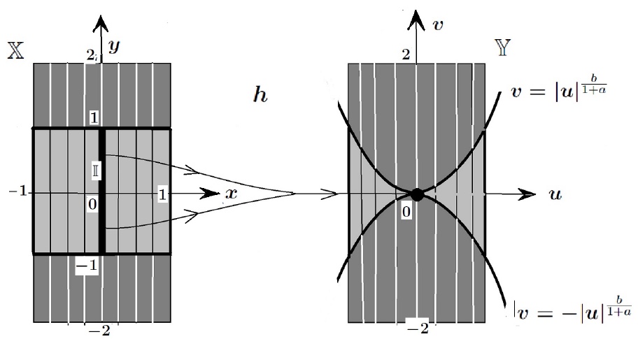
Figure 1.

∎

5.1. An extension

We just have constructed a monotone map $h\colon\overline{\mathbb{X}}\xrightarrow[]{{}_{\!\!\textnormal{onto\,\,}\!\!}}\overline{\mathbb{Y}}$ of finite energy which equals the identity on the vertical sides of the rectangle $\,\overline{\mathbb{X}}=[-1,1]\times[-2,2]\,$. However, restricted to the horizontal sides it is not the identity; it takes the form:

$$h(x,2)=(x|x|^{a},2)\;\;\;\textnormal{and}\;\;\;h(x,-2)=(x|x|^{a},-2),\;\textnormal{for}\;-1\leqslant x\leqslant 1\,.$$

We shall still need a map that is equal to the identity on the entire boundary. For this purpose we extend $\,h\,$ to a map $\,\widetilde{h}:\widetilde{\mathbb{X}}\xrightarrow[]{{}_{\!\!\textnormal{onto\,\,}\!\!}}\widetilde{\mathbb{Y}}\,$, where $\,\widetilde{\mathbb{X}}=\widetilde{\mathbb{Y}}=[-1,1]\times[-3,3]\,$, by the rule,

(5.1) $$\widetilde{h}(x,y)=\begin{cases}\Big{(}x|x|^{a}(3-y)\,+\,x(y-2)\;,\;y\Big{)},\,\,\,&\textnormal{when}\,2\leqslant y\leqslant 3\\ h(x,y)\;,\;\;&\textnormal{when}\;-2\leqslant y\leqslant 2\\ \Big{(}x|x|^{a}(3+y)\,-\,x(y+2)\;,\;y\Big{)},\,\,\,&\textnormal{when}\,-3\leqslant y\leqslant-2\,.\end{cases}$$

Clearly $\,\widetilde{h}\,$ is monotone and equal to the identity on $\,\partial\widetilde{\mathbb{X}}\,$. Just as in the computation above we see that $\,\mathsf{E}^{p}_{q}[\widetilde{h}]<\infty\,$. Proceeding further in this direction, we may extend $\,\widetilde{h}\,$ to the square $\,\mathbf{S}\stackrel{{\scriptstyle\textnormal{def}}}{{=\!\!=}}[-4,4]\times[-4,4]\,$ by letting it be equal to the identity outside $\,\widetilde{\mathbb{X}}\,$. Let us record this in the following lemma.

Lemma 5.1.

For every $\,p>2\,$ and $\,0<q<\frac{p}{p-2}$ there exists a non-injective monotone map $\,\Phi\in\mathscr{M}^{p}(\mathbf{S},\mathbf{S})$ of finite $\mathsf{E}_{q}^{p}\,$-energy, which is the identity near the boundary of $\,\mathbf{S}\,$. Precisely, we have the following average energy

(5.2) $$\mathsf{E}_{q}^{p}[\Phi]\,=\frac{1}{|\mathbf{S}|}\int_{\mathbf{S}}\left[\lvert D\Phi(y)\rvert^{p}+\frac{1}{[\,\det D\Phi(y)]^{q}}\right]\textnormal{d}y\;\;\stackrel{{\scriptstyle\textnormal{def}}}{{=\!\!=}}\mathbf{E}\,<\infty$$

where $\,|\mathbf{S}|=16\,$ is the area of the square $\mathbf{S}=[-4,4]\times[-4,4]$.

5.1.1. Rescaling

Formula (5.2) can be rescaled to an arbitrary square $\,Q\subset\mathbb{R}^{2}\,$ in place of $\,\mathbf{S}\,$. Let us discuss it in a somewhat greater context. For, choose and fix a prototype energy integral over a square $\,\mathbf{S}\subset\mathbb{R}^{2}\,$ centered at the origin and of side-length $\,L\,$,

(5.3) $$\mathscr{E}[\Phi]\stackrel{{\scriptstyle\textnormal{def}}}{{=\!\!=}}\frac{1}{|\mathbf{S}|}\int_{\mathbf{S}}\textrm{E}(D\Phi(y))\,\textnormal{d}y\;,$$

This integral is assumed to exist for some adequate mappings $\,\Phi:\mathbf{S}\xrightarrow[]{{}_{\!\!\textnormal{onto\,\,}\!\!}}\mathbf{S}\,$ , $\Phi(0)=0\,$. Note that the stored-energy integrand depends solely on the deformation gradient $\,D\Phi\,$. Now take any square $\,Q\,$ centered at $\,a\in\mathbb{R}^{2}\,$ and of side-length $\ell$. Then the mapping

(5.4) $$h_{Q}:Q\xrightarrow[]{{}_{\!\!\textnormal{onto\,\,}\!\!}}Q\;,\;\textnormal{defined by}\;\;h_{Q}(x)\stackrel{{\scriptstyle\textnormal{def}}}{{=\!\!=}}a+\frac{\ell}{L}\,\Phi\left(\frac{L}{\ell}(x-a)\right)$$

has the same average energy as $\Phi$,

(5.5) $$\mathscr{E}[h_{Q}]=\frac{1}{|\mathbf{Q}|}\int_{\mathbf{Q}}\textrm{E}(Dh_{Q}(x))\,\textnormal{d}x\;=\;\mathscr{E}[\Phi]$$

This is an obvious consequence of the chain rule $\,Dh_{Q}(x)=D\Phi(y)\,$, where $\,y=\frac{L}{\ell}(x-a)\,$ is a variable used as a substitution in the integral (5.3). For later use, it should be noted that if $\,\Phi\,$ is monotone, so is $\,h_{Q}\,$. Also, if $\,\Phi\,$ is the identity map near $\,\partial\mathbf{S}\,$ then so is $\,h_{Q}\,$ near $\,\partial Q\,$.

6. Cantor Type Construction of Example 1.9

6.1. Construction of Cantor set

We shall work with closed squares whose sides are parallel to the standard coordinate axes of $\mathbb{R}^{2}$, but most of the definitions and formulas will be coordinate-free.

6.1.1. Cornersquares

Suppose we are given a square $\,Q\subset\mathbb{R}^{2}\,$ and a parameter $\,0<\varepsilon<1\,$. Write it as $\,Q=I\times J\,$, where $\,I,J\,\subset\mathbb{R}\,$ are closed intervals of the same length $\,\ell=|I|=|J|\,$. These might be called respectively the horizontal and the vertical factors of $\,Q\,$. The notation $\,\varepsilon I\,$ and $\,\varepsilon J\,$ will stand for the intervals of the same centers but $\,\varepsilon\,$-times smaller in length, respectively. Cutting them out from $\,I\,$ and $\,J\,$ gives the decompositions:

$$I\setminus\varepsilon I=I_{-}\cup I_{+}\;\;\textnormal{and}\;\;J\setminus\varepsilon J=J^{-}\cup J^{+}\,$$

into the left and the right, as well as into the lower and the upper subintervals. Note that we suppressed the explicit dependence on $\,\varepsilon\,$ in the notation. This parameter will be determined later during our induction procedure. Now the Cartesian product consists of four sub-squares:

$$(I\setminus\varepsilon I)\times(J\setminus\varepsilon J)\;=\;Q^{+}_{+}\,\cup\,Q^{+}_{-}\,\cup\,Q^{-}_{-}\,\cup\,Q^{-}_{+}\,.$$

Explicitely, we have the formulas:

$$Q^{+}_{+}\,\stackrel{{\scriptstyle\textnormal{def}}}{{=\!\!=}}I_{+}\times J^{+}\,,\;Q^{+}_{-}\,\stackrel{{\scriptstyle\textnormal{def}}}{{=\!\!=}}I_{-}\times J^{+}\,,\,Q^{-}_{-}\,\stackrel{{\scriptstyle\textnormal{def}}}{{=\!\!=}}I_{-}\times J^{-}\,,\,Q^{-}_{+}\stackrel{{\scriptstyle\textnormal{def}}}{{=\!\!=}}I_{+}\times J^{-}\,.$$

Each of these sub-squares touches exactly one corner of $\,Q\,$, which motivates our calling $\,Q^{+}_{+}\,,\,Q^{+}_{-}\,,\,Q^{-}_{-}\,,\,Q^{-}_{+}\,\,$ the cornersquares of $\,Q\,$; more precisely, the first generation of cornersquares. We shall also spot the so-called centersquare of $\,Q\,$, defined by $\,\varepsilon Q=\varepsilon I\times\varepsilon J\,$, see the left hand side of Figure 2.

6.1.2. Second generation of cornersquares

Choose another positive $\,\varepsilon\,$-parameter, say $\,\varepsilon=\varepsilon_{2}\,$. Then every cornersquare of $\,Q\,$ gives rise to its own four cornersquares determined by this parameter, see the middle part of Figure 2. In this way we obtain sixteen cornersquares of so-called second generation. According to our notation these are:

$$Q^{++}_{++}\;\;Q^{++}_{+-}\;\;Q^{+-}_{+-}\;\;Q^{+-}_{++}\;\;$$

$$Q^{++}_{-+}\;\;Q^{++}_{--}\;\;Q^{+-}_{--}\;\;Q^{+-}_{-+}\;\;$$

$$Q^{-+}_{-+}\;\;Q^{-+}_{--}\;\;Q^{--}_{--}\;\;Q^{--}_{-+}\;\;$$

$$Q^{-+}_{++}\;\;Q^{-+}_{+-}\;\;Q^{--}_{+-}\;\;Q^{--}_{++}\;\;$$

See also the third generation of 64 cornersquares in the right hand side of Figure 2.

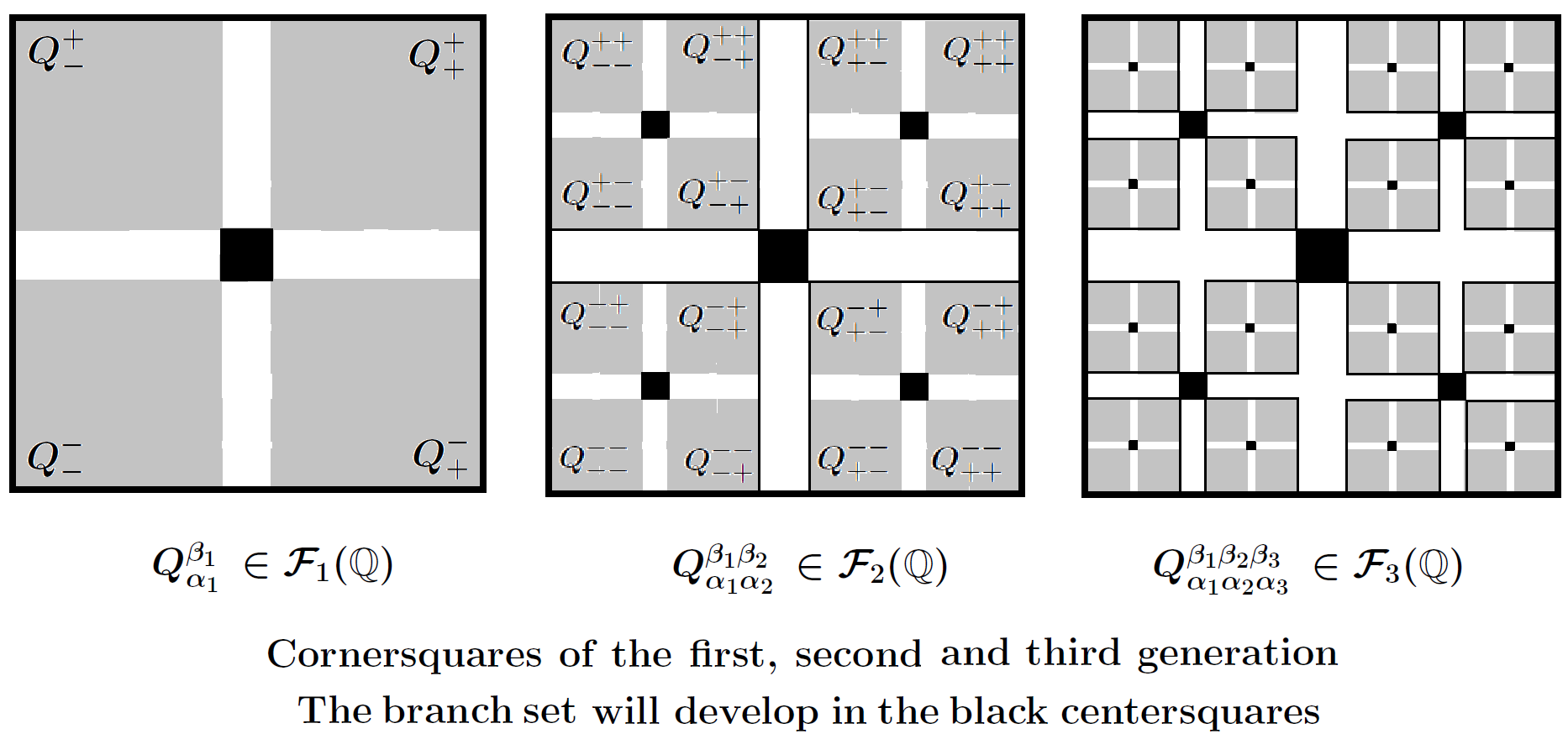
Figure 2. Cornersquares as building blocs for a Cantor type construction

6.1.3. The induction procedure

Fix a sequence of $\varepsilon\,$-parameters rapidly decreasing to 0, say $\,(\varepsilon_{1},\varepsilon_{2},...)\,$ with $\varepsilon_{n}=4^{-n}\,$. We begin with the base $\,1\times 1\,$ square $\,\mathbb{Q}\subset\mathbb{R}^{2}\,\,$ and the first $\,\varepsilon\,$- parameter equal to $\,\varepsilon_{1}\,$. This gives us the first generation of four cornersquares $\,Q^{\beta_{1}}_{\alpha_{1}}\subset\mathbb{Q}\,$, where both indices run over the set $\,\{+\,,\,-\}\,$. We let $\,\mathcal{F}_{1}\,$ denote this family of cornersquares.

In the second step we take $\varepsilon_{2}\,$ as the $\,\varepsilon\,$-parameter and look at the cornersquares of every $\,Q^{\beta_{1}}_{\alpha_{1}}\,$. Denote them by $\,Q^{\beta_{1}\,\beta_{2}}_{\alpha_{1}\,\alpha_{2}}\subset Q^{\beta_{1}}_{\alpha_{1}}\,$, where $\,\alpha_{2},\beta_{2}\in\{+\,,\,-\}\,$. They form the family $\,\mathcal{F}_{2}\,$ of second generation. More generally, given the family $\,\mathcal{F}_{n}\,$ of cornersquares $\,Q^{\beta_{1}\,\beta_{2}...\beta_{n}}_{\alpha_{1}\,\alpha_{2}...\alpha_{n}}\subset Q^{\beta_{1}\,\beta_{2}...\beta_{n-1}}_{\alpha_{1}\,\alpha_{2}...\alpha_{n-1}}\in\mathcal{F}_{n-1}\,$, we take $\,\varepsilon_{n+1}\,$ as the $\,\varepsilon\,$-parameter and adopt to the family $\,\mathcal{F}_{n+1}\,$ the $\,\varepsilon\,$-cornersquares of $\,Q^{\beta_{1}\,\beta_{2}...\beta_{n}}_{\alpha_{1}\,\alpha_{2}...\alpha_{n}}\,$; namely,

$$\,Q^{\beta_{1}\,\beta_{2}...\beta_{n}+}_{\alpha_{1}\,\alpha_{2}...\alpha_{n}+}\;,\;Q^{\beta_{1}\,\beta_{2}...\beta_{n}+}_{\alpha_{1}\,\alpha_{2}...\alpha_{n}-}\;,\;Q^{\beta_{1}\,\beta_{2}...\beta_{n}-}_{\alpha_{1}\,\alpha_{2}...\alpha_{n}-}\;,\;\,Q^{\beta_{1}\,\beta_{2}...\beta_{n}-}_{\alpha_{1}\,\alpha_{2}...\alpha_{n}+}\;\in\;\mathcal{F}_{n+1}\,.$$

Thus $\,\mathcal{F}_{n+1}\,$ consists of $\,4^{n+1}\,$ cornersquares denoted by $\,Q^{\beta_{1}\,\beta_{2}...\beta_{n}\beta{n+1}}_{\alpha_{1}\,\alpha_{2}...\alpha_{n}\alpha_{n+1}}\,.$ This process continuous indefinitely.

6.1.4. The size of squares in $\,\mathcal{F}_{n}\,$ and their total area

Let us compare the side-length of squares in $\,\mathcal{F}_{n+1}\,$ with those in $\,\mathcal{F}_{n}\,$. Every member of $\,\mathcal{F}_{n+1}\,$ is a cornersquare of a $\,Q\in\mathcal{F}_{n}\,$ via the parameter $\,\varepsilon=\varepsilon_{n+1}\,$. Let $\,\ell\,$ denote the sidelength of $\,Q\,$. We remove from $\,Q\,$ its centersquare $\,\varepsilon Q\,$. Thus each of the remaining four cornersquares has side-length $\,\frac{1}{2}(1-\epsilon)\ell\,$. For $\,n=1\,$ this equals $\,\frac{1}{2}(1-\epsilon_{1})\,$. Hence, by induction, the side-length of squares in $\,\mathcal{F}_{n}\,$ equals $\,\frac{1}{2^{n}}(1-\varepsilon_{1})(1-\varepsilon_{2})\cdots(1-\varepsilon_{n})\,<\frac{1}{2^{n}}\,$. We have $\,4^{n}\,$ such squares. This sums up to the total area of the union

$$\left|\,\bigcup\mathcal{F}_{n}\,\right|=(1-\varepsilon_{1})^{2}(1-\varepsilon_{2})^{2}\cdots(1-\varepsilon_{n})^{2}$$

6.1.5. The Cantor set

We have a decreasing sequence of compact sets $\,\bigcup\mathcal{F}_{1}\supsetneq\bigcup\mathcal{F}_{2}\supsetneq...\supsetneq\bigcup\mathcal{F}_{n}...\,$. Cantor’s Theorem tells us that their intersection is not empty,

$$\mathcal{C}\stackrel{{\scriptstyle\textnormal{def}}}{{=\!\!=}}\bigcap_{n-1}^{\infty}\left(\bigcup\mathcal{F}_{n}\right)\;\not=\emptyset$$

The measure of this Cantor set is positive.

(6.1) $$\left|\,\mathcal{C}\,\right|\;=\;\lim_{n\rightarrow\infty}\left|\,\bigcup\mathcal{F}_{n}\,\right|=\prod_{k=1}^{\infty}(1-\varepsilon_{k})^{2}\,>0$$

The latter inequality is a consequence of $\,\sum_{k=1}^{\infty}\,\varepsilon_{k}\,<\infty\,$. Every point in $\,\mathcal{C}\,$ is obtained as intersection of exactly one decreasing sequence of the form

$$\,Q^{\beta_{1}}_{\alpha_{1}}\supsetneq Q^{\beta_{1}\beta_{2}}_{\alpha_{1}\alpha_{2}}\supsetneq\;...\;\supsetneq Q^{\beta_{1}\beta_{2}...\beta_{n}}_{\alpha_{1}\alpha_{2}...\alpha_{n}}\;...\,$$

An obvious consequence of this is:

Lemma 6.1.

Every open set that intersects $\,\mathcal{C}\,$ contains a square, say $\,Q\in\mathcal{F}_{n}$ for sufficiently large $\,n\,$ which, in turn, contains its centersquare $\,\varepsilon_{n}Q\subset Q\,$.

The idea behind this lemma is a monotone mapping $\,h:\mathbb{Q}\xrightarrow[]{{}_{\!\!\textnormal{onto\,\,}\!\!}}\mathbb{Q}\,$ whose branch set will materialize in the centersquares.

6.2. A monotone map $\,h:\mathbb{Q}\xrightarrow[]{{}_{\!\!\textnormal{onto\,\,}\!\!}}\mathbb{Q}\,$

We let $\,\mathscr{G}\,$ denote the family of centersquares of all generations. From now on the need will not arise for the explicit dependence on multi-indices in the notation of centersquares. For every $\,Q\in\mathscr{G}\,$ we have a monotone map $\,h_{Q}:Q\xrightarrow[]{{}_{\!\!\textnormal{onto\,\,}\!\!}}Q\,$ defined by Formula (5.4) with $\,\Phi\,$ given in Lemma 5.1. Thus the average $\,\textsf{E}^{p}_{q}\,$-energy of $\,h_{Q}\,$ does not depend on $\,Q\,$ and equals $\,\mathbf{E}\,$. In particular,

(6.2) $$\int_{Q}\lvert Dh_{Q}(x)\rvert^{p}\,\textnormal{d}x\;<\int_{Q}\Big{(}\lvert Dh_{Q}(x)\rvert^{p}\,+[J_{h_{Q}}(x)]^{-q}\;\Big{)}\textnormal{d}x\;=|Q|\,\mathbf{E}\,.$$

Recall that $\,h_{Q}\,$ equals the identity map near $\,\partial Q\,$. Now we can define the map $\,h\in\mathscr{M}^{p}(\overline{\mathbb{Q}},\overline{\mathbb{Q}})\,$ that is hunted by Example  1.9.

Definition 6.2.

We define the map $\,h:\mathbb{Q}\xrightarrow[]{{}_{\!\!\textnormal{onto\,\,}\!\!}}\mathbb{Q}\,$ by setting:

(6.3) $$h(x)=\begin{cases}h_{Q}(x),\,\,\,&\textnormal{whenever }\,x\in Q\in\mathscr{G}\\ x\,,\,&\textnormal{otherwise.}\end{cases}$$

Let us subtract the identity map.

(6.4) $$h(x)-x=\begin{cases}h_{Q}(x)-x\,\stackrel{{\scriptstyle\textnormal{def}}}{{=\!\!=}}f_{Q}(x),\,\,\,&\textnormal{whenever }\,x\in Q\in\mathscr{G}\\ 0\,,\,&\textnormal{otherwise.}\end{cases}$$

One advantage of using this is that $\,f_{Q}\in\mathscr{W}^{1,p}_{0}(Q)\,$. Actually, $\,f_{Q}\,$ vanishes near $\,\partial Q\,$. We have the infinite series

$$\,h(x)-x=\sum_{\mathbb{Q}\in\mathscr{G}}f_{Q}(x)\,,\quad\textnormal{in which}\quad\sum_{\mathbb{Q}\in\mathscr{G}}\int_{Q}|Df_{Q}|^{p}\;<\infty\,.$$

This latter inequality is due to the estimate (6.2). Now comes a general fact (rather folklore) about Sobolev functions:

Lemma 6.3.

Let $\,\Omega\subset\mathbb{R}^{n}\,$ be a bounded domain and $\,\Omega_{i}\subset\Omega\,,i=1,2,...\,$ disjoint open subsets. Suppose we are given functions $\,f_{i}\in\mathscr{W}^{1,p}_{0}(\Omega_{i})\,$ such that $\,\sum_{i=1}^{\infty}\int_{\Omega_{i}}|Df_{i}(x)|^{p}\,\textnormal{d}x\,<\infty\,$. Then the function

$$f(x)=\begin{cases}f_{i}(x),\,\,\,&\textnormal{whenever }\,x\in\Omega_{i}\\ 0\,,\,&\textnormal{otherwise}\end{cases}$$

lies in the space $\,\mathscr{W}^{1,p}_{0}(\Omega)\,$.

We conclude that $\,h\in\mathscr{W}^{1,p}(\mathbb{Q},\mathbb{Q})\,$ with $\,p>2\,$ and, as such, is continuous on $\,\overline{\mathbb{Q}}\,$. As regards monotonicity, for each square (continuum) $\,Q\,\in\mathscr{G}\,$ the mapping $\,h:Q\xrightarrow[]{{}_{\!\!\textnormal{onto\,\,}\!\!}}Q\,$ is monotone and $\,h\,$ is the identity outside those continua. This is enough to conclude that $\,h:\overline{\mathbb{Q}}\xrightarrow[]{{}_{\!\!\textnormal{onto\,\,}\!\!}}\overline{\mathbb{Q}}\,$ is monotone. We leave the details to the reader.

Finally, every point of the Cantor set $\,\mathcal{C}\,$ belongs to the branch set of $\,h\,$. Indeed, by Lemma 6.1, any neighborhood of this point contains a square $\,Q\in\mathscr{G}\,$ in which $\,h=h_{Q}\,$ fails to be injective. Thus the branch set $\,\mathcal{B}_{h}\,$ contains the Cantor set $\,\mathcal{C}\,$ and, therefore, has positive measure. On the other hand, by the very definition, $\,h(x)\equiv x\,$ on $\mathcal{C}\,$. Therefore $\,h(\mathcal{B}_{h})\,$ also contains $\,\mathcal{C}\,$, so $\,h(\mathcal{B}_{h})\,$ has positive measure as well.

Remark 6.4.

The branch set $\,\mathcal{B}_{h}\,$ consists precisely of the Cantor set $\,\mathcal{C}\,$ and vertical segments in the centersquares $\,Q\in\mathscr{G}\,$, which are squeezed to the centers. This makes it clear that $\,h(\mathcal{B}_{h})\,=\mathcal{C}\,$. It should be noted that the branch set $\mathcal{B}_{h}$ can have nearly full measure. This follows from the formula (6.1) by letting $\varepsilon_{k}>0$ arbitrarily small.

The proof of Example 1.9 is complete.

6.3. Greater generality

We are now in a position to appreciate more general approach to the construction presented above. Let us begin with an arbitrary bounded discrete set $\,\mathbf{G}\,$ of points in $\,\mathbb{R}^{2}\,$ whose limit set, denoted by $\,\mathbf{C}\,$, has positive area, see Figure 3. Clearly, $\,\mathbf{G}\,$ is necessarily countable. Moreover, $\,\mathbf{C}\cup\mathbf{G}\,$ is a compact subset of a bounded domain $\,\Omega\subset\mathbb{R}^{2}\,$. Given a point in $\,\mathbf{G}\,$ we may (and do) choose a square $\,Q\subset\Omega\setminus\mathbf{C}\,$ centered at this point and small enough so that the family of all such squares, denoted as before by $\,\mathscr{G}$, is disjoint. Analogously to Lemma 6.1, every open set that intersects $\,\mathbf{C}\,$ contains a square in $\mathscr{G}\,$.

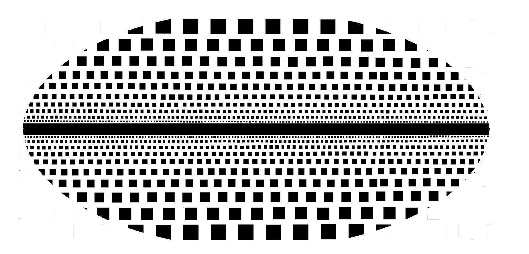
Figure 3. Squares approaching the limit set

To every $\,Q\in\mathscr{G}\,$ there corresponds a monotone map $\,h_{Q}:Q\xrightarrow[]{{}_{\!\!\textnormal{onto\,\,}\!\!}}Q\,$ equal to the identity near $\,\partial Q\,$. Recall the inequality (6.2),

(6.5) $$\int_{Q}|Dh_{Q}(x)^{p}\,\textnormal{d}x\;<\int_{Q}\Big{(}|Dh_{Q}(x)^{p}\,+[J_{h_{Q}}(x)]^{-q}\;\Big{)}\textnormal{d}x\;=|Q|\,\mathbf{E}\,.$$

This yields

$$\sum_{Q\in\mathscr{G}}\int_{Q}|Dh_{Q}(x)^{p}\,\textnormal{d}x<\sum_{Q\in\mathscr{G}}\textsf{E}^{p}_{q}[h_{Q}]\;=\mathbf{E}\sum_{Q\in\mathscr{G}}|Q|\,<\mathbf{L}|\Omega|<\infty\,.$$

It is precisely this property that one needs to infer $\,g\in\mathscr{W}^{1,p}(\Omega)\cap\mathscr{C}(\overline{\Omega})\,.$ Exactly the same way as in Formula (6.3), we define a map $\,g:\Omega\xrightarrow[]{{}_{\!\!\textnormal{onto\,\,}\!\!}}\Omega\,$ by the rule,

(6.6) $$g(x)=\begin{cases}h_{Q}(x),\,\,\,&\textnormal{whenever }\,x\in Q\in\mathscr{G}\\ x\,,\,&\textnormal{otherwise.}\end{cases}$$

Then we conclude in much the same way that $\,g\in\mathscr{M}^{p}(\overline{\Omega},\overline{\Omega})\,$, $\,\textsf{E}^{p}_{q}[g]\,<\infty\,$, $\,|\mathcal{B}_{g}|>0\,$ and $\,|g(\mathcal{B}_{g})|>0\,$.

7. Proof of Theorem 1.2

Let $\mathbb{X}$ and $\mathbb{Y}$ be $\ell$-connected bounded Lipschitz domains in $\mathbb{R}^{2}$. Consider a family $\mathcal{F}$ of Sobolev orientation-preserving monotone mappings $h\colon\overline{\mathbb{X}}\xrightarrow[]{{}_{\!\!\textnormal{onto\,\,}\!\!}}\overline{\mathbb{Y}}$ such that

(7.1) $$\mathsf{E}^{p}_{q}[h]=\int_{\mathbb{X}}\left(\lvert Dh\rvert^{p}+\frac{1}{J_{h}^{q}}\right)\leqslant E$$

for all $h\in\mathcal{F}$. Here $\mathbb{X},\mathbb{Y}$, $p\geqslant 2$, $q>0$ and $E<\infty$ are fixed.

Lemma 7.1.

The family $\mathcal{F}$ is equicontinuous. Precisely, there is a constant $C$ such that

(7.2) $$\lvert h(x_{1})-h(x_{2})\rvert^{2}\leqslant\frac{C\cdot E}{\log\left(1+\frac{C}{\lvert x_{1}-x_{2}\rvert}\right)}$$

for all $h\in\mathcal{F}$ and distinct points $x_{1},x_{2}\in\overline{\mathbb{X}}$.

Proof.

Since $J_{h}\geqslant 0$ almost everywhere in $\mathbb{X}$ we have $h\in\mathscr{M}^{p}(\overline{\mathbb{X}},\overline{\mathbb{Y}})$. Now, for proving (7.2) we may assume (equivalently) that $h\in\mathscr{H}^{p}(\mathbb{X},\mathbb{Y})$ with $\mathsf{E}^{p}_{q}[h]<\infty$, thanks to Theorem 1.1. If $\mathbb{X}$ is multiple connected $\ell\geqslant 2$, then the modulus of continuity estimate (7.2) simply follows from the fact that the Dirichlet energy of $h$ is uniformly bounded by the value of Neohookean energy $E$, see Lemma 2.2. Therefore, it suffices to consider the case of simply connected domains and $p=2$. It is worth recalling that if $\ell=1$, then $\int_{\mathbb{X}}\lvert Dh\rvert^{2}\leqslant E$ is not enough to imply (7.2), see Remark 2.3.

Let $\ell=1$ and $p=2$. We may assume without loss of generality that $\mathbb{X}=\mathbb{D}=\mathbb{Y}$. Indeed, for any bounded Lipschitz domain $\mathbb{Y}$ there exists a global bi-Lipschitz change of variables $\Phi\colon\mathbb{C}\to\mathbb{C}$ for which $\Phi(\mathbb{Y})$ is the unit disk. Since the finiteness of the $\mathsf{E}^{2}_{q}$-energy is preserved under a bi-Lipschitz change of variables in both the target $\mathbb{Y}$ and the domain $\mathbb{X}$, we assume that $\mathbb{X}$ and $\mathbb{Y}$ are unit disks. Choose and fix any disk $B=B(x_{\circ},\delta)\Subset\mathbb{X}$. We have, for every $h\in\mathcal{F}$

$$\begin{split}\lvert B\rvert&=\int_{B}J_{h}^{\frac{q}{q+1}}\cdot\frac{1}{J_{h}^{\frac{q}{q+1}}}\\ &\leqslant\left(\int_{B}J_{h}\right)^{\frac{q}{q+1}}\left(\int_{B}\frac{1}{J^{q}_{h}}\right)^{\frac{1}{q+1}}\leqslant\lvert h(B)\rvert^{\frac{q}{q+1}}\cdot E^{\frac{1}{q+1}}\,.\end{split}$$

Hence

$$\lvert h(B)\rvert\geqslant\lvert B\rvert^{\frac{q+1}{q}}E^{-\frac{1}{q}}\quad\textnormal{constant independent of }h\in\mathcal{F}\,.$$

Choose and fix $\varepsilon>0$ such that the annulus

$$\Delta_{\varepsilon}=\{y\in\mathbb{Y}\colon\operatorname{dist}(y,\partial\mathbb{Y})\leqslant\varepsilon\}$$

has measure smaller than $\lvert B\rvert^{\frac{q+1}{q}}E^{-\frac{1}{q}}$. Thus $h(B)\not\subset\Delta_{\varepsilon}$ and, therefore, there is a point $a\in B\Subset\mathbb{X}$ such that $\lvert h(a)\rvert<1-\varepsilon$. In other words for every $h\in\mathcal{F}$ we can find a point $a\in\mathbb{X}$, with $\lvert a\rvert\leqslant 1-\delta$, and $b=h(a)\in\mathbb{Y}$, with $\lvert b\rvert<1-\varepsilon$. Now consider conformal mappings $\varphi\colon\overline{\mathbb{X}}\xrightarrow[]{{}_{\!\!\textnormal{onto\,\,}\!\!}}\overline{\mathbb{X}}$, $\varphi(a)=0$, and $\psi\colon\overline{\mathbb{Y}}\to\overline{\mathbb{Y}}$, $\psi(b)=0$. Both mappings are bi-Lipschitz with bi-Lipschitz constants independent of $a$ and $b$. Thus the energy $\psi\circ h\circ\varphi\colon\mathbb{X}\xrightarrow[]{{}_{\!\!\textnormal{onto\,\,}\!\!}}\mathbb{Y}$ is controlled from above by that of $h$ uniformly in $\mathcal{F}$. Therefore, we may (and do) assume that $h(0)=0$. This leads us to the case of a homeomorphism $h\colon\mathbb{D}\setminus\{0\}\xrightarrow[]{{}_{\!\!\textnormal{onto\,\,}\!\!}}\mathbb{D}\setminus\{0\}$; that is, between doubly connected domains. Finally, the inequality (7.2) follows from Lemma 2.2, completing the proof of Lemma 7.1. ∎

Proof of Theorem 1.2.

We apply the direct method in the calculus of variations. For that we take a minimizing sequence $h_{k}\in\mathscr{M}^{p}(\overline{\mathbb{X}},\overline{\mathbb{Y}})$ of the neohookean energy $\mathsf{E}_{q}^{p}$ which converges weakly to $h_{\circ}$ in $\mathscr{W}^{1,p}(\mathbb{X},\mathbb{C})$. Note that here we also used our standing assumption that the class of admissible homeomorphisms is nonempty. Therefore, by Lemma 2.7 we have

(7.3) $$\mathsf{E}^{p}_{q}[h_{\circ}]\leqslant\liminf_{k\to\infty}\mathsf{E}^{p}_{q}[h_{k}]=\underset{h\in\mathscr{M}^{p}(\overline{\mathbb{X}},\overline{\mathbb{Y}})}{\inf}\mathsf{E}_{q}^{p}[h]\,.$$

Since $\mathsf{E}_{q}^{p}[h_{k}]\leqslant E<\infty$ for every $k\in\mathbb{N}$ and $h_{k}\to h_{\circ}$ weakly in $\mathscr{W}^{1,p}(\mathbb{X},\mathbb{C})$ applying Lemma 7.1 we see that the sequence $h_{k}$ also converges uniformly to $h_{\circ}$ in $\overline{\mathbb{X}}$. Now the mapping $h_{\circ}$, being a uniform limit of monotone mappings $h_{k}\colon\overline{\mathbb{X}}\xrightarrow[]{{}_{\!\!\textnormal{onto\,\,}\!\!}}\overline{\mathbb{Y}}$, is a monotone map from $\overline{\mathbb{X}}$ onto $\overline{\mathbb{Y}}$. Therefore, $h_{\circ}\in\mathscr{M}^{p}(\overline{\mathbb{X}},\overline{\mathbb{Y}})$. Combining this with (7.3) we have

$$\mathsf{E}^{p}_{q}[h_{\circ}]\leqslant\underset{h\in\mathscr{M}^{p}(\overline{\mathbb{X}},\overline{\mathbb{Y}})}{\inf}\mathsf{E}_{q}^{p}[h]\leqslant\mathsf{E}^{p}_{q}[h_{\circ}]\,,$$

finishing the proof of Theorem 1.2. ∎

8. Proof of Theorem 1.5

Proof.

First we are going to estimate the distortion function

$$1\,\leqslant\,\mathscr{K}_{h}(x)\,\stackrel{{\scriptstyle\textnormal{def}}}{{=\!\!=}}\,\frac{|Dh(x)|^{2}}{2J_{h}(x)}$$

by using Young’s inequality:

$$ABC\,\leqslant\,\alpha A^{\frac{1}{\alpha}}+\beta B^{\frac{1}{\beta}}+\gamma C^{\frac{1}{\gamma}},\,\,\,\,A,B,C\geqslant 0;\,\alpha,\beta,\gamma\geqslant 0,\,\alpha+\beta+\gamma=1$$

where we add here to the convention that $\gamma C^{\frac{1}{\gamma}}=0$ for $\gamma=0$. The pointwise estimate of $\mathscr{K}_{h}$ by means of the energy integrand reads as when $p>2$.

$$2\mathscr{K}_{h}(x)\, \leqslant \,\frac{2}{p}|Dh|^{p}+\frac{1}{q}\frac{1}{J_{h}^{q}}+\left(1-\frac{2}{p}-\frac{1}{q}\right)\cdot 1$$

$$\leqslant \frac{2}{p}|Dh|^{p}+\frac{1}{q}\frac{1}{J_{h}^{q}}+\left(1-\frac{2}{p}-\frac{1}{q}\right)\mathscr{K}_{h}$$

Hence

$$\mathscr{K}_{h}\,\leqslant\,|Dh|^{p}+\frac{1}{J_{h}^{q}}=\mathsf{E}(|Dh|,\det Dh)$$

Integrating over $\Omega$ we obtain

$$\|\mathscr{K}_{h}\|_{\mathscr{L}^{1}(\Omega)}\,=\,\int_{\Omega}\mathscr{K}_{h}(x)\textnormal{d}x\,<\infty$$

For Remark 1.6 concerning the case $p=2$ and $q=\infty$ we argue as follows.

$$\mathscr{K}_{h}\,\,=\,\,\frac{|Dh|^{2}}{2J_{h}}\,\,\leqslant\,\,\frac{C}{2}|Dh|^{2}$$

Hence

$$\int_{\mathbb{X}}\mathscr{K}_{h}\,\,<\,\,\frac{C}{2}\int_{\mathbb{X}}|Dh|^{2}\,\,<\,\,\infty$$

In either case, $p>2$ or $p=2$ we see that the map $h\in\mathscr{W}^{1,2}(\Omega,\mathbb{R}^{2})$ has integrable distortion. It is known [26] that such mappings $h\colon\Omega\rightarrow\mathbb{R}^{2}$ are discrete and open. In particular $h(\Omega)$, being an open subset of $\overline{\mathbb{Y}}$, is contained in $\mathbb{Y}$. Next we show that $h\colon\Omega\xrightarrow[]{{}_{\!\!\textnormal{onto\,\,}\!\!}}h(\Omega)$ is injective. To this effect suppose, to the contrary, that $h(x_{1})=h(x_{2})\stackrel{{\scriptstyle\textnormal{def}}}{{=\!\!=}}y_{\circ}\in h(\Omega)$ for some points $x_{1}\neq x_{2}$ in $\Omega$. The preimage $h^{-1}(y_{\circ})$ under the map $h\colon\overline{\mathbb{X}}\xrightarrow[]{{}_{\!\!\textnormal{onto\,\,}\!\!}}\overline{\mathbb{Y}}$ is a continuum in $\overline{\mathbb{X}}$ which contains $x_{1}$, $x_{2}\in\Omega$. This contradicts discreteness of $h\colon\Omega\rightarrow\mathbb{R}^{2}$.

Since $\Omega\Subset\mathbb{X}$ is arbitrary it follows that $h\colon\mathbb{X}\xrightarrow[]{{}_{\!\!\textnormal{onto\,\,}\!\!}}h(\mathbb{X})$ is a homeomorphism as well. Finally, it remains to show that $h(\mathbb{X})=\mathbb{Y}$. Certainly, $h(\mathbb{X})$ being an open subset of $\overline{\mathbb{Y}}$, is contained in $\mathbb{Y}$.

Suppose there is $y_{\circ}\in\mathbb{Y}\setminus h(\mathbb{X})$. But $y_{\circ}\in{\overline{\mathbb{Y}}}=h(\overline{\mathbb{X}})$, so $y_{\circ}=h(x_{\circ})$ for some $x_{\circ}\in\overline{\mathbb{X}}$. On the other hand, the map $h\colon\overline{\mathbb{X}}\xrightarrow[]{{}_{\!\!\textnormal{onto\,\,}\!\!}}\overline{\mathbb{Y}}$, being monotone, takes $\partial\mathbb{X}$ onto $\partial\mathbb{Y}$.

$$h(\partial\mathbb{X})\,=\,\partial\mathbb{Y}$$

This means that $x_{\circ}\notin\partial\mathbb{X}$, because $h(x_{\circ})=y_{\circ}\notin\partial\mathbb{Y}$.
In conclusion,

$$h(\mathbb{X})=\mathbb{Y}.$$

∎

9. Proof of Theorem 1.10

Proof.

First note that $s>p$ and $|Dh|^{s}\in\mathscr{L}_{\operatorname{loc}}^{1}(\mathbb{X})$. The idea of the proof is to infer from  (1.7) that

(9.1) $$\frac{1}{J_{h}}\in\mathscr{L}_{\operatorname{loc}}^{\frac{sq}{p}}(\mathbb{X})\,.$$

For this purpose consider the functions

(9.2) $$\Phi=\left(1-\frac{p}{2}\right)|Dh|^{p}+\frac{1+q}{J_{h}^{q}}\in\mathscr{L}_{\operatorname{loc}}^{1}(\mathbb{X})$$

(9.3) $$\Psi=2p|Dh|^{p-2}\overline{h_{z}}h_{\overline{z}}\in\mathscr{L}_{\operatorname{loc}}^{r}(\mathbb{X},\mathbb{C}),\,\,\,\textnormal{ where }r=\frac{s}{p}>1$$

The equation  (1.7) reads as

(9.4) $$\Phi_{\overline{z}}=\Psi_{z},\,\,\,\textnormal{ in the sense of distributions }$$

We first observe that:

Lemma 9.1.

For every subdomain $\Omega\Subset\mathbb{X}$ compactly contained in $\mathbb{X}$ it holds that

$$\Phi\in\mathscr{L}^{r}(\Omega)$$

Proof.

of Lemma 9.1. Choose and fix a function $\lambda\in C_{0}^{\infty}(\mathbb{X})$ which equals $1$ in a neighborhood of $\overline{\Omega}\subset\mathbb{X}$. Then consider the expression defined in the entire complex plane by the rule

(9.5) $$\lambda\Phi-S\lambda\Psi$$

where $S\colon\mathscr{L}^{r}(\mathbb{C})\rightarrow\mathscr{L}^{r}(\mathbb{C})$, is the Beurling-Ahlfors transform.

$$(Sf)(z)=-\frac{1}{\pi}\int_{\mathbb{C}}\int\frac{f(\xi)\textnormal{d}\xi}{(z-\xi)^{2}},\,\,\,\textnormal{ for }f\in\mathscr{L}^{r}(\mathbb{C})$$

The following identity is characteristic of Beurling-Ahlfors transform

$$\frac{\partial}{\partial\overline{z}}(Sf)=\frac{\partial}{\partial z}f\,\,\textnormal{ for }f\in\mathscr{L}^{r}(\mathbb{C})$$

The complex derivatives are understood in the sense of distributions. We may, and do, apply this identity to $f=\lambda\Psi$. Differentiating the expression (9.5) with respect to $\overline{z}$ yields

$$\frac{\partial}{\partial\overline{z}}\left[\lambda\Phi-S\lambda\Psi\right] = \frac{\partial}{\partial\overline{z}}\left[\lambda\Phi\right]-\frac{\partial}{\partial z}\left[\lambda\Psi\right]$$

$$= \lambda_{\overline{z}}\Phi+\lambda\Phi_{\overline{z}}-\lambda_{z}\Psi-\lambda\Psi_{z}$$

$$= \lambda_{\overline{z}}\Phi-\lambda_{z}\Psi=0\textnormal{ in a neighborhood of }\overline{\Omega}.$$

Here we used the equation (9.4) and the fact the $\lambda\equiv 1$ in a neighborhood of $\overline{\Omega}$. Thus, by Weyl’s Lemma the function:

$$H=\lambda\Phi-S\lambda\Psi$$

is holomorphic in a neighborhood of $\overline{\Omega}\subset\mathbb{X}$ so $H\in\mathscr{L}^{r}(\Omega)$. In this neighborhood we express $H$ as

$$H(z)=\Phi(z)+\frac{1}{\pi}\int_{\mathbb{C}}\int\frac{\lambda(\xi)\Psi(\xi)\textnormal{d}\xi}{(z-\xi)^{2}}$$

The latter integral, being the Beurling-Ahlfors transform of $\lambda\Psi\in\mathscr{L}^{r}(\mathbb{C})$, represents a function in $\mathscr{L}^{r}(\mathbb{C})$. In conclusion $\Phi\in\mathscr{L}^{r}(\Omega)$. ∎

Now it follows by (9.2) that $J_{h}^{-q}\in\mathscr{L}^{r}_{\operatorname{loc}}(\Omega)$, as claimed in (9.1). Combining this with the assumption $|Dh|^{s}\in\mathscr{L}_{\operatorname{loc}}^{1}(\mathbb{X})$ we have

$$\int_{\Omega}\left(|Dh|^{s}+{J_{h}^{-\frac{sq}{p}}}\right)<\infty\,,$$

where $\Omega\Subset\mathbb{X}$, $s>2$ and $\frac{sq}{p}\geqslant\frac{s}{s-2}$. We are now in a position to apply Theorem 1.5 for $s$ in place of $p$ and $\frac{sq}{p}$ in place of $q$. Therefore,

$$h\colon\mathbb{X}\xrightarrow[]{{}_{\!\!\textnormal{onto\,\,}\!\!}}\mathbb{Y}$$

is a homeomorphism. ∎

References

• [1] S. S. Antman, Nonlinear problems of elasticity. Applied Mathematical Sciences, 107. Springer-Verlag, New York, 1995.
• [2] K. Astala, T. Iwaniec, and G. Martin, Deformations of annuli with smallest mean distortion, Arch. Ration. Mech. Anal. 195 (2010), no. 3, 899–921.
• [3] K. Astala, T. Iwaniec, and G. Martin, Elliptic partial differential equations and quasiconformal mappings in the plane, Princeton University Press, 2009.
• [4] J. M. Ball, Convexity conditions and existence theorems in nonlinear elasticity, Arch. Rational Mech. Anal. 63 (1976/77), no. 4, 337–403.
• [5] J. M. Ball, Global invertibility of Sobolev functions and the interpenetration of matter, Proc. Roy. Soc. Edinburgh Sect. A, 88 (1981), 315–328.
• [6] J. M. Ball, Existence of solutions in finite elasticity, Proceedings of the IUTAM Symposium on Finite Elasticity. Martinus Nijhoff, 1981.
• [7] J. M. Ball, Discontinuous equilibrium solutions and cavitation in nonlinear elasticity, Philos. Trans. R. Soc. Lond. A 306 (1982) 557–611.
• [8] P. Bauman, D. Phillips, and N. Owen, Maximum principles and a priori estimates for an incompressible material in nonlinear elasticity, Comm. Partial Differential Equations 17 (1992), no. 7-8, 1185–1212.
• [9] P. G. Ciarlet, Mathematical elasticity Vol. I. Three-dimensional elasticity, Studies in Mathematics and its Applications, 20. North-Holland Publishing Co., Amsterdam, 1988.
• [10] P. G. Ciarlet and J. Nečas, Injectivity and self-contact in nonlinear elasticity, Arch. Rational Mech. Anal. 97 (1987), no. 3, 171–188.
• [11] S. Conti and C. De Lellis, Some remarks on the theory of elasticity for compressible Neohookean materials, Ann. Sc. Norm. Super. Pisa Cl. Sci. (5) 2 (2003) 521–549.
• [12] J. Cristina, T. Iwaniec, L. V. Kovalev, and J. Onninen, The Hopf-Laplace equation: harmonicity and regularity, Ann. Sc. Norm. Super. Pisa Cl. Sci. (5) 13 (2014), no. 4, 1145–1187.
• [13] L. C. Evans, Quasiconvexity and partial regularity in the calculus of variations, Arch. Rational Mech. Anal. 95 (1986), no. 3, 227–252.
• [14] I. Fonseca and W. Gangbo, Local invertibility of Sobolev functions, SIAM J. Math. Anal. 26 (1995), no. 2, 280–304.
• [15] P. Hajłasz, J. Malý, Approximation in Sobolev spaces of nonlinear expressions involving the gradient, Ark. Mat. 40 (2002), no. 2, 245–274.
• [16] S. Hencl and P. Koskela Lectures on mappings of finite distortion, Lecture Notes in Mathematics 2096, Springer, (2014).
• [17] T. Iwaniec and G. Martin, Geometric Function Theory and Non-linear Analysis, Oxford Mathematical Monographs, Oxford University Press, 2001.
• [18] T. Iwaniec, P. Koskela, and J. Onninen, Mappings of finite distortion: monotonicity and continuity, Invent. Math. 144 (2001), no. 3, 507-?531.
• [19] T. Iwaniec, L. V. Kovalev, and J. Onninen, Lipschitz regularity for inner-variational equations, Duke Math. J. 162 (2013), no. 4, 643–672.
• [20] T. Iwaniec and J. Onninen, Neohookean deformations of annuli, existence, uniqueness and radial symmetry, Math. Ann. 348 (2010), no. 1, 35–55.
• [21] T. Iwaniec and J. Onninen, Deformations of finite conformal energy: Boundary behavior and limit theorems, Trans. Amer. Math. Soc. 363 (2011), no. 11, 5605–5648.
• [22] T. Iwaniec and J. Onninen, $n$-Harmonic mappings between annuli Mem. Amer. Math. Soc. 218 (2012).
• [23] T. Iwaniec and J. Onninen, Mappings of least Dirichlet energy and their Hopf differentials, Arch. Ration. Mech. Anal. 209 (2013), no. 2, 401–453.
• [24] T. Iwaniec and J. Onninen, Monotone Sobolev mappings of planar domains and surfaces, Arch. Ration. Mech. Anal. 219 (2016), no. 1, 159–181.
• [25] T. Iwaniec and J. Onninen, Limits of Sobolev homeomorphisms, J. Eur. Math. Soc. (JEMS) 19 (2017), no. 2, 473-505.
• [26] T. Iwaniec and V. Šverák, On mappings with integrable dilatation, Proc. Amer. Math. Soc. 118 (1993), no. 1, 181–188.
• [27] A. Koski and J. Onninen, Radial symmetry of p-harmonic minimizers, Arch. Ration. Mech. Anal. 230 (2018), no. 1, 321–342.
• [28] H. Lebesgue, Sur le probléme de Dirichlet, Rend. Circ. Palermo 27 (1907), 371–402.
• [29] C. B. Morrey, The Topology of (Path) Surfaces, Amer. J. Math. 57 (1935), no. 1, 17–50.
• [30] C. B. Morrey., Quasiconvexity and the semicontinuity of multiple integrals, Pacific J. Math. 2 (1952) 25–53.
• [31] Yu. G. Reshetnyak, Space mappings with bounded distortion, American Mathematical Society, Providence, RI, 1989.
• [32] J. Sivaloganathan and S. J. Spector, Necessary conditions for a minimum at a radial cavitating singularity in nonlinear elasticity, Ann. Inst. H. Poincaré Anal. Non Linéaire 25 (2008), no. 1, 201–213.