Optomagnonic Barnett effect

Abstract

Combining the technologies of quantum optics and magnonics, we find that the circularly polarized laser can dynamically realize the quasiequilibrium magnon Bose-Einstein condensates (BEC). The Zeeman coupling between the laser and spins generates the optical Barnett field, and its direction is controllable by switching the laser chirality. We show that the optical Barnett field develops the total magnetization in insulating ferrimagnets with reversing the local magnetization, which leads to the quasiequilibrium magnon BEC. This laser-induced magnon BEC transition through optical Barnett effect, dubbed the optomagnonic Barnett effect, provides an access to coherent magnons in the high frequency regime of the order of terahertz. We also propose a realistic experimental setup to observe the optomagnonic Barnett effect using current device and measurement technologies as well as the laser chirping. The optomagnonic Barnett effect is a key ingredient for the application to ultrafast spin transport.

I Introduction

For a fast and flexible manipulation of magnetic systems, inventing methods to handle magnetism is a central task in the field of spintronics. Since the seminal works in 1915 by Barnett, Einstein, and de Haas Barnett (1915, 1935); Einstein and de Haas (1915), the transfer of angular momentum from mechanical rotations to spin angular momentum and its reciprocal phenomenon, dubbed the Barnett effect and the Einstein-de Haas effect, respectively, have been intensively investigated. Recent progresses are the observations of the Barnett effect in paramagnets Ono et al. (2015) and in nuclear spin systems Chudo et al. (2014); Arabgol and Sleator (2019). Another important advance in the manipulation of magnetism is the utilization of laser-matter coupling Mukai et al. (2014); Bossini et al. (2016); Ciappina et al. (2017); Arikawa et al. (2017), and the reversal of magnetization is achieved experimentally by means of the optical method Stanciu et al. (2007); Rebei and Hohlfeld (2008a, b); Kirilyuk et al. (2010); Kimel et al. (2005). Thus the interdisciplinary field between optics and spintronics Osada et al. (2016); Liu et al. (2016); Kusminskiy et al. (2016); Nakata et al. (2017a); Chumak et al. (2015) attracts a broad interest of both experimentalists and theorists.

The well-known phenomenon for the laser-induced magnetization is the inverse Faraday effect Pershan et al. (1966); Kirilyuk et al. (2010); Kimel et al. (2005). The applied laser introduces the coupling to the optical polarization and induces an emergent effective magnetic field. The magnitude of the effective field is proportional to a square of the laser field. Another approach to develop the uniform magnetization is to use the Zeeman coupling between the circularly polarized laser and spin systems Rebei and Hohlfeld (2008a, b); Takayoshi et al. (2014a, b). The spin-photon coupling induces an effective magnetic field in the direction perpendicular to the laser polarization plane, which gives rise to the magnetization. Since it is analogous to the generation of magnetization by mechanical rotations through spin-rotation coupling, i.e., the Barnett effect Barnett (1915, 1935); de Oliveira and Tiomno (1962); Mashhoon (1988); Hehl and Ni (1990); Matsuo et al. (2011a, b, 2013a, 2013b, 2017), the emergence of magnetization through the spin-photon coupling is dubbed as the optical Barnett effect Rebei and Hohlfeld (2008a, b). The effective magnetic field induced by laser, an analog of the conventional Barnett field, is called the optical Barnett field Rebei and Hohlfeld (2008a, b). In contrast to the inverse Faraday effect, the optical Barnett field is independent of the laser field strength, while it is proportional to the laser frequency Rebei and Hohlfeld (2008a, b); Takayoshi et al. (2014a, b).

Figure 1: Schematic picture of the optomagnonic Barnett effect in the insulating ferrimagnet.

In this paper, we investigate an application of circularly polarized laser to insulating ferrimagnets, following the scheme to introduce a uniform magnetization by laser in quantum spin systems Takayoshi et al. (2014a, b). We find that the induced optical Barnett field reverses the local magnetization and develops the uniform magnetization, which leads to the formation of the quasiequilibrium magnon Bose-Einstein condensates (BEC). We give a microscopic description of this magnon BEC transition in insulating ferrimagnets. We numerically show that the magnetization makes a precession with the frequency same as the laser. Hence the optical Barnett effect provides an access to coherent magnons in the high frequency regime of the order of terahertz. Since this result arises from the combination of quantum optics and magnon spintronics (i.e., magnonics), we refer to this optical Barnett effect especially as the optomagnonic Barnett effect. Thus the optomagnonic Barnett effect enables us to control magnons coherently in much faster time scale than the conventional microwave pumping. We also propose a realistic experimental setup using ferrimagnetic insulators and the chirping technique of circularly polarized laser. Our findings play a role of building blocks for the application to ultrafast spin transport.

This paper is organized as follows. In Sec. II we quickly review the mechanism of the optical Barnett effect, and find the optomagnonic Barnett effect in Sec. III. In Sec. IV, we discuss the experimental feasibility. Finally, we remark on several issues in Sec. V and summarize in Sec. VI. Technical details are described in the Appendices.

Table 1: Comparison between the mechanical and optical Barnett effects.

	Mechanical Barnett	Optical Barnett
Induced by	Mechanical rotation	Circularly polarized laser
Coupling	Spin-rotation	Spin-photon
Barnett field	$\propto$ Angular velocity	$\propto$ Laser frequency

II Optical Barnett effect

In this section, we quickly review the mechanism that the Zeeman coupling between circularly polarized laser and spins induce an effective magnetic field perpendicular to the laser polarization plane, which develops the uniform magnetization Takayoshi et al. (2014a, b). We explain the analogy between this phenomenon, the optical Barnett effect, and the Barnett effect caused by mechanical rotations. Hereafter we use the terminology mechanical Barnett effect (field) to mean the conventional Barnett effect (field) by the mechanical rotation in order to distinguish it from the optical one. The comparison between the optical and mechanical Barnett effects is summarized in Table 1.

Let us consider quantum spin systems described by the Hamiltonian $\mathcal{H}_{0}$. We take the polarization plane as the $xy$ plane and the $z$ axis as the direction perpendicular to it. We assume that $\mathcal{H}_{0}$ has the $U(1)$ symmetry about the $z$ axis for simplicity. Here we focus on the magnetic insulator with a large electronic gap, and only consider the Zeeman coupling between the spins and magnetic component of laser. The time-periodic Hamiltonian is written as Takayoshi et al. (2014a, b)

$$\mathcal{H}(t)=\mathcal{H}_{0}-B_{0}[S_{\mathrm{tot}}^{x}\cos(\Omega t)+\eta S_{\mathrm{tot}}^{y}\sin(\Omega t)],$$ (1)

where $B_{0}>0$ and $\Omega>0$ are respectively the magnetic field amplitude and the frequency, i.e., photon energy, of the laser. The sign $\eta=+(-)$ represents the left (right) circular polarization, and $S_{\mathrm{tot}}^{x(y,z)}\coloneqq\sum_{j}S_{j}^{x(y,z)}$ is the summation over spin operators on all the spin sites. Through the Floquet theory or the unitary transformation $\mathcal{H}(t)\to e^{i\eta\Omega tS_{\mathrm{tot}}^{z}}(\mathcal{H}(t)-i\hbar\partial_{t})e^{-i\eta\Omega tS_{\mathrm{tot}}^{z}}$, we derive an effective static Hamiltonian Takayoshi et al. (2014a, b) (Appendix A)

$$\mathcal{H}_{\mathrm{eff}}=\mathcal{H}_{0}-\eta\hbar\Omega S_{\mathrm{tot}}^{z}+O(B_{0}).$$ (2)

Here we consider the case of weak laser field $B_{0}\ll\hbar\Omega$, and the $B_{0}S_{\mathrm{tot}}^{x}$ term is negligibly small. From Eq. (2), we see that the circularly polarized laser introduces the effective coupling $-\eta\hbar\Omega S_{\mathrm{tot}}^{z}$, which plays the same role as the mechanical Barnett field de Oliveira and Tiomno (1962); Mashhoon (1988); Hehl and Ni (1990); Matsuo et al. (2011a, b, 2013a, 2013b, 2017) obtained from the spin-rotation coupling (Table 1). This effective coupling is recast into the Zeeman-type interaction $-\eta\hbar\Omega S_{\mathrm{tot}}^{z}=-\eta\hbar\gamma\mathcal{B}S_{\mathrm{tot}}^{z}$ with the gyromagnetic ratio $\gamma$ and we refer to

$$\mathcal{B}\coloneqq\Omega/\gamma$$ (3)

as the optical Barnett field Rebei and Hohlfeld (2008a, b). This optical Barnett field develops the total magnetization and plays an essential role in the optical Barnett effect. The direction of the optical Barnett field is controllable through the change of the laser chirality, i.e., circular polarization, $\eta=\pm$ Takayoshi et al. (2014a, b).

We remark that Eq. (2) holds for a general $U(1)$ symmetric spin Hamiltonian $\mathcal{H}_{0}$, which indicates that essentially any kind of magnets, e.g., electron and nuclear spin systems, even paramagnets, can exhibit the optical Barnett effect. Moreover, the induced term $\eta\hbar\Omega S_{\mathrm{tot}}^{z}$ is independent of material parameters such as $g$ factor, and only depends on the laser parameters. In that sense, we can say that the optical Barnett effect is a universal phenomenon. Note that the circularly polarization is the key ingredient of the optical Barnett effect. Since the linearly polarized laser does not develop magnetization Takayoshi et al. (2014a), it neither produces the optical Barnett field.

While we treat the laser as a classical electromagnetic field in the above, we can explain the same phenomenon through the spin-photon coupling. Since the photon has spin $\pm 1$ depending on the circular polarization of laser $\eta=\pm$, the Hamiltonian is given as $\mathcal{H}=\mathcal{H}_{0}-g_{\mathrm{s}\mathchar 45\relax\mathrm{ph}}\sum_{j}(a_{j}S_{j}^{\eta}+a_{j}^{\dagger}S_{j}^{-\eta})+\hbar\Omega\sum_{j}a_{j}^{\dagger}a_{j}$, where $S^{\pm}\coloneqq S^{x}\pm iS^{y}$, $a^{\dagger}$ and $a$ are the bosonic creation and annihilation operators of photons, and $g_{\mathrm{s}\mathchar 45\relax\mathrm{ph}}$ is the spin-photon coupling constant, which is proportional to $B_{0}$. Noting that the total spin angular momentum $\eta\sum_{j}a_{j}^{\dagger}a_{j}+S_{\mathrm{tot}}^{z}$ is conserved, we substitute $\sum_{j}a_{j}^{\dagger}a_{j}=\mathrm{const.}-\eta S_{\mathrm{tot}}^{z}$ into the Hamiltonian and obtain $\mathcal{H}=\mathcal{H}_{0}-\eta\hbar\Omega S_{\mathrm{tot}}^{z}-g_{\mathrm{s}\mathchar 45\relax\mathrm{ph}}\sum_{j}(a_{j}S_{j}^{\eta}+a_{j}^{\dagger}S_{j}^{-\eta})$. In the case of $B_{0}\ll\hbar\Omega$, this Hamiltonian coincides with Eq. (2). Thus the spin angular momentum of photon is transferred to the magnet in the optical Barnett effect, and we can understand it analogously with the mechanical Barnett effect (Table 1).

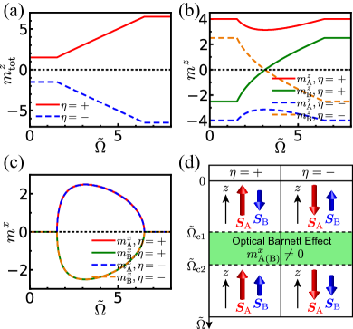
Figure 2: The classical spin configuration that minimizes the energy $\epsilon$ [Eq. (5)]. (a) $m_{\mathrm{tot}}^{z}$, (b) $m_{\mathrm{A(B)}}^{z}$, and (c) $m_{\mathrm{A(B)}}^{x}$ are shown as a function of $\tilde{\Omega}=\hbar\Omega/(z_{0}J)$. The direction of the optical Barnett field depends on the laser chirality $\eta$. The parameters are $S_{\mathrm{A}}=4$, $S_{\mathrm{B}}=5/2$, $D_{\mathrm{A}}/J=17.5\times 10^{-3}$, and $D_{\mathrm{B}}/J=1.5\times 10^{-3}$ following the experimental values for $\mathrm{Er_{3}Fe_{5}O_{12}}$ Ohnuma et al. (2013); Chikazumi (1997); Pearson (1962) ($J=0.2$ meV). The lower and upper critical frequencies are $\tilde{\Omega}_{\mathrm{c1}}=1.54$ and $\tilde{\Omega}_{\mathrm{c2}}=6.49$, respectively. (d) Summary of the optical Barnett effect and the magnetization reversal on the sublattice B for both circular polarization of laser.

III Optomagnonic Barnett effect

In this paper we discuss the formation of the quasiequilibrium magnon BEC provoked by the optical Barnett effect, which we call the optomagnonic Barnett effect. As a platform, we consider the laser application to insulating ferrimagnets (Fig. 1),

$$\mathcal{H}_{0}= J\sum_{\langle i\in\mathrm{A},j\in\mathrm{B}\rangle}\boldsymbol{S}_{\mathrm{A},i}\cdot\boldsymbol{S}_{\mathrm{B},j}$$

$$-D_{\mathrm{A}}\sum_{i\in\mathrm{A}}(S_{\mathrm{A},i}^{z})^{2}-D_{\mathrm{B}}\sum_{j\in\mathrm{B}}(S_{\mathrm{B},j}^{z})^{2},$$ (4)

where $\boldsymbol{S}_{\mathrm{A(B)},i(j)}=(S_{\mathrm{A(B)},i(j)}^{x},S_{\mathrm{A(B)},i(j)}^{y},S_{\mathrm{A(B)},i(j)}^{z})$ represents the spin at the $i(j)$-th site on the sublattice $\mathrm{A(B)}$ having the spin quantum number $S_{\mathrm{A(B)}}$, $J>0$ is the exchange interaction between the nearest neighbor spins $\langle i\in\mathrm{A},j\in\mathrm{B}\rangle$, and $D_{\mathrm{A(B)}}>0$ is the easy-axis single ion anisotropy for the sublattice $\mathrm{A(B)}$ that ensures a magnetic order in the $z$ direction. In the systems with anisotropy, we can realize the dynamical magnetization curve by modulating the laser frequency $\Omega$ slowly enough Takayoshi et al. (2014b), which is the experimental technique called chirping Sato et al. (2013); Kamada et al. (2013).

We remark that in antiferromagnets ($S_{\mathrm{A}}=S_{\mathrm{B}}$) with easy-axis anisotropy, the spin-flop transition happens in the low field regime associated with the Néel magnetic order when the static external field is increased Chow and Keffer (1974). The spin-flop transition is of the first order and the change of the state is drastic. In the case of laser application, the dynamical state cannot follow this sudden change, and the optical Barnett effect does not take place. In ferrimagnets ($S_{\mathrm{A}}\not=S_{\mathrm{B}}$), however, the spin-flop transition is absent Clark and Callen (1968), and that is why we consider ferrimagnets in this paper.

III.1 Classical theory

First we analyze the optical Barnett effect in the classical case. Since the effective Hamiltonian Eq. (2), where $\mathcal{H}_{0}$ is Eq. (4), has the $U(1)$ symmetry, we assume that the spins reside in the $xz$ plane, $\boldsymbol{S}_{\mathrm{A},i}=(m_{\mathrm{A}}^{x},0,m_{\mathrm{A}}^{z})$ and $\boldsymbol{S}_{\mathrm{B},j}=(m_{\mathrm{B}}^{x},0,m_{\mathrm{B}}^{z})$. The classical energy normalized by the number of spins is given as

$$\epsilon=\frac{z_{0}J}{2}\boldsymbol{S}_{\mathrm{A}}\cdot\boldsymbol{S}_{\mathrm{B}}-\frac{D_{\mathrm{A}}}{2}(S_{\mathrm{A}}^{z})^{2}-\frac{D_{\mathrm{B}}}{2}(S_{\mathrm{B}}^{z})^{2}-\eta\frac{\hbar\Omega}{2}(S_{\mathrm{A}}^{z}+S_{\mathrm{B}}^{z}),$$ (5)

where $z_{0}$ is the coordination number. We numerically obtain the classical spin configuration that minimizes the energy [Eq. (5)], and show the result in Fig. 2. Here we consider the cubic lattice with $z_{0}=6$. The magnetization curve induced by the optical Barnett field, i.e., $m_{\mathrm{tot}}^{z}\coloneqq m_{\mathrm{A}}^{z}+m_{\mathrm{B}}^{z}$ as a function of the normalized frequency $\tilde{\Omega}\coloneqq\hbar\Omega/(z_{0}J)$, is shown in Fig. 2(a). When the frequency $\tilde{\Omega}$ is small, the spin configuration is unchanged and aligned along the $z$ direction due to the anisotropy. Above the lower critical frequency $\tilde{\Omega}_{\mathrm{c1}}$, the total magnetization along the $z$ axis starts to grow. In this optical Barnett effect, $m_{\mathrm{tot}}^{z}$ increases continuously and attains full polarization at the upper critical frequency $\tilde{\Omega}_{\mathrm{c2}}$. Fig. 2(b) shows the change of $m_{\mathrm{A}}^{z}$ and $m_{\mathrm{B}}^{z}$ with increasing $\Omega$. This indicates that the spins on the sublattice B are reversed from $-\eta S_{\mathrm{B}}$ to $\eta S_{\mathrm{B}}$. The controllability for the direction of the optical Barnett field by the laser chirality $\eta=\pm$ provides a handle to design optomagnonic functionalities in various magnets, e.g., electron and nuclear spin systems, even paramagnets. From Fig. 2(c), we see that both $m_{\mathrm{A}}^{x}$ and $m_{\mathrm{B}}^{x}$ change continuously and take nonzero value in $\tilde{\Omega}_{\mathrm{c1}}<\tilde{\Omega}<\tilde{\Omega}_{\mathrm{c2}}$.

Those results of the optical Barnett effect and the magnetization reversal in the insulating ferrimagnet are summarized in Fig. 2(d). The explicit form of $\tilde{\Omega}_{\mathrm{c1(c2)}}$ is given in the Appendix B.

III.2 Spin wave theory

The absence of the first order transition, i.e., jump of $m_{\mathrm{tot}}^{z}$, in the vicinity of $\tilde{\Omega}_{\mathrm{c1}}$ and $\tilde{\Omega}_{\mathrm{c2}}$ ensures the validity of the description in terms of the magnon picture. Hence we move to the analysis by the spin wave theory next, and see that $\tilde{\Omega}_{\mathrm{c1}}$ and $\tilde{\Omega}_{\mathrm{c2}}$ become the magnon BEC transition points.

We first consider increasing the frequency $\Omega$ from below $\tilde{\Omega}_{\mathrm{c1}}$, where the ground state has an alternating structure of up and down spins [Figs. 2(b) and 2(d)]. From the spin wave theory, elementary excitations are two kinds of magnons Ohnuma et al. (2013); Nakata et al. (2017b) designated by the index $\sigma=\pm$ having the spin angular momentum $\delta S^{z}=-\eta\sigma 1$. The Hamiltonian [Eqs. (2) and (4)] can be recast into the diagonal form due to the $U(1)$ symmetry as

$${\mathcal{H}}_{\mathrm{eff}}=\sum_{\sigma=\pm,\boldsymbol{k}}(\hbar\omega_{\sigma,\boldsymbol{k}}^{[\alpha]}+\Delta_{\sigma}^{[\alpha]}+\sigma\hbar\Omega)\alpha_{\sigma,\boldsymbol{k}}^{\dagger}\alpha_{\sigma,\boldsymbol{k}},$$ (6)

where $\Delta_{\sigma}^{[\alpha]}+\sigma\hbar\Omega$ is the magnon gap in laser and $\hbar\omega_{\sigma,\boldsymbol{k}}^{[\alpha]}$ is the energy dispersion of the $\sigma$ magnon annihilated (created) by the bosonic operator $\alpha_{\sigma,\boldsymbol{k}}^{(\dagger)}$ with $[\alpha_{\sigma,\boldsymbol{k}},\alpha_{\sigma^{\prime},\boldsymbol{k^{\prime}}}^{\dagger}]=\delta_{\sigma,\sigma^{\prime}}\delta_{{\boldsymbol{k}},\boldsymbol{k^{\prime}}}$. For the details of the calculation and the explicit forms of $\Delta_{\sigma}^{[\alpha]}$ and $\omega_{\sigma,\boldsymbol{k}}^{[\alpha]}$, see the Appendix C. With increasing $\Omega$, the energy band of $\sigma=-$ magnon goes down, while that of $\sigma=+$ magnon goes up due to the $\sigma\hbar\Omega$ term. The former touches the zero energy at

$$\Omega_{\mathrm{BEC1}}\coloneqq\Delta_{-}^{[\alpha]}/\hbar,$$ (7)

and the second order phase transition happens from the proliferation of magnons. This is the quasiequilibrium magnon BEC induced by the optical Barnett field, which we call the optical magnon BEC. $\Omega_{\mathrm{BEC1}}$ coincides with $\Omega_{\mathrm{c1}}$. This optical magnon BEC is the macroscopic coherent state with the transverse magnetization associated with the spontaneous $U(1)$ symmetry breaking , and thus the total magnetization along the $z$ axis grows (Fig. 2). Therefore this optical Barnett effect can be observed as the phenomenon induced by the optical magnon BEC transition, and we refer to this behavior in insulating ferrimagnets especially as the optomagnonic Barnett effect.

Next we consider decreasing the frequency $\Omega$ from above $\tilde{\Omega}_{\mathrm{c2}}$, where spins are full polarized in the ground state [Figs. 2(b) and 2(d)]. Again there are two kinds of magnons designated by the index $\sigma=\pm$ due to $S_{\mathrm{A}}\not=S_{\mathrm{B}}$, but in contrast to the $\Omega_{\mathrm{BEC1}}$ case, both magnons have the same spin angular momentum $\delta S^{z}=-\eta 1$ since spins on both sublattices are polarized in the same direction. We can derive the Hamiltonian in the diagonal form

$${\mathcal{H}}_{\mathrm{eff}}=\sum_{\sigma=\pm,\boldsymbol{k}}(\hbar\omega_{\sigma,\boldsymbol{k}}^{[\beta]}+\Delta_{\sigma}^{[\beta]}+\hbar\Omega)\beta_{\sigma,\boldsymbol{k}}^{\dagger}\beta_{\sigma,\boldsymbol{k}},$$ (8)

where $\Delta_{\sigma}^{[\beta]}+\hbar\Omega$ is the magnon gap in laser and $\hbar\omega_{\sigma,\boldsymbol{k}}^{[\beta]}$ is the energy dispersion of the $\sigma$ magnon annihilated (created) by the bosonic operator $\beta_{\sigma,\boldsymbol{k}}^{(\dagger)}$ with $[\beta_{\sigma,\boldsymbol{k}},\beta_{\sigma^{\prime},\boldsymbol{k^{\prime}}}^{\dagger}]=\delta_{\sigma,\sigma^{\prime}}\delta_{{\boldsymbol{k}},\boldsymbol{k^{\prime}}}$. For the explicit forms of $\Delta_{\sigma}^{[\beta]}(\leq 0)$ and $\omega_{\sigma,\boldsymbol{k}}^{[\beta]}$, see the Appendix C. With decreasing $\Omega$, the energy band of both $\sigma=\pm$ magnon goes down due to the $\hbar\Omega$ term, and the lower band touches the zero energy at

$$\Omega_{\mathrm{BEC2}}\coloneqq-\Delta_{-}^{[\beta]}/\hbar.$$ (9)

In the same way as the $\Omega_{\mathrm{BEC1}}$ case, the second order phase transition happens at $\Omega_{\mathrm{BEC2}}$ and magnons form the quasiequilibrium BEC. $\Omega_{\mathrm{BEC2}}$ coincides with $\Omega_{\mathrm{c2}}$. Thus the optomagnonic Barnett effect is induced in the regime $\Omega_{\mathrm{BEC1}}<\Omega<\Omega_{\mathrm{BEC2}}$.

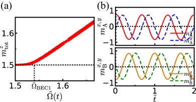
Figure 3: The magnetization dynamics for the laser chirality $\eta=+$ calculated by the TDMF theory. Time evolution of (a) $m_{\mathrm{tot}}^{z}$ and (b) $xy$ components of sublattice magnetization are shown. The result clearly shows the condensation of magnons and the precession of magnetization around the $z$ axis.

III.3 Magnetization dynamics

Finally, to investigate the dynamics of the optomagnonic Barnett effect, we numerically solve the equation of motion derived from the time-dependent mean field (TDMF) theory and calculate the time evolution of sublattice magnetization (Appendix D). The TDMF theory can well capture the magnetization dynamics Takayoshi et al. (2019). The parameters are the same in Fig. 2, $S_{\mathrm{A}}=4$, $S_{\mathrm{B}}=5/2$, $z_{0}=6$, $D_{\mathrm{A}}/J=17.5\times 10^{-3}$, and $D_{\mathrm{B}}/J=1.5\times 10^{-3}$. We use the laser with polarization $\eta=+$ represented as $B_{0}(\cos\vartheta(t),\sin\vartheta(t),0)$, where the amplitude is $B_{0}/J=0.2$ and the frequency is chirped as $\vartheta(t)=\Omega_{0}t+vt^{2}/2$ with the normalized chirping speed $\hbar^{2}v/J^{2}=10^{-5}$ and $\hbar\Omega_{0}/J=9$. The normalized instantaneous frequency is defined as $\tilde{\Omega}(t)\coloneqq\hbar(d\vartheta(t)/dt)/(z_{0}J)=(\hbar\Omega_{0}+\hbar vt)/(z_{0}J)$. We calculate the dynamics in the time region $0\leq tJ/\hbar\leq 10^{5}$, which corresponds to $1.5\leq\tilde{\Omega}(t)\leq 1.66$ in the frequency regime. Figure 3(a) shows the time evolution of $m_{\mathrm{tot}}^{z}=m_{\mathrm{A}}^{z}+m_{\mathrm{B}}^{z}$. We can see that $m_{\mathrm{tot}}^{z}$ starts to grow from $S_{\mathrm{A}}-S_{\mathrm{B}}=3/2$ when $\tilde{\Omega}(t)$ exceeds $\tilde{\Omega}_{\mathrm{BEC1}}=1.54$. In Fig. 3(b), we show the time evolution for the $xy$ components of sublattice magnetization around $\tilde{\Omega}(t)=1.6$ in the time interval of $0\leq\tilde{t}\leq 2$, where $\tilde{t}\coloneqq tJ/\hbar-6\times 10^{4}$ is the normalized time. The result clearly shows that magnetization on both sublattices precesses around the $z$ axis with the instantaneous frequency, same as the laser $\tilde{\Omega}(t)$, and the $xy$ components of A and B sublattice magnetization are in the opposite direction. The period of this spin precession is $O(1)$ ps.

IV Experimental feasibility

We make an estimate for an insulating ferrimagnet $\mathrm{Er_{3}Fe_{5}O_{12}}$ Ohnuma et al. (2013); Chikazumi (1997); Pearson (1962), and give the magnetization curve and the experimental parameter values in Fig. 2 and its caption, respectively. We find that the magnon BEC transition points are $\Omega_{\mathrm{BEC1}}=1.85$ THz and $\Omega_{\mathrm{BEC2}}=7.8$ THz , and the optical Barnett field amounts to $\mathcal{B}=O(10)$ T for $\Omega=O(1)$ THz. Our proposal is within the experimental reach with current device and measurement technologies, e.g., nuclear magnetic resonance Chudo et al. (2014); Arabgol and Sleator (2019); Lee et al. (2006) for the optical Barnett field, magneto-optical Kerr effect Qiu and Bader (2000) for the magnetization reversal in the optical Barnett effect, Brillouin light scattering Demokritov et al. (2006) for the optical magnon BEC, and terahertz spectroscopy Yamaguchi et al. (2013); Mikhaylovskiy et al. (2014) for the spin dynamics of the order of picoseconds. Since magnons are induced by laser and not by thermal fluctuation in the present setup, our findings are realizable at low temperature Kosen et al. (2018); Tabuchi et al. (2014, 2015); Prasai et al. (2017) where phonon degrees of freedom cease to work.

We emphasize the importance of modulating the laser frequency adiabatically Takayoshi et al. (2014a, b) by the chirping technique Sato et al. (2013); Kamada et al. (2013). Otherwise, the deviation from the magnetization curve happens due to a nonadiabatic transition from the Landau-Zener tunneling Landau (1932); Zener (1934). To avoid this effect, a large magnetic anisotropy and a strong laser field is advantageous Takayoshi et al. (2014a). In addition, the laser chirping suppresses heating effects drastically.

V Discussion

First, the laser application without chirping can be studied by the Floquet theory with inverse frequency expansion Bukov et al. (2015); Sato et al. (2016); Nakata et al. (2019). This analysis also supports the generation of the optical Barnett field in the high frequency regime (Appendix E).

Second, we remark that the optical Barnett field through the chirping is proportional to the laser frequency $\mathcal{B}\propto\Omega$ Takayoshi et al. (2014a, b). Hence $\Omega=O(1)$ THz amounts to $\mathcal{B}=O(10)$ T, which provides a platform to explore the phenomena at high magnetic field $O(10)$ T or more in the tabletop setup.

Third, optomagnonic cavities for implementing coherent photon-magnon coupling have been theoretically studied in Refs. Pantazopoulos et al. (2017, 2018, 2019); Pantazopoulos and Stefanou (2019, 2020).

Last, as an application of the optomagnonic Barnett effect, it will be intriguing to investigate the magnon Josephson effect in a junction Nakata et al. (2014); Troncoso and Nunez (2014). We leave it for a future study.

VI Conclusion

We applied the optical Barnett effect to insulating ferrimagnets and showed that quasiequilibrium magnon BEC can be realized using the spin-wave theory. This optomagnonic Barnett effect provides an access to coherent magnons in the frequency regime of the order of terahertz, which is much faster time scale than the conventional microwave pumping. Our findings are expected to become a building block for the application to ultrafast spin transport.

Appendix A Effective static Hamiltonian

In this section starting from the time-periodic Hamiltonian

$$\mathcal{H}(t)=\mathcal{H}_{0}-B_{0}[S_{\mathrm{tot}}^{x}\cos(\Omega t)+\eta S_{\mathrm{tot}}^{y}\sin(\Omega t)],$$ (10)

we derive the effective static Hamiltonian Eq. (2) in the main text. We apply the time-dependent unitary transform,

$$U\coloneqq e^{i\eta\Omega tS_{\mathrm{tot}}^{z}},$$ (11)

to $\mathcal{H}(t)$ as

$$\mathcal{H}(t) \to U[\mathcal{H}(t)-i\hbar\partial_{t}]U^{-1}\eqqcolon\mathcal{H}_{\mathrm{eff}}.$$ (12)

Then we obtain the effective static Hamiltonian as

$$\mathcal{H}_{\mathrm{eff}}=\mathcal{H}_{0}-\eta\hbar\Omega S_{\mathrm{tot}}^{z}-B_{0}S_{\mathrm{tot}}^{x}.$$ (13)

In the case of weak laser field $B_{0}\ll\hbar\Omega$, the $B_{0}S_{\mathrm{tot}}^{x}$ term is negligibly small. Thus we reach the effective static Hamiltonian Eq. (2) in the main text.

Appendix B Classical theory

In this section, we derive the lower (upper) critical frequency $\Omega_{\mathrm{c1(c2)}}$. The classical spin configuration is determined in the way that the energy

$$\epsilon=\frac{z_{0}J}{2}\boldsymbol{S}_{\mathrm{A}}\cdot\boldsymbol{S}_{\mathrm{B}}-\frac{D_{\mathrm{A}}}{2}(S_{\mathrm{A}}^{z})^{2}-\frac{D_{\mathrm{B}}}{2}(S_{\mathrm{B}}^{z})^{2}-\eta\frac{\hbar\Omega}{2}(S_{\mathrm{A}}^{z}+S_{\mathrm{B}}^{z})$$ (14)

takes minimum. Since Eq. (14) has the $U(1)$ symmetry, we assume that $\boldsymbol{S}_{\mathrm{A}}$ and $\boldsymbol{S}_{\mathrm{B}}$ are in the $xz$ plane. We parametrize the spins as $\boldsymbol{S}_{\mathrm{A}}=(S_{\mathrm{A}}\sin\theta_{\mathrm{A}},0,\eta S_{\mathrm{A}}\cos\theta_{\mathrm{A}})$ and $\boldsymbol{S}_{\mathrm{B}}=(-S_{\mathrm{B}}\sin\theta_{\mathrm{B}},0,\eta S_{\mathrm{B}}\cos\theta_{\mathrm{B}})$. Then Eq. (14) can be rewritten as

$$\epsilon=\frac{z_{0}JS_{\mathrm{A}}S_{\mathrm{B}}}{2}\cos(\theta_{\mathrm{A}}+\theta_{\mathrm{B}})-\frac{D_{\mathrm{A}}S_{\mathrm{A}}^{2}}{2}\cos^{2}\theta_{\mathrm{A}}-\frac{D_{\mathrm{B}}S_{\mathrm{B}}^{2}}{2}\cos^{2}\theta_{\mathrm{B}}-\frac{\hbar\Omega}{2}(S_{\mathrm{A}}\cos\theta_{\mathrm{A}}+S_{\mathrm{B}}\cos\theta_{\mathrm{B}}).$$ (15)

From the conditions for the energy minimum, $\partial\epsilon/\partial\theta_{\mathrm{A}}=0$ and $\partial\epsilon/\partial\theta_{\mathrm{B}}=0$, we obtain

$$-z_{0}JS_{\mathrm{B}}\sin(\theta_{\mathrm{A}}+\theta_{\mathrm{B}})+2D_{\mathrm{A}}S_{\mathrm{A}}\cos\theta_{\mathrm{A}}\sin\theta_{\mathrm{A}}+\hbar\Omega\sin\theta_{\mathrm{A}}= 0,$$ (16)

$$-z_{0}JS_{\mathrm{A}}\sin(\theta_{\mathrm{A}}+\theta_{\mathrm{B}})+2D_{\mathrm{B}}S_{\mathrm{B}}\cos\theta_{\mathrm{B}}\sin\theta_{\mathrm{B}}+\hbar\Omega\sin\theta_{\mathrm{B}}= 0.$$ (17)

B.1 Around $\Omega=\Omega_{\mathrm{c}1}$

We consider the frequency just above $\Omega_{\mathrm{c}1}$, where $\sin\theta_{\mathrm{A}}\simeq\theta_{\mathrm{A}}$, $\sin\theta_{\mathrm{B}}\simeq\pi-\theta_{\mathrm{B}}$, $\cos\theta_{\mathrm{A}}\simeq 1$, $\cos\theta_{\mathrm{B}}\simeq-1$, $\theta_{\mathrm{A}}\neq 0$, and $\pi-\theta_{\mathrm{B}}\neq 0$. Then Eqs. (16) and (17) become

$$-z_{0}JS_{\mathrm{B}}(-\theta_{\mathrm{A}}+\pi-\theta_{\mathrm{B}})+2D_{\mathrm{A}}S_{\mathrm{A}}\theta_{\mathrm{A}}+\hbar\Omega_{\mathrm{c}1}\theta_{\mathrm{A}}=0\Leftrightarrow z_{0}JS_{\mathrm{B}}(\pi-\theta_{\mathrm{B}})/\theta_{\mathrm{A}}=z_{0}JS_{\mathrm{B}}+2D_{\mathrm{A}}S_{\mathrm{A}}+\hbar\Omega_{\mathrm{c}1},$$

$$-z_{0}JS_{\mathrm{A}}(-\theta_{\mathrm{A}}+\pi-\theta_{\mathrm{B}})-2D_{\mathrm{B}}S_{\mathrm{B}}(\pi-\theta_{\mathrm{B}})+\hbar\Omega_{\mathrm{c}1}(\pi-\theta_{\mathrm{B}})=0\Leftrightarrow z_{0}JS_{\mathrm{A}}\theta_{\mathrm{A}}/(\pi-\theta_{\mathrm{B}})=z_{0}JS_{\mathrm{A}}+2D_{\mathrm{B}}S_{\mathrm{B}}-\hbar\Omega_{\mathrm{c}1}.$$

Thus

$$(\hbar\Omega_{\mathrm{c}1}+z_{0}JS_{\mathrm{B}}+2D_{\mathrm{A}}S_{\mathrm{A}})(\hbar\Omega_{\mathrm{c}1}-z_{0}JS_{\mathrm{A}}-2D_{\mathrm{B}}S_{\mathrm{B}})=-z_{0}^{2}J^{2}S_{\mathrm{A}}S_{\mathrm{B}}$$

$$\Leftrightarrow [\{\hbar\Omega_{\mathrm{c}1}-z_{0}J(S_{\mathrm{A}}-S_{\mathrm{B}})/2+D_{\mathrm{A}}S_{\mathrm{A}}-D_{\mathrm{B}}S_{\mathrm{B}}\}+\{z_{0}J(S_{\mathrm{A}}+S_{\mathrm{B}})/2+D_{\mathrm{A}}S_{\mathrm{A}}+D_{\mathrm{B}}S_{\mathrm{B}}\}]$$

$$\times[\{\hbar\Omega_{\mathrm{c}1}-z_{0}J(S_{\mathrm{A}}-S_{\mathrm{B}})/2+D_{\mathrm{A}}S_{\mathrm{A}}-D_{\mathrm{B}}S_{\mathrm{B}}\}-\{z_{0}J(S_{\mathrm{A}}+S_{\mathrm{B}})/2+D_{\mathrm{A}}S_{\mathrm{A}}+D_{\mathrm{B}}S_{\mathrm{B}}\}]=-z_{0}^{2}J^{2}S_{\mathrm{A}}S_{\mathrm{B}}$$

$$\Leftrightarrow \hbar\Omega_{\mathrm{c}1}=z_{0}J(S_{\mathrm{A}}-S_{\mathrm{B}})/2-D_{\mathrm{A}}S_{\mathrm{A}}+D_{\mathrm{B}}S_{\mathrm{B}}\pm\sqrt{-z_{0}^{2}J^{2}S_{\mathrm{A}}S_{\mathrm{B}}+[z_{0}J(S_{\mathrm{A}}+S_{\mathrm{B}})/2+D_{\mathrm{A}}S_{\mathrm{A}}+D_{\mathrm{B}}S_{\mathrm{B}}]^{2}}.$$

From $\Omega_{\mathrm{c}1}>0$, we obtain

$$\hbar\Omega_{\mathrm{c}1}=z_{0}J(S_{\mathrm{A}}-S_{\mathrm{B}})/2-D_{\mathrm{A}}S_{\mathrm{A}}+D_{\mathrm{B}}S_{\mathrm{B}}+\sqrt{-z_{0}^{2}J^{2}S_{\mathrm{A}}S_{\mathrm{B}}+[z_{0}J(S_{\mathrm{A}}+S_{\mathrm{B}})/2+D_{\mathrm{A}}S_{\mathrm{A}}+D_{\mathrm{B}}S_{\mathrm{B}}]^{2}}.$$ (18)

B.2 Around $\Omega=\Omega_{\mathrm{c}2}$

We consider the frequency just below $\Omega_{\mathrm{c}2}$, where $\sin\theta_{\mathrm{A}}\simeq\theta_{\mathrm{A}}$, $\sin\theta_{\mathrm{B}}\simeq\theta_{\mathrm{B}}$, $\cos\theta_{\mathrm{A}}\simeq 1$, $\cos\theta_{\mathrm{B}}\simeq 1$, $\theta_{\mathrm{A}}\neq 0$, and $\theta_{\mathrm{B}}\neq 0$. Then Eqs. (16) and (17) become

$$-z_{0}JS_{\mathrm{B}}(\theta_{\mathrm{A}}+\theta_{\mathrm{B}})+2D_{\mathrm{A}}S_{\mathrm{A}}\theta_{\mathrm{A}}+\hbar\Omega_{\mathrm{c}2}\theta_{\mathrm{A}}=0\Leftrightarrow z_{0}JS_{\mathrm{B}}\theta_{\mathrm{B}}/\theta_{\mathrm{A}}=-z_{0}JS_{\mathrm{B}}+2D_{\mathrm{A}}S_{\mathrm{A}}+\hbar\Omega_{\mathrm{c}2},$$

$$-z_{0}JS_{\mathrm{A}}(\theta_{\mathrm{A}}+\theta_{\mathrm{B}})+2D_{\mathrm{B}}S_{\mathrm{B}}\theta_{\mathrm{B}}+\hbar\Omega_{\mathrm{c}2}\theta_{\mathrm{B}}=0\Leftrightarrow z_{0}JS_{\mathrm{A}}\theta_{\mathrm{A}}/\theta_{\mathrm{B}}=-z_{0}JS_{\mathrm{A}}+2D_{\mathrm{B}}S_{\mathrm{B}}+\hbar\Omega_{\mathrm{c}2}.$$

Thus

$$(\hbar\Omega_{\mathrm{c}2}-z_{0}JS_{\mathrm{B}}+2D_{\mathrm{A}}S_{\mathrm{A}})(\hbar\Omega_{\mathrm{c}2}-z_{0}JS_{\mathrm{A}}+2D_{\mathrm{B}}S_{\mathrm{B}})=z_{0}^{2}J^{2}S_{\mathrm{A}}S_{\mathrm{B}}$$

$$\Leftrightarrow [\{\hbar\Omega_{\mathrm{c}2}-z_{0}J(S_{\mathrm{A}}+S_{\mathrm{B}})/2+D_{\mathrm{A}}S_{\mathrm{A}}+D_{\mathrm{B}}S_{\mathrm{B}}\}+\{z_{0}J(S_{\mathrm{A}}-S_{\mathrm{B}})/2+D_{\mathrm{A}}S_{\mathrm{A}}-D_{\mathrm{B}}S_{\mathrm{B}}\}]$$

$$\times[\{\hbar\Omega_{\mathrm{c}2}-z_{0}J(S_{\mathrm{A}}+S_{\mathrm{B}})/2+D_{\mathrm{A}}S_{\mathrm{A}}+D_{\mathrm{B}}S_{\mathrm{B}}\}-\{z_{0}J(S_{\mathrm{A}}-S_{\mathrm{B}})/2+D_{\mathrm{A}}S_{\mathrm{A}}-D_{\mathrm{B}}S_{\mathrm{B}}\}]=z_{0}^{2}J^{2}S_{\mathrm{A}}S_{\mathrm{B}}$$

$$\Leftrightarrow \hbar\Omega_{\mathrm{c}2}=z_{0}J(S_{\mathrm{A}}+S_{\mathrm{B}})/2-D_{\mathrm{A}}S_{\mathrm{A}}-D_{\mathrm{B}}S_{\mathrm{B}}\pm\sqrt{z_{0}^{2}J^{2}S_{\mathrm{A}}S_{\mathrm{B}}+[z_{0}J(S_{\mathrm{A}}-S_{\mathrm{B}})/2+D_{\mathrm{A}}S_{\mathrm{A}}-D_{\mathrm{B}}S_{\mathrm{B}}]^{2}}.$$

From $\Omega_{\mathrm{c}2}>0$, we obtain

$$\hbar\Omega_{\mathrm{c}2}=z_{0}J(S_{\mathrm{A}}+S_{\mathrm{B}})/2-D_{\mathrm{A}}S_{\mathrm{A}}-D_{\mathrm{B}}S_{\mathrm{B}}+\sqrt{z_{0}^{2}J^{2}S_{\mathrm{A}}S_{\mathrm{B}}+[z_{0}J(S_{\mathrm{A}}-S_{\mathrm{B}})/2+D_{\mathrm{A}}S_{\mathrm{A}}-D_{\mathrm{B}}S_{\mathrm{B}}]^{2}}.$$ (19)

Appendix C Spin wave theory

In this section, we derive the magnon BEC transition point $\Omega_{\mathrm{BEC1(BEC2)}}$ and see that it coincides with the lower (upper) critical frequency ${\Omega}_{\mathrm{c1(c2)}}$. We consider the system

$${\mathcal{H}}_{\mathrm{eff}}=J\sum_{\langle i\in\mathrm{A},j\in\mathrm{B}\rangle}\boldsymbol{S}_{\mathrm{A},i}\cdot\boldsymbol{S}_{\mathrm{B},j}-D_{\mathrm{A}}\sum_{i\in\mathrm{A}}(S_{\mathrm{A},i}^{z})^{2}-D_{\mathrm{B}}\sum_{j\in\mathrm{B}}(S_{\mathrm{B},j}^{z})^{2}-\eta\hbar\Omega\Big{(}\sum_{i\in\mathrm{A}}S_{\mathrm{A},i}^{z}+\sum_{j\in\mathrm{B}}S_{\mathrm{B},j}^{z}\Big{)}.$$ (20)

The boundary condition is periodic, and the number of sites is $N$; $N/2$ sites for the A and B sublattice.

C.1 Around $\Omega=\Omega_{\mathrm{BEC}1}$

The ground state is ferrimagnetic $\boldsymbol{S}_{\mathrm{A}}=(0,0,\eta S_{\mathrm{A}})$ and $\boldsymbol{S}_{\mathrm{B}}=(0,0,-\eta S_{\mathrm{B}})$. We perform the Holstein-Primakoff transformation,

$$\eta S_{\mathrm{A},i}^{z}=S_{\mathrm{A}}-n_{\mathrm{A},i},\quad S_{\mathrm{A},i}^{x}+\eta iS_{\mathrm{A},i}^{y}=\sqrt{2S_{\mathrm{A}}}\Big{(}1-\frac{n_{\mathrm{A},i}}{2S_{\mathrm{A}}}\Big{)}^{1/2}b_{\mathrm{A},i},\quad S_{\mathrm{A},i}^{x}-\eta iS_{\mathrm{A},i}^{y}=\sqrt{2S_{\mathrm{A}}}b_{\mathrm{A},i}^{\dagger}\Big{(}1-\frac{n_{\mathrm{A},i}}{2S_{\mathrm{A}}}\Big{)}^{1/2},$$

$$\eta S_{\mathrm{B},j}^{z}=-S_{\mathrm{B}}+n_{\mathrm{B},j},\quad S_{\mathrm{B},j}^{x}+\eta iS_{\mathrm{B},j}^{y}=\sqrt{2S_{\mathrm{B}}}b_{\mathrm{B},j}^{\dagger}\Big{(}1-\frac{n_{\mathrm{B},j}}{2S_{\mathrm{B}}}\Big{)}^{1/2},S_{\mathrm{B},j}^{x}-\eta iS_{\mathrm{B},j}^{y}=\sqrt{2S_{\mathrm{B}}}\Big{(}1-\frac{n_{\mathrm{B},j}}{2S_{\mathrm{B}}}\Big{)}^{1/2}b_{\mathrm{B},j},\quad$$

where $b_{j}^{\dagger}$ and $b_{j}$ are creation and annihilation operators for bosons (magnons), and $n_{(\mathrm{A},\mathrm{B}),j}\equiv b_{(\mathrm{A},\mathrm{B}),j}^{\dagger}b_{(\mathrm{A},\mathrm{B}),j}$ is the number operator. We make an expansion and retain up to the second order in terms of $b$ and $b^{\dagger}$,

$$\eta S_{\mathrm{A},i}^{z}=S_{\mathrm{A}}-n_{\mathrm{A},i},\quad S_{\mathrm{A},i}^{x}+\eta iS_{\mathrm{A},i}^{y}=\sqrt{2S_{\mathrm{A}}}b_{\mathrm{A},i},\quad S_{\mathrm{A},i}^{x}-\eta iS_{\mathrm{A},i}^{y}=\sqrt{2S_{\mathrm{A}}}b_{\mathrm{A},i}^{\dagger},$$

$$\eta S_{\mathrm{B},j}^{z}=-S_{\mathrm{B}}+n_{\mathrm{B},j},\quad S_{\mathrm{B},j}^{x}+\eta iS_{\mathrm{B},j}^{y}=\sqrt{2S_{\mathrm{B}}}b_{\mathrm{B},j}^{\dagger},\quad S_{\mathrm{B},j}^{x}-\eta iS_{\mathrm{B},j}^{y}=\sqrt{2S_{\mathrm{B}}}b_{\mathrm{B},j}.$$

Using magnon operators, the Hamiltonian (20) is rewritten as

$${\mathcal{H}}_{\mathrm{eff}}= J\sqrt{S_{\mathrm{A}}S_{\mathrm{B}}}\sum_{\langle i\in\mathrm{A},j\in\mathrm{B}\rangle}(b_{\mathrm{A},i}b_{\mathrm{B},j}+\mathrm{H.c.})+z_{0}JS_{\mathrm{B}}\sum_{i\in\mathrm{A}}n_{\mathrm{A},i}+z_{0}JS_{\mathrm{A}}\sum_{j\in\mathrm{B}}n_{\mathrm{B},j}$$

$$+2D_{\mathrm{A}}S_{\mathrm{A}}\sum_{i\in\mathrm{A}}n_{\mathrm{A},i}+2D_{\mathrm{B}}S_{\mathrm{B}}\sum_{j\in\mathrm{B}}n_{\mathrm{B},j}+\hbar\Omega\Big{(}\sum_{i\in\mathrm{A}}n_{\mathrm{A},i}-\sum_{j\in\mathrm{B}}n_{\mathrm{B},j}\Big{)},$$ (21)

where the constant terms are dropped. We consider the cubic lattice and the coordination number is $z_{0}=6$. After the Fourier transform

$$b_{\mathrm{A},\boldsymbol{k}}=\sqrt{\frac{2}{N}}\sum_{i\in\mathrm{A}}e^{-i\boldsymbol{k}\cdot\boldsymbol{r}_{i}}b_{\mathrm{A},i},\quad b_{\mathrm{A},\boldsymbol{k}}^{\dagger}=\sqrt{\frac{2}{N}}\sum_{i\in\mathrm{A}}e^{i\boldsymbol{k}\cdot\boldsymbol{r}_{i}}b_{\mathrm{A},i}^{\dagger},\quad n_{\mathrm{A},\boldsymbol{k}}=b_{\mathrm{A},\boldsymbol{k}}^{\dagger}b_{\mathrm{A},\boldsymbol{k}},$$

$$b_{\mathrm{B},\boldsymbol{k}}=\sqrt{\frac{2}{N}}\sum_{i\in\mathrm{B}}e^{i\boldsymbol{k}\cdot\boldsymbol{r}_{i}}b_{\mathrm{B},i},\quad b_{\mathrm{B},\boldsymbol{k}}^{\dagger}=\sqrt{\frac{2}{N}}\sum_{i\in\mathrm{B}}e^{-i\boldsymbol{k}\cdot\boldsymbol{r}_{i}}b_{\mathrm{B},i}^{\dagger},\quad n_{\mathrm{B},\boldsymbol{k}}=b_{\mathrm{B},\boldsymbol{k}}^{\dagger}b_{\mathrm{B},\boldsymbol{k}},$$

($\boldsymbol{r}_{i}$ is the positional vector), we obtain

$${\mathcal{H}}_{\mathrm{eff}}= J\sqrt{S_{\mathrm{A}}S_{\mathrm{B}}}\sum_{\boldsymbol{k}}2[\cos(k_{x}a_{0})+\cos(k_{y}a_{0})+\cos(k_{z}a_{0})](b_{\mathrm{A},\boldsymbol{k}}b_{\mathrm{B},\boldsymbol{k}}+\mathrm{H.c.})$$

$$+(z_{0}JS_{\mathrm{B}}+2D_{\mathrm{A}}S_{\mathrm{A}}+\hbar\Omega)\sum_{\boldsymbol{k}}n_{\mathrm{A},\boldsymbol{k}}+(z_{0}JS_{\mathrm{A}}+2D_{\mathrm{B}}S_{\mathrm{B}}-\hbar\Omega)\sum_{\boldsymbol{k}}n_{\mathrm{B},\boldsymbol{k}},$$

where $a_{0}$ is the lattice constant. We perform the Bogoliubov transformation

$$\begin{pmatrix}\alpha_{+,\boldsymbol{k}}\\ \alpha_{-,\boldsymbol{k}}^{\dagger}\end{pmatrix}=\begin{pmatrix}\cosh\theta_{\boldsymbol{k}}&\sinh\theta_{\boldsymbol{k}}\\ \sinh\theta_{\boldsymbol{k}}&\cosh\theta_{\boldsymbol{k}}\end{pmatrix}\begin{pmatrix}b_{\mathrm{A},\boldsymbol{k}}\\ b_{\mathrm{B},\boldsymbol{k}}^{\dagger}\end{pmatrix},$$

with the angle

$$\tanh 2\theta_{\boldsymbol{k}}=\frac{2f(\boldsymbol{k})}{C_{1}+C_{2}},$$

where

$$f(\boldsymbol{k})= 2J\sqrt{S_{\mathrm{A}}S_{\mathrm{B}}}[\cos(k_{x}a_{0})+\cos(k_{y}a_{0})+\cos(k_{z}a_{0})],$$

$$C_{1}= z_{0}JS_{\mathrm{B}}+2D_{\mathrm{A}}S_{\mathrm{A}}+\hbar\Omega,$$

$$C_{2}= z_{0}JS_{\mathrm{A}}+2D_{\mathrm{B}}S_{\mathrm{B}}-\hbar\Omega.$$

Then the Hamiltonian becomes

$${\mathcal{H}}_{\mathrm{eff}}= \sum_{k}\Big{(}-f(\boldsymbol{k})\sinh 2\theta_{\boldsymbol{k}}+\frac{C_{1}-C_{2}}{2}+\frac{C_{1}+C_{2}}{2}\cosh 2\theta_{\boldsymbol{k}}\Big{)}\alpha_{+,\boldsymbol{k}}^{\dagger}\alpha_{+,\boldsymbol{k}}$$

$$+\sum_{k}\Big{(}-f(\boldsymbol{k})\sinh 2\theta_{\boldsymbol{k}}-\frac{C_{1}-C_{2}}{2}+\frac{C_{1}+C_{2}}{2}\cosh 2\theta_{\boldsymbol{k}}\Big{)}\alpha_{-,\boldsymbol{k}}^{\dagger}\alpha_{-,\boldsymbol{k}}$$

$$= \sum_{k}\Big{[}\frac{C_{1}-C_{2}}{2}+\sqrt{-f(\boldsymbol{k})^{2}+\Big{(}\frac{C_{1}+C_{2}}{2}\Big{)}^{2}}\Big{]}\alpha_{+,\boldsymbol{k}}^{\dagger}\alpha_{+,\boldsymbol{k}}$$

$$+\sum_{k}\Big{[}-\frac{C_{1}-C_{2}}{2}+\sqrt{-f(\boldsymbol{k})^{2}+\Big{(}\frac{C_{1}+C_{2}}{2}\Big{)}^{2}}\Big{]}\alpha_{-,\boldsymbol{k}}^{\dagger}\alpha_{-,\boldsymbol{k}},$$ (22)

where the constant terms are dropped. We can rewrite the Hamiltonian in the form

$${\mathcal{H}}_{\mathrm{eff}}=\sum_{\sigma=\pm,\boldsymbol{k}}(\hbar\omega_{\sigma,\boldsymbol{k}}^{[\alpha]}+\Delta_{\sigma}^{[\alpha]}+\sigma\hbar\Omega)\alpha_{\sigma,\boldsymbol{k}}^{\dagger}\alpha_{\sigma,\boldsymbol{k}},$$ (23)

where $\hbar\omega_{\sigma,\boldsymbol{k}}^{[\alpha]}$ is the energy dispersion and $\Delta_{\sigma}^{[\alpha]}+\sigma\hbar\Omega$ is the magnon gap in laser represented as

$$\hbar\omega_{\pm,\boldsymbol{k}}^{[\alpha]}= \sqrt{-f(\boldsymbol{k})^{2}+[3J(S_{\mathrm{A}}+S_{\mathrm{B}})+D_{\mathrm{A}}S_{\mathrm{A}}+D_{\mathrm{B}}S_{\mathrm{B}}]^{2}}-\sqrt{-f(\boldsymbol{0})^{2}+[3J(S_{\mathrm{A}}+S_{\mathrm{B}})+D_{\mathrm{A}}S_{\mathrm{A}}+D_{\mathrm{B}}S_{\mathrm{B}}]^{2}},$$

$$\Delta_{\pm}^{[\alpha]}= \mp[3J(S_{\mathrm{A}}-S_{\mathrm{B}})-D_{\mathrm{A}}S_{\mathrm{A}}+D_{\mathrm{B}}S_{\mathrm{B}}]+\sqrt{-f(\boldsymbol{0})^{2}+[3J(S_{\mathrm{A}}+S_{\mathrm{B}})+D_{\mathrm{A}}S_{\mathrm{A}}+D_{\mathrm{B}}S_{\mathrm{B}}]^{2}},$$

noting that $f(\boldsymbol{k})$ takes the maximum at $\boldsymbol{k}=\boldsymbol{0}$. Therefore, when $\Omega$ is increased from the small value, the magnon created by $\alpha_{-,\boldsymbol{k}=\boldsymbol{0}}^{\dagger}$ condensates at

$$\hbar\Omega_{\mathrm{BEC1}}=\Delta_{-}^{[\alpha]}=3J(S_{\mathrm{A}}-S_{\mathrm{B}})-D_{\mathrm{A}}S_{\mathrm{A}}+D_{\mathrm{B}}S_{\mathrm{B}}+\sqrt{-36J^{2}S_{\mathrm{A}}S_{\mathrm{B}}+[3J(S_{\mathrm{A}}+S_{\mathrm{B}})+D_{\mathrm{A}}S_{\mathrm{A}}+D_{\mathrm{B}}S_{\mathrm{B}}]^{2}},$$ (24)

which agrees with $\hbar\Omega_{\mathrm{c1}}$ [Eq. (18)].

C.2 Around $\Omega=\Omega_{\mathrm{BEC}2}$

The ground state is ferromagnetic $\boldsymbol{S}_{\mathrm{A}}=(0,0,\eta S_{\mathrm{A}})$ and $\boldsymbol{S}_{\mathrm{B}}=(0,0,\eta S_{\mathrm{B}})$. We perform the Holstein-Primakoff transformation,

$$\eta S_{\mathrm{A},i}^{z}=S_{\mathrm{A}}-n_{\mathrm{A},i},\quad S_{\mathrm{A},i}^{x}+\eta iS_{\mathrm{A},i}^{y}=\sqrt{2S_{\mathrm{A}}}\Big{(}1-\frac{n_{\mathrm{A},i}}{2S_{\mathrm{A}}}\Big{)}^{1/2}b_{\mathrm{A},i},\quad S_{\mathrm{A},i}^{x}-\eta iS_{\mathrm{A},i}^{y}=\sqrt{2S_{\mathrm{A}}}b_{\mathrm{A},i}^{\dagger}\Big{(}1-\frac{n_{\mathrm{A},i}}{2S_{\mathrm{A}}}\Big{)}^{1/2},$$

$$\eta S_{\mathrm{B},j}^{z}=S_{\mathrm{B}}-n_{\mathrm{B},j},\quad S_{\mathrm{B},j}^{x}+\eta iS_{\mathrm{B},j}^{y}=\sqrt{2S_{\mathrm{B}}}\Big{(}1-\frac{n_{\mathrm{B},j}}{2S_{\mathrm{B}}}\Big{)}^{1/2}b_{\mathrm{B},j},\quad S_{\mathrm{B},j}^{x}-\eta iS_{\mathrm{B},j}^{y}=\sqrt{2S_{\mathrm{B}}}b_{\mathrm{B},j}^{\dagger}\Big{(}1-\frac{n_{\mathrm{B},j}}{2S_{\mathrm{B}}}\Big{)}^{1/2},$$

where $b_{j}^{\dagger}$ and $b_{j}$ are creation and annihilation operators for bosons (magnons), and $n_{(\mathrm{A},\mathrm{B}),j}\equiv b_{(\mathrm{A},\mathrm{B}),j}^{\dagger}b_{(\mathrm{A},\mathrm{B}),j}$ is the number operator. We make an expansion and retain up to the second order in terms of $b$ and $b^{\dagger}$,

$$\eta S_{\mathrm{A},i}^{z}=S_{\mathrm{A}}-n_{\mathrm{A},i},\quad S_{\mathrm{A},i}^{x}+\eta iS_{\mathrm{A},i}^{y}=\sqrt{2S_{\mathrm{A}}}b_{\mathrm{A},i},\quad S_{\mathrm{A},i}^{x}-\eta iS_{\mathrm{A},i}^{y}=\sqrt{2S_{\mathrm{A}}}b_{\mathrm{A},i}^{\dagger},$$

$$\eta S_{\mathrm{B},j}^{z}=S_{\mathrm{B}}-n_{\mathrm{B},j},\quad S_{\mathrm{B},j}^{x}+\eta iS_{\mathrm{B},j}^{y}=\sqrt{2S_{\mathrm{B}}}b_{\mathrm{B},j},\quad S_{\mathrm{B},j}^{x}-\eta iS_{\mathrm{B},j}^{y}=\sqrt{2S_{\mathrm{B}}}b_{\mathrm{B},j}^{\dagger}.$$

Using magnon operators, the Hamiltonian (20) is rewritten as

$${\mathcal{H}}_{\mathrm{eff}}= J\sqrt{S_{\mathrm{A}}S_{\mathrm{B}}}\sum_{\langle i\in\mathrm{A},j\in\mathrm{B}\rangle}(b_{\mathrm{A},i}^{\dagger}b_{\mathrm{B},j}+\mathrm{H.c.})-z_{0}JS_{\mathrm{B}}\sum_{i\in\mathrm{A}}n_{\mathrm{A},i}-z_{0}JS_{\mathrm{A}}\sum_{j\in\mathrm{B}}n_{\mathrm{B},j}$$

$$+2D_{\mathrm{A}}S_{\mathrm{A}}\sum_{i\in\mathrm{A}}n_{\mathrm{A},i}+2D_{\mathrm{B}}S_{\mathrm{B}}\sum_{j\in\mathrm{B}}n_{\mathrm{B},j}+\hbar\Omega\Big{(}\sum_{i\in\mathrm{A}}n_{\mathrm{A},i}+\sum_{j\in\mathrm{B}}n_{\mathrm{B},j}\Big{)},$$ (25)

where the constant terms are dropped. We consider the cubic lattice and the coordination number is $z_{0}=6$. After the Fourier transform

$$b_{\mathrm{A},\boldsymbol{k}}=\sqrt{\frac{2}{N}}\sum_{i\in\mathrm{A}}e^{-i\boldsymbol{k}\cdot\boldsymbol{r}_{i}}b_{\mathrm{A},i},\quad b_{\mathrm{A},\boldsymbol{k}}^{\dagger}=\sqrt{\frac{2}{N}}\sum_{i\in\mathrm{A}}e^{i\boldsymbol{k}\cdot\boldsymbol{r}_{i}}b_{\mathrm{A},i}^{\dagger},\quad n_{\mathrm{A},\boldsymbol{k}}=b_{\mathrm{A},\boldsymbol{k}}^{\dagger}b_{\mathrm{A},\boldsymbol{k}},$$

$$b_{\mathrm{B},\boldsymbol{k}}=\sqrt{\frac{2}{N}}\sum_{i\in\mathrm{B}}e^{-i\boldsymbol{k}\cdot\boldsymbol{r}_{i}}b_{\mathrm{B},i},\quad b_{\mathrm{B},\boldsymbol{k}}^{\dagger}=\sqrt{\frac{2}{N}}\sum_{i\in\mathrm{B}}e^{i\boldsymbol{k}\cdot\boldsymbol{r}_{i}}b_{\mathrm{B},i}^{\dagger},\quad n_{\mathrm{B},\boldsymbol{k}}=b_{\mathrm{B},\boldsymbol{k}}^{\dagger}b_{\mathrm{B},\boldsymbol{k}},$$

($\boldsymbol{r}_{i}$ is the positional vector), we obtain

$${\mathcal{H}}_{\mathrm{eff}}= J\sqrt{S_{\mathrm{A}}S_{\mathrm{B}}}\sum_{\boldsymbol{k}}2[\cos(k_{x}a_{0})+\cos(k_{y}a_{0})+\cos(k_{z}a_{0})](b_{\mathrm{A},\boldsymbol{k}}^{\dagger}b_{\mathrm{B},\boldsymbol{k}}+\mathrm{H.c.})$$

$$+(-z_{0}JS_{\mathrm{B}}+2D_{\mathrm{A}}S_{\mathrm{A}}+\hbar\Omega)\sum_{\boldsymbol{k}}n_{\mathrm{A},\boldsymbol{k}}+(-z_{0}JS_{\mathrm{A}}+2D_{\mathrm{B}}S_{\mathrm{B}}+\hbar\Omega)\sum_{\boldsymbol{k}}n_{\mathrm{B},\boldsymbol{k}},$$

where $a_{0}$ is the lattice constant. We perform the transformation

$$\begin{pmatrix}\beta_{+,\boldsymbol{k}}\\ \beta_{-,\boldsymbol{k}}\end{pmatrix}=\begin{pmatrix}\cos\theta_{\boldsymbol{k}}&-\sin\theta_{\boldsymbol{k}}\\ \sin\theta_{\boldsymbol{k}}&\cos\theta_{\boldsymbol{k}}\end{pmatrix}\begin{pmatrix}b_{\mathrm{A},\boldsymbol{k}}\\ b_{\mathrm{B},\boldsymbol{k}}\end{pmatrix},$$

with the angle

$$\tan 2\theta_{\boldsymbol{k}}=-\frac{2f(\boldsymbol{k})}{C_{1}-C_{2}},$$

where

$$f(\boldsymbol{k})= 2J\sqrt{S_{\mathrm{A}}S_{\mathrm{B}}}[\cos(k_{x}a_{0})+\cos(k_{y}a_{0})+\cos(k_{z}a_{0})],$$

$$C_{1}= -z_{0}JS_{\mathrm{B}}+2D_{\mathrm{A}}S_{\mathrm{A}}+\hbar\Omega,$$

$$C_{2}= -z_{0}JS_{\mathrm{A}}+2D_{\mathrm{B}}S_{\mathrm{B}}+\hbar\Omega.$$

Then the Hamiltonian becomes

$${\mathcal{H}}_{\mathrm{eff}}= \sum_{k}\Big{(}-f(\boldsymbol{k})\sin 2\theta_{\boldsymbol{k}}+\frac{C_{1}+C_{2}}{2}+\frac{C_{1}-C_{2}}{2}\cos 2\theta_{\boldsymbol{k}}\Big{)}\beta_{+,\boldsymbol{k}}^{\dagger}\beta_{+,\boldsymbol{k}}$$

$$+\sum_{k}\Big{(}f(\boldsymbol{k})\sin 2\theta_{\boldsymbol{k}}+\frac{C_{1}+C_{2}}{2}-\frac{C_{1}-C_{2}}{2}\cos 2\theta_{\boldsymbol{k}}\Big{)}\beta_{-,\boldsymbol{k}}^{\dagger}\beta_{-,\boldsymbol{k}}$$

$$= \sum_{k}\Big{[}\frac{C_{1}+C_{2}}{2}+\sqrt{f(\boldsymbol{k})^{2}+\Big{(}\frac{C_{1}-C_{2}}{2}\Big{)}^{2}}\Big{]}\beta_{+,\boldsymbol{k}}^{\dagger}\beta_{+,\boldsymbol{k}}$$

$$+\sum_{k}\Big{[}\frac{C_{1}+C_{2}}{2}-\sqrt{f(\boldsymbol{k})^{2}+\Big{(}\frac{C_{1}-C_{2}}{2}\Big{)}^{2}}\Big{]}\beta_{-,\boldsymbol{k}}^{\dagger}\beta_{-,\boldsymbol{k}}.$$ (26)

We can rewrite the Hamiltonian in the form

$${\mathcal{H}}_{\mathrm{eff}}=\sum_{\sigma=\pm,\boldsymbol{k}}(\hbar\omega_{\sigma,\boldsymbol{k}}^{[\beta]}+\Delta_{\sigma}^{[\beta]}+\hbar\Omega)\beta_{\sigma,\boldsymbol{k}}^{\dagger}\beta_{\sigma,\boldsymbol{k}},$$ (27)

where $\hbar\omega_{\sigma,\boldsymbol{k}}^{[\beta]}$ is the energy dispersion and $\Delta_{\sigma}^{[\beta]}+\hbar\Omega$ is the magnon gap in laser represented as

$$\hbar\omega_{+,\boldsymbol{k}}^{[\beta]}= \sqrt{f(\boldsymbol{k})^{2}+[3J(S_{\mathrm{A}}-S_{\mathrm{B}})+D_{\mathrm{A}}S_{\mathrm{A}}-D_{\mathrm{B}}S_{\mathrm{B}}]^{2}}-|3J(S_{\mathrm{A}}-S_{\mathrm{B}})+D_{\mathrm{A}}S_{\mathrm{A}}-D_{\mathrm{B}}S_{\mathrm{B}}|,$$

$$\hbar\omega_{-,\boldsymbol{k}}^{[\beta]}= \sqrt{f(\boldsymbol{0})^{2}+[3J(S_{\mathrm{A}}-S_{\mathrm{B}})+D_{\mathrm{A}}S_{\mathrm{A}}-D_{\mathrm{B}}S_{\mathrm{B}}]^{2}}-\sqrt{f(\boldsymbol{k})^{2}+[3J(S_{\mathrm{A}}-S_{\mathrm{B}})+D_{\mathrm{A}}S_{\mathrm{A}}-D_{\mathrm{B}}S_{\mathrm{B}}]^{2}},$$

$$\Delta_{+}^{[\beta]}= -3J(S_{\mathrm{A}}+S_{\mathrm{B}})+D_{\mathrm{A}}S_{\mathrm{A}}+D_{\mathrm{B}}S_{\mathrm{B}}+|3J(S_{\mathrm{A}}-S_{\mathrm{B}})+D_{\mathrm{A}}S_{\mathrm{A}}-D_{\mathrm{B}}S_{\mathrm{B}}|,$$

$$\Delta_{-}^{[\beta]}= -3J(S_{\mathrm{A}}+S_{\mathrm{B}})+D_{\mathrm{A}}S_{\mathrm{A}}+D_{\mathrm{B}}S_{\mathrm{B}}-\sqrt{f(\boldsymbol{0})^{2}+[3J(S_{\mathrm{A}}-S_{\mathrm{B}})+D_{\mathrm{A}}S_{\mathrm{A}}-D_{\mathrm{B}}S_{\mathrm{B}}]^{2}},$$

noting that $f(\boldsymbol{k})$ takes the maximum at $\boldsymbol{k}=\boldsymbol{0}$. Therefore, when $\Omega$ is decreased from the large value, the magnons created by $\beta_{-,\boldsymbol{k}=0}^{\dagger}$ condensate at

$$\hbar\Omega_{\mathrm{BEC2}}=-\Delta_{-}^{[\beta]}=3J(S_{\mathrm{A}}+S_{\mathrm{B}})-D_{\mathrm{A}}S_{\mathrm{A}}-D_{\mathrm{B}}S_{\mathrm{B}}+\sqrt{36J^{2}S_{\mathrm{A}}S_{\mathrm{B}}+[3J(S_{\mathrm{A}}-S_{\mathrm{B}})+D_{\mathrm{A}}S_{\mathrm{A}}-D_{\mathrm{B}}S_{\mathrm{B}}]^{2}},$$ (28)

which agrees with $\hbar\Omega_{\mathrm{c2}}$ [Eq. (19)]. Note that $\Delta_{\sigma}^{[\beta]}$ takes the negative value $\Delta_{\sigma}^{[\beta]}\leq 0$.

We remark that in the case of an insulating ferromagnet, the application of the circularly polarized laser increases the magnon gap and the optical magnon BEC does not occur.

Appendix D Time-dependent mean field theory

In this section, we discuss the time evolution of sublattice magnetization. To this end, we numerically simulate the dynamics of the system using the time-dependent mean field theory and recasting the equation of motion into the form

$$\frac{d\boldsymbol{m}_{\mathrm{A}}}{dt}=\boldsymbol{m}_{\mathrm{A}}\times\boldsymbol{H}_{\mathrm{A}}^{\mathrm{MF}},\quad\frac{d\boldsymbol{m}_{\mathrm{B}}}{dt}=\boldsymbol{m}_{\mathrm{B}}\times\boldsymbol{H}_{\mathrm{B}}^{\mathrm{MF}}.$$ (29)

We treat $\boldsymbol{m}_{\mathrm{A}}$ and $\boldsymbol{m}_{\mathrm{B}}$ as classical vectors, then Eq. (29) is nothing but the two-body Landau-Lifshitz-Gilbert equation. Here we assume the laser-induced phenomena is much faster than magnetization damping, and neglect the Gilbert term. From the time-dependent Hamiltonian,

$${\mathcal{H}}(t)=J\sum_{\langle i\in\mathrm{A},j\in\mathrm{B}\rangle}\boldsymbol{S}_{\mathrm{A},i}\cdot\boldsymbol{S}_{\mathrm{B},j}-D_{\mathrm{A}}\sum_{i\in\mathrm{A}}(S_{\mathrm{A},i}^{z})^{2}-D_{\mathrm{B}}\sum_{j\in\mathrm{B}}(S_{\mathrm{B},j}^{z})^{2}-B_{0}[S_{\mathrm{tot}}^{x}\cos(\Omega t)+\eta S_{\mathrm{tot}}^{y}\sin(\Omega t)],$$ (30)

we can derive the mean fields as

$$\boldsymbol{H}_{\mathrm{A}}^{\mathrm{MF}}=\begin{pmatrix}-z_{0}Jm_{\mathrm{B}}^{x}+B_{0}\cos(\Omega t)\\ -z_{0}Jm_{\mathrm{B}}^{y}+B_{0}\sin(\Omega t)\\ -z_{0}Jm_{\mathrm{B}}^{z}+2D_{\mathrm{A}}m_{\mathrm{A}}^{z}\end{pmatrix},\quad\boldsymbol{H}_{\mathrm{B}}^{\mathrm{MF}}=\begin{pmatrix}-z_{0}Jm_{\mathrm{A}}^{x}+B_{0}\cos(\Omega t)\\ -z_{0}Jm_{\mathrm{A}}^{y}+B_{0}\sin(\Omega t)\\ -z_{0}Jm_{\mathrm{A}}^{z}+2D_{\mathrm{B}}m_{\mathrm{B}}^{z}\end{pmatrix}.$$

Appendix E The optical Barnett field without chirping

In this section, we discuss the laser application without chirping. In order to study the application of circularly polarized laser without chirping, the framework of the Floquet theory and the inverse frequency expansion can be utilized. This method is applicable for the high frequency region. The total Hamiltonian

$$\mathcal{H}(t)=\mathcal{H}_{0}-\frac{B_{0}}{2}(e^{-i\Omega t}S_{\mathrm{tot}}^{\eta}+e^{i\Omega t}S_{\mathrm{tot}}^{-\eta}),$$ (31)

is temporally periodic and can be written in the form of

$$\mathcal{H}(t)=\sum_{m\in\mathbf{Z}}H_{m}e^{im\Omega t},$$ (32)

where

$$H_{0}=\mathcal{H}_{0},\quad H_{\pm 1}=-\frac{B_{0}}{2}S_{\mathrm{tot}}^{\mp\eta},\quad H_{|m|\geq 2}=0.$$

In the inverse frequency expansion up to the $1/\Omega$ order, the Floquet effective Hamiltonian in the high frequency regime is provided as

$$\mathcal{H}_{\mathrm{HF}}= H_{0}+\frac{1}{\hbar\Omega}\sum_{m=1}^{\infty}\frac{[H_{m},H_{-m}]}{m}+O(\Omega^{-2}),$$ (33a)

$$= \mathcal{H}_{0}-\frac{\eta B_{0}^{2}}{2\hbar\Omega}S_{\mathrm{tot}}^{z}+O(\Omega^{-2}).$$ (33b)

Thus the optical Barnett field,

$$\mathcal{B}_{\mathrm{HF}}=\frac{B_{0}^{2}}{2\hbar^{2}\gamma\Omega},$$ (34)

is proportional to $1/\Omega$ and $B_{0}^{2}$. This analysis indicates that although the induced field is small, the optical Barnett effect still occurs in the high frequency region away from the adiabatic regime considered in the main text.

References

- Barnett (1915) S. J. Barnett, Phys. Rev. 6, 239 (1915).
- Barnett (1935) S. J. Barnett, Rev. Mod. Phys. 7, 129 (1935).
- Einstein and de Haas (1915) A. Einstein and W. J. de Haas, Verh. Dtsch. Phys. Ges. 17, 152 (1915).
- Ono et al. (2015) M. Ono, H. Chudo, K. Harii, S. Okayasu, M. Matsuo, J. Ieda, R. Takahashi, S. Maekawa, and E. Saitoh, Phys. Rev. B 92, 174424 (2015).
- Chudo et al. (2014) H. Chudo, M. Ono, K. Harii, M. Matsuo, J. Ieda, R. Haruki, S. Okayasu, S. Maekawa, H. Yasuoka, and E. Saitoh, Appl. Phys. Express 7, 063004 (2014).
- Arabgol and Sleator (2019) M. Arabgol and T. Sleator, Phys. Rev. Lett. 122, 177202 (2019).
- Mukai et al. (2014) Y. Mukai, H. Hirori, T. Yamamoto, H. Kageyama, and K. Tanaka, Appl. Phys. Lett. 105, 022410 (2014).
- Bossini et al. (2016) D. Bossini, V. I. Belotelov, A. K. Zvezdin, A. N. Kalish, and A. V. Kimel, ACS Photon. 3, 1385 (2016).
- Ciappina et al. (2017) M. F. Ciappina, J. A. P.-Hernandez, A. S. Landsman, W. A. Okell, S. Zherebtsov, B. Forg, J. Schotz, L. Seiffert, T. Fennel, T. Shaaran, T. Zimmermann, A. Chacon, R. Guichard, A. Zair, J. W. G. Tisch, J. P. Marangos, T. Witting, A. Braun, S. A. Maier, L. Roso, M. Kruger, P. Hommelhoff, M. F. Kling, F. Krausz, and M. Lewenstein, Rep. Prog. Phys. 80, 054401 (2017).
- Arikawa et al. (2017) T. Arikawa, S. Morimoto, and K. Tanaka, Opt. Express 25, 13728 (2017).
- Stanciu et al. (2007) C. D. Stanciu, F. Hansteen, A. V. Kimel, A. Kirilyuk, A. Tsukamoto, A. Itoh, and T. Rasing, Phys. Rev. Lett. 99, 047601 (2007).
- Rebei and Hohlfeld (2008a) A. Rebei and J. Hohlfeld, Phys. Lett. A 372, 1915 (2008a).
- Rebei and Hohlfeld (2008b) A. Rebei and J. Hohlfeld, J. Appl. Phys. 103, 07B118 (2008b).
- Kirilyuk et al. (2010) A. Kirilyuk, A. V. Kimel, and T. Rasing, Rev. Mod. Phys. 82, 2731 (2010).
- Kimel et al. (2005) A. V. Kimel, A. Kirilyuk, P. A. Usachev, R. V. Pisarev, A. M. Balbashov, and T. Rasing, Nature 435, 655 (2005).
- Osada et al. (2016) A. Osada, R. Hisatomi, A. Noguchi, Y. Tabuchi, R. Yamazaki, K. Usami, M. Sadgrove, R. Yalla, M. Nomura, and Y. Nakamura, Phys. Rev. Lett. 116, 223601 (2016).
- Liu et al. (2016) T. Liu, X. Zhang, H. X. Tang, and M. E. Flatt, Phys. Rev. B 94, 060405(R) (2016).
- Kusminskiy et al. (2016) S. V. Kusminskiy, H. X. Tang, and F. Marquardt, Phys. Rev. A 94, 033821 (2016).
- Nakata et al. (2017a) K. Nakata, P. Simon, and D. Loss, J. Phys. D: Appl. Phys. 50, 114004 (2017a).
- Chumak et al. (2015) A. V. Chumak, V. I. Vasyuchka, A. A. Serga, and B. Hillebrands, Nat. Phys. 11, 453 (2015).
- Pershan et al. (1966) P. S. Pershan, J. P. van der Ziel, and L. D. Malmstrom, Phys. Rev. 143, 574 (1966).
- Takayoshi et al. (2014a) S. Takayoshi, M. Sato, and T. Oka, Phys. Rev. B 90, 214413 (2014a).
- Takayoshi et al. (2014b) S. Takayoshi, H. Aoki, and T. Oka, Phys. Rev. B 90, 085150 (2014b).
- de Oliveira and Tiomno (1962) C. G. de Oliveira and J. Tiomno, Nuovo Cimento 24, 672 (1962).
- Mashhoon (1988) B. Mashhoon, Phys. Rev. Lett. 61, 2639 (1988).
- Hehl and Ni (1990) F. W. Hehl and W.-T. Ni, Phys. Rev. D 42, 2045 (1990).
- Matsuo et al. (2011a) M. Matsuo, J. Ieda, E. Saitoh, and S. Maekawa, Phys. Rev. Lett. 106, 076601 (2011a).
- Matsuo et al. (2011b) M. Matsuo, J. Ieda, E. Saitoh, and S. Maekawa, Phys. Rev. B 84, 104410 (2011b).
- Matsuo et al. (2013a) M. Matsuo, J. Ieda, and S. Maekawa, Phys. Rev. B 87, 115301 (2013a).
- Matsuo et al. (2013b) M. Matsuo, J. Ieda, K. Harii, E. Saitoh, and S. Maekawa, Phys. Rev. B 87, 180402(R) (2013b).
- Matsuo et al. (2017) M. Matsuo, E. Saitoh, and S. Maekawa, J. Phys. Soc. Jpn. 86, 011011 (2017).
- Ohnuma et al. (2013) Y. Ohnuma, H. Adachi, E. Saitoh, and S. Maekawa, Phys. Rev. B 87, 014423 (2013).
- Chikazumi (1997) S. Chikazumi, Physics of Ferromagnetism (Oxford Science, New York, 1997).
- Pearson (1962) R. F. Pearson, J. Appl. Phys. 33, 1236 (1962).
- Sato et al. (2013) M. Sato, T. Higuchi, N. Kanda, K. Konishi, K. Yoshioka, T. Suzuki, K. Misawa, and M. K.-Gonokami, Nat. Photon. 7, 724 (2013).
- Kamada et al. (2013) S. Kamada, S. Murata, and T. Aoki, Appl. Phys. Express 6, 032701 (2013).
- Chow and Keffer (1974) H. Chow and F. Keffer, Phys. Rev. B 10, 243 (1974).
- Clark and Callen (1968) A. E. Clark and E. Callen, J. Appl. Phys. 39, 5972 (1968).
- Nakata et al. (2017b) K. Nakata, S. K. Kim, J. Klinovaja, and D. Loss, Phys. Rev. B 96, 224414 (2017b).
- Note (1) The total number of magnons in the system is bounded by a hard-core interaction between magnons Nikuni et al. (2000); Ueda and Totsuka (2009); Giamarchi et al. (2008) arising from the higher order term in the spin wave theory. We neglect it for simplicity in Eqs. (6\@@italiccorr) and (8\@@italiccorr). Thereby the magnon BEC is stable in the system with a finite spin length.
- Takayoshi et al. (2019) S. Takayoshi, Y. Murakami, and P. Werner, Phys. Rev. B 99, 184303 (2019).
- Note (2) Note that the quasiequilibrium magnon BEC reported in Ref. Demokritov et al. (2006) is experimentally realized by magnon injection through microwave pumping in the GHz regime.
- Lee et al. (2006) S.-K. Lee, E. L. Hahn, and J. Clarke, Phys. Rev. Lett. 96, 257601 (2006).
- Qiu and Bader (2000) Z. Q. Qiu and S. D. Bader, Rev. Sci. Instrum. 71, 1243 (2000).
- Demokritov et al. (2006) S. O. Demokritov, V. E. Demidov, O. Dzyapko, G. A. Melkov, A. A. Serga, B. Hillebrands, and A. N. Slavin, Nature (London) 443, 430 (2006).
- Yamaguchi et al. (2013) K. Yamaguchi, T. Kurihara, Y. Minami, M. Nakajima, and T. Suemoto, Phys. Rev. Lett. 110, 137204 (2013).
- Mikhaylovskiy et al. (2014) R. V. Mikhaylovskiy, E. Hendry, V. V. Kruglyak, R. V. Pisarev, T. Rasing, and A. V. Kimel, Phys. Rev. B 90, 184405 (2014).
- Kosen et al. (2018) S. Kosen, R. G. E. Morris, A. F. van Loo, and A. D. Karenowska, Appl. Phys. Lett. 112, 012402 (2018).
- Tabuchi et al. (2014) Y. Tabuchi, S. Ichino, T. Ishikawa, R. Yamazaki, K. Usami, and Y. Nakamura, Phys. Rev. Lett. 113, 083603 (2014).
- Tabuchi et al. (2015) Y. Tabuchi, S. Ichino, A. Noguchi, T. Ishikawa, R. Yamazaki, K. Usami, and Y. Nakamura, Science 349, 405 (2015).
- Prasai et al. (2017) N. Prasai, B. A. Trump, G. G. Marcus, A. Akopyan, S. X. Huang, T. M. McQueen, and J. L. Cohn, Phys. Rev. B 95, 224407 (2017).
- Landau (1932) L. D. Landau, Phys. Z. Sowjetunion 2, 46 (1932).
- Zener (1934) C. Zener, Proc. R. Soc. London A 145, 523 (1934).
- Bukov et al. (2015) M. Bukov, L. D’Alessio, and A. Polkovnikov, Adv. Phys. 64, 139 (2015).
- Sato et al. (2016) M. Sato, S. Takayoshi, and T. Oka, Phys. Rev. Lett. 117, 147202 (2016).
- Nakata et al. (2019) K. Nakata, S. K. Kim, and S. Takayoshi, Phys. Rev. B 100, 014421 (2019).
- Pantazopoulos et al. (2017) P. A. Pantazopoulos, N. Stefanou, E. Almpanis, and N. Papanikolaou, Phys. Rev. B 96, 104425 (2017).
- Pantazopoulos et al. (2018) P. A. Pantazopoulos, N. Papanikolaou, and N. Stefanou, J. Opt 21, 015603 (2018).
- Pantazopoulos et al. (2019) P. A. Pantazopoulos, K. L. Tsakmakidis, E. Almpanis, G. P. Zouros, and N. Stefanou, New J. Phys. 21, 095001 (2019).
- Pantazopoulos and Stefanou (2019) P. A. Pantazopoulos and N. Stefanou, Phys. Rev. B 99, 144415 (2019).
- Pantazopoulos and Stefanou (2020) P. A. Pantazopoulos and N. Stefanou, Phys. Rev. B 101, 134426 (2020).
- Nakata et al. (2014) K. Nakata, K. A. van Hoogdalem, P. Simon, and D. Loss, Phys. Rev. B 90, 144419 (2014).
- Troncoso and Nunez (2014) R. E. Troncoso and A. S. Nunez, Ann. Phys. 346, 182 (2014).
- Nikuni et al. (2000) T. Nikuni, M. Oshikawa, A. Oosawa, and H. Tanaka, Phys. Rev. Lett. 84, 5868 (2000).
- Ueda and Totsuka (2009) H. T. Ueda and K. Totsuka, Phys. Rev. B 80, 014417 (2009).
- Giamarchi et al. (2008) T. Giamarchi, C. Rüegg, and O. Tchernyshyov, Nat. Phys. 4, 198 (2008).