Volkov-Pankratov states in topological graphene nanoribbons

Abstract

In topological systems, a modulation in the gap onset near interfaces can lead to the appearance of massive edge states, as were first described by Volkov and Pankratov. In this work, we study graphene nanoribbons in the presence of intrinsic spin-orbit coupling smoothly modulated near the system edges. We show that this space modulation leads to the appearance of Volkov-Pankratov states, in addition to the topologically protected ones. We obtain this result by means of two complementary methods, one based on the effective low-energy Dirac equation description and the other on a fully numerical tight-binding approach, finding excellent agreement between the two. We then show how transport measurements might reveal the presence of Volkov-Pankratov states, and discuss possible graphene-like structures in which such states might be observed.

I Introduction

Graphene was the first material theoretically predicted to be a Quantum Spin Hall (QSH) insulator. In the proposal by Kane and Mele Kane and Mele (2005a, b), the intrinsic spin-orbit coupling (SOC) opens a topological gap in the energy dispersion of the bulk system, and edge states appear in nanoribbons due to the bulk-boundary correspondence. While possible signatures of a topological gap in graphene have been recently reported Sichau et al. (2019), the minute size of the spin-orbit gap in pristine graphene ($\approx 25~{}\mu$eV) complicates the observation and application of the promising electronic and spin properties of the QSH edge states. Two different approaches have mainly been followed to overcome this limitation: a) Find ways to induce a stronger SOC in graphene, for example by depositing heavy adatoms on the graphene surface Weeks et al. (2011); Swartz et al. (2013); Jia et al. (2015); Chandni et al. (2015); Hatsuda et al. (2018) or by proximity to materials with much stronger SOC than carbon such as transition metal dichalcogenides (TMDs) Gmitra and Fabian (2015); Wang et al. (2015, 2016); Frank et al. (2018); Wakamura et al. (2019); Island et al. (2019); Tiwari et al. (2020). b) To grow graphene-like honeycomb structures made of heavier elements in groups IV and V Liu et al. (2011); Molle et al. (2017); Reis et al. (2017); Deng et al. (2018); Yang et al. (2012); Sabater et al. (2013); Drozdov et al. (2014); Li et al. (2018); Pulkin and Yazyev (2019). While the experimental realization of QSH physics in these systems seems challenging, and even though there is so far limited evidence for the existence of protected edge states Island et al. (2019), the advances in the artificially induced SOC in graphene are promising Wakamura et al. (2018, 2019).

The experimental approaches described above are likely to result into an inhomogeneous distribution of the strength of the induced SOC, with larger inhomogeneity near the sample edges. We therefore investigate, both analytically and numerically, the effects of a reduction of the SOC near the edges in wide graphene nanoribbons, both of zigzag and armchair type. Intrinsic SOC leads to band inversion at the $\mathbf{K}$ and $\mathbf{K^{\prime}}$ points, and due to the smooth SOC modulation at the edges, new massive edge states appear in addition to the topologically protected ones. Such massive edge states were first described by Volkov and Pankratov Volkov and Pankratov (1985); Pankratov et al. (1987); Pankratov (2018), and are therefore refered to as Volkov-Pankratov (VP) states. Recently, VP states have attracted attention again in the context of topological insulators (TIs) Inhofer et al. (2017); Tchoumakov et al. (2017); Mahler et al. (2019); Lu and Goerbig (2019); van den Berg et al. (2020) and topological superconductors Alspaugh et al. (2020). Although VP states in TIs are not topologically protected, they are of topological origin, because they result from the band inversion between a topological and a trivial material Tchoumakov et al. (2017). Three-dimensional TIs with band inversion at the $\Gamma$-point were investigated both theoretically, within an effective linear in momentum model Tchoumakov et al. (2017); Lu and Goerbig (2019), as well as experimentally, in HgTe/CdTe heterojunctions Inhofer et al. (2017); Mahler et al. (2019). Other studies focused on two-dimensional quantum wells within the Bernevig-Hughes-Zhang model van den Berg et al. (2020). In these works the VP states appeared due to the smooth modulations in the band structure near the edges. Recently, the coexistence of topological and trivial modes was also reported in 2D TMD, specifically in the 1T’ phase of WSe₂ Pulkin and Yazyev (2019).

Within our numerical approach, in addition to the spectral properties, we investigate the transport properties of clean and disordered nanoribbons. In general, the conductance of the system increases by $4e^{2}/h$ every time a new VP band opens to conduction. In disordered ribbons, the opening of a new conduction channel via a VP state is accompanied by the appearance of a dip in conductance. These dips resemble the ones observed in quasi-one dimensional quantum wires in the presence of an attractive impurity Bagwell (1990). In this context, the decrease in the conductance is due to the coupling of propagating modes to quasi-bound states in the scattering region. Therefore, the presence of these dips in the conductance indicates that a new subband is opened, thereby demonstrating the existence of such bands within the topological gap. This hints that the presence of disorder is not detrimental to the detection of VP states in transport experiments.

This article is organized in the following way. In Sec. II, we discuss the analytical solution for the edge mode spectrum of a semi-infinite graphene flake with a space modulation of the intrinsic SOC close to the boundary, within the long-wavelength approximation. In Sec. III, we solve for the full spectrum of zigzag and armchair nanoribbons with the modulated intrinsic SOC using the tight-binding model. In Sec. IV, we analyse the transport properties within the full tight-binding description, including the effects of disorder. Finally, in Sec. V, we present conclusions and outlook. Some technical details are relegated to the three appendices at the end of the paper.

II Analytical low-energy approach

In this section we investigate the spectrum of edge states of graphene nanoribbons by using the Dirac equation description Brey and Fertig (2006); Castro Neto et al. (2009). As it is well-known, this emerges in the long-wavelength approximation (LWA) of the tight-binding Hamiltonian around the Dirac points $\mathbf{K}$ and $\mathbf{K}^{\prime}$. Within this continuum model, we account for the presence of non-uniform intrinsic SOC. We focus on the part of the spectrum corresponding to states localized at the edges. These states decay exponentially away from the edges in the bulk, so if the width of the nanoribbon is much larger than their decay length, the two edges can be treated separately. We assume that this is the case, and study a semi-infinite system with a single edge of either zigzag or armchair type. Our results below, therefore, apply to wide nanoribbons, and do not account for finite-size effects.

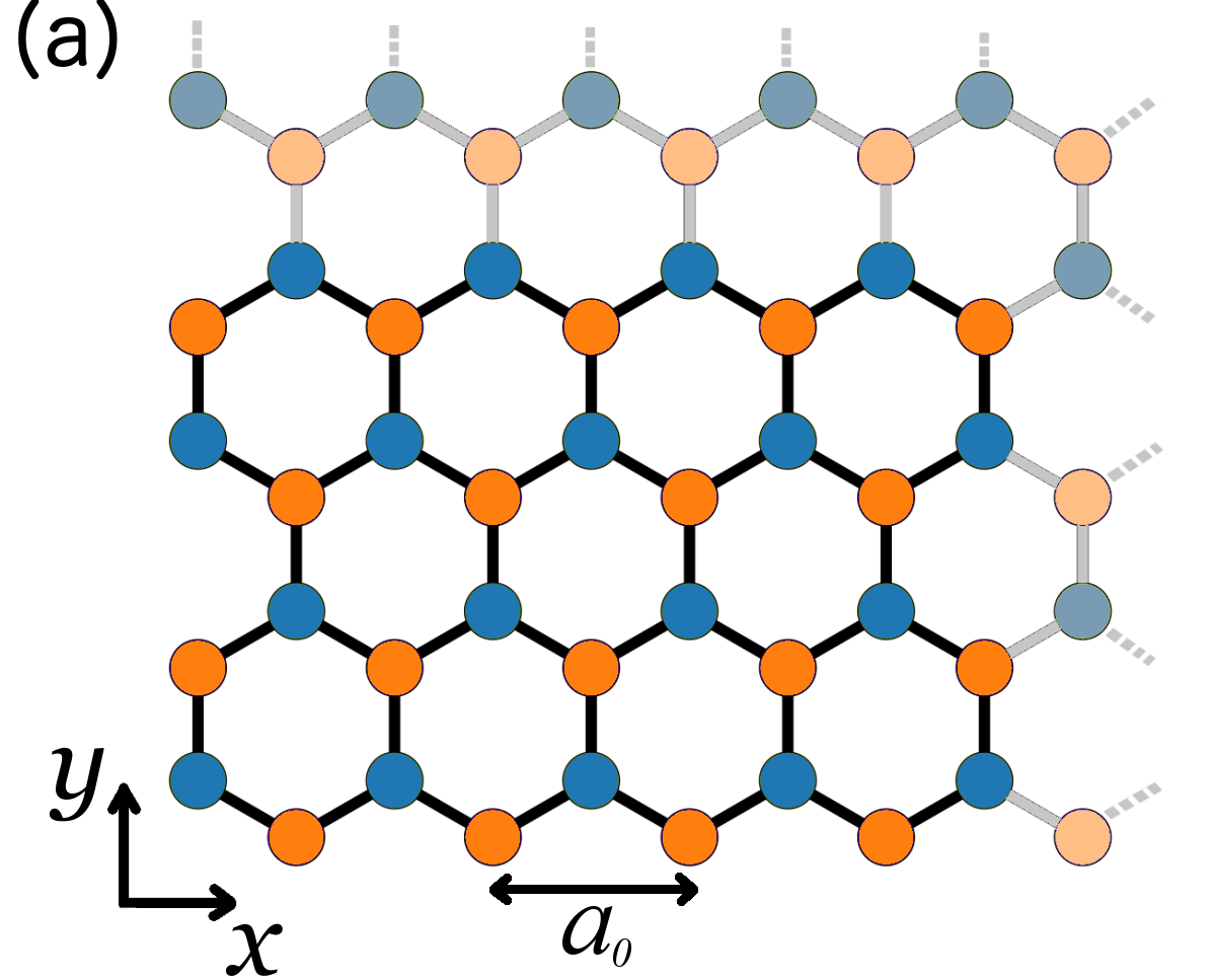
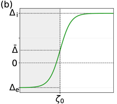
Figure 1: (a) Sketch of the system with $x$ and $y$ directions. In the analytical calculation the system is a semi-infinte half plane. In the numerical calculations it has a ribbon geometry, attached to source and drain leads. Depending on the orientation, it is a system with either zigzag, or armchair edges. (b) Sketch of the profile of the space modulation of the intrinsic SOC given by Eq. (3). The system occupies the unshaded region.

Within the LWA approximation, graphene’s effective Hamiltonian is given by

$$\mathcal{H}=v_{F}(\tau_{z}\sigma_{x}\hat{p}_{x}+\sigma_{y}\hat{p}_{y})+\Delta\tau_{z}\sigma_{z}s_{z}\,,$$ (1)

where $v_{F}$ denotes graphene’s Fermi velocity, $\bm{p}=-i\hbar\bm{\nabla}$ is the momentum operator, and $\{\tau_{x},\tau_{y},\tau_{z}\}$/$\{\sigma_{x},\sigma_{y},\sigma_{z}\}$/$\{s_{x},s_{y},s_{z}\}$ are the Pauli matrices associated to the valley/sublattice/spin degree of freedom, respectively. Since the Hamiltonian (1) is diagonal in valley and spin space, we will work in a basis of given valley and spin projection:

$$\Psi_{\tau,s}=\begin{pmatrix}v_{A,\tau,s}\\ v_{B,\tau,s}\end{pmatrix},\quad\tau,s=\pm 1,$$ (2)

and we shall omit the valley and spin indices wherever there is no risk of confusion. In Eq. (1), we include a non-uniform intrinsic SOC with a smooth spatial modulation transverse to the boundary:

$$\Delta(\zeta) =\bar{\Delta}+\Delta_{0}\tanh\left(\frac{\zeta-\zeta_{0}}{\ell}\right).$$ (3)

Here, $\zeta$ represents the coordinate in the direction perpendicular to the boundary, located at $\zeta=0$, and the system extends on the side of positive $\zeta$. Equation (3) describes a domain-wall profile centered at $\zeta=\zeta_{0}$, with characteristic modulation length $\ell$, and with asymptotic values given by

$$\Delta_{\text{i,e}} =\bar{\Delta}\pm\Delta_{0}.$$ (4)

Then $\Delta_{\text{i}}$ represents the SOC deep in the interior of the nanoribbon. We assume that the modulation occurs close to the boundary, where the SOC reduces to $\bar{\Delta}$, with $\zeta_{0}$ of the order of graphene’s lattice constant $a_{0}$, see Fig. 1(b).

The choice of the hyperbolic tangent profile is convenient because it allows for an exact solution of the corresponding Dirac equation Landau and Lifshitz (1986); Tchoumakov et al. (2017). However, we expect that the qualitative features of the spectrum do not depend on the detailed shape of the profile, as long as the typical length scale $\ell$ of the SOC modulation is large on the scale of the lattice constant $a_{0}$. Since this is also the condition for the validity of the LWA employed here, throughout this paper we assume $\ell\gg a_{0}$.

II.1 Spectral properties of zigzag ribbons

We start by considering a semi-infinite graphene flake extending in the region $y>0$, with a zigzag edge along the $x$-axis [see Fig. 1(a)], and SOC profile given by Eq. (3) with $\zeta=y$. By exploiting the translational invariance along the $x$-direction, the wave function can be expressed in the form

$$\Psi(x,y)=e^{ik_{x}x}\psi(y),$$ (5)

with $\psi^{T}(y)=(v_{A},v_{B})$. Then, the Dirac equation reduces to

$$\left[\tau\sigma_{x}k_{x}-i\sigma_{y}\partial_{y}+s\tau\Delta(y)\sigma_{z}\right]\psi=E\psi\,,$$ (6)

where we set $\hbar=1$, and measure energies in units of $v_{F}/\ell$, lengths in units of $\ell$, and wave vectors in units of $\ell^{-1}$. Equation (6) admits an exact solution Landau and Lifshitz (1986); Tchoumakov et al. (2017), whose derivation is summarized in App. A. Here, we just present the result. We introduce the notation

$$\kappa_{\text{i/e}}=\sqrt{k^{2}_{x}+\Delta_{\text{i/e}}^{2}-E^{2}}\,,\qquad\bar{\kappa}=\frac{\kappa_{\text{i}}+\kappa_{\text{e}}}{2}\,.$$ (7)

Then, in terms of the new variable $u$ given by

$$u=\frac{1}{2}\left[1-\tanh(y-y_{0})\right],$$

the sublattice amplitudes can be expressed as

$$v_{\alpha}=u^{\kappa_{\text{i}}/2}(1-u)^{\kappa_{\text{e}}/2}(w_{+}+\alpha\,w_{-})\,,$$ (8)

with $\alpha=A,B=\pm$. The functions $w_{\pm}(u)$ satisfy a hypergeometric equation (see App. A). Selecting the solution that leads to normalizable states for $y\rightarrow+\infty$ (i.e., $u\rightarrow 0$), we obtain

$$w_{\pm}(u) =c_{\pm}\,F[\bar{\kappa}\pm s\tau\Delta_{0},\bar{\kappa}\mp s\tau\Delta_{0}+1;\kappa_{\text{i}}+1;u],$$ (9)

where $F(a,b;c;z)$ is the ordinary hypergeometric function Olver et al. (2010). Normalizability requires $\kappa_{\text{i}}>0$, but imposes no constraint on $\kappa_{\text{e}}$. Therefore, at fixed $k_{x}$, the edge modes exist in energy window $|E|<\sqrt{\Delta^{2}_{\text{i}}+k_{x}^{2}}$. Since for $y\rightarrow+\infty$ we have $u\sim e^{-2y}$, $\kappa^{-1}_{\text{i}}$ actually represents the decay length of the corresponding edge mode into the bulk. The relative factor between the two spinor components is fixed by the Dirac equation. We find

$$\frac{c_{-}}{c_{+}}=\frac{\kappa_{\text{i}}+s\tau\Delta_{\text{i}}}{E+\tau k_{x}}\,.$$ (10)

We now need to impose the appropriate boundary condition. In the case of a zigzag edge, the boundary condition requires that one sublattice component of the wave function vanishes at the boundary $y=0$, separately for each valley and spin Brey and Fertig (2006); Castro Neto et al. (2009):

$$v_{\alpha,\tau,s}(0)=0,\quad\tau,s=\pm 1\,,$$ (11)

where $\alpha=A$ (respectively $\alpha=B$) if the boundary sites belong to the $B$ (respectively $A$) sublattice. Using Eqs. (8), (9), and (10), from Eq. (11) we obtain

$$\frac{(E+\tau k_{x})F[\bar{\kappa}+s\tau\Delta_{0},\bar{\kappa}-s\tau\Delta_{0}+1;\kappa_{\text{i}}+1;u_{0}]}{(\kappa_{\text{i}}+s\tau\Delta_{\text{i}})F[\bar{\kappa}-s\tau\Delta_{0},\bar{\kappa}+s\tau\Delta_{0}+1;\kappa_{\text{i}}+1;u_{0}]}\!=\!-\alpha,$$ (12)

where $u_{0}=\frac{1}{2}(1+\tanh y_{0})$. The shift $y_{0}$ is important for the comparison to the numerical tight-binding analysis, in which the SOC profile is centered exactly at the edge of the system, i.e., on the first line of carbon atoms Wakabayashi et al. (2010). In the continuum approach, this corresponds to the choice $y_{0}=a_{0}/\sqrt{3}$, because $y=0$ corresponds to a line of auxiliary sites, where one imposes the vanishing of the wave function.

Before discussing the solutions of Eq. (12), we notice that this equation is invariant under the following transformations:

$$\tau,s,k_{x}\rightarrow-\tau,-s,-k_{x}\,,$$

$$E,k_{x},\alpha\rightarrow-E,-k_{x},-\alpha\,.$$

The first invariance is just the consequence of the time-reversal symmetry of the Hamiltonian (1): the edge states occur in pairs of counterpropagating modes with opposite spins, residing on opposite valleys. The second invariance implies that the edge state spectrum at a $B$-type edge can be obtained from the spectrum at an $A$-type edge by simply reversing energy and wave vector. In order to reproduce the full spectrum of edge states (including degeneracies) of a wide zigzag nanoribbon, which has one edge of $A$ sites and one edge of $B$ sites, we need to take the solutions of Eq. (12) with $\alpha=+1$ and with $\alpha=-1$. These solutions are shown in Fig. 2 as blue dots on top of the numerical results discussed in the next sections (gray, black, and red lines). For clarity, we only include the states at one valley, the states at the other valley follow by symmetry.

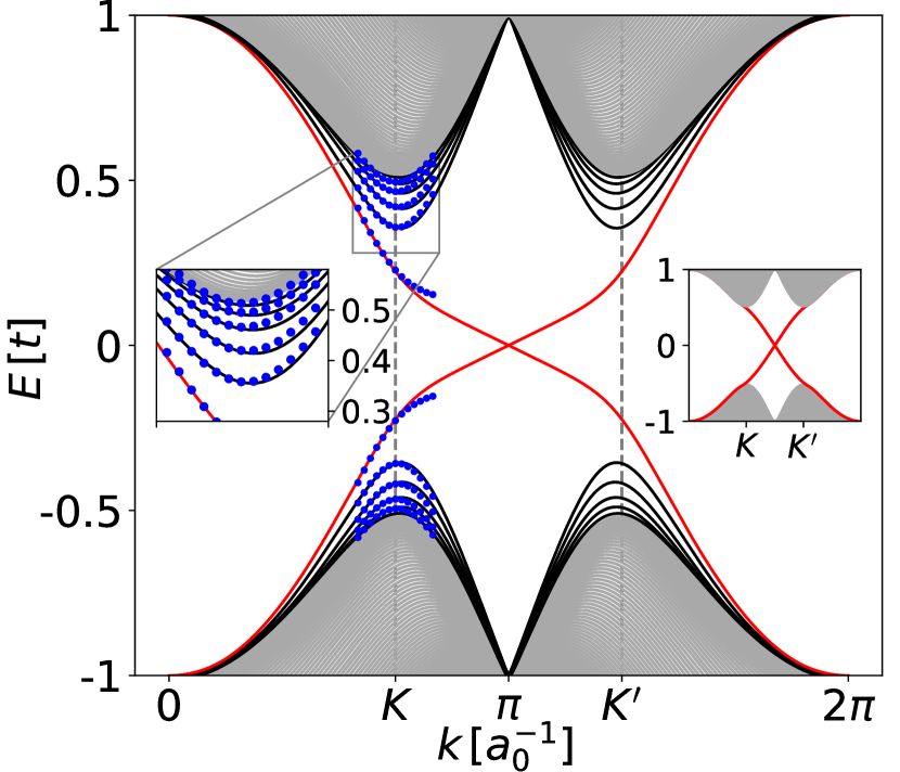
Figure 2: Band structure of a zigzag nanoribbon of width $L_{y}=37.2$ nm ($150$ rows), with modulation of the SOC at the boundary. We set $\lambda_{\text{i}}=0.1t$, $\lambda_{\text{e}}=-0.05t$, and $\ell=12a_{0}$. The gray, black, and red lines are the tight-binding results, describing bulk states, VP states, and topological states, respectively. The analytical results from Eq. (12) are represented as blue dots. The right inset shows the case of homogeneous SOC, with $\lambda=0.1t$, corresponding to a gap $\Delta=3\sqrt{3}\lambda\approx 0.52t$. In both cases, two topological modes (red lines) cross within the gap. The modulation of the SOC results in additional massive edge states, popping up under the conduction band and above the valence band (black lines).

We observe that the continuum approach faithfully reproduces all the main features of the spectrum close to the Dirac points. Within the gap, there exist two topological bands with approximately linear dispersion, and ten massive VP modes (for the given values of the parameters), in agreement with the results of the numerical approach discussed in Sec. III below. All these levels are doubly degenerate if one considers a system with two edges. Figure 2 shows the agreement between analytical and numerical results. For wave vectors in the interval between the two Dirac points, the agreement is less satisfactory, which we attribute to the fact that the coupling between the valleys, neglected in the continuum approach, plays an important role at these wave vectors. This is especially evident for the topological bands. Another source of discrepancy stems from neglecting higher order terms in momentum in the LWA.

II.2 Spectral properties of armchair ribbons

Let us now turn to the case of a semi-infinite system with an armchair edge along the $y$-direction [see Fig. 1(b)]. The wave function can be written as

$$\Psi(x,y)=e^{ik_{y}y}\psi(x)\,,$$ (13)

with $\psi^{T}(x)=(v_{A},v_{B})$. Then the Dirac equation reduces to

$$\left[-i\tau\sigma_{x}\partial_{x}+\sigma_{y}k_{y}+s\tau\Delta(y)\sigma_{z}\right]\psi=E\psi\,,$$ (14)

and its solutions can be written as

$$v_{A} =u^{\kappa_{\text{i}}/2}(1-u)^{\kappa_{\text{e}}/2}(\tilde{w}_{+}+\tilde{w}_{-})\,,$$ (15a)

$$v_{B} =iu^{\kappa_{\text{i}}/2}(1-u)^{\kappa_{\text{e}}/2}(\tilde{w}_{+}-\tilde{w}_{-})\,,$$ (15b)

where $u=\frac{1}{2}[1-\tanh(x-x_{0})]$. The functions $\tilde{w}_{\pm}$ are, again, solutions of a hypergeometric equation, and are given by

$$\tilde{w}_{\pm}(u) =d_{\pm}\,F[\bar{\kappa}\mp s\Delta_{0},\bar{\kappa}\pm s\Delta_{0}+1;\kappa_{\text{i}}+1;u],$$ (16)

with the relative factor, fixed by the Dirac equation, given by

$$\frac{d_{-}}{d_{+}}=\frac{\tau(s\Delta_{\text{i}}-\kappa_{\text{i}})}{E+k_{y}}\,.$$ (17)

Notice that the dependence on the valley index only appears in the prefactor.

In the armchair case, the boundary condition involves both valleys Brey and Fertig (2006); Castro Neto et al. (2009) and reads

$$\left[v_{\alpha,\tau=+1,s}+v_{\alpha,\tau=-1,s}\right]_{x=0}=0\,,\quad s=\pm 1\,,$$ (18)

with $\alpha=A,B$. In terms of the $w_{\pm}$ we find

$$\left[\tilde{w}_{\pm,\tau=+1}+\tilde{w}_{\pm,\tau=-1}\right]_{u=u_{0}}=0\,,\quad s=\pm 1\,.$$ (19)

From Eq. (17) we see that either $\tilde{w}_{-,\tau=-1}=-\tilde{w}_{-,\tau=1}$ or $\tilde{w}_{+,\tau=-1}=-\tilde{w}_{+,\tau=1}$, therefore the boundary condition takes the simple form

$$(E\pm k_{y})F[\bar{\kappa}\mp s\Delta_{0},\bar{\kappa}\pm s\Delta_{0}+1;\kappa_{\text{i}}+1;u_{0}]=0\,.$$ (20)

Here, $u_{0}=\frac{1}{2}(1+\tanh x_{0})$. In the armchair system, the shift required to have the correct value of the SOC on the first line of carbon atoms is $x_{0}=a_{0}/2$.

The solutions to Eq. (20) are shown in Fig. 3 as blue dots. As in the zigzag case, in a nanoribbon all levels are doubly degenerate, corresponding to states on both edges. The obvious solutions $E=\mp k_{y}$ describe two counterpropagating linearly dispersing topological bands. These modes only exist if $s=\mp 1$, respectively, otherwise one gets the trivial solution $\tilde{w}_{+}=\tilde{w}_{-}=0$. The allowed value of $s$ guarantees that the corresponding wave function is normalizable. This is a manifestation of the spin-momentum locking. Remarkably, in contrast to the zigzag case, here the group velocity of the topological modes is equal to $v_{F}$ and does not depend on SOC. Moreover, we observe that, for $E\neq\pm k_{y}$, the boundary condition depends on $k_{y}$ and $E$ only through the combination $k_{y}^{2}-E^{2}$. Therefore we find solutions corresponding to VP states, whose dispersion has the form

$$E_{n}=\pm\sqrt{M^{2}_{n}+k^{2}_{y}}\,,\quad n=1,\dots,N_{\text{max}}\,,$$ (21)

where the effective masses $M_{n}$ and the number of massive states $N_{\text{max}}$ depend on the parameter values. In Fig. 3, we compare the analytical results with the numerical ones, finding an excellent agreement. Since in this case the continuum approach incorporates the coupling between valleys in the boundary condition, it is not surprising that the agreement is better than in the zigzag case.

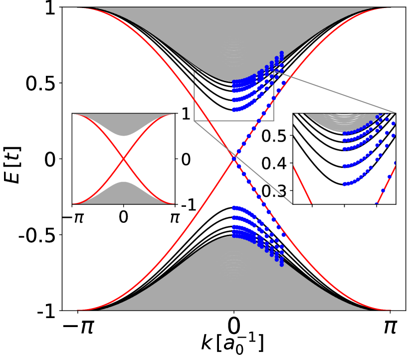
Figure 3: Band structure for an armchair nanoribbon of width $L_{x}=32.5$ nm ($128$ rows), with SOC modulation near the boundary. We set $\lambda_{\text{i}}=0.1t$, $\lambda_{\text{e}}=-0.05t$, and $\ell=12a_{0}$. The gray, black, and red lines are the tight-binding results, describing respectively bulk states, VP states, and topological states. The blue dots are the solutions of Eq. (20). Close to the $\mathbf{K}$ ($\mathbf{K^{\prime}}$) point (in the armchair case, projected to $k=0$), the agreement is excellent. The right inset shows the case of homogeneous SOC with $\lambda=0.1t$, corresponding to a gap $\Delta=3\sqrt{3}\lambda\approx 0.52t$.

III Numerical tight-binding model

In order to be able to go beyond the low-energy approximation, as well as to study the transport properties, we now move on to a fully numerical approach within a tight-binding formalism, which we implement using Kwant Groth et al. (2014). Contrary to the analytical calculation, we will here consider a finite size system, comprising of a scattering region with two edges, along which edge states can propagate, and a source and a drain lead, which are seamlessly coupled to the scattering region. We will take rather large ribbons, but still of experimentally relevant sizes, with length $L\approx 60$ nm and width $W\approx 35$ nm. For this width, which largely exceeds the modulation length $\ell=12\,a_{0}\approx 3$ nm, the electronic states located on opposite edges do not overlap. Hence, the edges are independent, and the numerical results can readily be compared to the analytical solution for a semi-infinite system. For the local

III.1 The model and its parameters

Within a tight-binding formalism, the Hamiltonian for graphene with intrinsic SOC reads Kane and Mele (2005a, b):

$$\mathcal{H}=-t\!\!\sum_{\begin{subarray}{c}\langle n,m\rangle\\ s\end{subarray}}c_{ns}^{\dagger}c_{ms}+i\lambda\!\!\!\!\!\sum_{\begin{subarray}{c}\langle\langle n,m\rangle\rangle\\ ss^{\prime}\end{subarray}}\nu_{nm}(s_{z})_{ss^{\prime}}c_{ns}^{\dagger}c_{ms^{\prime}}\,,$$ (22)

where $c_{ns}^{\dagger}$ ($c_{ns}$) creates (annihilates) an electron with spin $s$ on the site $n$, and the symbol $\langle\ldots\rangle$ ($\langle\langle\ldots\rangle\rangle$) indicates sum over nearest (next nearest) neighbour sites. In Eq. (22), the sign $\nu_{nm}=\pm 1$ depends on the orientation of the next nearest neighbour hopping: it is positive (negative) for electron making a left (right) turn to the next nearest neighbour carbon atom. The hopping parameter is $t$, and $\lambda$ is the intrinsic SOC parameter, which is related to the gap size as $\Delta=3\sqrt{3}\lambda$.

We consider the following space modulation of the intrinsic SOC along the coordinate corresponding to the lateral width of the graphene nanoribbon:

$$\lambda(\zeta) =\frac{\lambda_{\text{i}}+\lambda_{\text{e}}}{2}$$ (23)

$$+\frac{\lambda_{\text{i}}-\lambda_{\text{e}}}{2}\Big{[}\tanh\left(\frac{\zeta}{\ell}\right)-\tanh\left(\frac{\zeta-L_{\zeta}}{\ell}\right)-1\Big{]}\,,$$

where $L_{\zeta}$ is the width of the ribbon in the $\zeta$-direction, and $\lambda_{\text{i(e)}}$ is the value of the SOC in the internal (external) region of the ribbon, respectively. Throughout this paper, we use $\lambda_{\text{i}}=0.1t$ and $\lambda_{\text{e}}=-0.05t$. The length scale $\ell$ characterizes the size of the spatial region over which the variation of the intrinsic SOC takes place. This has to be compared with the three natural length scales present in the system: the lattice constant $a_{0}$, the length scale associated to the SOC gap $\xi=\hbar v_{\text{F}}/\Delta$, and the width of the ribbon $L_{\zeta}$. In order to get VP states, one has to assure $\ell\gtrsim\xi$. Moreover, to resolve the smoothness of the SOC modulation one needs $\ell\gg a_{0}$, and the two edges are independent for $L_{\zeta}\gg\ell$. In App. B we provide some details on the relation between the parameter values in the LWA and in the tight-binding model.

III.2 Spectral properties

In this section we investigate the spectral properties of graphene nanoribbons: the band structure and the local density of states (LDOS). The band structure for homogeneous SOC are shown in the insets of Figs. 2 and 3. Without SOC modulation, each edge of the system hosts two topological states with linear dispersion, as shown in the insets in red. The bulk states, in gray, form the conductance band (CB) and the valence band (VB).

For the calculation of the LDOS, Kwant first calculates the available modes in the semi-infinite source lead. These modes are then projected onto the scattering matrix of the scattering region.

III.2.1 Zigzag ribbons

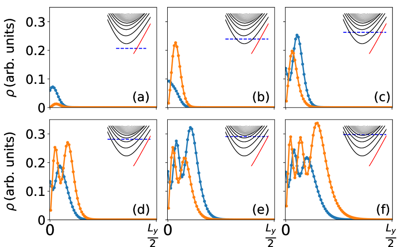
Figure 4: Local density of states at one edge of a zigzag nanoribbon, for $A$ (orange) and $B$ (blue) sublattices, summed over the spin. On the opposite edge, $A$ and $B$ sublattices should be exchanged. In the inset, the energy at which the LDOS is evaluated is indicated by the dashed-blue line in the band structure.

In the zigzag case, we consider a ribbon of width $W=L_{y}=37.2$ nm, corresponding to $150$ rows. Figure 2 shows that, due to the suppression of the SOC near the edges, VP bands are pulled out of the CB and the VB, in symmetric fashion. Near the $\mathbf{K}$ and $\mathbf{K}^{\prime}$ points, these VP modes push away the topological modes, whose group velocity is thus strongly affected. This feature can be rationalized by observing that, from Eq. (12), one can see that the group velocity of the topological modes close to the Dirac points depends strongly on the gap parameters $\Delta_{\text{i/e}}$.

Near the boundary, as the SOC gets weaker, the effective gap becomes smaller. Looking at the VP modes under the CB, we observe that the first (lowest in energy) VP mode is the one which lies closest to the edge, and has the smallest decay length. Each consecutive VP mode has a longer decay length and extends deeper in the bulk, and therefore “sees” a slightly larger effective gap.

In Fig. 4 the LDOS of the edge states is plotted at different energies. In Fig. 4(a) there is only the topological mode, in 4(b) there is additionally one VP mode, in 4(c) two VP modes etc. In the zigzag case we observe that there are zones on the lattice with predominant $A$ or $B$ contributions to the LDOS. Moreover, for each VP mode that is added, the predominance changes sublattice.

III.2.2 Armchair ribbons

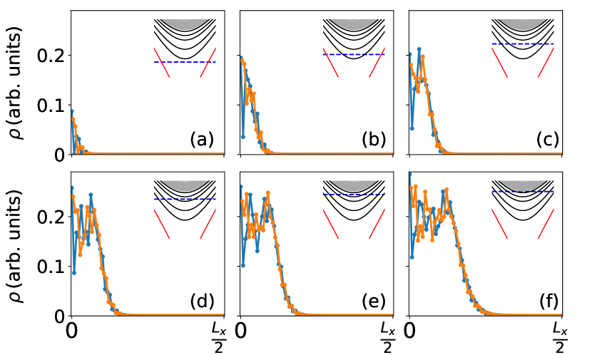
Figure 5: Local density of states at one edge of an armchair nanoribbon, for A (orange) and B (blue) sublattice, summed over the spin, with the corresponding energy indicated in the inset as a dashed-blue line in the band structure.

In the armchair case, we consider a ribbon of width $W=L_{x}=32.5$ nm, corresponding to $128$ unit cells. The band structure is shown in Fig. 3. The two Dirac points are projected onto the same point $k=0$. In the absence of SOC, an armchair ribbon is metallic or semiconducting, depending on its exact width Castro Neto et al. (2009). In the case studied here, the ribbon is wide enough that the semiconducting gap, which is of order of $\hbar v_{F}/L_{x}$, is exceedingly small compared to all other energy scales, and can be ignored. In the presence of SOC, the gap size is then determined by the SOC strength, and there are always two topological modes crossing the gap. With the SOC modulation, new massive bands appear under the CB and above the VB. However, in contrast to the zigzag case, the dispersion of the topological bands is not affected by the appearance of these new levels, and their group velocity is not modified. This is consistent with the analytical solution of Eq. (20), which gives a linear dispersion with slope $v_{F}$, independent of the values of the gap parameters. As shown in Fig. 3, the agreement between the analytical and numerical results for all edge states is excellent.

In the LDOS for an armchair ribbon we see there are no privileged $A$ or $B$ sublattice zones — Fig. 5. It is harder in this case to say where on the lattice the different VP states lie. Also in this case, we observe the expansion of the area containing the edge states, as one consecutively adds subbands.

IV Transport properties

In this section we will investigate if two-terminal conductance measurements on nanoribbons with SOC modulation near the edges could reveal the presence of VP states. Being massive, VP states are not protected against backscattering due to disorder. We will therefore add Anderson disorder to the model, namely random spin-independent onsite energies with uniform probability distribution in the interval $\varepsilon_{n}\in[-U_{0}/2,\,U_{0}/2]$. The disorder Hamiltonian can be written as

$$H_{\text{D}}=\sum_{ns}\varepsilon_{n}c_{ns}^{\dagger}c_{ns}\,,$$ (24)

where the sum runs over the entire system. The topological edge states will not be sensitive to this disorder, but the VP states will. How much the disorder weakens the VP states depends not only on the disorder strength, but also on the system size. Here, we consider a sample of size $L\times W\approx 60\times 35$ nm².

IV.1 In-gap conductance

The numerical results for the two-terminal conductance are shown in Fig. 6. As one can expect for a system presenting in-gap states, the conductance never decreases to zero. Here, we have two counterpropagating doubly-degenerate topological edge states in the gap, so the minimal in-gap conductance is $2e^{2}/h$. In the absence of SOC modulation, this is the only in-gap contribution to the conductance. With SOC modulation near the edges, we observe clear steps at the energies at which new VP modes open, see upper panels of Fig. 6. Both in the zigzag as well as in the armchair cases, these steps are symmetric around the gap center $E=0$.

In the presence of disorder, the conductance due to the VP modes is suppressed, because those modes are sensitive to backscattering. For strong disorder, the conductance reduces to $2e^{2}/h$, below which it can not descend because the topological modes are not sensitive to Anderson disorder, which does not break time-reversal symmetry. However, in this case the conductance in the CB and the VB is also significantly reduced due to the disorder in the ribbon. Remarkably, within a certain range of disorder strength, we observe dips in the conductance at the step edges. This reminds of the physics of a quasi-1D quantum wire containing an impurity with an attractive potential, where the conducting modes couple to a quasi-bound state at the impurity Bagwell (1990).

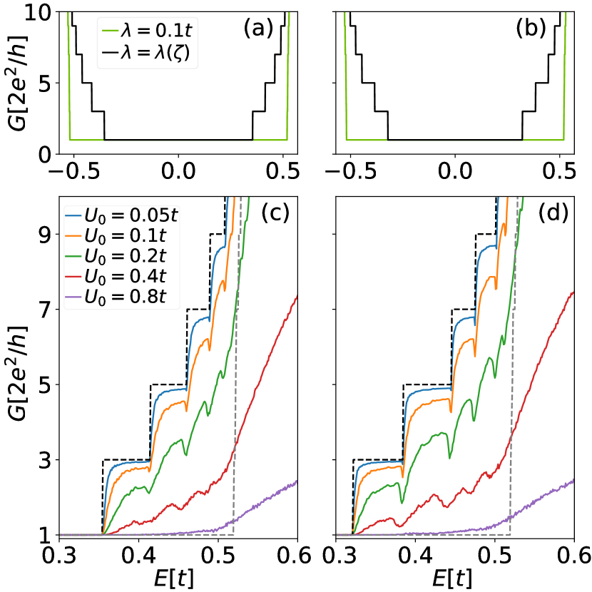
Figure 6: Conductance for a clean ribbon without (grey) and with (black) modulation of the SOC interaction for a zigzag (a) and armchair (b) ribbon. In the case with modulation $\lambda_{\text{i}}=0.1t$ and $\lambda_{\text{e}}=-0.05t$. The lower panels (c)-(d) are a zoom around the CB edge, where the VP modes are, for several disorder strengths. Within the range $U_{0}\in[0.05,0.4]$ clear conductance minima are observed just before the opening of a new VP mode.

IV.2 Dip behavior near the steps

In the lower panels of Fig. 6, we observe a minimum at each step in the conductance curve of the disordered system. Notice that each line represents the conductance averaged over 100 disorder configurations. Plotting single disorder configurations [c.f. App. C], one observes random fluctuations at the plateaus, which average out over many disorder configurations, as well as a dip at the step edges, which most configurations have in common, and which therefore remains in the averaged conductance. Such dips in the conductance at the opening of new subbands were discussed in detail in a paper by Bagwell Bagwell (1990); Tekman and Bagwell (1993), in which he shows how propagating modes in a narrow wire with parabolic confinement couple to the zero energy quasi-bound states of delta shaped, negative potential impurities. Similar dips were also explored in the context of quantum Hall states Palacios and Tejedor (1993); Haug (1993). In the case presented here, in the energy gap we have to deal with a quasi-1D subsystem near the edge, with triangular confinement potential. The quasi-bound states can be hosted in local energy minima, that appear due to the random energy landscape. In order to verify that we are indeed dealing with this physical phenomenon, we have simulated a clean sample, containing one Gaussian-shaped impurity at each edge. We investigated the minimal requirements for observing dips in the conductance curves right at the onset of the steps. The simulations with single impurities clearly demonstrate that the dips come from the coupling of the propagating states to quasi-bound states lying at randomly distributed energy minima on the lattice. This can be observed in strongly confined quasi-1D systems with an attractive impurity (negative potential). The precise properties of the dip in the conductance depend on the shape and strength of the impurity, and other system details. Additional information is given in App. C.

Although the situation near the edges in the system presented here differs from that investigated in earlier works, many of the physical arguments still hold Chu and Sorbello (1989); Bagwell (1990). Because of the random energy landscape, attractive sites or regions on the lattice may result in the appearance of quasi-bound states lying just under each VP subband. As we can observe, and as is normally the case, the evanescent state under the lowest VP subband is a true bound state, as it does not couple to the topological state. We therefore observe no dip before the first step, i.e. conductance never decreases below $2e^{2}/h$. We also observe the usual renormalization of the energy gap, which slightly shifts the energies of the onsets of the steps, and the value of the CB opening Groth et al. (2009); Jiang et al. (2009); Wu et al. (2016). The binding energy, defined as the difference in energy between the step edge and the dip minimum, is therefore hard to quantify. However, we do observe that, as disorder gets stronger, the dips become deeper, which is in line with earlier observations. In wires with a parabolic confinement potential and single attractive impurities, the interaction strength between the impurity and the various available subbands depends on the lateral position of the impurity in the wire. For our triangular confinement near the edge there is no symmetry around any center, however, we know where at the edge each of the modes lies, and if it can interact with the impurity. In the implementation of our system with one single impurity at each edge, we clearly observe how the impurity interacts with consecutive edge states as we move it away from the edge towards the bulk of the sample, as discussed above. A more in depth investigation is beyond the scope of this work, but will be the subject of a future investigation.

V Conclusion and outlook

In this work, we have investigated the appearance of Volkov-Pankratov edge states in topological graphene nanoribbons of zigzag and armchair type. In the presence of intrinsic SOC which is smoothly suppressed near the edges, the well-known QSH edge states are accompanied by multiple massive VP states. We have demonstrated their existence by means of two complementary methods, the exact analytical solution of the low-energy effective Dirac equation, and the numerical tight-binding approach, finding good agreement between the two.

Transport simulations show how the VP modes contribute to transport, also in the presence of disorder. We observe dips in the conductance at the onset of each VP band, which are due to the coupling of the propagating VP states to evanescent modes present in the random energy landscape. At sufficiently strong disorder, the VP states are entirely suppressed, and cease to contribute to transport.

Our results can be relevant to experimental systems in which the intrinsic SOC in graphene is enhanced by one of the methods mentioned in the Introduction. Both the deposition of adatoms, as well as the proximitization with a TMD layer, would likely give rise to a inhomogeneous intrinsic SOC, especially at the edges of the system.

In addition to a possible implementation in graphene or “post-graphene” materials, the presence of these VP states accompanying the topological modes could be achieved in systems of ultracold atoms in optical lattices. The advantage of a realization within this platform is related to the flexibility to control the parameters separately across a large range compared to condensed-matter systems, where the system parameters are generally fixed by the material properties and by the sample geometry Bloch et al. (2008).

The time-reversal symmetric Kane-Mele model for the QSH effect Kane and Mele (2005b, a) can be thought of as a double copy of the Haldane model Haldane (1988) in which time-reversal symmetry is broken. The implementation of the Kane-Mele model could be achieved within the state-of-the-art technology for ultracold atoms; the honeycomb lattice and the Haldane model have been already realized in this context Tarruell et al. (2012); Jotzu et al. (2014). In practice, the Kane-Mele model could be implemented by using an internal atomic state as a spin degree of freedom. For each spin, the same scheme as for the Haldane model could be used to implement the second-next-neighbour hopping, see Ref. Goldman et al. (2010); Bercioux et al. (2011); Goldman et al. (2011). This system would then correspond to two copies of the Haldane model Jotzu et al. (2014). Contrary to the implementation in Ref. Goldman et al. (2016), we propose to realize a system with a homogeneous intrinsic SOC and soft-boundary conditions, corresponding to an inhomogeneous onsite energy profile due to the confining potential of the atomic trap. Similar to the results presented in this work, this scheme gives rise to a set of VP states accompanying the topologically protected one, but with energy symmetry breaking. A similar approach was proposed for the case of the quantum Hall edge states Buchhold et al. (2012). Other aspects of the implementation of this model for ultracold atoms require further investigation.

Appendix A Solution of the Dirac equation with inhomogeneous SOC

In order to make this paper self-consistent, in this appendix we provide the details of the exact solution of the Dirac equation in the presence of an inhomogeneous SOC with hyperbolic tangent profile. The analysis follows Refs. Tchoumakov et al. (2017); Landau and Lifshitz (1986).

A.1 Zigzag case

We consider first the case of a semi-infinite system with a zigzag edge along the $x$-direction, see Fig. 1(a). After factorization of a plane wave in the $x$-direction with wave vector $k_{x}$, the Dirac equation reads

$$\left\{\tau\sigma_{x}k_{x}-i\sigma_{y}\frac{d}{dy}+\sigma_{z}s\tau\left[\bar{\Delta}+\Delta_{0}\tanh(y-y_{0})\right]\right\}\psi(y)=E\psi(y)\,,$$ (25)

where we set $\hbar=1$, and measure energies in units of $v_{F}/\ell$, lengths in units of $\ell$, and wave vectors in units of $\ell^{-1}$. We look for solution on the half-line $y\geq 0$. Squaring Eq. (25), we obtain

$$\left[\frac{d^{2}}{dy^{2}}+(E^{2}-k^{2}_{x}-\bar{\Delta}^{2}-\Delta^{2}_{0})+\frac{\Delta_{0}(\Delta_{0}-s\tau\sigma_{x})}{\cosh^{2}(y-y_{0})}-2\bar{\Delta}\Delta_{0}\tanh(y-y_{0})\right]\psi(y)=0\,.$$ (26)

Next, we express $\psi$ as

$$\psi=\left(\begin{array}[]{c}v_{A}\\ v_{B}\end{array}\right)=\phi_{+}|+\rangle+\phi_{-}|-\rangle,\qquad v_{A/B}=\frac{1}{\sqrt{2}}\left(\phi_{+}\pm\phi_{-}\right)\,,$$

where $|\pm\rangle$ are the eigenvectors of $\sigma_{x}$, with respective eigenvalue $\pm 1$. By performing the change of variable

$$u=\frac{1}{2}\left[1-\tanh(y-y_{0})\right]\,,$$

Eq. (27) can be rewritten as

$$\left[u(1-u)\frac{d}{du}u(1-u)\frac{d}{du}-\frac{1}{4}(\kappa_{\text{i}}^{2}(1-u)+\kappa_{\text{e}}^{2}u)+(\Delta^{2}_{0}-rs\tau\Delta_{0})u(1-u)\right]\phi_{r}=0,\quad r=\pm\,,$$ (27)

where we use the notation

$$\kappa_{\text{i/e}}=\sqrt{k_{x}^{2}+\Delta^{2}_{\text{i/e}}-E^{2}}\,,\quad\bar{\kappa}=\frac{\kappa_{\text{i}}+\kappa_{\text{e}}}{2}\,.$$

Substituting in Eq. (27) the ansatz

$$\phi_{r}(u)=u^{\kappa_{\text{i}}/2}(1-u)^{\kappa_{\text{e}}/2}w_{r}(u)\,,$$

we find the hypergeometric equation

$$u(1-u)w^{\prime\prime}_{r}+\left[(\kappa_{\text{i}}+1)-(2\bar{\kappa}+2)u\right]w^{\prime}_{r}-\left[\left(\bar{\kappa}+rs\tau\Delta_{0}\right)\left(\bar{\kappa}-rs\tau\Delta_{0}+1\right)\right]w_{r}=0\,.$$ (28)

We need to select the solution which leads to normalizable states for $y\rightarrow+\infty$, i.e., $u\rightarrow 0$. We find

$$w_{+}(u) =c_{+}\,F[\bar{\kappa}+s\tau\Delta_{0},\bar{\kappa}-s\tau\Delta_{0}+1;\kappa_{\text{i}}+1;u]\,,$$ (29a)

$$w_{-}(u) =c_{-}\,F[\bar{\kappa}-s\tau\Delta_{0},\bar{\kappa}+s\tau\Delta_{0}+1;\kappa_{\text{i}}+1;u]\,,$$ (29b)

where $F[a,b;c;z]$ is the ordinary hypergeometric function Olver et al. (2010). Notice that $F[a,b;c;z]=F[b,a;c;z]$. The other solution to the hypergeometric equation does not lead to normalizable states and we omit it. Since we consider a semi-infinite system, in contrast to Ref. Tchoumakov et al. (2017), we do not require normalizability for $y\rightarrow-\infty$, but we need to impose the appropriate boundary condition at $y=0$, as discussed in the main text. The relative factor between the two components is fixed by the Dirac equation, and we find

$$\frac{c_{-}}{c_{+}}=\frac{\kappa_{\text{i}}+s\tau\Delta_{\text{i}}}{\tau k_{x}+E}=\frac{\tau k_{x}-E}{\kappa_{\text{i}}-s\tau\Delta_{\text{i}}}\,.$$

Then, to summarize, up to an overall normalization factor, we have

$$\phi_{+} =(\tau k_{x}+E)u^{\kappa_{\text{i}}/2}(1-u)^{\kappa_{\text{e}}/2}F[\bar{\kappa}+s\tau\Delta_{0},\bar{\kappa}-s\tau\Delta_{0}+1;\kappa_{\text{i}}+1;u]\,,$$ (30a)

$$\phi_{-} =(\kappa_{\text{i}}+s\tau\Delta_{\text{i}})u^{\kappa_{\text{i}}/2}(1-u)^{\kappa_{\text{e}}/2}F[\bar{\kappa}-s\tau\Delta_{0},\bar{\kappa}+s\tau\Delta_{0}+1;\kappa_{\text{i}}+1;u]\,.$$ (30b)

We observe that, since for $y\rightarrow+\infty$ we have $u\sim e^{-2(y-y_{0})}\rightarrow 0$, and $F[a,b;c;u]\rightarrow 1$, the decay of the wave functions in Eq. (30) is controlled by the parameter $\kappa_{\text{i}}$, which can then be identified with the inverse decay length of the corresponding edge state.

A.2 Armchair case

In the case of a semi-infinite system with an armchair edge along the $y$-axis, after factorization of a plane wave in the $y$-direction with wave vector $k_{y}$, the Dirac equation reads

$$\left[-i\tau\sigma_{x}\frac{d}{dx}+\sigma_{y}k_{y}+\sigma_{z}s\tau\Delta(x)\right]\psi(x)=E\psi(x)\,.$$ (31)

Squaring Eq. (31), we obtain

$$\left[\frac{d^{2}}{dx^{2}}+(E^{2}-k^{2}_{y}-\bar{\Delta}^{2}-\Delta^{2}_{0})+\frac{\Delta_{0}(\Delta_{0}+s\sigma_{y})}{\cosh^{2}(x-x_{0})}-2\bar{\Delta}\Delta_{0}\tanh(x-x_{0})\right]\psi(x)=0\,.$$ (32)

In this case, we express $\psi$ as

$$\psi=\left(\begin{array}[]{c}v_{A}\\ v_{B}\end{array}\right)=\phi_{+}|+\rangle+\phi_{-}|-\rangle,\qquad v_{A}=\frac{1}{\sqrt{2}}\left(\phi_{+}+\phi_{-}\right)\,,\qquad v_{B}=\frac{i}{\sqrt{2}}\left(\phi_{+}-\phi_{-}\right)\,,$$

where $|\pm\rangle$ denote now the eigenvectors of $\sigma_{y}$, with respective eigenvalue $\pm 1$. Following the same steps as in the previous subsection, we find

$$\phi_{+} =d_{+}u^{\kappa_{\text{i}}/2}(1-u)^{\kappa_{\text{e}}/2}F[\bar{\kappa}-s\Delta_{0},\bar{\kappa}+s\Delta_{0}+1;\kappa_{\text{i}}+1;u]\,,$$ (33a)

$$\phi_{-} =d_{-}u^{\kappa_{\text{i}}/2}(1-u)^{\kappa_{\text{e}}/2}F[\bar{\kappa}+s\Delta_{0},\bar{\kappa}-s\Delta_{0}+1;\kappa_{\text{i}}+1;u]\,,$$ (33b)

with the prefactors given by

$$\frac{d_{-}}{d_{+}}=\frac{E-k_{y}}{\tau(s\Delta_{\text{i}}+\kappa_{\text{i}})}=\frac{\tau(s\Delta_{\text{i}}-\kappa_{\text{i}})}{E+k_{y}}\,.$$ (34)

We mention in passing that the solution for the armchair case can also be obtained by an appropriate $\pi/2$-rotation of the solution for the zigzag case. Notice that while the overall phase of the wave function is immaterial, the relative phase between $\phi_{+}$ and $\phi_{-}$ is important. The equation (34) implies that either $\phi_{+}$ or $\phi_{-}$ has opposite signs at the two valleys, while the other has the same sign. This observation turns out to be important when we impose the boundary condition, as discussed in Sec. II.2.

Appendix B On the units conversion between tight-binding model and LWA results

As already mentioned in the main text, the SOC parameters in the continuum Dirac equation and in the numerical tight-binding model are related as

$$\Delta=3\sqrt{3}\lambda\,.$$

In the tight-binding model, we measure energy in units of the hopping amplitude $t$, length in units of the lattice constants $a_{0}$, and the Fermi velocity is given by $v_{F}=\frac{\sqrt{3}}{2}\frac{a_{0}t}{\hbar}$. In the continuum, we measure energy in units of $\hbar v_{F}/\ell$, and wave vectors in units of $\ell^{-1}$. Then, the conversion formulas are

$$E_{\mathrm{tb}} =\frac{E}{t}=\frac{E_{\mathrm{c}}\frac{\hbar v_{F}}{\ell}}{t}=\frac{\sqrt{3}}{2}\frac{a_{0}}{\ell}E_{\mathrm{c}}=0.072E_{\mathrm{c}}\,,$$

$$k_{\mathrm{tb}} =ka_{0}=k\ell\frac{a_{0}}{\ell}=0.083k_{\mathrm{c}}\,,$$

where we have inserted the value $\ell=12a_{0}$ used throughout this paper. The linear relation $E=\hbar v_{F}k$ in continuum units becomes $E_{\mathrm{c}}=k_{\mathrm{c}}$, and in tight-binding units becomes

$$E_{\mathrm{tb}}=\frac{\sqrt{3}}{2}k_{\mathrm{tb}}=0.87k_{\mathrm{tb}}\,.$$

B.1 Zigzag case

With the zigzag boundary along $x$, we have

$$\Delta(y)=\bar{\Delta}+\Delta_{0}\tanh\left(\frac{y-y_{0}}{\ell}\right)\,,$$

where the continuum coordinate $y$ is given by

$$y=\sqrt{3}na_{0}\,,\qquad n\in\mathbb{Z}\,,$$

and $y_{0}=a_{0}/\sqrt{3}$. Since $x=na_{0}$ ($n\in\mathbb{Z}$), the one-dimensional Brillouin zone in the transport direction is $0<k_{x}<2\pi/a_{0}$.

B.2 Armchair case

With the armchair boundary along $y$, we have

$$\Delta(x)=\bar{\Delta}+\Delta_{0}\tanh\left(\frac{x-x_{0}}{\ell}\right)\,,$$

with the continuum coordinate

$$x=na_{0},\qquad n\in\mathbb{Z}\,,$$

and $x_{0}=a_{0}/2$. In this case, the continuum coordinate in the transport direction is $y=\sqrt{3}na_{0}$, thus the corresponding Brillouin zone is $|k_{y}|<\frac{\pi}{\sqrt{3}a_{0}}$. In the plots showing the tight-binding band structure, however, the wave vectors are rescaled in such a way that the one-dimensional Brillouin zone appears to be $|k_{\mathrm{tb}}|<\pi$, see Fig. 3. Therefore, when comparing continuum and tight-binding results, it is important to take into account this additional $\sqrt{3}$ rescaling factor. In particular, the linear dispersion $E=\hbar v_{F}k$ appears in the numerical results as

$$E_{\mathrm{tb}}=\frac{1}{2}k_{\mathrm{tb}}\,.$$

Appendix C Conductance minima due to bound states

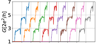
Figure 7: Conductance curves for single disorder configurations in the armchair case for $U_{0}=0.1t$. At the conductance plateaus, random fluctuations eventually cancel each other out, whereas the dip near the conductance step is in common to most disorder configurations, therefore it does not average out.

In Fig. 7 we show conductance curves of single disorder configurations. It can be seen that the dip at the conductance step is in common to most realizations. This is because most disordered energy landscapes have room for quasi-bound states within certain local energy wells. These states, lying at energies just under the opening of the next VP mode, couple to the propagating mode, which therefore localises at that energy, thereby decreasing the conductance.

To have a qualitatively better understanding of what causes the dips that we systematically observe in the conductance curves for a disordered system, we have performed additional numerical simulations. Suspecting these minima are due to the coupling of the VP modes to quasi-bound states in the system, we run simulations in the more conventional setting of a clean nanoribbon with a single attractive impurity. In this case, we put a single impurity on each edge, shifted away from the edge by the same amount. This makes the impurity on each edge interact with the same VP mode. The impurity has a Gaussian shape

$$U_{0}(\bm{\zeta})=u_{0}\,e^{-\frac{(\bm{\zeta}-\bm{\zeta}_{\text{L}})^{2}+(\bm{\zeta}-\bm{\zeta}_{\text{R}})^{2}}{2\sigma}},$$

centered at $\bm{\zeta}_{\text{L}}=(x_{\text{L}},y_{\text{L}})$ on one edge and $\bm{\zeta}_{R}=(x_{\text{R}},y_{\text{R}})$ on the other edge. The impurity is therefore fully characterised by its position, strength $u_{0}<0$, and width $\sigma$ (or variance $\sigma^{2}$). As discussed in the main text, we indeed observe dips in the conductance near the steps. How many dips we see, at which steps, and their shape, depend on the properties of the impurities. For impurities that are very narrow, such as $\sigma=a_{0}$, we observe dips only at certain steps, and not at others, depending on where the impurity lies — c.f. Fig. 8(b). For wider impurities, such as $\sigma=3a_{0}$, we observe dips at all steps, as well as other dips in the plateaus — c.f. Fig. 8(a). Additional dips can result from having multiple evanescent modes at the impurity due to its finite width, or geometrical resonance effects. For the case of quasi-one dimensional quantum wires, it is also known that in the presence of Rashba SOC Bercioux and Lucignano (2015) the dips never go all the way down to the level of the previous conductance step, but are lifted proportional to the forth order in the Rashba SOC parameter Pascual Gil et al. (2020). A systematic study of all these features is left to future investigations.

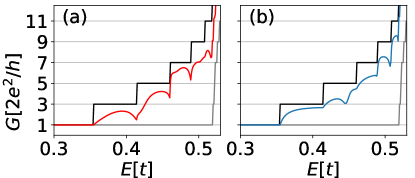
Figure 8: Conductance for a clean system containing one Gaussian shaped impurity on each edge. In (a) $\sigma=3a_{0}$ and in (b) $\sigma=a_{0}$, with $u_{0}=-0.4t$ and positions $x_{L}=x_{R}=L_{x}/2$, and $y_{L}=8.848a_{0}$ and $y_{R}=L_{y}-y_{L}$. In (a), due to the width of the impurity, all propagating VP modes couple to the evanescent mode at the impurity. In (b), because the impurity potential is much narrower, certain propagating modes do not interact with the evanescent mode at the impurity.

References

- Kane and Mele (2005a) C. L. Kane and E. J. Mele, Phys. Rev. Lett. 95, 146802 (2005a).
- Kane and Mele (2005b) C. L. Kane and E. J. Mele, Phys. Rev. Lett. 95, 226801 (2005b).
- Sichau et al. (2019) J. Sichau, M. Prada, T. Anlauf, T. J. Lyon, B. Bosnjak, L. Tiemann, and R. H. Blick, Phys. Rev. Lett. 122, 046403 (2019).
- Weeks et al. (2011) C. Weeks, J. Hu, J. Alicea, M. Franz, and R. Wu, Phys. Rev. X 1, 021001 (2011).
- Swartz et al. (2013) A. G. Swartz, J.-R. Chen, K. M. McCreary, P. M. Odenthal, W. Han, and R. K. Kawakami, Phys. Rev. B 87, 075455 (2013).
- Jia et al. (2015) Z. Jia, B. Yan, J. Niu, Q. Han, R. Zhu, D. Yu, and X. Wu, Phys. Rev. B 91, 085411 (2015).
- Chandni et al. (2015) U. Chandni, E. A. Henriksen, and J. P. Eisenstein, Phys. Rev. B 91, 245402 (2015).
- Hatsuda et al. (2018) K. Hatsuda, H. Mine, T. Nakamura, J. Li, R. Wu, S. Katsumoto, and J. Haruyama, Science Advances 4, eaau6915 (2018).
- Gmitra and Fabian (2015) M. Gmitra and J. Fabian, Phys. Rev. B 92, 155403 (2015).
- Wang et al. (2015) L. Wang, I. Gutiérrez-Lezama, C. Barreteau, N. Ubrig, E. Giannini, and A. F. Morpurgo, Nat. Commun. 6, 8892 (2015).
- Wang et al. (2016) Z. Wang, D.-K. Ki, J. Y. Khoo, D. Mauro, H. Berger, L. S. Levitov, and A. F. Morpurgo, Phys. Rev. X 6, 041020 (2016).
- Frank et al. (2018) T. Frank, P. Högl, M. Gmitra, D. Kochan, and J. Fabian, Phys. Rev. Lett. 120, 156402 (2018).
- Wakamura et al. (2019) T. Wakamura, F. Reale, P. Palczynski, M. Q. Zhao, A. T. C. Johnson, S. Guéron, C. Mattevi, A. Ouerghi, and H. Bouchiat, Phys. Rev. B 99, 245402 (2019).
- Island et al. (2019) J. O. Island, X. Cui, C. Lewandowski, J. Y. Khoo, E. M. Spanton, H. Zhou, D. Rhodes, J. C. Hone, T. Taniguchi, K. Watanabe, L. S. Levitov, M. P. Zaletel, and A. F. Young, Nature 571, 85 (2019).
- Tiwari et al. (2020) P. Tiwari, S. K. Srivastav, S. Ray, T. Das, and A. Bid, “Quantum spin hall effect in bilayer graphene heterostructures,” (2020), arXiv:2003.10292 .
- Liu et al. (2011) C.-C. Liu, H. Jiang, and Y. Yao, Phys. Rev. B 84, 195430 (2011).
- Molle et al. (2017) A. Molle, J. Goldberger, M. Houssa, Y. Xu, S.-C. Zhang, and D. Akinwande, Nat. Mater. 16, 163 (2017).
- Reis et al. (2017) F. Reis, G. Li, L. Dudy, M. Bauernfeind, S. Glass, W. Hanke, R. Thomale, J. Schäfer, and R. Claessen, Science 357, 287 (2017).
- Deng et al. (2018) J. Deng, B. Xia, X. Ma, H. Chen, H. Shan, X. Zhai, B. Li, A. Zhao, Y. Xu, W. Duan, S.-C. Zhang, B. Wang, and J. G. Hou, Nat. Mater. 17, 1081 (2018).
- Yang et al. (2012) F. Yang, L. Miao, Z. F. Wang, M.-Y. Yao, F. Zhu, Y. R. Song, M.-X. Wang, J.-P. Xu, A. V. Fedorov, Z. Sun, G. B. Zhang, C. Liu, F. Liu, D. Qian, C. L. Gao, and J.-F. Jia, Phys. Rev. Lett. 109, 016801 (2012).
- Sabater et al. (2013) C. Sabater, D. Gosálbez-Martínez, J. Fernández-Rossier, J. G. Rodrigo, C. Untiedt, and J. J. Palacios, Phys. Rev. Lett. 110, 176802 (2013).
- Drozdov et al. (2014) I. K. Drozdov, A. Alexandradinata, S. Jeon, S. Nadj-Perge, H. Ji, R. J. Cava, B. Andrei Bernevig, and A. Yazdani, Nat. Phys. 10, 664 (2014).
- Li et al. (2018) G. Li, W. Hanke, E. M. Hankiewicz, F. Reis, J. Schäfer, R. Claessen, C. Wu, and R. Thomale, Phys. Rev. B 98, 165146 (2018).
- Pulkin and Yazyev (2019) A. Pulkin and O. V. Yazyev, “Controlling the quantum spin hall edge states in two-dimensional transition metal dichalcogenides,” (2019), arXiv:1907.12481 .
- Wakamura et al. (2018) T. Wakamura, F. Reale, P. Palczynski, S. Guéron, C. Mattevi, and H. Bouchiat, Phys. Rev. Lett. 120, 106802 (2018).
- Volkov and Pankratov (1985) B. A. Volkov and O. A. Pankratov, JETP Lett. 42, 178 (1985).
- Pankratov et al. (1987) O. A. Pankratov, S. V. Pakhomov, and B. A. Volkov, Solid State Commun. 61, 93 (1987).
- Pankratov (2018) O. A. Pankratov, Physics-Uspekhi 61, 1116 (2018).
- Inhofer et al. (2017) A. Inhofer, S. Tchoumakov, B. A. Assaf, G. Fève, J. M. Berroir, V. Jouffrey, D. Carpentier, M. O. Goerbig, B. Plaçais, K. Bendias, D. M. Mahler, E. Bocquillon, R. Schlereth, C. Brüne, H. Buhmann, and L. W. Molenkamp, Phys. Rev. B 96, 195104 (2017).
- Tchoumakov et al. (2017) S. Tchoumakov, V. Jouffrey, A. Inhofer, E. Bocquillon, B. Plaçais, D. Carpentier, and M. O. Goerbig, Phys. Rev. B 96, 201302 (2017).
- Mahler et al. (2019) D. M. Mahler, J.-B. Mayer, P. Leubner, L. Lunczer, D. Di Sante, G. Sangiovanni, R. Thomale, E. M. Hankiewicz, H. Buhmann, C. Gould, and L. W. Molenkamp, Phys. Rev. X 9, 031034 (2019).
- Lu and Goerbig (2019) X. Lu and M. O. Goerbig, EPL (Europhysics Letters) 126, 67004 (2019).
- van den Berg et al. (2020) T. L. van den Berg, M. R. Calvo, and D. Bercioux, Phys. Rev. Research 2, 013171 (2020).
- Alspaugh et al. (2020) D. J. Alspaugh, D. E. Sheehy, M. O. Goerbig, and P. Simon, Phys. Rev. Research 2, 023146 (2020).
- Bagwell (1990) P. F. Bagwell, Phys. Rev. B 41, 10354 (1990).
- Brey and Fertig (2006) L. Brey and H. A. Fertig, Phys. Rev. B 73, 235411 (2006).
- Castro Neto et al. (2009) A. H. Castro Neto, F. Guinea, N. M. R. Peres, K. S. Novoselov, and A. K. Geim, Rev, Mod. Phys. 81, 109 (2009).
- Landau and Lifshitz (1986) L. Landau and E. Lifshitz, Quantum Mechanics (Elsevier, 1986).
- Olver et al. (2010) F. W. Olver, D. W. Lozier, R. F. Boisvert, and C. W. Clark, eds., NIST Handbook of Mathematical Functions (Cambridge University Press, 2010).
- Wakabayashi et al. (2010) K. Wakabayashi, K. ichi Sasaki, T. Nakanishi, and T. Enoki, Science and Technology of Advanced Materials 11, 054504 (2010).
- Groth et al. (2014) C. W. Groth, M. Wimmer, A. R. Akhmerov, and X. Waintal, New J. Phys. 16, 063065 (2014).
- Tekman and Bagwell (1993) E. Tekman and P. F. Bagwell, Physical Review B 48, 2553 (1993).
- Palacios and Tejedor (1993) J. J. Palacios and C. Tejedor, Physical Review B 48, 5386 (1993).
- Haug (1993) R. J. Haug, Semiconductor Science and Technology 8, 131 (1993).
- Chu and Sorbello (1989) C. S. Chu and R. S. Sorbello, Phys. Rev. B 40, 5941 (1989).
- Groth et al. (2009) C. W. Groth, M. Wimmer, A. R. Akhmerov, J. Tworzydło, and C. W. J. Beenakker, Phys. Rev. Lett. 103, 196805 (2009).
- Jiang et al. (2009) H. Jiang, L. Wang, Q.-f. Sun, and X. C. Xie, Phys. Rev. B 80, 165316 (2009).
- Wu et al. (2016) B. Wu, J. Song, J. Zhou, and H. Jiang, Chin. Phys. B 25, 117311 (2016).
- Bloch et al. (2008) I. Bloch, J. Dalibard, and W. Zwerger, Rev. Mod. Phys. 80, 885 (2008).
- Haldane (1988) F. D. M. Haldane, Phys. Rev. Lett. 61, 2015 (1988).
- Tarruell et al. (2012) L. Tarruell, D. Greif, T. Uehlinger, G. Jotzu, and T. Esslinger, Nature 483, 302 (2012).
- Jotzu et al. (2014) G. Jotzu, M. Messer, R. Desbuquois, M. Lebrat, T. Uehlinger, D. Greif, and T. Esslinger, Nature 515, 237 (2014).
- Goldman et al. (2010) N. Goldman, I. Satija, P. Nikolic, A. Bermudez, M. A. Martin-Delgado, M. Lewenstein, and I. B. Spielman, Phys. Rev. Lett. 105, 255302 (2010).
- Bercioux et al. (2011) D. Bercioux, N. Goldman, and D. F. Urban, Phys. Rev. A 83, 023609 (2011).
- Goldman et al. (2011) N. Goldman, D. F. Urban, and D. Bercioux, Phys. Rev. A 83, 063601 (2011).
- Goldman et al. (2016) N. Goldman, G. Jotzu, M. Messer, F. Görg, R. Desbuquois, and T. Esslinger, Phys. Rev. A 94, 043611 (2016).
- Buchhold et al. (2012) M. Buchhold, D. Cocks, and W. Hofstetter, Phys. Rev. A 85, 063614 (2012).
- Bercioux and Lucignano (2015) D. Bercioux and P. Lucignano, Rep. Progr. Phys. 78, 106001 (2015).
- Pascual Gil et al. (2020) A. Pascual Gil, T. L. van den Berg, V. N. Golovach, J. J. Sáenz, and S. Bergeret, “Quasi-bound states in a nanowire as an interference probe of the SU(2) gauge field,” (2020), In preparation.