A global view on the colliding-wind binary WR 147 

Abstract

We present results from a global view on the colliding-wind binary WR 147. We analysed new optical spectra of WR 147 obtained with Gran Telescopio CANARIAS and archive spectra from the Hubble Space Telescope by making use of modern atmosphere models accounting for optically thin clumping. We adopted a grid-modelling approach to derive some basic physical characteristics of both stellar components in WR 147. For the currently accepted distance of 630 pc to WR 147, the values of mass-loss rate derived from modelling its optical spectra are in acceptable correspondence with that from modelling its X-ray emission. However, they give a lower radio flux than observed. A plausible solution for this problem could be if the volume filling factor at large distances from the star (radio-formation region) is smaller than close to the star (optical-formation region). Adopting this, the model can match well both optical and thermal radio emission from WR 147. The global view on the colliding-wind binary WR 147 thus shows that its observational properties in different spectral domains can be explained in a self-consistent physical picture.

1 Introduction

Massive stars of early type, Wolf-Rayet (WR) and OB, possess massive and fast supersonic stellar winds: typically $\dot{M}\sim 10^{-5}$ (WR) and $\sim 10^{-7}-10^{-6}$ (OB) M_⊙ yr^-1 and $V_{wind}=1000-5000$ km s^-1. If both components of a binary system are massive stars, their powerful winds will interact resulting in enhanced X-ray emission, produced in the colliding-stellar-wind (CSW) shocks, as first proposed by Prilutskii & Usov (1976) and Cherepashchuk (1976). However, the CSW role is not limited to the X-ray emission of massive binaries. For example, wide WR+OB binaries are non-thermal radio sources (Dougherty & Williams, 2000) and this emission is believed to originate from their CSW region. Also, CSWs are invoked to explain the recurrent infrared bursts observed in the so called episodic dust makers, which are wide WR+O binaries with high orbital eccentricity (Williams 1995, Williams 2008 and references therein).

We note that the basic parameters that determine the physical characteristics of the shocked CSW plasma are the mass-loss rate and velocity of the stellar winds and the binary separation (Lebedev & Myasnikov 1990; Luo et al. 1990; Stevens et al. 1992; Myasnikov & Zhekov 1993). Since the bulk emission of the CSW plasma is in X-rays, comparison of observed X-ray spectra of wide CSW binaries with theoretical predictions could provide additional constraints on the stellar wind properties of the binary components.

Interestingly, the direct modelling of the X-ray emission from the wide WR+O binaries WR 137, WR 146 and WR 147 in the framework of the CSW picture required mass-loss rate lower than the currently accepted values for these objects: of about one order of magnitude for WR 137 and WR 146, and of about a factor of four for WR 147 (Zhekov 2015; Zhekov 2017; Zhekov & Park 2010b). Similarly, reduced mass-loss rates of the stellar components by a factor of $\sim 7.5-7.7$ was deduced from a direct modelling of the X-ray emission of the O$+$O binary Cyg OB2 9 (Schulte 9; Parkin et al. 2014).

In order to find a solution to this problem, a global view on the spectral modelling was proposed (for details see section 5 in Zhekov 2017). Namely, we need to carry out spectral modelling of the observational properties of massive stars in different spectral domains (e.g., radio, optical/UV, X-ray) to see whether we could reconcile the results on mass-loss rates from different analyses.

In this study, we chose to adopt a global view on the WR+OB binary WR 147: it is a classical CSW binary; it has been studied in considerable detail almost along the entire spectrum; it has the smallest mass-loss mismatch amongst the studied CSW binaries so far (see above). It is worth noting that WR 147 has been spatially resolved in each spectral domain: radio (Moran et al., 1989), infrared (Williams et al., 1997), optical (Niemela et al., 1998), X-rays (Zhekov & Park, 2010a). This could potentially allow for obtaining observational properties of both stellar components in this CSW binary: a WN8 Wolf-Rayet star and an OB star.

Our paper is organized as follows. In Section 2, we describe the new and archival optical observations of WR 147. In Section 3, we give details about the modelling of the optical spectra of both binary components and the corresponding results. In Section 4, we discuss our results, and we present our conclusions in Section 5.

Figure 1: Examples of the spectral ‘deconvolution’. The two-Gaussian fit results are shown in the first row. The data are depicted with ‘+’ sign and dashed line; the fit components are shown with dotted lines. Results from the Richardson-Lucy deconvolution (solid line) are shown in the second row . The three columns (from left to right show the cross-dispersion cuts at $\lambda=5000$ Å, $\lambda=6000$ Å  and $\lambda=7000$ Å, respectively.

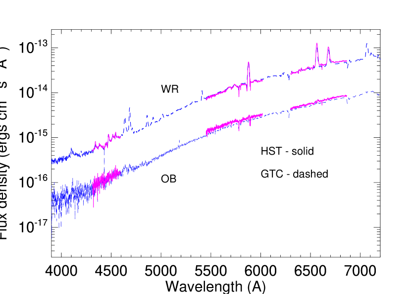
Figure 2: The HST vs. GTC comparison of the mean spectra of the WR and OB components in WR 147. The HST and GTC spectra are in magenta and blue color, respectively.

2 Observations and data reduction

2.1 Observations with Gran Telescopio CANARIAS

WR 147 was observed with Gran Telescopio CANARIAS on 2017 September 18 under excellent photometric conditions (clear skies and seeing of $\approx 0\aas@@fstack{\prime\prime}6$; see also Section 2.1.1). The long-slit mode of the OSIRIS spectrograph was used in combination with the R1000B grism that provides spectra in the 3630 - 7500 Å  range with a resolution of $\lambda/\Delta\lambda\approx 1018$. The slit width was $0\aas@@fstack{\prime\prime}6$ and the slit length was aligned with the position angle of the WR 147 binary (PA $=-10\degr$; see table 2 in Niemela et al. 1998). Twelve scientific exposures of WR 147 were carried out with this OSIRIS setup. However, two of them (exposure time of 180 and 360 s) resulted in saturated spectra at wavelengths $>\,\sim 6000$ Å. So, only ten spectra (each with a 90-s exposure time) were used in the current analysis.

Following the standard calibration procedure for OSIRIS, the calibration frames were acquired at the end of the observing night, utilizing the Naysmith B focal station Instrument Calibration Module (ICM) and the same instrument configuration. This calibration approach is feasible due to the proven stability of OSIRIS and has been validated all through the instrument operation.

For the flux calibration, we used spectra of the spectrophotometric standard star G191-B2B, obtained in the same night with the same instrument configuration and under similar observing conditions through a $2\aas@@fstack{\prime\prime}5$ wide long-slit. Thus assuring that all the flux from the standard star has passed through the observing system and reached the instrument detector.

For the flat field corrections, wavelength calibration and correcting the distortion, we used the standard iraf  tasks in the twospec package. We note that individual spectra of the WR and OB components in WR 147 were extracted first (see Section 2.1.1) and then flux-calibrated.

2.1.1 Spectral ‘deconvolution’

Given the brightness difference between the WR and OB components in WR 147 of about 2 mag in the V-filter and the measured angular separation of $0\aas@@fstack{\prime\prime}64$ (Niemela et al., 1998), we opted out for the $1\times 1$ binning detector readout mode, instead of the nominal $2\times 2$ binning of OSIRIS. Nevertheless, the resulting pixel size is still $0\aas@@fstack{\prime\prime}125$ and we had to adopt some ‘deconvolution’ technique aimed at extracting a separate spectrum for the WR and OB component, respectively.

As a first step, we performed a ’spatial’ fit (i.e., in the cross-dispersion direction) at each ‘spectral’ bin (wavelength) of the GTC-OSIRIS data of WR 147. The model function consisted of two Gaussian components and a continuum. The fit parameters were total flux and position of each component, the Gaussian $\sigma$ (being the same for both components) and the continuum level.

To check our ‘deconvolution’ approach, the Richardson-Lucy algorithm was used as well. It revealed that two components do exist in the OSIRIS data in the cross-dispersion direction.

Interestingly, the results from our two-component fits and the Richardson-Lucy deconvolution (Richardson 1972; Lucy 1974) showed that we do find two spectral components that are separated at $\sim$ 0$\aas@@fstack{\prime\prime}$6 - 0$\aas@@fstack{\prime\prime}$7 in ‘spatial’ (cross-dispersion) direction and the ‘southern’ component (WR star) is brighter. Just to recall that the separation of the two stellar components in WR 147 is 0$\aas@@fstack{\prime\prime}$64$\pm$0$\aas@@fstack{\prime\prime}$16 (Niemela et al., 1998). Figure 1 presents some results from our deconvolution experiment.

All this gave us confidence to proceed with the two-Gaussian spectral ‘deconvolution’ of the GTC-OSIRIS data of WR 147. A fixed separation between the two components of 0$\aas@@fstack{\prime\prime}$64 was adopted in these fits. Thus, the GTC-OSIRIS spectra were subject to our ‘deconvolution’ procedure and the WR and OB spectra were extracted for each data set. To increase the signal-to-noise in the spectra, all the 90-sec-exposure spectra were combined which resulted in a mean spectrum for each stellar component in WR 147.

Finally, the mean GTC spectrum of each stellar component was corrected for the loss of flux that fell outside the spectrograph slit. This was done by adopting a 2-D Gaussian PSF (point-spread function) and estimating the fraction of the seeing that fell in the slit. An average seeing of 0$\aas@@fstack{\prime\prime}$70$\pm$0$\aas@@fstack{\prime\prime}$03 (FWHM) was derived for the 90-sec data, which is the mean value of the spatial component shape as derived from our ‘deconvolution’ procedure for each data set (for comparison, the Differential Image Motion Monitor at the Las Moradas site located 300 meters East from the GTC, also known as IAC-DIMM, gave an average seeing of 0$\aas@@fstack{\prime\prime}$74$\pm$0$\aas@@fstack{\prime\prime}$04 for the same night). This estimate showed that a fraction of 0.844 of the total flux from WR 147 fell into the spectrograph slit, therefore, a correction coefficient of 1.184 was adopted for the GTC spectra of WR 147.

Figure 2 shows how the GTC spectra of WR 147 compare with those from the Hubble Space Telescope (HST). We note the good correspondence between the two data sets and we underline that the HST data allow for a standard spectral extraction of the WR and OB components (see Section 2.2), that is, no ‘deconvolution’ technique has been adopted in that case. Thus, we feel confident to proceed further with the spectral analysis of the GTC data on WR 147.

2.2 Archive data from the Hubble Space Telescope

For the purpose of this study, we made use of archival data from the Hubble Space Telescope that provide spatially resolved spectra of both binary components in WR 147. The long-slit spectroscopy of WR 147 was obtained with STIS (Space Telescope Imaging Spectrograph) in combination with the G430M and G750M gratings (Obs IDs: o5d503010, o5d503020 and o5d503040), which provide spectra in the 3020-5610 Å  ($\lambda/\Delta\lambda=5390-10020$) and 5450-10140 Å  ($\lambda/\Delta\lambda=4870-9050$) range, respectively. These archival spectra are flux-calibrated and we note that they were already discussed by Lépine et al. (2001). As noted by these authors, the two stars in the WR 147 system are clearly resolved, which allows for using standard iraf aperture extraction to obtain their spectra. We thus adopted the same approach for the spectral extraction.

3 Spectral modelling

3.1 The stellar atmosphere model

For the purposes of our investigation, we employ the non-LTE radiative transfer code cmfgen (Hillier & Miller 1999; Hillier & Lanz 2001), which is a fully line-blanketed atmosphere code, designed to solve the statistical equilibrium and radiative transfer equations in spherical geometry.

The basic input parameters are stellar mass, luminosity, effective temperature, mass-loss rate, wind velocity and chemical composition (H, He, C, N, O, Ne, Mg, Al, Si, P, S, Ar, Ca, and Fe abundances; for model atoms see Table 2 in Appendix B). Stellar effective temperature in cmfgen is defined using the Stefan-Boltzmann law with reference radius, $R_{2/3}$, specified for the Rosseland opacity of 2/3: T_∗ $=(L/4\pi R^{2}_{2/3})^{1/4}$, where $L$ is the stellar luminosity.

Observations indicate that stellar winds of massive stars are not homogeneous, instead the stellar winds contain inhomogeneities or clumps. These clumps affect the stellar spectra and therefore modelling non-homogeneous stellar atmospheres is required.

cmfgen can take optically thin clumping (microclumping) into account. Microclumping approach is based on the hypothesis that the wind consists of ‘clumps’, which have enhanced density and dimension smaller than the photon mean free path. The density of the clumps is enhanced by a clumping factor $D$, compared to the mean density of the wind. This factor is described by the volume filling factor with relation $f=1/D$, assuming that the inter-clump medium is void. Our models are calculated with distant variable volume filing factor $f_{\infty}=0.1$, prescribed by the following law (see eq. 5 in Hillier & Miller 1999):

$$f(r)=f_{\infty}+(1-f_{\infty})\exp[-\varv(r)/\varv_{cl}]$$ (1)

where, $v_{cl}$ is the velocity at which clumping starts. We have chosen the clumping to start at $\varv_{cl}=30$  km s^-1, which is near the sonic point.

It should be stated that cmfgen does not currently solve the wind momentum equation. Therefore, the wind velocity structure has to be adopted. In our models, the wind velocity structure is described by a standard $\beta$-type velocity law with exponent $\beta=1$. The velocity law is joined to the hydrostatic part of the wind just below the sonic point, where the wind speed reaches local speed of sound.

The choice of having single values for the volume filling factor and the velocity-law exponent is aimed at minimizing the number of free parameters in the models (see Section 3.2). The specific choice of $f_{\infty}=0.1$ and $\beta=1$ is based on a previous study of the optical-IR spectra of WR 147 by Morris et al. (2000). These parameter values could be considered standard in spectral modelling of massive Wolf-Rayet stars (e.g., Hamann et al. 2006; Sander et al. 2012).

3.2 Grid modelling

We recall that the purpose of the spectral modelling by making use of stellar atmosphere models (e.g., the cmfgen code) is to derive some basic physical characteristics of the studied massive stars: e.g., the mass-loss rate ($\dot{M}$), luminosity (L), effective temperature (T_∗). It is well known, but it is nevertheless worth recalling that the spectrum of a massive star is determined by the ionization structure of its wind. In general, the ionization structure at a given point in the stellar wind depends on the ratio of the ionizing photons to the gas number density. The bulk of ionizing photons is determined by both the stellar luminosity and the stellar temperature (controlling the shape of the underlying continuum). On the other hand, the mass-loss rate of the massive star is the main factor that sets the gas number density.

Therefore, we fit an observed spectrum directly (i.e., performing a full spectral comparison) in order to derive these specific stellar parameters: $\dot{M}$, L, T_∗. Since the observed spectrum is flux-calibrated, we need to specify the distance to the studied object and to take into account the interstellar absorption. As a result, the fit provides the best value for the quantity E(B-V) adopting the standard ISM extinction curve ($R_{V}=3.1$) of Fitzpatrick (1999). We next discuss a few important items for our fitting procedure.

(i) We note that all the spectral fits were done by making use of the Levenberg-Marquardt method for non-linear $\chi^{2}$ fitting, which via iterations finds the best fit (the minimum $\chi^{2}$ value) and requires an estimate of the theoretical function at each iteration (e.g., section 15.5 in Press et al. 1992). Since it is not feasible to directly calculate a theoretical (unabsorbed) spectrum for a given set of stellar parameters (too long a computational time), the theoretical spectrum for each iteration is based on a preliminarily built grid of model spectra for a specific range of values of each of the stellar parameters of interest: i.e., $\log~{}\dot{M}$, $\log$ L and T_∗. So, at each iteration we first find in which cell of the 3-D model grid the current parameter set ($\log~{}\dot{M}$, $\log$ L, T_∗) is located. Then the resultant spectrum is estimated by interpolating (with specific weights = inverse distance-square) between all the model spectra which define that grid cell (eight spectra in total). This interpolation is similar to the Shepard’s method (Shepard, 1968) but it is adopted locally:

$$Sp=\sum_{i=1}^{8}w_{i}Sp_{i},\hskip 28.45274ptw_{i}=\frac{\frac{1}{l_{i}^{2}}}{w_{tot}},\hskip 28.45274ptw_{tot}=\sum_{i=1}^{8}\frac{1}{l_{i}^{2}}$$

where $l_{i}$ is the distance from the point ($\log~{}\dot{M}$, $\log$ L, T_∗) in the 3-D parameter space to each of the eight spectra ($Sp_{i}$) that correspond to the vertexes of the current grid cell. We note that the axes of the model grid are dimensionless and span the range [0, 1], that is each parameter is normalized to its range: $\bar{p}=(p-p_{min})/(p_{max}-p_{min})$, where $p$ is a given parameter and $p_{min},p_{max}$ are its minimum and maximum values, and $\bar{p}\in[0,1]$. Thus, all the physical parameters of the model grid are ‘equal’ in defining the distance in the 3-D parameter space.

(ii) We recall that the Levenberg-Marquardt method is a non-linear $\chi^{2}$ fitting method and thus requires an initial guess of the model parameters. Also, due to the complex topology of the $\chi^{2}$- surface of the non-linear methods very often a local minimum is found that may not be the true minimum we are looking for. To circumvent this issue, we adopted the following approach in our grid modelling.

We create a large number of initial parameter sets by randomly choosing parameter values in the grid range for each parameter. For each set of initial parameters, the Levenberg-Marquardt method finds the corresponding ‘best fit’, which is characterized by its $\chi^{2}$ value. We find the minimum value amongst all the $\chi^{2}$ values (a great number of them, e.g., 10 000 or so), thus, starting from that particular set of initial parameters, we find the parameters of the spectral model that provide the best fit to the observed spectrum: ($\log~{}\dot{M}$, $\log$ L, T_∗)_best.

(iii) As a final check, we calculate the theoretical model directly with cmfgen by using exactly these ‘best-fit’ parameters derived from the grid fitting and use it to fit the observed spectrum.

Figure 3: Some best-fit results from the grid-modelling of the GTC spectra of WR 147. The dependence of the mass-loss rate, stellar luminosity and absolute visual magnitude on the adopted distance to WR 147 is shown in the first three rows. Error bars ($1\sigma$ errors from the fits) are smaller than the plot symbols denoting them, except for the mass-loss rate and luminosity of the OB component.

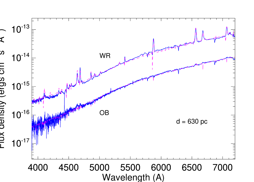
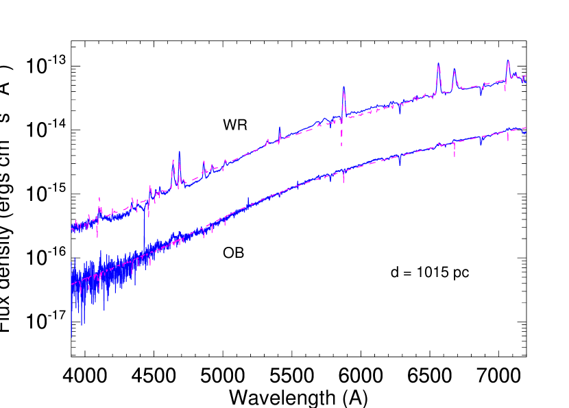
Figure 4: Examples of the observed GTC spectra (blue solid line) overlaid with the best-fit model (magenta dashed line).

Figure 5: The same as in Fig. 3 but for the grid-modelling of the HST spectra of WR 147.

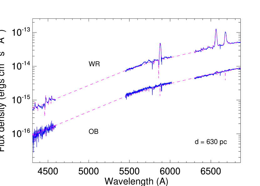
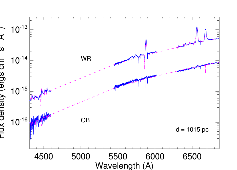
Figure 6: Examples of the observed HST spectra (blue solid line) overlaid with the best-fit model (magenta dashed line).

3.3 Results

For fitting the observed GTC and HST spectra of WR 147 (WN8$+$B0.5 - O9; e.g., Niemela et al. 1998), we adopted a uniform approach for modelling the stellar spectra of both binary components. So, we have built two grids of model spectra that are representative for WN8 and OB objects, respectively, and consider the following stellar parameters: mass-loss rate $\log~{}\dot{M}$ (in units of solar masses per year,  M_⊙ yr^-1 ), stellar luminosity $\log$ L (in units of solar luminosity,  L_⊙ ) and effective temperature T_∗ (in Kelvin). The grids are based on 80 and 60 model spectra for the WN8 and OB star, respectively. All models have a spectrum-formation zone with an inner radius corresponding to the Rosseland opacity of 100 and an outer radius of a hundred inner radii. The ranges of the basic stellar parameters are as follows.

For the WN8 grid, we have $\log~{}\dot{M}$ $=[-5.0,~{}-4.8,~{}-4.5,~{}-4.3]$, $\log$ L $=[5.0,~{}5.2,~{}5.4,~{}5.6,~{}5.8]$, T_∗ $=[32500,~{}35000,~{}37500,~{}40000]$. The adopted chemical abundances of H and He are those from Morris et al. (2000) and for all other elements are from van der Hucht et al. (1986). The stellar wind velocity is 1000 km s^-1 corresponding to the range of wind velocity values $950-1100$ km s^-1 derived from observations of WR 147 (Eenens & Williams 1994; Hamann et al. 1995; Morris et al. 2000).

For the OB grid, we have $\log~{}\dot{M}$ $=[-7.0,~{}-6.8,~{}-6.3]$, $\log$ L $=[4,2,~{}4.5,~{}4.8,~{}5.0,~{}5.5]$, T_∗ $=[27500,~{}30000,~{}32500,~{}35000]$, the abundances are solar (Asplund et al., 2009) and the stellar wind velocity is 1600 km s^-1 representative of the range of wind velocity values typical for a B0.5 - O9 massive star (e.g., Prinja et al. 1990; Prinja & Crowther 1998).

The currently accepted distance to WR 147 is $630\pm 70$ pc (Churchwell et al., 1992) but it is a photometric distance, so, we explore a range of values for this parameter. Namely, we consider six different values starting with d $=630$ pc and each consecutive value increases by 10%. Thus, we could explore how the stellar parameters derived from the model fitting depend on the adopted distance to WR 147. It is worth noting that the Gaia parallax of WR 147 is negative ($-1.2733\pm 0.3144$; Gaia Collaboration et al. 2018) likely due to the binary nature of this object. As a result, the Gaia distance to this object is not well constrained yet: it is much larger than the currently accepted distance to WR 147 and with large uncertainties (d $=4168^{+1619}_{-1174}$ pc; Bailer-Jones et al. 2018).

Based on each best-fit spectrum, we also calculated some synthetic magnitudes: the Johnson B and V, and the corresponding intrinsic colour $(B-V)_{0}$ and absolute visual magnitude M_V. For these, we made use of the filter response functions from Bessell & Murphy (2012) and zero points from Casagrande & VandenBerg (2014).

Anticipating the results from the grid-modelling, we note that exploring the entire OB grid in a standard way (i.e., fitting for all grid parameters, $\log~{}\dot{M}$, $\log$ L, T_∗) did not provide well constrained fit results for the OB star, due to the lack of strong spectral feature in its spectrum. So, to obtain some constraints on its physical parameters, we ran three different series of models each having a fixed value of the stellar temperature; namely, T${}_{*}=30.0,~{}32.5,~{}35.0$ kK.

Results from the grid-modelling of the GTC and HST spectra of WR 147 are presented in Figures 3, 5 and Table 1. The following things are worth mentioning.

We see that the derived stellar parameters in general follow the theoretically expected (approximate) correlations with the distance to the studied object: e.g., $\dot{M}\propto d^{1.5}$, $L\propto d^{2}$ (see eqs. 1 and 4 in Hillier & Miller 1999; also Schmutz et al. 1989) and the absolute visual magnitude has its standard dependence on distance: M${}_{V}\propto 5\log d$.

The values of the stellar temperature of the WR component are very similar for the fits to the GTC and HST spectra, thus, indicating a stellar temperature of the WN8 star in WR 147 of T${}_{*}\sim 37$ kK. And, the same is valid for the OB star in this binary, T${}_{*}\sim 32.5$ kK.

Also, the values for the interstellar extinction, derived from the fits to the spectra of the WR component in WR 147 (Table 1), A${}_{V}=3.1E(B-V)=10.42-10.54$ mag, correspond well to that adopted for this object in the VII-th Catalogue of Galactic Wolf-Rayet stars (A${}_{v}=1.11$ A_V and table 28 in van der Hucht 2001): namely A${}_{v}=11.57-11.70$ mag vs. A${}_{v}=11.60$ mag. On the other hand, the fits to the spectra of the OB component in WR 147 give a slightly higher value of the interstellar extinction (A${}_{v}=12.04$ mag). But, we have to keep in mind that the quality of the OB-star spectra is not very high, especially in the blue region, and this could be the reason for such a difference.

It is worth noting that the interstellar extinction towards WR 147 might not be standard ($R_{V}\neq 3.1$). For example, based on analysis of optical and infrared data of WR 147 Morris et al. (2000) suggest a value of $R_{V}=2.7$. However, the wavelength range of the optical spectra in our study is not very large ($\sim 3000$ Å) which prevents constraining the $R_{V}$-value very well. We nevertheless explored the case of non-standard interstellar extinction with $R_{V}=2.7$ but it provided a poorer match to the observed spectra. We thus feel confident in adopting the standard interstellar extinction curve ($R_{V}=3.1$) in the current spectral modelling.

The GTC and HST synthetic magnitudes are in general consistent between each other. We also note that the synthetic V magnitudes are very similar to the observed ones reported by Niemela et al. (1998) from HST photometry. However, the synthetic B magnitudes are by $\sim 1$ mag brighter than those reported by these authors, which is likely due to the different response function of the filters.

On the other hand, the values of synthetic magnitudes in the Johnson V filter match well those observed (see last two rows in Table 1). The observed V magnitude values of the WR 147 system are from the ASAS-SN (All Sky Automated Survey for Supernovae) campaign for the period 2017 September 12 - 27 (e.g., Shappee et al. 2014; Kochanek et al. 2017), thus, bracketing the date of the GTC observation (2017 September 18): V(ASAS-SN) $=13.76\pm 0.03$ mag.

To broaden such a comparison, we calculated synthetic magnitudes for the Pan-STARRS survey (Panoramic Survey Telescope and Rapid Response System) following the definition of its photometric system and using the filter bandpasses from Tonry et al. (2012). The observed magnutides are from the first data release (Chambers et al., 2016). Also, we calculated synthetic Gaia magnitudes adopting the filter bassbands and zero points from Evans et al. (2018). The observed magnutides are from the Gaia Data Release 2 (DR2; Gaia Collaboration et al. 2018).

As seen from Fig. 7 and keeping in mind that our synthetic magnitudes are based on modelling two different spectral sets (GTC and HST ) as each spectral and photometric data set bears its own observational and systematic uncertainties, we think that the correspondence between the synthetic and observed magnitudes is at acceptable level.

So, all this gives us confidence in the results from the performed grid-modelling of the optical spectra of WR 147. We think that the stellar parameters of the WR component in WR 147 are acceptably well constrained while those of the OB component are not so well constrained. The latter is understandable given the quality of the spectra (both GTC and HST) of the OB star in WR 147. Nevertheless, we note that for the best-fit values of the intrinsic (B-V)₀ colour and the absolute visual magnitude M_V are typical for an OB object of B0.5 - O8 V spectral type (e.g., Schmidt-Kaler 1982): corresponding to the range of distances explored here.

We would also like to mention that modelling of the stellar spectra could in general provide information on the chemical composition of the emitting gas. However, there are no resonance lines in the optical spectra of WR 147, which does not allow deriving very accurate values for the chemical abundances. We thus only tried to derive an estimate of the nitrogen abundance: it is the most abundant light metal in the WN stars. We recall that Morris et al. (2000) derived a hydrogen-to-helium abundance (by number) of 0.4, adopted in our study. For the best-fit case from the grid modelling of the WN component in WR 147, we used the cmfgen code to get a theoretical spectrum only of nitrogen. By varying its contribution to the total spectrum, the fit of the observed spectrum gave an estimate of the nitrogen-to-helium abundance (by number): N / He $=4.4\pm 0.2\times 10^{-3}$.

Finally, we assume that the derived values of the stellar parameters from the fits to the GTC and HST spectra of WR 147 could in fact define a possible range of values (accuracy) for a given stellar parameter, assuming a fixed/known distance. Thus, although a given physical parameter may vary appreciably for the explored range of distances to WR 147 (see above), we note that for each distance value the accuracy of mass-loss rate of both stellar components is $\sim 0.1$ dex, that of the stellar luminosity is $\leq 0.1$ dex (WR) and $\sim 0.1-0.15$ dex (OB), and that of the absolute V magnitude is $\sim 0.15$ mag for both components.

Because the stellar parameters are key ingredients in the general physical picture of WR 147, specifically the mass-loss rate (see Section 4), it is interesting to compare the values derived in this study with those from previous analyses using stellar atmosphere models by Morris et al. (2000) and Hamann et al. (2019). For the distances adopted in those studies (650 pc in Morris et al. 2000; 1200 pc in Hamann et al. 2019, this value corresponds to their adopted value for the distance modulus of 10.4 mag) and the same volume filling factor ($f=0.1$), the mass-loss rate of Morris et al. (2000) is about 2 times higher and that from Hamann et al. (2019) is about 3 - 4 times higher than the value derived here. We think that one of the reasons for such differences is related to the fact that the absolute calibration of the models in the latter is based on adopting some absolute magnitude typical for the object (e.g., absolute $K$-magnitude in Morris et al. 2000; absolute $\varv$-magnitude in Hamann et al. 2019), while our grid modelling is based on fitting directly for the stellar luminosity. It is our understanding that fitting for luminosity should be physically reasonable. On the other hand, absolute magnitudes of Wolf-Rayet stars even of a given subclass may have an appreciable scatter (e.g., van der Hucht 2001; Rate & Crowther 2020). A limitation of our analysis is that it is based only on the optical spectra of WR 147, while both other studies take into consideration optical-infrared data. However, the good correspondence between the results of our modelling and observations of a range of facilities (e.g., see Fig. 7) gives us additional confidence in the derived results. But, we note that a factor of $\sim 2$ difference could in general reflect uncertainties typical for deriving mass-loss rates based on using stellar atmosphere models (e.g., based on different atomic data etc.).

Table 1: WR 147 Spectral Fit Results

Para-	WR		OB
meter	GTC	HST	GTC	HST
T∗	$36.9\pm 0.9$	$37.3\pm 0.8$	$30.0-35.0$	$30.0-35.0$
E(B-V)	$3.36\pm 0.01$	$3.40\pm 0.01$	$3.50\pm 0.01$	$3.50\pm 0.01$
(B-V)0	$-0.29\pm 0.01$	$-0.29\pm 0.01$	$-0.30\pm 0.01$	$-0.30\pm 0.01$
B	$16.86\pm 0.01$	$16.87\pm 0.01$	$19.02\pm 0.01$	$18.89\pm 0.01$
V	$13.92\pm 0.01$	$13.89\pm 0.01$	$15.99\pm 0.01$	$15.86\pm 0.01$
Vsys	$13.77\pm 0.01$ (GTC)		$13.72\pm 0.01$ (HST)
	$13.76\pm 0.03$ (ASAS-SN)

Note. Results from the fits to the optical spectra of WR 147. Tabulated parameters are the stellar temperature T_∗, interstellar extinction E(B-V), intrinsic colour (B-V)₀, B, V and total magnitude (WR$+$OB) of the system V_sys followed by the observed V magnitude from the ASAS-SN campaign. The value of T_∗ is in unit of kK ($10^{3}$ Kelvin) and all other parameters are in magnitudes. The errors are the standard deviation for the fit results of a given parameter as derived for the sample of six values of the distance to WR 147 (see text).

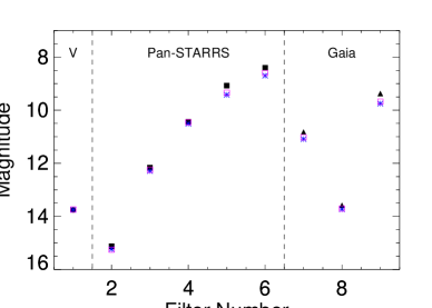
Figure 7: Comparison between synthetic and observed magnitudes of WR 147. The observed magnitudes are given with filled symbols: a circle for the V magnitude from the ASAS-SN campaign (filter number 1, $\lambda_{mean}=5500$ Å; $\lambda_{mean}=\sum\lambda T_{\lambda}/\sum T_{\lambda}$, $T_{\lambda}$ is the filter passband at wavelength $\lambda$); squares for the g, r, i, z , y magnitudes from the Pan-STARRS catalogue (filter numbers 2 - 6, $\lambda_{mean}=4866,6215,7545,8680,9633$ Å, respectively); triangles for the g, bp, rp magnitudes from the Gaia DR2 catalogue (filter numbers 7 - 9, $\lambda_{mean}=6406,5131,7777$ Å, respectively). The synthetic magnitudes for the best GTC and HST models are marked with asterisks (in blue) and open squares (in magenta), respectively.

4 Discussion

4.1 CSW picture

Global fits to the GTC and HST spectra of WR 147 allowed us to derive some basic physical parameters of both stellar components of this WR$+$OB system (see Section 3.3), which could be used to check the general physical picture for this colliding-wind binary.

We recall that mass-loss rate is a key parameter for modelling the X-ray emission from CSW binaries (Luo et al. 1990; Stevens et al. 1992; Myasnikov & Zhekov 1993). Analysis of the Chandra data on WR 147, based on hydrodynamic simulations, showed that the mass-loss rate of the WN8 component in WR 147 should be $\sim 10^{-5}$ M_⊙ yr^-1 (for adopted distance of 630 pc) in order to match the observed X-ray flux from the CSW region in WR 147 (Zhekov & Park, 2010b). We see that the values of mass-loss rate derived from modelling the optical spectra of WR 147 are in acceptable correspondence with that from modelling its X-ray emission: $\log~{}\dot{M}$ $=-4.95;-4.86$ (GTC; HST; see Figs. 3, 5) vs. $\log~{}\dot{M}$ $=-5.0$ (Chandra).

It is worth noting that the results from the grid-modelling of the optical spectra of both stellar component in WR 147 (Section  3.3; Figs. 3,  5) suggest that the wind momentum ratio is $\dot{M}_{WR}V_{WR}/\dot{M}_{OB}V_{OB}=67-54$ for the range of distance to this object considered here. These values are larger than the one deduced from high-resolution optical and radio observations of $\sim 36$ (e.g., $\dot{M}_{OB}V_{OB}/\dot{M}_{WR}V_{WR}=0.028$; Niemela et al. 1998). A reason for such a mismatch is that the fits to the optical spectra of the OB component suggest low mass-loss rate since no appreciable emission lines are present in its spectrum. However, if the stellar wind has larger velocity than the adopted in the grid-modelling, this might be a solution to the wind-momentum-ratio mismatch.

To explore this, we constructed a grid of models for the OB star that has stellar temperature of T_∗ $=32.5$ kK, stellar luminosity and mass-loss rate as in the original grid and wind velocity $V_{OB}=[1600,2000,2500]$ km s^-1. Once we have derived the best-fit parameters for the WR component, we know its wind-momentum $\dot{M}_{WR}V_{WR}$. Then, the grid-modelling of the OB spectra requires the wind-momentum ratio to be $\dot{M}_{WR}V_{WR}/\dot{M}_{OB}V_{OB}=36$, which means that the $\dot{M}_{OB}$ and $V_{OB}$ parameters are not independent. Namely, the $V_{OB}$ parameter is fitted for while the $\dot{M}_{OB}$ parameter gets the corresponding value that satisfies the required wind-momentum ratio of 36.

Such a grid-modelling provided fits to the optical spectra of the OB component in WR 147 with the same quality as from the original grid. The values of the mass-loss rate were similar as well and the stellar wind velocity was in the range 1900 - 2300 km s^-1. We note that such terminal wind velocities are not atypical for a B0.5 - O8 V massive star (e.g., Prinja et al. 1990; Prinja & Crowther 1998).

We thus see that results from analysis of optical and X-ray properties of WR 147 do ‘converge’ in the framework of the CSW picture of massive binaries.

4.2 Radio Emission

Wolf-Rayet stars are radio sources (e.g., Abbott et al. 1986; Leitherer et al. 1997 and references therein) and the level of their thermal radio emission depends on the mass-loss rate (Panagia & Felli 1975; Wright & Barlow 1975): $S_{\nu}\propto\dot{M}^{4/3}$, where $S_{\nu}$ is the flux density and $\dot{M}$ is the mass-loss rate. In the case of stellar winds with clumping and no emission from the inter-clump space (as assumed in the stellar atmosphere models), Abbott et al. (1981) showed that $S_{\nu}\propto\dot{M}^{4/3}/f^{2/3}$, where $f$ is the volume filling factor. So, radio observations can be used to better constrain the stellar parameters derived from analysis of optical spectra of massive stars.

We recall that WR 147 was spatially resolved in high-resolution radio observations: its southern component (the WN8 component in the binary), is a thermal source, while its northern counterpart (located between the WN8 and OB components in the binary), is a non-thermal source (Moran et al. 1989; Churchwell et al. 1992; Contreras et al. 1996; Williams et al. 1997; Contreras & Rodríguez 1999; Skinner et al. 1999). For technical consistency, we made use of the published radio fluxes of the WN8 component in WR 147, obtained only with VLA (Very Large Array; National Radio Astronomy Observatory, USA), to construct its radio spectrum. Then, we compared the theoretical radio spectrum of the WN8 component in WR 147, based on the derived best-fit stellar parameters from the grid-modelling (see Section 3.3), with that observed.

First, we calculated theoretical spectrum in the framework of the standard radio model by adopting eqs. (1 - 4) from Leitherer et al. (1997) and taking into account the stellar wind clumping (i.e., substituting $\dot{M}\rightarrow\dot{M}/f^{1/2}$, see above, also eq. 9 in Hillier & Miller 1999):

$$S_{\nu}=2.32\times 10^{4}\left(\frac{\dot{M}z}{\varv_{\infty}\mu}\right)^{4/3}\left(\frac{\gamma g_{\nu}\nu}{fd^{3}}\right)^{2/3}$$ (2)

where $S_{\nu}$ is the flux density in mJy, $\dot{M}$ is the mass-loss rate, $\varv_{\infty}$ is the stellar wind velocity, $\mu$ is the mean molecular weight, $z$ is the rms ionic charge, $\gamma$ is the mean number of electrons per ion, $g_{\nu}$ is the free-free Gaunt factor at frequency $\nu$, $d$ is the distance to the studied object in kpc and $f$ is the volume filling factor.

The mean molecular weight ($\mu=3.21$), the rms ionic charge ($z=1$) and the mean number of electrons per ion ($\gamma=1$) had their values as derived from cmfgen, while the mean stellar wind temperature was T$=9400$ K (Churchwell et al., 1992). We recall that the volume filling factor in our grid models was $f=0.1$ and for the standard distance of 630 pc to WR 147 the derived mass-loss rate of the WN8 component was $\log~{}\dot{M}=-4.95$ (GTC) and $-4.86$ (HST)  M_⊙ yr^-1 .

Second, we calculated theoretical radio spectrum directly with cmfgen by extending the outer radius of the spectrum-formation zone to 50 000 stellar radii. Figure 8 shows the observed radio spectrum of the WN8 component in WR 147 overlaid with the theoretical spectra for the standard distance of 630 pc to this object The following things are worth noting.

Figure 8: Thermal radio emission of the WN8 component in WR 147. The observed spectrum is denoted by individual symbols: diamonds (Churchwell et al., 1992), triangles (Contreras & Rodríguez, 1999), squares (Skinner et al., 1999), asterisk (Contreras et al., 1996). Theoretical spectra in the 1 - 50 GHz range from cmfgen and the standard radio model as well as their fits to the observed spectrum are shown by lines.

Theoretical radio spectra from cmfgen and the standard radio model match each other acceptably well, which means that either of them can be used to successfully model radio emission from massive stars.

However, both models predict lower radio flux than observed from the WN8 component in WR 147 by a factor of 1.73 - 1.78 (GTC) and of 1.33 - 1.37 (HST ): this scaling comes from directly fitting the observed spectrum by the models (Fig. 8). To have a good correspondence between the observed radio flux and the model prediction we need to increase $\dot{M}$ or to decrease $f$: $S_{\nu}\propto\dot{M}^{4/3}/f^{2/3}$ (see eq. 2).

In either case, the observed radio spectrum will be matched well by the theoretical one, but on the other hand the quality of the model fit to the optical spectrum will deteriorate. It is so since the stellar atmosphere model spectra with clumping taken into account are sensitive to the $\dot{M}/f^{1/2}$ quantity (e.g., Hillier & Miller 1999) and if we change just one of this parameters, the model spectrum will deviate from its best fit case.

Alternatively, since the mass-loss rate cannot change with the radius, could it be that the volume filling factor changes and it becomes smaller at large radii? This could help increasing the radio flux, which is produced mostly by the stellar wind, i.e. at large stellar radii. It is our understanding that such a case, although seemingly speculative, might well be physically meaningful.

We recall that in the physical picture adopted in the modern stellar atmosphere models clumps occupy only a fraction of the volume and the inter-clump space is ‘void’. In such a case, clump should expand with the stellar radius (moving away from the stellar surface) but its expansion velocity cannot be much larger than the sound speed of the clump’s plasma (see §28 in Zel’dovich & Raizer 1967). Since massive stars have fast stellar winds (from a few hundreds to a few thousands  km s^-1), expansion of clumps might not be able to ‘catch up’ with the expansion of the stellar wind space. As a result, volume filling factor at large radii (in radio-formation zone) might become smaller than its value in the UV/optical-formation zone. A simplified quantitative consideration of this case is given in Appendix A.

An example of spectral results using the modified volume filling factor is shown in Fig. 9. In this case, we ran cmfgen with the best-fit parameters for the GTC spectrum of WR 147 and adopted distance of 630 pc. The fit to the observed optical spectrum of the WN8 component in WR 147 was as good as from the grid-modelling giving the same reddening. Also, the theoretical radio emission is in very good correspondence with the observed radio spectrum.

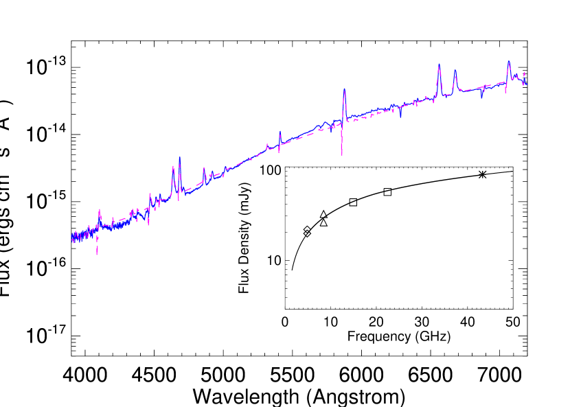
Figure 9: The observed GTC spectrum of the WN8 component in WR 147 (blue solid line) overlaid with the cmfgen model (magenta dashed line) using modified volume filling factor (see Fig. 11, right panel). The observed radio emission of the WN8 component (as in Fig. 8) and the corresponding theoretical spectrum are shown in the inset figure.

Figure 10: The characteristic radius of the radio emission of the WN8 component in WR 147 normalized to the binary separation ($D_{WR~{}147}$). The dashed line denotes the location of the colliding-wind zone.

4.3 Global physical picture

All this (Section 4.1, 4.2) shows that a global view on the colliding-wind binary WR 147 could be a reasonable approach for describing its observational characteristics in a consistent way. Namely, analysis of optical spectra with the help of grid-modelling, based on modern stellar atmosphere models (e.g., cmfgen), provides physical parameters of the massive stars which explain well not only the optical spectrum but the radio and X-ray emission from this colliding-wind binary. A basic ‘ingredient’ in the physical picture is the presence of non-homogeneous stellar winds as the volume filling factor of the clumps should decrease with distance from the massive star. And, there is an important consequence from the latter.

In a massive star, UV/optical emission forms relatively close to the star: at distance smaller than a few tens or a hundred stellar radii. Its radio-formation region extends to at least a few thousands stellar radii. And in wide massive binaries, there is strong X-ray emission that originates from the interaction zone of the stellar winds of the binary components, which could be located very far from the stars themselves. This is indeed the case for the CSW binary WR 147: the ratio of the characteristic radius of the radio emission of its WR component to binary separation is shown in Fig. 10. We see that the X-ray formation zone, that is the CSW zone, is located far beyond the radio-formation region.

Then, since the stellar winds of massive stars are clumpy (with rather small volume filling factor for the clumps; e.g. $f\leq 0.1$ in WR 147), how do clumps manage to collide and form the CSW zone? We recall that if CSW region does exist, then clumps are quickly heated up and dissolved in it after having crossed the shock fronts of the CSW zone (e.g., Pittard 2007). It thus seems reasonable to propose that stellar winds of massive stars are two-component flows: the more massive component consists of dense clumps that occupy a small fraction of the stellar wind volume, and there is a tenuous (low-density) component that fills in the rest of the volume. In such a physical picture, there is no problem for the low-density components of both massive stars in the binary to interact and set up the ‘seed’ CSW region. The more massive components of the stellar winds (the clumps) then interact with it and provide the strong X-ray emission observed from wide CSW binaries.

It is our understanding that the physical picture of massive stars possessing two-component stellar winds is capable of explaining observational characteristics of these objects along the entire spectral range. At least, this is the case with the CSW binary WR 147 for which such a physical picture describes its optical, radio and X-ray properties in a self-consistent way. We thus believe that by adopting the same global view on other CSW binaries we can further check the validity of this physical picture. An important task for future studies is to estimate the contribution of the low-density component of the stellar wind to the observed spectrum of a massive star: an issue that needs be addressed both from observational and theoretical point of view.

5 Conclusions

In this work, we presented an analysis of new optical spectra of WR 147 obtained with Gran Telescopio CANARIAS and of archive spectra from the Hubble Space Telescope. Our goal was to derive some basic parameters of both stellar components in order to check the global physical picture of this CSW binary. The basic results and conclusions from our analysis of these data are as follows.

(i) Given the spatial separation of 0$\aas@@fstack{\prime\prime}$64 between the stellar components in WR 147, individual optical spectra of its WR and OB components were extracted from the GTC spectra adopting a ‘deconvolution’ technique, while a standard aperture extraction was performed for the HST spectra.

(ii) The spectral modelling of the flux-calibrated WR and OB spectra is based on modern atmosphere models (cmfgen) that take into account the optically thin clumping (volume filling factor). We adopted a grid-modelling approach to derive some basic physical characteristics of the studied massive stars: e.g., the mass-loss rate ($\dot{M}$), luminosity (L), stellar temperature (T_∗). The spectral fits provided the optical extinction E(B-V) as well.

(iii) We note that for the currently accepted distance of 630 pc to WR 147, the values of mass-loss rate derived from modelling its optical spectra are in acceptable correspondence with that from modelling its X-ray emission: $\log~{}\dot{M}$ $=-4.95;-4.86$ (GTC; HST) vs. $\log~{}\dot{M}$ $=-5.0$  M_⊙ yr^-1 (Chandra; Zhekov & Park 2010b).

(iv) In the light of a global view on CSW binaries, we modelled the radio emission from WR 147 as well. It was done in two ways: directly with cmfgen and adopting the standard model for radio emission from massive stars (Panagia & Felli 1975; Wright & Barlow 1975). Correspondence between results from both models was very good, thus, showing that both can be used in analysis of radio emission from massive stars. However, the mass-loss rate, derived from modelling the optical spectra of WR 147, gives lower radio flux than observed. A plausible solution for this problem could be if the volume filling factor at large distance from the star (radio-formation region) is smaller than close to the star (optical-formation region). Adopting this, the model (cmfgen) can match well both optical and thermal radio emission from WR 147.

(v) The global view on the CSW binary WR 147 thus shows that its observational properties in different spectral domains can be explained in a self-consistent physical picture.

Appendix A Modified stellar wind clumping

Figure 11: The volume filling factor. Left panel: a schematic diagram illustrating the definition of the volume filling factor. Right panel: a comparison between the cases of the standard filling factor (CMFGEN) and that if clumps are allowed to expand.

Let us consider a simplified picture, that is a spherically-symmetric stellar wind is clumpy and the clumps are ‘identical’. So, the volume filling factor is defined as:

$$f=\frac{\frac{4\pi}{3}R_{cl}^{3}N_{cl}}{4\pi r^{2}2R_{cl}}=\frac{N_{cl}}{6}\left(\frac{R_{cl}}{r}\right)^{2}$$

where $f$ is the volume filling factor, $R_{cl}$ is the clump radius, $r$ is the distance from the star, $N_{cl}$ is the number of clumps (see Fig. 11, left panel).

Assuming that the clumps are quasi isothermal and they expand with the sound speed ($c_{s}$) determined by their plasma temperature, we have:

$$f=\frac{N_{cl}}{6}\left[\frac{R_{cl,0}+c_{s}(t-t_{0})}{r}\right]^{2}$$

where $R_{cl,0}$ is the clump radius at some initial (fiducial) time $t_{0}$, which corresponds to some initial (fiducial) distance $r_{0}$.

For a stellar wind with a constant velocity $\varv_{w}$, we have:

$$f=\frac{N_{cl}}{6}\left[\frac{R_{cl,0}+\frac{c_{s}}{\varv_{\infty}}(r-r_{0})}{r}\right]^{2},\hskip 28.45274ptf_{0}=\frac{N_{cl}}{6}\left(\frac{R_{cl,0}}{r_{0}}\right)^{2},$$

$$f_{\infty}=f_{0}\left(\frac{r_{0}}{R_{cl,0}}\right)^{2}\left(\frac{c_{s}}{\varv_{w}}\right)^{2}$$

where $f_{0}$ is the volume filling factor at radius $r_{0}$ and $f_{\infty}$ is the filling factor at large radius (infinity).

For a stellar wind with a $\beta$-law velocity ($\beta=1$), we have:

$$\varv=\varv_{0}+(\varv_{w}-\varv_{0})\left(1-\frac{r_{0}}{r}\right),\hskip 28.45274pt\varv=\varv_{w}\left[\alpha+(1-\alpha)\left(1-\frac{r_{0}}{r}\right)\right]$$

where $\varv_{0}$ is the wind velocity at radius $r_{0}$, $\varv_{\infty}$ is the terminal wind velocity and $\alpha=\varv_{0}/\varv_{w}$

So, we can write:

$$t-t_{0}=\int dt=\int\frac{dr}{\varv}=\frac{r_{0}}{\varv_{\infty}}\int\frac{d\tilde{r}}{\alpha+(1-\alpha)\left(1-\frac{1}{\tilde{r}}\right)}$$

as the distance $r$ is normalized to $r_{0}$, that is at time $t_{0}$ the distance is $\tilde{r}=1$ ($\tilde{r}=r/r_{0}$). After some manipulations we end up with:

$$t-t_{0}=\frac{r_{0}}{\varv_{\infty}}\left[(\tilde{r}-1)+(1-\alpha)\ln\frac{\tilde{r}-(1-\alpha)}{\alpha}\right]$$

And for the filling factor, we have:

$$f=f_{0}\left\{\frac{1+\frac{r_{0}}{R_{cl,0}}\frac{c_{s}}{\varv_{\infty}}\left[(\tilde{r}-1)+(1-\alpha)\ln\frac{\tilde{r}-(1-\alpha)}{\alpha}\right]}{\tilde{r}}\right\}^{2}$$

or

$$f=f_{0}\left\{\frac{1+\sqrt{\frac{f_{\infty}}{f_{0}}}\left[(\tilde{r}-1)+(1-\alpha)\ln\frac{\tilde{r}-(1-\alpha)}{\alpha}\right]}{\tilde{r}}\right\}^{2}$$

Note, the volume filling factor at large distances could be smaller or larger than its initial value, for example:

$$if\,\,\,f_{\infty}<f_{0}\hskip 5.69046pt\Longrightarrow\hskip 5.69046pt\left(\frac{r_{0}}{R_{cl,0}}\right)^{2}\left(\frac{c_{s}}{\varv_{w}}\right)^{2}<1\hskip 5.69046pt\Longrightarrow\hskip 5.69046pt\frac{R_{cl,0}}{r_{0}}>\frac{c_{s}}{\varv_{w}}$$

We could assume that clumps form at distances smaller than some ‘setup’ distance/radius ($r_{s}>r_{0}$), so, the filling factor has its standard cmfgen form (see eq. 1) in this inner region ($r<r_{s}$). And, beyond that clump-formation region ($r>r_{s}$) clumps may only expand but no new clumps appear. In such a case, the clump expansion will start at some initial time $t_{s}$ and similarly as above, we can derive:

$$f = f_{s}\left\{\frac{\tilde{r}_{s}+\sqrt{\frac{f_{\infty}}{f_{0}}}\left[(\tilde{r}-\tilde{r}_{s})+(1-\alpha)\ln\frac{\tilde{r}-(1-\alpha)}{\tilde{r}_{s}-(1-\alpha})\right]}{\tilde{r}}\right\}^{2}$$

$$f_{s} = \frac{N_{cl}}{6}\left(\frac{R_{cl,0}}{r_{s}}\right)^{2},\hskip 28.45274ptf_{\infty}=f_{s}\left(\frac{r_{s}}{R_{cl,0}}\right)^{2}\left(\frac{c_{s}}{\varv_{w}}\right)^{2}$$

We can also express the volume filling factor in terms of flow velocity with $\varv_{s}$ denoting its value at the clump-formation distance/radius $r_{s}$ ($\tilde{\varv}=\varv/\varv_{\infty}$):

$$f=\frac{f_{s}}{(1-\tilde{\varv}_{s})^{2}}\times$$

(4)

$$\left\{1-\tilde{\varv}+\sqrt{\frac{f_{\infty}}{f_{s}}}\left[\tilde{\varv}-\tilde{\varv}_{s}+(1-\tilde{\varv})(1-\tilde{\varv}_{s})\ln\left(\frac{\tilde{\varv}}{1-\tilde{\varv}}\frac{1-\tilde{\varv}_{s}}{\tilde{\varv}_{s}}\right)\right]\right\}^{2}$$

An example of how the filling factor changes if the clumps are allowed to expand is shown in Fig. 11 (right panel). The standard filling factor (CMFGEN; see eq. 1) is 0.1 while the case of expanding clumps has a value of $f_{\infty}=0.04$ at large radii from the star (where the wind reaches the terminal wind velocity). In this particular case, the clump-formation radius corresponds to $\tilde{\varv}_{s}\approx 0.2$.

Appendix B Model atoms used in cmfgen 

Adopted atomic data of all elements included in our model atmosphere calculations are summarized in Table 2. While the energy levels for HeI are from Martin (1987), most of the atomic data are from the Opacity (Seaton, 1987) and the Iron (Hummer et al., 1993) projects. However, for some CNO elements, atomic data were used also from Nussbaumer & Storey (1983, 1984), whilst for Iron data were used from Nahar (1995), Zhang (1996), Becker & Butler (1995a, b).

Table 2: Model atoms used in our models. For each ion the number of full levels, super levels, and bound-bound transitions is provided.

Ion	Super levels	Full levels	b-b transitions
H I	20	30	435
He I	45	69	907
He II	22	30	435
C II	10	18	47
C III	99	243	5528
C IV	59	64	1446
C V	46	73	490
N II	9	17	29
N III	41	82	582
N IV	200	278	6943
O II	81	182	2800
O III	165	343	6516
O IV	71	138	1597
Ne II	25	116	1732
Ne III	57	188	2343
Mg III	41	201	3052
Al III	7	12	26
Al IV	62	199	2992
Si III	26	51	245
Si IV	55	66	1090
Si V	52	203	3086
P IV	30	90	656
P V	9	15	42
S III	41	83	601
S IV	69	194	3598
S V	41	167	2229
Ar III	18	82	604
Ar IV	41	204	3459
Ca III	41	208	2784
Ca IV	39	341	7250
Fe IV	100	1000	37899
Fe V	45	869	31688
Fe VI	55	674	20240
Fe VII	13	50	237

References

- Abbott et al. (1981) Abbott D. C., Bieging J. H., Churchwell E., 1981, ApJ, 250, 645
- Abbott et al. (1986) Abbott D. C., Beiging J. H., Churchwell E., Torres A. V., 1986, ApJ, 303, 239
- Asplund et al. (2009) Asplund M., Grevesse N., Sauval A. J., Scott P., 2009, ARA&A, 47, 481
- Bailer-Jones et al. (2018) Bailer-Jones C. A. L., Rybizki J., Fouesneau M., Mantelet G., Andrae R., 2018, AJ, 156, 58
- Becker & Butler (1995a) Becker S. R., Butler K., 1995a, A&A, 294, 215
- Becker & Butler (1995b) Becker S. R., Butler K., 1995b, A&A, 301, 187
- Bessell & Murphy (2012) Bessell M., Murphy S., 2012, PASP, 124, 140
- Casagrande & VandenBerg (2014) Casagrande L., VandenBerg D. A., 2014, MNRAS, 444, 392
- Chambers et al. (2016) Chambers K. C., et al., 2016, arXiv e-prints, p. arXiv:1612.05560
- Cherepashchuk (1976) Cherepashchuk A. M., 1976, Soviet Astronomy Letters, 2, 138
- Churchwell et al. (1992) Churchwell E., Bieging J. H., van der Hucht K. A., Williams P. M., Spoelstra T. A. T., Abbott D. C., 1992, ApJ, 393, 329
- Contreras & Rodríguez (1999) Contreras M. E., Rodríguez L. F., 1999, ApJ, 515, 762
- Contreras et al. (1996) Contreras M. E., Rodriguez L. F., Gomez Y., Velazquez A., 1996, ApJ, 469, 329
- Dougherty & Williams (2000) Dougherty S. M., Williams P. M., 2000, MNRAS, 319, 1005
- Eenens & Williams (1994) Eenens P. R. J., Williams P. M., 1994, MNRAS, 269, 1082
- Evans et al. (2018) Evans D. W., et al., 2018, A&A, 616, A4
- Fitzpatrick (1999) Fitzpatrick E. L., 1999, PASP, 111, 63
- Gaia Collaboration et al. (2018) Gaia Collaboration et al., 2018, A&A, 616, A1
- Hamann et al. (1995) Hamann W. R., Koesterke L., Wessolowski U., 1995, A&A, 299, 151
- Hamann et al. (2006) Hamann W.-R., Gräfener G., Liermann A., 2006, A&A, 457, 1015
- Hamann et al. (2019) Hamann W. R., et al., 2019, A&A, 625, A57
- Hillier & Lanz (2001) Hillier D. J., Lanz T., 2001, in Ferland G., Savin D. W., eds, Astronomical Society of the Pacific Conference Series Vol. 247, Spectroscopic Challenges of Photoionized Plasmas. p. 343
- Hillier & Miller (1999) Hillier D. J., Miller D. L., 1999, ApJ, 519, 354
- Hummer et al. (1993) Hummer D. G., Berrington K. A., Eissner W., Pradhan A. K., Saraph H. E., Tully J. A., 1993, A&A, 279, 298
- Kochanek et al. (2017) Kochanek C. S., et al., 2017, PASP, 129, 104502
- Lebedev & Myasnikov (1990) Lebedev M. G., Myasnikov A. V., 1990, Fluid Dynamics, 25, 629
- Leitherer et al. (1997) Leitherer C., Chapman J. M., Koribalski B., 1997, ApJ, 481, 898
- Lépine et al. (2001) Lépine S., Wallace D., Shara M. M., Moffat A. F. J., Niemela V. S., 2001, AJ, 122, 3407
- Lucy (1974) Lucy L. B., 1974, AJ, 79, 745
- Luo et al. (1990) Luo D., McCray R., Mac Low M.-M., 1990, ApJ, 362, 267
- Martin (1987) Martin W. C., 1987, Phys. Rev. A, 36, 3575
- Moran et al. (1989) Moran J. P., Davis R. J., Bode M. F., Taylor A. R., Spencer R. E., Argue A. N., Irwin M. J., Shanklin J. D., 1989, Nature, 340, 449
- Morris et al. (2000) Morris P. W., van der Hucht K. A., Crowther P. A., Hillier D. J., Dessart L., Williams P. M., Willis A. J., 2000, A&A, 353, 624
- Myasnikov & Zhekov (1993) Myasnikov A. V., Zhekov S. A., 1993, MNRAS, 260, 221
- Nahar (1995) Nahar S. N., 1995, A&A, 293, 967
- Niemela et al. (1998) Niemela V. S., Shara M. M., Wallace D. J., Zurek D. R., Moffat A. F. J., 1998, AJ, 115, 2047
- Nussbaumer & Storey (1983) Nussbaumer H., Storey P. J., 1983, A&A, 126, 75
- Nussbaumer & Storey (1984) Nussbaumer H., Storey P. J., 1984, A&AS, 56, 293
- Panagia & Felli (1975) Panagia N., Felli M., 1975, A&A, 39, 1
- Parkin et al. (2014) Parkin E. R., Pittard J. M., Nazé Y., Blomme R., 2014, A&A, 570, A10
- Pittard (2007) Pittard J. M., 2007, ApJ, 660, L141
- Press et al. (1992) Press W. H., Teukolsky S. A., Vetterling W. T., Flannery B. P., 1992, Numerical recipes in FORTRAN. The art of scientific computing. Cambridge: University Press, |c1992, 2nd ed.
- Prilutskii & Usov (1976) Prilutskii O. F., Usov V. V., 1976, Soviet Ast., 20, 2
- Prinja & Crowther (1998) Prinja R. K., Crowther P. A., 1998, MNRAS, 300, 828
- Prinja et al. (1990) Prinja R. K., Barlow M. J., Howarth I. D., 1990, ApJ, 361, 607
- Rate & Crowther (2020) Rate G., Crowther P. A., 2020, MNRAS, arXiv:1912.10125,
- Richardson (1972) Richardson W. H., 1972, Journal of the Optical Society of America (1917-1983), 62, 55
- Sander et al. (2012) Sander A., Hamann W.-R., Todt H., 2012, A&A, 540, A144
- Schmidt-Kaler (1982) Schmidt-Kaler T., 1982, Bulletin d’Information du Centre de Donnees Stellaires, 23, 2
- Schmutz et al. (1989) Schmutz W., Hamann W. R., Wessolowski U., 1989, A&A, 210, 236
- Seaton (1987) Seaton M. J., 1987, Journal of Physics B Atomic Molecular Physics, 20, 6363
- Shappee et al. (2014) Shappee B. J., et al., 2014, ApJ, 788, 48
- Shepard (1968) Shepard D., 1968, in Proceedings of the 1968 23rd ACM National Conference. ACM ’68. ACM, New York, NY, USA, pp 517–524, doi:10.1145/800186.810616, http://doi.acm.org/10.1145/800186.810616
- Skinner et al. (1999) Skinner S. L., Itoh M., Nagase F., Zhekov S. A., 1999, ApJ, 524, 394
- Stevens et al. (1992) Stevens I. R., Blondin J. M., Pollock A. M. T., 1992, ApJ, 386, 265
- Tonry et al. (2012) Tonry J. L., et al., 2012, ApJ, 750, 99
- van der Hucht (2001) van der Hucht K. A., 2001, New Astron. Rev., 45, 135
- van der Hucht et al. (1986) van der Hucht K. A., Cassinelli J. P., Williams P. M., 1986, A&A, 168, 111
- Williams (1995) Williams P. M., 1995, in van der Hucht K. A., Williams P. M., eds, IAU Symposium Vol. 163, Wolf-Rayet Stars: Binaries; Colliding Winds; Evolution. p. 335
- Williams (2008) Williams P. M., 2008, in Revista Mexicana de Astronomia y Astrofisica Conference Series. pp 71–76
- Williams et al. (1997) Williams P. M., Dougherty S. M., Davis R. J., van der Hucht K. A., Bode M. F., Setia Gunawan D. Y. A., 1997, MNRAS, 289, 10
- Wright & Barlow (1975) Wright A. E., Barlow M. J., 1975, MNRAS, 170, 41
- Zel’dovich & Raizer (1967) Zel’dovich Y. B., Raizer Y. P., 1967, Physics of shock waves and high-temperature hydrodynamic phenomena. Dover Publications, Inc., New York
- Zhang (1996) Zhang H., 1996, A&AS, 119, 523
- Zhekov (2015) Zhekov S. A., 2015, MNRAS, 447, 2706
- Zhekov (2017) Zhekov S. A., 2017, MNRAS, 472, 4374
- Zhekov & Park (2010a) Zhekov S. A., Park S., 2010a, ApJ, 709, L119
- Zhekov & Park (2010b) Zhekov S. A., Park S., 2010b, ApJ, 721, 518