Inspector Gadget: A Data Programming-based Labeling System for Industrial Images

Abstract.

As machine learning for images becomes democratized in the Software 2.0 era, one of the serious bottlenecks is securing enough labeled data for training. This problem is especially critical in a manufacturing setting where smart factories rely on machine learning for product quality control by analyzing industrial images. Such images are typically large and may only need to be partially analyzed where only a small portion is problematic (e.g., identifying defects on a surface). Since manual labeling these images is expensive, weak supervision is an attractive alternative where the idea is to generate weak labels that are not perfect, but can be produced at scale. Data programming is a recent paradigm in this category where it uses human knowledge in the form of labeling functions and combines them into a generative model. Data programming has been successful in applications based on text or structured data and can also be applied to images usually if one can find a way to convert them into structured data. In this work, we expand the horizon of data programming by directly applying it to images without this conversion, which is a common scenario for industrial applications. We propose Inspector Gadget, an image labeling system that combines crowdsourcing, data augmentation, and data programming to produce weak labels at scale for image classification. We perform experiments on real industrial image datasets and show that Inspector Gadget obtains better performance than other weak-labeling techniques: Snuba, GOGGLES, and self-learning baselines using convolutional neural networks (CNNs) without pre-training.

1. Introduction

In the era of Software 2.0, machine learning techniques for images are becoming democratized where the applications range from manufacturing to medical. For example, smart factories regularly use computer vision techniques to classify defective and non-defective product images (Oztemel and Gursev, 2018). In medical applications, MRI scans are analyzed to identify diseases like cancer (Liu et al., 2018). However, many companies are still reluctant to adapt machine learning due to the lack of labeled data where manual labeling is simply too expensive (Stonebraker and Rezig, 2019).

We focus on the problem of scalable labeling for classification where large images are partially analyzed, and there are few or no labels to start with. Although many companies face this problem, it has not been studied enough. Based on a collaboration with a large manufacturing company, we provide the following running example. Suppose there is a smart factory application where product images are analyzed for quality control (Figure 1). These images taken from industrial cameras usually have high-resolution. The goal is to look at each image and tell if there are certain defects (e.g., identify scratches, bubbles, and stampings). For convenience, we hereafter use the term defect to mean a part of an image of interest.

Figure 1. Labeling industrial images with Inspector Gadget in a smart factory application.

A conventional solution is to collect enough labels manually and train say a convolutional neural network on the training data. However, fully relying on crowdsourcing for image labeling can be too expensive. In our application, we have heard of domain experts demanding six-figure salaries, which makes it infeasible to simply ask them to label images. In addition, relying on general crowdsourcing platforms like Amazon Mechanical Turk may not guarantee high-enough labeling quality.

Among the possible methods for data labeling (see an extensive survey (Roh et al., 2019)), weak supervision is an important branch of research where the idea is to semi-automatically generate labels that are not perfect like manual ones. Thus, these generated labels are called weak labels, but they have reasonable quality where the quantity compensates for the quality. Data programming (Ratner et al., 2016) is a representative weak supervision technique of employing humans to develop labeling functions (LFs) that individually perform labeling (e.g., identify a person riding a bike), perhaps not accurately. However, the combination of inaccurate LFs into a generative model results in probabilistic labels with reasonable quality. These weak labels can then be used to train an end discriminative model.

So far, data programming has been shown to be effective in finding various relationships in text and structured data (Ratner et al., 2017). Data programming has also been successfully applied to images where they are usually converted to structured data beforehand (Varma et al., 2017; Varma et al., 2019). However, this conversion limits the applicability of data programming. As an alternative approach, GOGGLES (Das et al., 2020) demonstrates that, on images, automatic approaches using pre-trained models may be more effective. Here the idea is to extract semantic prototypes of images using the pre-trained model and then cluster and label the images using the prototypes. However, GOGGLES also has limitations (see Section 6.2), and it is not clear if it is the only solution for generating training data for image classification.

We thus propose Inspector Gadget, which opens up a new class of problems for data programming by enabling direct image labeling at scale without the need to convert to structured data using a combination of crowdsourcing, data augmentation, and data programming techniques. Inspector Gadget provides a crowdsourcing workflow where workers identify patterns that indicate defects. Here we make the tasks easy enough for non-experts to contribute. These patterns are augmented using general adversarial networks (GANs) (Goodfellow et al., 2014) and policies (Cubuk et al., 2018). Each pattern effectively becomes a labeling function by being matched with other images. The similarities are then used as features to train a multi-layer perceptron (MLP), which generates weak labels.

In our experiments, Inspector Gadget performs better overall than state-of-the-art methods: Snuba, GOGGLES, and self-learning baselines that use CNNs (VGG-19 (Simonyan and Zisserman, 2015) and MobileNetV2 (Sandler et al., 2018)) without pre-training. We release our code as a community resource (git, [n.d.]).

In the rest of the paper, we present the following:

• The architecture of Inspector Gadget (Section 2).

• The component details of Inspector Gadget:

  • Crowdsourcing workflow for helping workers identify patterns (Section 3).

  • Pattern augmenter for expanding the patterns using GANs and policies (Section 4).

  • Feature generator and labeler for generating similarity features and producing weak labels (Section 5).

• Experimental results where Inspector Gadget outperforms other image labeling techniques – Snuba, GOGGLES, and self-learning baselines using CNNs – where there are few or no labels to start with (Section 6).

2. Overview

The main technical contribution of Inspector Gadget is its effective combination of crowdsourcing, data augmentation, and data programming for scalable image labeling for classification. Figure 2 shows the overall process of Inspector Gadget. First, a crowdsourcing workflow helps workers identify patterns of interest from images that may indicate defects. While the patterns are informative, they may not be enough and are thus augmented using generative adversarial networks (GANs) (Goodfellow et al., 2014) and policies (Cubuk et al., 2019). Each pattern effectively becomes a labeling function where it is compared with other images to produce similarities that indicate whether the images contain defects. A separate development set is used to train a small model that uses the similarity outputs as features. This model is then used to generate weak labels of images indicating the defect types in the test set. Figure 3 shows the architecture of the Inspector Gadget system. After training the Labeler, Inspector Gadget only utilizes the components highlighted in gray for generating weak labels. In the following sections, we describe each component in more detail.

Figure 2. An overview of how Inspector Gadget constructs a model (labeler) that generates weak labels.

Figure 3. The architecture of Inspector Gadget.

Figure 4. The crowdsourcing workflow of Inspector Gadget. Crowd workers can interact with a UI and provide bounding boxes that identify defects. The boxes are used as patterns, which are combined or go through a peer review phase.

3. Crowdsourcing Workflow

Since collecting enough labels on the entire images are too expensive, we would like to utilize human knowledge as much as possible and reduce the additional amount of labeled data. We propose a crowdsourcing workflow shown in Figure 4. First, the workers mark defects using bounding boxes through a UI. Since the workers are not necessarily experts, the UI educates them how to identify defects beforehand. The bounding boxes in turn become the patterns we use to find other defects. Figure 5 shows sample images of a real-world smart factory dataset (called Product; see Section 6.1 for a description) where defects are highlighted with red boxes. Notice that the defects are not easy to find as they are small and mixed with other parts of the product.

Figure 5. Sample images in the Product dataset (see Section 6.1) containing scratch, bubble, and stamping defects where we highlight each defect with a bounding box.

As with any crowdsourcing application, we may run into quality control issues where the bounding boxes of the workers vary even for the same defect. Inspector Gadget addresses this problem by first combining overlapping bounding boxes together. While there are several ways to combine boxes, we find that averaging their coordinates works reasonably well. The two other strategies we considered were to take the “union” of coordinates (i.e., find the coordinates that cover the overlapping boxes), or take the “intersection” of coordinates (i.e., find the coordinates for the common parts of the boxes). However, the union strategy tends to generate patterns that are too large, while the intersection strategy has the opposite problem of generating tiny patterns. Hence, we only use the average strategy in our experiments. For the remaining outlier boxes, Inspector Gadget goes through a peer review phase where workers discuss which ones really contain defects. In Section 6.3, we perform ablation tests to show how each of these steps helps improve the quality of patterns.

Another challenge is determining how many images must be annotated to generate enough patterns. In general, we may not have statistics on the portion of images that have defects. Hence, our solution is to randomly select images and annotate them until the number of defective images exceeds a given threshold. In our experiments, identifying tens of defective images is sufficient (see the $N_{V}^{D}$ values in Table 1). All the annotated images form a development set, which we use in later steps for training the labeler.

The crowdsourcing workflow can possibly be automated using pre-trained region proposal networks (RPNs) (Ren et al., 2015). However, this approach requires other training data with similar defects and bounding boxes, which seldom exist for our applications.

4. Pattern Augmenter

Pattern augmentation is a way to compensate for the possible lack of patterns even after using crowdsourcing. The patterns can be lacking if not enough human work is done to identify all possible patterns and especially if there are not enough images containing defects (i.e., there is a class imbalance) so one has to go through many images just to encounter a negative label. We would thus like to automatically generate more patterns without resorting to more expensive crowdsourcing.

We consider two types of augmentation – GAN-based (Goodfellow et al., 2014) and policy-based (Cubuk et al., 2018). The two methods complement each other and have been used together in medical applications for identifying lesions (Frid-Adar et al., 2018). GAN-based augmentation is good at generating random variations of existing defects that do not deviate significantly. On the other hand, policy-based augmentation is better for generating specific variations of defects that can be quite different, exploiting domain knowledge. In Section 6.4, we show that neither augmentation subsumes the other, and the two can be used together to produce the best results.

The augmentation can be done efficiently because we are augmenting small patterns instead of the entire images. For high-resolution images, it is sometimes infeasible to train a GAN at all. In addition, if most of the image is not of interest for analysis, it is difficult to generate fake parts of interest while leaving the rest of the image as is. By only focusing on augmenting small patterns, it becomes practical to apply sophisticated augmentation techniques.

4.1. GAN-based Augmentation

The first method is to use generative adversarial networks (GAN) to generate variations of patterns that are similar to the existing ones. Intuitively, these augmented patterns can fill in the gaps of the existing patterns. The original GAN (Goodfellow et al., 2014) trains a generator to produce realistic fake data where the goal is to deceive a discriminator that tries to distinguish the real and fake data. More recently, many variations have been proposed (see a recent survey (Wang et al., 2019)).

We use a Relativistic GAN (RGAN) (Jolicoeur-Martineau, 2019), which can efficiently generate more realistic patterns than the original GAN. The formulation of RGAN is:

$$\max_{D}\mathbb{E}_{(x_{r},G(z))\sim(\mathbb{P},\mathbb{Q})}[\mathrm{log}(\sigma(D(x_{r})-D(G(z))))]$$

$$\max_{G}\mathbb{E}_{(x_{r},G(z))\sim(\mathbb{P},\mathbb{Q})}[\mathrm{log}(\sigma(D(G(z))-D(x_{r})))]$$

where $G$ is the generator, $x_{r}$ is real data, $D(x)$ is the probability that $x$ is real, $z$ is a random noise vector that is used by $G$ to generate various fake data, and $\sigma$ is the sigmoid function. While training, the discriminator of RGAN not only distinguishes data, but also tries to maximize the difference between two probabilities: the probability that a real image is actually real, and the probability that a fake image is actually fake. This setup enforces fake images to be more realistic, in addition to simply being distinguishable from real images as in the original GAN. We also use Spectral Normalization (Miyato et al., 2018), which is a commonly-used technique applied to a neural network structure where the discriminator restricts the gradient to adjust the training speed for better training stability.

Another issue is that neural networks assume a fixed size and shape of its inputs. While this assumption is reasonable for a homogeneous set of images, the patterns may have different shapes. We thus fit patterns to a fixed-sized square shape by resizing them before augmentation. Then we re-adjust new patterns into one of the original sizes in order to properly find other defects. Figure 6 shows the entire process applied to an image. In Section 6.4, we show that the re-sizing of patterns is effective in practice.

Figure 6. GAN-based augmentation on a pattern containing a scratch defect from the Product dataset.

4.2. Policy-based Augmentation

Policies (Cubuk et al., 2018) have been proposed as another way to augment images and complement the GAN approach. The idea is to use manual policies to decide how exactly an image is varied. Figure 7 shows the results of applying four example policies on a surface defect from the KSDD dataset (see description in Section 6.1). Policy-based augmentation is effective for patterns where applying operations based on human knowledge may result in quite different, but valid patterns. For example, if a defect is line-shaped, then it makes sense to stretch or rotate it. There are two parameters to configure: the operation to use and the magnitude of applying that operation. Recently, policy-based techniques have become more automated, e.g., AutoAugment (Cubuk et al., 2018) uses reinforcement learning to decide to what extent can policies be applied together.

We use an simpler approach than AutoAugment. Among certain combinations of policies, we choose the ones that work best on the development set. We first split the development set into train and test sets. For each policy, we specify a range for the magnitudes and choose 10 random values within that range. We then iterate all combinations of three policies. For each combination, we augment the patterns in the train set using the 10 magnitudes and train a model (see details in Section 5) on the train set images until convergence. Then we evaluate the model on the separate test set. Finally, we use the policy combination that results in the best accuracy and apply it to the entire set of patterns.

Figure 7. Policy-based augmentation on a pattern with a crack defect from the KSDD dataset (see Section 6.1). For each augmentation, we show the operation and magnitude.

5. Weak Label Generation

Once Inspector Gadget gathers patterns and augments them, the next step is to generate features of images (also called primitives according to Snuba (Varma and Ré, 2018)) and train a model that can produce weak labels. Note that the way we generate features of images is more direct than existing data programming systems that first convert images to structured data with interpretable features using object detection (e.g., identify a vehicle) before applying labeling functions.

5.1. Feature Generator

Inspector Gadget provides feature generation functions (FGFs) that match all generated patterns with the new input image to identify similar defects on any location and return the similarities with the patterns. Notice that the output of an FGF is different than a conventional labeling function in data programming where the latter returns a weak label per image. A vector that consists of all output values of the FGFs on each image is used as the input of the labeler. Depending on the type of defect, the pattern matching may differ. A naïve approach is to do an exact pixel-by-pixel comparison, but this is unrealistic when the defects have variations. Instead, a better way is to compare the distributions of pixel values. This comparison is more robust to slight variations of a pattern. On the other hand, there may be false positives where an obviously different defect matches just because its pixels have similar distributions. In our experiments, we found that comparing distributions on the x and y axes using normalized cross correlation (ope, [n.d.]) is effective in reducing such false positives. Given an image $I$ with pixel dimensions $W\times H$ and pattern $P_{i}$ with dimensions $w\times h$, the $i^{th}$ FGF $f_{i}$ is defined as:

$${\color[rgb]{0,0,0}f_{i}(I)}=\max_{x,y}\left|\frac{\sum_{x^{\prime},y^{\prime}}P_{i}(x^{\prime},y^{\prime})\cdot I(x+x^{\prime},y+y^{\prime})}{\sqrt{\sum_{x^{\prime},y^{\prime}}P_{i}(x^{\prime},y^{\prime})^{2}\cdot{\color[rgb]{0,0,0}\sum_{x^{\prime},y^{\prime}}}I(x+x^{\prime},y+y^{\prime})^{2}}}\right|$$

where $0\leq x<W-w$, $0\leq y<H-h$, $0\leq x^{\prime}<w$, and $0\leq y^{\prime}<h$. When matching a pattern against an image, a straightforward approach is to make a comparison with every possible region of the same size in the image. However, scanning the entire image may be too time consuming. Instead, we use a pyramid method (Adelson et al., 1984) where we first search for candidate parts of an image by reducing the resolutions of the image and pattern and performing a comparison quickly. Then just for the candidates, we perform a comparison using the full resolution.

Table 1. For each of the five datasets, we show the image size, the dataset size($N$) and number of defective images($N^{D}$), the development set size($N_{V}$) and number of defective images within it($N_{V}^{D}$), the types of defects detected, and the task type.

Dataset	Image size	$N$ ($N^{D}$)	$N_{V}$ ($N_{V}^{D}$)	Defect Type	Task Type
KSDD (Tabernik et al., 2019)	500 x 1257	399 (52)	78 (10)	Crack	Binary
Product (scratch)	162 x 2702	1673 (727)	170 (76)	Scratch	Binary
Product (bubble)	77 x 1389	1048 (102)	104 (10)	Bubble	Binary
Product (stamping)	161 x 5278	1094 (148)	109 (15)	Stamping	Binary
NEU (He et al., 2020)	200 x 200	300 per defect	100 per defect	Rolled-in scale, Patches, Crazing,	Multi-class
				Pitted surface, Inclusion, Scratch

5.2. Labeler

After the features are generated, Inspector Gadget trains a model on the output similarities of the FGFs, where the goal is to produce weak labels. The model can have any architecture and be small because there are not as many features as say the number of pixels in an image. We use a multilayer perceptron (MLP) because it is simple, but also has good performance compared to other models. An interesting observation is that, depending on the model architecture (e.g., the number of layers in an MLP), the model accuracy can vary significantly as we demonstrate in Section 6.5. Inspector Gadget thus performs model tuning where it chooses the architecture that has the best accuracy results on the development set. This feature is powerful compared to existing CNN approaches where the architecture is complicated, and it is too expensive to consider other variations.

The labeling process after training the labeler consists of two steps. First, the patterns are matched to unlabeled images for generating the features. Second, the trained labeler is applied on the features to make a prediction for each unlabeled image. We note that latency is not the most critical issue because we are generating weak labels, which are used to construct the training data for the end discriminative model. Training data construction is usually done in batch mode instead of say real time.

6. Experiments

We evaluate Inspector Gadget on real datasets and answer the following questions.

• How accurate are the weak labels of Inspector Gadget compared to other labeling methods and are they useful when training the end discriminative model?

• How useful is each component of Inspector Gadget?

• What are the errors made by Inspector Gadget?

We implement Inspector Gadget in Python and use the OpenCV library and three machine learning libraries: Pytorch, TensorFlow, and Scikit-learn. We use an Intel Xeon CPU to train our MLP models and an NVidia Titan RTX GPU to train larger CNN models. Other details can be found in our released code (git, [n.d.]).

6.1. Settings

Datasets

We use real datasets for classification tasks. For each dataset, we construct a development set as described in Section 3. Table 1 summarizes the datasets with other experimental details, and Figures 5 and  8 shows samples of them. We note that the results in Section 6.2 are obtained by varying the size of the development set, and the rest of the experiments utilize the same size as described in Table 1. For each dataset, we have a gold standard of labels. Hence, we are able to compute the accuracy of the labeling on separate test data.

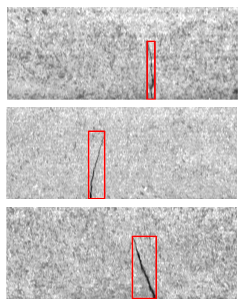
(a) KSDD data

(b) NEU data

Figure 8. Sample images in KSDD (Tabernik et al., 2019) and NEU (He et al., 2020) datasets where we highlight the defects with bounding boxes.

• The Kolektor Surface-Defect Dataset (KSDD (Tabernik et al., 2019)) is constructed from images of electrical commutators that were provided and annotated by the Kolektor Group. There is only one type of defect – cracks – but each one varies significantly in shape.

• The Product dataset (Figure 5) is proprietary and obtained through a collaboration with a manufacturing company. Each product has a circular shape where different strips are spread into rectangular shapes. There are three types of defects: scratches, bubbles, and stampings, which occur in different strips. The scratches vary in length and direction. The bubbles are more uniform, but have small sizes. The stampings are small and appear in fixed positions. We divide the dataset into three, as if there is a separate dataset for each defect type.

• The Northeastern University Surface Defect Database (NEU (He et al., 2020)) contains images that are divided into 6 defect types of surface defects of hot-rolled steel strips: rolled-in scale, patches, crazing, pitted surface, inclusion, and scratches. Compared to the other datasets, these defects take larger portions of the images. Since there are no images without defects, we solve the different task of multi-class classification where the goal is to determine which defect is present.

GAN-based Augmentation

We provide more details for Section 4.1. For all datasets, the input random noise vector has a size of 100, the learning rates of the generator and discriminator are both $1\mathrm{e}{-4}$, and the number of epochs is about 1K. We fit patterns to a square shape where the width and height are set to 100 or the averaged value of all widths and heights of patterns, whichever is smaller.

Labeler Tuning

We use an L-BFGS optimizer (Liu and Nocedal, 1989), which provides stable training on small data, with a $1\mathrm{e}{-5}$ learning rate. We use $k$-fold cross validation where each fold has at least 20 examples per class and early stopping in order to compare the accuracies of candidate models before they overfit.

Accuracy Measure

We use the $F_{1}$ score, which is the harmonic mean between precision and recall. Suppose that the set of true defects is $D$ while the set of predictions is $P$. Then the precision $Pr=\frac{|D\cap P|}{|P|}$, recall $Re=\frac{|D\cap P|}{|D|}$, and $F_{1}=\frac{2\times Pr\times Re}{Pr+Re}$. While there are other possible measures like ROC-AUC, $F_{1}$ is known to be more suitable for data where the labels are imbalanced (Gu and Zhu, 2009) as in most of our settings.

Systems Compared

We compare Inspector Gadget with other image labeling systems and self-learning baselines that train CNN models on available labeled data.

Snuba (Varma and Ré, 2018) automates the process of labeling function (LF) construction by starting from a set of primitives that are analogous to our FGFs and iteratively selecting subsets of them to train heuristic models, which becomes the LFs. Each iteration involves comparing models trained on all possible subsets of the primitives up to a certain size. Finally, the LFs are combined into a generative model. We faithfully implement Snuba and use our crowdsourced and augmented patterns for generating primitives, in order to be favorable to Snuba. However, adding more patterns quickly slows down Snuba as its runtime is exponential to the number of patterns.

We also compare with GOGGLES (Das et al., 2020), which takes the labeling approach of not using crowdsourcing. However, it relies on the fact that there is a pre-trained model and extracts semantic prototypes of images where each prototype represents the part of an image where the pre-trained model is activated the most. Each image is assumed to have one object, and GOGGLES clusters similar images for unsupervised learning. In our experiments, we use the opensourced code of GOGGLES.

Finally, we compare Inspector Gadget with self-learning (Triguero et al., 2015) baselines that train CNN models on the development set using cross validation and use them to label the rest of the images. Note that when we compare Inspector Gadget with a CNN model, we are mainly comparing their feature generation abilities. Inspector Gadget’s features are the pattern similarities while for VGG’s features are produced at the end of the convolutional layers. In both cases, the features go through a final fully-connected layer (i.e., MLP). To make a fair comparison, we experiment with both heavy and light-weight CNN models. For the heavy model, we use VGG-19 (Simonyan and Zisserman, 2015), which is widely used in the literature. For the light-weight model, we use MobileNetV2 (Sandler et al., 2018), which is designed to train efficiently in a mobile setting, but nearly has the performance of heavy CNNs. We also make a comparison with VGG-19 whose weights are pre-trained on ImageNet (Deng et al., 2009) and fine-tuned on each dataset. An alternative approach is to pre-train VGG-19 on other datasets in Table 1 instead of ImageNet. To see which approach is better, we compare the transfer learning results in Table 2. We observe that combining VGG-19 with ImageNet outperforms the other scenarios on all target datasets and thus use ImageNet to be favorable to transfer learning. In addition, we use preprocessing techniques on images that are favorable for the baselines. For example, the images from the Product dataset are long rectangles, so we split each image in half and stack them on top of each other to make them more square-like, which is advantageous for CNNs.

Table 2. Comparison of VGG-19 F1 scores when pre-trained on various datasets.

	Pre-trained on
Target	Product	Product	Product
Dataset	(scratch)	(bubble)	(stamping)	KSDD	ImageNet
Product (sc)	x	0.942	0.958	0.964	0.972
Product (bu)	0.535	x	0.531	0.453	0.913
Product (st)	0.798	0.810	x	0.781	0.900
KSDD	0.683	0.093	0.112	x	0.897

(a) Product (scratch)

(b) Product (bubble)

(c) Product (stamping)

(d) KSDD (Tabernik et al., 2019)

(e) NEU (He et al., 2020)

Figure 9. Weak label accuracy comparison between Inspector Gadget, Snuba (Varma and Ré, 2018), GOGGLES (Das et al., 2020), the self-learning baselines (SL) using VGG-19 (Simonyan and Zisserman, 2015) and MobileNetV2 (Sandler et al., 2018), and transfer learning baseline (TL) on different sizes of development set. Among the models that are not pre-trained, Inspector Gadget performs either the best or second-best in all figures.

6.2. Weak Label Accuracy

We compare the weak label accuracy of Inspector Gadget with the other methods by increasing the development set size and observing the $F_{1}$ scores in Figure 9. To clearly show how Inspector Gadget compares with other methods, we use a solid line to draw its plot while using dotted lines for the rest. Among the models that are not pre-trained (i.e., ignore “TL (VGG19 + Pre-training)” for now), we observe that Inspector Gadget performs best overall because it is either the best or second-best method in all figures. This result is important because industrial images have various defect types that must all be identified correctly. For KSDD (Figure 9(d)), Inspector Gadget performs the best because the pattern augmentation helps Inspector Gadget find more variations of cracks (see Section 6.4). For Product (Figures 9(a)–9(c)), Inspector Gadget consistently performs the first or second best despite the different characteristics of the defects. For NEU (Figure 9(e)), Inspector Gadget ranks first for the multi-class classification.

We explain the performances of other methods. Snuba consistently has a lower $F_{1}$ than Inspector Gadget possibly because the number of patterns is too large to handle. Instead of considering all combinations of patterns and training heuristic models, Inspector Gadget’s approach of training the labeler works better for our experiments. GOGGLES does not use gold labels for training and thus has a constant accuracy. In Figure 9(a), GOGGLES has a high $F_{1}$ because the defect sizes are large, and the pre-trained VGG-16 is effective in identifying them as objects. For the other figures, however, GOGGLES does not perform as well because the defect sizes are small and difficult to identify as objects. VGG-19 without pre-training (“SL (VGG19)”) only performs the best in Figure 9(c) where CNN models are very good at detecting stamping defects because they appear in a fixed location on the images. For other figures, VGG-19 performs poorly because there is not enough labeled data. MobileNetV2 does not perform well in any of the figures. Finally, the transfer learning method (“TL (VGG19 + Pre-training)”) shows a performance comparable to Inspector Gadget. In particular, transfer learning performs better in Figures 9(a), 9(c), and 9(e), while Inspector Gadget performs better in Figures 9(b) and 9(d) (for small dev. set sizes). While we do not claim that Inspector Gadget outperforms transfer learning models, it is thus an attractive option for certain types of defects (e.g., bubbles) and small dev. set sizes.

6.3. Crowdsourcing Workflow

We evaluate how effectively we can use the crowd to label and identify patterns using the Product datasets. Table 3 compares the full crowdsourcing workflow in Inspector Gadget with two variants: (1) a workflow that does not average the patterns at all and (2) a workflow that does average the patterns, but still does not perform peer reviews. We evaluate each scenario without using pattern augmentation. As a result, the full workflow clearly performs the best for the Product (scratch) and Product (stamping) datasets. For the Product (bubble) dataset, the workflow that does not combine patterns has a better average $F_{1}$, but the accuracies vary among different workers. Instead, it is better to use the stable full workflow without the variance.

Table 3. Crowdsourcing workflow ablation results

	$F_{1}$ scores
	No avg.	No	Full
Dataset	(${\pm std/2}$)	peer review	workflow
Product (scratch)	0.940 (${\pm 0.005}$)	0.952	0.960
Product (bubble)	0.616 (${\pm 0.045}$)	0.525	0.605
Product (stamping)	0.299 (${\pm 0.142}$)	0.543	0.595

Table 4. Pattern augmentation impact on Inspector Gadget. For each dataset, we highlight the highest $F_{1}$ score.

Dataset	No	Policy	GAN	Using
	Aug.	Based	Based	Both
KSDD (Tabernik et al., 2019)	0.415	0.578	0.509	0.688
Product (scratch)	0.958	0.965	0.962	0.979
Product (bubble)	0.617	0.702	0.715	0.701
Product (stamping)	0.700	0.700	0.765	0.859
NEU (He et al., 2020)	0.936	0.954	0.930	0.954

6.4. Pattern Augmentation

We evaluate how augmented patterns help improve the weak label $F_{1}$ score of Inspector Gadget. Table 4 shows the impact of the GAN-based and policy-based augmentation on the five datasets. Figure 10 shows how adding patterns impacts the $F_{1}$ score for the Product (bubble) dataset. While adding more patterns helps to a certain extent, it has diminishing returns afterwards. The results for the other datasets are similar, although sometimes noisier. The best number of augmented patterns differs per dataset, but falls in the range of 100–500. When using both methods, we simply combine the patterns from each augmentation. As a result, while each augmentation helps improve $F_{1}$, using both of them usually gives the best results. While adding more patterns thus helps to a certain extent, it does has diminishing returns afterwards.

Pattern augmentation is an important way to solve class imbalance where there are very few defects compared to non-defects. Among the five datasets, KSDD, Product (bubble), and Product (stamping) have relatively few numbers of defects, and they benefit the most from pattern augmentation where the performance lift compared to no augmentation ranges from 0.10–0.27.

Figure 10. Policy-based and GAN-based augmentation results on the Product (stamping) dataset.

6.5. Model Tuning

We evaluate the impact of model tuning on accuracy described in Section 5.2 as shown in Figure 11. We use an MLP with 1 to 3 hidden layers and varied the number of nodes per hidden layer to be one of {$2^{n}|n=1\ldots m\text{ and }2^{m-1}\leq I\leq 2^{m}$} where $I$ is the number of input nodes. For each dataset, we first obtain the maximum and minimum possible $F_{1}$ scores by evaluating all the tuned models we considered directly on the test data. Then, we compare these results with the (test data) $F_{1}$ score of the actual model that Inspector Gadget selected using the development set. We observe that the model tuning in Inspector Gadget can indeed improve the model accuracy, close to the maximum possible value.

Figure 11. The variations in $F_{1}$ scores when tuning the MLP model hyper-parameters.

6.6. End Model Accuracy

We now address the issue of whether the weak labels are actually helpful for training the end discriminative model. We compare the $F_{1}$ score of this end model with the same model that is trained on the development set. For the discriminative model, we use VGG-19 (Simonyan and Zisserman, 2015) for the binary classification tasks on KSDD and Product, and ResNet50 (He et al., 2016) for the multi-class task on NEU. We can use other discriminative models that have higher absolute $F_{1}$, but the point is to show the relative $F_{1}$ improvements when using weak labels. Table 5 shows that the $F_{1}$ scores improve by 0.02–0.36. In addition, the results of “Tip. Pnt” show that one needs to increase the sizes of the development sets by 1.874–7.565x for the discriminative models to obtain the same $F_{1}$ scores as Inspector Gadget.

Table 5. $F_{1}$ scores of end models trained on the development set (Dev. Set) only or the development set combined with the weak labels produced by Inspector Gadget (WL (IG)). Tip. Pnt shows how larger the development set must be for the Dev. Set approach to obtain the same $F_{1}$ score as WL (IG).

Dataset	End Model	Dev. Set	WL (IG)	Tip. Pnt
KSDD (Tabernik et al., 2019)	VGG19	0.499	0.700	$\times$3.248
Product (sc)	VGG19	0.925	0.978	$\times$4.374
Product (bu)	VGG19	0.359	0.720	$\times$6.041
Product (st)	VGG19	0.782	0.876	$\times$7.565
NEU (He et al., 2020)	ResNet50	0.953	0.970	$\times$1.874

6.7. Error Analysis

We perform an error analysis on which cases Inspector Gadget fails to make correct predicts for the five datasets based on manual investigation. We use the ground truth information for the analysis. Table 6 shows that most common error is when certain defects do not match with the patterns, which can be improved by using better pattern augmentation and matching techniques. The next common case is when the data is noisy, which can be improved by cleaning the data. The last case is the most challenging where even humans have difficulty identifying the defects because they are not obvious (e.g., a near-invisible scratch).

Table 6. Error analysis of Inspector Gadget.

	Cause
	Matching	Noisy	Difficult
Dataset	failure	data	to humans
KSDD (Tabernik et al., 2019)	10 (52.6 %)	5 (26.3 %)	4 (21.1 %)
Product (scratch)	11 (36.7 %)	11 (36.7 %)	8 (26.6 %)
Product (bubble)	19 (45.2 %)	15 (35.7 %)	8 (19.1 %)
Product (stamping)	15 (45.5 %)	13 (39.4 %)	5 (15.1 %)
NEU (He et al., 2020)	35 (63.6 %)	4 (7.3 %)	16 (29.1 %)

7. Related Work

Crowdsourcing for machine learning and databases

Using humans in advanced analytics is increasingly becoming mainstream (Xin et al., 2018) where the tasks include query processing (Marcus et al., 2011), entity matching (Gokhale et al., 2014), active learning (Mozafari et al., 2012), data labeling (Haas et al., 2015), and feature engineering (Cheng and Bernstein, 2015). Inspector Gadget provides a new use case where the crowd identifies patterns.

Data Programming

Data programming (Ratner et al., 2016) is a recent paradigm where workers program labeling functions (LFs), which are used to generate weak labels at scale. Snorkel (Ratner et al., 2017; Bach et al., 2019) is a seminal system that demonstrates the practicality of data programming, and Snuba (Varma and Ré, 2018) extends it by automatically constructing LFs using primitives. In comparison, Inspector Gadget does not assume any accuracy guarantees on the feature generation function and directly labels images without converting them to structured data.

Several systems have studied the problem of automating labeling function construction. CrowdGame (Liu et al., 2019) proposes a method for constructing LFs for entity resolution on structured data. Adversarial data programming (Pal and Balasubramanian, 2018) proposes a GAN-based framework for labeling with LF results and claims to be better than Snorkel-based approaches. In comparison, Inspector Gadget solves the different problem of partially analyzing large images.

Automatic Image labeling

There is a variety of general automatic image labeling techniques. Data augmentation (Shorten and Khoshgoftaar, 2019) is a general method to generate new labeled images. Generative adversarial networks (GANs) (Goodfellow et al., 2014) have been proposed to generate fake, but realistic images based on existing images. Policies (Cubuk et al., 2018) were proposed to apply custom transformations on images as long as they remain realistic. Most of the existing work operate on the entire images. In comparison, Inspector Gadget is efficient because it only needs to augment patterns, which are much smaller than the images. Label propagation techniques (Bui et al., 2018) organize images into a graph based on their similarities and then propagates existing labels of images to their most similar ones. In comparison, Inspector Gadget is designed for images where only a small part of them are of interest while the main part may be nearly identical to other images, so we cannot utilize the similar method. There are also application-specific defect detection methods (Song and Yan, 2013; He et al., 2020, 2019), some of which are designed for the datasets we used. In comparison, Inspector Gadget provides a general framework for image labeling. Recently, GOGGLES (Das et al., 2020) is an image labeling system that relies on a pre-trained model to extract semantic prototypes of images. In comparison, Inspector Gadget does not rely on pre-trained models and is more suitable for partially analyzing large images using human knowledge. Lastly, an interesting line of work is novel class detection (Scheirer et al., 2012) where the goal is to identify unknown defects. While Inspector Gadget assumes a fixed set of defects, it can be extended with these techniques.

8. Conclusion

We proposed Inspector Gadget, a scalable image labeling system for classification problems that effectively combines crowdsourcing, data augmentation, and data programming techniques. Inspector Gadget targets applications in manufacturing where large industrial images are partially analyzed, and there are few or no labels to start with. Unlike existing data programming approaches that convert images to structured data beforehand using object detection models, Inspector Gadget directly labels images by providing a crowdsourcing workflow to leverage human knowledge for identifying patterns of interest. The patterns are then augmented and matched with other images to generate similarity features for MLP model training. Our experiments show that Inspector Gadget outperforms other image labeling methods (Snuba, GOGGLES) and self-learning baselines using CNNs without pre-training. We thus believe that Inspector Gadget opens up a new class of problems to apply data programming.

9. Acknowledgments

This work was supported by a Google AI Focused Research Award, by SK Telecom, and by the Engineering Research Center Program through the National Research Foundation of Korea (NRF) funded by the Korean Government MSIT (NRF-2018R1A5A1059921).

References

- (1)
- git ([n.d.]) [n.d.]. Inspector Gadget Github repository. https://github.com/geonheo/InspectorGadget. Accessed July 15th, 2020.
- ope ([n.d.]) [n.d.]. OpenCV. https://docs.opencv.org/2.4/modules/imgproc/doc/object_detection.html. Accessed July 15th, 2020.
- Adelson et al. (1984) E. H. Adelson, C. H. Anderson, J. R. Bergen, P. J. Burt, and J. M. Ogden. 1984. 1984, Pyramid methods in image processing. RCA Engineer 29, 6 (1984), 33–41.
- Bach et al. (2019) Stephen H. Bach, Daniel Rodriguez, Yintao Liu, Chong Luo, Haidong Shao, Cassandra Xia, Souvik Sen, Alexander Ratner, Braden Hancock, Houman Alborzi, Rahul Kuchhal, Christopher Ré, and Rob Malkin. 2019. Snorkel DryBell: A Case Study in Deploying Weak Supervision at Industrial Scale. In SIGMOD. 362–375.
- Bui et al. (2018) Thang D. Bui, Sujith Ravi, and Vivek Ramavajjala. 2018. Neural Graph Learning: Training Neural Networks Using Graphs. In WSDM. 64–71.
- Cheng and Bernstein (2015) Justin Cheng and Michael S. Bernstein. 2015. Flock: Hybrid Crowd-Machine Learning Classifiers. In CSCW. 600–611.
- Cubuk et al. (2018) Ekin Dogus Cubuk, Barret Zoph, Dandelion Mané, Vijay Vasudevan, and Quoc V. Le. 2018. AutoAugment: Learning Augmentation Policies from Data. CoRR abs/1805.09501 (2018). arXiv:1805.09501
- Cubuk et al. (2019) Ekin D. Cubuk, Barret Zoph, Dandelion Mane, Vijay Vasudevan, and Quoc V. Le. 2019. AutoAugment: Learning Augmentation Strategies From Data. In CVPR. 113–123.
- Das et al. (2020) Nilaksh Das, Sanya Chaba, Sakshi Gandhi, Duen Horng Chau, and Xu Chu. 2020. GOGGLES: Automatic Training Data Generation with Affinity Coding. In SIGMOD.
- Deng et al. (2009) Jia Deng, Wei Dong, Richard Socher, Li-Jia Li, Kai Li, and Fei-Fei Li. 2009. ImageNet: A large-scale hierarchical image database. In CVPR. 248–255.
- Frid-Adar et al. (2018) Maayan Frid-Adar, Idit Diamant, Eyal Klang, Michal Amitai, Jacob Goldberger, and Hayit Greenspan. 2018. GAN-based synthetic medical image augmentation for increased CNN performance in liver lesion classification. Neurocomputing 321 (2018), 321–331.
- Gokhale et al. (2014) Chaitanya Gokhale, Sanjib Das, AnHai Doan, Jeffrey F Naughton, Narasimhan Rampalli, Jude Shavlik, and Xiaojin Zhu. 2014. Corleone: hands-off crowdsourcing for entity matching. In SIGMOD. 601–612.
- Goodfellow et al. (2014) Ian J. Goodfellow, Jean Pouget-Abadie, Mehdi Mirza, Bing Xu, David Warde-Farley, Sherjil Ozair, Aaron C. Courville, and Yoshua Bengio. 2014. Generative Adversarial Nets. In NIPS. 2672–2680.
- Gu and Zhu (2009) Qiong Gu and Zhihua Zhu, Liand Cai. 2009. Evaluation Measures of the Classification Performance of Imbalanced Data Sets. In CIIS, Zhihua Cai, Zhenhua Li, Zhuo Kang, and Yong Liu (Eds.). Berlin, Heidelberg, 461–471.
- Haas et al. (2015) Daniel Haas, Jiannan Wang, Eugene Wu, and Michael J Franklin. 2015. Clamshell: Speeding up crowds for low-latency data labeling. arXiv preprint arXiv:1509.05969 (2015).
- He et al. (2016) Kaiming He, Xiangyu Zhang, Shaoqing Ren, and Jian Sun. 2016. Deep Residual Learning for Image Recognition. In 2016 IEEE Conference on Computer Vision and Pattern Recognition, CVPR 2016, Las Vegas, NV, USA, June 27-30, 2016. IEEE Computer Society, 770–778.
- He et al. (2019) Y. He, K. Song, H. Dong, and Y. Yan. 2019. Semi-supervised defect classification of steel surface based on multi-training and generative adversarial network. Optics and Lasers in Engineering 122 (2019), 294–302.
- He et al. (2020) Yu He, Ke-Chen Song, Qinggang Meng, and Yunhui Yan. 2020. An End-to-end Steel Surface Defect Detection Approach via Fusing Multiple Hierarchical Features. IEEE Transactions on Instrumentation and Measurement 69 (04 2020), 1493–1504.
- Jolicoeur-Martineau (2019) Alexia Jolicoeur-Martineau. 2019. The relativistic discriminator: a key element missing from standard GAN. In ICLR.
- Liu and Nocedal (1989) Dong C. Liu and Jorge Nocedal. 1989. On the limited memory BFGS method for large scale optimization. Math. Program. 45, 1-3 (1989), 503–528.
- Liu et al. (2019) Tongyu Liu, Jingru Yang, Ju Fan, Zhewei Wei, Guoliang Li, and Xiaoyong Du. 2019. CrowdGame: A Game-Based Crowdsourcing System for Cost-Effective Data Labeling. In SIGMOD. 1957–1960.
- Liu et al. (2018) Yun Liu, Timo Kohlberger, Mohammad Norouzi, George Dahl, Jenny Smith, Arash Mohtashamian, Niels Olson, Lily Peng, Jason Hipp, and Martin Stumpe. 2018. Artificial Intelligence Based Breast Cancer Nodal Metastasis Detection: Insights into the Black Box for Pathologists. Archives of Pathology & Laboratory Medicine (2018).
- Marcus et al. (2011) Adam Marcus, Eugene Wu, David R Karger, Samuel Madden, and Robert C Miller. 2011. Crowdsourced databases: Query processing with people. Cidr.
- Miyato et al. (2018) Takeru Miyato, Toshiki Kataoka, Masanori Koyama, and Yuichi Yoshida. 2018. Spectral Normalization for Generative Adversarial Networks. CoRR abs/1802.05957 (2018). arXiv:1802.05957 http://arxiv.org/abs/1802.05957
- Mozafari et al. (2012) Barzan Mozafari, Purnamrita Sarkar, Michael J Franklin, Michael I Jordan, and Samuel Madden. 2012. Active learning for crowd-sourced databases. arXiv preprint arXiv:1209.3686 (2012).
- Oztemel and Gursev (2018) Ercan Oztemel and Samet Gursev. 2018. Literature review of Industry 4.0 and related technologies. Journal of Intelligent Manufacturing (2018).
- Pal and Balasubramanian (2018) Arghya Pal and Vineeth N. Balasubramanian. 2018. Adversarial Data Programming: Using GANs to Relax the Bottleneck of Curated Labeled Data. In CVPR. 1556–1565.
- Ratner et al. (2017) Alexander J. Ratner, Stephen H. Bach, Henry R. Ehrenberg, and Chris Ré. 2017. Snorkel: Fast Training Set Generation for Information Extraction. In SIGMOD (Chicago, Illinois, USA). 1683–1686.
- Ratner et al. (2016) Alexander J. Ratner, Christopher De Sa, Sen Wu, Daniel Selsam, and Christopher Ré. 2016. Data Programming: Creating Large Training Sets, Quickly. In NIPS. 3567–3575.
- Ren et al. (2015) Shaoqing Ren, Kaiming He, Ross Girshick, and Jian Sun. 2015. Faster r-cnn: Towards real-time object detection with region proposal networks. In Advances in neural information processing systems. 91–99.
- Roh et al. (2019) Yuji Roh, Geon Heo, and Steven Euijong Whang. 2019. A Survey on Data Collection for Machine Learning: a Big Data - AI Integration Perspective. IEEE TKDE (2019).
- Sandler et al. (2018) Mark Sandler, Andrew G. Howard, Menglong Zhu, Andrey Zhmoginov, and Liang-Chieh Chen. 2018. MobileNetV2: Inverted Residuals and Linear Bottlenecks. In CVPR. 4510–4520.
- Scheirer et al. (2012) Walter J Scheirer, Anderson de Rezende Rocha, Archana Sapkota, and Terrance E Boult. 2012. Toward open set recognition. IEEE transactions on pattern analysis and machine intelligence 35, 7 (2012), 1757–1772.
- Shorten and Khoshgoftaar (2019) Connor Shorten and Taghi M. Khoshgoftaar. 2019. A survey on Image Data Augmentation for Deep Learning. J. Big Data 6 (2019), 60.
- Simonyan and Zisserman (2015) Karen Simonyan and Andrew Zisserman. 2015. Very Deep Convolutional Networks for Large-Scale Image Recognition. In ICLR.
- Song and Yan (2013) Ke-Chen Song and Yunhui Yan. 2013. A noise robust method based on completed local binary patterns for hot-rolled steel strip surface defects. Applied Surface Science 285 (2013), 858–864.
- Stonebraker and Rezig (2019) Michael Stonebraker and El Kindi Rezig. 2019. Machine Learning and Big Data: What is Important? IEEE Data Eng. Bull. (2019).
- Tabernik et al. (2019) Domen Tabernik, Samo Šela, Jure Skvarč, and Danijel Skočaj. 2019. Segmentation-Based Deep-Learning Approach for Surface-Defect Detection. Journal of Intelligent Manufacturing (15 May 2019).
- Triguero et al. (2015) Isaac Triguero, Salvador García, and Francisco Herrera. 2015. Self-labeled techniques for semi-supervised learning: taxonomy, software and empirical study. Knowl. Inf. Syst. 42, 2 (2015), 245–284.
- Varma et al. (2017) Paroma Varma, Bryan D. He, Payal Bajaj, Nishith Khandwala, Imon Banerjee, Daniel L. Rubin, and Christopher Ré. 2017. Inferring Generative Model Structure with Static Analysis. In NeurIPS. 240–250.
- Varma and Ré (2018) Paroma Varma and Christopher Ré. 2018. Snuba: Automating Weak Supervision to Label Training Data. PVLDB 12, 3 (2018), 223–236.
- Varma et al. (2019) Paroma Varma, Frederic Sala, Ann He, Alexander Ratner, and Christopher Ré. 2019. Learning Dependency Structures for Weak Supervision Models. In ICML, Kamalika Chaudhuri and Ruslan Salakhutdinov (Eds.), Vol. 97. 6418–6427.
- Wang et al. (2019) Zhengwei Wang, Qi She, and Tomas E. Ward. 2019. Generative Adversarial Networks: A Survey and Taxonomy. CoRR abs/1906.01529 (2019). arXiv:1906.01529
- Xin et al. (2018) Doris Xin, Litian Ma, Jialin Liu, Stephen Macke, Shuchen Song, and Aditya G. Parameswaran. 2018. Accelerating Human-in-the-loop Machine Learning: Challenges and Opportunities. In DEEM@SIGMOD. 9:1–9:4.