Superradiance and stability of the novel 4D charged Einstein-Gauss-Bonnet black hole

Abstract

We investigated the superradiance and stability of the novel 4D charged Einstein-Gauss-Bonnet black hole which is recently inspired by Glavan and Lin [Phys. Rev. Lett. 124, 081301 (2020)]. We found that the positive Gauss-Bonnet coupling consant $\alpha$ enhances the superradiance, while the negative $\alpha$ suppresses it. The condition for superradiant instability is proved. We also worked out the quasinormal modes (QNMs) of the charged Einstein-Gauss-Bonnet black hole and found that the real part of all the QNMs live beyond the superradiance condition and the imaginary parts are all negative. Therefore this black hole is stable. When $\alpha$ makes the black hole extremal, there are normal modes.

1.Department of Physics and Siyuan Laboratory, Jinan University, Guangzhou 510632, China
2.Institute for Theoretical Physics and Cosmology, Zhejiang University of Technology, Hangzhou 310023, China
3.United Center for Gravitational Wave Physics, Zhejiang University of Technology, Hangzhou 310032, China
4. Center for High Energy Physics, Peking University, No.5 Yiheyuan Rd, Beijing 100871, P. R. China
5. Department of Physics and State Key Laboratory of Nuclear Physics and Technology, Peking University, No.5 Yiheyuan Rd, Beijing 100871, P.R. China

Email: zhangcy@email.jnu.edu.cn,   sjzhang84@hotmail.com,    lipch2019@pku.edu.cn,   minyongguo@pku.edu.cn.
      ^∗Corresponding author

1 Introduction

As elementary particles, black holes play a central role in gravity including the general relativity and other modified theories of gravity. Numerous studies of past have proven that black holes enjoy many extremely nontrivial effects. One of the most interesting effects is the Penrose progress, which is found to be a new mechanism that energy can be extracted from the Kerr black hole [1]. The most essential reason is the existence of ergoregions, where timelike particles can have negative energies. And superradiant effects soon entered people’s view as the wave counterpart of the Penross progress [2]. Penrose progress and superradiance both require dissipations which can be provided by the ergoregion for an uncharged, stationary and axisymmetric spacetime. But unlike Penrose progress, superradiance can also occur in a nonrotating charged black hole geometry [3, 4], which is fundamentally different from the first situation. Since a spacetime containing a nonrotating charged black hole is believed to be a effectively dissipative environment for charged fields.

Along this line of superradiance, lots of studies have been investigated in many aspects. On the side of a nonrotating charged black hole, superradiance from RN black holes has been done in [5] at linearized level by considering a charged scalar field propagating on a RN background with the help of frequency-domain method. The time-domain method was applied to extract amplification factors in [6]. Also, an analytical treatment was proposed to calculate the amplification factors when the frequency is small [7]. These results agree well and support the existence of superradiation in RN black hole geometry mutually. Furthermore, some other investigations including superradiance in nonasymptotically flat spacetimes, analogue black hole geometries or higher dimensional spacetimes, superradiance beyond GR have attracted a lot of attention as well. One is suggested to refer to the comprehensive review [5] to overlook the whole picture. Therein, superradiance from black holes in alternative theories of gravity has been studied only in a few cases [8]. Whether superradiance can be stronger in modified theories of gravity still remains a open question [5].

As we know, the Einstein-Gauss-Bonnet (EGB) gravity is accounted as one of the most promising candidates for modified gravity [9]. And recently, a novel 4D EGB gravity was proposed in [10], where the authors rescale the Gauss-Bonnet coupling constant $\alpha\to\alpha/(D-4)$ in the limit $D\to 4$ and found the corresponding static black hole solution, see also [11]. This new finding has stimulated a lot of attentions on many fronts [12, 13, 14, 15, 16, 17, 18, 19, 20, 21, 22, 23, 24, 25, 26, 27, 28, 29, 30, 31].

In this paper, we will explore the superradiance and stability of the novel 4D charged Einstein-Gauss-Bonnet black hole geometry [14]. Firstly, we determined the constraints on $\alpha$ and the charge of the black hole $Q$ maintaining the event horizon. Then, by considering a charged massless scalar perturbation of the background we obtain the amplification factor of the superradiance and give a detailed analysis of the effects of $\alpha$ under different other parameters. We also pay attention on stability. We use the asymptotic iteration method (AIM) [32] to solve the quasinormal modes (QNMs) of the charged scalar perturbation numerically by considering the system as a scattering process. We find there’s no instability for the charged 4D EGB black hole under perturbations no matter $\alpha$ is positive or negative in the corresponding allowed region. And very interestingly, we find normal modes are survived for the extremal black hole which is worthy of further studies.

The paper is organized as follows. In section 2, we shortly revisit the novel 4D EGB gravity and determine the constraints on the GB coupling constant and the charge of the black hole to insure the spacetime contains a static charged black hole. In section 3, we discuss the scalar field perturbation. And we move to the amplification in section 4. The stabily of the novel 4D charged EGB black hole is investigated in section 5. We summarize our conclusions in section 6.

2 The spherically symmetric 4D Charged EGB black hole

The action of the EGB gravity with electromagnetic field in $D$-dimensional spacetime has the form

$$S=\frac{1}{16\pi}\int d^{D}x\sqrt{-g}\left[R+\frac{\alpha}{D-4}\mathcal{G}^{2}-F_{\mu\nu}F^{\mu\nu}\right].$$ (2.1)

Here we have rescaled the coupling constant $\alpha$ by a factor $\frac{1}{D-4}$. The Gauss-Bonnet term reads

$$\mathcal{G}^{2}=R^{2}-4R_{\mu\nu}R^{\mu\nu}+R_{\mu\nu\alpha\beta}R^{\mu\nu\alpha\beta}=\frac{1}{4}\delta_{\rho\sigma\gamma\delta}^{\mu\nu\alpha\beta}R_{\ \ \mu\nu}^{\rho\sigma}R_{\ \ \alpha\beta}^{\gamma\delta}.$$ (2.2)

The Maxwell tensor $F_{\mu\nu}=\partial_{\mu}A_{\nu}-\partial_{\nu}A_{\mu}$, in which $A_{\mu}$ is the gauge potential. Varying the action with respect to the metric, one gets the equation of motion

$$G_{\mu\nu}+\frac{\alpha}{D-4}H_{\mu\nu}=T_{\mu\nu}.$$ (2.3)

Here $G_{\mu\nu}$ is the Einstein tensor and

$$H_{\mu\nu}=2(RR_{\mu\nu}-2R_{\mu\sigma}R_{\ \nu}^{\sigma}-2R_{\mu\sigma\nu\rho}R^{\sigma\rho}-R_{\mu\sigma\rho\beta}R_{\ \ \ \nu}^{\sigma\rho\beta})-\frac{1}{2}g_{\mu\nu}\mathcal{G}^{2}.$$ (2.4)

The energy-momentum tensor of the Maxwell field takes in this form

$$T_{\mu\nu}=\frac{1}{4}\left(F_{\mu\sigma}F_{\ \nu}^{\sigma}-\frac{1}{4}g_{\mu\nu}F_{\alpha\beta}F^{\alpha\beta}\right).$$ (2.5)

The term $H_{\mu\nu}$ comes from the variation of the Gauss-Bonet term, which is a topological invariant term in four dimension. Therefore it does not contribute to the dynamics in four dimension in general. It can be checked that $H_{\mu\nu}$ always contains a factor $D-4$ and thus disappears when $D=4$. However, by rescaling the coupling constant $\alpha$, the factor $D-4$ is canceled in (2.3). Then the Gauss-Bonnet term gives rise to non-trivial dynamics and novel black hole solutions were discover recently [10, 14].

The spherically symmetric charged black hole solution of (2.3) in four dimension has the form

$$ds^{2}=-f(r)dt^{2}+\frac{1}{f(r)}dr^{2}+r^{2}(d\theta^{2}+\sin^{2}\theta d\phi^{2}),$$ (2.6)

where

$$f(r)=1+\frac{r^{2}}{2\alpha}\left(1\pm\sqrt{1+4\alpha\left(\frac{2M}{r^{3}}-\frac{Q^{2}}{r^{4}}\right)}\right)$$ (2.7)

The gauge potential is

$$A=-\frac{Q}{r}dt.$$ (2.8)

Here $M$ is the black hole mass parameter, $Q$ is the charge of the black hole. In the vanishing limit of $\alpha$ and in the far region, only the negative branch recovers the Reissner-Nordström (RN) black hole. Thus we will only study the negative branch in this paper.

The solution has at most two horizons in appropriate parameter region,

$$r_{\pm}=M\pm\sqrt{M^{2}-Q^{2}-\alpha}.$$ (2.9)

We see that $Q$ can be greater than $M$ when $\alpha$ is negative. However, $\alpha$ can not be too negative. It must be ensured that the metric function is well defined when $r>r_{+}$. We show the allowed parameter region in Fig. 1. Hereafter, we fix $M=1$ for convenience. In region $A$, there is only one horizon $r_{+}$. In region $B$, there are two horizons $r_{\pm}$. The allowed region for $\alpha$ is

$$\begin{cases}Q^{2}-4-2\sqrt{4-2Q^{2}}<\alpha<1-Q^{2},&\text{when }0<Q<\sqrt{3/2},\\ Q^{2}-4-2\sqrt{4-2Q^{2}}<\alpha<Q^{2}-4+2\sqrt{4-2Q^{2}},&\text{when }\sqrt{3/2}<Q<\sqrt{2}.\end{cases}$$ (2.10)

Note that when $Q>1$, the solution has no RN black hole limit since $\alpha$ cannot tend to $0$ now.

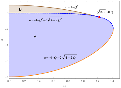
Figure 1: The parameter region where allows the event horizon $r_{+}$. Here we have fixed $M=1$. Region $B$ corresponds to $Q^{2}-4-2\sqrt{4-2Q^{2}}<\alpha<1-Q^{2}$ and $0<Q<\sqrt{3/2}$. Region $A$ corresponds to $Q^{2}-4-2\sqrt{4-2Q^{2}}<\alpha<Q^{2}-4+2\sqrt{4-2Q^{2}}$ and $0<Q<\sqrt{2}$.

3 The charged scalar perturbation

We consider a charged massless scalar perturbation of the background (2.6). It is known that fluctuations of order $\mathcal{O}(\epsilon)$ in the scalar field in a given background induce changes in the spacetime geometry of order $\mathcal{O}(\epsilon^{2})$ [5]. Therefore to leading order we can study the perturbations on a fixed background geometry. The massless charged scalar field $\psi$ has the perturbation equation as

$$0= D^{\mu}D_{\mu}\psi=g^{\mu\nu}\left(\nabla_{\mu}-iqA_{\mu}\right)\left(\nabla_{\nu}-iqA_{\nu}\right)\psi.$$ (3.1)

In spherically symmetric background, one can decompose the scalar field function as

$$\psi=\sum_{lm}\int d\omega e^{-i\omega t}\Psi(r)Y_{lm}(\theta,\phi).$$ (3.2)

Here $Y_{lm}(\theta,\phi)$ is the spherical harmonics on the two sphere $S^{2}.$ What we are interested in is the radial part of the equation.

$$0=\frac{1}{r^{2}}\partial_{r}\left(r^{2}f\partial_{r}\Psi\right)+\left(\frac{1}{f}\left(\omega-\frac{qQ}{r}\right)^{2}-\frac{l(l+1)}{r^{2}}\right)\Psi.$$ (3.3)

By introducing the tortoise coordinate $r_{\ast}$ and a new variable $\Psi_{0}$ as

$$dr=fdr_{\ast},\ \Psi=\frac{\Psi_{0}(r)}{r},$$ (3.4)

the radial equation can be written as the Schrödinger-like form

$$0=\frac{\partial^{2}\Psi_{0}}{\partial r_{\ast}^{2}}+\left(\left(\omega-\frac{qQ}{r}\right)^{2}-V_{\text{eff}}\right)\Psi_{0},$$ (3.5)

where the effective potential reads

$$V_{\text{eff}}=f\left(\frac{l(l+1)}{r^{2}}+\frac{\partial_{r}f}{r}\right).$$ (3.6)

The tortoise coordinate $r_{\ast}$ ranges from $-\infty$ to $\infty$ as $r$ runs from the event horizon $r_{+}$ to infinity. The effective potential vanishes as $r_{\ast}\to\pm\infty$ and has a potential barrier in the intermediate region. The asymptotic solution of (3.5) can be worked out as

$$\Psi_{0}\to \begin{cases}\mathcal{T}e^{-i\left(\omega-\frac{qQ}{r_{+}}\right)r_{\ast}},&r\to r_{+},\\ \mathcal{R}e^{i\omega r_{\ast}}+\mathcal{I}e^{-i\omega r_{\ast}},&r\to\infty,\end{cases}$$ (3.7)

where $\mathcal{I}$ corresponds to the incident amplitude at the infinity, $\mathcal{T},\mathcal{R}$ are the reflected and transmitted amplitudes, respectively. Thus we take this problem as a scattering process. Note that there is no outgoing waves near the event horizon. Since the background is stationary, the field equation is invariant under the transformations $t\to-t$ and $\omega\to-\omega$. There is another solution which satisfies the complex conjugate boundary conditions. From (3.5), we see that $\Psi_{0}^{\ast}$ (the complex conjugate of $\Psi_{0}$) also satisfy the radial equation. $\Psi_{0}$ and $\Psi_{0}^{\ast}$ are linearly independent. Their Wronskian $W=\Psi_{0}\frac{\partial\Psi_{0}^{\ast}}{\partial r_{\ast}}-\Psi_{0}^{\ast}\frac{\partial\Psi_{0}}{\partial r_{\ast}}$ is a constant and independent of $r_{\ast}$. Evaluating $W$ near the event horizon and at the infinity, we get a relation

$$|\mathcal{R}|^{2}=|\mathcal{I}|^{2}-\frac{1}{\omega}\left(\omega-\frac{qQ}{r_{+}}\right)|\mathcal{T}|^{2}.$$ (3.8)

This relation is independent of the details of the effective potential barrier. Note that when

$$0<\omega<\frac{qQ}{r_{+}},$$ (3.9)

the reflected amplitude $|\mathcal{R}|^{2}$ can be larger than the incident amplitude $|\mathcal{I}|^{2}$. The wave is amplified. This phenomenon is called as superradiance. The amplification factor is defined as

$$Z=|\mathcal{R}|^{2}/|\mathcal{I}|^{2}-1.$$ (3.10)

In the next section, we will study the amplification factor in detail.

4 The amplification factor of the superradiance

To work out the amplification factor, one should solve the radial equation firstly. However, the radial equation is hard to solve analytically in general. Most of the analytical studies were done with some approximation such as the frequency tends to zero or the black hole is very small [5, 36, 37, 33, 34, 35] . In this paper, we solve the radial equations numerically to study the whole parameter region. The numerical method adopted here is described in following.

The solution near the event horizon and the infinity can be written respectively as

$$\Psi_{0}=\begin{cases}\left(r-r_{+}\right)^{-\frac{i}{2\kappa}\left(\omega-\frac{qQ}{r_{+}}\right)}\sum_{j=0}^{n}a_{i}(r-r_{+})^{j},&r\to r_{+},\\ e^{i\omega r}\sum_{j=0}^{m}\frac{b_{j}}{r^{j}}+e^{-i\omega r}\sum_{j=0}^{m}\frac{c_{j}}{r^{j}},&r\to\infty.\end{cases}$$ (4.1)

Here $\kappa$ is the surface gravity on the event horizon $r_{+}$. $n,m$ are the expansion orders. Coefficients $a_{j},b_{j},c_{j}$ depend on frequency $\omega$. They can be determined by plugging the above expansions into the radial equation (3.5) and comparing the corresponding coefficients at each order. It can be found that all $a_{j>0}$ are proportional to $a_{0}$, and $b_{j>0}$ to $b_{0}$, $c_{j>0}$ to $c_{0}$. We can set $a_{0}=1$ since the radial equation is linear. Given a frequency $\omega$, the only remaining unknown coefficients are $b_{0}$ and $c_{0}$. Using the boundary condition near the event horizon, the radial equation can be integrated numerically outwards. By comparing the numerical solution with the asymptotic solution (4.1) at infinity, we can get the coefficients $b_{0}$ and $c_{0}$. Note that $b_{0}$ corresponds to $\mathcal{R}$ and $c_{0}$ to $\mathcal{I}$ in (3.7). Then the amplification factor can be calculated as $Z=|b_{0}/c_{0}|^{2}-1$.

Since we have fixed $M=1$ in this paper, the free parameters are $Q,q,\alpha$ and $l$. We analyze their effects on the amplification factor in detail in this section.

4.1 The effects of $\alpha$ at different $l$ and $Q$ when $q=1$

The amplification factors when $q=1$ are shown in Fig. 2. Let us consider the case of $l=0$ (the solid lines) first. We see that the amplification factor is positive just in the region $0<\omega<\frac{qQ}{r_{+}}$. This implies that it is indeed the superradiance. The superradiance region is enlarged by positive $\alpha$ and shrunk by negative $\alpha$, due to the fact that the event horizon $r_{+}$ decreases for positive $\alpha$ and increases for negative $\alpha$, as can be seen from (2.9). In each panel, we see that the amplification factor is enhanced by the positive $\alpha$ and suppressed by the negative $\alpha$. From left panel to right panel, we also see that the superradiance is enhanced by the black hole charge $Q$. In the middle panel when $Q=0.8$, there are platforms of the amplification factor when $\alpha$ tends to make the black hole extremal. The amplification factor acts as a step-like function of $\omega$. This implies all modes with frequency satisfying (3.9) are amplified almost equally. Beyond the superradiant condition, the reflected wave amplitude decreases so sharply that the amplification factor falls to $-1$.

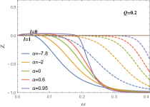
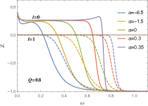
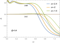
Figure 2: Effects of $\alpha$ on the amplification factor when $q=1$. Solid lines for $l=0$, dashed lines for $l=1$. We take $Q=0.2,0.8$ and $1.4$ as examples to exhibit our results. When $Q=0.2$, the range of $\alpha$ is $(-7.92,0.96)$. When $Q=0.8$, the range of $\alpha$ is $(-6.66,0.36)$. When $Q=1.4$, the range of $\alpha$ is $(-2.61,-1.47)$. We vary $\alpha$ in the reasonable region. The lines with $\alpha=0$ correspond to the RN black hole.

These behaviors can be understood intuitively from the effective potential which were plotted in Fig. 3. Note that the reflected amplitude comes from two sides. The one from the extracted energy near the horizon which should cross over the potential barrier to escape to the infinity, we denote as $\mathcal{R}_{0}$. The one reflected by the effective potential barrier of the incident wave, we denote as $\mathcal{R}_{1}$. We see that as $\alpha$ increases in each panel, the effective potential barrier decreases (the solid lines). The extracted energy from the near horizon can escape to the infinity easier and leads to a larger reflected amplitude $\mathcal{R}_{0}$. Therefore the amplification factor increases as $\alpha$ increases. However, when the frequency $\omega$ is large enough, the superradiance ceases. Now $\mathcal{R}_{0}\to 0$ and $\mathcal{R}_{1}$ dominates. The lower effective potential barrier, the smaller reflected amplitude $\mathcal{R}_{1}$. The total amplification factor should decrease as $\alpha$ increases now. This phenomenon can be seen indeed in the far left panel of Fig. 2.

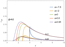
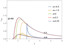
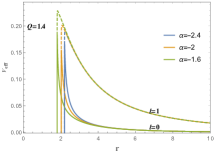
Figure 3: The effective potential corresponding to those with the same parameters in Fig. 2. Solid lines for $l=0$, dashed lines for $l=1$.

Now we turn to the cases of $l=1$(the dashed lines in Fig. 2 and Fig. 3). In each panel of Fig. 2, we see that compared to the cases of $l=0$, the amplification factor is much suppressed in the region (3.9). But the reflected amplitude is nonzero due to the superradiance. It is in fact almost equal to the incident amplitude due to the superradiance. This phenomenon is very different from the neutral cases, where the reflected amplitude is suppressed heavily in the whole frequency region for larger $l$. Beyond the superradiance region (3.9), the amplification factor of $l=1$ becomes larger than that of $l=0$. This can also be understood from the effective potential, as shown in Fig. 3. The effective potential barrier increases with $l$. Beyond the superradiance region, the waves with lower $l$ are more likely to cross over the potential barrier and be absorbed by the black hole and thus leading to smaller amplification factor. The wave with higher $l$ is more likely to be reflected by the higher barrier. Thus the amplification factor is enhanced for larger $l$.

4.2 The effects of $\alpha$ at different $l$ and $Q$ when $q=5$

We take the same parameters as those in the last subsection, except by setting $q=5$, to study the effect of $q$ on the amplification factor. Unlike to $Q$, the parameter $q$ is unlimited in principle. The amplification factors are shown in Fig. 4. In each panel, we see the similar behaviors as those in Fig. 2. But now the amplification factor is much enhanced in the whole frequency region by $q$. Even the higher $l$ modes can have significant amplification factors. The superradiance region $0<\omega<\frac{qQ}{r_{+}}$ is also enlarged by $q$. Interestingly, there appears a peak in the amplification factor before it falls. When $Q=0.2$ and $\alpha=0.95$ (the nearly extremal black hole), this peak rises to nearly 100% above the amplification factor of the lower frequency. When $Q=0.8$, the step-like behavior of the amplification factor becomes more obvious. Note that though the superradiance region is changed by $\alpha$, the amplification factor is almost unchanged with $\alpha$. All the modes satisfying the condition (3.9) are amplified equally.

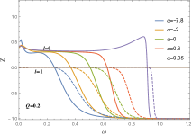
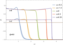
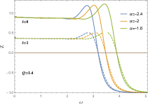
Figure 4: Effects of $\alpha$ on the amplification factor $Z$ when $q=5$. The other parameters are the same as those in Fig. 2. The lines with $\alpha=0$ correspond to the cases of the RN black hole. The small wiggles for small $\omega$ are caused by numerical error.

4.3 The condition for instability

We have shown the superradiance of the 4D charged EGB black hole under the charged scalar perturbation. Since the incident wave can be amplified when its frequency satisfies (3.9), one may suspect that the system is unstable. To clarify this, here we show the condition for the instability.

Multiplying (3.5) by the complex conjugate $\Psi_{0}^{\ast}$ on both sides and integrating it, we get

$$\left.\Psi_{0}^{\ast}\frac{\partial\Psi_{0}}{\partial r_{\ast}}\right|_{-\infty}^{\infty}+\intop_{-\infty}^{\infty}\left(\omega-\frac{qQ}{r}\right)^{2}\left|\Psi_{0}\right|^{2}dr_{\ast}=\intop_{-\infty}^{\infty}V_{\text{eff}}\left|\Psi_{0}\right|^{2}dr_{\ast}+\intop_{-\infty}^{\infty}\left|\frac{\partial\Psi_{0}}{\partial r_{\ast}}\right|^{2}dr_{\ast}.$$ (4.2)

The right hand side is real. Using the boundary condition (3.7) and taking the imaginary part of both sides, we get a relation

$$(a^{2}+b^{2})^{1/4}\cos\left(\frac{1}{2}\arctan\frac{b}{a}\right)+\omega_{R}-\frac{qQ}{r_{+}}+\intop_{-\infty}^{\infty}2\omega_{I}\left(\omega_{R}-\frac{qQ}{r_{+}}\right)\Psi_{0}^{\ast}\Psi_{0}dr_{\ast}=0.$$ (4.3)

Here $\omega=\omega_{R}+i\omega_{I}$ and $a=\omega_{R}^{2}-\omega_{I}^{2}$, $b=2\omega_{R}\omega_{I}$. Since $\arctan\frac{b}{a}\in\left(-\frac{\pi}{2},\frac{\pi}{2}\right)$, the first term is always positive.

The instability implies $\omega_{I}>0$. When $\omega_{I}>0$, there must be $\omega_{R}<\frac{qQ}{r_{+}}$ to keep the above formula hold. But when $\omega_{R}<\frac{qQ}{r_{+}}$, the sign of $\omega_{I}$ can not be determined. This means that the superradiance is the necessary but not sufficient condition for instability. To confirm the instability, one must ensure that the imaginary part of the frequency is positive.

In the following section, we will show numerically that the eigenfrequencies of the system have always negative imaginary part. Therefore, the system is stable, though it has supperradiance. In fact, to trigger the instability, there should be an effective potential well outside the event horizon to trap the reflected wave from the near horizon region. However, it is easy to show that no potential well outside the event horizon and thus no instability of this background under charged scalar perturbations.

5 The stability of the novel 4D charged EGB black hole

We studied the amplification factor by considering the system as a scattering process. To get the eigenfrequencies of the charged scalar perturbation, we should take the system as an eigenvalue problem. The boundary condition now was chosen as

$$\Psi_{0}\to \begin{cases}e^{-i\left(\omega-\frac{qQ}{r_{+}}\right)r_{\ast}}\sim\left(r-r_{+}\right)^{-\frac{i}{2\kappa}\left(\omega-\frac{qQ}{r_{+}}\right)},&r\to r_{+},\\ e^{i\omega r_{\ast}}\sim r^{i\omega r_{+}}e^{i\omega r},&r\to\infty,\end{cases}$$ (5.1)

where we used

$$r_{\ast}\to\begin{cases}\frac{1}{2\kappa}\ln(r-r_{+}),&r\to r_{+}.\\ r+r_{+}\ln(r-r_{+}),&r\to\infty.\end{cases}$$ (5.2)

There is only ingoing waves near the event horizon and outgoing waves at the infinity. The system is dissipative and the frequency of the perturbations will be the composition of quasinormal modes (QNMs). Many numerical methods are developed to solve the quasinormal modes, such as the shooting method, the WKB approximation method, the Horowitz-Hubeny method and the continued fraction method (CFM) [38]. But here we will use the asymptotic iteration method (AIM) [32].

5.1 The asymptotic iteration method

The AIM was used to solve the eigenvalue problem of the homogeneous second order differential equation [39]. Let us introduce a new variable first

$$\xi=1-\frac{r_{+}}{r}.$$ (5.3)

It ranges from 0 to 1 as $r$ runs from the event horizon to the infinity. The radial equation (3.5) becomes

$$0= \frac{f(1-\xi)^{2}}{r_{+}}\left(\frac{\partial^{2}\Psi_{0}}{\partial\xi^{2}}\frac{f(1-\xi)^{2}}{r_{+}}+\frac{\partial\Psi_{0}}{\partial\xi}\frac{(1-\xi)^{2}\partial_{\xi}f-2f(1-\xi)}{r_{+}}\right)$$

$$+\left(\left(\omega-\frac{qQ}{r_{+}}(1-\xi)\right)^{2}-\frac{(1-\xi)^{2}}{r_{+}^{2}}f\left(l(l+1)+(1-\xi)\partial_{\xi}f\right)\right)\Psi_{0}.$$ (5.4)

The solution satisfying the asymptotic behavior (5.1) in terms of $\xi$ has the following form

$$\Psi_{0}= \xi^{-\frac{i}{2\kappa}\left(\omega-\frac{qQ}{r_{+}}\right)}\left(\frac{1}{1-\xi}\right)^{i\omega r_{+}}e^{i\frac{\omega r_{+}}{1-\xi}}\chi(\xi),$$ (5.5)

in which $\chi(\xi)$ is a regular function of $\xi$ in range $(0,1)$. Function $\chi(\xi)$ obeys a homogeneous second order differential equation

$$\frac{\partial^{2}\chi}{\partial\xi^{2}} = \lambda_{0}(\xi)\frac{\partial\chi}{\partial\xi}+s_{0}(\xi)\chi,$$ (5.6)

in which the coefficients

$$-\lambda_{0}(\xi)= -\frac{i}{\kappa\xi}\left(\omega-\frac{qQ}{r_{+}}\right)+\frac{f^{\prime}(\xi)}{f(\xi)}+\frac{2\left(\xi-i\xi r_{+}\omega+2ir_{+}\omega-1\right)}{(\xi-1)^{2}},$$ (5.7)

$$-s_{0}(\xi)= -\frac{1}{(\xi-1)^{4}\xi^{2}}\left(\frac{(\xi-1)^{2}}{2\kappa}\left(\xi^{2}\left(2r_{+}\omega+i\right)-4\xi r_{+}\omega-i\right)\left(\omega-\frac{qQ}{r_{+}}\right)\right)$$ (5.8)

$$-\frac{1}{(\xi-1)^{4}\xi^{2}}\left(\frac{(\xi-1)^{4}}{4\kappa^{2}}\left(\omega-\frac{qQ}{r_{+}}\right){}^{2}+\xi^{2}r_{+}\omega\left(r_{+}\omega(\xi-2)^{2}+i(\xi-1)^{2}\right)\right)$$

$$+i\frac{f^{\prime}(\xi)}{(\xi-1)^{2}\xi f(\xi)}\left(\xi\left(2r_{+}\omega+i\right)-\frac{(\xi-1)^{2}}{2\kappa}\left(\omega-\frac{qQ}{r_{+}}\right)-\xi^{2}\left(r_{+}\omega+i\right)\right)$$

$$-\frac{l(l+1)\xi}{(\xi-1)^{2}\xi f(\xi)}+\frac{1}{(\xi-1)^{4}f(\xi)^{2}}\left((\xi-1)qQ+r_{+}\omega\right){}^{2}.$$

The coefficients $\lambda_{0}(\xi)$ and $s_{0}(\xi)$ are analytical functions in the interval $(0,1)$. Now differentiating (5.6) with respect to $\xi$ iteratively, we get an $(n+2)$-th order differential equation

$$\chi^{(n+2)}=\lambda_{n}(\xi)\chi^{\prime}(\xi)+s_{n}(\xi)\chi(x),$$ (5.9)

where the coefficients can be determined iteratively.

$$\lambda_{n}(\xi)= \lambda^{\prime}_{n-1}(\xi)+s_{n-1}(\xi)+\lambda_{0}(\xi)\lambda_{n-1}(\xi),$$ (5.10)

$$s_{n}(\xi)= s^{\prime}_{n-1}(\xi)+s_{0}(\xi)\lambda_{n-1}(\xi).$$

In asymptotic iteration method, the cutoff of the iteration for large enough $n$ is determined by

$$\frac{s_{n}(\xi)}{\lambda_{n}(\xi)}=\frac{s_{n-1}(\xi)}{\lambda_{n-1}(\xi)}.$$ (5.11)

Then the quasinormal modes $\omega$ can be worked out from this “quantization condition”. To improve the efficiency and accuracy, let us making an expansion around a regular point $\xi=\xi_{0},$

$$\lambda_{n}(\xi)=\sum_{j=0}^{\infty}c_{n}^{j}(\xi-\xi_{0})^{j},s_{n}(\xi)=\sum_{j=0}^{\infty}d_{n}^{j}(\xi-\xi_{0})^{j}.$$ (5.12)

The expansion coefficients $c_{n}^{j}$ and $d_{n}^{j}$ are functions of frequency $\omega$. Substituting the expansions into (5.10), we get iterative relations between these expansion coefficients.

$$c_{n}^{j}= (j+1)c_{n-1}^{j+1}+d_{n-1}^{j}+\sum_{k=0}^{j}c_{0}^{k}c_{n-1}^{j-k},$$ (5.13)

$$d_{n}^{j}= (j+1)d_{n-1}^{i+1}+\sum_{k=0}^{j}d_{0}^{k}c_{n-1}^{j-k}.$$ (5.14)

In terms of the expansion coefficients, the “quantization condition” becomes

$$d_{n}^{0}c_{n-1}^{0}=d_{n-1}^{0}c_{n}^{0}.$$ (5.15)

From this “quantization condition” , we can get the frequency $\omega$ of the perturbation. The efficiency and accuracy of AIM depends on the expansion point $\xi_{0}$. We will ensure the reliability of the results by varying the expansion point $\xi_{0}$ and the iteration times $n$.

5.2 The eigenfrequency of perturbation

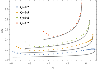
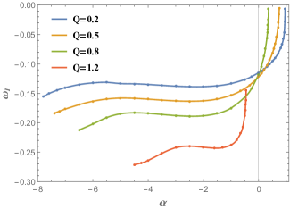
Figure 5: Effects of $\alpha$ on the fundamental quasinormal modes of the charged scalar perturbation when $q=1$. Left panel for real part and right panel for imaginary part of the QNMs. We take $Q=0.2,0.5,0.8$ and $1.2$ as examples to exhibit our results. When $Q=0.2$, the range of $\alpha$ is $(-7.92,0.96)$. When $Q=0.5$, the range of $\alpha$ is $(-7.49,0.75)$. When $Q=0.8$, the range of $\alpha$ is $(-6.66,0.36)$. When $Q=1.2$, the range of $\alpha$ is $(-4.68,-0.44)$. We vary $\alpha$ in the reasonable regions, respectively. The gray lines are corresponding threshold $\frac{qQ}{r_{+}}$ for superadiance since $r_{+}$ depends on $\alpha$.

We plot the fundamental quasinormal modes when $q=1$ in Fig. 5. In the left panel, we see that the real part $\omega_{R}$ of the fundamental QNMs is a concave function of $\alpha$. It also increases monotonically with $Q$. The most interesting point is that all $\omega_{R}$ live above the threshold $\frac{qQ}{r_{+}}$ of superradiance. For positive $\alpha$ or large $Q$, the real part $\omega_{R}$ is very close to the threshold. Therefore there should not be instability of the charged 4D EGB black hole under perturbations. We confirm this in the right panel by noticing that all the imaginary part $\omega_{I}$ of the QNMs are negative. $\omega_{I}$ increases with $\alpha$ at first and then keeps nearly unchanged before it increases with $\alpha$ again. Interestingly, for positive $\alpha,$ $\omega_{I}$ tends to 0 rapidly when the black hole becomes extremal. This implies the extremal 4D charged black hole may have normal modes. For negative $\alpha$, the imaginary part $\omega_{I}$ can not reach 0 and rest on a finite negative value. These phenomenon also exists for higher $l$.

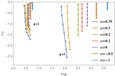
Figure 6: The overtones of the QNMs when $Q=0.8,l=0$. $\alpha$ ranges from -1 to 0.35, where the black hole is nearly extremal. The left hand side is for $q=1$, the right hand side for $q=5$. The case of $\alpha=0$ corresponds to RN black hole.

We show the overtones of the QNMs when $Q=0.8$ and $l=0$ in Fig. 6. The green lines corresponds to the cases of RN black hole. For positive $\alpha,$ we see that the the imaginary part of the overtones increases with $\alpha$. Note that when $\alpha$ makes the black hole nearly extremal, the imaginary part of the fundamental modes tends to zero for both $q=1$ and $q=5$. For negative $\alpha$, the imaginary part of the frequency decreases. When $q$ is small, the real part of the overtones changes very small. While for large $q$, the real part changes significantly.

6 Summary

We studied the parameter region of the novel 4D charged EGB black hole where allows the event horizon. The black hole charge can be larger than the black hole mass due to the existence of negative GB coupling constant $\alpha$.

With the help of appropriate boundary condition, the condition for superradiance was derived. We analyzed the effects of $\alpha$ on the amplification factor of the superradiance in detail. The positive $\alpha$ enhances the superradiance and the negative $\alpha$ suppresses it. Almost all the frequencies satisfying the superradiance condition region are amplified equally. Beyond this region, the reflected wave vanishes rapidly and the amplification factor falls like a step-like function. We analyzed this phenomenon from the viewpoint of effective potential.

To confirm whether the 4D charged EGB black hole has instability, we worked out the QNMs of the system using the asymptotic iteration method. We found that all the real part of the QNMs live beyond the superradiance condition (3.9). The imaginary part of QNMs are negative. Therefore here is no instability. We studied the effects of $\alpha$ on the QNMs in detail. For $\alpha$ that makes black hole extremal, we found that there may be normal modes. Further detailed study on this phenomenon is required.

We further proved the condition for instability of the 4D charged EGB black hole. Though there is superradiance, the system is stable under perturbations due to the absence of an effective potential well outside the event horizon to accumulate the energy and bounce them back to the black hole again. The potential well can be induced by an artificial mirror outside the horizon or by a massive scalar. It has been shown that asymptotically-flat charged black holes are stable against massive charged scalar perturbations [40], but unstable for mirror boundary [41]. Since the potential well also appears in asymptotic dS or AdS spacetime, one can expect the superradiant instability of the 4D charged EGB-(A)dS black holes [42, 43]. In the forthcoming paper, we will study them in detail.

7 Acknowledgments

C.-Y. Zhang is supported by Natural Science Foundation of China under Grant No. 11947067. S.-J. Zhang is supported by National Natural Science Foundation of China (Nos. 11605155 and 11675144). MG and PCL are supported by NSFC Grant No. 11947210. MG is also funded by China National Postdoctoral Innovation Program 2019M660278.

References

- [1] R. Penrose and R. Floyd, “Extraction of rotational energy from a black hole,” Nature 229 (1971), 177-179
-
[2]
Y. B. Zel’ dovich, “Amplification of Cylindrical Electromagnetic Waves Reflected from a Rotating Body,” Soviet Physics-JETP 35, 1085 (1972).
A. A. Starobinskij, “Amplification of waves during reflection from a rotating black hole,” Zhurnal Eksperimentalnoi i Teoreticheskoi Fiziki 64, 48 (1973).
W. H. Press and S. A. Teukolsky, “Floating Orbits, Superradiant Scattering and the Black-hole Bomb,” Nature 238 (1972), 211-212 - [3] J. D. Bekenstein, “Extraction of energy and charge from a black hole,” Phys. Rev. D 7, 949 (1973).
- [4] S. W. Hawking and H. S. Reall, “Charged and rotating AdS black holes and their CFT duals,” Phys. Rev. D 61 (2000) 024014 [hep-th/9908109].
- [5] R. Brito, V. Cardoso and P. Pani, “Superradiance : Energy Extraction, Black-Hole Bombs and Implications for Astrophysics and Particle Physics,” Lect. Notes Phys. 906, pp.1 (2015) [arXiv:1501.06570 [gr-qc]].
- [6] L. Di Menza and J. P. Nicolas, “Superradiance on the Reissner–Nordstrom metric,” Class. Quant. Grav. 32, no. 14, 145013 (2015) [arXiv:1411.3988 [math-ph]].
- [7] M. Richartz and A. Saa, “Challenging the weak cosmic censorship conjecture with charged quantum particles,” Phys. Rev. D 84, 104021 (2011) [arXiv:1109.3364 [gr-qc]].
-
[8]
Y. S. Myung,
“Instability of rotating black hole in a limited form of gravity,”
Phys. Rev. D 84, 024048 (2011)
[arXiv:1104.3180 [gr-qc]].
Y. S. Myung, “Instability of a Kerr black hole in gravity,” Phys. Rev. D 88, no. 10, 104017 (2013) [arXiv:1309.3346 [gr-qc]].
C. Y. Zhang, S. J. Zhang, and B. Wang, “Superradiant instability of Kerr-de Sitter black holes in scalar-tensor theory”, J. High Energy Phys. 08 (2014) 011. arXiv:1405.3811.
C. Y. Zhang, S. J. Zhang, and B. Wang, Charged scalar perturbations around Garfinkle–Horowitz–Strominger black holes, Nucl. Phys. B899, 37 (2015). arXiv:1501.03260.
M. F. Wondrak, P. Nicolini and J. W. Moffat, “Superradiance in Modified Gravity (MOG),” JCAP 1812, 021 (2018) [arXiv:1809.07509 [gr-qc]].
M. Khodadi, A. Talebian and H. Firouzjahi, “Black Hole Superradiance in f(R) Gravities,” arXiv:2002.10496 [gr-qc]. - [9] T. Clifton, P. G. Ferreira, A. Padilla and C. Skordis, “Modified Gravity and Cosmology,” Phys. Rept. 513, 1 (2012) [arXiv:1106.2476 [astro-ph.CO]].
- [10] D. Glavan and C. Lin, Einstein-Gauss-Bonnet gravity in 4-dimensional space-time, Phys. Rev. Lett. 124, no. 8, 081301 (2020), arXiv:1905.03601 [gr-qc].
-
[11]
R. G. Cai, L. M. Cao and N. Ohta,
“Black Holes in Gravity with Conformal Anomaly and Logarithmic Term in Black Hole Entropy,”
JHEP 1004, 082 (2010), arXiv:0911.4379.
Y. Tomozawa, “Quantum corrections to gravity,” arXiv:1107.1424 [gr-qc].
G. Cognola, R. Myrzakulov, L. Sebastiani and S. Zerbini, “Einstein gravity with Gauss-Bonnet entropic corrections,” Phys. Rev. D 88, no. 2, 024006 (2013), arXiv:1304.1878. -
[12]
R. A. Konoplya and A. F. Zinhailo,
“Quasinormal modes, stability and shadows of a black hole in the novel 4D Einstein-Gauss-Bonnet gravity,”
arXiv:2003.01188 [gr-qc].
R. A. Konoplya and A. Zhidenko, “Black holes in the four-dimensional Einstein-Lovelock gravity,” arXiv:2003.07788 [gr-qc].
R. A. Konoplya and A. Zhidenko, “BTZ black holes with higher curvature corrections in the 3D Einstein-Lovelock theory,” arXiv:2003.12171 [gr-qc].
R. A. Konoplya and A. Zhidenko, “(In)stability of black holes in the 4D Einstein-Gauss-Bonnet and Einstein-Lovelock gravities,” arXiv:2003.12492 [gr-qc].
R. A. Konoplya and A. F. Zinhailo, “Grey-body factors and Hawking radiation of black holes in 4D Einstein-Gauss-Bonnet gravity,” arXiv:2004.02248 [gr-qc]. -
[13]
M. Guo and P. C. Li,
“The innermost stable circular orbit and shadow in the novel Einstein-Gauss-Bonnet gravity,”
arXiv:2003.02523 [gr-qc].
C. Y. Zhang, P. C. Li and M. Guo, “Greybody factor and power spectra of the Hawking radiation in the novel Einstein-Gauss-Bonnet de-Sitter gravity,” arXiv:2003.13068. - [14] P. G. S. Fernandes, “Charged Black Holes in AdS Spaces in Einstein Gauss-Bonnet Gravity,” arXiv:2003.05491 [gr-qc].
- [15] A. Casalino, A. Colleaux, M. Rinaldi and S. Vicentini, “Regularized Lovelock gravity,” arXiv:2003.07068 [gr-qc].
-
[16]
S. W. Wei and Y. X. Liu,
“Testing the nature of Gauss-Bonnet gravity by four-dimensional rotating black hole shadow,”
arXiv:2003.07769 [gr-qc].
Y. P. Zhang, S. W. Wei and Y. X. Liu, “Spinning test particle in four-dimensional Einstein-Gauss-Bonnet Black Hole,” arXiv:2003.10960 [gr-qc].
S. W. Wei and Y. X. Liu, “Extended thermodynamics and microstructures of four-dimensional charged Gauss-Bonnet black hole in AdS space,” arXiv:2003.14275 [gr-qc]. -
[17]
R. Kumar and S. G. Ghosh,
“Rotating black holes in the novel Einstein-Gauss-Bonnet gravity,”
arXiv:2003.08927 [gr-qc].
S. G. Ghosh and S. D. Maharaj, “Radiating black holes in the novel 4D Einstein-Gauss-Bonnet gravity,” arXiv:2003.09841 [gr-qc].
S. G. Ghosh and R. Kumar, “Generating black holes in the novel Einstein-Gauss-Bonnet gravity,” arXiv:2003.12291 [gr-qc].
D. V. Singh, S. G. Ghosh and S. D. Maharaj, “Clouds of string in novel Einstein-Gauss-Bonnet black holes,” arXiv:2003.14136 [gr-qc].
A. Kumar and S. G. Ghosh, “Hayward black holes in the novel Einstein-Gauss-Bonnet gravity,” arXiv:2004.01131 [gr-qc].
S. U. Islam, R. Kumar and S. G. Ghosh, “Gravitational lensing by black holes in Einstein-Gauss-Bonnet gravity,” arXiv:2004.01038 [gr-qc].
A. Kumar and R. Kumar, “Bardeen black holes in the novel Einstein-Gauss-Bonnet gravity,” arXiv:2003.13104 [gr-qc]. - [18] K. Hegde, A. N. Kumara, C. L. A. Rizwan, A. K. M. and M. S. Ali, “Thermodynamics, Phase Transition and Joule Thomson Expansion of novel 4-D Gauss Bonnet AdS Black Hole,” arXiv:2003.08778 [gr-qc].
- [19] D. D. Doneva and S. S. Yazadjiev, “Relativistic stars in 4D Einstein-Gauss-Bonnet gravity,” arXiv:2003.10284 [gr-qc].
- [20] H. Lu and Y. Pang, “Horndeski Gravity as Limit of Gauss-Bonnet,” arXiv:2003.11552 [gr-qc].
- [21] D. V. Singh and S. Siwach, “Thermodynamics and P-v criticality of Bardeen-AdS Black Hole in 4-D Einstein-Gauss-Bonnet Gravity,” arXiv:2003.11754 [gr-qc].
- [22] T. Kobayashi, “Effective scalar-tensor description of regularized Lovelock gravity in four dimensions,” arXiv:2003.12771 [gr-qc].
- [23] S. A. Hosseini Mansoori, “Thermodynamic geometry of novel 4-D Gauss Bonnet AdS Black Hole,” arXiv:2003.13382 [gr-qc].
- [24] M. S. Churilova, “Quasinormal modes of the Dirac field in the novel 4D Einstein-Gauss-Bonnet gravity,” arXiv:2004.00513 [gr-qc].
- [25] A. K. Mishra, “Quasinormal modes and Strong Cosmic Censorship in the novel 4D Einstein-Gauss-Bonnet gravity,” arXiv:2004.01243 [gr-qc].
- [26] S. Nojiri and S. D. Odintsov, “Novel cosmological and black hole solutions in Einstein and higher-derivative gravity in two dimensions,” arXiv:2004.01404 [hep-th].
- [27] C. Liu, T. Zhu and Q. Wu, “Thin Accretion Disk around a four-dimensional Einstein-Gauss-Bonnet Black Hole,” arXiv:2004.01662 [gr-qc].
- [28] S. L. Li, P. Wu and H. Yu, “Stability of the Einstein Static Universe in 4D Gauss-Bonnet Gravity,” arXiv:2004.02080 [gr-qc].
- [29] M. Heydari-Fard, M. Heydari-Fard and H. R. Sepangi, “Bending of light in novel 4D Gauss-Bonnet-de Sitter black holes by Rindler-Ishak method,” [arXiv:2004.02140[gr-qc]].
- [30] X. h. Jin, Y.-x. Gao and D. j. Liu “Strong gravitational lensing of a 4D Einstein-Gauss-Bonnet black hole in homogeneous plasma,” [arXiv:2004.02261[gr-qc]].
- [31] W. Y. Ai “A note on the novel 4D Einstein-Gauss-Bonnet gravity,” [arXiv:2004.02858[gr-qc]].
-
[32]
H. T. Cho, A. S. Cornell, J. Doukas, W. Naylor,
Black hole quasinormal modes using the asymptotic iteration method.
Class. Quant. Grav. 2010, 27: 155004, arXiv:0912.2740.
H. T. Cho, A. S. Cornell, J. Doukas, T. R. Huang, W. Naylor, A New Approach to Black Hole Quasinormal Modes: A Review of the Asymptotic Iteration Method. Adv. Math. Phys. 2012, 2012: 281705, arXiv:1111.5024 [gr-qc]. - [33] T. Pappas, P. Kanti, N. Pappas, Hawking Radiation Spectra for Scalar Fields by a Higher-Dimensional Schwarzschild-de-Sitter Black Hole, Phys.Rev. D94 (2016) no.2, 024035, arXiv:1604.08617 [hep-th].
- [34] J. Ahmed and K. Saifullah, “Greybody factor of a scalar field from Reissner–Nordström–de Sitter black hole,” Eur. Phys. J. C 78, no. 4, 316 (2018) [arXiv:1610.06104 [gr-qc]].
-
[35]
C.-Y. Zhang, P.-C. Li, B. Chen, “Greybody factors
for Spherically Symmetric Einstein-Gauss-Bonnet-de Sitter black hole,”
Phys.Rev. D97 (2018) no.4, 044013, arXiv:1712.00620.
P.-C. Li, C.-Y. Zhang, “Hawking radiation for scalar fields by Einstein-Gauss-Bonnet-de Sitter black holes,” Phys.Rev. D99 (2019) no.2, 024030, arXiv:1901.05749 [hep-th]. - [36] J. Grain, A. Barrau and P. Kanti, “Exact results or evaporating black holes in curvature-squared lovelock gravity: Gauss-Bonnet greybody factors,” Phys. Rev. D 72, 104016 (2005) [hep-th/0509128].
- [37] T. Harmark, J. Natario and R. Schiappa, “Greybody Factors for d-Dimensional Black Holes,” Adv. Theor. Math. Phys. 14, no. 3, 727 (2010) [arXiv:0708.0017 [hep-th]].
- [38] R. A. Konoplya, A. Zhidenko, Quasinormal modes of black holes: From astrophysics to string theory, Rev.Mod.Phys. 83 (2011) 793-836, arXiv:1102.4014 [gr-qc].
-
[39]
R. L. H. H. Ciftci and N. Saad. Asymptotic iteration
method for eigenvalue problems, Journal of Physics A, 2003, vol.36,
no. 47: 11807–11816, arXiv:math-ph/0309066.
R. L. H. H. Ciftci and N. Saad. Perturbation theory in a framework of iteration methods, Physics Letters A, 2005, vol. 340, no. 5-6: 388–396, arXiv:math-ph/0504056. -
[40]
S. Hod, Stability of the extremal Reissner-Nordstrom black hole to charged scalar perturbations, Phys.Lett. B713 (2012) 505-508, arXiv:1304.6474[gr-qc].
S. Hod, No-bomb theorem for charged Reissner-Nordstrom black holes, Phys.Lett. B718 (2013) 1489-1492. arXiv:1304.6474 [gr-qc]. - [41] C. A. R. Herdeiro, J. C. Degollado and H. F. Rúnarsson, “Rapid growth of superradiant instabilities for charged black holes in a cavity,” Phys. Rev. D 88, 063003 [arXiv:1305.5513 [gr-qc]]. J. C. Degollado and C. A. R. Herdeiro, “Time evolution of superradiant instabilities for charged black holes in a cavity,” Phys. Rev. D 89, 063005 [arXiv:1312.4579 [gr-qc]]. N. Sanchis-Gual, J. C. Degollado, P. J. Montero, J. A. Font and C. Herdeiro, “Explosion and final state of an unstable Reissner-Nordstrom black hole,” Phys. Rev. Lett 116, 141101 [arXiv:1512.05358 [gr-qc]]. N. Sanchis-Gual, J. C. Degollado, J. A. Font, C. Herdeiro and E. Radu, “Dynamical formation of a hairy black hole in a cavity from the decay of unstable solitons,” Classical and Quantum Gravity, Volume 34, Number 16 [arXiv:1611.02441 [gr-qc]].
- [42] Z. Zhu, S. J. Zhang, C. E. Pellicer, B. Wang and E. Abdalla, “Stability of Reissner-Nordström black hole in de Sitter background under charged scalar perturbation,” Phys. Rev. D 90, no. 4, 044042 (2014) Addendum: [Phys. Rev. D 90, no. 4, 049904 (2014)] [arXiv:1405.4931 [hep-th]].
- [43] R. A. Konoplya and A. Zhidenko, “Charged scalar field instability between the event and cosmological horizons,” Phys. Rev. D 90, no. 6, 064048 (2014) [arXiv:1406.0019 [hep-th]].