RYANSQL: Recursively Applying Sketch-based Slot Fillings
for Complex Text-to-SQL in Cross-Domain Databases

Abstract

Text-to-SQL is the problem of converting a user question into an SQL query, when the question and database are given. In this paper, we present a neural network approach called RYANSQL (Recursively Yielding Annotation Network for SQL) to solve complex Text-to-SQL tasks for cross-domain databases. Statement Position Code (SPC) is defined to transform a nested SQL query into a set of non-nested SELECT statements; a sketch-based slot filling approach is proposed to synthesize each SELECT statement for its corresponding SPC. Additionally, two input manipulation methods are presented to improve generation performance further. RYANSQL achieved 58.2% accuracy on the challenging Spider benchmark, which is a 3.2%p improvement over previous state-of-the-art approaches. At the time of writing, RYANSQL achieves the first position on the Spider leaderboard.

1 Introduction

Text-to-SQL is the task of generating SQL queries when database and natural language user questions are given. Recently proposed neural net architectures achieved more than 80% exact matching accuracy on the well-known Text-to-SQL benchmarks such as ATIS, GeoQuery and WikiSQL (Xu et al., 2017; Yu et al., 2018a; Shi et al., 2018; Dong and Lapata, 2018; Hwang et al., 2019; He et al., 2019). However, those benchmarks have shortcomings of either assuming the same database across the training and test dataset(ATIS, GeoQuery) or assuming the database of a single table and restricting the complexity of SQL query to have a unitary SELECT statement with a single SELECT and WHERE clause (WikiSQL).

Different from those benchmarks, the Spider benchmark proposed by Yu et al. (2018b) contains complex SQL queries with cross-domain databases. Cross-domain means that the databases for the training dataset and test dataset are different; the system should predict with an unseen database as its input during testing. Also, different from another cross-domain benchmark WikiSQL, the SQL queries in Spider benchmark contain nested queries with multiple JOINed tables, and clauses like ORDERBY, GROUPBY, and HAVING. Yu et al. (2018b) showed that the state-of-the-art systems for the previous benchmarks do not perform well on the Spider dataset.

In this paper, we propose a novel network architecture called RYANSQL (Recursively Yielding Annotation Network for SQL) to handle such complex, cross-domain Text-to-SQL problem. The proposed approach generates nested queries by recursively yielding its component SELECT statements. A sketch-based slot filling approach is proposed to predict each SELECT statement. In addition, two simple but effective input manipulation methods are proposed to improve the overall system performance. The proposed system improves the previous state-of-the-art system by 3.2%p in terms of the test set exact matching accuracy, using BERT (Devlin et al., 2019). Our contributions are summarized as follows.

• We propose a detailed sketch for the complex SELECT statements, along with a network architecture to fill the slots.

• Statement Position Code (SPC) is introduced to recursively predict nested queries with sketch-based slot filling algorithm.

• We suggest two simple input manipulation methods to improve performance further. Those methods are easy to apply, and they improve the overall system performance significantly.

2 Related Works

Most recent works on Text-to-SQL task used encoder-decoder model. Those works could be classified into three main categories, based on their decoder outputs. Direct Sequence-to-Sequence approaches (Dong and Lapata, 2016; Zhong et al., 2017) generate SQL query tokens as their decoder outputs; due to the risk of generating grammatically incorrect SQL queries, the Direct Sequence-to-Sequence approaches are rarely used in recent works.

Grammar-based approaches generate a sequence of grammar rules and apply the generated rules sequentially to get the resultant SQL query. Shi et al. (2018) defines a structural representation of an SQL query and a set of parse actions to handle the WikiSQL dataset. Guo et al. (2019) defines SemQL queries, which is an abstraction of SQL query in tree form, along with a set of grammar rules to synthesize SemQL queries; Synthesizing SQL query from a SemQL tree structure is straightforward. Bogin et al. (2019) focused on the DB constraints selection problem during the grammar decoding process; they applied global reasoning between question words and database columns/tables.

Sketch-based slot-filling approaches, firstly proposed by Xu et al. (2017) to handle the WikiSQL dataset, define a sketch with slots for SQL queries, and the decoder classifies values for those slots. Sketch-based approaches Hwang et al. (2019) and He et al. (2019) achieved state-of-the-art performances on the WikiSQL dataset, with the aid of BERT (Devlin et al., 2019). However, sketch-based approach on more complex Spider benchmark (Lee, 2019) showed relatively low performance compared to the grammar-based approaches. There are two major reasons: (1) It is hard to define a sketch for Spider queries since the allowed syntax of the Spider SQL queries is far more complicated than that of the WikiSQL queries. (2) Since the sketch-based approaches fill values for the predefined slots, the approaches have difficulties in predicting the nested queries.

In this paper, a sketch-based slot filling approach is proposed to solve the complex Text-to-SQL problem. A detailed sketch for complex SELECT statements is newly proposed, along with Statement Position Code (SPC) to effectively predict for the nested queries.

3 Task Definition

The Text-to-SQL task considered in this paper is defined as follows: Given a question with $n$ tokens $Q=\{w^{Q}_{1},...,w^{Q}_{n}\}$ and a DB schema with $t$ tables and $f$ foreign key relations $D=\{T_{1},...,T_{t},F_{1},...,F_{f}\}$, find $S$, the SQL translation of $Q$. Each table $T_{i}$ consists of a table name with $t_{i}$ words $\{w^{T_{i}}_{1},...,w^{T_{i}}_{t_{i}}\}$, and a set of columns $\{C_{j},...,C_{k}\}$. Each column $C_{j}$ consists of a column name $\{w^{C_{j}}_{1},...,w^{C_{j}}_{c_{j}}\}$, and a marker to check if the column is a primary key.

For an SQL query $S$ we define a non-nested form of $S$, $N(S)=\{(P_{1},S_{1}),...,(P_{l},S_{l})\}$. In the definition, $P_{i}$ is the $i$-th SPC, and $S_{i}$ is its corresponding SELECT statement. Table 1 shows an example of natural language query $Q$, SQL translation $S$ and its non-nested form $N(S)$.

Q	Find the name of airports which do not
	have any flight in and out.
S	SELECT AirportName FROM Airports
	WHERE AirportCode NOT IN
	(SELECT SourceAirport FROM Flights
	UNION
	SELECT DestAirport FROM Flights)
N(S)	$P_{1}$	[ NONE ]
	$S_{1}$	SELECT AirportName
		FROM Airports
		WHERE AirportCode NOT IN $S_{2}$
	$P_{2}$	[ WHERE ]
	$S_{2}$	SELECT SourceAirport
		FROM Flights UNION $S_{3}$
	$P_{3}$	[ WHERE, UNION ]
	$S_{3}$	SELECT DestAirport FROM Flights

Table 1: Example of a user question $Q$, SQL translation $S$, and its non-nested form $N(S)$.

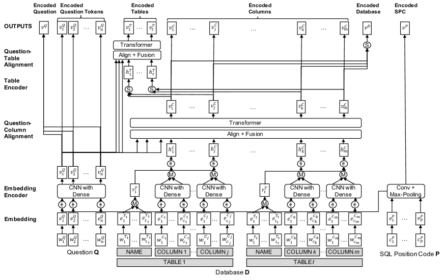
Figure 1: Network architecture of the proposed input encoder. represents vector concatenation, represents max-pooling and represents self-attention.

Each SPC $P$ could be considered as a sequence of $p$ position code elements, $P=[c^{P}_{1},...,c^{P}_{p}]$. The possible set of position code elements is $\{$NONE, UNION, INTERSECT, EXCEPT, WHERE, HAVING, PARALLEL$\}$. NONE represents the outermost statement, while PARALLEL means the parallel elements inside a single clause like the second element of the WHERE clause. Other position code elements represent corresponding SQL clauses.

Since it is straightforward to construct $S$ from $N(S)$, the goal of the proposed system is to construct $N(S)$ for the given $Q$ and $D$. To achieve the goal, the proposed system first sets the initial SPC $P_{1}=[\texttt{NONE}]$, and predicts its corresponding SELECT statement and nested SPCs. The system recursively finds out the corresponding SELECT statements for remaining SPCs, until every SPC has its corresponding SELECT statement.

4 Generating a SELECT Statement

In this section, the method to create the SELECT statement for the given question $Q$, database $D$, and SPC $P$ is described. Section 4.1 describes the input encoder; the sketch-based slot-filling decoder is described in section 4.2.

4.1 Input Encoder

Figure 1 shows the overall network architecture. The input encoder consists of five layers: Embedding layer, Embedding Encoder layer, Question-Column Alignment layer, Table Encoder layer, and Question-Table Alignment layer.

Embedding.

To get the embedding vector for a word $w$ in question, table names or column names, its word embedding and character embedding are concatenated. The word embedding is initialized with $d_{1}=300$-dimensional pre-trained GloVe (Pennington et al., 2014) word vectors, and is fixed during training. For character embedding, each character is represented as a trainable vector of dimension $d_{2}=50$, and we take maximum value of each dimension of component characters to get the fixed-length vector. The two vectors are then concatenated to get the embedding vector $e_{w}\in\mathbb{R}^{d_{1}+d_{2}}$. One layer highway network (Srivastava et al., 2015) is applied on top of this representation. For SPC $P$, each code element $c$ is represented as a trainable vector of dimension $d_{p}=100$.

Embedding Encoder.

One dimensional convolution layer with kernel size 3 is applied on SPC element embedding vectors $\{e^{P}_{1},...,e^{P}_{p}\}$. Max-pooling is applied on the output to get the SPC vector $v^{P}\in\mathbb{R}^{p\times d_{p}}$. $v^{P}$ is then concatenated to each question and column word embedding vector.

CNN with Dense Connection proposed in Yoon et al. (2018) is applied to encode each word of question and columns to capture local information. Parameters are shared across the question and columns. For each column, a max-pooling layer is followed; outputs are concatenated with their table name representations and projected to dimension $d$. Layer outputs are encoded question words $V^{Q}=\{v^{Q}_{1},v^{Q}_{2},...,v^{Q}_{n}\}\in\mathbb{R}^{n\times d}$, and hidden column vectors $H^{C}=\{h^{C}_{1},...,h^{C}_{m}\}\in\mathbb{R}^{m\times d}$.

Question-Column Alignment.

In this layer, the column vectors are modeled with contextual information of the question by attending question tokens with their corresponding columns. Scaled dot-product attention (Vaswani et al., 2017) is used to align question tokens with column vectors:

$$A_{QtoC} =\text{softmax}(\frac{H^{C}\cdot(V^{Q})^{\intercal}}{\sqrt{d}})\cdot V^{Q}$$ (1)

Where each $i$-th row of $A_{QtoC}\in\mathbb{R}^{m\times d}$ is an attended question vector of the $i$-th column.

The heuristic fusion function $fusion(x,y)$, proposed in Hu et al. (2018), is applied to merge $A_{QtoC}$ with $H^{C}$:

$$\tilde{x} =\text{relu}(W_{r}[x;y;x\circ y;x-y])$$

$$g =\sigma(W_{g}[x;y;x\circ y;x-y])$$

$$fusion(x,y) =g\circ\tilde{x}+(1-g)\circ x$$

$$F^{C} =fusion(A_{QtoC},H^{C})$$ (2)

Where $W_{r}$ and $W_{g}$ are trainable variables, $\sigma$ denotes the sigmoid function, $\circ$ denotes element-wise multiplication and $F^{C}\in\mathbb{R}^{m\times d}$ is fused column matrix. A transformer layer (Vaswani et al., 2017) is applied on top of $F^{C}$ to capture contextual column information. Layer outputs are the encoded column vectors $V^{C}=\{v^{C}_{1},...,v^{C}_{m}\}\in\mathbb{R}^{m\times d}$.

Table Encoder.

Column vectors belonging to each table are integrated to get the encoded table vector. For a matrix $M\in\mathbb{R}^{n\times d}$, self-attention function $f_{s}(M)\in\mathbb{R}^{1\times d}$ is defined as follows:

$$f_{s}(M) =\text{softmax}(W_{2}\tanh(W_{1}M^{\intercal}))M$$ (3)

Where $W_{1}\in\mathbb{R}^{d\times d}$, $W_{2}\in\mathbb{R}^{1\times d}$ are trainable parameters. Then, for table $t$ with columns $\{C_{j},...,C_{k}\}$, the hidden table vector $h^{T}_{t}$ is calculated as follows:

$$h^{T}_{t} =f_{s}([v^{C}_{j};...;v^{C}_{k}])$$ (4)

Layer outputs are the hidden table vectors $H^{T}=\{h^{T}_{1},h^{T}_{2},...,h^{T}_{t}\}\in\mathbb{R}^{t\times d}$.

Question-Table Alignment.

In this layer, the same network architecture as the Question-Column alignment layer is used to model the table vectors with contextual information of the question. Layer outputs are the encoded table vectors $V^{T}=\{v^{T}_{1},v^{T}_{2},...,v^{T}_{t}\}\in\mathbb{R}^{t\times d}$.

Output.

Final outputs of the input encoder are: (1) Encoded question words $V^{Q}=\{v^{Q}_{1},...,v^{Q}_{n}\}\in\mathbb{R}^{n\times d}$, (2) Encoded columns $V^{C}=\{v^{C}_{1},...,v^{C}_{m}\}\in\mathbb{R}^{m\times d}$, (3) Encoded tables $V^{T}=\{v^{T}_{1},...,v^{T}_{t}\}\in\mathbb{R}^{t\times d}$, and (4) Encoded SPC $v^{P}\in\mathbb{R}^{d_{p}}$. Additionally, (5) Encoded question $v^{Q}=f_{s}(V^{Q})$ and (6) Encoded DB schema $v^{D}=f_{s}(V^{C})\in\mathbb{R}^{d}$ are calculated for later use.

4.1.1 BERT-based Input Encoder

Inspired by the work of Hwang et al. (2019) and Guo et al. (2019), BERT (Devlin et al., 2019) is considered as another version of input encoder. The input to BERT is constructed by concatenating question words, SPC elements and column words as follows: [CLS], $w^{Q}_{i}$, [SEP], $c^{P}_{j}$, [SEP], $w^{C_{1}}_{k}$, [SEP], …, $w^{C_{m}}_{l}$, [SEP].

Hidden states of the last layer are retrieved to form $V^{Q}$ and $V^{C}$; for $V^{C}$, the state of each column’s last word is taken to represent encoded column vector. Each table vector $v^{T}_{j}$ is calculated as a self-attended vector of its containing columns; $v^{Q}$, $v^{D}$, and $v^{P}$ are calculated as the same.

4.2 Sketch-based Slot-Filling Decoder

CLAUSE	SKETCH
FROM	$(\texttt{\$TBL})^{+}$
SELECT	$DIST ( $AGG ( $DIST1 $AGG1 $COL1 $ARI $DIST2 $AGG2 $COL2 ) ) +
ORDERBY	( ( $DIST1 $AGG1 $COL1 $ARI $DIST2 $AGG2 $COL2 ) $ORD ) ∗
GROUPBY	( $COL )∗
LIMIT	$NUM
WHERE	( $CONJ ( $DIST1 $AGG1 $COL1 $ARI $DIST2 $AGG2 $COL2 )
HAVING	$NOT $COND $VAL1$|$$SEL1 $VAL2$|$$SEL2 )∗
INTERSECT
UNION	$SEL
EXCEPT

Table 2: Proposed sketch for a SELECT statement. $TBL and $COL represent a table and a column, respectively. $AGG is one of {none, max, min, count, sum, avg}, $ARI is one of the arithmetic operators {none, -, +, *, / }, and $COND is one of the conditional operators {between, =, >, <, >=, <=, !=, in, like, is, exists}. $DIST and $NOT are boolean variables representing the existence of keywords DISTINCT and NOT, respectively. $ORD is a binary value for keywords ASC/DESC, and $CONJ is one of conjunctions {AND, OR}. $VAL is the value for WHERE/HAVING condition; $SEL represents the slot for another SELECT statement.

Table 2 shows the proposed sketch for a SELECT statement. The sketch-based slot-filling decoder predicts values for slots of the proposed sketch.

Classifying Base Structure.

By the term base structure of a SELECT statement, we refer to the existence of its component clauses and the number of conditions for each clause. We first combine the encoded vectors $v^{Q}$, $v^{D}$ and $v^{P}$ to get the statement encoding vector $v^{S}$, as follows:

$$hc(x,y) =concat(x,y,|x-y|,x\circ y)$$ (5)

$$v^{S} =W\cdot concat(hc(v^{Q},v^{D}),v^{P})$$ (6)

Where $W\in\mathbb{R}^{d\times(4d+d_{p})}$ is a trainable parameter, and function $hc(x,y)$ is the concatenation function for heuristic matching method proposed in Mou et al. (2016).

Eleven values $b_{g},b_{o},b_{l},b_{w},b_{h},n_{g},n_{o},n_{s},n_{w}$, $n_{h}$ and $c_{\texttt{IUEN}}$ are classified by applying two fully-connected layers on $v^{S}$. Binary values $b_{g},b_{o},b_{l},b_{w},b_{h}$ represent the existence of GROUPBY, ORDERBY, LIMIT, WHERE and HAVING, respectively. Note that FROM and SELECT clauses must exist to form a valid SELECT statement. $n_{g},n_{o},n_{s},n_{w},n_{h}$ represent the number of conditions in GROUPBY, ORDERBY, SELECT, WHERE and HAVING clause, respectively. The maximal number of conditions $N_{g}=3$, $N_{o}=3$, $N_{s}=6$, $N_{w}=4$, and $N_{h}=2$ are defined for GROUPBY, ORDERBY, SELECT, WHERE and HAVING clauses, to solve the problem as $n$-way classification problem. The values of maximal condition numbers are chosen to cover all the training cases.

Finally, $c_{\texttt{IUEN}}$ represents the existence of one of INTERSECT, UNION or EXCEPT, or NONE if no such clause exists. If the value of $c_{\texttt{IUEN}}$ is one of INTERSECT, UNION or EXCEPT, the corresponding SPC is created, and the SELECT statement for that SPC is generated recursively.

FROM clause.

A list of $TBLs should be decided to predict the FROM clause. For each table $i$, $P_{\textbf{fromtbl}}(i|Q,D,P)$, the probability that table $i$ is included in the FROM clause, is calculated:

$$c_{i} =concat(v^{T}_{i},v^{Q},v^{D},v^{P})$$

$$s_{i} =W_{2}\tanh(W_{1}\cdot c_{i})$$ (7)

$$P_{\textbf{fromtbl}}(i|Q,D,P) =\sigma(s)_{i}$$

Where $W_{1}$, $W_{2}$ are trainable variables, $s=[s_{1},...,s_{t}]\in\mathbb{R}^{t}$ and $\sigma$ denotes the sigmoid function. From now on, we omit the notations $Q$, $D$ and $P$ for the sake of simplicity.

Top $n_{t}$ tables with the highest $P_{\textbf{fromtbl}}(i)$ values are chosen. We set an upper bound $N_{t}=6$ on possible number of tables. The formula to get $P_{\textbf{\#tbl}}(n_{t})$ for each possible $n_{t}$ is:

$$v^{T^{\prime}} =\text{softmax}(s)\cdot V^{T}$$ (8)

$$P_{\textbf{\#tbl}}(n_{t}) =\text{softmax}(full_{2}(v^{T^{\prime}}))$$

In the equation, $full_{2}$ means the application of two fully-connected layers, and table score vector $s$ is from equation 7.

SELECT clause.

The decoder first generates $N_{s}$ conditions to predict the SELECT. Since each condition depends on different parts of $Q$, we calculate attended question vector for each condition:

$$A^{Q}_{\textbf{sel}} =W_{3}\tanh(V^{Q}\cdot W_{1}+v^{P}\cdot W_{2})^{\intercal}$$ (9)

$$V^{Q}_{\textbf{sel}} =\text{softmax}(A^{Q}_{\textbf{sel}})\cdot V^{Q}$$

While $W_{1},W_{2}\in\mathbb{R}^{d\times d}$, $W_{3}\in\mathbb{R}^{N_{s}\times d}$ are trainable parameters, and $V_{\textbf{sel}}^{Q}\in\mathbb{R}^{N_{s}\times d}$ is the matrix of attended question vectors for $N_{s}$ conditions. $v^{P}$ is tiled to match the row of $V^{Q}$.

For $m$ columns and $N_{s}$ conditions, $P_{\textbf{sel\_col1}}\in\mathbb{R}^{N_{s}\times m}$, the probability matrix for each column to fill the slot $COL₁ of each condition, is calculated as follows:

$$A^{C}_{\textbf{sel}}[i] =W_{6}\tanh(V^{Q}_{\textbf{sel}}[i]\cdot W_{4}+V^{C}\cdot W_{5})^{\intercal}$$

$$P_{\textbf{sel\_col1}}[i] =\text{softmax}(A^{C}_{\textbf{sel}}[i])$$ (10)

Where $W_{4},W_{5}\in\mathbb{R}^{d\times d}$ and $W_{6}\in\mathbb{R}^{1\times d}$ are trainable parameters. The notation $M[i]$ is used to represent the $i$-th row of matrix $M$.

The attended question vectors are then updated with selected column information to get the updated question vector $U^{Q}_{\textbf{sel\_col1}}\in\mathbb{R}^{N_{s}\times d}$:

$$U^{C}_{\textbf{sel\_col1}}[i] =P_{\textbf{sel\_col1}}[i]\cdot V^{C}$$ (11)

$$U^{Q}_{\textbf{sel\_col1}}[i] =W_{7}\cdot hc(V^{Q}_{\textbf{sel}}[i],U^{C}_{\textbf{sel\_col1}}[i])$$

Where $W_{7}$ is a trainable variable, and $hc(x,y)$ is defined in equation 5. The probabilities for $DIST₁, $AGG₁, $ARI and $AGG are calculated by applying a fully connected layer on $U^{Q}_{\textbf{sel\_col1}}[i]$.

Equation 10 is reused to calculate $P_{\textbf{sel\_col2}}$, with $V^{Q}_{\textbf{sel}}[i]$ replaced by $U^{Q}_{\textbf{sel\_col1}}[i]$; then $U^{Q}_{\textbf{sel\_col2}}$ is retrieved in the same way as equation 11, and the probabilities of $DIST₂ and $AGG₂ are calculated in the same way as $DIST₁ and $AGG₁. Finally, the $DIST slot, DISTINCT marker for overall SELECT clause, is calculated by applying a fully-connected layer on $v^{S}$.

Once all the slots are filled for $N_{s}$ conditions, the decoder retrieves the first $n_{s}$ conditions to predict the SELECT clause. That is possible since the CNN with Dense Connection used for question encoding (Yoon et al., 2018) captures relative position information. In combine with the SQL consistency protocol of the Spider benchmark (Yu et al., 2018b), we expect the conditions are ordered in the same way as they are presented in $Q$. For the datasets without such consistency protocol, the proposed slot filling method could easily be changed to an LSTM-based model, as shown in Xu et al. (2017).

ORDERBY clause.

The same network structure as a SELECT clause is applied. The only difference is the prediction for $ORD slot; this could be done by applying a fully connected layer on $U^{Q}_{\textbf{ob\_col1}}$, which is the correspondence of $U^{Q}_{\textbf{sel\_col1}}$.

GROUPBY clause.

The same network structure as a SELECT clause is applied. For the GROUPBY case, retrieving only the values of $P_{\textbf{gb\_col1}}$ is enough to fill the necessary slots.

LIMIT clause.

Questions do not contain the $NUM slot value for LIMIT clauses explicitly in many cases, if the questions are for the top-1 result (Example: “Show the name and the release year of the song by the youngest singer”). Thus, the LIMIT decoder first determines if the given $Q$ requests for the top-1 result. If so, the decoder sets the $NUM value to 1; otherwise, it tries to find the specific token for $NUM among the tokens of $Q$ using pointer network (Vinyals et al., 2015). LIMIT top-1 probability $P_{\textbf{limit\_top1}}$ is retrieved by applying a fully-connected layer on $v^{S}$. $P^{Q}_{\textbf{limit\_num}}[i]$, the probability of $i$-th question token for $NUM slot value, is calculated as:

$$A^{Q}_{\textbf{limit\_num}} =W_{3}\tanh(V^{Q}\cdot W_{1}+v^{P}\cdot W_{2})^{\intercal}$$

$$P^{Q}_{\textbf{limit\_num}}[i] =\text{softmax}(A^{Q}_{\textbf{limit\_num}})_{i}$$ (12)

$W_{1}$, $W_{2}\in\mathbb{R}^{d\times d}$, $W_{3}\in\mathbb{R}^{1\times d}$ are trainable parameters.

WHERE clause.

The same network structure as a SELECT clause is applied to get the attended question vectors $V^{Q}_{\textbf{wh}}\in\mathbb{R}^{N_{w}\times d}$, and probabilities for $COL₁, $COL₂, $DIST₁, $DIST₂, $AGG₁, $AGG₂ and $ARI. Besides, a fully-connected layer is applied on $U^{Q}_{\textbf{wh\_col1}}$ to get the probabilities for $CONJ, $NOT and $COND.

A fully-connected layer is applied on $U^{Q}_{\textbf{wh\_col1}}$ and $U^{Q}_{\textbf{wh\_col2}}$ to determine if the condition value for each column is another nested SELECT statement or not. If the value is determined as a nested SELECT statement, the corresponding SPC is generated, and the SELECT statement for the SPC is predicted recursively. If not, the pointer network is used to get the start and end position of the value span from question tokens.

HAVING clause.

The same network structure as a WHERE clause is applied.

5 Two Input Manipulation Methods

Q: What are the papers of Liwen Xiong in 2015?

SQL:

SELECT DISTINCT t3.paperid

FROM writes AS t2

JOIN author AS t1 ON t2.authorid = t1.authorid

JOIN paper AS t3 ON t2.paperid = t3.paperid

WHERE t1.authorname = ”Liwen Xiong”

AND t3.year = 2015;

Table 3: SQL statement with link table. Table writes is not explicitly mentioned in $Q$, but it is used in the JOIN statement to link between tables author and paper.

In this section, we introduce two input manipulation methods to improve the performance of our proposed system further.

5.1 JOIN Table Filtering

In a FROM clause, some tables may be used only to make “link” between other tables; Table 3 shows such an example. Those “link” tables are necessary to create the proper SELECT statement, but they work as noise for Question-Table alignment since they do not have the corresponding tokens in $Q$. Thus, we discard those tables from FROM clauses during training; while inferencing, the link tables are easily recovered using foreign key relations.

5.2 Supplemented Column Names

Table	Column	SCN
tv channel	id	tv channel id
	series name	tv channel series name
tv series	id	tv series id
cartoon	id	cartoon id

Table 4: Examples of supplemented column names. SCN represents Supplemented Column Name.

We supplement the column names with its table names to distinguish between columns with the same name but belonging to different tables and representing different entities. Table names are concatenated in front of their belonging column names to form SCNs, but if the stemmed form of a table name is wholly included in a stemmed form of the column name, the table name is not concatenated. Table 4 shows SCN examples; the three columns with the same name id are distinguished using their SCNs.

6 Experiment

6.1 Experiment Setup

Dataset.

Spider dataset (Yu et al., 2018b) is used to evaluate our proposed system. We use the same data split as Yu et al. (2018b); 206 databases are split into 146 train, 20 dev, and 40 test. All questions for the same database are in the same split; there are 8659 questions for train, 1034 for dev, and 2147 for test. The test set of Spider is not publicly available, so for testing our models are submitted to the data owner. For evaluation, we used exact matching accuracy, with the same definition as defined in Yu et al. (2018b).

Implementation.

The proposed system is implemented with Tensorflow (Abadi et al., 2015). Layernorm (Ba et al., 2016) and dropout (Srivastava et al., 2014) are applied between layers, with a dropout rate of 0.1. Exponential decay with decay rate 0.8 is applied for every 3 epochs. On each epoch, the trained classifier is evaluated against the validation dataset, and the training stops when the exact match score for the validation dataset is not improved for 20 consequent training epochs. Minibatch size is set to 16; learning rate is set to $4e^{-4}$. Loss is defined as the sum of all classification losses from the slot-filling decoder.

For BERT-based input encoding, we downloaded the publicly available pre-trained model of BERT, BERT-Large, Uncased (Whole Word Masking), and fine-tuned the model during training. The learning rate is set to $1e^{-5}$, and minibatch size is set to 4.

6.2 Experimental Results

Table 5 shows the comparisons of our system with several state-of-the-art systems; Evaluation scores for dev and test datasets are retrieved from the Spider leaderboard. The performance of the proposed system is compared with grammar-based systems GrammarSQL (Lin et al., 2019), Global-GNN (Bogin et al., 2019) and IRNet (Guo et al., 2019). Also, we compared the system performance with RCSQL (Lee, 2019), which so far showed the best performance on the Spider dataset using a sketch-based slot-filling approach.

System	Dev	Test
RCSQL	28.5%	24.3%
GrammarSQL	34.8%	33.8%
IRNet	53.2%	46.7%
Global-GNN	52.7%	47.4%
IRNet v2(BERT)	63.9%	55.0%
Ours
RYANSQL	43.4%	-
RYANSQL(BERT)	66.6%	58.2%

Table 5: Comparison results with other state-of-the-art systems

As can be observed from the table, the proposed system RYANSQL improves the previous slot filling based system RCSQL by a large margin of 15%p on the development dataset. With the use of BERT, our system outperforms the current state-of-the-art by 3.2%p on the hidden test dataset, in terms of exact matching accuracy.

Ablation studies are conducted to further figure out the effect of SPC and the two input manipulation methods. Since the test dataset is not publicly available, we use the development dataset to run the tests. The results are presented in Table 6. In addition, the ablation study results of RYANSQL(BERT) for each hardness level is presented in Table 7. The definitions of hardness levels are the same as the definitions in Yu et al. (2018b). In the tables, Proposed means our proposed system, while -SPC means the one without Statement Position Code, -JTF means the one without JOIN Table Filtering, and -SCN means the one without Supplemented Column Names.

Approach	RYANSQL	RYANSQL
		(BERT)
Proposed	43.4%	66.6%
- SPC	38.1%	57.3%
- JTF	41.4%	63.9%
- SCN	37.7%	56.1%

Table 6: Ablation study results of RYANSQL and RYANSQL(BERT).

Approach	Easy	Med-	Hard	Extra
		ium		Hard
Proposed	86.0%	70.5%	54.6%	40.6%
-SPC	85.6%	66.6%	27.0%	22.4%
-JTF	86.8%	66.1%	46.6%	42.4%
-SCN	76.4%	58.2%	46.6%	30.6%

Table 7: Ablation study results of RYANSQL(BERT) for each hardness level.

As can be observed from the tables, the use of SPC significantly improves the system performance, especially for Hard and Extra Hard queries. The result suggests that by introducing the SPC the proposed system could effectively handle the nested queries. The JTF feature showed some improvements over Medium and Hard queries, meaning that the JTF feature is effective for handling the statements with multiple tables and clauses.

Finally, the SCN feature showed the most significant performance improvement among the three proposed features. When the SCN feature is used, the system performances of all hardness levels are improved significantly. The evaluation result suggests that our proposed input encoder network architectures do not integrate the table names efficiently during the encoding process. But the evaluation result also shows that the proposed system could successfully integrate the table names into encoding vectors by simply applying the proposed SCN feature, instead of modifying the network architectures.

6.3 Error Analysis

We analyzed 345 failed examples of the RYANSQL(BERT) system on the development set. 195 of those examples are analyzed to figure out the main reasons for failure.

The most common cause of failure is column selection failure; 68 out of 195 cases (34.9%) suffered from the error. In many of those cases, the correct column name is not mentioned in a question; for example, for the question “What is the airport name for airport ‘AKO’?”, the decoder chooses column AirportName instead of AirportCode as its WHERE clause condition column. As mentioned in Yavuz et al. (2018), cell value examples for each column will be helpful to solve this problem.

The second frequent error is table number classification error; 49 out of 195 cases (25.2%) belong to the category. The decoder occasionally chooses too many tables for the FROM clause, resulting unnecessary table JOINs. Similarly, 22 out of 195 cases (11.3%) were due to condition number classification error. Those errors could be resolved by observing and updating the extracted slot values as a whole; our future work will focus on this problem.

The remaining 150 errors were either hard to be classified into one category, and some of them were due to different representations of the same meaning, for example: “SELECT max(age) FROM Dogs” vs. “SELECT age FROM Dogs ORDER BY age DESC LIMIT 1”.

7 Conclusion

In this paper, we proposed a sketch-based slot filling algorithm for complex, cross-domain Text-to-SQL problem. A detailed sketch for complex SELECT statement prediction is proposed, along with the Statement Position Code to handle nested queries. Also, two input manipulation methods are proposed to enhance the overall system performance further. Our proposed system achieved the state-of-the-art performance on the challenging Spider benchmark dataset.

The error analysis suggests that we should update slot values based on other slots’ prediction results. Our future work will focus on this slot value updating problem.

References

- Abadi et al. (2015) Martín Abadi, Ashish Agarwal, Paul Barham, Eugene Brevdo, Zhifeng Chen, Craig Citro, Greg S. Corrado, Andy Davis, Jeffrey Dean, Matthieu Devin, Sanjay Ghemawat, Ian Goodfellow, Andrew Harp, Geoffrey Irving, Michael Isard, Yangqing Jia, Rafal Jozefowicz, Lukasz Kaiser, Manjunath Kudlur, Josh Levenberg, Dandelion Mané, Rajat Monga, Sherry Moore, Derek Murray, Chris Olah, Mike Schuster, Jonathon Shlens, Benoit Steiner, Ilya Sutskever, Kunal Talwar, Paul Tucker, Vincent Vanhoucke, Vijay Vasudevan, Fernanda Viégas, Oriol Vinyals, Pete Warden, Martin Wattenberg, Martin Wicke, Yuan Yu, and Xiaoqiang Zheng. 2015. TensorFlow: Large-scale machine learning on heterogeneous systems. Software available from tensorflow.org.
- Ba et al. (2016) Jimmy Lei Ba, Jamie Ryan Kiros, and Geoffrey E. Hinton. 2016. Layer normalization. Computing Research Repository, arXiv:1607.06450.
- Bogin et al. (2019) Ben Bogin, Matt Gardner, and Jonathan Berant. 2019. Global reasoning over database structures for text-to-sql parsing. In Proceedings of the 2019 Conference on Empirical Methods in Natural Language Processing and the 9th International Joint Conference on Natural Language Processing (EMNLP-IJCNLP), pages 3650–3655.
- Devlin et al. (2019) Jacob Devlin, Ming-Wei Chang, Kenton Lee, and Kristina Toutanova. 2019. Bert: Pre-training of deep bidirectional transformers for language understanding. In Proceedings of the 2019 Conference of the North American Chapter of the Association for Computational Linguistics: Human Language Technologies, volume 1, pages 4171–4186.
- Dong and Lapata (2016) Li Dong and Mirella Lapata. 2016. Language to logical form with neural attention. In Proceedings of the 54th Annual Meeting of the Association for Computational Linguistics, pages 33–43.
- Dong and Lapata (2018) Li Dong and Mirella Lapata. 2018. Coarse-to-fine decoding for neural semantic parsing. In Proceedings of the 56th Annual Meeting of the Association for Computational Linguistics, pages 731–742.
- Guo et al. (2019) Jiaqi Guo, Zecheng Zhan, Yan Gao, Yan Xiao, Jian-Guang Lou, Ting Liu, and Dongmei Zhang. 2019. Towards complex text-to-sql in cross-domain database with intermediate representation. Computing Research Repository, arXiv:1905.082057.
- He et al. (2019) Pengcheng He, Yi Mao, Kaushik Chakrabarti, and Weizhu Chen. 2019. X-sql: reinforce schema representation with context. Computing Research Repository, arXiv:1908.08113.
- Hu et al. (2018) Minghao Hu, Yuxing Peng, Zhen Huang, Xipeng Qiu, Furu Wei, and Ming Zhou. 2018. Reinforced mnemonic reader for machine reading comprehension. In Proceedings of the 27th International Joint Conference on Artificial Intelligence, pages 4099–4106.
- Hwang et al. (2019) Wonseok Hwang, Jinyeong Yim, Seunghyun Park, and Minjoon Seo. 2019. A comprehensive exploration on wikisql with table-aware word contextualization. Computing Research Repository, arXiv:1902.01069.
- Lee (2019) Dongjun Lee. 2019. Clause-wise and recursive decoding for complex and cross-domain text-to-sql generation. In Proceedings of the 2019 Conference on Empirical Methods in Natural Language Processing and the 9th International Joint Conference on Natural Language Processing (EMNLP-IJCNLP), pages 6047–6053.
- Lin et al. (2019) Kevin Lin, Ben Bogin, Mark Neumann, Jonathan Berant, and Matt Gardner. 2019. Grammar-based neural text-to-sql generation. Computing Research Repository, arXiv:1905.13326.
- Mou et al. (2016) Lili Mou, Rui Men, Ge Li, Yan Xu, Lu Zhang, Rui Yan, and Zhi Jin. 2016. Natural language inference by tree-based convolution and heuristic matching. In Proceedings of the 54th Annual Meeting of the Association for Computational Linguistics, pages 130–136.
- Pennington et al. (2014) Jeffrey Pennington, Richard Socher, and Christopher D. Manning. 2014. Glove: Global vectors for word representation. In Empirical Methods in Natural Language Processing (EMNLP), pages 1532–1543.
- Shi et al. (2018) Tianze Shi, Kedar Tatwawadi, Kaushik Chakrabarti, Yi Mao, Oleksandr Polozov, and Weizhu Chen. 2018. Incsql: Training incremental text-to-sql parsers with non-deterministic oracles. Computing Research Repository, arXiv:1809.05054.
- Srivastava et al. (2014) Nitish Srivastava, Geoffrey Hinton, Alex Krizhevsky, Ilya Sutskever, and Ruslan Salakhutdinov. 2014. Dropout: a simple way to prevent neural networks from overfitting. The Journal of Machine Learning Research, 15(1):1929–1958.
- Srivastava et al. (2015) Rupesh K. Srivastava, Klaus Greff, and Jürgen Schmidhuber. 2015. Training very deep networks. Advances in neural information processing systems., pages 2377–2385.
- Vaswani et al. (2017) Ashish Vaswani, Noam Shazeer, Niki Parmar, Jakob Uszkoreit, Llion Jones, Aidan N. Gomez, Łukasz Kaiser, and Illia Polosukhin. 2017. Attention is all you need. Advances in neural information processing systems., 30:5998–6008.
- Vinyals et al. (2015) Oriol Vinyals, Meire Fortunato, and Navdeep Jaitly. 2015. Pointer networks. Advances in Neural Information Processing Systems, pages 2692–2700.
- Xu et al. (2017) Xiaojun Xu, Chang Liu, and Dawn Song. 2017. Sqlnet: Generating structured queries from natural language without reinforcement learning. Computing Research Repository, arXiv:1711.04436.
- Yavuz et al. (2018) Semih Yavuz, Izzeddin Gur, Yu Su, and Xifeng Yan. 2018. What it takes to achieve 100% condition accuracy on wikisql. Proceedings of the 2018 Conference on Empirical Methods in Natural Language Processing, pages 1702–1711.
- Yoon et al. (2018) Deunsol Yoon, Dongbok Lee, and Sangkeun Lee. 2018. Dynamic self-attention : Computing attention over words dynamically for sentence embedding. Computing Research Repository, arXiv:1808.073837.
- Yu et al. (2018a) Tao Yu, Zifan Li, Zilin Zhang, Rui Zhang, and Dragomir Radev. 2018a. Typesql: Knowledge-based type-aware neural text-to-sql generation. In Proceedings of the 2018 Conference of the North American Chapter of the Association for Computational Linguistics: Human Language Technologies, pages 588–594.
- Yu et al. (2018b) Tao Yu, Rui Zhang, Kai Yang, Michihiro Yasunaga, Dongxu Wang, Zifan Li, James Ma, Irene Li, Qingning Yao, Shanelle Roman, Zilin Zhang, and Dragomir Radev. 2018b. Spider: A large-scale human-labeled dataset for complex and cross-domain semantic parsing and text-to-sql task. In Proceedings of the 2018 Conference on Empirical Methods in Natural Language Processing, pages 3911–3921.
- Zhong et al. (2017) Victor Zhong, Caiming Xiong, and Richard Socher. 2017. Seq2sql: Generating structured queries from natural language using reinforcement learning. Computing Research Repository, arXiv:1709.00103.